Habit persistence and asset pricing:Evidence from Denmark

Tom Engsted∗ Stig V. Møller† Van Minh Tuong‡

December 2005. Revised September 2006.§

Abstract

We use an iterated GMM approach to estimate and test the con-sumption based habit persistence model of Campbell and Cochrane(1999) on quarterly Danish stock and bond returns over the pe-riod 1985-2001. For comparative purposes we also estimate andtest the standard time-separable model based on power utility.In addition, we compare the pricing errors of the different modelsusing Hansen and Jagannathan’s (1997) specification error mea-sure. The empirical results, which are quite robust across differ-ent asset combinations and instrument sets, show that, i) neitherthe Campbell-Cochrane model nor the power utility model arestatistically rejected by Hansen’s J -test; ii) pricing errors are ofthe same magnitude for both models; iii) the risk-free rate ispositive in the power utility model and mostly negative in theCampbell-Cochrane model; iv) in the Campbell-Cochrane modelrisk-aversion does not move countercyclically. These results sug-gest that - in contrast to what characterizes the US -, for Denmarkthe Campbell-Cochrane model does not perform better than thesimple power utility model in explaining asset returns.

Keywords: Campbell and Cochrane model, GMM, Specificationerror.

JEL codes: C32, G12

∗Aarhus School of Business, Fuglesangs allé 4, DK-8210 Aarhus V., tom@asb.dk.†Aarhus School of Business, Fuglesangs allé 4, DK-8210 Aarhus V., svm@asb.dk.‡TDC, Nørregade 21, S 226, 0900 København C., mtu@tdc.dk.§Comments and suggestions from participants at the Summer Econometrics Work-

shop at the University of Aarhus, August 2006, are gratefully acknowledged.

1

1 Introduction

Since Mehra and Prescott’s (1985) seminal study, explaining the ob-served high equity premium within the consumption based asset pricingframework has occupied a large number of researchers in finance andmacroeconomics. Despite an intense research effort, still no consensushas emerged as to why stocks have given such a high average returncompared to bonds. At first sight the natural response to the equitypremium puzzle is to dismiss the consumption based framework alto-gether. However, as emphasized by Cochrane (2005), within the rationalequilibrium paradigm of finance, there is really no alternative to the con-sumption based model, since other models are not alternatives to - butspecial cases of - the consumption based model. Thus, despite its poorempirical performance, the consumption based framework continues todominate studies of the equity premium on the aggregate stock market.In a recent paper Chen and Ludvigson (2006) argue that within the

equilibrium consumption based framework, habit formation models arethe most promising and successful in describing aggregate stock marketbehaviour. The most prominent habit model is the one developed byCampbell and Cochrane (1999). In this model people slowly develophabits for a high or low consumption level, such that risk-aversion be-comes time-varying and countercyclical. The model is able to explainthe high US equity premium and a number of other stylized facts for theUS stock market. A special feature of the model is that the average riskaversion over time is quite high, but the risk-free rate is low and stable.Thus, the model solves the equity premium puzzle by high risk aversion,but without facing a risk-free rate puzzle.Campbell and Cochrane (1999) themselves, and most subsequent ap-

plications of their model, do not estimate and test the model economet-rically. Instead they calibrate the model parameters to match the his-torical risk-free rate and Sharpe ratio, and then simulate a chosen set ofmoments which are informally compared to those based on actual his-torical data. Only a few papers engage in formal econometric estimationand testing of the model. Tallarini and Zhang (2005) use an EfficientMethod of Moments technique to estimate and test the model on USdata. They statistically reject the model and find that it has stronglycounterfactual implications for the risk-free interest rate, although theyalso find that the model performs well in other dimensions. Fillat andGarduno (2005) and Garcia et al. (2005) use an iterated GeneralizedMethod of Moments approach to estimate and test the model on USdata. Fillat and Garduno strongly reject the model by Hansen’s (1982)J -test. On the other hand Garcia et al. do not reject the model atconventional significance levels. However, Garcia et al. face the problem

2

that their iterated GMM approach does not lead to convergence withpositive values of the risk-aversion parameter.To our knowledge, there have been no formal econometric studies of

the Campbell-Cochrane model on data from other countries than theUS. Our paper is a first attempt to fill this gap. We examine theCampbell-Cochrane model’s ability to explain Danish stock and bondreturns. Denmark is interesting because historically over a long periodof time the average return on Danish stocks has not been nearly as highas in the US and most other countries, and at the same time the returnon Danish bonds has been somewhat higher than in other countries, seee.g. Engsted and Tanggaard (1999), Engsted (2002), and Dimson et al.(2002). Thus, the Danish equity premium is not nearly as high as inmost other countries, and might not even be regarded a puzzle.On quarterly Danish data for the period 1985-2001 we estimate and

test both the standard model based on power utility and the Campbell-Cochrane model based on habit formation. We basically follow the it-erated GMM approach set out in Garcia et al. (2005). However, incontrast to Garcia et al., - who use Hansen’s (1982) statistically optimalweighting matrix in the GMM iterations -, we follow Cochrane (2005)’ssuggestion and use the identity matrix as weighting matrix. Therebywe attach equal weight to each of the assets in the application. The useof the identity matrix has the further advantage that in our applicationit leads to convergence with positive values of the risk-aversion para-meter, in contrast to the case where we use Hansen’s weighting matrix(Garcia et al. also face convergence problems, which might be due totheir exclusive use of the Hansen weighting matrix). We also computeHansen and Jagannathan’s (1997) specification error measure based onthe second moment matrix of returns as weighting matrix. This measurehas an intuitively appealing percentage pricing error interpretation, andit allows for direct comparison of the magnitude of pricing errors acrossmodels.Our main findings are as follows. First, neither the Campbell-Cochrane

model nor the power utility model are statistically rejected by Hansen’sJ -test. Second, pricing errors are of the same magnitude for both mod-els. Third, the quarterly real risk-free rate is estimated to be positiveand around 2% in the power utility model, while it is mostly nega-tive (and around -1%) in the Campbell-Cochrane model. Finally, inthe Campbell-Cochrane model risk-aversion does not move countercycli-cally. These results are quite robust across different asset combinationsand instrument sets, and suggest that - in contrast to what characterizesthe US -, for Denmark the Campbell-Cochrane model does not performbetter than the simple power utility model in explaining asset returns.

3

The rest of the paper is organized as follows. The next section brieflypresents the power utility and habit persistence models. Section 3 ex-plains the iterated GMM approach used to estimate the models. Section4 presents the empirical results based on Danish data. Finally, section5 offers some concluding remarks.

2 The consumption based models

In this section we start by describing the standard power utility versionof the consumption based model. Since this version of the model is well-known and familiar to most readers, the description will be very brief.Then we give a more detailed description of the Campbell-Cochranehabit based model.

2.1 The power utility modelStandard asset pricing theory implies that the price of an asset at timet, Pt, is determined by the expected future asset payoff, Yt+1, multipliedby the stochastic discount factor, Mt+1: Pt = Et(Mt+1Yt+1). The payoffis given as prices plus dividends, Yt+1 = Pt+1 +Dt+1, and the stochas-tic discount factor depends on the underlying asset pricing model. Inconsumption based models Mt+1 is the intertemporal marginal rate ofsubstitution in consumption. With power utility (constant relative risk

aversion), U(Ct) =C1−γt −11−γ , where γ ≥ 0 is the degree of relative risk

aversion, the stochastic discount factor becomes Mt+1 = δ³Ct+1Ct

´−γ,

where δ = (1+ tp)−1 and tp is the rate of time-preference. Defining gross

return as Rt+1 =Pt+1+Dt+1

Pt, the asset pricing relationship can be stated

as:

0 = Et

"δ

µCt+1

Ct

¶−γRt+1 − 1

#. (1)

Equation (1) captures the basic idea that risk-adjusted equilibriumreturns are unpredictable. In the consumption based model, risk-adjustmenttakes place by multiplying the raw return with the intertemporal mar-ginal rate of substitution in consumption. Risk-averse consumers want tosmooth consumption over time, and for that purpose they use (dis)invest-ments in the asset, thereby making a direct connection between con-sumption growth and the asset return. The correlation between con-sumption growth and returns then becomes crucial for the equilibriumexpected return. From (1) expected returns are given as:

4

Et [Rt+1] =

1−Covt∙Rt+1, δ

³Ct+1Ct

´−γ¸Et

∙³Ct+1Ct

´−γ¸ (2)

The higher the correlation between consumption growth and returns (thelower the correlation between the stochastic discount factor and returns),the higher will be expected equilibrium return (ceteris paribus), becausethe higher the correlation, the less able the asset will be in helpingto smooth consumption over time, which means that the asset will beconsidered riskier and thereby demand a higher return.Equation (1) lends itself directly to empirical estimation and testing

within the GMM framework, c.f. section 3. Empirically the consumptionbased power utility model has run into trouble because consumptiongrowth and stock returns are not sufficiently positively correlated toexplain the historically observed high return on common stocks, unlessthe degree of risk aversion γ is extremely high. The basic problem is thatunless γ is very high, the variability of the intertemporal marginal rateof substitution cannot match the variability of stock returns. Perhapspeople are highly risk-averse, but then the power utility model facesanother problem, namely that with a high γ, the risk-free rate implied bythe model becomes implausibly high. For the risk-free rate the covariancewith the stochastic discount factor is zero, thus from (2):

Rf,t+1 =1

Et

∙³Ct+1Ct

´−γ¸ (3)

Thus, within the standard power utility framework, the equitypremium puzzle cannot be solved without running into a risk-free ratepuzzle. This has led to the development of alternative utility models witha higher volatility of the stochastic discount factor, and with plausibleimplications for the risk-free rate. The habit persistence model describedin the next subsection is one such model.

2.2 The Campbell-Cochrane modelHabit formation models differ from the standard power utility model byletting the utility function be time-nonseparable in the sense that theutility at time t depends not only on consumption at time t, but also onprevious periods consumption. The basic idea is that people get used toa certain standard of living and thereby the utility of some consumptionlevel at time t will be higher (lower) if previous periods consumption waslow (high) than if previous periods consumption was high (low).

5

Habit formation can be modelled in a number of different ways. Inthe Campbell-Cochrane model utility is specified as

U(Ct, Xt) =(Ct −Xt)

1−γ − 11− γ

, Ct > Xt (4)

where Xt is an external habit level that depends on previous periodsconsumption. Define the surplus consumption ratio as St = Ct−Xt

Ct. Then

the stochastic discount factor can be stated as Mt+1 = δ³St+1St

Ct+1Ct

´−γand the pricing equation becomes

0 = Et

"δ

µSt+1St

Ct+1

Ct

¶−γRt+1 − 1

#(5)

Compared to the standard power utility model in (1), the Campbell-Cochrane model implies a stochastic discount factor that not only de-pends on consumption growth but also on growth in the consumptionsurplus ratio. In this model relative risk-aversion is no longer measuredby γ but as γ

St. This shows that relative risk-aversion is time-varying

and counter-cyclical: when consumption is high relative to habit, rela-tive risk-aversion is low and expected returns are low. By contrast, whenconsumption is low and close to habit, relative risk-aversion is high lead-ing to high expected returns. Basically the model explains time-varyingand counter-cyclical ex ante returns (which implies pro-cyclical stockprices) as a result of time-varying and counter-cyclical risk-aversion ofpeople. From (5) expected returns are given as:

Et [Rt+1] =

1−Covt∙Rt+1, δ

³St+1St

Ct+1Ct

´−γ¸Et

∙³St+1St

Ct+1Ct

´−γ¸ (6)

A crucial aspect in operalizing the model is the modelling of the risk-free rate. Campbell and Cochrane specify the model in such a way thatthe risk-free rate is constant and low by construction. First, assume thatconsumption is lognormally distributed such that consumption growthis normally distributed and iid :

∆ct+1 = g + vt+1, vt+1 ∼ niid(0, σ2v) (7)

where ct ≡ log(Ct). g is the mean consumption growth rate. Next,specify the log surplus consumption ratio st = log(St) as a stationaryfirst-order autoregressive process

6

st+1 = (1− φ)s+ φst + λ(st)vt+1 (8)

where 0 < φ < 1, s is the steady state level of st, and λ(st) is the sensi-tivity function to be specified below. Note that shocks to consumptiongrowth are modelled to have a direct impact on the surplus consumptionlevel, and for φ close to one, habit responds slowly to these shocks.The sensitivity function λ(st) is specified as follows:

λ(st) =

½1S

p1− 2(st − s)− 1 if st ≤ smax0 else

¾(9)

where

S = σv

rγ

1− φ, smax ≡ s+

1

2(1− S

2), s = log(S)

Specifying λ(st) in this way implies the following equation for the logrisk-free rate:

rf,t+1 = − log(δ) + γg − γ2σ2v2

µ1

S

¶2(10)

As seen, no time-dependent variables appear in (10), thus the risk-freerate is constant over time. Economically this property of the model isobtained by letting the effects of intertemporal substitution and precau-tionary saving - which have opposite effects on the risk-free rate - canceleach other out, see Campbell and Cochrane (1999) for details.Campbell and Cochrane calibrate their model with parameters cho-

sen to match post war US data: mean real consumption growth rate (g),mean real risk-free rate (rf), volatility (σv), etc. Then, based on the cal-ibrated model, simulated time-series for returns, price-dividend ratios,etc., are generated and their properties are compared to the propertiesof the actually observed post war data. In the present paper we insteadfollow Garcia et al. (2005) and estimate the model parameters in a GMMframework. The next section describes how.

3 GMM estimation of the models

The GMM technique developed by Hansen (1982) estimates the modelparameters based on the orthogonality conditions implied by the model.Let the asset pricing equation be 0 = Et [Mt+1(θ)Rt+1 − 1], where Mt+1

is the stochastic discount factor, Rt+1 is a vector of asset returns, andthe vector θ contains the model parameters. In the present context

7

this equation corresponds to either (1) or (5) with θ = (δ γ)0. De-fine a vector of instrumental variables, Zt, observable at time t. Thenthe asset pricing equation implies the following orthogonality condi-tions E [(Mt+1(θ)Rt+1 − 1)⊗ Zt] = 0. GMM estimates θ by makingthe sample counterpart to these orthogonality conditions as close tozero as possible, by minimizing a quadratic form of the sample or-thogonality conditions based on a chosen weighting matrix. DefinegT (θ) =

1T

PTt=1(Mt+1(θ)Rt+1 − 1) ⊗ Zt as the sample orthogonality

conditions based on T observations. Then the parameter vector θ isestimated by minimizing

gT (θ)0WgT (θ) (11)

where W is the weighting matrix. The statistically optimal (most ef-ficient) weighting matrix is obtained as the inverse of the covariancematrix of the sample orthogonality conditions. Other weighting matri-ces can be chosen, however, and often a fixed and model-independentweighting matrix (the identity matrix, for example) is used in order tomake it possible to compare the magnitude of estimated pricing errorsacross different models. Such a comparison cannot be done if the statis-tically optimal weighting matrix is used because this matrix is model-dependent.GMM estimation of the standard power utility model (1) is straight-

forward. However, estimation of the Campbell-Cochrane model, equa-tion (5), is complicated by the fact that the surplus consumption ratio,St, is not observable in the same way as returns, Rt, and consumption,Ct, are directly observable. Garcia et al. (2005) suggest to generatea process for st by initially estimating the parameters φ and σv, andsetting γ to some initial value, which then gives s, from which st canbe constructed using (8) and a starting value for st at t = 0. Garciaet al. set so = s. Having obtained a series for the surplus consumptionratio, GMM can be applied directly. Since the surplus consumption ra-tio depends on γ, however, the resulting GMM estimate of γ may notcorrespond to the value initially imposed in generating st. Therefore,Garcia et al. iterate over γ by estimating the model in each iterationusing GMM with the statistically optimal weighting matrix. Unfortu-nately, this procedure does not lead to convergence with a positive valueof γ in their application. Instead they do a grid search that implies anestimated value of γ close to the initiallly picked value.Our procedure will differ from Garcia et al.’s in the following way:

we will iterate over γ in order to minimize the objective function (11),and by using a fixed and prespecified weighting matrix across all GMM

8

estimations, we attach equal weight to each asset.1 The details of ourestimation procedure is as follows:

Step 1: Following Campbell and Cochrane (1999) and Garcia et al.(2005) we estimate φ as the first-order autocorrelation parameter for thelog price-dividend ratio:

pt − dt = α+ φ(pt−1 − dt−1) + εt (12)

This is feasible since in the Campbell-Cochrane model the surplus con-sumption ratio is the only state variable, whereby the log price-dividendratio, pt − dt will inherit its dynamic properties from the log surplusconsumption ratio, st.

Step 2: g and σv are estimated from (7), and the implied process forvt is obtained.

Step 3: An initial value of γ is chosen to obtain a process for St.Given φ, g, γ, σv, and vt, the parameters S and s can be determined,and the st process is obtained from (8). We follow Garcia et al. (2005)at set st = s at t = 0. Given st, St is obtained as exp(st).

Step 4: Given the observed time-series for asset returns and con-sumption growth, and given the time-series for the surplus consumptionratio generated in step 3, equation (5) can be estimated by minimizing(11) based on a chosen weighting matrix. We follow Cochrane (2005)and use the identity matrix. This gives GMM estimates of δ and γ. Werepeat this procedure until convergence of γ and δ.

Since the chosen weighting matrix in step 4 is not the efficient Hansen(1982) matrix but the identity matrix I, the formula for the covariancematrix of the parameter vector is (c.f. Cochrane (2005), chpt. 11):

V ar(bθ) = 1

T(d0Id)−1d0ISId(d0Id)−1 (13)

where d0 = ∂gT (θ)/∂θ, and the spectral density matrix S =P∞

j=−∞E[gT (θ)gT−j(θ)

0] is computed with the usual Newey and West (1987) es-timator with a lag truncation. Similarly, the J-test of overidentifyingrestrictions is computed based on the general formula (c.f. Cochrane(2005) chpt. 11):

JT = TgT (bθ)0 £(I − d(d0Id)−1d0I)S(I − Id(d0Id)−1d0)¤−1

gT (bθ) (14)

1We use a GMM programme written in MatLab. The programme is availableupon request.

9

JT has an asymptotic χ2 distribution with degrees of freedom equal tothe number of overidentifying restrictions. (14) involves the covariancematrix V ar(gT (bθ)) = 1

T(I − d(d0Id)−1d0I)S(I − Id(d0Id)−1d0), which is

singular, so it is inverted using the Moore-Penrose pseudo-inversion.In addition to formally testing the model using the J-test, we also

compute the Hansen and Jagannathan (1997) misspecification measure,HJ , as

HJ =£E(Mt+1(θ)Rt+1 − 1)0(E(Rt+1R

0t+1))

−1E(Mt+1(θ)Rt+1 − 1)¤ 12

(15)HJ measures the minimum distance between the candidate stochasticdiscount factor Mt+1 and the set of admissible stochastic discount fac-tors. HJ can be interpreted as the maximum pricing error per unitpayoff norm. Thus, it has an intuitively appealing percentage pricingerror interpretation. It is a measure of the magnitude of pricing errorsthat gives a useful economic measure of fit, in contrast to the statisticalmeasure of fit given by Hansen’s J-test. In addition, since the HJ mea-sure is based on a model-independent weighting matrix, it can be usedto compare pricing errors across models. The HJ measure is computedat the GMM estimates of δ and γ. We compute the asymptotic standarderror ofdHJ using the Hansen et al. (1995) procedure.2

4 Empirical results

We estimate the models on quarterly data, spanning the period from1985:2 to 2001:4. Consumption is measured as per capita expenditureson non-durables and services. For asset returns, we use the return on theDanish stock market index constructed by Belter et al. (2005), whichis a dividend-adjusted version of the official Danish KFX index, the re-turn on long-term government bonds (7-10 years), and the return onintermediate-term bonds (1-3 years). Excess returns are computed bysubtracting the short-term (3 month) interest rate from these returns.As instrument variables we use lags of these returns, the term premiumdefined as the spread between the long-term and intermediate term bondyields, the dividend-price ratio (where dividends are accumulated overthe past year), and consumption growth. We use the consumption de-flator to convert nominal returns and nominal consumption into realreturns and real consumption.Table 1 reports summary statistics for the real stock and bond returns

2The asymptotic distribution of dHJ is degenerate when HJ = 0. Thus, theasymptotic standard error of dHJ cannot be used to test whether HJ = 0. Instead,the standard error gives a measure of the precision of the estimate of HJ .

10

and the instruments. As seen, the average quarterly arithmetic real stockreturn, RS, over the 1985:2 - 2001:4 period is 2.08%, while the long-term, RLB, and intermediate-term, RIB, real bond returns are 1.94% and1.34%, respectively. The corresponding standard deviations are 9.75%,3.24%, and 1.32%. Thus, stocks give higher average returns than bonds,but are also more volatile. The approximate average yearly real returnsare, for stocks, long-term bonds, and intermediate-term bonds (withstandard deviations in parentheses): 8.32% (19.50%), 7.76% (6.48%),and 5.36% (2.64%). The average quarterly short-term real interest rate,RSB, is 1.25% with standard deviation 0.89%. The average ex post yearlyequity premium, i.e. the yearly stock return in excess of the 3-monthinterest rate, is 4 x (2.64 - 1.25) = 3.32%, with a standard deviation of19.64%. Thus, the Danish equity premium is much lower than in mostother countries, and in the US in particular, but it is just as volatile as inother countries (in fact, the Danish equity premium is not statisticallysignificant: the standard error of the average premium is 2.46%). Thisis similar to what Engsted and Tanggaard (1999), Engsted (2002), andDimson et al. (2002) have found using data over a longer period withannual data. However, Table 1 also reports summary statistics for asample period that begins in 1986:4. The reason is that during the shortperiod from 1985:2 to 1986:3, stock returns in Denmark were stronglynegative which has a significant impact on the computed average. Asseen, over this slightly smaller sample period the average yearly equitypremium is 4 x (2.64% - 1.24%) = 5.60%, which is somewhat higherthan the average of 3.32% for the full sample. Table 1 also shows thatquarterly real stock returns are slightly positively autocorrelated, thoughnot statistically significantly so. Bond returns, on the other hand, showstronger positive autocorrelation.In a qualitative sense, the consumption based model implies that the

stochastic discount factor should be negatively correlated with stock re-turns in order to generate a positive equity-premium. Table 2 reportscorrelations betweenMt+1 and real stock returnsRS,t+1, whereMt+1 is ei-

ther equal to δ³Ct+1Ct

´−γ(i.e. the standard power utility model, CRRA),

or δ³St+1St

Ct+1Ct

´−γ(i.e. the Campbell-Cochrane model), and where St+1

has been constructed as in step 1-3. γ takes values from 1 to 20 in thepower utility case, and from 0.25 to 1.00 in the Campbell-Cochrane casecorresponding to values of relative risk-aversion γ/St ranging from 15-30, which is consistent with the GMM estimates reported below. Forboth models - and across the different values for risk-aversion - stockreturns are negatively correlated with the stochastic discount factor.However, all correlations are close to 0, so although in a qualitative

11

sense this is consistent with the basic consumption-based framework,the evidence does not strongly support it and certainly does not allowus to discriminate between the standard power utility model and theCampbell-Cochrane model.Now we turn to formal estimation of the model parameters and sta-

tistical tests of the models. We first estimate the quarterly consump-tion growth rate, g, the innovations variance σ2v, and the persistenceparameter, φ, from equations (7) and (12). This results in the follow-ing estimates, with standard errors in parentheses: bφ = 0.834 (0.085),bg = 0.0022 (0.0010), and σv = 0.0112. Thus, the price-dividend ratioand, hence, the surplus consumption ratio, are stationary but highlypersistent. The average yearly real per capita consumption growth rateis a little less than 1%, and consumption growth has a yearly standarddeviation of just above 2%.Next, based on these estimates and an initial value of γ equal to one,

we construct an initial time-series for the surplus consumption ratio, andthen we estimate the Euler equation (5) using GMM, c.f. steps 3 and 4in section 3. For the standard power utility model, the Euler equationto be estimated is (1). We report results based on various combinationsof returns and with different instrument sets (see the notes to Table 3for the precise definitions of the instrument sets).Table 3 shows results where the vector of returns include real returns

on stocks and long-term bonds. For the standard power utility model thequarterly subjective discount factor δ is precisely estimated at around0.99, which seems reasonable. The estimated risk-aversion parameterγ has the correct sign and ranges from 5 to 17, depending on whichinstrument set is used, but this parameter is very imprecisely estimatedas seen by the large standard errors. This is a common finding in theliterature. The J-test does not in any case reject the power utility modelat conventional significance levels, and the HJ measure indicates pricingerrors of around 6%. The quarterly real risk-free rate implied by theseestimates is around 2.2%. The estimates in the lower part of Table 3 donot indicate that the Campbell-Cochrane model performs better thanthe simple power utility model. As with the power utility model, theCampbell-Cochrane model is not statistically rejected and implies quitelow percentage pricing errors. However, the estimate of δ of around 0.95(implying a quarterly rate of time-preference of 5%) seems unreasonablylow. The estimate of γ ranges from 0.3 to 0.8, implying an average degreeof risk-aversion in the range from 16 to 25. For two of the instrumentsets, the real risk-free rate is estimated to be positive, but in most casesrf is negative, although not nearly as low as what Tallarini and Zhang(2005) find for the US. Table 4 reports results where the only difference is

12

that now stock returns are measured in excess of the short-term interestrate. We include this case in order to see whether the models better fitthe equity premium rather than the stock return itself. As seen, thisdoes not seem to be the case. HJ pricing errors increase to 10-11%, γestimates increase for both models (and remain strongly insignificant),and the Campbell-Cochrane model now gives negative real risk-free ratesfor every instrument set.In Tables 5 and 6 we report results where we in addition to stocks

and long-term bonds also include intermediate-term bonds (1-3 yearsmaturity). The models are still not rejected statistically, but HJ pric-ing errors increase to around 27% for both the power utility model andthe Campbell-Cochrane model. This is an illustration of the fact empha-sized by Hansen and Jagannathan (1997), Cochrane (2005), and others,that a statistical non-rejection by the J-test does not necessarily implylow pricing errors. The estimates of γ in most cases remain very highand statistically insignificant, and the Campbell-Cochrane model againproduces a quite high rate of time-preference and negative risk-free rates.By contrast, the power utility model produces reasonable estimates of δand rf .Figure 1 shows a graph of relative risk-aversion γ/St in the Campbell-

Cochrane model, produced from the estimates based on instrument set1 in Table 3 (graphs based on the other estimates in the tables lookvery similar). Relative risk-aversion should move counter-cyclically, i.e.γ/St should be high during the cyclical downturn in 1987-1993, and γ/Stshould be low during the cyclical upswing in 1994-2000. These generalbusiness cycle trends are not convincingly reflected in Figure 1, since wedon’t observe any difference in the level of relative risk aversion in thedownturn period of 1987-1993 compared to the upswing period of 1994-2000. This again indicates that the Campbell-Cochrane model does notexplain the Danish data very well.

5 Concluding remarks

The habit persistence model developed by Campbell and Cochrane (1999)has become one of the most prominent consumption based asset pricingmodels, in particular with respect to aggregate stock market returns. Itexplains procyclical stock prices, time-varying and countercyclical ex-pected returns, and high and time-varying equity premia as a result ofhigh but time-varying and countercyclical risk aversion, and it does thiswhile keeping the risk-free rate low and stable.When the Campbell-Cochrane model is calibrated to actual histor-

ical data from the US, the model is found to match a number of keyaspects of the data. However, only a few attempts have been made to

13

formally estimate and test the model, and only on US data. These for-mal estimations and tests generally have led to statistical rejection ofthe model. Thus, while there is evidence that the Campbell-Cochranemodel has empirical content on US data, and that it clearly outperformsthe standard power utility model, it is also clear that the model doesinvolve significant pricing errors.3

In this paper we have performed a formal econometric estimationand testing of both the standard power utility model and the Campbell-Cochrane model using Danish stock and bond market returns and aggre-gate consumption. The results are quite different from the US results:neither model is statistically rejected at conventional significance levels;however, Hansen-Jagannathan pricing errors are economically importantand of equal magnitude for both models. Thus, the Campbell-Cochranemodel does not seem to perform better than the power utility model. Inaddition, in contrast to the power utility model, the Campbell-Cochranemodel produces implausible values for the rate of time-preference andthe risk-free rate. Finally, the model does not involve countercyclicalrisk aversion.These results lead to the conclusion that for Denmark the Campbell-

Cochrane model does not seem to explain asset returns any better thanthe standard power utility model. We are awaiting research that com-pares these two models using asset returns from other countries than theUS and Denmark.

6 References

BELTER, K, T. ENGSTED, AND C. TANGGAARD (2005): ”ANew Daily Dividend-Adjusted Index for the Danish Stock Market, 1985-2002: Construction, Statistical Properties, and Return Predictability,”Research in International Business and Finance, 19, 53-70.

CAMPBELL, J. Y., AND J. H. COCHRANE (1999): ”By Force ofHabits: A Consumption Based Explanation of Aggregate Stock MarketBehavior,” Journal of Political Economy, 107, 205-251.

CHEN, X., AND S. C. LUDVIGSON (2006): “Land of Addicts? AnEmpirical Investigation of Habit-Based Asset Pricing Models,” WorkingPaper, New York University.

COCHRANE, J. H. (2005): "Asset Pricing", Revised edition, Prince-ton University Press.

3As noted by Campbell and Cochrane (1999) themselfes (p.236), the worst per-formance of the model occurs during the end of their sample period, i.e. the firsthalf of the 1990s. It would be interesting to see the model calibrated on more recentdata that includes the stock market boom and bust period since 1995.

14

DIMSON, E., MARSH, P. & STAUTON, M. (2002): “Triumph of theOptimists: 101 Years of Global Investment Returns”, Princeton Univer-sity Press.

ENGSTED, T. (2002): “Measures of Fit for Rational ExpectationsModels,” Journal of Economic Surveys, 16, 301-355.

ENGSTED, T., AND C. TANGGAARD (1999): ”Risikopræmien pådanske aktier,” Nationaløkonomisk Tidsskrift, 137, 164-177.

FILLAT, J. L., AND H. GARDUNO (2005): “GMM Estimation of anAsset Pricing Model with Habit Persistence,” Working Paper, Universityof Chicago.

GARCIA, R., É. RENAULT, AND A. SEMENOV (2005): “A Con-sumption CAPM with a Reference Level,” Working Paper, York Univer-sity.

HANSEN, L. P. (1982): “Large Sample Properties of GeneralizedMethod of Moments Estimators,” Econometrica, 50, 1029-1054.

HANSEN, L. P., AND R. JAGANNATHAN (1997): ”Assessing Specifi-cation Errors in Stochastic Discount Factor Models,” Journal of Finance,52, 557-590.

HANSEN, L. P., J. HEATON, AND E. LUTTMER (1995): ”Econo-metric Evaluation of Asset Pricing Models,” Review of Financial Studies,8, 237-274.

MEHRA, R., AND E. C. PRESCOTT (1985): ”The Equity Premium:A Puzzle,” Journal of Monetary Economics, 15, 145-161.

NEWEY, W., AND K. D. WEST (1987): “A Simple, Positive Semi-Definite Heteroskedasticity and Autocorrelation Consistent CovarianceMatrix,” Econometrica, 55, 703-708.

TALLARINI, T. D., AND H. H. ZHANG (2005): “External Habitand the Cyclicality of Expected Stock Returns,” Journal of Business, 78,1023—1048.

15

7 Tables and figures

Mean (std.dev) Autocorr. (std.dev)1985:2 - 2001:4

RS 1.0208 (0.0975) 0.161 (0.123)RLB 1.0194 (0.0324) 0.399 (0.123)RIB 1.0134 (0.0132) 0.240 (0.123)RSB 1.0125 (0.0089) 0.577 (0.123)C/C−1 1.0022 (0.0111) -0.255 (0.123)TERM 0.0063 (0.0088) 0.912 (0.123)

1986:4 - 2001:4RS 1.0264 (0.0960 0.113 (0.128)RLB 1.0189 (0.0301) 0.367 (0.128)RIB 1.0130 (0.0118) 0.297 (0.128)RSB 1.0124 (0.0086) 0.711 (0.128)C/C−1 1.0022 (0.0112) -0.230 (0.128)D/P 0.0187 (0.0086) 0.846 (0.128)

TERM 0.0064 (0.0091) 0.919 (0.128)

Notes: RS, RLB, RIB, and RSB are real quarterly gross returns on stocks,long-term bonds, intermediate-term bonds, and short-term bonds. C/C−1is the real per capita gross consumption growth rate. TERM is the spreadbetween the yields on long-term bonds and intermediate-term bonds. D/Pis the dividend-price ratio.

Table 1: Summary statistics for asset returns and instruments

16

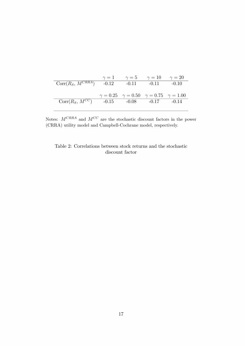
γ = 1 γ = 5 γ = 10 γ = 20Corr(RS, MCRRA) -0.12 -0.11 -0.11 -0.10

γ = 0.25 γ = 0.50 γ = 0.75 γ = 1.00Corr(RS, MCC) -0.15 -0.08 -0.17 -0.14

Notes: MCRRA and MCC are the stochastic discount factors in the power(CRRA) utility model and Campbell-Cochrane model, respectively.

Table 2: Correlations between stock returns and the stochasticdiscount factor

17

Instrument set 1 2 3 4 5 6Power utility

δ 0.995 0.988 0.996 0.990 0.995 0.996(0.020) (0.016) (0.021) (0.018) (0.020) (0.020)

γ 13.219 5.430 17.181 7.181 13.227 15.093(26.602) (10.314) (32.999) (13.280) (26.568) (30.566)

J-test 1.084 6.393 2.321 7.605 3.055 3.364(0.897) (0.603) (0.888) (0.815) (0.802) (0.910)

HJ 0.062 0.071 0.057 0.069 0.062 0.059(0.140) (0.142) (0.139) (0.141) (0.140) (0.140)

rf 2.32% 2.22% 2.35% 2.23% 2.32% 2.28%

Campbell-Cochraneδ 0.952 0.964 0.943 0.963 0.952 0.952

(0.098) (0.060) (0.130) (0.065) (0.096) (0.101)γ 0.664 0.345 0.802 0.368 0.658 0.684

(1.346) (0.761) (1.638) (0.824) (1.321) (1.396)J-test 1.064 5.535 1.977 6.296 3.722 4.031

(0.900) (0.700) (0.922) (0.900) (0.714) (0.854)HJ 0.047 0.064 0.035 0.063 0.047 0.045

(0.137) (0.138) (0.136) (0.137) (0.137) (0.137)rf -0.46% 0.91% -0.62% 0.83% -0.45% -0.57%γ/S 22 16 25 17 22 23

Notes: The Table reports estimates of δ and γ in the power utility andCampbell-Cochrane models using the iterated GMM approach described insection 3, with asymptotic standard errors in parentheses. J-test is Hansen’stest of overidentifying restrictions, computed as in (14), with asymptotic p-value in parenthesis. HJ is the Hansen-Jagannathan specification error mea-sure, computed as in (15), with asymptotic standard error in parenthesis. rfis the real risk-free rate, computed from (3) and (10). S in γ/S is the averagevalue of S over the sample. The instrument sets are:

1: Constant, RS , D/P .2: Constant, RS , D/P , and their lags.3: Constant, RS , RLB, D/P .4. Constant, RS , RLB, D/P , and their lags.5. Constant, RS , D/P , TERM .6. Constant, RS , D/P , TERM , C/C−1.

Table 3: GMM estimation of the power utility and Campbell-Cochranemodels, with returns on stocks and long-term bonds.

18

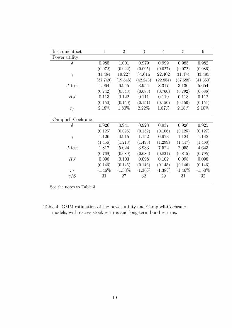
Instrument set 1 2 3 4 5 6Power utility

δ 0.985 1.001 0.979 0.999 0.985 0.982(0.072) (0.022) (0.095) (0.027) (0.072) (0.086)

γ 31.484 19.227 34.616 22.402 31.474 33.495(37.749) (19.845) (42.243) (22.854) (37.688) (41.350)

J-test 1.964 6.945 3.954 8.317 3.136 5.654(0.742) (0.543) (0.683) (0.760) (0.792) (0.686)

HJ 0.113 0.122 0.111 0.119 0.113 0.112(0.150) (0.150) (0.151) (0.150) (0.150) (0.151)

rf 2.18% 1.80% 2.22% 1.87% 2.18% 2.10%

Campbell-Cochraneδ 0.926 0.941 0.923 0.937 0.926 0.925

(0.125) (0.096) (0.132) (0.106) (0.125) (0.127)γ 1.126 0.915 1.152 0.973 1.124 1.142

(1.456) (1.213) (1.493) (1.299) (1.447) (1.468)J-test 1.817 5.624 3.933 7.522 2.955 4.643

(0.769) (0.689) (0.686) (0.821) (0.815) (0.795)HJ 0.098 0.103 0.098 0.102 0.098 0.098

(0.146) (0.145) (0.146) (0.145) (0.146) (0.146)rf -1.46% -1.33% -1.36% -1.38% -1.46% -1.50%γ/S 31 27 32 29 31 32

See the notes to Table 3.

Table 4: GMM estimation of the power utility and Campbell-Cochranemodels, with excess stock returns and long-term bond returns.

19

Instrument set 1 2 3 4 5 6Power utility

δ 0.999 0.993 0.998 0.995 0.999 0.999(0.019) (0.015) (0.025) (0.017) (0.019) (0.021)

γ 15.866 6.448 20.086 8.468 15.866 17.979(23.848) (9.254) (29.556) (11.782) (23.816) (27.379)

J-test 7.090 12.188 11.036 16.519 8.284 16.167(0.420) (0.512) (0.355) (0.622) (0.601) (0.240)

HJ 0.276 0.276 0.277 0.276 0.276 0.276(0.181) (0.179) (0.182) (0.179) (0.181) (0.182)

rf 2.04% 1.90% 2.07% 1.91% 2.04% 2.00%

Campbell-Cochraneδ 0.946 0.964 0.942 0.959 0.946 0.946

(0.099) (0.052) (0.113) (0.065) (0.098) (0.099)γ 0.796 0.401 0.868 0.565 0.792 0.802

(1.267) (0.643) (1.405) (0.887) (1.251) (1.278)J-test 6.524 8.014 13.898 17.940 8.576 12.848

(0.480) (0.843) (0.178) (0.527) (0.573) (0.460)HJ 0.275 0.266 0.279 0.266 0.275 0.276

(0.186) (0.184) (0.187) (0.184) (0.186) (0.186)rf -0.92% 0.47% -1.06% -0.34% -0.92% -0.97%γ/S 25 17 27 21 25 25

See the notes to Table 3.

Table 5: GMM estimation of the power utility and Campbell-Cochranemodels, with returns on stocks, long-term bonds and intermediate-term

bonds.

20

Instrument set 1 2 3 4 5 6Power utility

δ 0.997 1.003 0.993 1.003 0.997 0.995(0.038) (0.019) (0.055) (0.020) (0.038) (0.047)

γ 25.221 13.748 28.573 16.519 25.211 27.212(30.121) (14.713) (34.910) (17.349) (30.077) (33.459)

J-test 6.840 11.567 10.977 16.228 7.881 17.104(0.446) (0.564) (0.359) (0.642) (0.641) (0.195)

HJ 0.277 0.274 0.279 0.274 0.277 0.278(0.184) (0.181) (0.185) (0.181) (0.184) (0.185)

rf 1.82% 1.53% 1.86% 1.58% 1.82% 1.77%

Campbell-Cochraneδ 0.942 0.947 0.939 0.947 0.942 0.941

(0.101) (0.091) (0.114) (0.091) (0.100) (0.102)γ 0.913 0.832 0.964 0.835 0.911 0.932

(1.253) (1.169) (1.384) (1.179) (1.244) (1.273)J-test 6.948 11.647 15.008 21.288 8.647 13.283

(0.434) (0.557) (0.132) (0.321) (0.566) (0.426)HJ 0.279 0.276 0.281 0.276 0.279 0.280

(0.187) (0.187) (0.187) (0.187) (0.187) (0.187)rf -1.40% -1.29% -1.47% -1.37% -1.40% -1.51%γ/S 27 26 28 26 27 28

See the notes to Table 3.

Table 6: GMM estimation of the power utility and Campbell-Cochranemodels, with excess stock returns and returns on long-term bonds and

intermediate-term bonds.

21

86:4 87:4 88:4 89:4 90:4 91:4 92:4 93:4 94:4 95:4 96:4 97:4 98:4 99:4 00:4 01:40

10

20

30

40

50

60

70

80

90

100

110

Figure 1:

Figure 1: Relative risk-aversion γ/St in the Campbell-Cochrane model

22