arX

iv:1

307.

1708

v4 [

mat

h.O

C]

13

Aug

201

3

Piecewise linear approximations of the standard normal first

order loss function

Roberto Rossi,∗,1 S. Armagan Tarim,2 Steven Prestwich,3 Brahim Hnich4

1Business School, University of Edinburgh, Edinburgh, UK

roberto.rossi@ed.ac.uk2Dept. of Management, Hacettepe University, Ankara, Turkey

armagan.tarim@hacettepe.edu.tr3Dept. of Computer Science, University College Cork, Cork, Ireland

s.prestwich@cs.ucc.ie4Dept. of Computer Engineering, Izmir University of Economics, Izmir, Turkey

hnich.brahim@gmail.com

Abstract

The first order loss function and its complementary function are extensively usedin practical settings. When the random variable of interest is normally distributed,the first order loss function can be easily expressed in terms of the standard normalcumulative distribution and probability density function. However, the standardnormal cumulative distribution does not admit a closed form solution and cannotbe easily linearised. Several works in the literature discuss approximations for eitherthe standard normal cumulative distribution or the first order loss function and theirinverse. However, a comprehensive study on piecewise linear upper and lower boundsfor the first order loss function is still missing. In this work, we initially summarisea number of distribution independent results for the first order loss function and itscomplementary function. We then extend this discussion by focusing first on ran-dom variable featuring a symmetric distribution, and then on normally distributedrandom variables. For the latter, we develop effective piecewise linear upper andlower bounds that can be immediately embedded in MILP models. These linearisa-tions rely on constant parameters that are independent of the mean and standarddeviation of the normal distribution of interest. We finally discuss how to computeoptimal linearisation parameters that minimise the maximum approximation error.keywords: first order loss function; complementary first order loss function; piece-wise linear approximation; minimax; Jensen’s; Edmundson-Madansky.Corresponding author: Roberto Rossi, University of Edinburgh Business School,EH8 9JS, Edinburgh, United Kingdom.phone: +44(0)131 6515239email: roberto.rossi@ed.ac.uk

1

1 Introduction

Consider a random variable ω and a scalar variable x. The first order loss function isdefined as

L(x, ω) = E[max(ω − x, 0)], (1)

where E denotes the expected value. The complementary first order loss function isdefined as

L(x, ω) = E[max(x− ω, 0)]. (2)

The first order loss function and its complementary function play a key role in severalapplication domains. In inventory control [10] it is often used to express expected in-ventory holding or shortage costs, as well as service level measures such as the widelyadopted “fill rate”, also known as β service level [1], p. 94. In finance the first orderloss function may be employed to capture risk measures such as the so-called “condi-tional value at risk” (see e.g. [8]). These examples illustrate possible applications of thisfunction. Of course, the applicability of this function goes beyond inventory theory andfinance.

Despite its importance, to the best of our knowledge a comprehensive analysis ofresults concerning the first order loss function seems to be missing in the literature.In Section 2, we first summarise a number of distribution independent results for thefirst order loss function and its complementary function. We then focus on symmetricdistributions and on normal distributions; for these we discuss ad-hoc results in Section3.

According to one of these results, the first order loss function can be expressed interms of the cumulative distribution function of the random variable under scrutiny. De-pending on the probability distribution adopted, integrating this function may constitutea challenging task. For instance, if the random variable is normally distributed, no closedformulation exists for its cumulative distribution function. Several approximations havebeen proposed in the literature, see e.g. [12, 9, 11, 3, 7, 4], which can be employed toapproximate the first order loss function. However, these approximations are generallynonlinear and cannot be easily embedded in mixed integer linear programming (MILP)models.

In Section 4 and 5, we introduce piecewise linear lower and upper bounds for thefirst order loss function and its complementary function for the case of normally dis-tributed random variables. These bounds are based on standard bounding techniquesfrom stochastic programming, i.e. Jensen’s lower bound and Edmundson-Madansky up-per bound [6], p. 167-168. The bounds can be readily used in MILP models and do notrequire instance dependent tabulations. Our linearisation strategy is based on standardoptimal linearisation coefficients computed in such a way as to minimise the maximumapproximation error, i.e. according to a minimax approach. Optimal coefficients for ap-proximations comprising from two to eleven segments will be presented in Table 1; thesecan be reused to approximate the loss function associated with any normally distributedrandom variable.

2

2 The first order loss function and its complementary func-

tion

Consider a continuous random variable ω with support over R, probability density func-tion gω(x) : R → (0, 1) and cumulative distribution function Gω(x) : R → (0, 1). Thefirst order loss function can be rewritten as

L(x, ω) =

∫ ∞

−∞max(t− x, 0)gω(t) dt =

∫ ∞

x(t− x)gω(t) dt. (3)

The complementary first order loss function can be rewritten as

L(x, ω) =

∫ ∞

−∞max(x− t, 0)gω(t) dt =

∫ x

−∞(x− t)gω(t) dt. (4)

Lemma 1. The first order loss function L(x, ω) can also be expressed as

L(x, ω) =

∫ ∞

x(1−Gω(t)) dt (5)

Proof.

L(x, ω) =

∫ ∞

x(t− x)gω(t) dt (6)

=

∫ ∞

xtgω(t) dt− x

∫ ∞

xgω(t) dt (7)

the integration of ∫ ∞

xtgω(t) dt

is a well-known integration by parts that proceeds as follows. Let u(t) = t, u′(t) = 1,v(t) = −(1−Gω(t)), v′(t) = gω(t). Rewrite the integral as

∫ b

xtgω(t) dt = [−t(1−Gω(t))]bx +

∫ b

x(1−Gω(t)) dt

and take the limit since b → ∞. The product term in the integration by parts formulaconverges to x(1−Gω(x)) as b→∞. We therefore take the limit to obtain the identity

∫ ∞

xtgω(t) dt = x(1−Gω(x)) +

∫ ∞

x(1−Gω(t)) dt

and by substituting∫∞x tgω(t) dt with this expression we obtain

L(x, ω) = x(1−Gω(x)) +

∫ ∞

x(1−Gω(t)) dt − x(1−Gω(x)) (8)

=

∫ ∞

x(1−Gω(t)) dt (9)

3

The following well-known lemma is introduced, together with its proof, for complete-ness.

Lemma 2. The complementary first order loss function L(x, ω) can also be expressedas

L(x, ω) =

∫ x

−∞Gω(t) dt. (10)

Proof.

L(x, ω) =

∫ x

−∞(x− t)gω(t) dt (11)

= x

∫ x

−∞gω(t) dt−

∫ x

−∞tgω(t) dt (12)

= xGω(x)−∫ x

−∞tgω(t) dt (13)

= xGω(x)− xGω(x) +

∫ x

−∞Gω(t) dt (14)

=

∫ x

−∞Gω(t) dt (15)

There is a close relationship between the first order loss function and the comple-mentary first order loss function.

Lemma 3. The first order loss function L(x, ω) can also be expressed as

L(x, ω) = L(x, ω)− (x− ω) (16)

where ω = E[ω].

Proof.

L(x, ω) =

∫ ∞

x(t− x)gω(t) dt (17)

=

∫ ∞

xtgω(t) dt− x

∫ ∞

xgω(t) dt (18)

=

∫ ∞

−∞tgω(t) dt−

∫ x

−∞tgω(t) dt− x

∫ ∞

xgω(t) dt (19)

=

∫ ∞

−∞tgω(t) dt−

∫ x

−∞tgω(t) dt− x(1−Gω(t)) (20)

=

∫ ∞

−∞tgω(t) dt− xGω(x) +

∫ x

−∞Gω(t) dt− x(1−Gω(t)) (21)

=

∫ x

−∞Gω(t) dt− (x− ω) (22)

= L(x, ω)− (x− ω) (23)

4

Because of the relation discussed in Lemma 3, in what follows without loss of gener-ality most of the results will be presented for the complementary first order loss function.

Another known result for the first order loss function and its complementary functionis their convexity, which we present next.

Lemma 4. L(x, ω) and L(x, ω) are convex in x.

Proof. We shall prove the result for L(x, ω). Recall that L(x, ω) =∫ x−∞Gω(t) dt. From

the fundamental theorem of integral calculus

d

dxL(x, ω) = Gω(x)

andd2

dx2L(x, ω) = gω(x).

Since gω(x) is nonnegative the result follows immediately; furthermore, the proof forL(x, ω) follows from Lemma 3 and from the fact that −x is convex.

For a random variable ω with symmetric probability density function, we introducethe following results.

Lemma 5. If the probability density function of ω is symmetric about a mean value ω,then

L(x, ω) = L(2ω − x, ω).

Proof.

L(x, ω) =

∫ ∞

x(1−Gω(t)) dt (24)

=

∫ ω−(x−ω)

−∞Gω(t) dt (25)

= L(2ω − x, ω) (26)

Lemma 6. If the probability density function of ω is symmetric about a mean value ω,then

L(x, ω) = L(2ω − x, ω) + (x− ω)

andL(x, ω) = L(2ω − x, ω)− (x− ω).

Proof. Follows immediately from Lemma 3 and Lemma 5.

The results presented so far are easily extended to the case in which the randomvariable is discrete. In the following section we present results for the case in which therandom variable is normally distributed.

5

3 The first order loss function for a normally distributed

random variable

Let ζ be a normally distributed random variable with mean µ and standard deviationσ. Recall that the Normal probability density function is defined as

gζ(x) =1

σ√

2πe−

(x−µ)2

2σ2 . (27)

No closed form expression exists for the cumulative distribution function

Gζ(x) =

∫ x

−∞gζ(x) dx.

Let φ(x) be the standard Normal probability density function and Φ(x) the respectivecumulative distribution function.

We next present three known results for a normally distributed random variable: astandardisation result in Lemma 7, and two closed form expressions for the computationof the loss function and of its complementary function in Lemmas 8 and 9.

Lemma 7. The complementary first order loss function of ζ can be expressed in termsof the standard Normal cumulative distribution function as

L(x, ζ) = σ

∫ x−µ

σ

−∞Φ(t) dt = σL

(x− µ

σ,Z

), (28)

where Z is a standard Normal random variable.

Proof. Recall that the complementary first order loss function is defined as

L(x, ζ) =

∫ x

−∞(x− t)gζ(t) dt.

We change the upper integration limit to

f(x) =x− µ

σ

by noting that

f−1(y) = σy + µ,df−1(y)

dy= σ

it follows that

L(x, ζ) =

∫ f(x)

−∞(x− f−1(t))gζ(f−1(t))

df−1(t)

dtdt. (29)

= σ

∫ x−µσ

−∞(x− σt− µ)

1

σφ(t) dt. (30)

= σ

∫ x−µ

σ

−∞σ

(x− µ

σ− t

)1

σφ(t) dt. (31)

6

Lemma 8. The complementary first order loss function L(x, ζ) can be rewritten inclosed form as

L(x, ζ) = σ

(φ

(x− µ

σ

)+ Φ

(x− µ

σ

)x− µ

σ

)

Proof. Integrate by parts Eq. 28 and observe that∫ x−µ

σ−∞ tφ(t) dt = −φ(x−µ

σ ).

From Lemma 3 the first order loss function of ζ can be expressed as

L(x, ζ) = −(x− µ) + σ

∫ x−µ

σ

−∞Φ(t) dt (32)

Recall that an alternative expression is obtained via Lemma 1,

L(x, ζ) = σ

∫ ∞

x−µ

σ

(1− Φ(t)) dt. (33)

From Lemma 3 and Lemma 8 we obtain the closed form expression

L(x, ζ) = −(x− µ) + σ

(φ

(x− µ

σ

)+ Φ

(x− µ

σ

)x− µ

σ

)(34)

Lemma 9. The first order loss function L(x, ζ) can be rewritten in closed form as

L(x, ζ) = σ

(φ

(x− µ

σ

)−(

1− Φ

(x− µ

σ

))x− µ

σ

)

Proof. Integrate by parts Eq. 32 and observe that∫∞

x−µ

σ

tφ(t) dt = φ(x−µσ ).

Furthermore, since the Normal distribution is symmetric, both Lemma 5 and Lemma6 hold.

4 Jensen’s lower bound for the standard normal first order

loss function

We introduce a well-known inequality from stochastic programming [6], p. 167.

4.1 Jensen’s lower bound

Theorem 1 (Jensen’s inequality). Consider a random variable ω with support Ω and afunction f(x, s), which for a fixed x is convex for all s ∈ Ω, then

E[f(x, ω)] ≥ f(x,E[ω]).

Proof. [2], p. 140.

7

Common discrete lower bounding approximations in stochastic programming areextensions of Jensen’s inequality. The usual strategy is to find a low cardinality discreteset of realisations representing a good approximation of the true underling distribution.[2], p. 288, discuss one of these discrete lower bounding approximations which consistsin partitioning the support Ω into a number of disjoint regions, Jensen’s bound is thenapplied in each of these regions.

More formally, let gω(·) denote the probability density function of ω and considera partition of the support Ω of ω into N disjoint compact subregions Ω1, . . . ,ΩN . Wedefine, for all i = 1, . . . , N

pi = Prω ∈ Ωi =

∫

Ωi

gω(t) dt

and

E[ω|Ωi] =1

pi

∫

Ωi

tgω(t) dt

Theorem 2.

E[f(x, ω)] ≥N∑

i=1

pif(x,E[ω|Ωi])

Proof. [2], p. 289.

Theorem 3. Given a random variable ω Jensen’s bound (Theorem 1) is applicable tothe first order loss function L(x, ω) and its complementary function L(x, ω).

Proof. Follows immediately from Lemma 4.

Having established this result, we must then decide how to partition the support ωin order to obtain a good bound. In fact, to generate good lower bounds, it is necessaryto carefully select the partition of the support ω. The optimal partitioning strategy willdepend, of course, on the probability distribution of the random variable ω.

4.2 Minimax discrete lower bounding approximation

We discuss a minimax strategy for generating discrete lower bounding approximations ofthe (complementary) first order loss function. In this strategy, we partition the support ωinto a predefined number of regions N in order to minimise the maximum approximationerror.

Consider a random variable ω and the associated complementary first order lossfunction

L(x, ω) = E[max(x− ω, 0)];

assume that the support Ω of ω is partitioned into N disjoint subregions Ω1, . . . ,ΩN .

Lemma 10. For the (complementary) first order loss function the lower bound presentedin Theorem 2 is a piecewise linear function with N + 1 segments.

8

Proof. Consider the bound presented in Theorem 2 and let f(x, ω) = max(x− ω, 0),

Llb(x, ω) =N∑

i=1

pi max(x− E[ω|Ωi], 0)

this function is equivalent to

Llb(x, ω) =

0 −∞ ≤ x ≤ E[ω|Ω1]p1x− p1E[ω|Ω1] E[ω|Ω1] ≤ x ≤ E[ω|Ω2](p1 + p2)x− (p1E[ω|Ω1] + p2E[ω|Ω2]) E[ω|Ω2] ≤ x ≤ E[ω|Ω3]...

...(p1 + p2 + . . .+ pN )x− (p1E[ω|Ω1] + p2E[ω|Ω2] + . . .+ pNE[ω|ΩN ]) E[ω|ΩN−1] ≤ x ≤ E[ω|ΩN ]

which is piecewise linear in x with breakpoints at E[ω|Ω1],E[ω|Ω2], . . . ,E[ω|ΩN ]. Theproof for the first order loss function follows a similar reasoning.

Lemma 11. Consider the i-th linear segment of Llb(x, ω)

Lilb(x, ω) = x

i∑

k=1

pk −i∑

k=1

pkE[ω|Ωk] E[ω|Ωi] ≤ x ≤ E[ω|Ωi+1],

where i = 1, . . . , N . Let Ωi = [a, b], then Lilb(x, ω) is tangent to L(x, ω) at x = b.

Furthermore, the 0-th segment x = 0 is tangent to L(x, ω) at x = −∞.

Proof. Note that

Lilb(x, ω) = xi∑

k=1

∫

Ωk

gω(t) dt−i∑

k=1

∫

Ωk

tgω(t) dt

and thatΩ1 ∪ Ω2 ∪ . . . ∪ Ωi =)−∞, b]

it follows

Lilb(x, ω) = x

∫ b

−∞gω(t) dt−

∫ b

−∞tgω(t) dt

and

Lilb(x, ω) = Gω(b)(x − b) +

∫ b

−∞Gω(t) dt.

which is the equation of the tangent line to L(x, ω) at a given point b, that is

y = L(b, ω)′(x− b) + L(b, ω).

x = 0 is tangent to L(x, ω) at x = −∞ since L(x, ω) is convex, positive and

limx→−∞

L(x, ω) = 0.

The very same reasoning can be easily applied to the first order loss function.

9

Lemma 12. The maximum approximation error between Llb(x, ω) and L(x, ω) will beattained at a breakpoint.

Proof. By recalling that L(x, ω) is convex (Lemma 4), since Llb(x, ω) is piecewise linear(Lemma 10) and each segment of Llb(x, ω) is tangent to L(x, ω) (Lemma 11), it followsthat the maximum error will be attained at a breakpoint.

Theorem 4. Given the number of regions N , Ω1, . . . ,ΩN is an optimal partition ofthe support Ω of ω under a minimax strategy, if and only if approximation errors atbreakpoints are all equal.

Proof. The approximation errors for x → −∞ and x → ∞ are both 0; since we haveN+1 segments, we only have N breakpoints to check.

We first show that (→) if Ω1, . . . ,ΩN is an optimal partition of the support Ω of ωunder a minimax strategy, then approximation errors at breakpoints are all equal.

A first observation that follows immediately from Lemma 12 is that, if the slopeof segment Li+1

lb (x, ω) remains unchanged, and the breakpoint between Lilb(x, ω) and

Li+1lb (x, ω) moves towards the point at which Li+1

lb (x, ω) is tangent to L(x, ω), the errorat such breakpoint decreases.

If one changes the size of region Ωi so that the upper limit becomes bi + ∆, thenE[ω|Ωi] will increase if ∆ > 0, or will decrease if ∆ < 0. This immediately follows fromthe definition of E[ω|Ωi]. Therefore, the breakpoint between segment i and segment i+1,which occurs at E[ω|Ωi], will move accordingly. However, the slope of segment i + 1,which we recall is equal to Gω(bi+1), depends uniquely on the upper limit of the regionΩi+1, bi+1, and is not affected by a change in the upper limit of region Ωi. Therefore,the error at the breakpoint between segment i and segment i + 1 will decrease if ∆ > 0,or will increase if ∆ < 0.

Now, assume that Ω1, . . . ,ΩN is an optimal partition of the support Ω of ω andapproximation errors at breakpoints are not all equal. Furthermore, assume that themaximum approximation error occurs at breakpoint i. By increasing the size of theregion Ωi, i.e. by setting the upper limit to bi + ∆, where ∆ > 0, it is possible todecrease the maximum error until it becomes equal to the error at breakpoint k, wherek ∈ 1, . . . , i − 1. The procedure can be repeated until all approximation errors areequal.

Second, we show that (←) if approximation errors at breakpoints are all equal, thenΩ1, . . . ,ΩN is an optimal partition of the support Ω of ω under a minimax strategy.

If approximation errors at breakpoints are all equal and we change the size of regionΩi by setting the upper limit to bi + ∆, where ∆ > 0, then the approximation errorat breakpoint i − 1 will increase; conversely, if ∆ < 0, then the approximation error atbreakpoint i + 1 will increase.

By using this last result it is possible to derive a set of equations that can be solvedfor computing an optimal partitioning. Let us consider the error ei at breakpoint i, thiscan be expressed as

ei = L(E[ω|Ωi], ω)− Lilb(E[ω|Ωi], ω),

10

where Ωi = [ai, bi]. Since we have N breakpoints to check, we must solve a systemcomprising the following N − 1 equations

e1 = ei for i = 2, . . . , N.

under the following restrictions

a1 = −∞bN =∞ai ≤ bi for i = 1, . . . , Nbi = ai+1 for i = 1, . . . , N − 1

The system therefore involves N − 1 variables, each of which identifies the boundarybetween two disjoint regions Ωi and Ωi+1.

Theorem 5. Assume that the probability density function of ω is symmetric about amean value ω. Then, under a minimax strategy, if Ω1, . . . ,ΩN is an optimal partition ofthe support Ω of ω, breakpoints will be symmetric about ω.

Proof. This follows from Lemma 6 and Theorem 4.

In this case, by exploiting the symmetry of the piecewise linear approximation, anoptimal partitioning can be derived by solving a smaller system comprising ⌈N/2⌉ equa-tions, where N is the number of regions Ωi and ⌈x⌉ rounds x to the next integer value.

Unfortunately, equations in the above system are nonlinear and do not admit a closedform solution in the general case.

4.2.1 Normal distribution

We will next discuss the system of equations that leads to an optimal partitioning forthe case of a standard Normal random variable Z. This partitioning leads to a piecewiselinear approximation that is, in fact, easily extended to the general case of a normallydistributed variable ζ with mean µ and standard deviation σ via Lemma 7. This equationsuggests that the error of this approximation is independent of µ and proportional to σ.

Consider a partitioning for the support Ω of Z into N adjacent regions Ωi = [ai, bi],where i = 1, . . . , N . From Theorem 5, if N is odd, then b⌈N/2⌉ = 0 and bi = −bN+1−i, if

N is even, then bi = −bN+1−i. We shall use Lemma 8 for expressing L(x,Z). Then, byobserving that ∫ bi

ai

tφ(t) dt = φ(ai)− φ(bi)

and that p1 + p2 + . . . + pi = Φ(bi), we rewrite

Lilb(E[Z|Ωi], Z) = Φ(bi)E[Z|Ωi]−i∑

k=1

(φ(ai)− φ(bi)) (35)

= Φ(bi)E[Z|Ωi]− (φ(a1)− φ(bi)) (36)

= Φ(bi)E[Z|Ωi] + φ(bi) (37)

11

To express the conditional expectation E[Z|Ωi] we proceed as follows: let pi = Φ(bi)−Φ(ai), it follows

E[Z|Ωi] =φ(ai)− φ(bi)

Φ(bi)− Φ(ai).

To solve the above system of non-linear equations we will exploit the close connectionsbetween finding a local minimum and solving a set of nonlinear equations. In particular,we will use the Gauss-Newton method to find a partition Ω1, . . . ,ΩN of the support ofZ that minimises the following sum of squares

N∑

k=2

(e1 − ek)2

This minimisation problem can be solved by software packages such as Mathematica(see NMinimize).

4.2.2 Numerical examples

The classical Jensen’s bound for the complementary first order loss function of a standardNormal random variable Z is show in Fig. 1. This is obtained by considering a degeneratepartition of the support of Z comprising only a single region Ω1 = [−∞,∞]. In practice,we simply replace Z by its expected value, i.e. zero. Therefore we simply have Llb =max(x, 0). The maximum error of this piecewise linear approximation occurs for x = 0and it is equal to 1/

√2π.

-2 -1 1 2x

0.5

1.0

1.5

2.0

L`Hx,ZL-L

`lbHx,ZL

L`

lbHx,ZL

L`Hx,ZL

Figure 1: classical Jensen’s bound for L(x,Z)

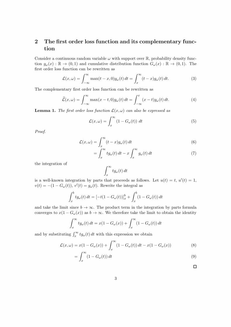
If we split the support of Z into four regions (Fig. 2), the solution to the system ofnonlinear equations prescribes to split Ω at b1 = −0.886942, b2 = 0, b3 = 0.886942. Themaximum error is 0.0339052 and it is observed at x ∈ ±1.43535,±0.415223.

12

-2 -1 1 2x

0.5

1.0

1.5

2.0

L`Hx,ZL-L

`lbHx,ZL

L`

lbHx,ZL

L`Hx,ZL

Figure 2: five-segment piecewise Jensen’s bound for L(x,Z)

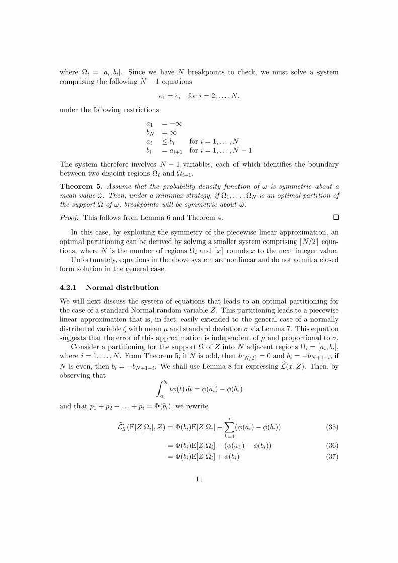
In Table 1 we report parameters of Llb(x,Z) with up to eleven segments. In Fig. 3we present the approximation error of Llb(x,Z) with up to eleven segments.

4 6 8 10Number of segments

0.1

0.2

0.3

0.4

Absolute error

Figure 3: approximation error of Llb(x,Z) with up to eleven segments

13

Piecewise linear approximation parametersSegments Error i 1 2 3 4 5 6 7 8 9 10

2 0.398942

bi ∞pi 1E[ω|Ωi] 0

3 0.120656

bi 0 ∞pi 0.5 0.5E[ω|Ωi] −0.797885 0.797885

4 0.0578441

bi −0.559725 0.559725 ∞pi 0.287833 0.424333 0.287833E[ω|Ωi] −1.18505 0 1.18505

5 0.0339052

bi −0.886942 0 0.886942 ∞pi 0.187555 0.312445 0.312445 0.187555E[ω|Ωi] −1.43535 −0.415223 0.415223 1.43535

6 0.0222709

bi −1.11507 −0.33895 0.33895 1.11507 ∞pi 0.132411 0.234913 0.265353 0.234913 0.132411E[ω|Ωi] −1.61805 −0.691424 0 0.691424 1.61805

7 0.0157461

bi −1.28855 −0.579834 0 0.579834 1.28855 ∞pi 0.0987769 0.182236 0.218987 0.218987 0.182236 0.0987769E[ω|Ωi] −1.7608 −0.896011 −0.281889 0.281889 0.896011 1.7608

8 0.0117218

bi −1.42763 −0.765185 −0.244223 0.244223 0.765185 1.42763 ∞pi 0.0766989 0.145382 0.181448 0.192942 0.181448 0.145382 0.0766989E[ω|Ωi] −1.87735 −1.05723 −0.493405 0 0.493405 1.05723 1.87735

9 0.00906529

bi −1.54317 −0.914924 −0.433939 0 0.433939 0.914924 1.54317 ∞pi 0.0613946 0.118721 0.152051 0.167834 0.167834 0.152051 0.118721 0.0613946E[ω|Ωi] −1.97547 −1.18953 −0.661552 −0.213587 0.213587 0.661552 1.18953 1.97547

10 0.00721992

bi −1.64166 −1.03998 −0.58826 −0.19112 0.19112 0.58826 1.03998 1.64166 ∞pi 0.0503306 0.0988444 0.129004 0.146037 0.151568 0.146037 0.129004 0.0988444 0.0503306E[ω|Ωi] −2.05996 −1.30127 −0.8004 −0.384597 0. 0.384597 0.8004 1.30127 2.05996

11 0.00588597

bi −1.72725 −1.14697 −0.717801 −0.347462 0. 0.347462 0.717801 1.14697 1.72725 ∞pi 0.0420611 0.0836356 0.110743 0.127682 0.135878 0.135878 0.127682 0.110743 0.0836356 0.0420611E[ω|Ωi] −2.13399 −1.39768 −0.9182 −0.526575 −0.17199 0.17199 0.526575 0.9182 1.39768 2.13399

Table 1: parameters of Llb(x,Z) with up to eleven segments

14

In Fig. 4 we exploited Lemma 7 to obtain the five-segment piecewise Jensen’s boundfor L(x, ζ), where ζ is a normally distributed random variable with mean µ = 20 andstandard deviation σ = 5. The maximum error is σ0.0339052 and it is observed atx ∈ σ(±1.43535) + µ, σ(±0.415223) + µ.

15 20 25 30x

2

4

6

8

10

L`Hx,ΖL-L

`lbHx,ΖL

L`

lbHx,ΖL

L`Hx,ΖL

Figure 4: five-segment piecewise Jensen’s bound for L(x, ζ), where µ = 20 and σ = 5

5 An approximate piecewise linear upper bound for the

standard normal first order loss function

In this section we introduce a simple bounding technique that exploits convexity of the(complementary) first order loss function to derive a piecewise linear upper bound.

5.1 A piecewise linear upper bound

Without loss of generality we shall introduce the bound for the complementary firstorder loss function. Consider a random variable ω with support Ω. From Lemma 4,L(x, ω) is convex in x regardless of the distribution of ω. Given an interval [a, b] ∈ R, it ispossible to construct an upper bound by exploiting the very same definition of convexity,that is by constructing a straight line Lub(x, ω) between the two points (a, L(a, ω)) and(b, L(b, ω)). The slope (α) and the intercept (β) of this line can be easily computed

α =L(b, ω)− L(a, ω)

b− a, β =

bL(a, ω) − aL(b, ω)

b− a.

15

The upper bound is then

Lub(x, ω) = αx + β a ≤ x ≤ b (38)

= L(a, ω)b− x

b− a+ L(b, ω)

x − a

b − aa ≤ x ≤ b (39)

We can improve the quality of this bound by partitioning the domain R of L(x, ω) intoN disjoint regions Di = [ai, bi], i = 1, . . . , N . The selected regions must be all compactand adjacent. Because of the convexity of L(x, ω) the bound can be then applied to eachof these regions considered separately.

However, since L(x, ω) is defined over R, it is not possible to guarantee a completecovering of the domain by using compact regions. We must therefore add two extremeregions D0 = [−∞, a1] and DN+1 = [aN+1 = bN ,∞] to ensure the one obtained is indeedan upper bound for each x ∈ R. By noting that

limx→−∞

L(x, ω) = 0 and limx→∞

L(x, ω) = x

it is easy to derive equations for the lines associated with these two extra regions. Inparticular, we associate with D0 a horizontal line with slope α = 0 and intercept β =L(a1, ω), and with DN+1 a line with slope α = 1 and intercept β = L(bN , ω)− bN .

Also in this case, we must then decide how to partition the domain R into N + 2intervals D0, . . . ,DN+1 to obtain a tight bound. Once more, the optimal partitioningstrategy will depend on the probability distribution of the random variable ω.

5.2 Minimax piecewise linear upper bound

We discuss a minimax strategy for generating a piecewise linear upper bound of the(complementary) first order loss function L(x, ω). In this strategy, we partition of thedomain R of x into a predefined number of regions N + 2 in order to minimise themaximum approximation error. Note that, since this domain is not compact, one needsat least two regions to derive a piecewise linear upper bound.

Consider a random variable ω and the associated complementary first order lossfunction

L(x, ω) = E[max(x− ω, 0)];

assume that the domain R of x is partitioned into N + 2 disjoint adjacent subregionsD0, . . . ,DN+1, where D0 = [−∞, a1], Di = [ai, bi], for i = 1, . . . , N , and DN+1 = [bN ,∞],and consider the following piecewise linear upper bound

Lub(x, ω) =

L(a1, ω) x ∈ D0...

L(ai, ω) bi−xbi−ai

+ L(bi, ω) x−aibi−ai

x ∈ Di

...

x + L(bN , ω)− bN x ∈ DN+1

Let Liub(x, ω) be the linear segment of Lub(x, ω) over Di, for i = 0, . . . , N + 1.

16

Lemma 13. Consider Liub(x, ω), where i = 1, . . . , N ; the maximum approximation error

between Liub(x, ω) and L(x, ω) will be attained for

xi = G−1ω

(L(bi, ω)− L(ai, ω)

bi − ai

).

Proof. The idea here is to derive a line that is tangent to L(x, ω) and that has a slopeequal to that of the i-th linear segment of Lub(x, ω). We have already discussed inLemma 11 that the equation of the tangent to L(x, ω) at a given point xi is

y = L(xi, ω)′(x− p) + L(xi, ω)

that is

Lilb(x, ω) = Gω(xi)(x− p) +

∫ xi

−∞Gω(t) dt.

The slope Gω(xi) only depends on xi. To find a tangent with a slope equal to that ofthe i-th linear segment of Lub(x, ω), we simply let

Gω(xi) =L(bi, ω)− L(ai, ω)

bi − ai

and invert the cumulative distribution function.

Note that the maximum approximation error for the linear segment over D0 isL(a1, ω) and the maximum approximation error for the linear segment over DN+1 isL(bN , ω)−bN . This can be inferred from the fact that L(x, ω) monotonically approaches0 for x→ −∞ and x for x→∞.

Theorem 6. D0, . . . ,DN+1 is an optimal partition under a minimax strategy, if andonly if the maximum approximation error between L(x, ω) and each linear segment ofLub(x, ω) is the same.

Proof. The proof of this theorem can be obtained from Lemma 13 and from Theorem4. In particular, the key insight needed to understand this result is the following. InTheorem 4 we showed that the approximation errors at breakpoints for the piecewiselinear lower bound presented are all equal to each other and also equal to the maximumapproximation error; furthermore, in Lemma 11 we showed that the i-th piecewise linearsegment of this lower bound agrees with the original function at point bi, where Ωi =[ai, bi] is the i-th partition of the support of Z, for i = 1, . . . , N . Since the first orderloss function is convex and we know the maximum approximation error, by shiftingup the piecewise linear lower bound by a value equal to the maximum approximationerror we immediately obtain a piecewise linear upper bound comprising N +1 segments.This upper bound agrees with the original function at E[Z|Ωi], for i = 1, . . . , N . Themaximum approximation error will be attained at those points in which the lower boundwas tangent to the original function, that is a1, b1, b2, . . . , bN . By using a reasoningsimilar to the one developed for Theorem 4, it is possible to show that, if we increase ordecrease at least one E[Z|Ωi], the maximum approximation error can only increase.

17

By using this result it is possible to derive a set of equations that can be solved forcomputing an optimal partitioning. Let us consider the maximum approximation errorei associated with the i-th linear segment of Lub(x, ω), this can be expressed as

ei = Liub(xi, ω)− L(xi, ω),

where i = 1, . . . , N ; furthermore e0 = L(a1, ω) and eN+1 = L(bN , ω) − bN . Since wehave N + 2 segments to check, we must solve a system comprising the following N + 1equations

e0 = ei for i = 1, . . . , N + 1

under the following restrictions

ai ≤ bi for i = 1, . . . , Nbi = ai+1 for i = 1, . . . , N − 1

The system involves N + 1 variables, each of which identifies the boundary between twodisjoint adjacent regions Di and Di+1.

Theorem 7. Assume that the probability density function of ω is symmetric about amean value ω. Then, under a minimax strategy, if D0, . . . ,DN+1 is an optimal partitionof the domain, breakpoints will be symmetric about the mean value ω.

Proof. This follows from Lemma 6 and Theorem 6.

In this case, by exploiting the symmetry of the piecewise linear approximation, anoptimal partitioning can be derived by solving a smaller system comprising ⌈(N + 1)/2⌉equations, where N + 2 is the number of regions Di and ⌈x⌉ rounds x to the next integervalue.

As in the case of Jensen’s bound, equations in the above system are nonlinear anddo not admit a closed form solution in the general case. For sake of completeness, wewill briefly discuss next how to derive the system of nonlinear equations for the case ofa standard normal random variable Z. However, one should note that in practice, byexploiting the properties illustrated in the proof of Theorem 6, one does not need tosolve a new system of nonlinear equations to derive the piecewise linear upper bound.All information needed, i.e. maximum approximation error at breakpoints and locationsof the breakpoint, are in fact immediately available as soon as the system of equationpresented for the piecewise linear lower bound is solved (Table 1).

The upper bound presented is closely related to a well-known inequality from stochas-tic programming, see e.g. [6], p. 168, [5], p. 316, and [2], pp. 291-293. As pointed outin [6], p. 168, Edmundson-Madanski’s upper bound can be seen as a bound where theoriginal distribution is replaced by a two point distribution and the problem itself isunchanged, or it can be viewed as a bound where the distribution is left unchanged andthe original function is replaced by a linear affine function represented by a straight line.The above discussion clearly demonstrates the dual nature of this upper bound.

18

5.3 Normal distribution

We will next discuss the system of equations that leads to an optimal partitioning forthe case of a standard Normal random variable Z. This partitioning leads to a piecewiselinear approximation that is, in fact, easily extended to the general case of a normallydistributed variable ζ with mean µ and standard deviation σ via Lemma 7. Also forthis second approximation this equation suggests that the error is independent of µ andproportional to σ.

Consider a partitioning for the domain of x in L(x, ω) into N + 2 adjacent regionsDi = [ai, bi], where i = 0, . . . , N + 1. From Theorem 7, if N is odd, then b⌈N/2⌉ = 0 andbi = −bN+1−i, if N is even, then bi = −bN+1−i. Also in this case, we shall use Lemma 8for expressing L(x,Z), and we will exploit the close connections between finding a localminimum and solving a set of nonlinear equations. We will therefore use the Gauss-Newton method to minimize the following sum of squares

N+1∑

k=1

(e0 − ek)2

This minimisation problem can be solved by software packages such as Mathematica(see NMinimize).

5.3.1 Numerical examples

A two-segment piecewise linear upper bound for the complementary first order lossfunction of a standard Normal random variable Z is shown in Fig. 5. This bound hasbeen obtained, under the minimax criterion previously described, by considering a singlebreakpoint in the domain, i.e. x = 0. Of course, the maximum error of this piecewiselinear approximation occurs for x = ±∞ and it is equal to 1/

√2π. It is easy to observe

that this upper bound can be obtained by adding to the classical Jensen’s lower boundpresented in Fig. 1 a constant value equal to its maximum approximation error, i.e.1/√

2π.We next present a more interesting case, in which the domain has been split into

five regions (Fig. 6). Breakpoints are positioned at x ∈ ±1.43535,±0.415223. Thesewere the locations at which the maximum error, i.e. 0.0339052, was observed in Fig.2. Also in this case, the five-segment piecewise linear upper bound can be obtained byadding to the five-segment piecewise Jensen’s lower bound a value equal to its maximumapproximation error.

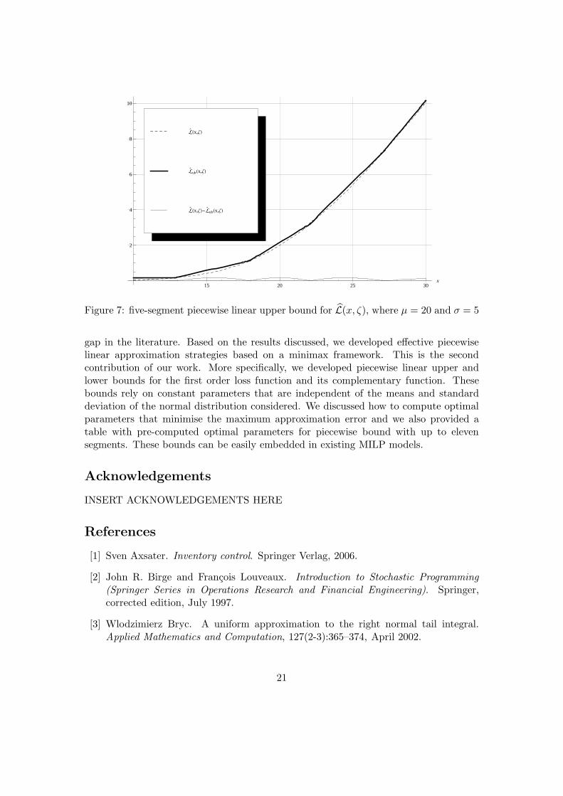
Finally, in Fig. 7, we show an example in which we exploited Lemma 7 to obtain,from the approximation presented in Fig. 6, the five-segment piecewise linear upperbound for L(x, ζ), where ζ is a normally distributed random variable with mean µ = 20and standard deviation σ = 5. The maximum error is σ0.0339052 and it is observed atx ∈ ±∞, σ(±0.886942) + µ, µ.

19

-2 -1 1 2x

0.5

1.0

1.5

2.0

L`Hx,ZL-L

`ubHx,ZL

L`

ubHx,ZL

L`Hx,ZL

Figure 5: two-segment piecewise linear upper bound for L(x,Z)

-2 -1 1 2x

0.5

1.0

1.5

2.0

L`Hx,ZL-L

`ubHx,ZL

L`

ubHx,ZL

L`Hx,ZL

Figure 6: five-segment piecewise linear upper bound for L(x,Z)

6 Conclusions

We summarised a number of distribution independent results for the first order lossfunction and its complementary function. We then focused on symmetric distributionsand on normal distributions; for these we discussed ad-hoc results. To the best of ourknowledge a comprehensive analysis of results concerning the first order loss functionseems to be missing in the literature. The first contribution of this work was to fill this

20

15 20 25 30x

2

4

6

8

10

L`Hx,ΖL-L

`ubHx,ΖL

L`

ubHx,ΖL

L`Hx,ΖL

Figure 7: five-segment piecewise linear upper bound for L(x, ζ), where µ = 20 and σ = 5

gap in the literature. Based on the results discussed, we developed effective piecewiselinear approximation strategies based on a minimax framework. This is the secondcontribution of our work. More specifically, we developed piecewise linear upper andlower bounds for the first order loss function and its complementary function. Thesebounds rely on constant parameters that are independent of the means and standarddeviation of the normal distribution considered. We discussed how to compute optimalparameters that minimise the maximum approximation error and we also provided atable with pre-computed optimal parameters for piecewise bound with up to elevensegments. These bounds can be easily embedded in existing MILP models.

Acknowledgements

INSERT ACKNOWLEDGEMENTS HERE

References

[1] Sven Axsater. Inventory control. Springer Verlag, 2006.

[2] John R. Birge and Francois Louveaux. Introduction to Stochastic Programming(Springer Series in Operations Research and Financial Engineering). Springer,corrected edition, July 1997.

[3] Wlodzimierz Bryc. A uniform approximation to the right normal tail integral.Applied Mathematics and Computation, 127(2-3):365–374, April 2002.

21

[4] Steven K. De Schrijver, El-Houssaine Aghezzaf, and Hendrik Vanmaele. Double pre-cision rational approximation algorithm for the inverse standard normal first orderloss function. Applied Mathematics and Computation, 219(3):1375–1382, October2012.

[5] Karl Frauendorfer and Michael Schurle. Stochastic linear programs with recourseand arbitrary multivariate distributions. In Christodoulos A Floudas and Panos MPardalos, editors, Encyclopedia of Optimization, pages 2488–2493. Springer US,2001.

[6] Peter Kall and Stein W. Wallace. Stochastic Programming (Wiley InterscienceSeries in Systems and Optimization). John Wiley & Sons, August 1994.

[7] Jean M. Linhart. Algorithm 885: Computing the logarithm of the normal distribu-tion. ACM Trans. Math. Softw., 35(3), October 2008.

[8] Renata Mansini, W lodzimierz Ogryczak, and Maria Grazia Speranza. Conditionalvalue at risk and related linear programming models for portfolio optimization.Annals of Operations Research, 152(1):227–256, July 2007.

[9] Haim Shore. Simple approximations for the inverse cumulative function, the densityfunction and the loss integral of the normal distribution. Journal of the RoyalStatistical Society. Series C (Applied Statistics), 31(2):pp. 108–114, 1982.

[10] Edward A. Silver, David F. Pyke, and Rein Peterson. Inventory Management andProduction Planning and Scheduling. John-Wiley and Sons, New York, 1998.

[11] Gary R. Waissi and Donald F. Rossin. A sigmoid approximation of the standardnormal integral. Applied Mathematics and Computation, pages 91–95, June 1996.

[12] Marvin Zelen and Norman C. Severo. Probability functions. In Milton Abramowitzand Irene A Stegun, editors, Handbook of Mathematical Functions, volume 5 ofApplied Mathematics Series, pages 925–995. GPO, 1964.

22