OR-NATURE:THE NUMERICAL ANALYSIS OF

TRANSPORT OF WATER AND SOLUTESTHROUGH SOIL AND PLANTS

VOLUME I. THEORETICAL BASIS

Special Report 753

November 1985

Agricultural Experiment StationOregon State University, Corvallis

OR-NATURE: THE NUMERICAL ANALYSIS OFTRANSPORT OF WATER AND SOLUTES THROUGH SOIL AND PLANTS

VOLUME 1. THEORETICAL BASIS

M. J. UNGS, L. BOERSMA, S. AKRATANAKUL

This is one of five volumes about numerical analysisof water and solute transport through soil.

AUTHORS: M. J. Ungs, engineer, Tetra-Tech, Lafayette, California;L. Boersma, professor, Department of Soil Science, Oregon State University;and S. Akratanakul, professor, Department of Soil Science, KasetsartUniversity, Thailand.

FOREWORD

This report presents numerical solutions for the problems oftransient, one-dimensional transfer of water and solutes in the layer ofsoil important for plant growth. It presents solutions to problems ofinfiltration of rainfall or irrigation water, evaporation, redistribu-tion of water in the soil, and uptake of water and nutrients by plantroots. The numerical analysis presented in this report was prepared inresponse to the recognition that computer programs which deal with theseproblems are usually only applicable to very specific problems and arenot easily generalized. This report was written on the premise that amanual should be available for the numerical analysis of these problems,one which can be used by persons not highly skilled in using computers.The program can be used by research workers who have a limited understand-ing of computer programming.

The report is presented in five volumes. The first volume givesthe theoretical background of the program and should be of most interestto research workers familiar with the mathematical analysis of theproblem and computer programming. The second volume presents the manualfor the use of the program. The user does not have to be familiar with,or understand, the content of the first volume to use the manual. Adiscussion of potential numerical problems and a listing of computergenerated error messages are given in Volume three. The fourth volumepresents examples of the use of the program, and the fifth volume is alisting of the program.

ACKNOWLEDGMENTS

This publication reports work initiated under a Research Grant fromthe Pacific Northwest Forest and Range Experiment Station, Portland,Oregon, entitled "Physical and Chemical Factors Affecting the Transportand Distribution of Nutrient Ions in Soils Developed on VolcanicMaterials" (FSPNW-GRANT Number 20). Dr. L. Boersma was project leader.Michael Ungs and Suntaree Akratanakul were graduate students at OregonState University during the conduct of the studies reported here.

Completion of the project was supported by funds from the OregonAgricultural Experiment Station in the form of allotments from theRegional Research Fund established by the Hatch Act, as amendedAugust 11, 1955, and administered by the Cooperative State ResearchService, U.S. Department of Agriculture.

CONTENTS

Page

Foreword

Acknowledgments ............. .0 • 0• 0 • • • •

List of Figures iii

List of Tables iv

1. Theoretical Basis of the Model 1

1.1 Introduction 1

1.1.1 The Sources of Ions 2

1.1.2 The Translocation Processes ......... • • 3

1.2 Flow of Water 51.2.1 Solution Based on 6 6

1.2.2 Solution Based on i 11

1.2.3 Solution Based on Diffusivity Potential 13

1.2.4 Choice of Flow Equation to Use 16

1.3 Solute Displacement Equation 17

1.3.1 Solute in the Liquid Phase 17

1.3.2 Solute in the Solid Phase . . 0 ...... • ▪ 18

1.4 Water Uptake by the Roots 22

1.5 Solute Uptake 26

2. Formulating Solutions by Finite-Difference Methods 29

2.1 Flow of Water 29

2.1.1 Solution Based on A 29

2.1.2 Size of Time Step 34

2.1.3 Solution Based on 4) 36

2.1.4 Solution Based on the Kirchhoff Transform 38

2.2 Solute Equation 40

3. Iteration Algorithms 45

3.1 Methods of Iteration 45

3.1.1 Successive Averaging 45

3.1.2 Newton-Raphson Iteration 46

3.1.3 Golden Section Search . . . . . . . 47

3.2 Algorithm to Compute the Plant Surface Potential 50

3.3 Algorithm to Compute the Water Content 53

3.4 Algorithm to Compute the Surface Flux of Water. . . . . . . . 563.4.1 Modifications of the Golden Section Search Method . . . 613.4.2 Mini-Iterator 63

3.5 Algorithm to Compute the Liquid Phase Solute Concentration. . 663.6 Algorithm to Compute the Sorbed or Solid Phase Solute

Concentration 67

3.7 Algorithms to Compute the Mass Balances 70

3.7.1 Piecewise-Constant Integration 703.7.2 Integration Based on a Second-Order Taylor Series

Expansion 71

4. Literature Cited 74

5. List of Symbols 80

LIST OF FIGURES

Figure Page

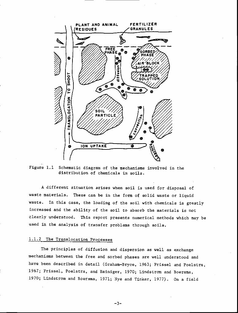
1.1 Schematic diagram of the mechanisms involved in the 3distribution of chemicals in soils.

1.2 (a) Soil water diffusivity as a function of soil water 7content. Functions shown were drawn after Gardner (1960).(b) Hydraulic conductivity as a function of soil watercontent. Functions shown were drawn after Gardner (1960).

1.3 Soil water potential as a function of soil water content. 9Functions shown were drawn after Gardner (1960).

3.1 Schematic diagram showing details of method of the "Golden 48Section Search" for locating the minimum of a function H.

3.2 Flow chart of the method of iteration used to calculate the 48plant surface potential .

ps

3.3 Flow chart of the method of iteration used to calculate the 55water content.

3.4 Conceptual diagram of the method used to determine con- 57vergence of the iterator for calculating the flux of waterat the soil surface.

3.5 Flow chart of the method of iteration used in the calcula- 65tion of the water flux at the soil surface.

LIST OF TABLES

Table Page

1.1 Types of boundary conditions for the flow equation based on 10

water content.

1.2 Types of boundary conditions for the equation describing 20

solute flow in the liquid phase.

1.3 Equilibrium models for sorption of solute onto soil 20

particles under isothermal conditions.

1.4 Non-equilibrium models for sorption of solute onto soil 21

particles under isothermal conditions.

1.5 Source/Sink models of solute. 28

2.1 Initial guesses for the water content iterator where 0 0 (z i) 33

is the value for the initial condition at the i-th node andR(0,t) is the flux specified at the soil surface at timelevel (k+1).

2.2 General form of the tri-diagonal matrix obtained by finite 33

differencing the flow equation based on water content.

2.3 The values of PICK(j). 39

2.4 The finite-difference forms of the equilibrium sorption 44

terms according to the Crank-Nicolson scheme.

2.5 The finite-difference forms of the non-equilibrium sorption 44

terms according to the Crank-Nicolson scheme.

3.1 Example of a guess-compute failure in the successive 46

averaging method.

-iv-

OR-NATURE: THE NUMERICAL ANALYSIS OF

TRANSPORT OF WATER AND SOLUTES THROUGH SOIL AND PLANTS

VOLUME I. THEORETICAL BASIS

1. THEORETICAL BASIS OF THE MODEL

1.1 Introduction

The interest of soil scientists in the development of the capability

to describe transfer processes in soils was prompted by the desire to be

able to predict accurately the behavior and movement of water, solutes,

and energy in the soil as it affects plant growth.

This interest received renewed emphasis from recent concerns about

the impact of agricultural and forestry practices on water quality. The

basic goal of forestry and agriculture is to manage the land for maximum

rate of production of fiber and food. Although this effort has been

successful, it has not been without cost or sacrifice. Management prac-

tices have resulted in increased erosion and have added to the natural

burden of nutrient elements in streams.

There are many misunderstandings about the consequences of specific

management practices on degradation of soils, groundwater, and surface

waters. These can only be resolved by a clear understanding of the

transfer processes in soils and the effect of management practices on

these transfer processes. Further interest in the prediction of transfer

processes in soil was prompted by the growing use of land for the dis-

posal of a wide variety of waste products. There is an urgent need to

predict the long-term consequences of these practices with respect to

the quality of soil and groundwater.

This report considers the transient, one-dimensional problem of

water and solute movement in the layer of soil important for plant

growth. It considers problems of infiltration of rainfall or irrigation

water, evaporation, redistribution of water in the soil, and uptake of

water by plant roots.

The distribution of ions in soils is determined by sources and

sinks, the form of the exchange isotherm, the exchange equilibria, dif-

fusion and dispersion, convection, and storage and release by plant

material. The part played by each of these factors is shown in Figure

1.1. Soil pores are assumed to be filled with water with a high concen-

tration of ions near the surface. An equilibrium exists between ions in

water (free phase) and ions retained on exchange sites of soil particles

(sorbed phase). As a result of concentration gradients in the pore

water, diffusion occurs. Some of the ions at the moving diffusion front

are removed from the free phase by adsorption onto soil particles, thus

maintaining a concentration gradient. Movement of ions as a result of

mass flow of water also occurs. It is accompanied by sorption at the

moving front and desorption at the tail. When mass flow occurs, dif-

fusion is usually less important. Ions which are not removed from the

root zone with water passing through it are available as plant food.

This sink is no longer present when vegetation is removed and the poten-

tial then exists for nutrient loss from the soil to the ground water.

1.1.1 The Sources of Ions

The ions in the soil solution are obtained from many sources. The.

natural soil system releases ions to the soil solution as a result of

the dissolving action of soil water. The rate at which ions go into

solution depends on, among other variables, the pH, the temperature of

the water and the rate of removal of the ions by the leaching process.

In a dynamic system with plants present, ions also become available from

the decaying material at the soil surface and roots below the soil

surface.

The natural system can be disturbed by activities of man. Among

the disturbances are application of fertilizers to vegetation, removal

of trees, and burning. When crops are removed, much organic material is

left at the soil surface. The disturbance with respect to the ion

balance involves, first of all, the removal of the sink. Ions removed

by plant growth are available for leaching. An ion source at the soil

surface also is added from decaying organic material.

-2-

00

0I-

0

0

1/4••••■ sON■

...saM11.9

FREE •HASE•0

Ota)

aliC1945:0002=4,

SORBEDPHASE////

‘AIR BLOCK

VIIIIT1PAP/PEDSOLUTION

O

0oc•

PLANT AND ANIMAL FERTILIZERGRANULES

0

ION UPTAKE 0

Figure 1.1 Schematic diagram of the mechanisms involved in thedistribution of chemicals in soils.

A different situation arises when soil is used for disposal of

waste materials. These can be in the form of solid waste or liquid

waste. In this case, the loading of the soil with chemicals is greatly

increased and the ability of the soil to absorb the materials is not

clearly understood. This report presents numerical methods which may be

used in the analysis of transfer problems through soils.

1.1.2 The Translocation Processes

The principles of diffusion and dispersion as well as exchange

mechanisms between the free and sorbed phases are well understood and

have been described in detail (Graham-Bryce, 1963; Frissel and Poelstra,

1967; Frissel, Poelstra, and Reiniger, 1970; Lindstrom and Boersma,

1970; Lindstrom and Boersma, 1971; Nye and Tinker, 1977). On a field

-3-

scale, the problem of ion translocation, however, is, very complex and

has not been treated in a quantitative manner. The greatest complica-

tions are brought about by continuous changes in soil water content. A

simple series of events may be recognized. In many areas, soils are at

or near freezing temperatures while a layer of snow accumulates on the

surface. In early spring, snow melts and water enters the soil to

gradually increase the water content. During this time, adsorbed ions

go into solution, diffusion to lower soil layers occurs, and ions may

become evenly distributed throughout the soil profile.

What happens as the seasons progress depends on the amount of water

available. In some geographic regions, there is just enough water to

saturate the profile without deep seepage occurring. The nutrients

remain in solution where they are available for plant growth. If more

water is available, it passes through the profile and carries ions with

it. The sequence of events described on a seasonal scale also occurs on

a shorter time base within a season as during a series of drying and

wetting periods resulting from intermittent rainfall.

Predicting ion movement in soils is clearly a complex problem.

There is extensive literature about the movement of chemicals through

soils (Nye and Tinker, 1977; Frissel, 1978). Little use has been made

of this information for quantitative predictions. This lack of practical

application of existing theory must be attributed to the problem of

applying solutions developed for idealized steady-state systems to

situations where nonisotropism is important, the boundary conditions are

ill-defined, and the processes are transient in nature.

Given these circumstances, it is not surprising that the advances

which have been made in the development of predictive capabilities have

been based on sampling techniques. In this approach, a high volume of

data is collected with the hope that upon analysis, results will show

sequences which can be correlated with certain physical and chemical

properties of the systems (Gessel and Cole, 1965; Johnson et al., 1968;

Keller, 1970).

For example, a seasonal cycle in the concentration of a certain ion

in streams may be observed which is correlated with changes in physical

properties of a watershed. The properties of the watershed can be

-4-

changed--through vegetation removal, for example--and how the previously

observed stream concentrations change can be determined.

Such a procedure has many drawbacks. It is costly and very slow.

Several years of data collection are required to calibrate the system.

Upon imposing the desired perturbations on the system many additional

years of data collection are required and, in the end, even upon establish-

ment of certain correlations, it is still difficult to assign fundamental

explanations to causal relationships.

The problem also may be approached through numerical analysis. In

this case, a mathematical model is developed which is based on a physical

description ofthe process to be studied. Analytical models differ from

statistical models. They are based on a statement of physical laws

which govern the process to be studied, and may be for steady-state or

transient conditions. This report describes a procedure for the numerical

analysis of the problem of water and chemical transport in soils.

1.2 Flow of Water

The general partial differential equation of flow of water in

soil in a vertical direction is given by Philip (1969) as

38Dt

[K(e) 14)..] ame)3z az

[L,3,7/0 /1] , (1.1)

where e is the volumetric water content [I, 3/L

3 ]; 4) is the matric potential

wof the soil water [Lp ], which is a negative quantity when the soil is

unsaturated; z is the vertical coordinate [L], positive downwards; t is

time [T]; and K(8) is the hydraulic conductivity [L 3/L

2/T]. Equation (1.1)

is usually solved as a function of water content rather than matric

potential, to reduce the effect of hysteresis in the hydraulic conductivity

function (Hillel, 1971) and to reduce the large change in the hydraulic

conductivity during infiltration of dry soils.

Equation (1.1) holds for homogeneous soils as long as the effects

of hysteresis on the function K(0) are ignored. It cannot be used to

describe conditions where deep surface ponding occurs or where a fluctu-

ating water table occurs. However, it can be used with saturated boun-

daries such as those which occur with shallow ponding or a fixed water

-5-

table. The equation will be solved using either the volumetric water

content, 6, or the water potential i as the dependent variable. Both

solutions are computed and are printed out by the computer program

OR-NATURE. A solution using the diffusivity potential obtained by the

Kirchhoff transformation will also be presented.

1.2.1 Solution Based on 6

In a homogeneous soil where K and * are single-valued functions of

e, i.e., no hysteresis, a function D may be defined such that

D = K /IQ • CNVRSN [L2 IT],

36(1.2)

where CNVRSN converts the units of potential to the units of pressure

head. The function D is called the diffusivity function. This nomen-

clature is based on its analogy to thermal diffusivity.

The transient, isothermal, one-dimensional equation based on water

content for the vertical movement of water with a root sink term can then

be written as

at . az [— qz ] + A(z,6,*ps)ae a [L3/L

3/T],

qz = - D(6) — + K(6)

3 23z

[Lw/L /T]

where *ps

the plant

water upt

or Darcia

quantity.

is the water potential [L ] in the plant at the point where

stem intersects the soil surface, A(z,6,* ) is the rate ofps

ake [L3/L

3 /T] by roots at a depth z, and q z is the volumetric

w n flux [L

3/L

2 /T]. The root uptake function A is a negativew

It is further described in Section 1.4.

There is no general analytical solution for Equation (1.3) because

the functional relationships between D and 6 and K and 6 are non-linear.

Typically, D and K vary through five to six orders of magnitude when the

soil water content ranges from wet to dry (Figure 1.2). Philip (1955,

1957) developed quasi-analytical solutions to Equation (1.3) for several

sets of special boundary conditions (Vol. III, Section 6.5). Most of

the quasi-analytical solutions use the Boltzmann similarity transform.

-6-

100

>-I-- -5: 10

3

-104

cpC) 5c.) 10

.;:x _6cr 10>-=

-107

-810 0 .10 .20 .30 .40 .50 .60

WATER CONTENT (CM3/CM3)

-3-10

WATER POTENTIAL (BARS)Figure 1.2. a. Soil water diffusivity as a

function of soil water content.Functions shown were drawn afterGardner (1960).

b. Hydraulic conductivity as a functionof soil water content. Functionsshown were drawn after Gardner (1960).

-2 1 I10 2

-10 -1010

-10-1

-10-2

-10

This technique can not be used when flux type boundary conditions are

specified. The Kirchhoff transform of the flow equation, however, can

be used and is described in Section 1.2.3. The case where A is zero has

been solved numerically by many investigators, including Hanks and

Bowers (1969), Rubin and Steinhardt (1963), and Bresler (1973).

The water content is subject to the physical constraints that

d< e(z,t) —

< es 3

/L3], (1.4)

where the subscripts d and s denote air-dry and saturated conditions.

For computational purposes, Feddes et al. (1974) determined that in the

absence of field data one may define e d as the water content which is at

equilibrium with an environment at very low relative humidity,

ed = e(IPd )

such that the potential

RTo

= M

ln(RH)1/CNVRSNwg

[L3/L

3],

[ Lp],

(1.5)

(1.6)

tant (ML2/T

2/°K/mole], T

o is the

the molecular weight of water [M/mole],

ity [L/T2 ], and RH is the relative

of the air above the soil surface, given as a ratio.

The matric potential can be obtained by using the soil-water

characteristic curve to convert from water content to water potential.

Ignoring hysteresis and assuming the soil to be homogeneous, the soil-

water characteristic curve gives a unique, one-to-one relationship

between matric potential and water content (Figure 1.3). Such a curve,

Ige), must be experimentally determined and is unique for each specific

soil.

To obtain a unique solution to Equation (1.3), the initial condi-

tion and the upper and lower boundary conditions in the soil column must

be specified.

where R is the universal gas cons

absolute temperature PK], Mw is

g is the acceleration due to gray

humidity

-8-

-102

<al -10

1

U-I 0I— -10Oa_

w

•4r -1-10

-2-10 0 .10 .20 .30 .40 .50 .60

WATER CONTENT (CM3/CM3)

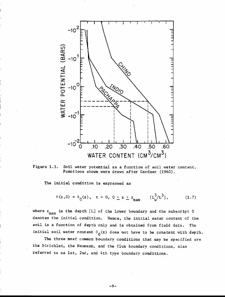
Figure 1.3. Soil water potential as a function of soil water content.Functions shown were drawn after Gardner (1960).

The initial condition is expressed as

e(z,0) = 6 0 (z), t = 0, 0 < z < zmax

[L3 /L3 ], (1.7)

where zmax is the depth [L] of the lower boundary and the subscript 0

denotes the initial condition. Hence, the initial water content of the

soil is a function of depth only and is obtained from field data. The

initial soil water content e (z) does not have to be constant with depth.0The three most common boundary conditions that may be specified are

the Dirichlet, the Neumann, and the flux boundary conditions, also

referred to as 1st, 2nd, and 4th type boundary conditions.

-9-

1st type: Dirichlet, specifies the water content, 0.

2nd type: Neumann, specifies the water content gradient, ae3z

4th type: specifies the surface flux, R = -D 22-+ K.3z

Calling the flux condition a 4th type boundary condition is arbitrary

but strictly speaking, there is no 3rd type boundary condition. A truly

3rd type boundary condition would be of the form ja0 + b(38/3z)], where

a and b are coefficients independent of 0. The 3rd type boundary condi-

tion as defined here does not occur in soil systems.

Boundary conditions must be independently specified for the upper

and lower surfaces. The upper surface is located at z = 0 and the lower

surface at z = zmax

for either vertical or horizontal coordinate orienta-

tions. Table 1.1 lists the typical types of boundary conditions that

may be encountered.

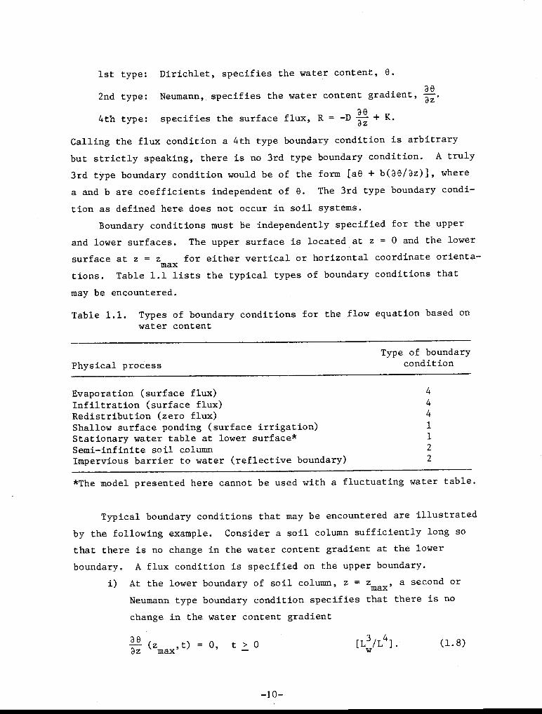
Table 1.1. Types of boundary conditions for the flow equation based onwater content

Type of boundary

Physical process condition

Evaporation (surface flux) 4

Infiltration (surface flux) 4

Redistribution (zero flux) 4

Shallow surface ponding (surface irrigation) 1

Stationary water table at lower surface* 1

Semi-infinite soil column 2

Impervious barrier to water (reflective boundary) 2

*The model presented here cannot be used with a fluctuating water table.

Typical boundary conditions that may be encountered are illustrated

by the following example. Consider a soil column sufficiently long so

that there is no change in the water content gradient at the lower

boundary. A flux condition is specified on the upper boundary.

i) At the lower boundary of soil column, z = z, a second ormax Neumann type boundary condition specifies that there is no

change in the water content gradient

113- (z t) = 0, t > 0az max'[L

3/L

4]. (1.8)

- 1 0-

ii) At the upper boundary, z = 0, a general flux condition is

specified by

De- D + K = R(0,t) 3 2

[1,w/L /T], (1.9)

where R(0,t) equals the potential surface flux, IL 3/L

2/T],

after accounting for irrigation, rainfall, and evaporation

rates. The three most common cases considered for R(0,t) are

characterized by:

R(0,t) > 0 infiltration

R(0,t) = 0 redistribution or drainage

R(0,t) < 0 evaporation [Lx3.7./L2/T]. (1.10)

Note that the flux has a positive value when the flux moves in the

positive z direction (e.g., downwards) and a negative value when the

flux moves in the negative z direction (e.g., upwards).

It should be pointed out that the "potential" flux rate, R(0,t),

for a given soil depends only on atmospheric conditions and is specified

as a function of time. The actual flux across the surface, q(0,t), is

determined by the ability of the soil to transmit water through the soil

surface. Thus, the exact flux at the soil surface cannot be predicted a

priori but is subject to the condition that its magnitude be as large as

possible, but not greater than the magnitude of the potential rate,

lq(0,01 < IR(0,t)I

[L3/L

2 IT]

and that the resulting water content profile does not violate the air-

dry and saturation limits of Equation (1.4). In general, the potential

flux, R(0,t), is specified and the computer program solves for the

actual surface flux, q(0,t), subject to Equations (1.4) and (1.11) by

iteration. Additional details are given in Section 3.4.

1.2.2 Solution Based on 1p

The flow equation for transient, isothermal, one-dimensional condi-

tions with flow in the vertical direction can be written in terms of

matric potential as

at (3 )

=

3z3z [K CNVRSN - K] + A(z,1),4ips)

4) (1.12)

3 3[Lw/L /T],

where (38/30 is the "specific water capacity," i.e., the slope of the

soil-water characteristic curve. All other terms were defined earlier.

Equations (1.3) and (1.12) are numerically identical, even though the

notation is different. The soil-water characteristic function, 060,

is needed to evaluate the specific water capacity term and to convert

matric potential to volumetric water content. Thus, when Equation (1.12)

is solved numerically, the computer program converts the potential to

water content when evaluating K(0).

The solution of Equation (1.12), the potential-based flow equation,

is subject to the limits on water content at air-dry and saturated

conditions, initial conditions, and boundary conditions. The range of

matric potentials is bounded by the potentials for air-dry and saturated

soils

< ip(z,t) < *a (Lp]. (1.13)

In general, saturation is defined by

= 0

(1.14)

Matric potential is defined as a negative quantity when the soil is

unsaturated and a positive or zero quantity when the soil is saturated.

The flow equation based on matric potential (Equation 1.12) is valid

only for unconfined, unsaturated (II) < 0) soil conditions. However,

Equation (1.12) can be used when the soil is saturated at the boundary

> 0). Thus, either surface ponding or a stationary water table can be

specified at the boundaries.

The initial condition is:

ip(z,0) = ip 0 (z) at t = 0, 0 < z < z a ], (1.15)m x p

where subscript 0 denotes the initial condition.

-12-

F(p) = CNVRSN er KW)dip' [L3 /L/T], (1.17)

4)►:21Pd

The boundary conditions for the upper and lower boundaries are

identical to those of the equations based on water content with appro-

priate changes in notation. The three types of boundary conditions are

defined as

1st type: specified potential, IP,

2nd type: specified gradient, az'4th type: specified surface flux, R = - K

az CNVRSN + K.

1.2.3 Solution Based on Diffusivity Potential (Kirchhoff Transform)

Numerous investigators, including Remson et al. (1971), Bear (1972),

and Braester (1972), introduce a new variable, called the diffusivity

potential, F. A variable of this type is usually referred to as a

Kirchhoff transform variable and is defined as either

F(8) =fe,=e D(e')dei [L3 /L/T], (1.16)

or as

where D(0) is the soil water diffusivity and K(8) is the hydraulic con-

ductivity. For a given soil-water characteristic curve, 19 and IP are

uniquely related, hence

F(e) = F(4))

L3 /L/TJ. (1.18)

Braester (1972) gives several tables of F for different soils. The

lower limit of F is defined as

F(C1d) = 0 [L 3 /L/T], (1.19)

F(tpd ) = 0 [L134/L/T]. (1.20)

F is always defined as a positive quantity which monotonically increases

in value when going from air-dry to saturated conditions.

-13-

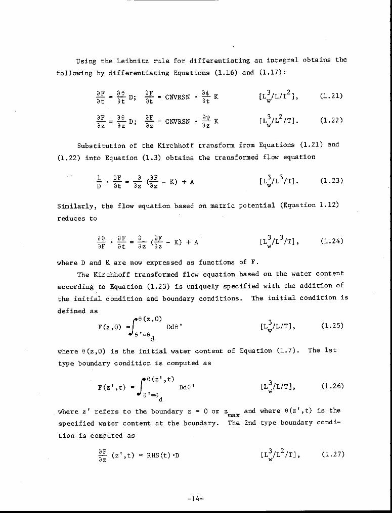
Using the Leibnitz rule for differentiating an integral obtains the

following by differentiating Equations (1.16) and (1.17):

9F ae aF= D.

CNVRSN • 21- K [L3/L/T

2 ], (1.21)Bt at' 3t = at

aF ae aF= 7 -D; = CNVRSN • az K [L

3 /L2 /T]. (1.22)

az

Substitution of the Kirchhoff transform from Equations (1.21) and

(1.22) into Equation (1.3) obtains the transformed flow equation

. DF _ a (aFD 3t 3z ‘az

)

A 3 3[Lw/L /T]. (1.23)

Similarly, the flow equation based on matric potential (Equation 1.12)

reduces to

ae aF a ( DI',) A

BF at — 3z

( a [L3 /L

3/T], (1.24)

where D and K are now expressed as functions of F.

The Kirchhoff transformed flow equation based on the water content

according to Equation (1.23) is uniquely specified with the addition of

the initial condition and boundary conditions. The initial condition is

defined as'e (z,0)

=4,F(z,0) 1 Dde'e'=e

d

[L3w/L/T], (1.25)

where e(z,0) is the initial water content of Equation (1.7). The 1st

type boundary condition is computed as

e(z',0

F(z',t) = J Dde' [L 3 /L/T],e'=e

d

where z' refers to the boundary z = 0 or z and where e(z I ,t) is themax

specified water content at the boundary. The 2nd type boundary condi-

tion is computed as

DFaz

(z ,t) = RHS(t)-D [L3 /L2 /T], (1.27)

(1.26)

- 14L

aewhere RHS(t) = (z',t) is a specified function of time on the boundary

(e.g., Equation (1.8)) and where D is the soil water diffusivity evalu-ated at the boundary. The 4th type boundary condition is computed as

3F- — + K = RHS(t)Dz3 2[Lw/L /T], (1.28)

where RHS(t) = (- D 2±-+ K) is a specified surface flux (e.g., Equation3z(1.9)).

The range of the transform variable is

Fd < F(z,t) < F

s [L134/L/T], (1.29)

where F s = F(e s ) and Fd = F(ed).The Kirchhoff transformed flow equation can also be expressed in

terms of matric potential, such as in Equation (1.24). Then the initialcondition is

11)(z,0)F(z,0) =4,1.Kdtpl-CNVRSN

IP'=4)d[L 3 /L/T], (1.30)

where tp(z,0) is the initial matric potential of Equation (1.15). The1st type boundary condition, at z = 0 or z = z ismax

tp(z1,t)F(z',t) Kdipt•CNVRSN [L 3/L/T],

4)'=4'dwhere 11)(z y ,t) is the specified matric potential at the boundary. The2nd type boundary condition is

DFaz (z ,t) = RHS(t)•K•CNVRSN 3 2

[Lw/L /T], (1.32)

where RHS(t) = 9z

(z'' 0 is a specified function of time on the boundary

and where K is the conductivity evaluated at the boundary. The 4th typeboundary condition is

–K = RHS(t) [L 3 /L2 /T], (1.33)Dz

where RHS(t) = (- K t • CNVRSN + K) is a specified surface flux. Therange of the transform variable is the same as in Equation (1.29).

(1.31)

-15-

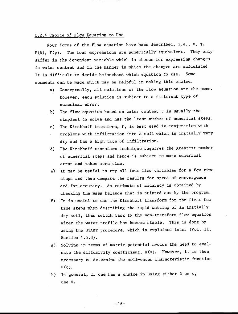
1.2.4 Choice of Flow Equation to Use

Four forms of the flow equation have been described, i.e., e,F(e), F(4)). The four expressions are numerically equivalent. They onlydiffer in the dependent variable which is chosen for expressing changes

in water content and in the manner in which the changes are calculated.

It is difficult to decide beforehand which equation to use. Some

comments can be made which may be helpful in making this choice.

a) Conceptually, all solutions of the flow equation are the same.

However, each solution is subject to a different type of

numerical error.

The flow equation based on water content e is usually the

simplest to solve and has the least number of numerical steps.

c) The Kirchhoff transform, F, is best used in conjunction with

problems with infiltration into a soil which is initially very

dry and has a high rate of infiltration.

d) The Kirchhoff transform technique requires the greatest number

of numerical steps and hence is subject to more numerical

error and takes more time.

e) It may be useful to try all four flow variables for a few time

steps and then compare the results for speed of convergence

and for accuracy. An estimate of accuracy is obtained by

checking the mass balance that is printed out by the program.

f) It is useful to use the Kirchhoff transform for the first few

time steps when describing the rapid wetting of an initially

dry soil, then switch back to the non-transform flow equation

after the water profile has become stable. This is done by

using the START procedure, which is explained later (Vol. II,

Section 4.5.3).

g) Solving in terms of matric potential avoids the need to eval-

uate the diffusivity coefficient, D(6). However, it is then

necessary to determine the soil-water characteristic function

e(0.

h) In general, if one has a choice in using either e or

use 0.

-16-

1.3 Solute Displacement Equation

The displacement of solute by mass flow of water is described by

Dutt et al. (1972) and Bresler (1973) as follows:

l a ac asz at - (v)la{ec}az sz

afqclai

az + G(z,t,e,c,S)

IM/L3/T],

(1.34)

where c is the solute concentration in solution (liquid phase) [M/L 3],

S is the local solute concentration in the sorbed or solid phase [Ma3 ],

D is the apparent solute dispersion coefficient [L2/T], G is thesz

solute source/sink term [M/L 3/T], q is the volumetric or Darcian flux

z[L3 /L2 /T], v is the magnitude of the pore-water velocity, v = lq

z/ 01

[L/T], and t is the time [T].

The first term on the right-hand side of Equation (1.34) describes

the solute flux caused by diffusion and by hydrodynamic dispersion

processes. The apparent solute dispersion coefficient, D, includessz

the effect of hydrodynamic dispersion and molecular diffusion. The

second term in Equation (1.34) represents the solute flux from mass

transport processes.

The equation as stated allows diffusion to occur when the mass flow

rate of water or the convection term is zero. It also includes an

expression for the sorption or desorption of the solute onto soil

particles and a solute source or sink term. The source/sink term can

describe the addition of solute to the soil in the form of fertilizers,

slow decay of organic matter, addition of hazardous chemicals, slow

leaks from storage tanks for hazardous chemicals, and solute uptake by

roots.

1.3.1 Solute in the Liquid Phase

To obtain a unique solution to Equation (1.34), initial conditions

and boundary conditions on the upper and lower soil surfaces must be

specified. The initial concentration of the liquid phase is

c(z,0) = c0(z)

[M/L3 ]. (1.35)

-17-

There are three common types of boundary conditions that can be

specified for the liquid phase solute. These are the Dirichlet, Neu-

mann, and the Cauchy types.

1st type: Dirichlet, specifies surface concentration, c.

2nd type: Neumann, specifies the concentration gradient, ac

3rd type: Cauchy, specifies solute flux through the soil

surface, f = qzc - 8 D (9c/az).

sz

Table 1.2 lists the more common types of boundary conditions that may be

encountered. Details about third type boundary conditions are given by

Bresler (1973). If we define f(t) as the liquid phase solute flux

through the soil surface with z = 0 at the upper surface

f(t)Iz=0

- = {- 6•Dac— + q c}I + [M/L2 /T], (1.36)

sz az z z=0

then

for infiltration f(t) = qz(0,t)c(0,t),

for redistribution f(t) = 0, q z (0,t) = 0,

for evaporation f(t) = 0, qz (0,t) < 0, [M/L2 /T], (1.37)

where superscript (-) indicates above the boundary and superscript (+)

indicates below the boundary. The solute flux, f(t), that moves in the

positive z direction (e.g., downward) is computed as a positive flux and

a flux that moves in the negative z direction (e.g., upwards) is com-

puted as a negative flux. Usually a zero gradient condition can be

assumed for the lower surface

(z = 0 [M/L3/LI (1.38)

az max'

However, Equation (1.38) cannot be used to describe movement in a short

soil column where the solute reaches the end of the soil column.

1.3.2 Solute in the Solid Phase

To solve Equation (1.34), the sorption term, S, must be described

mathematically. Many different models for sorption have been proposed.

Boast (1973) and van Genuchten and Cleary (1979) give a detailed review of

-18-

these. In choosing any one of the models, the limitations imposed on

their derivations should be recognized. All the models imply a homoge-

neous sorbing medium in the sense that the activation energy of the

sorbing reaction is invariant within the medium, i.e., the soil is

comprised of only one mineral.

Another serious limitation of most models is the fact that the

analyses are based on a steady-state, saturated flow. The application

of such models to a real soil and unsaturated conditions may be limited

by this. Certain discrepancies between results obtained with these

models and experiments are expected. The equilibrium or kinetic reac-

tion constants may vary with local changes in water content. Reaction

rates differ between wet and dry soils. Assuming a homogeneous soil and

a steady-state condition, Lindstrom et al. (1970, 1971) and Lindstrom

and Boersma (1970) put forth a kinetic model (Table 1.3) which appropriately

accounts for forward and backward activation energies. The model can be

applied to both adsorption and desorption. When van Genuchten et al.

(1974) extended the model to a saturated soil column,'they found that

the model was inadequate to handle the non-homogeneity of the medium.

In particular, the model does not incorporate the effect of residence

time of chemical in the sorption process which results in greater devia-

tion from the experimental values at higher pore-water velocities.

Clearly, more study is needed to obtain a realistic sorption model which

will satisfactorily circumvent the complexity of the soil (Yingjajaval,

1979).

Listed in Table 1.3 are some of the sorption models for equilibrium

reactions which have been incorporated in the computer program. Non-

equilibrium models are given in Table 1.4. The equilibrium models are

special cases of the non-equilibrium models, with 8S/8t having been set

to zero.

The user must use his judgment in selecting one of these models.

He should choose one which he thinks is most appropriate to his experi-

mental conditions. The models shown in Tables 1.3 and 1.4 assume that

sorption and desorption are defined by the same equation. Additional

details of the use of these models are in Sections 2.2 and 3.6.

-19-

Table 1.2. Types of boundary conditions for the equation describingsolute flow in the liquid phase

Type of boundaryPhysical process condition

Solute flux during water evaporation 3Solute flux during water redistribution 3Solute flux during water infiltration 3Specified solute concentration 1Impervious barrier to solute (reflective boundary) 2Semi-infinite soil column 2

Table 1.3. Equilibrium models for sorption of solute onto soil particlesunder isothermal conditions. k1 , k2, k3

and k4 are specified

constants for each model

Name Sorption model Reference

Linear S = klc + k

2

k1cLangmuir S =

(l+kc) + k

32

k2Freundlich S = k

lc + k3

Lapidus and Amundson(1952)

Tanji (1970)

Lindstrom and Boersma(1970)

Generalnon-linear

such as:

S = F(S, c)

k1cS = Lai and Jurinak (1971)

c+(k2-c)exp[k3-k4c]

-20-

at (l+k2c) + k

3S + k

4DS

kic

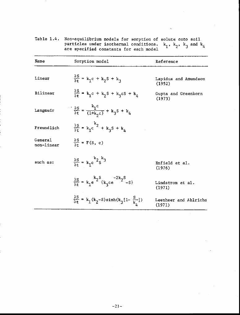
Table 1.4. Non-equilibrium models for sorption of solute onto soilparticles under isothermal conditions. k1 , k2, k

3 and k

4are specified constants for each model

Name Sorption model Reference

DS9t = kic + k2 S + k3Lapidus and Amundson(1952)

asat

kic + k2 S + k3cS + k

4

k2DS

= kic + k3S + k4

DS= F(S, c)

at

Linear

Bilinear

Langmuir

Freundlich

Generalnon-linear

Gupta and Greenkorn(1973)

such as: DS k2 k3=kcS

at 1

k2S -2k2S

atDS

= k1e {k3ce -sl

Enfield et al.(1976)

Lindstrom et al.(1971)

DS = ki (k2-S)sinh(k3 [1- IT]) Leenheer and Ahlrichs4 (1971)

-21-

Experimentally, it may be more convenient to define the sorption

term in units of mass of chemical per soil mass, s, rather than in units

of mass of chemical per unit volume as indicated by S. S can be related

to s by

S = s • BD [M/L3] (1.39)

where BD is the bulk density of the soil [Asoil

/L3 ] and s is the sorp-

tion on a mass basis [M/Msoil].

The computer program does not use Equation (1.39) and the above is

only given for general interest. The program assumes the sorption term,

S, to have units of [M/L3].

1.4 Water Uptake by the Roots

Leaves evaporate water in response to the evaporative demand of the

atmosphere. The rate corresponding to the evaporative demand of the

atmosphere is called the potential transpiration, q . The water lostpsby the leaves is replaced by water adsorbed by the roots from the soil

and transferred along the plant stem. When the rate of water supply

from the roots to the leaves does not equal the evaporative demand, the

potential of the water in the leaf cells decreases, which results in

stomatal closure. The model used in this report is based on a "plant

surface potential", * , which is the potential of the water in theps

plant stem at the soil surface. Some authors call this the root-collar

potential. Other authors (Gardner, 1964; Whisler et al., 1968; Molz and

Remson, 1971; Nimah and Hanks, 1973; Neuman et al., 1975; Taylor and

Klepper, 1975; Farnum, 1977; Molz, 1981) have used similar models.

Several modifications have been used in the analysis presented here.

The root uptake model, developed by Ungs et al. (1977), is given as

{[* -*] • CNVRSN + z + RPF}pA =

s • RAY [L3 /L3 /T].

1 1 •w1-.k + k 1

r

(1.40)

This model is based on the following concepts:

-22-

a) The actual rate of transpiration, T r , is some fraction of the

potential evaporative demand, q of the atmosphere. This fraction isps

determined by the stomatal correction factor, c, which is a knownst

function of the plant water potential at the soil surface. Then the

actual transpiration rate is described by

Tr = cips(t).est(4)ps)

The potential evaporative demand depends only on climatic conditions and

is given as a function of time.

b) The plant surface potential, * , is not a priori known andps

changes at each time step in response to the potential demand and soil

supply conditions. A value of t is "hunted" for until the totalps

amount of water extracted by the plant roots over the soil column

occupied by roots equals the actual transpiration rate, T r . The plant

surface potential * is bounded by the condition thatps

*wilt —< p < 0, [L , (1.42)

where *wilt is the water potential at which the plant permanently wilts

and dies.

c) The water potential of the root, * r , is equal to the sum of the

plant surface potential, the distance from the soil surface to the root

(gravity potential), and RPF, which is a specified function describing

the friction loss incurred by the water flowing through the root xylem

to the soil surface

*r(z,e,* ps ) = * ps + {z+RPF}/CNVRSN

[Lp]. (1.43)

d) The flow of water from the soil to the root is proportional to

the difference between the soil matric potential, *, and the potential

of the root

(1P r- [L ], (1.44)

where *, corresponding to a given value of 0, is computed from Equation

(1.12) or from the soil-water characteristic function.

e) The hydraulic conductivity through the soil-root system,

K (8) [L3 /L2 /T], is proportional to the conductivities of the soilsys

[L3w/L

2/T]. (1.41)

-23-

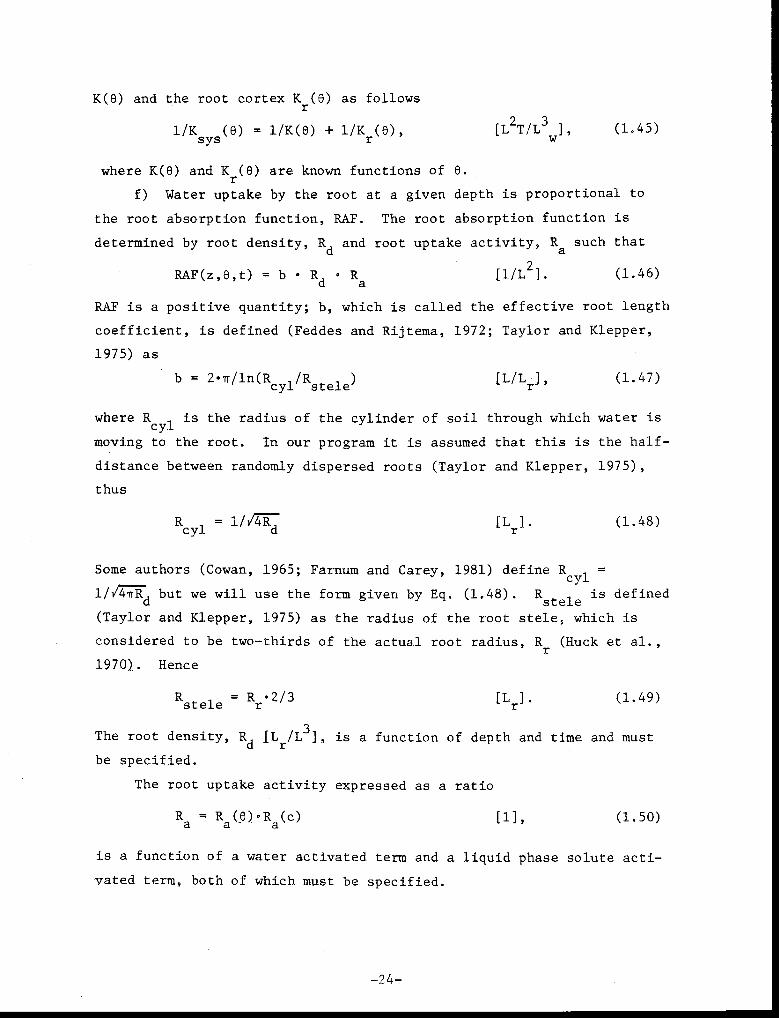
K(6) and the root cortex Kr(6) as follows

1/K (e) = 1/K(6) + 1/Kr(6),sys

[L2T/L

3w], (1.45)

where K(6) and Kr(6) are known functions of 6.

f) Water uptake by the root at a given depth is proportional to

the root absorption function, RAF. The root absorption function is

determined by root density, Rd and root uptake activity, R

a such that

RAF(z,6,t) = b • Rd • Ra [1/L 2 ]. (1.46)

RAF is a positive quantity; b, which is called the effective root length

coefficient, is defined (Feddes and Rijtema, 1972; Taylor and Klepper,

1975) as

= 2 • 1-/ln(Rcy_/R [L/Lr], (1.47)i stele)

where Rcl

is the radius of the cylinder of soil through which water isY

moving to the root. In our program it is assumed that this is the half-

distance between randomly dispersed roots (Taylor and Klepper, 1975),

thus

Rcyl

= 1//717 [Lr]. (1.48)

Some authors (Cowan, 1965; Farnum and Carey, 1981) define Rcyl

1/47R- but we will use the form given by Eq. (1.48). Rstele

is defined

(Taylor and Klepper, 1975) as the radius of the root stele, which is

considered to be two-thirds of the actual root radius, Rr (Huck et al.,

1970). Hence

Rstele

= Rr•2/3 [Lr]. (1.49)

The root density, Rd IL

r/L

3], is a function of depth and time and must

be specified.

The root uptake activity expressed as a ratio

R = R (e).R (c) [1], (1.50)a a a

is a function of a water activated term and a liquid phase solute acti-

vated term, both of which must be specified.

-24-

g) The flux of water withdrawn from each soil layer by the roots

in that layer is defined by the root uptake term, A, where

A(z,0,ps ) = K

sys. RAF . {ip r- tp} . CNVRSN [I,

3/L

3/T] (1.51)

and upon substitution of Equation (1.43), the root uptake at the i-th

soil layer is

Ai K . RAF . {(4) - 11) • CNVRSN + z + RPF}3w/L3 /T].1 sys ps (1.52)

However, if Ai > 0, set Ai = 0.

h) The actual transpiration rate, T, from step a) must equal ther

sum of the amounts of water withdrawn from all soil layer sinks

n-1(zi+1

- zi-1

)A.

23 2

[Lw/L /T]. (1.53)

i=2

The sum is from i = 2,...,n-1 since it is assumed there is no uptake of

water by roots at the top and bottom nodes.

To determine the actual transpiration rate, T r , the computer program

uses an iterative scheme:

Step i) Specify the potential transpiration demand, q, and guessps

the soil matric potential for each soil layer.

Step ii) Guess the plant surface potential, f, subject to theps

conditions of Equation (1.42).

Step iii) Compute the actual transpiration rate, Tr, using the

guessed value of ip and Equation (1.41).psStep iv) Compute the root uptake term A. for each soil layer from

Equation (1.52).

Step v) Compute the actual transpiration rate, Tr, using Equation

(1.53).

Step vi) If the transpiration rate of step iii) does not equal the

transpiration rate of step v), then make a new guess of

the plant surface potential tp and return to step ii).ps

The iterative process stops when step vi) converges. The results

of this iterative process (Section 3.2) depend on the initially guessed

values of soil matric potential, An additional iterative process is

-25-

required in which the correct soil matric potential, subject to Equa-

tions (1.12) and (1.13), is determined.

In actual practice, the iteration scheme for computing 1p convergesps

within three to five iterations. The matric potential iterator scheme,

however, may take 5 to 10 iteration cycles to compute 4). Additional

details are given in later sections.

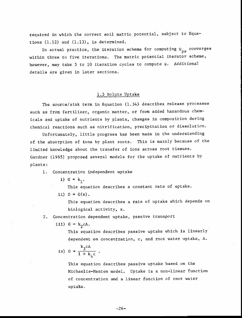
1.5 Solute Uptake

The source/sink term in Equation (1.34) describes release processes

such as from fertilizer, organic matter, or from added hazardous chem-

icals and uptake of nutrients by plants, changes in composition during

chemical reactions such as nitrification, precipitation or dissolution.

Unfortunately, little progress has been made in the understanding

of the absorption of ions by plant roots. This is mainly because of the

limited knowledge about the transfer of ions across root tissues.

Gardner (1965) proposed several models for the uptake of nutrients by

plants:

1. Concentration independent uptake

i) G = kl.

This equation describes a constant rate of uptake.

ii) G = G(x).

This equation describes a rate of uptake which depends on

biological activity, x.

2. Concentration dependent uptake, passive transport

iii) G = k2cA.

This equation describes passive uptake which is linearly

dependent on concentration, c, and root water uptake, A.

k3cA

This equation describes passive uptake based on the

Michaelis-Menten model. Uptake is a non-linear function

of concentration and a linear function of root water

uptake.

iv) G -1 + k

4c °

-26-

3. Concentration dependent uptake, active transport

v) G= k5c.

For root systems, this equation describes root solute

uptake as a function of solute concentration. Solute

transport into the root is independent of root water

uptake. This implies an active membrane transport

mechanism.

For non-root systems, this equation implies a decay/

addition of solute that is linearly proportional to the

solute concentration in the soil (Vol. IV, Section 7.5,

for example).

k6c

vi) G =

This equation describes root solute uptake as a Michaelis-

Menten model. However, unlike iv), the uptake can be a

non-linear function of both concentration and root water

uptake. Hence, k6=k6 (A), and k7=k7(A).

A more detailed discussion of the above models, including the effect of

soil temperature on root solute uptake, is given by Ungs et al. (1982).

In subroutine SOLUTE, the solute source/sink term is evaluated at

the i-th spatial node, at time level (k + 1/2) and is written as

Passive: G(i) = GCOEF • A(i) [M/L3/7], (1.54a)

Active: G(i) = GCOEF [M/L3/T], (1.54b)

where A(i) is the rate of water uptake by the roots [L 3/L

3 /T] at node iw

and time level (k + 1/2) and GCOEF is the source/sink coefficient ofWsolute 'V, [M/L

3/T] at node i. Table 1.5 lists the form of coeffi-

cient GCOEF for some of the models given above. Variable G(i) is a

negative quantity for sink models (root uptake, solute decay, and

positive for source models (solute release). Variable A(i) is always

negative for root uptake.

l+k7c

-27-

Table 1.5. Source/Sink models of solute

Name Source/Sink model

Constant

Linear

Michaelis-Menten

GCOEF = k1

GCOEF = k2*c

ik+1/2

* k+1/2k3

GCOEF =ci * k+1/2

(l+k4 c i)

where *ck+1/2 is defined in Equation (3.31)

The total amount of solute taken up by the source/sink system at

any instant is given by the sum of the amounts of solute added or

withdrawn from all soil layers

T =cr

(z. z )141 i-1 G.

2[M/L2 /T]. (1.55)

i=2

The sum is from i = 2,...,n-1 since it is assumed that there is no

source/sink at the top and bottom nodes. Also note that G i is evaluated

at (i,k + 1/2), i.e., the half-time step level.

-28-

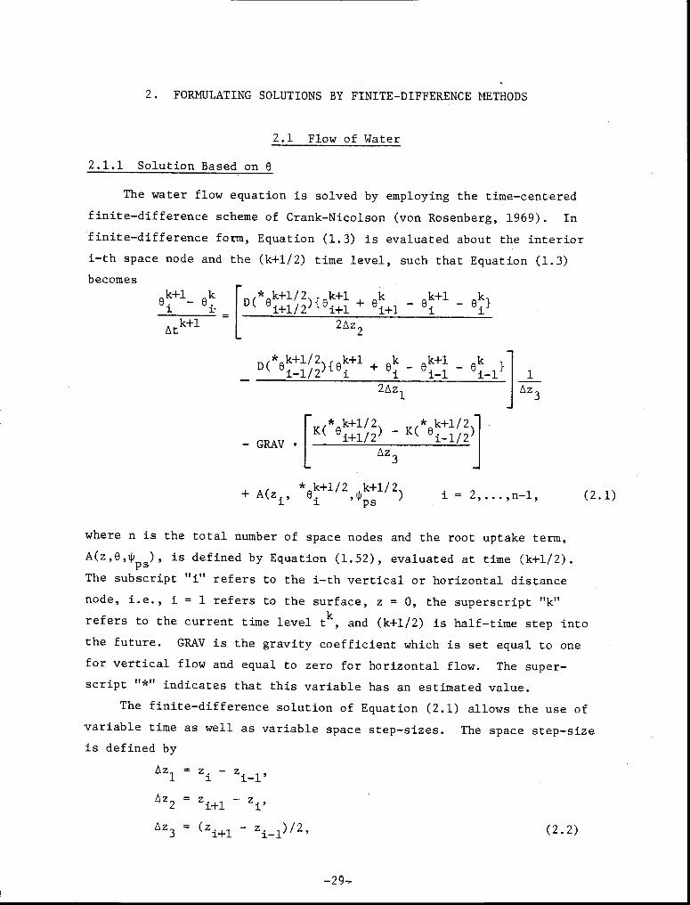
2. FORMULATING SOLUTIONS BY FINITE-DIFFERENCE METHODS

2.1 Flow of Water

2.1.1 Solution Based on 6

The water flow equation is solved by employing the time-centered

finite-difference scheme of Crank-Nicolson (von Rosenberg, 1969). In

finite-difference form, Equation (1.3) is evaluated about the interior

i-th space node and the (k+1/2) time level, such that Equation (1.3)

becomesek+1_ ekD f * ek+1/2\fek+1 ek ek+1 ek}

-i+1/21L 1+1 1+1

Atk+1 2iz2

* k+1/2 k+1 k k+1 k

1111•001-1/2 )ie

i+ e -1 e -el

i-1 i-1 1

2Az1 Az3

- GRAV •

+ A(z i ,

K( e1/

2) - K(

(2.1)i = 2,...,n-1,* 6

Az3

+1/2 k+1/2,e i oPps )

where n is the total number of space nodes and the root uptake term,

A(z,6,* ), is defined by Equation (1.52), evaluated at time (k+1/2).ps

The subscript "i" refers to the i-th vertical or horizontal distance

node, i.e., i = 1 refers to the surface, z = 0, the superscript "k"

refers to the current time level t k , and (k+1/2) is half-time step into

the future. GRAV is the gravity coefficient which is set equal to one

for vertical flow and equal to zero for horizontal flow. The super-

script "*" indicates that this variable has an estimated value.

The finite-difference solution of Equation (2.1) allows the use of

variable time as well as variable space step-sizes. The space step-size

is defined by

Az i = z i - zi-1,

k+1/2 * k+1/2

/z 2 = z1+1

- z

Az = (z - z )/23 i+1 i-1 ' (2.2)

and the time step-size is defined by

k k k-1At = t - t ,

Atk+1k+1

= t - t .

The half-time step can be related to the full-time step by

* k+1/2 * k+1 * k+1 k ki+1

+ e )/4'e i+1/2

* k+1/2 * k+1 k

* k+1/2* k+1 * k+1 k k8 = ( 8. + i-1

+ e i + i-1 )/4.i-1/2

(2.3)

(2.4a)

(2.4b)

(2.4c)

There is a total of n space nodes but Equation (2.1) is evaluated

only at the interior nodes of the soil column, from i=2,...,n-1 at time

level (k+1/2). The boundary conditions are evaluated at the first and

last node at time level (k+1) and are evaluated by a backward-difference

scheme. Hence the n-2 interior flow equations of Equation (2.1) and the

upper and lower boundary expressions comprise a total of n equations and

n unknowns for time level (k+1).

The initial condition of Equation (1.7) is expressed as

=08 i= 80 (z i) i = 1,...,n. (2.5)

Three types of boundary conditions for the upper soil surface are

allowed, namely the Dirichlet (1st type), the Neumann (2nd type), and

the 4th type involving a surface flux. These are backward-differenced

as

1st type:

k+1 = RHS(t

k+1),

2nd type:

k+1 k+18 2 - el

1 = RHS(tk+1 ),

z - zl

(2.6a)

(2.6b)

-30-

4th type:

k+1 ke l el * k+1= D(

1+1/2At

k+1

k+1 k+1 * k+12 - e K( 1+1/2 )

• • GRAV(z 2-zi )

2(z2-z1)

k+1q0 (z2-z1)

(2.6c)

In the above equations RHS(tk+1) corresponds to the specified value of

the boundary condition at time tk+1. The term q

k+1 is the actual sur-

face flux as defined by Equation (1.11), evaluated at node 1/2 (which

lies above the soil surface, z=0) and time level (k+1). In addition,* k+10 1+1/2 is defined as

* ek+1* k+1 * k+1= ( + 02 )/2.1+1/2 1 (2.7)

There are also three types of boundary conditions for the lower

soil surface. These are backward-differenced as

1st type:

ek+1 = RHS(tk+1

),

2nd type:

e k+1-

k+1n n-1

1 = RHS(tk+1),z - z

n n-1

4th type:

(2.8a)

(2.8b)

k+1 ken - en

k+1 k+1 * k+1{0n - en-1 } K( en-1/2 )*

-D( en-k+1

1/2 ) • z z) • GRAV

(n- n-1

) 2 (zn- z

n-1Atk+1

where qk+1n

lies below

addition,

k+1qn

(z- z-1

) 'n n

is the actual surface flux, evaluated at node n+1/2 (which

the lower soil surface, z=z

) and time level (k+1). Inmax*ek+1

is defined asn-1/2

(2.8c)

-31-

*8n+1/2 * k+1 * k1en-1/2 = ( en +

/2 . (2.9)en-+1)

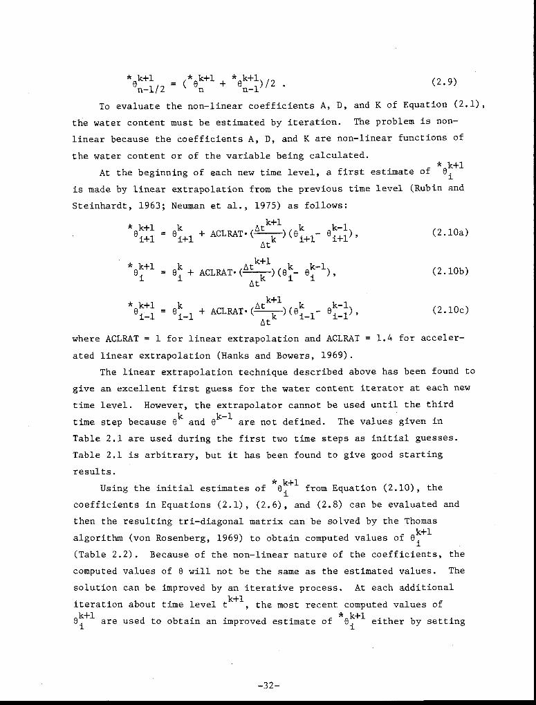
To evaluate the non-linear coefficients A, D, and K of Equation (2.1),

the water content must be estimated by iteration. The problem is non-

linear because the coefficients A, D, and K are non-linear functions of

the water content or of the variable being calculated.*

At the beginning of each new time level, a first estimate of e.k+1

is made by linear extrapolation from the previous time level (Rubin and

Steinhardt, 1963; Neuman et al., 1975) as follows:

* k+1 k k-1e i+i = 0 1.4.1 + ACLRAT-(

Atk+1 k )(0 1_1_1- ei+i),At

*8i+1 k

8 = 8 i + ACLRAT . (

Atk+1)(ek- ek-1,

Atk i

k+1

k+1 k k-*1e = 8. + ACLRAT•0

Atk i-1 1-1)(ek - e. ),

i-1 1-1

where ACLRAT = 1 for linear extrapolation and ACLRAT = 1.4 for acceler-

ated linear extrapolation (Hanks and Bowers, 1969).

The linear extrapolation technique described above has been found to

give an excellent first guess for the water content iterator at each new

time level. However, the extrapolator cannot be used until the third

time step because 8 k and ek-1 are not defined. The values given in

Table 2.1 are used during the first two time steps as initial guesses.

Table 2.1 is arbitrary, but it has been found to give good starting

results.*

Using the initial estimates of e ik+1

from Equation (2.10), the

coefficients in Equations (2.1), (2.6), and (2.8) can be evaluated and

then the resulting tri-diagonal matrix can be solved by the Thomas

algorithm (von Rosenberg, 1969) to obtain computed values of ek+1i

(Table 2.2). Because of the non-linear nature of the coefficients, the

computed values of e will not be the same as the estimated values. The

solution can be improved by an iterative process. At each additional

iteration about time level tk+1

, the most recent computed values ofk+1 * k+1ei are used to obtain an improved estimate of e i either by setting

(2.10a)

(2.10b)

(2.10c)

-32-

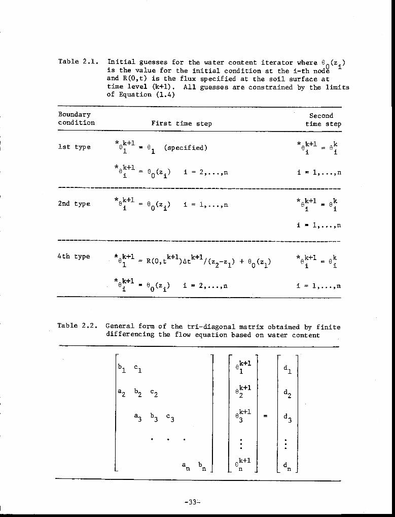
Table 2.1. Initial guesses for the water content iterator where e (z.)is the value for the initial condition at the i-th nodeand R(0,t) is the flux specified at the soil surface attime level (K+1). All guesses are constrained by the limitsof Equation (1.4)

Boundary Secondcondition First time step time step

1st type *k+1 = e (specified) e.

k+1 = B.1 1

* 1

* k+10 = 0

0(z) i = 2,...,n = 1,...,n

2nd type * k+1 * k+1 k0.=00 (z i) i = 1,...,n 8. = 8.

i = 1,...,n

4th type *ek+1

= ek*0k+1

= R(0,t k+1)Atk+1

/(z2-z

1) + 0

0 (z1 )1

*8k+1 = 8 (z ) = 2,...,n0 i i = 1,...,n

Table 2.2. General form of the tri-diagonal matrix obtained by finitedifferencing the flow equation based on water content

k+1b1 c

1 1

k+1

d1

a2 b2 c2 e2

k+1

d2

a3

b3

c3 3

d3

an bn

k+1en dn

* Knew

0

* k+1 k+18.estimat={0.01destimat0+6.(compted)}/2. (2.11)

according to Neuman et al. (1975) or by using a Newton-Raphson scheme

(Section 3.3) in the fourth and/or subsequent iteration. The iterative

procedure continues until a satisfactory degree of convergence is

obtained, usually within 10 cycles, depending on the accuracy required.

The criterion for convergence is

* k+1 k+18. - 8.

1 *8k+1max i0

WRATIO i = 1,...,n, (2.12)

where WRATIO is the maximum allowed difference, expressed as a ratio.

Some authors (Rubin and Steinhardt, 1963) have assumed that the

guess obtained by linear extrapolation of Equation (2.10) is suffi-

ciently accurate so that no iteration is attempted. Others solve the

non-linear coefficients at the old time level, tk, thereby reducing the

finite-difference equation of the water flow equation to a linear one.

In general, small time steps are necessary when a non-iterative tech-

nique is used. How small these time steps should be is a difficult

question to answer. Convergence criteria and failure to converge

problems for the iterative schemes presented in this report are further

discussed in Volume III.

2.1.2 Size of Time Step

Usually the choice of size of the time step is one of convenience.

Both the centered Crank-Nicolson and the backward-difference schemes are

unconditionally stable for all ratios of Lz and .t (von Rosenberg,

1969). However, mass balance and numerical oscillation problems can

occur if the size of the time step chosen is too large. Furthermore,

the water content iterator becomes very inefficient when large time

steps are used since the rate of convergence decreases dramatically and,

in fact, failure to converge may occur.

Program OR-NATURE provides four methods to determine the size of

the time step in subroutine STEP.

-34-

i) use the method of Hanks and Bowers, by setting the parameter

K1DELT = 0.

ii) use a general formula, by setting K1DELT = 1, with

Atk41 = a + bLtk + ctk . (2.13a)

iii) use a user specified empirical formula, by setting K1DELT = 2.

iv) fix the minimum and maximum step size such that

At=Atinin...Atmax

.

The method of Hanks and Bowers defines the step size as the length

of time required for the water to move in the soil from one node to the

next at the maximum flux rate. Hanks and Bowers (1969) and Dutt et al.

(1972) define

ek-1/2 ( - z )Atk+1

< min i+1/2z i+1 i

i = 1,...,n-1, (2.13b)k-1/2qi

k-1/+1/2zwhere the Darcian flux qi+1/2 is defined at the previous time level as

k-1/2- k-1/2

. )k-1/2 ,,,k-1/2\ i+1 1 k-1/2+ GRANT.K(19 i+1/2 ).q =i+1/2 -"i+1/21.

0

(z. - 8z.)1+1 1(2.13c)

The size of the time step according to Equation (2.13b) is constrained

to lie between the specified minimum and maximum step size limits

At < Atk+1 <_Atmax

.min — (2.14)

If the computed time step-size violates Equation (2.14), it is set to

the limiting value of either Atmin or Atmax .

The minimum and maximum time step-sizes are specified by the user

as DTMIN and DTMAX. It is not possible to know in advance the best way

of defining these limits. The main purpose of the limits on the size of

the step size is to prevent subroutine STEP from generating an exces-

sively small or large time step. From experience, the user will be able

to determine At and Atmax .minThe general form of Equation (2.13a) can be used to specify three

types of formulae for calculating the time step-size by adjusting the

values of the a, b, c coefficients.

-35-

[

* k+1/2* k+1/2K( IP ii..1/2 ) - K( 1Pi...1/2)

-GRAV- z3(2.15)

1) constant step size: Atk+1 = a (b=0; c=0);

2) step size is logarithmic in At: Atk+1

= bAtk (a=0; c=0);

3) step size is logarithmic with time: Atk+1

= ctk (a=0; b=0).

Note that Atk+1 is always subject to the constraint of Equation (2.14).

In the computer program, a = ATCOEF, b = BTCOEF, and c = CTCOEF, which

are specified on program card #7 and by setting K1DELT=1 on program

card #1 (Vol. II, Section 4.5.7).

If the user wishes to provide his own empirical formula for the

time step-size, he can do so by setting K1DELT =2 on program card #1 and

by writing the appropriate FORTRAN statements in subroutine STEP between

statements "80" and "100". The step size remains subject to the limits

of Equation (2.14).

It is sometimes simpler to fix At by setting K1DELT=1 and DTMIN =

DTMAX = At on program card #5. Hence, the constraints of Equation

(2.14) are always satisfied. The above procedure gives the same result

as would be obtained by use of the general formula and setting At equal

to a constant, Atk+1 = a. But the procedure. described here is faster.

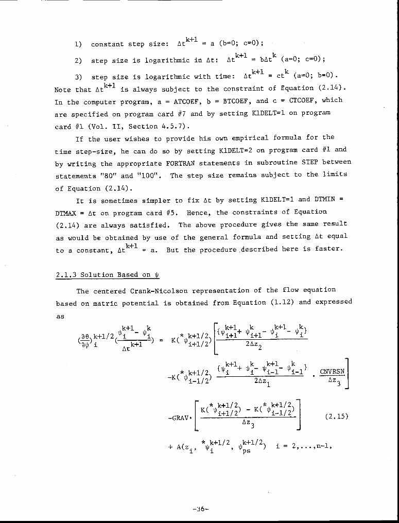
2.1.3 Solution Based on ip

The centered Crank-Nicolson representation of the flow equation

based on matric potential is obtained from Equation (1.12) and expressed

as

,k+1 k k+1 k k+1 k

30 k+1/2 4) *k+1/ 14) i+11- 4) i+1- i - 1Pi/

e5 ) i ( Atk+1 ) - K()i+1/2 2Az2

j‹.* k+1/2 ' 41i-1 CNVRSN

-K( tq..1/2)

1 J+1.1.

2Az 1Az3

* k+1/2 k+1/2+ ,) i = 2,...,n-1,

fps

-36-

where Az and At are defined by Equations (2.2) and (2.3) and where

(ae/4) is the specific water capacity, evaluated at *11+1/2. Thehydraulic conductivity function, K, is always specified by the user as a

function of water content and not matric potential. So, for the program

to evaluate K(), the following steps are taken by the computer:

i) determine the desired value of matric potential, 4),

ii) using the soil-water characteristic function 6(4)), compute the

value of water content, e, corresponding to the value of

matric potential obtained with step i),

iii) determine the hydraulic conductivity for the water content

found in step i) above, then set K(i) = K(6).

The superscript "*" indicates that the variable is an estimate.

The "starred" quantities are defined analogous to the definition of 8 in

Equation (2.4). The n-2 flow equations of Equation (2.15) for the

interior nodes and the upper and lower boundary conditions make a total

of n equations with n unknowns for time level (k+1). The initial condi-

tion is given by

k=0 = 4)0 (z i ) i = 1,...,n. (2.16)

The three upper boundary conditions, stated earlier, are backward-

differenced.

1st type:

4+1 = RHS(t

k+1).

2nd type:

k+1 k+1IP 2 - *1 1 = RHS(tk+1).z 2 - zi

4th type:

(2.17a)

(2.17b)

k+1 k k+1 k+136 k+1/2

(4) 1 1P1

) = K(*k+1 , 14) 2 - 1 ( 94) ) 1

At1+1/2 )• CNVRSNk+1

(z -zz )2

,,*,k+1 k+1wi+1/2 1 go • GRAY + . (2.17c)

(z2 zl)(z

2 - z

1)

-37-

The lower boundary conditions are finite-differenced in the same manner

as those of the water-based flow equation (Equation (2.8)).

The guessing and iterating scheme used for solving the water-

based flow equation is also used for solving the flow equation based on

matric potential. At a given time level, the flow equation is assumed

to have converged when

*gi k+1- k+1

4.)max I

ii, 1< WRATIO i= 1,...,n, (2.18)

* k+1 —Ipi

where WRATIO is the maximum allowed difference expressed as a ratio.

2.1.4 Solution Based on the Kirchhoff Transform

The Kirchhoff transform variable, F, is defined by Equations (1.16)

and (1.17) and is computed numerically by means of a numerical integra-

tion scheme in subroutines INTGRT and TRNSFM.

Several steps are taken by subroutine TRNSFM to solve Equation

(1.16) and to create a table of 20 values of F versus e.

i) Compute the transform variable F at 20 values of 8, such that

8., jr 3 D(e')dO Tj = 2,...,20, (2.19)

3 et=ed

where F(0 1) = F(ed) is defined by Equation (1.19) and where

8 = 8 + ( es-0

d)•PICK(j) j = 2,...,20.

3 d

The values of PICK(j) are given in Table 2.3.

(2.20)

ii) Numerically evaluate the integral of Equation (2.19) by sub-

dividing the interval (e e.) into 40 intermediate points,d' 3

such that

8 = + (e.—e )/39 2 = 2,...,40,9, Z-1 3 d

where at k = 1, e l = ed.

(2.21)

-38-

iii) Numerically integrate the 40 subpoint values of D(0 2 ) vs 8 ,Q, by

means of a second-order Taylor series expansion integration

scheme which allows for unevenly spaced pivotal points (Sec-

tion 3.7.2). Subroutine INTGRT returns with the integrated

values of F(0j).

iv) Repeat steps i) through iii) for all 20 values of. Theej

resultisatableofF(8 . )vs 8, which is stored in data setJ J

FW.

Table 2.3. The values of PICK(j)

j PICK(j)

1 0.00002 0.00503 0.01004 0.01755 0.02506 0.05007 0.07508 0.10009 0.2000

10 0.300011 0.400012 0.500013 0.600014 0.700015 0.800016 0.900017 0.950018 0.970019 0.990020 1.0000

The steps taken by subroutine TRNSFM to solve Equation (1.17) and

to create a table of F vs tp are listed below. The steps taken differ

from those for the solution based on 0 because the integration variable

tp can vary over several orders of magnitude. It was found by trial and

error that the procedure given below is fairly accurate and consistent.

i) Compute the transform variable F at 40 different values of

such that

F.)= CNVRSN1P4

or K(*')d*' j = 2,...,40, (2.22)(*3

*I=d

where F(* 1 ) = F(ld) is defined by Equation (1.20) and where

such that*3

e. = e. + (e s–ed)/39j = 2,...,40,

3-1

8. = 8 .3=1 d

(2.23)

ii) Numerically evaluate the integral of Equation (2.22) by sub-

dividing the interval (* .) into 40 intermediate points,d' 3such that

lni* 1 = lnl* 1 + (inky - lnl*d1)/39 Z = 2,...,40,

Z-1

*Z=1 = *d'(2.24)

iii) Numerically integrate the 40 subpoint values of K(i 2 ) vs *z

from step ii) using an integration scheme based on a second-

order Taylor series expansion which allows for unevenly spaced

pivotal points (Section 3.7.2). Subroutine INTGRT returns

with the integrated values of F(*j).

iv) Repeat steps i) through iii) for all 40 values of ^, j . The

resultisatableofF(*.)vs.which is stored in data*3

set FP. -

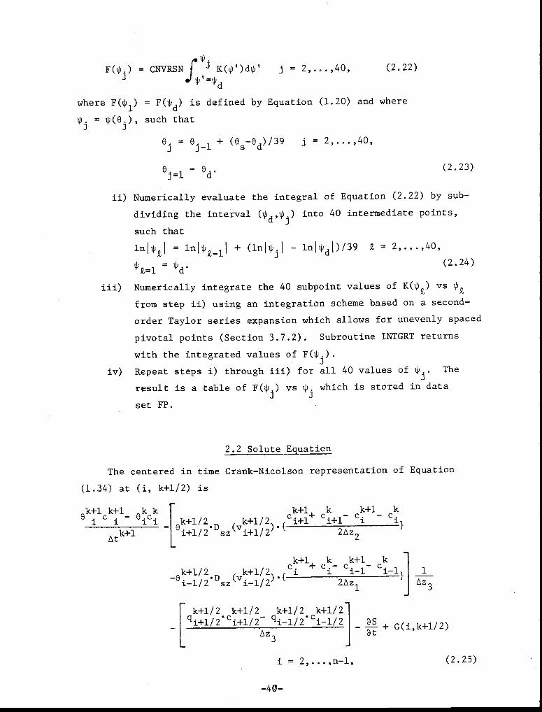
2.2 Solute Equation

The centered in time Crank-Nicolson representation of Equation

(1.34) at

k+1 k+16 c -i

(i, k+1/2)

k k8.c1 i

is

k+1/2k+1+ cc

k+1/2 i+1k -

k+1-ci+1 i

c 11

Atk+1 i+1/ sz

(vi+1/2

).{ 2Az2

k+1/2-8. . (v

k+1/2)-{

1-1/2121 sz i-1/2

k+1+ ck-

k+1-c ci i-1

kci-1

1

12Azi Az3

k+1/2 k+1/2 k+1/2 k+1/2qi+1/2'ci+1/2- –-+ G(i,k+l/2)

Az3-a

i = 2,...,n-1, (2.25)

-40-

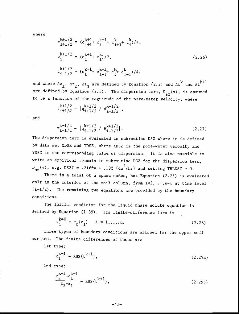
where

k+1 k+1 kk+1/2 = (c. + c. + c. +ci+1/2 1+1 1+1

k+1/2 k+1 kC. = (c i + ci)/2,1

ck+1/2 k+1 k+1 k k

i-1+ c

i+ c

i-1 )/4i-1/2

(2.26)

and where Az1, Az 2, Az

3 are defined by Equation (2.2) and At

k and At

k+1

are defined by Equation (2.3). The dispersion term, D (v), is assumedsz

to be a function of the magnitude of the pore-water velocity, where

k+1/2 1 k+1/2 k+1/21

vi+1/2 = lqi+1/2 ei+1/21'

and

k+1/2k+1/2 k+1/21vi-1/2 = lqi-1/2 / i-1/21*

(2.27)

The dispersion term is evaluated in subroutine DSZ where it is defined

by data set XDSZ and YDSZ, where XDSZ is the pore-water velocity and

YDSZ is the corresponding value of dispersion. It is also possible to

write an empirical formula in subroutine DSZ for the dispersion term,

D (v), e.g. DSZI = .216*v + .192 (cm 2/hr) and setting TBLDSZ = 0.sz

There is a total of n space nodes, but Equation (2.25) is evaluated

only in the interior of the soil column, from i=2,...,n-1 at time level

(k+1/2). The remaining two equations are provided by the boundary

conditions.

The initial condition for the liquid phase solute equation is

defined by Equation (1.35). Its finite-difference form is

k=0c. = c

0(z) i = 1,...,n. (2.28)

Three types of boundary conditions are allowed for the upper soil

surface. The finite differences of these are

1st type:

k+1 k+1c1= RHS(t ), (2.29a)

2nd type:

k+1 k+1c2

1 k+1-c

- RHS(t ), (2.29b-zlz2

-41-

2nd type:

k+1 k+1cn - cn-1 - RHS(t

k+1),z- zn n-1

(2.30b)

3rd type:

ck+1

+ ck

- ck+1- c

kek+1ck+1- e

kck

1 1 1 1 2 1 1— (eD )

k+1/2 .{ 2 }

k+1 sz 1+1/2At 2(Az 2

)2

(2.29c)k+1+ k+

k+1+ k k+1/2

ck+1/2 1 1 2

c fo 1+1q /2“ 4Az2

21 + Az

2 '

k+1/2whereis the Darcian flux, RHS(tk+1) corresponds

Az2 = z2 z1, (11+1/2to the specified value of the boundary condition at time t k+1 , and

fk+1/2 is the actual flux of solute through the upper surface as defined0

by Equation (1.37). Source/sink terms are not evaluated at the upper

surface. The user must supply the value of RHS and f through subroutine

BCCTOP.

There are also three types of boundary conditions for the lower

soil surface. The finite differences of these are

1st type:

k+1 = RHS(tk+1

), (2.30a)cn

3rd type:

k+1 k+1 8 k kk+1

+ k k+1 k

0n cn

- ncn k+1/2 c

cn- cn-1

- cn-1

— —(eD sz) n-1/2

{ 1k+1

At 2(Az )2

(2.30c)1

k+1 k k+1+ k k+1/2k+1/2 1

cn-1

+ cn-1+ cnc fnl _ n

+' qn-1/2 ' 4Az1 Az1

where Az1 = z

n - z

n-1' and where

fk+1/2 is the actual flux of solute

through the lower surface as defined by Equation (1.37). The user sup-

plies the values of RHS and f through subroutine BCCBTM.

The sorption terms are finite-differenced by means of the centered

Crank-Nicolson method. These are listed in Tables 2.4 and 2.5, where

-42-

* k+1 kS.-S.

9S i i _at

Atk+1

k+1/2 k+1c. = (c i + c ik)/2,

k+1/2 k+1Si+l/2 (S i + Si)/2.

(2.31a)

(2.31b)

(2.31c)

Without sorption and the source/sink terms, Equation (2.25) is

linear with respect to concentration, c. The non-linearity induced by

the sorption term requires that Equation (2.25) be solved by iteration

(Sections 3.5 and 3.6).

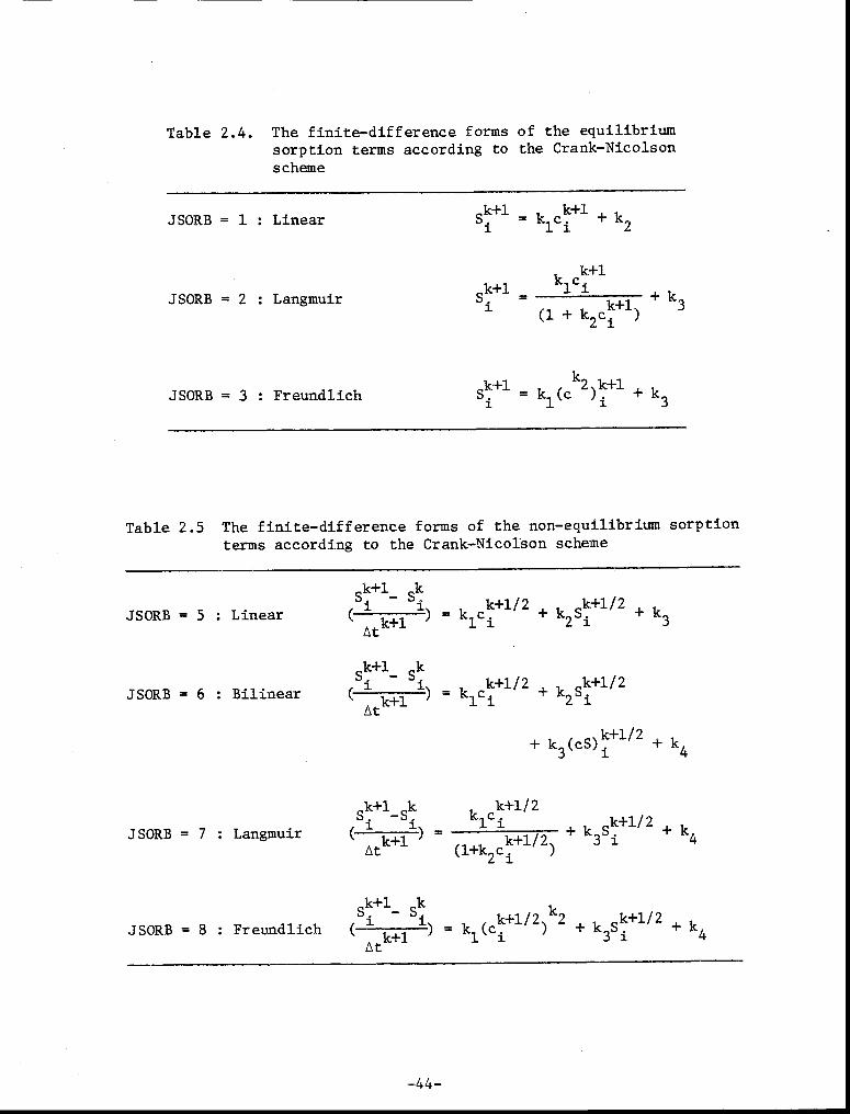
Table 2.4. The finite-difference forms of the equilibriumsorption terms according to the Crank-Nicolsonscheme

JSORB = 1 : Linear

JSORB = 2 : Langmuir

JSORB = 3 : Freundlich

Sik+1 k+1+l k

1ci + k2

k+1k+1

- k1c

S1(1 + k2 c

k+1) + k

3

k+1S.=k1

(ck2

)k+1

+ k31

Table 2.5 The finite-difference forms of the non-equilibrium sorptionterms according to the Crank-Nicolson scheme

JSORB = 5 : Linear

JSORB = 6 : Bilinear

k+1kf S 1. -

S1) k+1/2

1) - k1ci+ k2

Si

+ k3` At

k+1

k+1 kS. S. k+1/2 k+1/2

At

f 1 1) = k c. + k S.` k+1 1 1 2 1

+ k3(cS)

k+1/2 + k4

JSORB = 7 : Langmuir

k+1 k k+1/2S. -S. k c.1 1 kf 1 1) = + k S+1/2. + k4k+1/2 3 1` Atk+1 / (1+k c. )2 1

k+1- k.

JSORB = 8 : Freundlich(S1 1) k (c.

k+1/2 )k2 + k S.

k+1/2 + k4

Atk+1

S

1 3 1

-44-

3. ITERATION ALGORITHMS

3.1 Methods of Iteration

The computer program uses three basic methods of iteration in

solving the water and solute flow equations, namely:

a) successive averaging,

b) Newton-Raphson iteration,

c) Golden Section Search.

Iteration is required when the equation to be solved is a non-linear

function of the dependent variable. The flow equation based on water

content contains the non-linear functions of diffusivity, conductivity,

and surface flux. The mass transport equation may have non-linear

sorption and/or desorption terms. The iteration process may be thought

of as a method of finding the roots of a transcendental equation.

3.1.1 Successive Averaging

With the successive averaging approach, successive estimates are

made of the dependent variable (e.g., water content) by averaging the

most recent computed value with the previous estimate so that

new guess = (old guess + computed value)/2. (3.1)

The rate of convergence of this technique is usually very rapid, but

depends a great deal on the first estimate. The linear extrapolation

technique

Atk+1

xk+1 • (xk-xk-1),= xk + ACLRAT •Atk

(3.2)

usually gives an excellent first guess for time level (k+1).

The method of successive averaging is usually reliable but it can

fail to converge. This occurs when the iterator enters a repeating

guess-compute cycle. Table 3.1 shows an example where the estimated

and computed values of water content repeat every second iteration.

-45-

Table 3.1. Example of a guess-compute failure in thesuccessive averaging method

Iteration

0 (guess) 0 (compute)

64 .3805E-01 .3563E-0165 .3684E-01 .3950E-0166 .3817E-01 .3537E-0167 .3677E-01 .3932E-0168 .3805E-01 .3563E-0169 .3684E-01 .3950E-0170 .3817E-01 .3537E-01

The conditions that lead to a repeating guess-compute cycle are not

known beforehand. This type of failure occurs only on rare occasions.

To eliminate this uncertainty, however, the successive averaging method

has been replaced in the computer program described in this report by

the Newton-Raphson technique. When the successive averaging method is

used, it is restricted to only the first several iterations. The com-

puter then switches to the Newton-Raphson scheme.

3.1.2 Newton-Raphson Iteration

The Newton-Raphson technique of iteration is based on a first-order

Taylor series approximation of a function whose value is approaching

zero.

H(x+dx) = H(x) + —aH

dx 0.ax

(3.3)

A new guess is defined by solving Equation (3.3) for dx, such that

xm+1

(new guess) = xm(old guess) + dx, (3.4)

where

dx = -H(x)/(aH/Dx) (3.5)

The Newton-Raphson method of iteration is very fast. It has a

second-order rate of convergence in the neighborhood of the final

solution. However, the method can diverge if the initial guess is too

far from the final solution. It is, therefore, best to start out by

using the linear extrapolation technique (Equation 3.2).

At the start of a new time step, program OR-NATURE uses the linear

extrapolation technique to make the initial guess. On the next few

-46-

iterations OR-NATURE uses the successive averaging technique. During

the final iterations, OR-NATURE uses the Newton-Raphson method until

convergence is reached.

3.1.3 Golden Section Search

The most sophisticated technique for iteration used in the computer

program described in this report is the so-called "Golden Section

Search" method. It is a special case of a Fibonnaci Section Search. A

detailed description is presented in reviews by Aoki (1971) and by

Jacoby et al. (1972). It can be shown that given the total number of

times that a function is to be evaluated, a Fibonnaci Section Search of

a unimodal function is optimal. It minimizes the maximum possible

interval of uncertainty in which the minimum of the function lies.

The Golden Section Search method to determine the location of the

minimum of function H consists of several steps (Figure 3.1).

Step a) Choose two values a and b of the independent variable which0 0bracket the minimum of function H. The initial interval of

uncertainty in locating the minimum of function H is now

defined as [ao,b0].

Step b) Compute the values of the interior points

xl = ao + .328(b 0 - a0),

xi = al) + .618(1)0 - a0 ), (3.6)

and evaluate function H at the points x l , xi. Set the itera-

tion index m = 1 and am =a b =b and proceed with the0' m 0

next step.

Step c) There are two possible results of step b)

i) If H(xm) is less than or equal to H(x') the next interval

of uncertainty is chosen as [a b ] such thatm+1' m+1am+1 = am,

= 'bm+1 xm'

x = xm' and1

xm+1 = am+1 + .328(bm+1 am+l). (3.7)

-47-

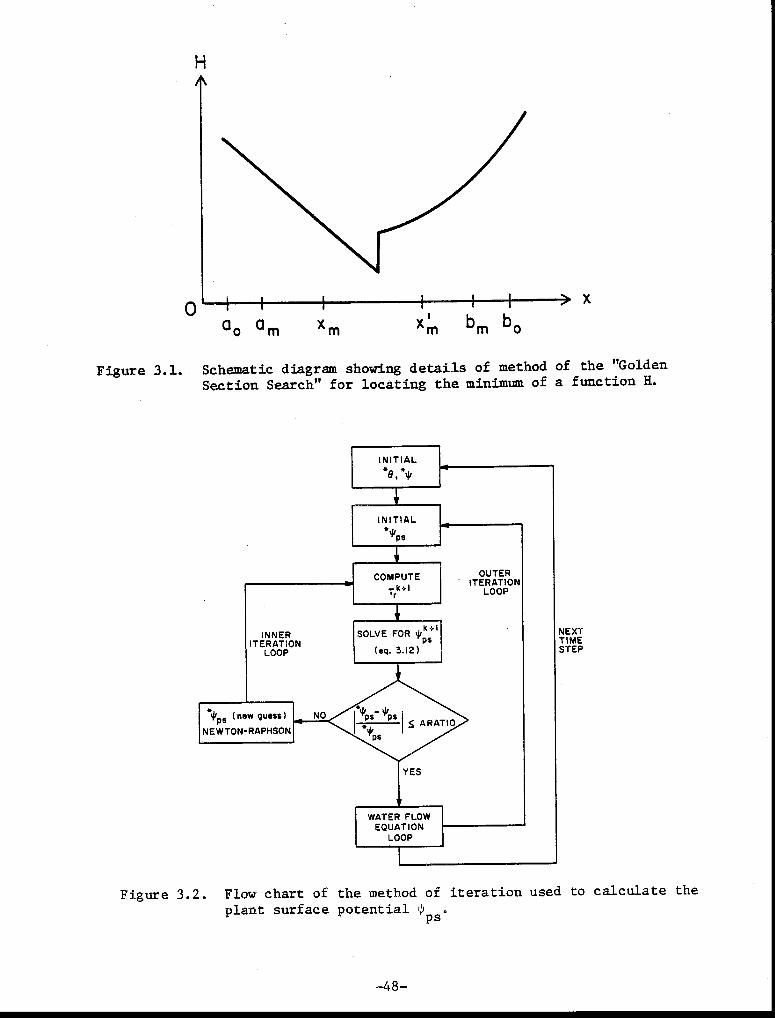
X0x'm bm boa a m x mo m

.11INITIAL.8,.*

INNERITERATION

LOOP

INITIAL..tkps

COMPUTEIrk+1

SOLVE FOR lit k+ I

(eq. 3.12)Ps

WATER FLOWEQUATION

LOOP

OUTERITERATION

LOOP

Nips (new guess)NEWTON-RAPHSON

Figure 3.1. Schematic diagram showing details of method of the "GoldenSection Search" for locating the minimum of a function H.

Figure 3.2. Flow chart of the method of iteration used to calculate theplant surface potential fps

.ps

NEXTTIMESTEP

-48-

Evaluate the value of H(xm+1 )' then set m = m+1 and

return to the beginning of step c).

ii) If H(xm) is greater than H(x'), the next interval of

uncertainty is chosen as [a , b m+1

] such thatm+1

am+1

= Xm

bm+1

= bm

xm+1

= x'' and

m

xM+1 = am+1 + .618(b

m+1 am+1)*(3.8)

Evaluate the value of H(x' ) set m = m+1 and return tom+1 '

the beginning of step c).

Step d)

The iteration procedure of step c) ends when the interval of

uncertainty is reduced to some specified ratio of the original

interval by the statement

bm+1

- am+1 stop if ( ) < QRATIO. (3.9)13 0 - a0—

Test points x and x' m m'n are always within the interval [am

(Figure 3.1). However, during any given iteration, the program evalua-

tes function H at only one of these points, the other points having been

evaluated on the previous iteration. Thus, only one evaluation of

function H is required per iteration.

The Fibonnaci Section Search is the most efficient no-derivative

line search procedure that guarantees a prescribed accuracy. The only

condition required is that the function H be unimodal in the interval of

the search. Except for this unimodal property, which is normally

satisfied in some neighborhood of a minimum, the function may be

irregular and discontinuous.

The interval of uncertainty, i.e., the location of the minimum of

function H, is reduced very rapidly. The interval of uncertainty is

reduced to one percent of the original interval in 11 iterations. In

general, the interval of uncertainty on the m-th iteration is approxi-

mated by the formula

-49-

(b -a )0 0

(bm-a

m) =

FB1

where the Fibonnaci numbers FBm are defined by

FB =FB+m = 2,...,00,m m-1

(3.10a)

(3.10b)

and where

FB = FB1 = 1. (3.10c)

0

Thus, on the eleventh iteration, FB11=144 and (b -a )/(b -a ) = .007.

10 10 0 0

The number of iterations required to compute the minimizing value

of a function to accuracy QRATIO is the greatest integer less than or

equal to

In (QRATIO) 1 + [

ln(1-c)

where c = (3-I) /2 = .381966.

(3.10d)

3.2 Algorithm to Compute the Plant Surface Potential

To evaluate the root sink model as stated by Equation (1.52) at

time level (k+1/2), the plant surface potential, 1pk+1/2 must be deter-ps

mined. However, the plant surface potential depends on the potential

transpiration demand, the potential surface flux, the soil matric poten-

tial, and the root distribution. The correct value of ip for a givenpstime step is found with an iterative algorithm.

1) Make an estimate of water content * 0k+1/2 , from Equations (2.4b)i

and (2.10b) and an estimate of water potential, *Ipk+1/2 , whereik+1

*k+1 = k + ACLRAT (At

k )(1P i - k-1 ),At-

(3.11a)

and

* k+1/2k * k+1= (4) 1,. + )/2, (3.11b)

for i = 1,...,n at time level (k+1/2).

Make an initial estimate of the plant surface potential by linear

extrapolation from the previous time step,

-50-

0k-1/2* k+l/2 = k-1/2

+ ACLRAT(Atk+1

) - k-3/ 2).

ps psAt

k ps ps(3.12a)

3) Compute the actual rate of transpiration, Tk+1/2,

based on therestimated plant surface potential and the potential rate of trans-

piration as described by Equation (1.41).

4) Set the actual transpiration demand of step 3) equal to the sum of

the root sinks according to Equation (1.53) and solve for the plant

surface potential. This is the computed value of ip k+1/2

k+1/2ps

ps

Tr( n-1

- i=2 2 [Ks -RAF..(z.+RPF -

*k+1/2.CNVRSN) . ( )]ir ps ys,i i 2

n1 z zi+1 i-1 E [K ).CNVRSN]i=2 sys1 2

(3.12b)

whereKsysx mF ., 1andu *F.are evaluated with values of e i

k+1/21

5) Compare the estimated and computed values of the plant surface

potential. Convergence is reached when the ratio

* k+1/2k+1/2-ps ps

* k+1/2ps

< ARATIO, (3.13)

where ARATIO is the specified convergence ratio. The iterator

stops when Equation (3.13) is satisfied. At that time, the program

proceeds to solve the water flow equation.

6) If a satisfactory degree of convergence is not obtained in Step 5),

make an 2*improved estimate of k+1/ by means of a Newton-Raphsonps

iteration scheme. For this scheme, define the optimization

function H as the difference between the computed and guessed

values of plant surface potential

H = *k+1/2k+1/2-ps ps (3.14)

The objective is to iterate on *k+1/2 until H goes to zero. Theps

derivative of H must be evaluated as a function of the guessed

-51-

value, specified by Equation (3.3). The superscript k+1/2 of

Equation (3.14) is dropped for convenience in further discussions.

911 90Pps )*

= 1 - (3.15)

a( )a( ps ) ps

The second part of the right side of Equation (3.15) is obtained by

differentiating Equation (3.12b), thus,

a(q) ) 9(T(T)ps r

a( fps)a( fps 1 . (3.16)

n-1 z - z.E K

i+1 1-1)-CNVRSNRAF.

sys .,1 2

Using Equations (3.4) and 3.5), an improved estimate of the plant

surface potential is made by

*k+1/2(new guess) =

*k+1/2(old guess) -

ps psDH/9 ps

(3.17)

(old guess)

where H is evaluated by using Equation (3.14) and the derivative by

using Equations (3.15) and (3.16), all evaluated with the old

guessed value of *k+1/2

ps

7) Return to Step 3). The iteration algorithm of steps 3) to 6)* k+1/2

continues for fixed values of Ai

until Equation (3.13) is

satisfied. If the new estimate of **k+1/2 from Equation (3.17)ps

violates the feasibility condition of Equation (1.42), then set* k+1/2

to the limiting value.ps

If *k+1/2

> 0,ps

set *k+1/2

= 0.ps

(3.18)

8) If the final converged value of If,k+1/2

< the plant isps - wilt'

assumed to be permanently wilted and dead. When wilted, transpira-

tion and root uptake stops and the program no longer computes ,ps

A(i) or G(i).

The algorithm of steps 1) through 7) above requires the solution of

two sequential iteration schemes called the "inner iteration" and "outer

iteration" (Figure 3.2). Each time a new estimate is made of the water

content, *k+1/2, during a given time step, the program must first solve

program must first solve the inner iterator routine which consists of

steps 3) to 6). In the inner iterator, the program hunts for a value of* k+1/2

for fixed values of * 0k+1/2

. Once a feasible value of *k+1/2

ps psis found, the program enters the outer iteration routine. The outer

*iteratorrator finds an improved estimate of 0i

p

k+1/2 for a fixed value of*k+1/2

. This sequential process continues back and forth until both

* k+1/2 * k+1/2and

icoverage.ps

3.3 Algorithm to Compute the Water Content

The water content must be estimated by iteration to evaluate the

non-linear coefficients A, D, and K in Equation (2.1). Subroutine WATER

uses the successive averaging technique on the first three iterations

and then switches to a Newton-Raphson iteration scheme. In the Newton-

Raphson scheme, the optimization function H is defined as the difference

between the computedik+1 and the guessed *

ik+1 at node i,

* k+1 k+1H.

i= -

i = 1,...,n. (3.19)

*The objective is to iterate on eik+1

until Hi goes to zero for each

node. In the following discussion, the subscript i will be dropped, but

it is to be understood that the iterator scheme is simultaneously

applied to each node. The superscript k+1 is also omitted, since all

values of 0 are being evaluated at the future time level (k+1).

Function H is expanded by a Taylor series to the first-order about

the previous guess

* * 31-1H( e+d e) = H(*0) + * • d

*0 = O. (3.20)

a 0

The derivative of H in Equation (3.19) with respect to*

8

aH DO= 1 -* *

D 8 D e

is finite-differenced between iterations m and m-1 as

311 em - em-1= 1* m * m-1

).9 0 0 - e

(3.21a)

(3.21b)

-53-

The correction d A is solved from Equation (3.20) such that

d-H

8 = * •ax/a8

(3.22)

Upon substitution of Equations (3.19), (3.21) and (3.22) into

(3.4), an improved estimate of water content is obtained by

* Om - Om)*em1

(new guess) = *em(old guess)

( em em-1

[1-(* m* m-1)]- 8

wherethenotation 11 8m+1 =ande=The following1

algorithm is used to compute the water content in subroutine WATER. A

schematic diagram for the scheme is given in Figure 3.3.

1) Make an initial estimate of the water content for time level (k+1)

by linear extrapolation from the previous time step, using Equation

(2.10).

2) Compute the surface water flux , q0

k+1

by means of the Golden Section

Search routine if a fourth type boundary condition is specified on the

upper surface (Section 3.4).

3) Compute the plant surface potential, IP kps

1/2, using the Newton-

Raphson scheme given in Section 3.2.k+1 *,k+1,

4) Evaluate the tri-diagonal matrix coefficients using q0 ,

and IPk+1/2

in Equations (2.1) to (2.9). Solve the tri-diagonalps k+1

matrix by the Thomas algorithm and compute e. .

5) If any of the newly computed values of 0k+1 violate the feasibility

conditions of Equation (1.4), set them to the limiting value.k+1 k+1

01").<0 1P sete ' = d'1i = 1,...,n. (3.24a)

+1110 .

k>es,setel.

k+1 =0s'i = 1,...,n.1 1

(3.24h)

Compare the estimated and computed values of water content by

means of Equation (2.12).

7) If a satisfactory degree of convergence is obtained in step 6) at

all nodes, the water content algorithm ends and the program pro-

ceeds to the next time step or to the Golden Section Search routine

to find an improved estimate of the surface flux if the upper

boundary condition is described by a flux type.

(3.23)

-54-

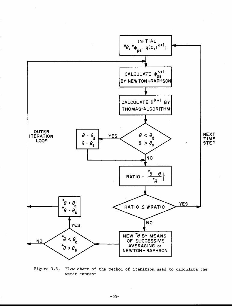
INITIAL, q(0,tk+I)

NO

RATIOS WRATIO

NEW e BY MEANSOF SUCCESSIVEAVERAGING or

NEWTON - RAPHSON

OUTERITERATION

LOOPNEXTTIMESTEP

Figure 3.3. Flow chart of the method of iteration used to calculate thewater content

-55-

8) If a satisfactory degree of convergence is not obtained in Step 6),* k+1

a new estimate of 6iis made. During the first three iterations,

a new estimate of water content is made by means of the successive

averaging scheme given by Equation (2.11). Proceed to Step 9) at

the end of each of the first three iterations. After the fourth or

successive iterations, a new estimate of water content is made by

means of the Newton-Raphson scheme of Equation (3.23).

9) If the new estimates of water content from Step 8) violate the

feasibility conditions of Equation (1.4), set them to the limiting

value.

* k+1 * k+1Ife.<0sete.=0

d'1 d' 1

* k+1 * k+1=If 0.>0

s' set O.

s'el+l

i = 1,...,n.

= 1,...,n.

(3.25a)

(3.25b)

Return to Step 3).

The algorithm to solve the water flow equation is the same, regard-

less of whether the problem is solved in terms of 6 (volumetric water

content), tp (metric potential) or F (diffusivity potential).

3.4 Algorithm to Compute the Surface Flux of Water

To solve the flow equation based on water content with a flux type

boundary condition (4th type) on the upper surface, one must specify the

potential flux, R(0,t). Water infiltrates the soil as fast as supplied

as long as the rate of supply to the surface is smaller than the rate of

infiltratability. Hillel (1971) calls this flux condition as being

"flux-controlled". When the rate of supply exceeds the rate of infil-

tration, it determines the rate of infiltration. Hillel (1971) refers

to this flux condition as being "profile-controlled". The same terminology

is used to describe water flux during evaporation.

When the surface flux is flux-controlled, the actual flux equals the

potential flux

qk+1

= R(0,tk+1

).0 (3.26)

The solution to the water flow equation under this condition is straight-

forward. Substitute Equation (3.26) into the right side of the boundary

-56-

Qc(computed

[feasible] [unfeasible]

a(correct)

Qg (guessed)b R(o,t)

Figure 3.4. Conceptual diagram of the method used to determine convergence of the iterator forcalculating the flux of water at the soil surface.

condition of Equation (2.6c). When the surface flux becomes profile-

controlled, the magnitude of the actual flux is less than that of the

potential flux, thus

1,k+1I < IR(0,tk+1 )1. (3.27)

140

The actual flux is not known beforehand and an iterative algorithm must

be used to find it. The solution to this problem is not trivial, but it

has received little attention. In fact, Neuman et al. (1975) seem to be

the only authors who attempted to describe this problem with any degree

of completeness.

Two major difficulties are encountered in solving the profile-

controlled problem. These are defining an appropriate criterion that

indicates when the correct flux has been found by an iteration scheme

and finding an iterator scheme that is not time consuming. The actual

surface flux is subject to the condition that its magnitude be as large

as possible but not greater than the potential flux according to Equa-

tion (3.27). In addition, the resulting water content profile must not

violate the air-dry and saturation limits given by Equation (1.4).

Figure 3.4 shows schematically a method for determining the actual

surface flux. Figure 3.4 is constructed by plotting the guessed values

of flux versus the computed values of flux. In the feasible range, the

guessed and the computed values of flux are equal. In the unfeasible

range, the guessed and the computed values of flux differ. The latter

condition occurs only when a computed value of water content in one or

both of the two top nodes is unfeasible and is set to either an air-dry

or saturated value.

The iteration scheme used to find the correct surface flux is that

of the Golden Section Search method.

1) The initial interval of uncertainty in finding the actual flux is

defined as ja0 ,b0 ] where

a0 = 0,

b = R(0,tk+1

),0

with intermediate test points

xo = a0 + .328(b0-a0),

xO = a0 + .618(b0-a0),

-58-

and the initial guess of the surface flux given as

Q = b = R(0,tk+l

).g 0

2) Make an initial guess of the water content, *ek+1,

for time level

(k+1) by linear extrapolation from the previous time step using

Equation (2.10).

3) SubstituteQand * 8 1,4-1 into the coefficients of the finite-g

difference equations 2.1, 2.6c, and 2.8c, where qk+1

= QQ.0

4) Solve the resulting tri-diagonal matrix of Step 3) by the Thomas

algorithm.

*+15) Holding Qg fixed, iterate on the values of water content eki

by

means of the successive averaging and the Newton-Raphson techniques

until *k+1 and ek+1

converge. The water content is always re-

stricted between air-dry and saturation, as in Equation (3.25).

This last step must be completed before proceeding to Step 6).

6) Compute the surface flux by solving for Q c from the backward-

differenceexpressionofEquation(2.60usingthealues from1

step 5),

k+1 k+1(e 1k+1

—e 1k

)* k+1 fe 2 - e1 1

Qc = k+1(z

2 - z

1) - D( e

1+1/2)

(z2 z 1 )At

* k+1K( 61+1/2) -GRAV, (3.28)

k+1where 8.

1* k+1

and 0. are the most recently guessed values of water content.

7) If Qg Qc or if in step 5), the computed water content of one of

the top three nodes is either greater than saturation or less than

air-dry (i.e., the computer program sets MQFAIL = I, where I is the

node that failed), then the magnitude of Q g is too large and must

be reduced. The new interval of uncertainty is chosen as jam

bm+1

]

such that

am+1

= am'

= x'bm+1 m'

x' = xm+1 m'

are the most recently computed values of water content

–5 9-r

xm+1

= am

4.1 + .328(b

m+1 - a

m+1).

In other words, the upper limit is moved to a lower value and the

new flux guess is taken as

Qg = x

m+1.

Go to Step 9).

If Qg = Q

c, the guessed flux is in the feasible range but it might

not be as large as possible. Q should be increased in magnitude.g

This is described in the following steps. The new interval of

uncertainty is chosen as [am+1'

bm+1

] such that

am+1

= Xm'

bm+1

= bm'

= x'xm+l m'

xl.1+1 = am+1 + •618(bm+1 - am+1).

In other words, the lower limit is moved to a higher value and the

new flux guess is taken as

Q = x' .g m+1

9) After each iteration, plot the guessed flux Q versus its computedg

value, Qc'

according to Figure 3.4. This step is not actually done

by the computer program but the user may wish to do this as a con-

ceptual aid in understanding this routine. The correct flux lies

at the point of bifurcation or separation in the conceptual diagram

of Figure 3.4. The correct flux is the flux with the largest

feasible flux. Since an iteration scheme is being used to find the

correct flux, the final solution will only be known to lie within

some specified interval of uncertainty, given bybm+1

- am+1

< QRATIO. (3.29)Qg I

If Equation (3.29) is not satisfied, return to Step 3). Iteration

is continued until Equation (3.29) is satisfied. The convergence

criteria, QRATIO, is a ratio specified in parameter card #4. Typi-

cally, one would set QRATIO = .01 (one percent).

In subroutine WATER, the variables used in steps 1) through 9)

above are defined as:

bm+

Qc

Qg

R(0,tk+1

= QGAK,

= QGTK,

= QGTKP,

= QGBK,

= QC,

= QG,

= pp.

The iteration scheme using the Golden Section Search of Steps 1)

through 9) can fail to converge, depending on the magnitude of the

potential flux, the diffusivity function, the size of the time step, or

the size of the space step. The most sensitive step is that of the

initial guess of water content, *ek+1

, in Step 2) and the subsequent

water content guesses during the first few flux iterations. If too*+1large a change is made in guessing e

ki

, the program will fail to

converge and Qg Qc. It is not possible to know if this condition

(i.e., Qg Qc) is caused by an incorrect estimate of the flux guess or

by a too large change.

3.4.1 Modifications of the Golden Section Search Method

Through trial and error, a method was found which is effective in

eliminating the various "starting" problems associated with the Golden

Section Search. This method is used to start the first four flux itera-

tions. From the fifth flux iteration on, the regular Golden Section

Search is followed.

The modified iteration scheme consists of Steps 1) through 6) as

described above. Then a different procedure is followed.

7a) At the end of the first flux iteration of Step 6), feasibility is

checked.

k+1i) If Q is feasible and if ek+1l '

6 2

k+1g

63

are feasible, then

set

-61-

am+1

= Qg

bm+1 = b

and the program proceeds to step iii).

ii) If either Qg, e

lk+1

, 6 2k+1

or 83k+1 is unfeasible, then set

am+1

= am'

bm+1 = Qg,

Q = Q •g g

Return to Step 3) of the Golden Section Search.

iii) The next guess for the flux is given as

Qg = am+1 + .328(bm+i-am+1).

Return to Step 3) of the Golden Section Search.

8a) At the end of the second flux iteration of Step 6), feasibility is

checked.

iv) If Qg is feasible and ifk+1

,k+1

,k+1

are feasible, then1 2 3

set

am+1

= Qg'

bm+1

= b

xm+1 = am+1

+ .328(bm+1 - am+1),

= am+1 + .618(bm+1 - am+1),

and the program proceeds to step vi).

k+1 k+1 k+1v) If either Qg'

81 , 62

or e3

is unfeasible, then set

am+1 = am,

bm+1

= bm'

xm+1

= am+1 + .1(bm+1 - am41),

x'm+1

= am+1

+ .2(bm+1

- am+1

),

and the program proceeds to Step 6

vi) The next estimate of the flux is given as

Q = x'g m+1.

Return to Step 3) of the Golden Section Search.

-624-

9a) At the end of the third flux iteration of Step 6), set

am+1

= am'

bm+1 = bm,

xm+1

= xm'

_xm+1

- xm

,

Qg = xm+1.

Return to Step 3) of the Golden Section Search.

10a) At the end of the fourth flux iteration of Step 6), return to steps

7) through 9). On the fifth and subsequent iteration, follow Steps

1) through 9) of the Golden Section Search until convergence is

reached, as specified by Equation (3.29).

3.4.2 Mini-Iterator

The Golden Section Search scheme involving Steps 1) through 9) and

Steps 7a) through 10a) as described here is very accurate. But it is

very time consuming, particularly if the number of spatial nodes is

large. The top 10 nodes usually have the most influence in the

determination of the magnitude of the surface flux. It was determined

by trial and error that a sliding scale approach may be used-. In the

start of each new time step, the flux iterator algorithm uses only the

first 10 nodes at the top of the soil column to evaluate the water

content. After each additional flux iteration, only the top (10 +

IWORST) nodes are used. IWORST is the node at which the largest

difference occurred between computed and guessed values of water con-

tent. The location of the spatial nodes does not change during this

procedure, only the number of nodes at which the water content is being

evaluated. The Golden Section Search is accelerated by the following

steps, which are shown schematically in Figure 3.5.

a) Set NMINI = min110,n1, and the index of iteration m = 0 and* k+1,m=0

make an initial guess of water content, e

b) Use the Golden Section Search scheme described previously in

Steps 1) through 9) and Steps 7a) through 10a), but solve the

flow equation based on water content using only the top NMINI

-63-

spatial nodes. At node NMINI, specify a first type boundary

condition such that e(NMINI) is held fixed to its guess

during the water content iteration:

k+1,m+1 * k+1,mNMINI = 8NmIN'.

The program continues to iterate until all NMINI water content*

values, 8ki+1,m , converge and the surface flux iterator con-

verges. At the end of each iteration, set m = m+1.

c) Using the NMINI values of water content and the flux computed

in Step b as an initial guess, solve the water flow equation

using all n nodes. The proper lower boundary condition must be

used. The initial guess is taken as

* 0k+1,m+1 *ek+1,m i=1,...,NMINI,

obtained from step b, and

* k+1,m+1 * k+1,m=00. = 8 1 i=NMINI+1,...,n1

where the RHS of the above expression is the most recent

guessed value, from Equation (2.10) or Step e).

d) If the computed and guessed values of water content and flux

agree in Step c), the program has converged for this time step.

e) If the computed and guessed values of water content and flux do

not agree in Step c), then set

* ek+1,m+1 U,k+1,m i=1 ,...,n=

as obtained from Step c, and

NMINI = minIIWORST + 10, nl.

Return to Step b, using the new value of NMINI, and

* ek+1,m+1

Step b) is called the "mini-iterator" and Step c) the "maxi-iterator."

Under most conditions, this method will require 1 to 20 mini iterations

and 1 to 3 maxi iterations per time step. If the maxi-iterator is used

by itself as indicated in the original Golden Section Search scheme, 1 to

20 iterations per time step are needed. Hence, the mini-maxi approach

reduces the computational time by at least an order of magnitude, assuming

-64-

INITIALGUESSED VALUES

OF *8;

and q(0,t k+1si

-''.7.7.77:77.77.77:777.77.77.777771• -▪ - - •

tlips ITERATOR t61

CALCULATION

•RAPHSON: 'ITERATION

• FL IYX ER ATOR

or SUCCESSIVEor NEWTON-RAPHSON

ITERATION

•::CONVERGENCE::• if.s NEW:TON:—

YESe l or tki ITERATOR

Figure 3.5. Flow chart of the method of iteration used in the calcula-tion of the water flux at the soil surface.

–65–

a problem involving 100 nodes is being solved, or to state it another

way, 10 mini-iterations require approximately the same computational

time as one maxi-iteration.

Initial examination might suggest that the mini-iterator would give

very poor results since it only solves the flow equation based on water

content at the top NMINI nodes and it specifies an arbitrary lower

boundary condition. However, in practice, the mini-iterator works very

well. The mini-iterator is only used to decide if a guessed flux value

is either feasible or unfeasible. Only the top several nodes are needed

to make this decision. Once the Golden Section Search routine locates a

possible flux solution, the maxi-iterator is used to correctly determine

the water content of all nodes. The mini-iterator does most of the

work, and is also the quickest. The mini-iterator provides a "coarse

adjustment" and the maxi-iterator gives a "fine adjustment" to the

Golden Section Search technique.

3.5 Algorithm to Compute the

Liquid Phase Solute Concentration

In the absence of any source/sink terms, the solute displacement

Equation (1.34) is linear and no iteration scheme is needed to obtain

the liquid phase solute concentration, ck+1

. However, if there is a

source/sink term, G, the solute displacement equation becomes non-linear

if G is a non-linear function of ck+1/2 (Section 1.5). Since the

magnitude of the source/sink function is normally small in comparison to

that of dispersion and convection, the procedure adopted here is to

approximate the G term and treat the solute displacement equation as if

it is linear. The computer program uses a guessed value of*

concentra-

tion, c ik+1 , in the evaluation of the G term. The program guesses

* k+1c. using a linear extrapolation such that

k+1*ck-1-

+ ACLRAT(At

k )(c - c.

k-1 ) i=1,...,n. (3.30)

At

-66-

k+1/2Substitute *c from Equation (3.31) into Table 1.5 to evaluate

GCOEF. The source/sink term G(i) is defined

*Sk+1/2* k+1/2 k= ( S

(3.31a)+ S)/2

* k+1/2 * k+1 kc i= ( ci+ ci)/2 (3.31b)

k+1/2 * k+1/2 * k+1/2 k+1/2Passive: Gi = GCOEF(c. S. ).A (3.32a)1 1 i

Active: G.k+1/2 * k+1/2 * k+1/2= GCOEF ( ci, Si) (3.32b)1

at the (k+1/2) time step by substituting Equation (3.31) into Equation

(1.54) to get Equation (3.32). The resulting tri-diagonal matrix of

Equations (2.25), (2.29) and (2.30) is solved by the Thomas algorithm

forthenvaluesprimprogramwmnotiterateareven if

this value is not identical to the guessed value *ck+1

. Since the

numerical contribution of G(i) is small, the guessed value is not much

different from the computed one and this approximation gives good results.

However, a slight modification is made to update the guessed value

of *ck+1

when a sorption model is included in the solute displacement

equation (Section 3.6).

3.6 Algorithm to Compute the Sorbed or

Solid Phase Solute Concentration

When specifying a sorption term in Equation (1.34), the solute

displacement equation becomes a function of the two dependent variables,

c -1-l andsil .The liquid phase of solute at time level (k+1) and node1 1iisdefinedbyvariableand the sorbed phase by variable S. +1

1For each of the space nodes, one must specify two equations, namely the

transport equation of Equation (1.34) and the sorption model (Tables 1.3

and 1.4). Typically, one would solve these 2n equations simultaneously.

An alternative method is to use an iterative algorithm where one of the*+1dependent variables, Ski , is assumed to be known for a given time

level and the remaining variable, ck+1 , is then obtained by the Thomas

-67-

algorithm as in Section 3.5. An iterative procedure is used to improve

on the guessed value of *Sk+1 and the procedure is repeated until reaching

a specified convergence criterion. No iteration is required when using

a linear equilibrium sorption term (e.g., JSORB =1). The iteration

algorithm is as follows:

1) Make an initial guess of *Si using the linear extrapolation '

technique, where

*Ski+1 = S + ACLRAT (

Atk+1)(S

k - S

k-1) i=2, , n-1 (3.33)

Atk i i

assuming that there is no sorption at Nodes 1 and n.

If there is a source/sink term, the coefficient GCOEF(i) is

evaluated using an approximated value of concentration, * i '

obtained by a linear extrapolation technique as given by

Equation (3.30). The source/sink term, G.k+1/2 is then deter-

mined using Equations (3.31) and (3.32) with GCOEF evaluated* k+1/2 * k+1/2

at c. and Si

3) The sorption term is obtained by finite-difference methods

such that

33S

(-) ='t .

3.

* k+1 k

Atk+1

i=2,...,n-1 (3.34)

where ll is the most recently guessed value of sorption at

nodei.Sk:is the computed value of sorption at node i, time

level (k). There is no sorption allowed at Nodes 1 and n.

4) Substitute the value of G(i) from Step 2 and (9S/3t) i from

Step 3) into Equation (2.25).

5) Specify the upper and lower boundary conditions for the solute

equation, using Equations (2.29) and (2.30).

6). Evaluate the tri-diagonal matrix of coefficients of Equation

(2.251 and solve for ck+1

, i = 1,...,n by the Thomas algorithm.

7) Use the computed values of ck+1 to recalculate the solid phase

solute concentration Sk+1

asfollows:

i) If sorption is modeled as an equilibrium process, backward-

difference the sorption model at (i,k+l) and solve for

sk4-1 (Table2.01411erecis taken from Step 6).i

-68-

ii) If sorption is modeled as a non-equilibrium process,

finite-difference the model by a centered-in-time Crank-

Nicolson scheme at (i,k+l/2) and solve for Sik+1

(Table 2.5)

whereck+1

is taken from Step 6).

8) The routine converges for this time step when

max

* k+1 k+1S,1

< SRATIO i=2,...,n-1 (3.35) *sk+1i

where SRATIO is the convergence criterion, specified as a

ratio. A one percent criterion is set by specifying SRATIO = .01.

9) If a satisfactory degree of convergence is not obtained in

Step 8), new estimates of *Sk+1

and *ck+1

are made. An

improved estimate of the concentration of solute in the liquid

phase is made by setting the estimated value equal to that of

the most recently computed value

* k+1 k+1c.=c. i = 1,...,n. (3.36)

G(i). A new estimate of *Slic+1

is made as follows:

i) During the first three iterations of a given time step, a

successive averaging scheme is used to improve the

estimate

* k+1 * k+1 k+1S.=( S. + S )/2 i = 2,...,n-1. (3.37)

ii) On the fourth and additional iterations, a Newton-Raphson

scheme is used. The optimization function H is defined

as the difference between the computed Sk+1 and guessedi * k+1

S. values of sorption at node i.

* k+1 k+1i = 2,...,n-1. (3.38)

*The objective is to iterate on S. until Hi goes to

zero for each node. The procedure is the same as that

given for water content in Equations (3.20) through

(3.23).

10) Return to Step 2),

*Note that c

ik+1

is only used to evaluate the source/sink term

-69-

The above procedure is further modified in that a '"mini-iterator"

scheme is also used. At the start of each new time step, the solute

iterator algorithm uses only the first 20 nodes at the top of the soil

column to evaluate the solute and sorption equations. Obviously, it is

not necessary to use this technique if there are fewer than 20 nodes.

After each additional solute iteration, only the top (20 + IWORST) nodes

are used. IWORST is the node at which the largest difference occurred

between computed and guessed values of sorption. At node NMINI = 20 +

IWORST, a first type boundary condition is specified, where

k+l,m+l * k+1,mcNMINI

= cNMINI

Sk+1 m+1 k+1 m=0

' = S 'NMINI NMINI

(3.38a)

(3.38h)

m is the mth iteration and m=0 refers to the initial guess given by

Equation (3.33) at node NMINI. Additional details are given in Section

3.4.2.

3.7 Algorithms to Compute the Mass Balances

Program OR-NATURE uses two numerical integration techniques to

evaluate integrals. One of these is called piecewise-constant integra-

tion, the other is based on a second-order Taylor series expansion

(Salvadori and Baron, 1961). A mathematical description of the two is

given in Sections 3.7.1 and 3.7.2).

Additional description of the integration techniques used to

compute the mass balances of water and solute are given in Vol. IV,

Section 7.1.18, keyed points (21) . to (23). This discussion includes

computer output variables CACCUM, CCMPTE, CTRSUM, EVPRTE, FLTRTE,

TRNSPR, WACCUM, AND WCMPTE. SCMPTE is discussed in Vol. IV, Section

7.5.14, keyed point (3),

3.7.1 Piecewise-Constant Integration

Define H(z) as the dependent variable and z as the independent

variable. The piecewise-constant integration of H(z) versus z is

-70-

I .r H(z)dz = y(x+ah)-y(x-h).2 ,/x-h

x+ah

(3.45)

defined as

where n is the total number of increments in variables H and z.

3.7.2 Integration Based on a Second-Order Taylor Series Expansion

Let H(z) be the dependent variable and z the independent variable.

Define function y as the integral of variable H over the limits of x1 to

x, so that

(3.40)

1

Take successive derivatives of Equation (3.40) with respect to x

y' = H(x)y'' Ht(x)

(3.41)

H (n-1) (x).

Substitute Equation (3.41) into the Taylor series expansion of

y(x+ah) about x:

y(x+ah) =

a2h2 H'(x)+ a

3h3 H,,( x).4. a 4h4 a5h5 tvy(x)+ahH(x)+ H (x) (3.42)2 6 24 120 '

where h = (x i-x1_1) and a = (xt+/-xi)/h.

The Taylor series expansion of y(x-h) about x becomes

)+xhH(-y(x)=h)-x h2 H , (10 h3H ( h

4H" ( x ) h5Hiv

(x). (3.43)y(2 ` 1 6 x 24 120

Integrate Equation 3.40 over the intervals (x,x+ah) and (x-h,x+ah), and

define these integrals as I / and 12 , respectively.

I1 ljex+ah

H(z)dz = y(x+ah)-y(x) (3.44)x

y(x) =4,L1 H(z)dz.

-71-

For unequal pivotal or integration points, the derivative H'(x) can

be expressed to fourth-order as

3 iv1 ah

2H'" a(1-a)h H H'(x) = (-a2H. -(1-a2)H.+H. ) (3.46)

ah(l+a) i-1 1 i+1 6 24

For unequal pivotal or integration points, the second derivative

H"(x) can be expressed to fourth-order as

2( )h H

iv

H"(x) = 22

(aH. -(1+a)Hi+H

i+1(1-a)hH

'ft 1+a3

) + (3.47)1-1 3 12(1+a) •

ah (1+a)

Substitute Equations 3.42, 3.43, 3.46, and 3.47 into Equations (3.44)

and (3.45) to get

I (i) = H. -a2h 3ah+6a

2h + 3a6h(+1+2aa2)h

1 1-1 [6(1+a) "ir

a31140 iv-7a)a3h5(25-9a2+16a3

H!" + H24 i 720(1+a)

(3.48)

[h(2+3a-a3)] [h(1+3a+3a2+a3)].„ u h(2a3+3a2-1)]I 2

(i) = + H.Hi-1 6(1+a) 1 6a ' -i+1 6a(l+a)

[114 (-7a4-2a3+2a+7)] iv [0(-4a6-9a5+10a3-9a-4) . (3.49)+ H!" + Hi1. 72 720(1+a)

Equations 3.48 and 3.49 are fourth-order correct, three point

integration schemes when the pivotal points (x i_1 ,x 1 ,x14.1) are unequally

spaced and fifth-order correct when equally spaced (a=1). The interval

of integration is between x and xi+1.i-1To evaluate the complete integral of y, where

xn=J. H(z)dz, (3.50)y

two cases are considered.

If the number of pivotal points, n, is odd, Equation (3.50) is

evaluated as

x1

-72-

(n-1)/2

y = I 2 (i), i=2j. (3.51)

j=1

If the number of pivotal points, n, is even, Equation 3.50 is

evaluated as

(n-2) /2

y = I1 (n-1) + I (i) i=2j.2

,

j=1

(3.52)

-73-

4. LITERATURE CITED

Aoki, M. 1971. Introduction to Optimization Techniques. The Macmillan

Company, New York. 335 p.

Bear, J. 1972. Dynamics of Fluids in Porous Media. American Elsevier

Publishing Company, Inc. 765 p.

Boast, C. W. 1973. Modeling the movement of chemicals in soils by

water. Soil Science 115:224-230.

Braester, C. 1972. Vertical infiltration at constant flux at the soil

surface. Second Annual Report. Project No. A10-SWC-77, Hydro-

dynamics and Hydraulics Laboratory. Technion, Haifa, Israel.

Bresler, E. 1973. Simultaneous transport of solutes and water under

transient unsaturated flow conditions. Water Resources

Research 9:975-986.

Cowan, I. R. 1965. Transport of water in the soil-plant-atmosphere

system. Journal of Applied Ecology 2:221-239.

Dutt, G. R., M. J. Shaffer, and W. J. Moore. 1972. Computer Simulation

Model of Dynamic Bio-Physicochemical Processes in Soils. Agricul-

tural Experiment Station, The University of Arizona, Tucson.

Technical Bulletin 196.

Enfield, C. G., C. C. Harlin Jr., and B. E. Bledsoe. 1976. Comparison

of five kinetic models for orthophosphate reactions in mineral

soils. Soil Science Society of America Journal 40:243-249.

Farnum, P. 1977. Post-planting water relations of container-grown

seedlings: A mathematical model using finite elements. Ph.D.

Dissertation, University of Washington. 307 p.

Farnum, P., and G. F. Carey. 1981. Moisture transport in a soil-plant

system: a mathematical model and finite element analysis.

Advances in Water Resources 4:67-76.

Feddes, R. A. and P. E. Rijtema. 1972. Water withdrawal by plant

roots. Journal of Hydrology 17:33-59.

Feddes, R. A., E. Bresler, and S. P. Neuman. 1974. Field test of a

modified numerical model for water uptake- by root systems. Water

Resources Research 10:1199-1206.

-74-

Finlayson, B. A. 1977. Water movement in desiccated soils.

p. 3.91-3.106. In W. G. Gray, G. F. Pinder and C. A. Brebbia

(eds.) Finite Elements in Water Resources, Proceedings of the First

International Conference on Finite Elements in Water Resources,

held at Princeton University, July, 1976. Pentech Press, London.

Finlayson, B. A., and R. W. Nelson. 1977. A Preliminary Investigation

into the Theory and Techniques of Modeling the Natural Moisture

Movement in Unsaturated Sediments. Report BCSR-40, BCS Richland,

Inc., Scientific Consulting and Programming Department, September,

1977. 133 p.

Frissel, M. J. 1978. Cycling of Mineral Nutrients in Agricultural

Ecosystems. Elsevier Scientific Publishing Co., Amsterdam. 356 p.

Frissel, M. J., and P. Poelstra. 1967. Chromatographic transport

through soils. I. Theoretical evaluations. Plant and Soil

26:285-302.

Frissel, M. J., P. Poelstra, and P. Reiniger. 1970. Chromatographic

transport through soils. III. A simulation model for the evalua-

tion of the apparent diffusion coefficient in undisturbed soils

with tritriated water. Plant and Soil 33:161-176.

Gardner, W. R. 1960. Dynamic aspects of water availability to plants.

Soil Science 89:63-73.

Gardner, W. R. 1964. Relation of root distribution to water uptake and

availability. Agronomy Journal 56:41-45.

Gardner, W. R. 1965. Movement of nitrogen in soil. Agronomy Monograph

10:550-572.

Gessel, S. P. and D. W. Cole. 1965. Influence of removal of forest

cover on movement of water and associated elements through soil.

Journal of American Water Works Association 57:1301-1310.

Graham-Bryce, I. J. 1963. Effect of moisture content and soil type on

self-diffusion of 86Rb in soils. Journal of Agricultural Science

60:239-244.

Gupta, S. P. and R. A. Greenkorn. 1973. Dispersion during flow in

porous media with bilinear adsorption. Water Resources Research

9:1357-1368.

-75-

Hanks, R. J. and S. A. Bowers. 1969. Numerical solution of the moisture

flow equation for infiltration into layered soils. Soil Science

Society of America Proceedings 26:530-534.

Hillel, D. 1971. Soil and Water. Physical Principles and Processes.

Academic Press, New York. 288 p.

Huck, M. G., B. Klepper, and H. M. Taylor. 1970. Diurnal variations in

root diameter. Plant Physiology 45:529-530.

Jacoby, S. L. S., J. S. Kowalik, and J. T. Pizzo. 1972. Iterative

Methods for Nonlinear Optimization Problems. Prentice-Hill, Inc.

Englewood Cliffs, New Jersey. 274 p.

Johnson, N. M., G. E. Likens, F. H. Bormann, and R. S. Pierce. 1968.

Rate of chemical weathering of silicate minerals in New Hampshire.

Geochimica et Cosmochimica Acta 32:531-545.

Keller, H. M. 1970. Der Chemismus kleiner Bache in teilweise bewaldeten

Einzugsgebieten in der Flyschzone eines Voralpentales. Schweizerische

Anstalt fur das Forstliche Versuchswesen. Mitteilungen 46:113-155.

Lai, S. H. and J. J. Jurinak. 1971. Numerical approximation of cation

exchange in miscible displacement through soil columns. Soil

Science Society of America Proceedings 35:894-899.

Lapidus, L. and N. R. Amundson. 1952. Mathematics of adsorption in

beds. VI. The effect of longitudinal diffusion in ion exchange and

chromatographic columns. Journal of Physical Chemistry 56:984-988.

Leenheer, J. A. and J. L. Ahlrichs. 1971. A kinetic and equilibrium

study of the adsorption of carbaryl and parathion upon soil organic

matter surfaces. Soil Science Society of America Proceedings

35:700-705.

Lindstrom, F. T., R. Hague, and W. R. Coshow. 1970. Adsorption from

solution. III. A new model for the kinetics of adsorption-

desorption processes. Journal of Physical Chemistry 74:495-502.

Lindstrom, F. T. and L. Boersma. 1970. Theory of chemical transport

with simultaneous sorption in a water saturated porous medium.

Soil Science 110:1-9.

Lindstrom, F. T. and L. Boersma. 1971. A theory on the mass transport

of previously distributed chemicals in a water saturated sorbing

porous medium. Soil Science 111:192-199.

-76-

Lindstrom, F. T., L. Boersma, and D. Stockard. 1971. A theory on the

mass transport of previously distributed chemicals in a water

saturated sorbing porous medium: Isothermal cases. Soil Science

112:291-300.

Molz, F. J. and I. Remson. 1971. Application of an extraction term

model to the study of moisture flow to plant roots. Agronomy

Journal 63:72-77.

Molz, F. J. 1981. Models of water transport in the soil-plant system:

a review. Water Resources Research 17:1245-1260.

Neuman, S. P., R. A. Feddes, and E. Bresler. 1975. Finite element

analysis of two-dimensional flow in soils considering water uptake

by roots: I. Theory. Soil Science Society of America Proceedings

39:224-230.

Nimah, M. N. and R. J. Hanks. 1973. Model for estimating soil water,

plant, and atmospheric interrelations: I. Description and sensi-

tivity. Soil Science Society of America Proceedings 37:522-527.

Nye, P. H. and P. B. Tinker. 1977. Solute Movement in the Soil-Root

System. University of California Press, Berkeley. 342 p.

Penman, H. L. 1948. Natural evaporation from open water, bare soil

and grass. Proceedings of the Royal Society A193:120-145.

Philip, J. R. 1955. Numerical solution of equations of the diffusion

type with diffusivity concentration-dependent. Transactions of the

Faraday Society 51:885-892.

Philip, J. R. 1957. Numerical solution of equations of the diffusion

type with diffusivity concentration-dependent. II. Australian

Journal of Physics 10:29-42.

Philip, J. R. 1969. Theory of infiltration. p. 216-291. In V. T.

Chow (ed.) Advances in Hydroscience, Vol. 5. Academic Press,

New York, N.Y.

Remson, I., G. Hornberger, and F. Molz. 1971. Numerical Methods in Sub-

surface Hydrology. Wiley-Interscience. 389 p.

Rubin, J. and R. Steinhardt. 1963. Soil water relations during rain

infiltration: I. Theory. Soil Science Society of America

Proceedings 27:246-251.

-77-

Salvadori, M. G. and M. L. Baron. 1961. Numerical methods in Fortran,

p. 67-70. Prentice Hall Inc., Engelwood Cliffs, N.J. 302 p.

Shampine, L. F. and R. C. Allen. 1973. Numerical Computing: An Intro-

duction. W.B. Saunders Co., Philadelphia. 258 p.

Tanji, K. K. 1970. A computer analysis on the leaching of boron from

stratified soil columns. Soil Science 110:44-51.

Taylor, S. A. and G. L. Ashcroft. 1972. Physical Edaphology. W. H.

Freeman and Company, San Francisco. 533 p.

Taylor, H. 14. and B. Klepper. 1974. Water relations of cotton.

I. Root growth and water use as related to top growth and soil

water content. Agronomy Journal 66:584-588.

Taylor, H. M. and B. Klepper. 1975. Water uptake by cotton root

systems: An examination of assumptions in the single root model.

Soil Science 120:57-67.

Ungs, M. J., R. W. Cleary, L. Boersma, and S. Yingjajaval. 1977. The

quantitative description of transfer of water and chemical through

soils. p. 109-137. In R. C. Loehr (ed.): Land as a Waste Manage-

ment Alternative. Ann Arbor Science Publishers, Inc., Michigan.

Ungs, 14. J., L. Boersma, and Suntaree Akratanakul. 1982. Effect of

temperature on nutritional requirements of plants. Agricultural

Experiment Station, Technical Bulletin 142, Oregon State Univer-

sity, Corvallis, Oregon. 32 p.

van Genuchten, M. Th., J. M. Davidson, and P. J. Wierenga. 1974. An

evaluation of kinetic and equilibrium equations for the prediction

of pesticide movement through porous media. Soil Science Society

of America Proceedings 38:29-35.

van Genuchten, M. Th., and R. W. Cleary. 1979. Movement of solutes in

soil: computer-simulated and laboratory results. p. 349-386. In

G. H. Bolt (ed.) Soil Chemistry B. Physico-Chemical Models.

Elsevier Scienfific Publishing Company, New York. 479_ p.

van Genuchten, M. Th., and W. J. Alves. 1982. Analytical solutions of

the one-dimensional convective-dispersive solute transport equa-

tion. U.S. Department of Agriculture, Technical Bulletin 1661.

149 p.

-78-

Vauclin, M., R. Haverkamp, and G. Vachaud. 1979. Rdsolution numdrique

d'une dquation de difussion non-lindaire. Presses Universitaires

de Grenoble, France. 183 p.

Von Rosenberg, D. U. 1969. Methods for the Numerical Solution of

Partial Differential Equations. American Elsevier Publishing Co.,

Inc., New York. 128 p.

Warrick, A. W., J. W. Biggar, and D. R. Nielsen. 1971. Simultaneous

solute and water transfer for an unsaturated soil. Water Resources

Research 7:1216-1225.

Whisler, F. D., A. Klute, and R. J. Millington. 1968. Analysis of

steady-state evapotranspiration from a soil column. Soil Science

Society of America Proceedings 32:167-174.

Yingjajaval, S. 1979. Diffusion and Surface Reaction Processes of

Adsorption on Surfaces of Soil Particles in Unsaturated Soils.

Ph.D. Thesis. Oregon State University, Corvallis, OR 97331.

130 p.

Yule, D. F. and W. R. Gardner. 1978. Longitudinal and transverse

dispersion coefficients in unsaturated Plainfield sand. Water

Resources Research 14:582-588.

-79-

5. LIST OF SYMBOLS

Bracket Notations Physical Unit

[1] unitless

[°K] absolute temperature (Kelvin scale)

[L] gross length (e.g., 1 cm of soil)

[1, potential (e.g., 1 millibar) [M/L/T2]

[Lr ] root length (e.g., 1 cm of root)

[Lw ] fluid length (e.g., 1 cm of water)

[M] mass (e.g., 1 gram)

[T] time (e.g., 1 second)

The unit potential shown here is not a unique physical unit. It can be

obtained by setting [Lp ] = [Energy/L3 ] = [M/L/T

2].

English Letter Symbols

A(z,0,1) ) rate of water uptake by roots as a function [L3 /L3 /T]

Ps of soil water content and plant waterpotential at soil surface

CNVRSN

cst

D

Dsz

F

solute concentration in solution

converts units of potential to units ofpressure head

stomatal correction factor

soil water diffusivity defined asD = K(dip/d8)CNVRSN

apparent solute dispersion coefficient

diffusivity potential as defined by

F(e) D(v)de'e'=8

d

[unitless]

[L2/T]

[L2 /T]

[L3w/L/T]

f(t) liquid phase solute flux at a boundary

[M/L2/T]

-80-

matric potential of soil water

potential of the water in xylem of theplant at the soil surface

[L3/L3]

[Lp]

[Lp]

8 volumetric water content

ps

[Lp]

[L

S local concentration of solute in the [M/L3]sorbed or solid phase

Tractual transpiration rate [L3/L2 /T]w

T rate of solute uptake by root system [14/L2/T]cr

t time [T]

v magnitude of the pore-water velocity, [L/T]v = lqz / el

z spatial coordinate, positive downwards [L]

zmax position of the lower boundary [L]

Greek Letter Symbols

potential of water in xylem vesselsof the roots

potential of water in the plant cellsat which permanent wilting occurs

Subscripts

d water content when soil is air-dried

i spatial node index

0 initial condition

s water content when soil is saturated

Superscripts

k current time index

indicates that the variable is an estimated value

r

-81-

[L/T2]

[M/L3/T]

[unitless]

3 2[Lw/L IT]

[L3/L

2/T]

[L3/L2/T]

3 2[Lw/L / ]

[L3/

2/T]

[L3/ /T]

[L32

/T]

RHS

RPF

F.

Rcyl

GRAV

g acceleration from gravity

coefficient of gravity, having a valueof either zero or one

hydraulic conductivity of the soil

hydraulic conductivity of root cortex

hydraulic conductivity through thesoil-root system

total number of spatial nodes

actual flux across soil surface

potential transpiration demand

volumetric or Darcian flux

potential flux of soil water at soilsurface defined as flux which satisfiesevaporative demand

Kr

Ksys

n

q(0,t)

q.pS

qz

R(0,t)

G(z,t,e,c,S) solute source/sink term

RAF

root absorption function

[1/L2]

right hand side

friction loss incurred by the waterflowing through the root xylem from thesite of absorption to the soil surfacelevel

root uptake activity as determined by soil [unitless]water content and solute concentration

radius of the cylinder of soil through

[L]which water is moving to the root

length of roots per unit soil volume

[Lr/L

3]

Rrradius of root

[Lr]

Rstele radius of the root stele

[Lr]

-82-