Optimized Vortex Tube Bundle for Large Flow Rate Applications

by

Ruijin Cang

A Thesis Presented in Partial Fulfillment

of the Requirements for the Degree

Master of Science

Approved April 2013 by the

Graduate Supervisory Committee:

Kangping Chen, Chair

Hueiping Huang

Ronald Calhoun

ARIZONA STATE UNIVERSITY

May 2013

i

ABSTRACT

A vortex tube is a device of a simple structure with no moving parts that can be

used to separate a compressed gas into a hot stream and a cold stream. Many studies

have been carried out to find the mechanisms of the energy separation in the vortex

tube. Recent rapid development in computational fluid dynamics is providing a

powerful tool to investigate the complex flow in the vortex tube. However various

issues in these numerical simulations remain, such as choosing the most suitable

turbulent model, as well as the lack of systematic comparative analysis. LES model

for the vortex tube simulation is hardly used in the present literatures, and the

influence of parameters on the performance of the vortex tube has scarcely been

studied.

This study is aimed to find the influence of various parameters on the

performance of the vortex tube, the best geometric value of vortex tube and the

realizable method to reach the required cold out flow rate 40 kg/s . First of all, setting

up an original 3-D simulation vortex tube model. By comparing experiment results

reported in the literature and our simulation results, a most suitable model for the

simulation of the vortex tube is obtained. Secondly, simulations are performed to

optimize parameters that can deliver a set of desired output, such as cold stream

pressure, temperature and flow-rate. The use of the cold air flow for petroleum

engineering applications has also been discussed.

Key words: vortex tube; 3-D numerical simulation; parameter optimization

ii

ACKNOWLEDGEMENTS

My most sincere appreciation and gratitude go to my committee chair and

advisor, Dr. Kangping Chen, for his never-ending patience, guidance, inspiring

mentorship and support in my professional life. Without his help this work would not

have been possible. I would like to thank Dr. Hueiping Huang and Dr. Ronald

Calhoun, for their time serving as part of my committee.

I would also like to thank students in the group—Jing Yuan, Di Shen. They have

been great colleagues to work with and have always been willing to discuss and offer

advice on my ideas.

iii

Table of Contents

CHAPTER Page

1. INTRODUCTION ........................................................................................... 1

1. 1 Background ............................................................................................. 2

1.2 Literature Review ..................................................................................... 6

1.2.1 Review of Vortex Tube theory ...................................................... 7

1.2.2 Review of Experiment on Vortex Tube ....................................... 10

1.2.3 Review of Numerical Simulation on Vortex Tube ...................... 13

1.3 The Scope of the Current Study ............................................................. 14

2. NUMERICAL METHOD, CODE VALIDATION AND VERIFICAION.... 16

2.1 Numerical Model for Simulation ........................................................... 16

2.2 Geometric Model of Vortex Tube .......................................................... 17

2.3 Numerical Results and Code Validation ................................................ 19

2.3.1 Mesh Generation ......................................................................... 19

2.3.2 Boundary Condition .................................................................... 21

2.3.3 Simulation Results ...................................................................... 23

2.4 comparison between experiment and numerical method ....................... 25

3. NEW TUBE DESIGN AND PERFORMANCE EVALUATION ................. 28

3.1 The Operation Parameter Analysis ........................................................ 28

3.1.1 Vortex Tube Inlet Temperature Optimization Analysis ............... 28

3.1.2 Vortex Tube Inlet Pressure Optimization Analysis ..................... 30

3.2 Simple Modification of the Previous Tube ............................................. 32

3.3 Inlet Parameter Optimization ................................................................. 33

3.4 Vortex Tube Cold end Outlet Optimization ........................................... 35

iv

CHAPTER Page

3.5 Hot-end Outlet Optimization ................................................................. 40

3.5.1 Shape and Angle ......................................................................... 40

3.5.2 The Area of Hot-end Outlet ........................................................ 41

3.6 Length Of the Tube ................................................................................ 42

3.7 Geometric Optimization Summary ....................................................... 43

4. AIR DRILLING APPLICATION .................................................................. 45

4.1 Description ............................................................................................. 45

4.2 Boundary Conditions ............................................................................. 46

4.3 Meshing .................................................................................................. 46

5. CONCLUSIONS ........................................................................................... 51

REFERENCES .................................................................................................... 53

1

CHAPTER 1

INTRODUCTION

In certain engineering applications such as gas drilling, the use of a high flow-

rate air with high pressure and low temperature can improve process effecicency. In

these applications, demand for the cold air stream as high as 40 kg/s is not uncommon.

In this thesis, the use of a vortex tube bundle for generating this large flow-rate of

cold air stream is proposed and evaluated, using numerical simulations.

Vortex tube is a mechanical device with no moving parts that can separate a

compressed gas into a hot and a cold stream (Fig. 1). Pressurized gas is injected

tangentially into a swirl chamber and accelerated to a high rate of rotation. This gas

motion creates a cold core and a hot shell. Because of a conical nozzle placed at the

end of the tube, only the outer hot shell of the compressed gas is allowed to escape

from that end (the hot end). The remainder of the cold core gas is forced to return in

an inner vortex of reduced diameter within the outer vortex with the same rotational

direction to the outer free vortex, which exits through the cold end. Vortex tube has

attracted much attention from many scholars and engineers since the discovery of its

energy separation effect by the French engineer Ranque in 1930. This is mainly due to

vortex tube’s light structure, low cost to manufacture and stable operation. Vortex

tube has already been used in areas such as refrigeration, aviation, and

biopharmaceutical, with potential for even wider applications.

A single commercially available vortex tube can only produce a cold air stream

up to 0.008 kg/s. Thus it will take 5,000 such vortex tubes to reach the required flow-

2

rate of 40 kg/s. Space limitation as well as assemly difficulty makes such an approach

unrealistic. The objective of this work is to design a custom-made vortex tube so that

a minimum number of such tubes can be used to meet the performance requirement

posted by these applications. Table 1.1 summarizes the requirements and the design

objectives of this work. Assume the air input from the air compressor to the vortex

tube is at a temperature of 20oC. The “Temperature Drop” in the table refers to the

temperature difference between the air entering the vortex tube and the exiting cold

air stream from the vortex tube, while the “Required Pressure” refers to the cold

stream pressure.

Table 1.1 Design requirements

Required Total Flow Rate Required Pressure Temperature Drop Number of Tubes

40 kg/s 2.5 MPa as high as possible as few as possible

The flow in a vortex tube involves very complicated heat transfer and fluid flow,

and there is still no unified theory that can explain the energy separation mechanism

convincingly. In this study, computational fluid dynamics is used to analyze the flow

field, temperature field and pressure field, and to optimize the vortex tube parameters

so that a specific set of desired output can be achieved to meet the application

requirement specified in Table 1.1.

1. 1 Background

The history of the vortex tube can be traced back to 1930. While making a

tornado device which would be used to separate gas from mineral, French

metallurgical engineer G.J. Ranque found a very interesting phenomenon that the

3

temperature in the central portion of the gas in the cyclone separator was lower than

that at the outer part. This came to known as the vortex energy separation effect, or

simply energy (or temperature) separation effect.

Ranque published the first paper on the temperature separation effect in the

vortex tube in 1931, and he also filed a patent successfully in France. In 1932, he filed

the patent again in the U.S. and it was approved in 1934 [1]. In 1933, Ranque

presented a research report about the vortex tube and the temperature separation effect

at the French Physics Association [2]. In the report, the two vortex tube structures in

his patent were shown, which contained downstream and countercurrent vortex tube.

He also showed designs of different number of inlets with various shapes. The report

pointed out that when compressible air with temperature of 20oC entered the inlet of a

vortex tube, the temperature of the air came out from the cold outlet could reach -

10oC to -20

oC, while the hot end stream could be 35

oC. However, when he tried to

explain this phenomenon, he miss-understood the concept of total temperature and

static temperature, which caused many scholars to refuse to recognize his

achievement. Because of this ordeal, such a significant finding was put aside for the

next twelve years.

In 1945, an American scientist came to visit German university Erlangen, and re-

discovered the use of vortex tube. The physicist Hilsch did a lot of research and

finally published a paper [3] that drew new attention to the vortex tube in 1947. In the

paper, comprehensive materials were put forward to prove the existence of

temperature separation, and Hilsch also offered some constructive suggestions about

the parameters, the device settings, and applications of the vortex tube. Hilsch

believed that every part of the vortex tube has an optimal ratio between them; the

temperature drop has something to do with pressure increase; when the pressure ratio

4

is fixed at a certain value, the larger the radius of the tube, the better the performance

of the vortex tube; the cold outlet should be close to the inlet in order to have a larger

temperature drop, and when the ratio of the cold outlet radius to the main tube radius

is between 0.45 and 0.60, it gives better results for the temperature drop. All of these

guidelines are still being used in the practice even today. Hilsch also pointed out that

the efficiency of the vortex tube is very low, and he predicted that the vortex tube

usage may be limited by this low efficiency. Because of the research of Hilsch, the

world has recognized the practical value of vortex tube. To commemorate Ranque and

Hilsch, the vortex tube is also called the Ranque-Hilsch tube, and the effect of the

temperature separation is called the Ranque-Hilsch effect.

Normally, a vortex tube is assembled by nozzle, swirl chamber, cold end tube

and hot end tube. Fig. 1 shows the air flow process in a vortex tube: the air expands at

the inlet of the tube; it then enters the swirl chamber with a high tangential velocity.

The air then travels towards the hot end of the vortex tube, and separates into two

parts, hot air at the outside and cold air in the middle. Once reached the conical valve,

the cold air travels backward and flows out through the cold outlet; and the hot air

flows out through the hot outlet. The ratio of the cold air to the hot air can be adjusted

via the conical valve at the hot end in order to have the best performance of the vortex

tube.

5

Fig. 1. Schematic drawing of a vortex tube operational mechanism [58]

Vortex tube offers many advantages [4]:

(a) Safe and reliable; easy to be installed and removed; and no Freon is needed.

(b) Compact structure, light and low cost.

(c) No rotating parts; long working time with no maintenance.

(d) Only air is needed, abundantly available with no pollution.

(e) Can be made by stainless steel, anti-corrosion and longevity.

With so many advantages, vortex tube attracts researchers from the world [49]. Large

companies such as Shell Oil Exploration Company, Fulton Hypothermia, Baike Flight

Company，Hanike Flight Company and Philip Oil Company all have patents on

vortex tube, varying from theory, experiment, to fields of applications. Meanwhile,

companies focus on manufacturing vortex tube also emerged, such as Vortex, Exxair

and Transonic in the US.

So far vortex tube is widely used in the following fields [50]:

(1) Machining: Bearing Cooling, Chip Processing Cooling, Solidify hot melt,

small air conditioner [5][6] and vortex tube type heat exchanger [7].

(2) Scientific Research: Thermostat of thermocouple cold junction, whirlpool

thermostat, temperature calibration, materials testing, thermal expansion test and etc.

6

(3) Biomedical: Biological freezing, surgery and etc.

(4) Aviation Technology: the scroll adjustment device of aviation spacecraft,

cooling of electronic device, De-icing[8].

(5) Petrochemical Industry: Natural gas cooling, separation and liquefaction [9-

16,51].

Vortex tube is not without shortcomings. It has at least two important

disadvantages: it has a limited flow-rate: it cannot be applied to operations requiring a

large flow-rate. This is the problem I am trying to over-come in the present study. The

second issue is low efficiency, which was predicted by Hilsch. However, in some

situations, efficiency is not the only economic indicator to measure the benefits of

using a vortex tube [9-16]. For example, for a small system or an intermittent motion

device, it is more economical to use portable, tight, reliable, cheap vortex tubes than

using a high efficiency, complicated cooling system. Thus, optimizing the design of a

vortex tube to meet specific needs that efficiency is a secondary consideration is of

practical interests to certain applications.

1.2 Literature Review

Research on vortex tube has been carried out based on theory, experiment, and

numerical simulation. The goal of a theoretical study is to find the physical

mechanisms of the temperature separation effect, and put forward a mathematical

model that describes truthfully the underlying physics. Experiment is used to validate

theory and to analyze the parameters for the optimized design of the vortex tube.

Numerical simulation computes approximate flow field and can be used to carry out

virtual experiments. Numerical simulation is the method of choice for the present

study.

7

1.2.1 Review of Vortex Tube theory

Although vortex tube has a simple structure and it is easy to manipulate, its inner

energy exchange is very complicated. Because of the existence of friction between the

flows, the heat transfer process is irreversible, and the flow in the tube is a three

dimensional compressible turbulent flow. At this time, there is no single mathematical

model that can predict the performance of the vortex tube very well. Explanation of

the effect of temperature separation has drawn divergent views, none of which is

completely satisfying, and some of them are even conflicting with each other. Certain

consensus, however, have been reached:

(a) In the same tube, at any fixed cross-section, the static pressure is the highest near

the wall and lowest near the axis;

(b) In the same tube, at any fixed cross-section, the temperature is the highest near the

wall and lowest near the axis;

(c) Tangential velocity plays as a key role;

(d) When compressed air leaves the compressor nozzle and enters the tube, the flow

field can be divided into two parts, one is a free vortex moving towards the hot outlet

at the outer region, formed by air rotating along the tangential direction of the tube

wall; and a counter-flowing forced vortex in the center of the tube turned back by the

conical valve at the hot outlet. In any tube cross-section, the total temperature is

always the highest near the wall and lowest near the axis. The highest total

temperature along the axis is at the hot end outlet, and the lowest is at the cold end

outlet.

The pressure, velocity and temperature distribution in a vortex tube can be

studied using the conservation laws for mass, momentum and energy. The following is

8

a summary of the results from the literature:

(1) Vortex momentum transfer theory

Fulton [11] was the first to analyze the temperature separation effect of a vortex

tube. He believed that, in the process of forming the free vortex, kinetic energy

exchange occurs in the radial direction, which induces a temperature gradient along

the radial direction. Based on this conjecture, Fulton derived a relationship between

the temperature difference at both of the hot end and the cold end and the turbulence

Prandtl number:

(1.1)

where is the maximum temperature drop from the inlet temperature, which

occurs at the cold outlet; between the hot end and

the cold end; and Pr is the Prandtl number, defined by the ratio between viscosity

diffusion rate v and thermal diffusion rate .

Van Deemter [12] provided a generalized Bernoulli equation to analyze the

vortex tube temperature separation mechanism. He pointed out that there is a kinetic

energy exchange from the axis to the tube wall, which was consistent with Fulton’s

view [11].

Webster [52] and Lay [13] analyzed the flow of the free and the forced vortex,

and proposed fluid viscous effect as an important factor for the energy separation.

They believed that the high-speed rotation fluid layer in the vortex tube has friction

caused by viscosity, which makes the kinetic energy to transfer from the axis to the

wall, and the energy separation thus occurs.

(2) Theory of expansion work

9

Based on the analysis of the three dimensional energy equation, Deissler and

Perlmutter [15] think that the key factor of energy separation of vortex tube is the

fluid compressibility: a compressible fluid must expand in order to cool the fluid. The

turbulence shear power between the forced vortex in the central part of the tube and

free vortex at outer layer makes the largest contribution to the temperature separation

effect. Turbulence shear power can be divided into a diffusion term, a kinetic energy

term and a pressure term. In the free vortex layer, the total temperature rises because

of the diffusion term. However, in the central forced vortex zone, the total temperature

drops because of the kinetic energy term and the pressure term.

(3) Theory of acoustic streaming

Kurosaka [22] puts forward a very unique proposition: he believes that the

acoustic movement caused by orderly disturbance in the vortex tube is the reason for

the occurrence of energy separation effect. After the high speed airflow entering

vortex tube, helix traveling wave is formed in the tube, which stimulates Stokes wave

near the tube wall, then the Stokes wave stimulate acoustic wave, and finally causing

the resonance of acoustic wave, making the Ranque vortex with small vortex core

becomes a rotating solid type of forced vortex filled in the tube (except the boundary

layer), which causing the radial separation of temperature. He mentions that if one

installs muffler in the vortex tube with downstream structure, adjusting the basic

tangential wave to discrete frequency, with smaller amplitudes, then the temperature

separation effect will be weaken.

Eckert [23] also published a paper in 1986, considering coupled effect of the

pressure and wave. According to the noise produced by vortex tube, known as “vortex

howling”, he believed that the airflow in the tube is oscillatory in nature. Thus, when

the sound intensity is increased, the effect of energy separation is enhanced. He

10

mentions that the energy separation effect is produced by the pressure on the pulsating

wave-like flow lines, while the viscosity plays a supporting role. This theory is

becoming more and more accretive to researchers in the field.

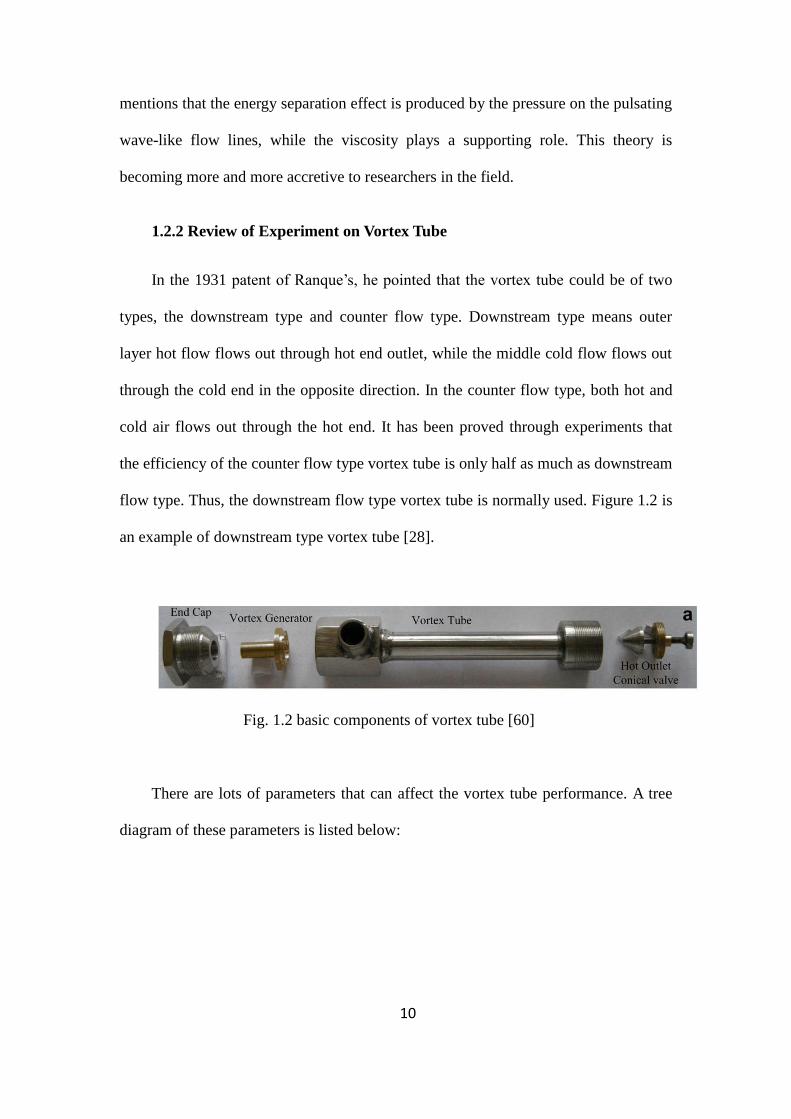
1.2.2 Review of Experiment on Vortex Tube

In the 1931 patent of Ranque’s, he pointed that the vortex tube could be of two

types, the downstream type and counter flow type. Downstream type means outer

layer hot flow flows out through hot end outlet, while the middle cold flow flows out

through the cold end in the opposite direction. In the counter flow type, both hot and

cold air flows out through the hot end. It has been proved through experiments that

the efficiency of the counter flow type vortex tube is only half as much as downstream

flow type. Thus, the downstream flow type vortex tube is normally used. Figure 1.2 is

an example of downstream type vortex tube [28].

Fig. 1.2 basic components of vortex tube [60]

There are lots of parameters that can affect the vortex tube performance. A tree

diagram of these parameters is listed below:

11

Before discussing the influence of different parameters, simple descriptions

about the performance of vortex tube characterizing parameters are listed below:

Refrigeration effect of vortex tube: △ Tc = T0 – Tc ;

Heating effect of vortex tube: △ Th = T0 – Tc ;

Vortex tube cold flow rate ratio:

;

vortex tube unit cooling capacity: q= ·Cp·△ Tc ;

vortex tube refrigeration efficiency: COP=

In the above:

T0 ----- vortex tube inlet temperature, K;

Tc ----- vortex tube cold end temperature, K;

Th ----- vortex tube hot end temperature, K;

p0 ---- vortex tube inlet pressure, Pa;

pc ---- vortex tube cold end pressure, Pa;

ph ---- vortex tube hot end pressure, Pa;

m0 ---- vortex tube inlet mass flow rate, kg/s;

mc ---- vortex tube cold end mass flow rate, kg/s;

12

mh----vortex tube hot end mass flow rate, kg/s;

(1) Operation parameters

inlet pressure p0: Inlet pressure is a key parameter influencing the

performance of vortex tube [31-35]. Most of the articles uses expansion ratio

, defined as the pressure ratio between the inlet and the cold end outlet:

=p0/pc (1.7)

to characterize the inlet pressure effect. In most of experimental studies, the

pressure at the cold end outlet is fixed at the local atmospheric pressure.

There are, however, several works using variable pressure at the cold end

outlet. Studies on the inlet pressure shows that the energy separation effect

increases with the inlet pressure, but levels off to a constant at very high

inlet pressures. Thus, as the inlet pressure is increased higher and higher, the

rate of increases in the pay-off becomes smaller, which may not justify the

use of very high inlet pressure.

inlet temperature T0: there are fewer articles on the inlet temperature effect

because it is not easy to adjust and maintain the inlet temperature. From the

limited number of experiments in the literature and my simulation to be

discussed below, it is shown that the inlet temperature has limited effect on

the vortex tube performance.

(2) Structural parameters

nozzle: this is a very important part of a vortex tube. After an extensive

review of literature, I believe that the structure of nozzle can be

characterized by several aspects:

13

(a) intake: there are helical intake and tangential intake. Takahama and

Parulekar etc believe tangential intake is better than the other type [48-

50].

(b) the form of the nozzle: it means that the cross section of the inlet. The

usual forms include straight nozzle, tapered nozzle. From experimental

data in the literature, which can be found is that, the tapered nozzle

provides a better performance than the other one [35,36,48-50].

(c) cross section of nozzle: the usual shape should be round cross section

and rectangular cross section. Among the two form, rectangular performs

better[35,36,38,42,45,48,51].

(d) number of nozzles: use of different number of nozzles influences the

performance as well. The usual numbers are: 1, 2, 3, 4, 5, 6, 8. Among

them, 4 and 6 is considered to be better [35,36,38,42,45,48,51].

1.2.3 Review of Numerical Simulation on Vortex Tube

Computational Fluid Dynamics is one of the most useful tools for solving

complicated flow problems. Because of the complicated coupled flow and heat

transfer, there is still no well-accepted model or method for numerical simulation in a

vortex tube.

A commonly used turbulence model for vortex tube simulation is Standard k- .

The model was developed as a 2D steady axisymmetric model. The diameter of the

tube is 12mm, the ratio between the tube diameter to length is 10/35, size of cold end

diameters are from 5mm to 7.5mm, numbers of inlet nozzle are 1, 2, 6, nozzle shape

(asymptote type, straight type and round, rectangular). The boundary condition is,

14

inlet pressure 0.5422MPa, and inlet temperature is 300K; cold end outlet pressure is

0.136MPa; hot end pressure is changeable according to flow rate. The results are as

follows: (1) velocity and temperature distribution------along with the rotation velocity

distribution, axial velocity distribution, radial velocity distribution and axial

temperature distribution are computed; (2) six inlet nozzles is found to provide the

best performance. (3) when the cold end outlet diameter is 6mm, the temperature drop

is the largest; (4) the ratio between length and diameter influences the refrigeration

effect limitedly. The tube length to tube diameter ratio has a marginal effect on the

vortex tube performance. Beheral [34] and Alijuwavhel [54] did the same research and

came to the same conclusions.

Bramo [55] employed the standard k- model and ideal gas as working fluid in

the simulation. Three dimensional grid has been used in the vortex tube model by

Exxair company. The results show that the standard k- model is better than RNG k-

model. The standard k- model predicts flow and temperature field more accurately:

the forced vortex occupies the majority of the tube cross-section, and the percentage

of which decreases towards the cold end; energy separation effect happens mainly

near the inlet area of the tube, mainly because of the strong pressure gradient at the

radial and axial direction.

1.3 The Scope of the Current Study

Based on the discussion above, preliminary simulations will be performed for

original vortex tube under the conditions carried out in the experiments reported in the

literature [56]. Variations of the parameters of the vortex tube will then be studied

and compared to the experiments.

15

Simulations will then be performed to optimize the parameters of the original

vortex tube in order to have the best performance of the separation effect.

16

CHAPTER 2

NUMERICAL METHOD, CODE VALIDATION AND VERIFICAION

2.1 Numerical Model for Simulation

Skye [56] believes that in order to understand the complicated flow and heat

transfer phenomenon of the vortex tube, the velocity, pressure and temperature

distributions in the tube needs to be found. The rapid development of computational

fluid dynamics (CFD) provides us a convenient and faster way to study on these

variables in a vortex tube. As discussed above, because of the complexity of the

vortex flow in the tube, choice of a suitable turbulence model is still inconclusive.

Here the standard k- turbulence model is employed since it has a better performance,

as discussed above. The random number generation k- turbulence model and more

advanced turbulence models such as the Reynolds stress equations and RNG k- were

also investigated. However it was found that it is harder to achieve convergence

results for the cases studied here. Nader [58] showed that, because of good agreement

of numerical results with the experimental data, the k- model can be selected to

simulate the effect of turbulence inside of computational domain. Thus, the k- model

will be used in all our simulations.

The mass, momentum, and energy conservation equations are:

( 1 )

( 2 )

( 3 )

17

where the uj is velocity, is density, is viscosity coefficient, is enthalpy and

is the stress tensor component;

In the present study, the ideal gas equation is used:

( 4 )

The kinetic energy(k) of turbulence and (rate of dissipation) are derived from:

( 5 )

( 6 )

In the equations above, Gk, Gb, and YM represent the production of turbulence

kinetic energy according to the average velocity gradients, the generation of

turbulence kinetic energy according to buoyancy, and the contribution of fluctuating

dilatation in compressible turbulence to the overall dissipation rate, respectively.

and are constants. are the turbulent Prandtl number (Pr) for k and . The

turbulent ( or eddy) viscosity, , is computed as:

( 7 )

where is a constant. The model constants will be as:

.

2.2 Geometric Model of Vortex Tube

A picture and schematic of the vortex tube are shown below as Fig. 2.1 and Fig.

2.2. The 10.6 cm working tube length is where the energy separation effect occurs.

Also it will be used as the geometry for the CFD model, which will be described in

the following chapter.

18

Fig. 2.2 vortex tube [60]

The cold and hot exits are axial orifices with areas of 30.2 and 95 mm2,

respectively, as measured with a micrometer. The nozzle of the vortex tube consists of

1 straight slot that direct the flow to high tangential velocities. The parameter values

are listed in the following table.

Fig. 2.3 schematic of vortex tube

19

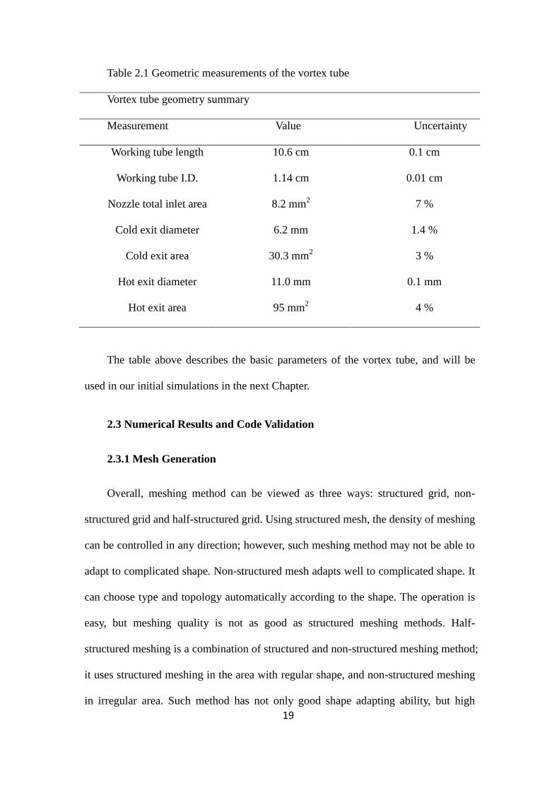
Table 2.1 Geometric measurements of the vortex tube

Vortex tube geometry summary

Measurement Value Uncertainty

Working tube length

Working tube I.D.

Nozzle total inlet area

Cold exit diameter

Cold exit area

Hot exit diameter

Hot exit area

10.6 cm

1.14 cm

8.2 mm2

6.2 mm

30.3 mm2

11.0 mm

95 mm2

0.1 cm

0.01 cm

7 %

1.4 %

3 %

0.1 mm

4 %

The table above describes the basic parameters of the vortex tube, and will be

used in our initial simulations in the next Chapter.

2.3 Numerical Results and Code Validation

2.3.1 Mesh Generation

Overall, meshing method can be viewed as three ways: structured grid, non-

structured grid and half-structured grid. Using structured mesh, the density of meshing

can be controlled in any direction; however, such meshing method may not be able to

adapt to complicated shape. Non-structured mesh adapts well to complicated shape. It

can choose type and topology automatically according to the shape. The operation is

easy, but meshing quality is not as good as structured meshing methods. Half-

structured meshing is a combination of structured and non-structured meshing method;

it uses structured meshing in the area with regular shape, and non-structured meshing

in irregular area. Such method has not only good shape adapting ability, but high

20

meshing quality as well. Normally, numerical computation has the following three

requirements for mesh generation: body-fitted, smooth, reasonable density and good

orthogonality.

By governing equation, control volume integral method, discrete equation,

numerical solution will definitely has some difference to the exact solution, and such

difference is mainly called discretization error. The magnititude discretization error

has some relation to the truncation error. Under the same grid step, discrete error is

getting small along with the increasing rank. To one discrete format, the closer the

mesh is the smaller the error is. However, the close level of the mesh depends on the

computer itself and limit of rounding errors. Generally, the mesh level of numerical

computation satisfies such request: further refinement on the mesh are also employed,

the residual doesn’t change much, thus results can be believed and trusted.

Grid independence analysis is to check the influence to the result according to

the size of the grid. Here one of the representative values in the vortex tube is chosen,

temperature drop, to check whether my grid is good for my simulation.

Fig. 2.4 grid independent check

3 4 5 6 7 8 917

18

19

20

21

22

23

24

25

26

internal size of unit cell(mm)

△Tc

21

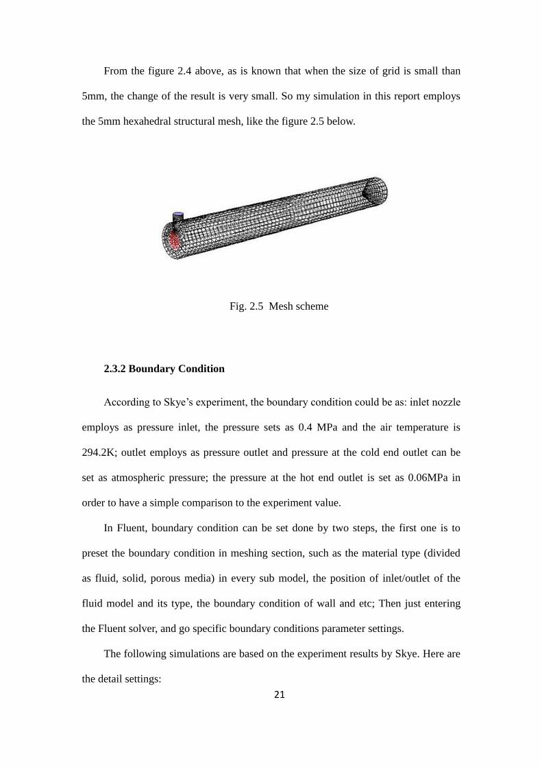
From the figure 2.4 above, as is known that when the size of grid is small than

5mm, the change of the result is very small. So my simulation in this report employs

the 5mm hexahedral structural mesh, like the figure 2.5 below.

Fig. 2.5 Mesh scheme

2.3.2 Boundary Condition

According to Skye’s experiment, the boundary condition could be as: inlet nozzle

employs as pressure inlet, the pressure sets as 0.4 MPa and the air temperature is

294.2K; outlet employs as pressure outlet and pressure at the cold end outlet can be

set as atmospheric pressure; the pressure at the hot end outlet is set as 0.06MPa in

order to have a simple comparison to the experiment value.

In Fluent, boundary condition can be set done by two steps, the first one is to

preset the boundary condition in meshing section, such as the material type (divided

as fluid, solid, porous media) in every sub model, the position of inlet/outlet of the

fluid model and its type, the boundary condition of wall and etc; Then just entering

the Fluent solver, and go specific boundary conditions parameter settings.

The following simulations are based on the experiment results by Skye. Here are

the detail settings:

22

The gas in the vortex tube is set as ideal-gas.

Set the reference pressure to be 101325 Pa, gravity is not considered.

The inlet of vortex tube is set as pressure-inlet, and the pressure is Pin = 4 bar,

and the inlet pressure is Ti = 294.2K.

The cold outlet of vortex tube is set as Pc = 0.1 MPa

The hot outlet of vortex tube is set as Ph = 0.06 MPa

The outside wall of vortex tube is set as stationary wall.

Table 2.2 Basic Boundary Condition

Fluid type Ideal-gas

Inlet pressure 0.4MPa

Inlet temperature 294.2K

Cold outlet pressure 0.1MPa

Hot outlet pressure 0.06MPa

Wall type Stationary wall

The simulation is about three dimensional compressible turbulent flow, and the

coupling of fluid and heat transfer is involved in the computation. Based on these

conditions, the computation methods can be set as following:

Define>models>solver, solver is selected as three dimensional segregated

implicit solver.

Define>models>energy, activate the energy equation.

Define>models>viscous, normally k- turbulent model is employed in

engineering field.

Solve>controls>solution, the diffusive algorithms of governing equation:

pressure option set as standard, pressure-velocity coupling option set as simple

23

algorithms. Momentum, turbulent kinetic energy, turbulent dissipation rate and energy

equation are set as first-order upwind.

Standard of convergence: continuity and the convergence criteria about velocity

on x, y, z three directions is 0.001. The convergence criteria of energy equation is 1e-6.

After finishing the above boundary condition and computation methods settings,

the numerical simulation begins.

First of all, executing initialization, and then opening the monitor of residuals,

and set the convergence standard before the simulation. From the result a

phenomenon can be seen is that after about 30,000 iterations, the residuals of different

variables reach the convergent standard, which is 1e-5.

2.3.3 Simulation Results

Fig. 2.6 vortex tube cross section velocity vector map

From the Fig. 2.6 above, it can be seen clearly that the air in the tube at the

outside zone flow towards the hot end outlet, however, the air in the middle part flow

towards the cold end outlet. The energy separation effect can be approved also by the

24

picture, which is the same to the experiment by Skye.

During the research on vortex tube, it is always expected to know whether the

temperature separation really occurs, and what the temperature could the hot-

outlet/cold-outlet reach. Thus, first of all, the distribution of temperature in the vortex

tube needs to be considered.

In order to have a clear understanding of the temperature distribution and easy to

make a comparison to the experiment, here a map is showed, as the figure 2.7

Fig. 2.7 temperature distribution(contour)

It is delightful to know that, it can be seen that the energy separation in the swirl

chamber clearly from the picture. Because of the interaction between the inner layer

flow and the outer layer flow, the energy inside is decreasing, especially near the

middle part, however, the energy is increasing in the outside. So energy separation

between the middle part of the tube and the out part does exist, and it can be seen

from along the axis peripheral direction, the temperature is increasing. It reaches the

highest at the hot-outlet. The temperature at the middle part of vortex tube is lower

than the peripheral. It decreases along the axis direction and it reaches the lowest at

25

the cold-outlet.

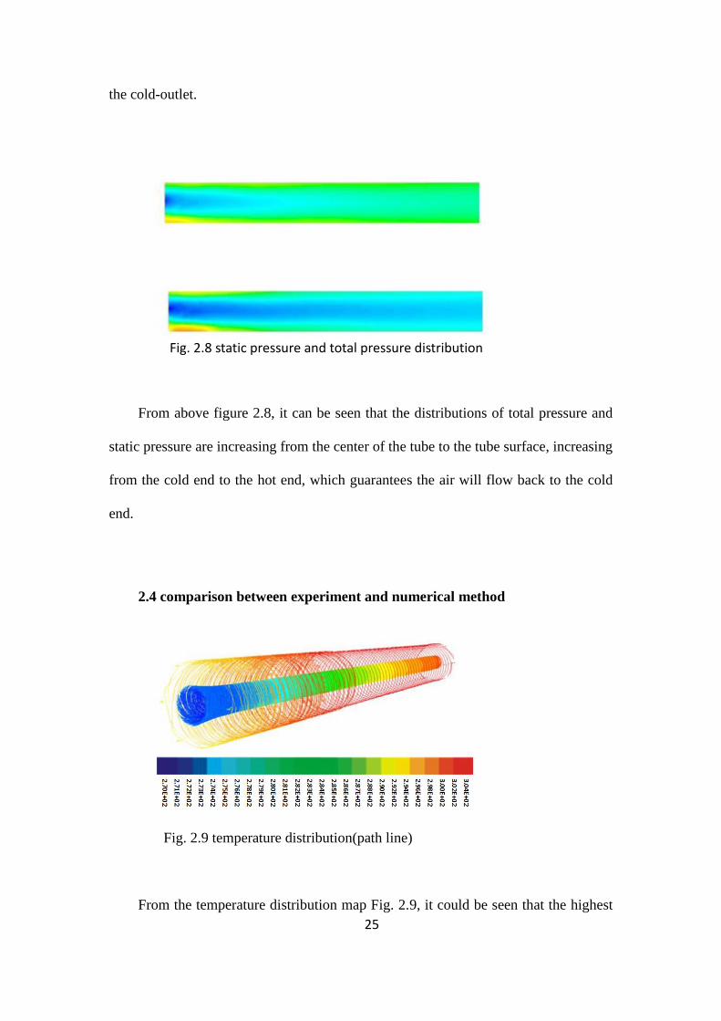
From above figure 2.8, it can be seen that the distributions of total pressure and

static pressure are increasing from the center of the tube to the tube surface, increasing

from the cold end to the hot end, which guarantees the air will flow back to the cold

end.

2.4 comparison between experiment and numerical method

Fig. 2.9 temperature distribution(path line)

From the temperature distribution map Fig. 2.9, it could be seen that the highest

Fig. 2.8 static pressure and total pressure distribution

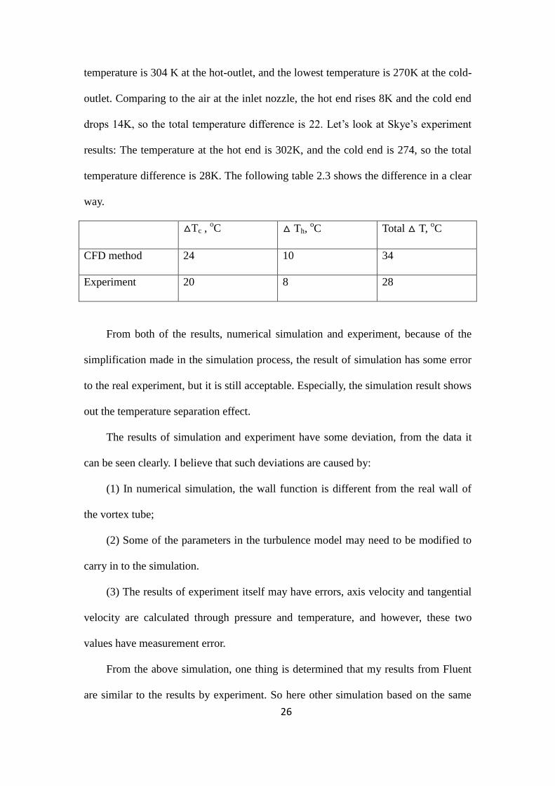
26

temperature is 304 K at the hot-outlet, and the lowest temperature is 270K at the cold-

outlet. Comparing to the air at the inlet nozzle, the hot end rises 8K and the cold end

drops 14K, so the total temperature difference is 22. Let’s look at Skye’s experiment

results: The temperature at the hot end is 302K, and the cold end is 274, so the total

temperature difference is 28K. The following table 2.3 shows the difference in a clear

way.

△Tc , oC △ Th,

oC Total △ T,

oC

CFD method 24 10 34

Experiment 20 8 28

From both of the results, numerical simulation and experiment, because of the

simplification made in the simulation process, the result of simulation has some error

to the real experiment, but it is still acceptable. Especially, the simulation result shows

out the temperature separation effect.

The results of simulation and experiment have some deviation, from the data it

can be seen clearly. I believe that such deviations are caused by:

(1) In numerical simulation, the wall function is different from the real wall of

the vortex tube;

(2) Some of the parameters in the turbulence model may need to be modified to

carry in to the simulation.

(3) The results of experiment itself may have errors, axis velocity and tangential

velocity are calculated through pressure and temperature, and however, these two

values have measurement error.

From the above simulation, one thing is determined that my results from Fluent

are similar to the results by experiment. So here other simulation based on the same

27

turbulence model and process can be carried to find out other good vortex tube

parameters.

28

CHAPTER 3

NEW TUBE DESIGN AND PERFORMANCE EVALUATION

The performance of a vortex tube depends on many parameters as has been

mentioned in Chapter 1. The performances are sensitive to some parameters, while

insensitive to others. The influences of some parameters are not monotonous, and

there should be optimal values that will provide the best result. In this Chapter, a

parametric study is carried on to find out such optimal parameter values.

3.1 The Operation Parameter Analysis

Parameter optimization is carried out by maintaining constant values for all

parameters while varying just a single parameter. In this case, the two important

operation parameters are the inlet temperature and the pressure. The geometry of the

vortex tube analyzed is the one given in the previous chapter.

3.1.1 Vortex Tube Inlet Temperature Optimization Analysis

The figures below show the variation of the inlet temperature on the refrigeration

effect, heating effect and flow-rate of the cold stream exiting the cold end. In these

calculations, the inlet pressure is fixed at 0.4MPa.

29

Fig. 3.1 Effect of inlet temperature on the temperature drop from the cold outlet.

Fig. 3.2 Effect of inlet temperature on the temperature increase from the hot outlet.

Fig. 3.3 Effect of inlet temperature on the flow rate of the cold stream.

Figures 3.1, 3.2, 3.3 show that the influence of the inlet temperature on the

energy separation effect is very small. This is actually good news in some sense, since

270 275 280 285 290 295 300 30522

22.5

23

23.5

24

24.5

25

inlet temperature (K)

△Tc

270 275 280 285 290 295 300 3056

7

8

9

10

11

12

13

inlet temperature (K)

△T

h(K

)

270 275 280 285 290 295 300 3052

2.5

3

3.5

4

inlet temperature (K)

q (

kg/s

)

30

no pre-heating or pre-refrigeration is required to achieve the desired energy separation

effect.

3.1.2 Vortex Tube Inlet Pressure Optimization Analysis

Based on the basic theory of vortex tube, inlet pressure is the key power source

making energy separation works. Thus, parametric study on the inlet pressure effect is

extremely important.

Using the same method as has been done on the inlet nozzle temperature effect,

changing the pressure at the inlet nozzle while keeping other conditions the same. The

inlet temperature is fixed at 294.2K. Fig. 3.4 shows the effect of inlet-pressure/cold-

outlet-pressure ratio on the temperature drop of the cold air stream (refrigeration

effect). As the inlet pressure ratio increases, the expansion ratio of the air goes up,

leading to increased temperature drop at the cold end.

Fig. 3.4 Effect of inlet pressure on the temperature drop at the cold exit.

1 2 3 4 5 6 7 8

16

18

20

22

24

26

28

p0/pc

△Tc (

K)

31

Fig. 3.5 Effect of inlet pressure on temperature rise at the hot exit.

g. 3.6 Effect of inlet pressure on cold stream flow rate.

While not a primary concern, increasing the inlet-pressure/cold-outlet-pressure

ratio also benefits the heating effect, as the temperature rise from the hot end also

increases (Fig. 3.5). The flow rate of the cold air stream also increases with the

pressure ratio (Fig. 3.6).

These results show the benefit of increasing the inlet-to-the-cold-outlet pressure

ratio on both refrigeration and heating. The reason for this increase in the performance

is due to the increased swirling velocity at the inlet from a higher pressure ratio. As

this pressure ratio is increased further, however, the rate of change in the refrigeration

and heating eventually levels off as the air speed near the inlet approaches the speed

1 2 3 4 5 6 7 85

10

15

p0/pc

△T

h(K

)

1 2 3 4 5 6 7 81

2

3

4

5

6

7

8

9

x 10-3

p0/pc

q (

kg/s

)

32

of sound. Ultimately, when shock waves appear at very large inlet-to-outlet-pressure

ratios, the trend actually will be reversed. This dramatic reversal of the pressure ratio

effect will be further analyzed below.

The general results of the influence of inlet pressure and inlet temperature on the

energy separation effect for the original vortex tube should carry over for any vortex

tube. Thus, the general trend will be utilized in the following for designing new vortex

tubes.

3.2 Simple Modification of the Previous Tube

It has been shown that high pressure at the inlet nozzle will improve the

performance of separation effect. In the case of interest to us, however, there are

certain requirements on both the temperature drop and the flow-rate of the cold air

stream. To this end, it can be observed from the Fig. 3.4-3.6, that when the pressure

ratio is 4, the vortex tube can provide a temperature drop of 24 K, and the ratio of the

cold stream flow-rate to inlet flow-rate is one-half.

As mentioned in Chapter 1, our task is to deliver a flow-rate of 40 kg/s with a

cold end exit pressure of 2.5 MPa. Obviously the vortex tube design described in the

previous chapter is not large enough to meet this flow-rate requirement. The most

intuitive way to meet the design objective is to simply enlarge the tube described

proportionally. This approach should be adopted as a starting point for further

optimization by enlarging the original design 10 times geometrically.

Fig. 3.7 shows the temperature distribution along the vortex tube when the inlet

pressure is fixed at 8 MPa and the outlet pressure is fixed at 2.5 MPa. These

preliminary results indicate that there is still room for further improvements in

33

performance.

Fig. 3.7 Vortex tube temperature distribution

There are five ways to improve the design by changing: the size of the inlet; the

size of the outlets (cold, hot); the diameter of the tube; and the length of the tube. The

method adopted here to explore the optimal design is to vary one geometric parameter

while maintaining the rest of four geometric parameters constant.

3.3 Inlet Parameter Optimization

The inlet is the beginning of the whole tube, and it is chosen to be the first. It has

been found that the tangential velocity plays a very important role in the energy

separation effect, and the tangential velocity depends on the shape of the inlet pipe.

The original vortex tube had a circular inlet, and it was later modified to an elliptical

shape by some researchers. It was found that decreasing the minor-to-major semi-axis

ratio, called aspect ratio, increases the tangential velocity, thus enhancing the energy

34

separation effect. Nader [58] mentioned that an aspect ratio of 0.6 delivers a better

result than aspect ratio of one (circular inlet). A rectangular inlet pipe has been

employed with different aspect ratios for the inlet nozzle, similar to the approach of

Upendra [62]. Then the temperature drop at the cold exit can be calculated. These

results are shown in Table 3.1.

Table 3.1 Cold exit temperature drop for different Aspect Ratio of rectangular inlet

(short/long width)

AR △ Tc, oC

0.6 16

0.4 17

0.3 18

0.2 18

From the table above, it is seen that the general trend is that a smaller aspect ratio

provides better cooling performance. As the aspect ratio becomes smaller and smaller,

however, this improvement seems to level off, with the aspect ratio of 0.2 delivering

the best cooling effect.

In addition to the shape of the inlet tube, the cross-sectional area of the inlet tube

is also an important parameter. Yu [57] showed that the (inlet-tube area) to the (the

vortex tube area) ratio (called “nozzle ratio”) affect the performance of the

temperature drop. The effect of different inlet nozzle area on the vortex tube

performance is studied while keeping other parameter fixed, for rectangular inlet with

aspect ratio of 0.2. Five different inlet areas are investigated, with the results

summarized in Table 3.2.

35

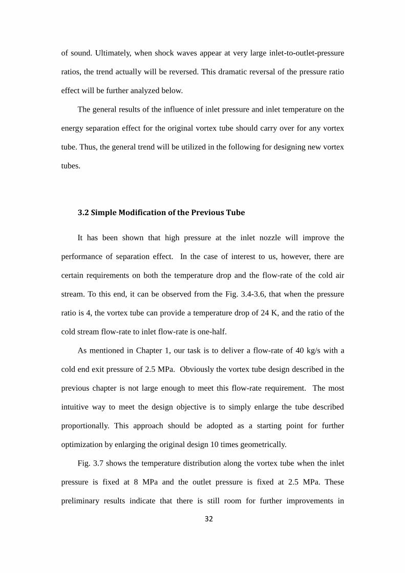
Table 3.2 Effect of inlet area on cold exit temperature drop and flow rate

S (inlet area), mm2 △ Tc,

oC

coldin qq / (inlet-flow-rate/cold-outlet-

flow-rate)

252.2 18 1.7

378.45 20 2.1

756.9 17 2.6

922.5 15 3.0

2000 12 3.5

It is seen from this table, that it is not possible to maximize the cold exit

temperature drop and the cold stream flow-rate for the same choice of the inlet area.

However, this table provides a good reference for other calculations that intends to

perform.

3.4 Vortex Tube Cold end Outlet Optimization

Merculov [59] found that there’s a range of diameter ratio between cold end

outlet orifice to the diameter of the tube, DDc / , between 0.45-0.6, that will optimize

the cold stream temperature drop. This diameter ratio will be extended to 0.45 to 0.75,

with four cold end outlet orifices. Furthermore, while our previous simulation shows

that the inlet to the cold outlet pressure ratio of four provides the best temperature

drop when the radius ratio was one, various inlet-to-cold-outlet pressure ratios will be

considered in our calculations below for diameter ratios DDc / between 0.45 and 0.75.

The basic geometric size of the tube for current research is length(L) equals

1024mm, the diameter of the tube(D) is 57mm, the area of inlet(Sin) is 378.45mm2

36

with the rectangular inlet length h equals 8.7mm and width w=43.5mm, the radius for

the outlet-hot is 25mm. So, the only un-determined geometric parameter is the

diameter of the cold exit orifice. This value can be chosen as an optimization

geometric parameter in the following study.

Now consider a bundle of such tubes. Each of such a tube has the same exit

pressure at the cold exit, which is fixed at 2.5MPa. The number of such tubes in the

bundle, N, is chosen so that the total flow-rate from the cold exit is 40 kg/s. The only

control flow variable is the inlet pressure. Since the flow-rate of the cold stream from

a single tube changes with both the inlet pressure and the cold exit orifice diameter,

the number of tubes required, N, also changes with the inlet pressure and cold exit

orifice diameter.

In Fig. 3.8, the cold-exit-flow-rate vs. the cold exit temperature drop are plotted,

with the inlet pressure and the cold exit orifice diameter as parameters. There are four

curves in Fig. 3.8, each marked with different colors, corresponding to four cold exit

orifice diameter to tube diameter ratios DDc / of 0.45, 0.55, 0.65, 0.75, respectively.

On each of these curves, the cold exit orifice diameter remains the same, the value of

which is indicated in the figure legend, and the inlet pressure, Pin, changes. Thus, the

flow-rate of the cold stream, q, as well as the cold stream temperature drop, △Tc, also

changes along each curve. The number of such tubes required to meet the total cold

stream flow-rate, N, at the data point for the curve are also marked.

For any given cold exit orifice diameter, starting with a small inlet pressure, an

inlet temperature of 294.2K, while keeping the cold exit pressure at 2.5 MPa. Then

gradually increasing the inlet pressure, and compute the cold outlet flow-rate and the

cold outlet temperature. As the inlet pressure is increased, the cold air temperature

37

drops and the inlet flow-rate increases. For example, for 65.0/ DDc (black color

curve), the computation starts with an inlet pressure MPap 50 . What can be found

is that the cold stream temperature is CTc

017 , and 56 tubes (N = 56) are needed to

meet the total cold air flow-rate requirement of 40kg/s. As the inlet pressure is

increased to MPa6 , the cold air temperature increases to CTc

019 , and the N is

dramatically reduced to 32. This trend continues as the inlet pressure is further

increased, and the curve moves in the direction of increased cold air temperature drop

and increased cold air flow-rate (decreased value for N). When the inlet pressure is

increased to MPa8 , however, the cold stream temperature drop reaches its maximum,

with CTc

022 . Beyond this value for the inlet pressure, the cold air temperature

drop starts to decrease, while the flow-rate continues to rise. Thus, for any given cold

exit diameter, there is an optimal inlet pressure that will give the maximum

temperature drop at the cold exit. This optimal inlet pressure actually corresponds to

the critical condition for the inlet air: the inlet air Mach number becomes one at this

inlet pressure. Beyond this inlet pressure, shock waves appear at the inlet, as will be

shown in the next section. Thus, it is preferable to operate in the inlet pressure range

where the inlet air is at subsonic speed.

Similar trends are observed for other exit orifice diameters in Fig. 3.8 for

Dc/D=0.45,0.55,0.65,0.75. It is also observed that there is an optimal choice for the

cold exit orifice diameter as far as the largest temperature drop is concerned:

65.0/ DDc gives the maximum cold air temperature drop, with inlet pressure of

8MPa, and N = 16. This would represent a reasonable design for a bundle of vortex

tube: a C022 temperature drop with 16 tubes to meet the total cold air requirement of

40kg/s, and exit pressure of 2.5MPa.

38

Fig. 3.8 Vortex tube bundle optimization with cold exit orifice diameter and inlet

pressure. The (inlet-pressure, number of tubes) pair, (Pin, N), are marked on each data

point along each curve of the same cold exit orifice diameter.

The trend reversal in the curves in Fig. 3.8 can be understood by plotting the

Mach number distribution along the vortex tube axis. In Fig. 3.9, such plots for

65.0/ DDc and various inlet pressures are shown. The inlet tube is located around

0.005m to 0.05m. For any given inlet pressure, the Mach number near the inlet is

always the highest. When the inlet pressure is less or equal to 8 MPa, the Mach

number along the axis is everywhere below one, indicating subsonic flow in the entire

vortex tube. On the other hand, when the inlet pressure is above 9 MPa, the highest

Mach number is greater than one, which indicates that shock waves will appear near

the inlet. Thus, the reversal in the curves given in Fig. 3.8 corresponds to the

subsonic to supersonic flow transition near the inlet. The temperature distribution

△Tc(oC)

qco

ld (kg/s)

15 16 17 18 19 20 21 220

1

2

3

4

5

6

Dc/D=0.45

Dc/D=0.55

Dc/D=0.65

Dc/D=0.75

(6,49)

(7.5,18)(7.5,15)

(8,13)

(9,12)

(10,14)

(6,23)

(5,56)(5,78)

(5,390)

(5,56)

(6,32) (7.5,23)

(7.5,19)

(9,16)

(8,20)

(8,16)

(10,11)

(12.5,8)(12.5,8)

(9,13)

(12.5,10)(10,9)

(12.5,7)

(15,8)

(10,11)

(8,16)

39

along the tube axis for different inlet pressures plotted in Fig. 3.10 clearly shows the

non-monotonic variation of the exit temperature with the inlet pressure, confirming

the trends shown in Fig. 3.8.

Fig. 3.9 Mach (Ma) number distribution along the tube axis for different inlet

pressures. 65.0/ DDc . The inlet to the is located at x = 0.005m to 0.05m

0 0.2 0.4 0.6 0.8 1 1.20

0.2

0.4

0.6

0.8

1

1.2

1.4

tube position

Mach N

um

ber

Mach Number at different inlet Pressure

inlet pressure 6MPa

inlet pressure 7MPa

inlet pressure 8MPa

inlet pressure 9MPa

inlet pressure 10MPa

(m)

40

Fig. 3.10 Temperature distribution along the tube axis for different inlet pressures,

showing non-monotonic a variant with the inlet pressure, with 65.0/ DDc .

3.5 Hot-end Outlet Optimization

3.5.1 Shape and Angle

The outlet at hot end has a ring shape. In the original vortex tube, it is movable in

order to change the flow rate for different use. However, in our case, it is not that

convenient and not necessary to change such area often. So determine a certain size of

this area is necessary in order to have the best performance. Several angles and shapes

shown in Fig. 3.11 have been used. However, there appears to have no significant

difference in the results.

0 0.2 0.4 0.6 0.8 1 1.2270

275

280

285

290

295

300

tube position

Tem

pera

ture

(K)

Temperature Distribution at Different inlet Pressure

inlet Pressure 6MPa

inlet Pressure 7MPa

inlet Pressure 8MPa

inlet Pressure 9MPa

inlet Pressure 10MPa

(m)

41

Fig. 3.11 The different shape of hot end outlet

3.5.2 The Area of Hot-end Outlet

In addition to the shape and the angle of the hot end valve, the area of the outlet

should also be considered. The results are summarized in Table 3.3.

Table 3.3 Effect of hot outlet radius on temperature drop and flow rate

Rhot , cm c ,oC qin/qcold

23 19 2.2

24 21 2.3

25 22 2.5

26 18 2.8

27 17 3.2

Based on the input value, the inlet pressure is 8MPa and the pressure at the cold

end outlet is 2.5MPa, the values of the radius for the hot end outlet can be determined

42

as 25cm in order to have the best performance.

3.6 Length Of the Tube

Fig. 3.12 Schematic flow pattern of the tube [57]

Fig. 3.12 shows that as the length of the tube increases, the hot end temperature

could be very different. As discussed early, however, the temperature drop of cold air

and flow rate are highly concerned about, not the temperature rise of the hot air. Table

3.4 lists our simulation results for tubes with different length. As seen in this table,

when the tube reaches certain length, the cold air temperature drop no long increases.

A length of 79.8cm gives the largest temperature drop and with the shortest length.

Table 3.4 Temperature drop with different length

L, cm Temperature Drop(△ Tc,oC)

136.8 22

43

125.4 21

102.6 21

91.2 22

79.8 22

68.4 18

57.0 14

3.7 Geometric Optimization Summary

The optimization process conducted in this Chapter leads to the following

optimized set of geometric parameters for a new design of vortex tube that meets our

specified requirement:

Table 3.5 Optimized geometric parameters

Length of the tube 798mm

Diameter of the tube 57mm

Inlet area of the tube 378.45mm2

Inlet Rectangular Aspect ratio 0.2

Inlet nozzle size h=8.7mm w=43.5mm

Radius of hot outlet 25mm

Radius of cold outlet 14.25mm

Fig. 3.13 below provides a mesh scheme with the best geometric value as

mentioned above.

44

Fig. 3.13 Mesh Scheme

45

CHAPTER 4

AIR DRILLING APPLICATION

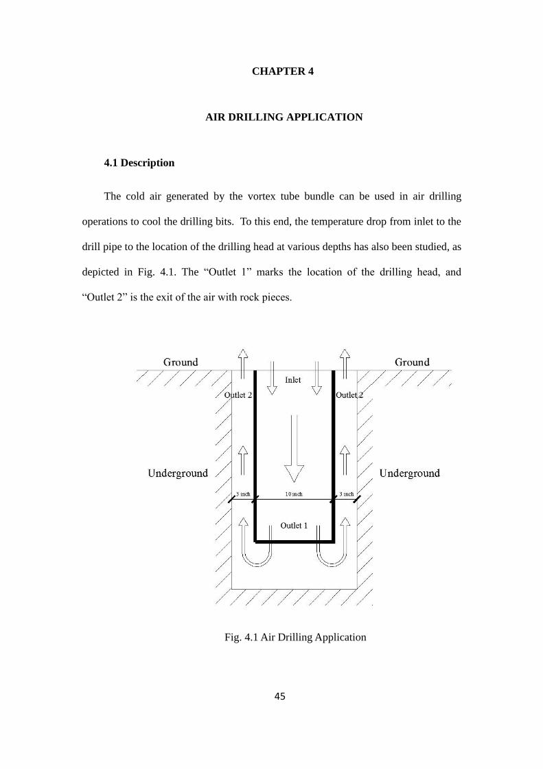
4.1 Description

The cold air generated by the vortex tube bundle can be used in air drilling

operations to cool the drilling bits. To this end, the temperature drop from inlet to the

drill pipe to the location of the drilling head at various depths has also been studied, as

depicted in Fig. 4.1. The “Outlet 1” marks the location of the drilling head, and

“Outlet 2” is the exit of the air with rock pieces.

Fig. 4.1 Air Drilling Application

46

4.2 Boundary Conditions

As has been discussed above, the pressure at cold end outlet of the vortex tube

bundle is 2.5MPa, thus the inlet pressure in the Fig. 4.1 is also 2.5MPa. The drill pipe

is made of steel and the convection heat transfer rate is assumed to be 25 W/m·k-1.

The temperature of the subsurface rock increases approximately 1oC per 33m

increase in depth. The end of drill pipe is set as an interior outlet in the numerical

simulation and the real outlet for the gas is at the ground level which is set to have

the atmospheric pressure. Table 4.1 summarizes the boundary conditions used in the

simulations:

Table 4.1 Boundary condition settings

Inlet-temperature 272 K

Inlet-pressure 2.5MPa

Outlet1 Interior outlet

Outlet2-pressure 0.1MPa

Inner wall material Steel

Outer wall (rock) temperature increase 1 oC/33m

4.3 Meshing

Assumption as the problem is axis-symmetric has been made. To speed up the

computations, the dense mesh near the ends is allocated, and use sparse grids in the

mid portion of the pipe (Fig. 4.2).

47

Fig. 4.2 Mesh method

Grid independence is also conducted, similar to the vortex tube simulations. A

converging plot is given in Fig. 4.3.

Fig 4.3 Convergence study

4.4 Results

Simulations for depths of 100m, 200m and 200m with a rock temperature

48

gradient of 4oC/33m (instead of 1oC/33m), have been performed. Simulations for

depths greater than 500 m require extremely large number of grid points and it takes

significantly longer time to compute. Fig. 4.4 shows the temperature change with

depth in the drill pipe (red line) and the return air along the annulus (black line) for

drilling to 100m. At the drilling head (100 m), the air temperature is 0 oC, an increase

of 2 oC from the cold air entering the drill pipe on the surface.

Fig. 4.4 Drilling to 100m depth.

49

Fig. 4.5 Drilling to 200m depth.

Fig. 4.6 Drilling to 100m depth with 4oC/33m vertical temperature gradient.

Similar calculation for drilling to 200m was also performed, with the

temperature variation with depth given in Fig. 4.5. The air temperature at the drilling

50

head is about 3 oC, an increase of 5oC from the cold air entering the drill pipe on the

surface.

A calculation for a much greater rock temperature gradient, 4oC/33m instead of

1oC/33m, is presented in Fig. 4.6 for drilling to 200 m depth. Even at this large rock

temperature increase rate, the air at drilling head is at a relatively low temperature 5

oC, an increase of 7 oC from the cold air entering the drill pipe on the surface.

These three examples show that the idea of using a vortex tube bundle is

suitable for use in air drilling applications.

51

CHAPTER 5

CONCLUSIONS

A vortex tube can separate a compressible air into a hot and a cold air stream. It

has a simple structure with no moving parts; it is easy to manufacture and assemble,

and it is easy to operate with no maintenance required. Despite of its low energy

efficiency, it has been widely used in many applications.

Using numerical simulations, this thesis explores the possibility of using a vortex

tube bundle for application is drilling applications. The major findings of this study

are:

(1) Inlet pressure is a key parameter for the vortex tube performance. Increasing the

inlet pressure improves the energy separation effect in general. However, when

the inlet pressure to the cold outlet pressure ratio becomes large, the rate of

drop in the cold outlet temperature levels off. Furthermore, when this pressure

ratio exceeds certain value so that shock waves appear, the temperature drop

starts to decreases, corresponding to a transition from subsonic to supersonic

flow at the tube inlet.

(2) An optimization of the temperature drop with geometric parameters has been

performed starting from the original design, and a large scale optimized vortex tube

providing the required performance is found. This optimized vortex tube is

characterized by: Length of 798mm, the diameter of the tube of 57mm, the area of

inlet of 378.45mm2 with rectangular shape of width of 8.7mm and length of 43.5mm;

52

The radius at the hot end outlet of 25mm; and the radius at the cold end outlet of

14.25mm. With this design, the performance of the tube is given in Fig. 3.8 for

various inlet pressures. An inlet air pressure of 8 MPa with 16 such tubes meets the

requirement of the cold end flow-rate of 40kg/s, pressure of 2.5 MPa, with maximum

temperature drop of 22oC.

(3) Simulations using the cold end air from the bundle of vortex tubes for air drilling

application have been performed for drilling depth of 100m, and 200m. The air

temperature at the drilling head can be maintained at 4-5 oC.

53

REFERENCES

[1] G.J. Ranque. Method and apparatus for obtaining from a fluid under pressure two

currents of fluid at different temperatures. United States Patent 1952281, March 27,

1936.

[2] G.J. Ranque. Experiment on expansion in a vortex tube with simultaneous

expansion of hot air and cold air. Le Journal de Physics et Le Radium (Paris),1933,

v.4.1128.

[3] R Hilsch. The use of the expansion of gases ina centrifugal field as cooling

process [J]. The review of scientific instruments, 1947, 8(2): 108-113.

[4] Zhang W.Z. The application of vortex tube in industrial field.

[5] Hu H.T. Air refrigeration cycle characteristics and a new type of refrigeration

equipment research. Energy Saving. 2001(12):13-15.

[6] Sun. G.H. Refrigeration theory and application of vortex tube. 1988

[7] Cao Y. Development and summary of vortex tube research[J]. Cooling

Engineering. 2001(6):1-5.

[8] Huang F.G. Application and practice of vortex tube refrigeration. 1992(3):49-53.

[9] Ding Y.G. Application of vortex tube. Coolin Engineering. 2004(1)

[10] Sha Q.Y. New skill of gas handling. 1994.

[11] Fulton C D. Ranque's tube. ASRE Refrigeration Engineering, 1950, 58(5): 473-

479.

[12] Van Deemter J S. On the theory of the Ranque-Hilsch cool effect. Applied

scientific Research (Series A), 1952,3(3): 174-196.

[13] J E Lay. An experimental and analytical study of vortex-flow temperature

separation by superposition of spiral and axial flows. Transaction of the ASME.

Journal of heat transfer, 1959, 8:213-223.

[14] Stephan K, at el. An investigation of energy separation in a vortex tube.

International Journal of Heat and Mass Transfer, 1983, 36(3): 341-348.

[15] R.G. Deissler and M Perlmutter. Analysis of the flow and energy separation in a

turbulent vortex. International Journal of Heat and Tranfer, 1960: 173-191.

[16] K Stephan, S Lin, M Durst, D Seher. A similarity relation for energy separation in

a vortex tube. International Journal of Heat and Mass Transfer, 1984: 911-920.

54

[17] George W Scheper. Then vortex tube: internal flow date and a heat transfer

theory. Refrigeration engineering, 1951, October: 985-989.

[18] Gulyaev A L. The Ranque effect at low temperatures. International Chemical

Engineering, 1966,6(2):461-466.

[19] T T Cockerill. Thermodynamics and fluid mechanics of Ranque-Hislch vortex

tube:[Mscthesis]. University Cambridge, 1998.

[20] J P Hartnett. Experimental study of the velocity and temperature calibration in a

high velocity vortex tube flow. Transaction of the ASME, 1957, May: 751-758.

[21] C U Linderstrom-Lang. The three-dimensional distributions of tangential

velocity and total-temperature in vortex tube. Journal of Fluid of Mechanics, 1971, 45:

161-187.

[22] Kurosaka M K. Acoustic streaming in swirling flow and the Ranque-Hilsch effect.

Journal of Fluid Mechanics, 1982, 124: 139-172.

[23] E.R.G Eckert. Energy separation in fluid streams. International Communications

in heat and mass transfer, 1989,13(2):127-143.

[24] B Ahlbor, S Groves. Secondary flow in vortex tube. Fluid Dyn. Res, 1997:73-86.

[25] B Ahlborn. The heat pump in a vortex tube. Non-Equilih. Thermodyn, 1998(2):

159-165.

[26] B Ahlborn. The vortex tube as a classic thermodynamics refrigeration cycle.

Journal of Applied Physics, 2000,88(6): 3646-3653.

[27] B Ahlborn, Keller J.U, Staudt R, Treitz G, Rebhan E. Limits of temperature

separation in a vortex tube. Journal of Applied Physics, 1994,27:480-488.

[28] Numerical investigation of gas species and energy separation in the Ranque-

Hilsch vortex tube using real gas model

[29] M.H. Saidi, M.S. Vlipour, Experimental Modeling of Vortex Tube Refrigerator.

Applied Thermal Engineering, 2003,23:1971-1980.

[30] Song. Jiang. Gao et al. experimental research on vortex board refrigeration effect.

Cooling Engineering, 2006, (2).

[31] Hu. Experimental research on small flow rate vortex tube hot end humidification

refrigeration system. Refrigeration Tech. 2002(2).

[32] Heishichiro Takahama. Studies on vortex tube. Japan Society of Mechanical

Engineers, 1965,8(31);

[33] Parulekar B.B Performance of short vortex tubes. Journal of Institution of

55

Engineers(India), 1960(8): 161-164.

[34] Upendra Behera, P.J. Paul, S Kasthuriengan. CFD analysis and experimental

investigations toward optimizing the parameter of Ranque-Hilsch vortex tubee[J].

Heat and mass transfer, 2005.

[35] Metenin V.An investigation into counter-flow vortex tubes. International

Chemical Engineering. 1964,4(3):464-466.

[36] Heishichiro Takahama, Hajime Yokosawa. Energy separation in vortex tubes

with a divergent chamber. Transaction of the ASME Journal of Heat transfer,

1981,103(2):196-203.

[37] Tong Zhou. Turbulent calculation on application of 2nd order Renault stress.

aircraft engine. 1995. (2)

[38] Zhongyue Huang. Improving the refrigeration effect of vortex tube. Refrigeration

Tech, 2002, (1).

[39]Piralishvili S A, Polyaev V M. Flow and Thermodynamics Characteristics of

Energy Separation in a double-circuit Vortex Tube-An Experimental investigation.

Experimental Thermal and Fluid Science, 1996:399-410.

[40] Guillaume D W, Jolly J L.Demonstrating the achievement of lower temperatures

with two-stage vortex tube. Review of Scientific Instrument, 2001:3446-3448.

[41] Arbzov V A, Dubnischev Yu N, Lebrdev A V. Observation of large-scale structure

in vortex tube by colored Foucault-hilbert visualization method. Third International

Conference of Fluid Dynamics Measurement and its Applications. 1997:141-143.

[42] Marlyonvskii V S, Alekseseev V.P. Investigation of the vortex thermal separation

effect for gases vapors. Soviet Physics, 1957,1:2232-2243.

[43] J Marshall. Effect of operation conditions, Physical size and Fluid characteristic

on the gas separation performance of a Linderstrom-Lang vortex tube. Internation

Journal of Heat and Mass Transfer. 1977,20(3):277-231

[44] Ueishichiro Takahama, et al. Performance characteristics of energy separation in

a steam-operation vortex tube. International Journal Engineering Science, 1979,

17:735-744.

[45] Balmer R.T. Pressure Driven Ranque-Hiksch separation in liquids. Journal of

Fluids engineering, 1998, 110:161-164.

[46] R.L. Collins, R.B. Lovelace. Experimental Study of Two-Phase Propane

Expanded through the Ranque-Hilsch vortex tube. Journal of Heat Transfer. ASME,

1979, 101:300-305.

[47] Lancelot A Fekete. Vortex tube separator may solve weight/space limitations.

56

World Oil. 1986:40-44.

[48] A Williams. The cooling of methane with vortex tubes. Journal of Mechanical

Engineering Science, 1971, 13(6):369-375.

[49] Thomas J Bruno. Laboratory application of vortex tube. Journal of Chemical

Education, 1987, 64(11):987-988.

[50] Shou W.D. The application of vortex tube in refrigeration and gas industrial.

1990. (2): 48-51.

[51] Brock Hajdik, Manfred Lorey. Vortex tube can increase liquid hydrocarbon

recovery at plant inlet. Oil and Gas Journal. 1997, 95(36):76-83.

[52] Webster. Analysis of the Hilsch Vortex tube. Refrigerating Engineering.

195:163-171.

[53] He Y.C. Comparison between three kinds of expansion equipment. Cryogenics

and Superconductivity

[54] Aljuwayhel N.F. Nellis G.F. Parametric and internal study of the vortex tube

using a CFD model. International Journal of Refrigeration. 2005,28:442-450.

[55] Bramo, A.R., Pourmahmoud, N., A Numerical Study on The Effect of Length to

Diameter Ratio and Stagnation Point on The Performance of Counter Flow Vortex

Tube, Aust. J. Basic and Appl. Sci., 4(2010), pp. 4943-4957

[56] Skye. Comparison of CFD analysis to empirical data in a commercial vortex tube.

[57] Effects of geometric parameters on the separated air flow temperature of a vortex

tube for design optimization. Energy 37(2012) 154-160.

[58] Nader. Computational Fluid Dynamics Analysis of Helical Nozzles Effects on the

Energy Separation in a Vortex Tube. Thermal Science. 2012, Vol. 16, No. 1, pp. 151-

166

[59] A.P. Merkulov, Vikhrevoi Effekt I Ego Primenenie VTekhnike (Vortex Effect and

Its Application in Technique),Mashinostroenie, Moscow, 1969.

[60] T. Dutta. Numerical investigation of gas species and energy separation in the

Ranque-Hilsch vortex tube using real gas model. International Journal of

Refrigeration 34(2011) 2118-2128.

[61] H.H Bruun. Experimental investigation of the energy separation in vortex

tubes[J]. Journal mechanical engineering science, 1969, 11(6):567-582.

[62] Upendra Behera. CFD analysis and experimental investigations towards

optimizing the parameters of Ranque-Hilsch vortex tube. International Journal of Heat

and Mass Transfer. Volume 48, Issue 10, May 2005, Pages 1961-1973