OPTIMIZATION OF WATER DISTRIBUTION NETWORKS

USING GENETIC ALGORITHM

A THESIS SUBMITTED TO

THE GRADUATE SCHOOL OF NATURAL AND APPLIED SCIENCES

OF

MIDDLE EAST TECHNICAL INIVERSITY

BY

GERÇEK GÜÇ

IN PARTIAL FULFILLMENT OF THE REQUIREMENTS

FOR

THE DEGREE OF MASTER OF SCIENCE

IN

DEPARTMENT OF CIVIL ENGINEERING

APRIL 2006

Approval of the Graduate School of Natural and Applied Sciences

______________________________

Prof. Dr. Canan Özgen Director

I certify that this thesis satisfies all the requirements as a thesis for the degree of

Master of Science.

______________________________

Prof. Dr. Erdal Çokca Head of Department

This is to certify that we have read this thesis and that in our opinion it is fully

adequate, in scope and quality, as a thesis for the degree of Master of Science

______________________________

Assoc. Prof. Dr. Nuri Merzi Supervisor

Examining Committee Members

Prof. Dr. Uygur Şendil (METU, CE)

Prof. Dr. Melih Yanmaz (METU, CE)

Assoc. Prof. Dr. Nuri Merzi (METU, CE)

Assist. Prof. Dr. Ayşe Burcu Altan Sakarya (METU, CE)

Metin Mısırdalı, M.Sc. (Yolsu, CE)

iii

I hereby declare that all information in this document has been obtained and

presented in accordance with academic rules and ethical conduct. I also

declare that, as required by these rules and conduct, I have fully cited and

referenced all material and results that are not original to this work.

Name, Last name : Gerçek GÜÇ

Signature :

iv

ABSTRACT

OPTIMIZATION OF WATER DISTRIBUTION NETWORKS

USING GENETIC ALGORITHM

Güç, Gerçek

Department of Civil Engineering

Supervisor : Assoc. Prof. Dr. Nuri Merzi

April 2006, 76 pages

This study gives a description about the development of a computer model,

RealPipe, which relates genetic algorithm (GA) to the well known problem of

least-cost design of water distribution network.

GA methodology is an evolutionary process, basically imitating evolution process

of nature. GA is essentially an efficient search method basically for nonlinear

optimization cases. The genetic operations take place within the population of

chromosomes. By means of various operators, the genetic knowledge in

chromosomes change continuously and the success of the population progressively

increases as a result of these operations. GA optimization is also well suited for

optimization of water distribution systems, especially large and complex systems.

The primary objective of this study is optimization of a water distribution network

by GA. GA operations are realized on a special program developed by the author

called RealPipe. RealPipe optimizes given water network distribution systems by

considering capital cost of pipes only.

v

Five operators are involved in the program algorithm. These operators are

generation, selection, elitism, crossover and mutation. Optimum population size is

found to be between 30-70 depending on the size of the network (i.e. pipe number)

and number of commercially available pipe size. Elitism rate should be around 10

percent. Mutation rate should be selected around 1-5 percent depending again on

the size of the network. Multipoint crossover and higher rates are advisable. Also

pressure penalty parameters are found to be much important than velocity

parameters. Below pressure penalty parameter is the most important one and

should be roughly 100 times higher than the other.

Two known networks of the literature are examined using RealPipe and expected

results are achieved. N8.3 network which is located in the northern side of Ankara

is the case study. Total cost achieved by RealPipe is 16.74 percent lower than the

cost of the existing network; it should be noted that the solution provided by

RealPipe is hydraulically improved.

Keywords: Water Distribution Systems, Genetic Algorithm, Optimization, Ankara N8 Water Distribution System, Least Cost Design

vi

ÖZ

SU DAĞITIM ŞEBEKELERİNİN

GENETİK ALGORİTMA İLE OPTİMİZASYONU

Güç, Gerçek

İnşaat Mühendisliği Bölümü

Tez yöneticisi : Doç. Dr. Nuri Merzi

Nisan 2006, 76 sayfa

Bu çalışmada RealPipe adlı bilgisayar modelinin geliştirilmesi anlatılmaktadır. Su

şebekelerinde çokca kullanılan en ucuz maliyet tasarımı yöntemi, Genetik

algoritma (GA) yöntemi ile birlikte kullanılarak Ankara N8.3 su şebekesinin

ekonomik çözümü elde edilmiştir.

GA yöntemi doğanın genetik evrimini bilgisayar ortamında taklit eden bir

optimizasyon tekniğidir. GA esas olarak lineer olmayan optimizasyon

durumlarında oldukça etkili bir yöntemdir. Genetik operasyonlar bilgisayar

hafızasında oluşturulan kromozomlar vasıtası ile gerçekleştirilir. Çeşitli operatörler

yardımıyla kromozomlardaki genetik bilgiler her turda sürekli olarak değiştirerek

populasyondaki toplam uygunluğu artırırlar. Bu anlamda GA ile optimizasyon,

şehir şebekeleri dağıtım hatları optimizasyonu için, özellikle kompleks

sistemlerde, çok uygundur. Bu çalışmanın ana amacı şehir şebeke dağıtım

hatlarının genetik algoritma ile optimizasyonudur. Yazar tarafından geliştirilen

RealPipe adlı program GA işlemlerini yapmaktadır. RealPipe, verilen bir şebekeyi

sadece boru fiyatlarını hesaplayarak optimize eder.

vii

Program algoritması beş operatör içermektedir. Bunlar; üretme, seçme, elitizm,

çaprazlama ve mutasyondur. Bu çalışmada genetik algoritma parametreleri de

incelenmiştir. Optimum populasyon büyüklüğü, şebeke ve mevcut boru sayısına

göre değişmekle beraber 30-70 dir. Elitizm oranı yüzde 10 civarında olmalıdır.

Mutasyon oranı şebekeye göre değişmekle beraber, yüzde 1-5 arasında olmalıdır.

Çoklu çaprazlama ve yüksek oranlar önerilmektedir. Aynı zamanda basınç ceza

parametreleri, hız ceza parametrelerinden çok daha önemlidir. Hedef basınç değeri

altı ceza katsayısı en önemli parametredir ve diğerinden 100 kat daha fazla

olmalıdır.

RealPipe ile iki bilinen şebeke incelenmiştir ve beklenen sonuçlara ulaşılmıştır.

Anakara’nın kuzeyinde bulunan N8.3 şebekesi örnek çalışma olarak incelenmiştir.

RealPipe tarafından ulaşılan toplam boru bedeli mevcut şebekeden yüzde 16.74

daha düşük bulunmuştur. Aynı zamanda bu şebeke hidrolik olarak daha verimlidir.

Anahtar Kelimeler: Su Dağıtım Şebekeleri, Genetik Algoritma, Optimizasyon,

Ankara N8 Su Dağıtım Şebekesi, En Ucuz Maliyet Tasarımı

viii

TO MY FAMILY

ix

ACKNOWLEDGMENTS

I would wish to express my deepest gratitude to my supervisor Assoc. Dr. Nuri

Merzi for his valuable guidance, advice, criticism, encouragements and insight

throughout the research.

I also would like to thank my friend Murat Dalkiran and his lovely family who

helped coding the program with a great effort during two years period.

Finally, I would like to thank everybody who has involved in my education since

first grade.

x

TABLE OF CONTENTS

PLAGIARISM ....................................................................................................... iii

ABSTRACT........................................................................................................... iv

ÖZ .......................................................................................................................... vi

DEDICATION .....................................................................................................viii

ACKNOWLEDGEMENTS ................................................................................... ix

TABLE OF CONTENTS........................................................................................ x

LIST OF TABLES ...............................................................................................xiii

LIST OF FIGURES.............................................................................................. xiv

CHAPTERS

1. INTRODUCTION................................................................................................ 1

2. GENETIC ALGORITHM.................................................................................... 3

2.1 – What is Genetic Algorithm ......................................................................... 3

2.2 – Mechanism of Genetic Algorithm............................................................... 3

2.1.1 – Chromosome concept........................................................................... 4

2.1.2. – Generation ........................................................................................... 5

2.1.3 – Selection............................................................................................... 6

2.1.4 – Elitism .................................................................................................. 6

2.1.5 – Crossover.............................................................................................. 6

2.1.6 – Mutation ............................................................................................... 7

2.3 – Implementation of Genetic Algorithm ........................................................ 8

2.4 – Genetic Algorithm in Water Resources .................................................... 10

xi

3. PROGRAM ........................................................................................................ 11

3.1 – EpaNet....................................................................................................... 11

3.1.1 – Introduction of EpaNet....................................................................... 11

3.1.2 – Hydraulic Modeling Capabilities ....................................................... 12

3.1.3 – Water Quality Modeling Capabilities ................................................ 13

3.1.4 – Steps in Using EpaNet ....................................................................... 14

3.1.5 – Hydraulic Simulation Model.............................................................. 15

3.1.6 – Hydraulic Analysis Algorithms.......................................................... 16

3.2 – RealPipe .................................................................................................... 17

3.2.1 – Introduction ........................................................................................ 17

3.2.2 – Penalty Calculations........................................................................... 20

3.2.3 – Hardware Requirements..................................................................... 21

3.2.4 – Software Requirements ...................................................................... 21

3.2.5 – Installation.......................................................................................... 21

3.2.6 – Program Options; Data Input Window............................................... 22

3.2.7 – Running Program ............................................................................... 24

3.2.8. – Reports .............................................................................................. 27

3.3 – Example 1: Shamir Network ..................................................................... 29

3.3.1 – Introduction of the Alperovits and Shamir Network.......................... 29

3.3.2 – EpaNet file derivation ........................................................................ 31

3.3.3 – Determination of Genetic Algorithm Parameters............................... 33

3.3.4 – Solution using RealPipe ..................................................................... 33

3.3.5 –Effects of Parameters of Genetic Algorithm....................................... 36

3.4 – Example 2: Hanoi Network....................................................................... 48

3.4.1 – Introduction of Network..................................................................... 48

3.4.2 – Solution using RealPipe ..................................................................... 51

4. CASE STUDY ................................................................................................... 56

4.1 – Optimization of N8.3 Network ................................................................. 56

4.1.1 – Introduction of Network..................................................................... 56

xii

4.1.2 – Solution using RealPipe ..................................................................... 60

5. CONCLUSION .................................................................................................. 72

5.1 – Summary of the Study............................................................................... 72

5.2 – Conclusion................................................................................................. 72

5.3 – Future Studies............................................................................................ 74

REFERENCES....................................................................................................... 75

xiii

LIST OF TABLES

Table 2.1 Example of Binary Coding...................................................................... 4

Table 2.2 Genetic Algorithm Illustration, Round 1 ................................................ 8

Table 2.3 Genetic Algorithm Illustration, Round 2 ................................................ 9

Table 3.1 Shamir Network, Available Pipe Information ...................................... 30

Table 3.2 Optimum Pipe Results .......................................................................... 35

Table 3.3 Optimum Junction Results .................................................................... 36

Table 3.4 Trial Sets ............................................................................................... 37

Table 3.5 Run Results for Parameter Sets 1.......................................................... 37

Table 3.6 Run Results for Parameter Sets 2.......................................................... 39

Table 3.7 Run Results for Parameter Sets 3.......................................................... 40

Table 3.8 Results Comparison Table for Population Size .................................... 42

Table 3.9 Results Comparison Table for Loop numbers ...................................... 43

Table 3.10 Results Comparison Table for Elitism Rate........................................ 44

Table 3.11 Results Comparison Table for Crossover Rate ................................... 45

Table 3.12 Results Comparison Table for Mutation ............................................. 46

Table 3.13 Results Comparison Table for Pressure Penalty ................................. 47

Table 3.14 Results Comparison Table for Velocity Penalty................................. 48

Table 3.15 Hanoi Network, Available Pipe Information ...................................... 49

Table 3.16 Hanoi Network, Compared Achieved Optimum Pipe Diameters ...... 53

Table 3.17 Hanoi Network, Compared Nodal Pressure Heads ............................. 54

Table 4.1 N8.3 Network Existing Pipe Information ............................................. 56

Table 4.2 N8.3 Network, Existing Node Information........................................... 58

Table 4.3 N8.3 Network, Available Pipe Information .......................................... 60

Table 4.4 Results Comparison Table for Population Size .................................... 62

Table 4.5 N8.3 Network, Pipe Diameters of Selected Optimum Results ............. 63

Table 4.6 N8.3 Network, Pressure Heads of Selected Optimum Results ............. 66

xiv

LIST OF FIGURES

Figure 2.1 Simple Genetic Algorithm Flowchart.................................................... 4

Figure 2.2 Example of Pipe Coding in Binary ........................................................ 5

Figure 2.3 Cross Over Operator .............................................................................. 7

Figure 2.4 Mutation Operator.................................................................................. 7

Figure 3.1 - EpaNet Working Space ..................................................................... 12

Figure 3.2 Overall Optimization Flowchart with RealPipe................................... 17

Figure 3.3 RealPipe Genetic Algorithm Flowchart............................................... 18

Figure 3.4 RealPipe User Interface ....................................................................... 19

Figure 3.5 RealPipe, Available Pipe Information Text......................................... 20

Figure 3.6 Data Input Window.............................................................................. 22

Figure 3.7 Loading Network Information ............................................................. 25

Figure 3.8 Information Window ........................................................................... 25

Figure 3.9 Initial Results Window ........................................................................ 26

Figure 3.10 Progress Window............................................................................... 26

Figure 3.11 Final Results Window........................................................................ 27

Figure 3.12 Report1 Text ...................................................................................... 28

Figure 3.13 Report Exported in to Excel............................................................... 29

Figure 3.14 Shamir Network, Layout.................................................................... 31

Figure 3.15 Shamir Network, Elevations and Pipe Lengths ................................. 32

Figure 3.16 Shamir Network, Velocities and Pressures........................................ 32

Figure 3.17 Shamir Network, Initial Results......................................................... 34

Figure 3.18 Shamir Network, Run Progress ......................................................... 34

Figure 3.19 Shamir Network, Final Results.......................................................... 35

Figure 3.20 Results Comparison Chart for Population Size ................................. 42

Figure 3.21 Results Comparison Chart for Loop numbers ................................... 43

Figure 3.22 Results Comparison Chart for Mutation............................................ 46

Figure 3.23 Hanoi Network, Layout ..................................................................... 50

Figure 3.24 Hanoi Network, Initial Results .......................................................... 51

Figure 3.25 Hanoi Network, Run Progress ........................................................... 52

Figure 3.26 Hanoi Network, Final Results............................................................ 52

xv

Figure 4.1 N8.3 Network, Layout ......................................................................... 59

Figure 4.2 N8.3 Network, Initial Results .............................................................. 61

Figure 4.3 N8.3 Network, Run Progress ............................................................... 61

Figure 4.4 N8.3 Network, Total Cost over Pipe Cost ........................................... 63

Figure 4.5 N8.3 Network, Pressures of Selected Network.................................... 69

Figure 4.6 N8.3 Network, Pipe Diameters of Selected Network .......................... 70

Figure 4.7 N8.3 Network, Velocities of Selected Optimum Network .................. 71

1

CHAPTER 1

1. INTRODUCTION

A water distribution system is an essential infrastructure that conveys water from

the source to the consumers. A typical water distribution system consists of pipes,

pumps, tanks, reservoirs and valves. System is mainly designed considering a

demand pattern, pressure limitations, velocity limitations, quality assurances and

maintenance issues at minimum cost, which can be named as optimal design.

Simulation of hydraulic behavior within a pressurized, looped pipe network is

quite a complex task, which effectively means solving a number of nonlinear

equations. The solution process involves simultaneous consideration of the energy

and continuity equations and the head loss function. Even in a small network of

fifteen pipes, comprising pumps, valves and tanks, there are millions of

combinations for the design depending of commercially available pipe sizes.

Traditionally, the design of water distribution networks has been based on the

designer’s experience. Several trials are run by changing pipe sizes until an

economically feasible solution is reached that meets the design criteria in regard to

the hydraulic conformity. For this kind of applications; designer’s experience,

budget and duration of the design period are very important. Success of the

modeling is mostly governed by these criteria. Because of time limitations, most of

the time, proposed design standards are not fulfilled by a least-cost design. The

construction of a large water distribution system costs too much money; that’s why

designers are looking for various techniques to reach the optimal design for years.

That is where optimization comes into the picture.

Main optimisation techniques are used to get optimal design of a water distribution

system are linear programming, nonlinear programming, and various enumeration

techniques. In this optimization study, problem is defined as minimizing the total

pipe cost, subjected to both pressure and velocity constraints in the presence of

given nodal demands. Since optimization of a water distribution network is rather

2

complicated due to nonlinear relationship between parameters, former

optimization techniques have some disadvantages and difficulties. Some methods

such as enumeration and dynamic analysis (Liang (1971), İnözü (1977), Özer

(1988), Akdoğan (2005)) take too much time for computations and need more

powerful computer. Also a reference book is published by Sevük and Altinbilek

(1977) about computer applications of pipe network.

Recently a new approach to the optimization has been introduced, called genetic

algorithm. Genetic algorithm is a success which is inspired from Darwin’s

evolution theory. It uses the same pattern with the genetic evolution. Main

advantage of the genetic algorithm is simple nature of its algorithm. Detailed

information about optimization techniques will be given in Chapter 2.

The objective of this study is to develop a computer program that optimizes a

water network system using genetic algorithm. Several networks will be examined

using this program and then they will be compared. As a case study, Ankara water

distribution network, pressure zone N8.3 will be examined.

In Chapter 2, a review of optimization techniques of water distribution networks

and genetic algorithm are presented. In Chapter 3, the program and the tools that

the program uses are presented by two sample networks study. In Chapter 4, the

above mentioned case studies are conducted. Finally, conclusions are given in

Chapter 5.

3

CHAPTER 2

2. GENETIC ALGORITHM

2.1 – What is Genetic Algorithm

A Genetic Algorithm is a member of a class of search algorithms based on

artificial evolution (Holland, 1975). Genetic algorithm is the implementation of

Darwin’s evolution theory in optimization applications. In this method, the

variables are presented as numbers on a string called genes and chromosomes

respectively. With the help of some mathematical operations, chromosomes are

evolved during generations according to their fitness’s. The “fitness” evaluation is

based on how well the trial solution meets the “objective function” in terms of

defined goals (i.e. lowest cost or highest reliability) of the optimization. In each

generation, chromosomes with better fitness values survive; on the other hand,

weakest chromosomes are eliminated due to their low fitness’s. Natural selection

ensures that chromosomes with better fitnesses will propagate in the next

populations.

2.2 – Mechanism of Genetic Algorithm

Specific parts of the genetic algorithm which have special function are called

operators. In its simplest form, a genetic algorithm consists of three basic

operators:

• Selection

• Crossover

• Mutation

In addition to these basic operators, Generation operator creates the initial

population of chromosomes. Also, Elitism operator is used in this study which

prevents the loss of successful individual chromosomes. These operators are

4

applied to the current generation to form the next generation. Genetic algorithm

continues until the design criteria have been reached which is defined by the user

at the beginning of the project. Figure 2.1 presents the fundamentals of the genetic

algorithm. At first, the population is evaluated and their fitness’s are determined.

Then, successful individuals are selected and they replaced the unsuccessful ones.

Next step is to form the next population using elitism, crossover and mutation

operators. These processes continue until predefined population number is

reached.

Figure 2.1 – Simple Genetic Algorithm Flowchart

2.1.1 – Chromosome concept

Genetic Algorithm uses chromosome concept to define the variables. Each

decision variable (such as pipe sizes, pump settings, etc.) is defined in genes to

form chromosomes. The common way of encoding is a binary string. A simple

example can be formulated as follows in Table 2.1.

Table 2.1 - Example of Binary Coding

Pipe Size Binary Code 100 mm 00 200 mm 01 300 mm 10 400 mm 11

Breeding Elitism

Crossover Mutation

Evaluation

(fitness)

Population

(t)

Selection

Next Population

(t+1)

5

2.1.2. – Generation

Based on the data assigned in the beginning of the project, the genetic algorithm

will generate an initial population of defined size of population using a random

number generator. Each population is composed of chromosomes. Each solution

(chromosome) will contain randomly generated decision variables. The random

number generator assigns either a 1 or 0 to each bit position in the chromosome

where defined number of bits represents specific decision variables. This operator

is called “Generation” operator. For example, generation operator generates a

population comprising three chromosomes illustrated below in Figure 2.2 with

three chromosomes for ten pipes using coding given above.

Pipe

1

Pipe

2

Pipe

3

Pipe

4

Pipe

5

Pipe

6

Pipe

7

Pipe

8

Pipe

9

Pipe

10

Chrom.1 1 1 0 1 1 1 0 0 0 1 0 1 1 0 0 0 0 1 1 1 400 200 400 100 200 200 300 100 200 400

Chrom.2 0 1 1 1 0 1 1 1 0 0 0 1 0 0 1 1 0 0 0 0 200 400 200 400 100 200 100 400 100 100

Chrom.3 1 0 0 0 1 0 1 1 0 1 1 0 1 0 1 0 1 1 0 1 300 100 300 400 200 300 300 300 400 200

Figure 2.2 - Example of Pipe Coding in Binary

Once the initial population is generated, the Genetic Algorithm will translate each

gene into the corresponding variable (i.e. pipe size) and compute the objective

function (i.e. total cost). Once the objective function is achieved, an analysis will

then be performed for each chromosome of the population and performance

deficiencies will be determined. These deficiencies are defined at the set up stage

of the problem. For example, obtaining an acceptable pressure at the nodes within

defined pressure interval or obtaining an acceptable velocity at the pipes within

defined velocity range will not imply any total cost. On the other hand, genetic

6

algorithm assigns a total cost to each solution (i.e. dollars for each headloss) which

does not satisfy predefined user criteria. A total cost is computed by adding the

pipe cost and related total cost. Genetic algorithm will compute a level of fitness

for each solution in the population based on some function of the total solution

cost. Each individual’s fitness is determined by dividing its penalty value over

total penalty values.

2.1.3 – Selection

This operator is used to eliminate the worst chromosomes due to their low

fitness’s. Once their objective functions are determined at the earlier stage, a

certain number of chromosomes with worst fitness’s are replaced by the same

number of best chromosomes.

2.1.4 – Elitism

Elitism is used to protect the fittest chromosomes from crossover and mutation

operations. The objective is to have some of the best fittest chromosomes as they

are in the next generation and not to loose them. Elitism can rapidly increase the

performance of Genetic Algorithm.

2.1.5 – Crossover

The crossover operator is applied in order to initiate a partial exchange of bits

(information) between parent strings to form two offspring strings. Genetic

Algorithm will randomly pick two solutions for breeding. Total number of

crossover rate is defined by the user at the beginning of the study. Most popular

crossover types are single point, two points and multi points crossovers as shown

in the figures below. Note that all crossover points are randomly selected.

7

Before crossover After crossover

X X X X X X | X X X X X X X X X X | Y Y Y Y Y Y Y Y Y Y | Y Y Y Y

Single point crossover Y Y Y Y Y Y | X X X X

X X X X | X X | X X X X X X X X | Y Y | X X X X Y Y Y Y | Y Y | Y Y Y Y

Two points crossover Y Y Y Y | X X | Y Y Y Y

X X X X X X X X X X X Y X X Y X Y X Y Y Y Y Y Y Y Y Y Y Y Y

Multi points crossover Y X Y Y X Y X Y X X

Figure 2.3 – Cross Over Operator

2.1.6 – Mutation

In order to truly imitate the genetic process, a mutation operator needs to be

incorporated to the random mistakes committed by nature. By occasionally

flipping some of the gene values, the mutation operator allows the introduction of

new features into the pool. In the genetic algorithm process, some alternatives in

the genetic pool may disappear which may lead to the final solution (i.e. all

numbers in a column could be the same). Therefore, introducing the mutation

operator creates the chance to catch these alternatives again.

Pipe

1

Pipe

2

Pipe

3

Pipe

4

Pipe

5

Pipe

6

Pipe

7

Pipe

8

Pipe

9

Pipe

10

1 1 0 1 1 1 0 0 0 1 0 1 1 0 0 0 0 1 1 1Before mutation 400 200 400 100 200 200 300 100 200 400 mutation

1 1 0 1 1 1 0 0 0 1 0 1 1 1 0 0 0 1 1 1After mutation 400 200 400 100 200 200 400 100 200 400

Figure 2.4 – Mutation Operator

8

2.3 – Implementation of Genetic Algorithm

A simple example demonstrating first two steps of simple genetic algorithm will

help to understand the process. Related figures are taken from Goldberg, (1989).

Consider the problem of maximizing the function f(x) = x2, where x is permitted to

vary between 0 and 31. With a five bit (binary digit) unsigned integer we can

obtain numbers between 0 (00000) and 31 (11111). We now simulate a single

generation of a genetic algorithm with reproduction, crossover and mutation. To

start with we select an initial population. We select a population of size 4 by

tossing a fair coin 20 times.

Table 2.2 – Genetic Algorithm Illustration, Round 1

String Id

Initial Population

x Value

f(x)

pselecti

Expected count

Actual count

(Randomly generated)

(Integer) x2 fi / Σf fi / f

1 0 1 1 0 1 13 169 0.14 0.58 1 2 1 1 0 0 0 24 576 0.49 1.97 2 3 0 1 0 0 0 8 64 0.06 0.22 0 4 1 0 0 1 1 19 361 0.31 1.23 1

Sum 1170 1.00 4.00 4 Average 293 0.25 1.00 1 Maximum 576 0.49 1.97 2

We select the mating pool of the next generation by spinning the weighted roulette

wheel four times. Actual simulation of this process using coin tosses has resulted

in string 1 and string 4 receiving one copy in the mating pool, string 2 receiving

two copies, and string 3 receiving no copies as shown in Table 2.2 above.

Comparing actual number of copies with the expected number of copies

(n.pselecti) it is obtained that it should be expected that the fittest chromosomes

gets more copies, the average stays even, and the worst dies off.

9

Table 2.3 – Genetic Algorithm Illustration, Round 2

Mating Pool After

Reproduction

Mate

Crossover Site

New Population

x Value f(x)

(Cross site shown) (Random) (Random) x2 0 1 1 0 | 1 2 4 0 1 1 0 0 12 144 1 1 0 0 | 0 1 4 1 1 0 0 1 25 625 1 1 | 0 0 0 4 2 1 1 0 1 1 27 729 1 0 | 0 1 1 3 2 1 0 0 0 0 16 256

Sum 1754 Average 439 Maximum 729

Having a pool of strings, it is observed that simple crossover proceeds in two

steps: (1) strings are mated randomly, using coin tosses to pair off the couples, and

(2) mated string couples crossover, using coin tosses to select the crossing sites.

Single point crossover is applied in this example. Referring again to Table 2.2,

random choice of mates has selected the second string in the mating pool to be

mated with the first. With a crossing site of 4, the two strings 01101 and 11000

cross and yield two new strings 01100 and 11001. The remaining two strings in the

mating pool are crossed at site 2.

The last operator, mutation, is performed on a bit-by-bit basis. We assume that the

probability of mutation in this test 0,001. With 20 transferred bit position we

should expect 20*0,001 = 0,02 bits to undergo mutation during a given generation.

Simulation of this process indicates that no bits undergo mutation for this

probability value.

Following reproduction, crossover and mutation, the new population is ready to be

tested. To do this, we simply decode the new strings created by the simple genetic

algorithm and calculate the fitness function values from the x values thus decoded.

The population average fitness has improved from 293 to 439 in one generation.

The maximum fitness has increased from 576 to 729 during that same period.

10

Although random processes help cause these happy circumstances, we start to see

that this improvement is not coincidence. The best string of the first generation

(11000) receives two copies because of its high, above-average performance.

When this combines at random with the next highest string (10011) and is crossed

at location 2 (again at random), one of the resulting strings (11011) proves to be a

very good choice indeed.

2.4 – Genetic Algorithm in Water Resources

Many branches could use benefits of Genetic algorithm for optimization problems.

There are several possible areas in the water resources too. Optimization of pipe

diameters (Simpson (1993), Simpson (1994), Simpson (2000), Dandy (1996),

Kahraman (2003), Savic and Walters (1997), Morley (2000)), optimal location for

control valves on a network, optimization of valve control, calibration of water

distribution network, hydraulic management of water distribution system and

optimization of pump run periods could be listed as examples.

11

CHAPTER 3

3. PROGRAM

3.1 – EpaNet

3.1.1 – Introduction of EpaNet

EpaNet is a computer program that performs extended period simulation of

hydraulic and water quality behavior within pressurized pipe networks (Reference

for Epanet). A network consists of pipes, nodes (pipe junctions), pumps, valves

and storage tanks or reservoirs. EpaNet tracks the flow of water in each pipe, the

pressure at each node, the height of water in each tank, and the concentration of

chemical species throughout the network during a simulation period comprised of

multiple time steps. In addition to chemical species, water age and source tracing

can also be simulated.

EpaNet is designed to be a research tool for improving our understanding of the

movement and the fate of drinking water constituents within distribution systems.

It can be used for many different kinds of applications in distribution systems

analysis. Sampling program design, hydraulic model calibration, chlorine residual

analysis, and consumer exposure assessment are some examples. EpaNet can help

assess alternative management strategies for improving water quality throughout a

system. These can include:

• altering source utilization within multiple source systems,

• altering pumping and tank filling/emptying schedules,

• use of satellite treatment, such as re-chlorination at storage tanks,

• targeted pipe cleaning and replacement.

Running under Windows, EpaNet provides an integrated environment for editing

12

network input data, running hydraulic and water quality simulations, and viewing

the results in a variety of formats. These include color-coded network maps, data

tables, time series graphs, and contour plots.

Figure 3.1 - EpaNet Working Space

3.1.2 – Hydraulic Modeling Capabilities

Full-featured and accurate hydraulic modeling is a prerequisite for doing effective

water quality modeling. EpaNet contains a state-of-the-art hydraulic analysis

engine that includes the following capabilities:

• places no limit on the size of the network that can be analyzed

• computes friction headloss using the Hazen-Williams, Darcy-Weisbach, or

Chezy-Manning formulas

13

• includes minor head losses for bends, fittings, etc.

• models constant or variable speed pumps

• computes pumping energy and cost

• models various types of valves including shutoff, check, pressure

regulating, and flow control valves

• allows storage tanks to have any shape (i.e., diameter can vary with height)

• considers multiple demand categories at nodes, each with its own pattern of

time variation

• models pressure-dependent flow issuing from emitters (sprinkler heads)

• can base system operation on both simple tank level or timer controls and

on complex rule-based controls.

3.1.3 – Water Quality Modeling Capabilities

In addition to hydraulic modeling, EpaNet provides the following water quality

modeling capabilities:

• models the movement of a non-reactive tracer material through the network

over time

• models the movement and fate of a reactive material as it grows (e.g., a

disinfection by-product) or decays (e.g., chlorine residual) with time

• models the age of water throughout a network

• tracks the percent of flow from a given node reaching all other nodes over

time

• models reactions both in the bulk flow and at the pipe wall

14

• uses n-th order kinetics to model reactions in the bulk flow

• uses zero or first order kinetics to model reactions at the pipe wall

• accounts for mass transfer limitations when modeling pipe wall reactions

• allows growth or decay reactions to proceed up to a limiting concentration

• employs global reaction rate coefficients that can be modified on a pipe-by-

pipe basis

• allows wall reaction rate coefficients to be correlated to pipe roughness

• allows for time-varying concentration or mass inputs at any location in the

network

• models storage tanks as being either complete mix, plug flow, or two-

compartment reactors.

By employing these features, EpaNet can study such water quality phenomena as:

• blending water from different sources

• age of water throughout a system

• loss of chlorine residuals

• growth of disinfection by-products

• tracking contaminant propagation events.

3.1.4 – Steps in Using EpaNet

One typically carries out the following steps when using EpaNet to model a water

distribution system:

15

1. Draw a network representation of your distribution system or import a basic

description of the network placed in a text file.

2. Edit the properties of the objects that make up the system

3. Describe how the system is operated

4. Select a set of analysis options

5. Run a hydraulic/water quality analysis

6. View the results of the analysis

3.1.5 – Hydraulic Simulation Model

EpaNet’s hydraulic simulation model computes junction heads and link flows for a

fixed set of reservoir levels, tank levels, and water demands over a succession of

points in time. From one time step to the next reservoir levels and junction

demands are updated according to their prescribed time patterns while tank levels

are updated using the current flow solution. The solution for heads and flows at a

particular point in time involves solving simultaneously the conservation of flow

equation for each junction and the headloss relationship across each link in the

network. This process, known as “hydraulically balancing” the network, requires

using an iterative technique to solve the nonlinear equations involved. EpaNet

employs the “Gradient Algorithm” for this purpose. Consult Appendix D for

details. The hydraulic time step used for extended period simulation (EPS) can be

set by the user. A typical value is 1 hour. Shorter time steps than normal will occur

automatically whenever one of the following events occurs:

• the next output reporting time period occurs

• the next time pattern period occurs

• a tank becomes empty or full

16

• a simple control or rule-based control is activated.

3.1.6 – Hydraulic Analysis Algorithms

The method used in EpaNet to solve the flow continuity and head loss equations

that characterize the hydraulic state of the pipe network at a given point in time

can be termed a hybrid node-loop approach. Detailed information on EpaNet

implementation of the hydraulic solution and other information can be found on

the EpaNet manual.

17

3.2 – RealPipe

3.2.1 – Introduction

RealPipe is a water distribution network optimization program. It is written in

Microsoft Visual Basic using genetic optimization algorithm by the author.

RealPipe uses EpaNet, open source module, discussed in the previous chapter for

hydraulic analysis step. Flowchart of running an optimization project is shown

below in Figure 3.2.

Figure 3.2 – Overall Optimization Flowchart with RealPipe

RealPipe’s run algorithm is shown as a flowchart on Figure 3.3 below.

EPANET Create Network

Enter initial network data (Diameter,Length,Demand,Elevation,HWC)

EPANET Export network’s data as INP file

REALPIPE Get network data; INP file

Run the program

START

END

REALPIPE Get genetic algorithm results

18

Figure 3.3 – RealPipe Genetic Algorithm Flowchart

Entry: Genetic Algorithm data, Penalty data, Available Pipe data

Open Epanet project file; Read network data

Run for the initial data for the project file, calculate total network cost

Generation = 1

Generate random population (Generation Operator) (penalty+initial cost) for each member

Make hydraulic analysis (EpaNet) & Calculate total cost

Sort individuals according to the total cost

Store best individual

Generate new population, replacing defined number of best individuals with worst ones (Selection Operator)

Define elite members (Elitism Operator)

Apply cross-over operator to the remaining member

Apply mutation operator to the all population

Make hydraulic analysis (EpaNet) & Calculate total cost

Store best individual

Is generation over?

Generation =

Generation + 1

NO

Write Best solution, Hydraulic analysis results, total cost

YES

END

START

19

RealPipe requires network data prepared by EpaNet to run. At first, any

hydraulically successful network should be defined in EpaNet platform. Then,

objective network’s information data should be exported in the EpaNet’s export

format called INP file with inp extension.

RealPipe has a simple user interface shown in Figure 3.4.

Figure 3.4 – RealPipe User Interface

All network data and data input information are kept on the separate editable text

files. Different network data can be stored separately and user can re-open related

networks data without re-entering each time. Also user can edit, copy, and

duplicate existing data at the windows environment easily. User only uses open

icon in the program to call the related text file in to the program. Loaded

information can be editable also. A sample “available pipe information” data is on

the Figure 3.5.

20

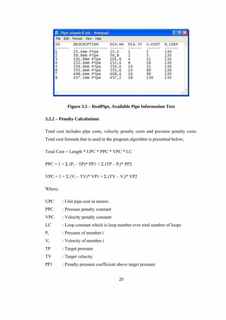
Figure 3.5 – RealPipe, Available Pipe Information Text

3.2.2 – Penalty Calculations

Total cost includes pipe costs, velocity penalty costs and pressure penalty costs.

Total cost formula that is used in the program algorithm is presented below;

Total Cost = Length * UPC * PPC * VPC * LC

PPC = 1 + Σ (Pi – TP)* PP1 + Σ (TP – Pi)* PP2

VPC = 1 + Σ (Vi – TV)* VP1 + Σ (TV – Vi)* VP2

Where;

UPC : Unit pipe cost in meters

PPC : Pressure penalty constant

VPC : Velocity penalty constant

LC : Loop constant which is loop number over total number of loops

Pi : Pressure of member i

Vi : Velocity of member i

TP : Target pressure

TV : Target velocity

PP1 : Penalty pressure coefficient above target pressure

21

PP2 : Penalty pressure coefficient below target pressure

VP1 : Velocity pressure coefficient above target velocity

VP2 : Velocity pressure coefficient below target velocity

In this study, only one target value is used instead of a range composed of two

limitations that are lower and upper boundaries (Savic and Walters (1997)).

Reason for using one target value and two different constraints is to have solutions

as possible as close to the target value. Since there is no upper critical pressure

value in three case studies examined in this thesis, the program doesn’t contain any

upper target value.

3.2.3 – Hardware Requirements

It is recommended that program should be used on an updated computer. Program

doesn’t have any specific hardware constraints. Recommended system is; Pentium

4 2000 mhz or AMD XP+ 2000 mhz, 256mb ram, 100mb empty space on Hard

disk. Similar or higher systems show better performance.

3.2.4 – Software Requirements

Program is designed to use under Windows XP or higher. This doesn’t mean that

program could not run under other operating systems. Compatibility should be

checked by making trial runs.

In order to prepare a network and to see the results of RealPipe, EpaNet software

is needed as it is mentioned previously. EpaNet is a small freeware program and

can be downloaded from the following internet address: www.epa.gov

3.2.5 – Installation

RealPipe has an installation file RealPipe.exe. To install the program execute

installation file under operating system and follow the instructions.

22

3.2.6 – Program Options; Data Input Window

Figure 3.6 – Data Input Window

Load Pipe : Loads “available pipe” information from the

existing, pre-defined text file

Load Network : Opens the exported INP file of the network and

reads the network data from that file that is

necessary for the program to run

Run button : Runs the program with the data exist in the Input

window

Exit button : Exits the program

23

Info Section

Shows general network data after loading network (for information purposes only)

Data Input Section

Genetic trial : Number of genetic run

Population size : Number of population size for each genetic run

Replaced individual number : Number of individuals to be replaced in selection

operation

Loop number : Number of loop for each trial

Elite individual number : Defines the number of elite individuals for elitism

operation

Cross over rate : Defines the rate for cross over operation

Mutation rate : Defines the rate for mutation operation

Target Pressure : Desired target value for pressure in meter

Pressure penalty 1 : Penalty coefficient above target pressure

Pressure penalty 2 : Penalty coefficient below target pressure

Target velocity : Desired target value for velocity in m/sec

Velocity penalty 1 : Penalty coefficient above target velocity

Velocity penalty 2 : Penalty coefficient below target velocity

Generate comparison button : Generate initial and final values in excel

Generate all results button : Generate above report including genetic

algorithm steps

24

Default button : Returns the default values defined in the default

text

Pipe Info Section

Price unit : Selects the price unit (reporting purposes)

Description : Description of the pipe (information purposes)

Diameter mm : Diameter of the pipe in mm (used for calculation)

Diameter inch : Diameter of the pipe in inch (information

purposes)

Unit cost : Unit cost of the pipe per length

Roughness coefficient : Roughness coefficient of the pipe

Update button : Updates changes in the values of selected pipe

Add row button : Ads new pipe information, sorts automatically

Delete row button : Deletes selected pipe information

3.2.7 – Running Program

Using load pipe button, select available pipe information text and click open. Then

using load network button, select inp file that contains network information.

25

Figure 3.7 – Loading Network Information

After having fulfilled these two steps, the program shows network elements in the

info section as shown on Figure 3.8 below.

Figure 3.8 – Information Window

26

At the same time a window, initial results, shows the initial networks hydraulic

solution results with the total cost.

Figure 3.9 – Initial Results Window

At the beginning program reads general information for the data input section from

default.txt file. After making necessary arrangements click on the run button to

start the genetic algorithm operations. Run button can only be active after loading

of pipe and network information. After clicking run button, program starts genetic

algorithm. This operation may take time depending on the network, loop number,

genetic trial number, population size and computer configuration. Progress can be

followed during genetic algorithm operation in the progress window.

Figure 3.10 – Progress Window

27

When the calculations are finished, program opens a new window, final results,

showing the best solution achieved, final networks hydraulic solution results and

the total cost.

Figure 3.11 – Final Results Window

3.2.8. – Reports

Program generates four special reports to examine the genetic algorithm steps and

to make the comparisons. Two text files are automatically generated. First one

includes all generated pipe sizes for all loops called Results1.txt. Second one is

summarized version of the first one. It includes best result of each loop. These

reports can be used to observe the genetic algorithm steps and to determine the

genetic algorithm parameters. Results1.txt report is shown in Figure 3.12 below.

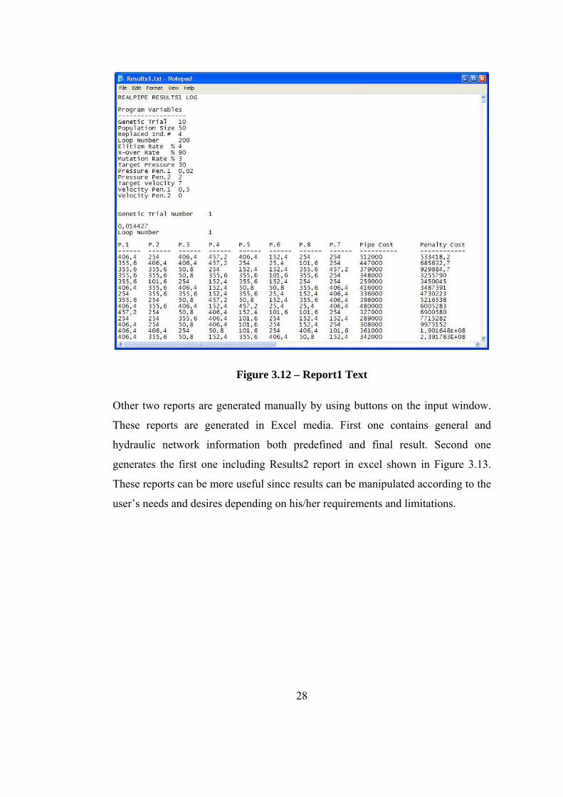
28

Figure 3.12 – Report1 Text

Other two reports are generated manually by using buttons on the input window.

These reports are generated in Excel media. First one contains general and

hydraulic network information both predefined and final result. Second one

generates the first one including Results2 report in excel shown in Figure 3.13.

These reports can be more useful since results can be manipulated according to the

user’s needs and desires depending on his/her requirements and limitations.

29

Figure 3.13 – Report Exported in to Excel

3.3 – Example 1: Shamir Network

Using the program “RealPipe”, two well known networks of the literature have

been examined. First one is the simplest one with 8 pipes and 2 loops. This

network is imaginary and created by Alperovits and Shamir (1977). This network

is widely used earlier for optimization studies. Second one is also widely used, a

famous network called Hanoi Network which is bigger than Shamir Network with

34 pipes. It is a highly skeletonized projection of the water distribution network of

Hanoi city, Vietnam.

3.3.1 – Introduction of the Alperovits and Shamir Network

This network is an imaginary network created by Alperovits and Shamir (1977).

The system has 1 reservoir, 8 pipes and 6 nodes. Each pipe has 1000 m long and

30

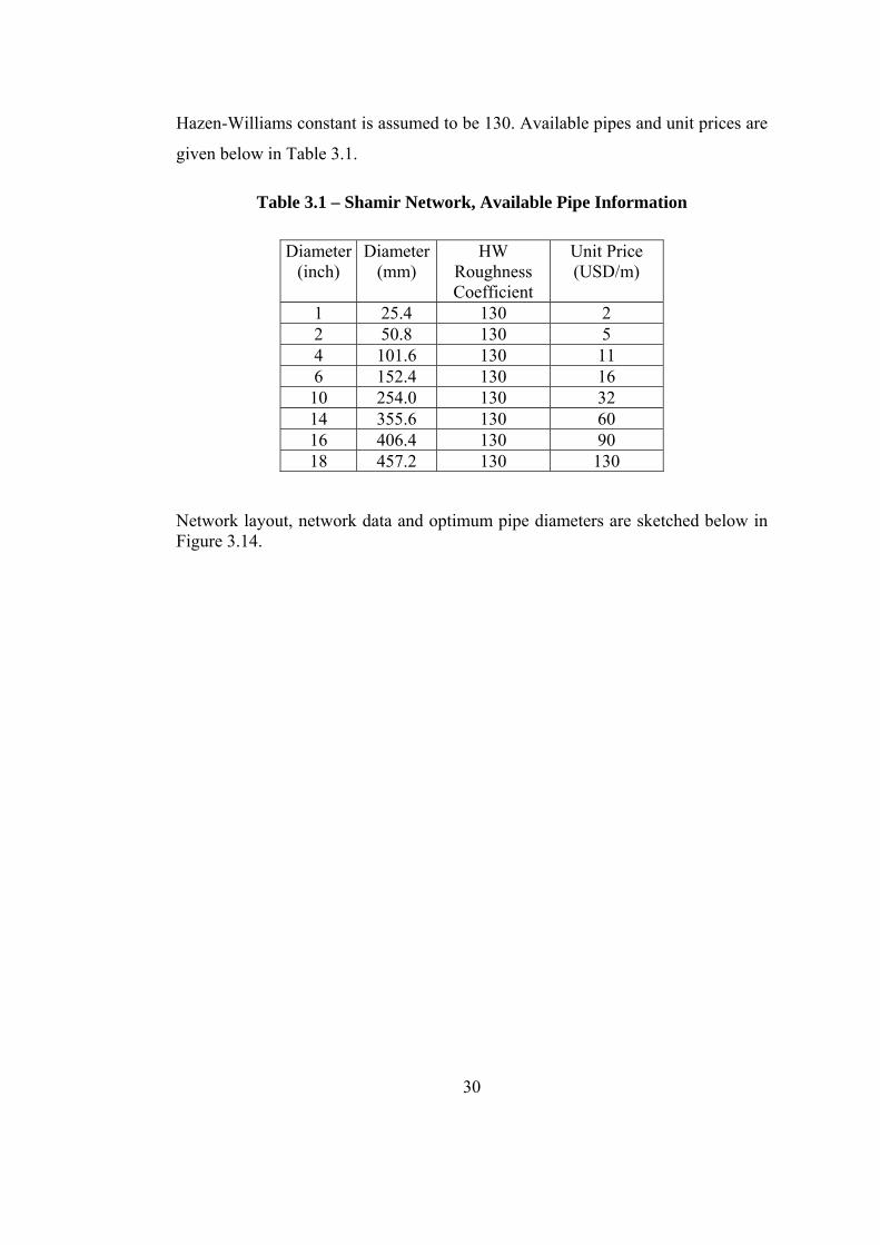
Hazen-Williams constant is assumed to be 130. Available pipes and unit prices are

given below in Table 3.1.

Table 3.1 – Shamir Network, Available Pipe Information

Diameter (inch)

Diameter(mm)

HW Roughness Coefficient

Unit Price (USD/m)

1 25.4 130 2 2 50.8 130 5 4 101.6 130 11 6 152.4 130 16 10 254.0 130 32 14 355.6 130 60 16 406.4 130 90 18 457.2 130 130

Network layout, network data and optimum pipe diameters are sketched below in Figure 3.14.

31

Figure 3.14 – Shamir Network, Layout

3.3.2 – EpaNet file derivation

At first, system is defined in EpaNet. System layout and system elements are

defined in the program. General information like system units, layout properties,

roughness coefficients are assigned. Then length, elevation and demand

information are defined.

Reservoir (210)

1 2 (150) Q=100 [3] D=406.4 L=1000

3 (160) Q=100 [7] D=254 L=1000

5 (150) Q=270 [8] D=25.4 L=1000

4 (155) Q=120 [5] D=406.4 L=1000

7 (160) Q=200

6 (165) Q=330

[1]

D=457.2 L=1000

[2]

D=254 L=1000

[4]

D=101.6 L=1000

(Elevation) [Pipe] Node D=Diameter in mm L=Length in m Q=Demand in m3/hr

[6]

D=254 L=1000

32

Figure 3.15 – Shamir Network, Elevations and Pipe Lengths

As initial diameters, best diameters are assigned having encountered in the

literature. With this best diameter information, best results to achieve are obtained

as shown in Figure 3.16.

Figure 3.16 – Shamir Network, Velocities and Pressures

33

3.3.3 – Determination of Genetic Algorithm Parameters

RealPipe needs basically three elements to run. Available network information

which is inp file, pipe information and genetic algorithm parameters. First two

elements are discussed above. Third element is the key element. It determines the

success and duration of genetic algorithm. It is user dependant. There isn’t known

solution for determining them. It can be determined by trial and error and with the

experience of the user. Different combinations parameters can lead to the solution,

however some can provide quicker response.

3.3.4 – Solution using RealPipe

Several trials have been made using several parameters. Most of the trials, the best

solution is achieved. But one set of parameter is selected as base parameter set

which leads to the result in shortest time period and the most effective way. Base

optimization parameters for this network are given below.

Genetic trial number : 50 Population size : 50 Replaced individual number : 4 Loop number : 40 Elite individual number : 4 Cross over rate : 90% Mutation rate : 3% Target pressure : 30 Pressure penalty above target : 0.02 Pressure penalty below target : 2 Target velocity : 1 Velocity penalty above target : 0.1 Velocity penalty below target : 0.5

34

Figure 3.17 – Shamir Network, Initial Results

Figure 3.18 – Shamir Network, Run Progress

35

Figure 3.19 – Shamir Network, Final Results

In Table 3.2 optimum results achieved by RealPipe compared to the best solution

are presented below.

Table 3.2 – Optimum Pipe Results

Pipe ID

From Node

To Node

Length(m)

Diameter, Initial (mm)

Velocity, Initial (m/s)

Diameter, Final (mm)

Velocity, Final (m/s)

1 7 1 1000 457.2 1.90 457.2 1,90 2 1 2 1000 254.0 1.85 254.0 1,85 3 1 3 1000 406.4 1.46 406.4 1,46 4 3 4 1000 101.6 1.12 101.6 1,12 5 3 5 1000 406.4 1.14 406.4 1,14 6 5 6 1000 254.0 1.10 254.0 1,10 8 4 6 1000 25.4 0.32 25.4 0,32 7 2 4 1000 254.0 1.30 254.0 1,30

Total Cost (USD) 419.000 419.000

When Table 3.2 is examined, the diameters found by RealPipe are the same as the

best result. Also, the computation time to achieve this result is very short which

36

about 3 minutes is. As it is clearly being seen that RealPipe can achieve the best

result, almost every genetic run in very short time. Savic and Walters (1997),

Abebe and Solomatine (1998), Cunha and Sousa (1999), Kahraman (2003) and

Liong and Atiquazzam (2004) are achieved the same result as well.

Table 3.3 – Optimum Junction Results

Junction ID

Elevation (m)

Pressure Head, Initial (m)

Pressure Head, Final (m)

2 150 53.246 53.246 3 160 30.463 30.463 4 155 43.449 43.449 5 150 33.805 33.805 6 165 30.444 30.444 7 160 30.550 30.550

In Table 3.3, it can be seen that there is no pressure less than 30 meters which is

the most important criterion of the program.

3.3.5 –Effects of Parameters of Genetic Algorithm

In this section, alterations in the parameter values and their effects on the genetic

algorithm will be discussed. In order to have a reliable conclusion, 50 trials are

made for each parameter set. Parameters for each set are given below. Alterations

from the base set are marked. 2a is the base set.

37

Table 3.4 – Trial Sets

ID of the set 1a 1b 1c 2a 2b 3 4 5a 5b 6 7a 7b

Population size 50 30 70 50 50 50 50 50 50 50 50 50

Replaced indv. number 4 2 6 4 4 4 4 4 4 4 4 4

Loop number 65 65 65 40 20 40 40 40 40 40 40 40

Elite indv. number 4 4 4 4 4 0 4 4 4 4 4 4

Cross over rate 90% 90% 90% 90% 90% 90% 5% 90% 90% 90% 90% 90%

Mutation rate 3% 3% 3% 3% 3% 3% 3% 0% 30% 3% 3% 3%

Target pressure 30 30 30 30 30 30 30 30 30 30 30 30

Press.pen. above target 0.02 0.02 0.02 0.02 0.02 0.02 0.02 0.02 0.02 0.2 0.02 0.02

Press.pen. below target 2 2 2 2 2 2 2 2 2 1 2 2

Target velocity 1 1 1 1 1 1 1 1 1 1 1 1

Vel.pen. above target 0.1 0.1 0.1 0.1 0.1 0.1 0.1 0.1 0.1 0.1 1 0

Vel.pen. below target 0.5 0.5 0.5 0.5 0.5 0.5 0.5 0.5 0.5 0.5 5 0

Table 3.5 – Run Results for Parameter Sets 1

Trial Number

Pipe Cost

Total Cost

Pipe Cost

Total Cost

Pipe Cost

Total Cost

Pipe Cost

Total Cost

01a Pop=50 Rep=4 01b

Pop=30 Rep=2 01c

Pop=70 Rep=6

02a (Base) Loop=40

1 450,000 731,059 462,000 781,650 419,000 637,517 447,000 679,2672 450,000 747,001 419,000 637,517 420,000 663,240 475,000 761,5063 478,000 817,721 420,000 663,240 419,000 637,517 420,000 663,2404 457,000 772,250 428,000 700,886 419,000 637,517 471,000 783,7805 419,000 637,517 450,000 747,001 419,000 637,517 452,000 737,6436 419,000 637,517 436,000 712,839 466,000 773,037 419,000 637,5177 420,000 663,240 475,000 759,920 445,000 703,418 459,000 748,1978 448,000 739,956 436,000 712,839 419,000 637,517 457,000 772,2509 419,000 637,517 457,000 772,250 420,000 663,240 436,000 712,839

10 475,000 761,506 419,000 637,517 420,000 663,240 477,000 774,54011 420,000 663,240 482,000 767,260 419,000 637,517 419,000 637,51712 420,000 663,240 554,000 843,560 436,000 712,839 466,000 787,76113 450,000 731,059 434,000 698,086 420,000 663,240 450,000 747,00114 478,000 817,721 450,000 731,059 419,000 637,517 457,000 772,250

38

Table 3.5 (continued)

Trial Number

Pipe Cost

Total Cost

Pipe Cost

Total Cost

Pipe Cost

Total Cost

Pipe Cost

Total Cost

15 457,000 772,250 436,000 712,839 419,000 637,517 419,000 637,51716 420,000 663,240 436,000 712,839 450,000 747,001 462,000 770,89617 419,000 637,517 477,000 774,540 419,000 637,517 423,000 669,53518 420,000 663,240 466,000 787,761 462,000 770,896 419,000 637,51719 434,000 698,086 420,000 663,240 462,000 770,896 450,000 715,40720 450,000 731,059 466,000 787,761 450,000 731,059 419,000 637,51721 452,000 737,643 501,000 839,678 419,000 637,517 450,000 731,05922 420,000 663,240 419,000 637,517 420,000 663,240 466,000 767,60123 457,000 772,250 450,000 747,001 420,000 663,240 419,000 637,51724 450,000 731,059 450,000 731,059 450,000 743,040 420,000 663,24025 460,000 777,698 419,000 637,517 420,000 663,240 482,000 794,21726 459,000 701,992 436,000 712,839 450,000 743,040 436,000 712,83927 450,000 731,059 419,000 637,517 445,000 703,418 445,000 703,41828 450,000 743,040 419,000 637,517 450,000 731,059 457,000 772,25029 450,000 731,059 419,000 637,517 450,000 747,001 478,000 789,76430 471,000 783,780 477,000 774,540 462,000 770,896 457,000 772,25031 462,000 770,896 478,000 817,721 420,000 663,240 420,000 663,24032 419,000 637,517 436,000 712,839 420,000 663,240 448,000 715,93133 508,000 769,376 469,000 787,635 445,000 703,418 422,000 641,70834 450,000 731,059 521,000 812,609 436,000 712,839 419,000 637,51735 452,000 737,643 447,000 679,267 419,000 637,517 420,000 663,24036 419,000 637,517 462,000 770,896 419,000 637,517 450,000 715,40737 419,000 637,517 447,000 679,267 420,000 663,240 461,000 719,24638 419,000 637,517 419,000 637,517 420,000 663,240 459,000 741,48939 419,000 637,517 450,000 731,059 436,000 712,839 480,000 786,31540 445,000 703,418 436,000 712,839 457,000 772,250 445,000 703,41841 436,000 712,839 466,000 769,866 419,000 637,517 436,000 712,83942 443,000 717,255 457,000 772,250 445,000 703,418 466,000 773,03743 420,000 663,240 457,000 772,250 457,000 772,250 450,000 715,40744 447,000 679,267 419,000 637,517 482,000 767,260 450,000 747,00145 419,000 637,517 419,000 637,517 450,000 743,040 445,000 703,41846 455,000 747,827 419,000 637,517 434,000 698,086 419,000 637,51747 420,000 663,240 419,000 637,517 420,000 663,240 450,000 715,40748 480,000 801,193 450,000 715,407 419,000 637,517 447,000 679,26749 445,000 703,418 419,000 637,517 420,000 663,240 441,000 704,50650 450,000 743,040 466,000 741,572 450,000 743,040 445,000 703,418

Average 442,980 710,551 447,760 717,958 433,920 690,468 445,600 714,143Minimum 419,000 637,517 419,000 637,517 419,000 637,517 419,000 637,517Maximum 508,000 817,721 554,000 843,560 482,000 773,037 482,000 794,217Std.Dev. 21,339.33 28,693.00 17,484.50 19,442.22 Best sol.# 10 13 14 8

39

Table 3.6 – Run Results for Parameter Sets 2

Trial Number

Pipe Cost

Total Cost

Pipe Cost

Total Cost

Pipe Cost

Total Cost

Pipe Cost Total Cost

02b Loop=20 03 Elitism=0 04 Xover=5 05a Mutation=01 507,000 857,895 484,000 775,808 471,000 770,394 576,000 965,5192 523,000 839,473 450,000 747,001 547,000 840,153 469,000 774,2553 475,000 769,016 459,000 701,992 469,000 787,635 462,000 733,1214 573,000 960,410 497,000 887,259 420,000 663,240 510,000 1,453,3815 467,000 771,485 496,000 840,280 469,000 786,511 526,000 855,3796 534,000 932,454 496,000 800,831 450,000 715,407 569,000 935,9967 455,000 709,972 452,000 806,025 420,000 663,240 461,000 739,5598 508,000 842,142 445,000 799,558 454,000 745,059 666,000 2,150,4989 522,000 788,333 563,000 895,203 450,000 731,059 487,000 873,315

10 451,000 734,637 524,000 891,484 419,000 637,517 608,000 39,746,71211 566,000 933,188 518,000 861,182 467,000 764,042 435,000 587,269,69612 536,000 908,535 536,000 920,465 563,000 883,936 731,000 1,267,14413 436,000 760,071 473,000 751,788 482,000 785,229 580,000 2,100,43914 543,000 910,793 448,000 710,336 419,000 637,517 597,000 1,013,61515 506,000 880,650 457,000 776,219 450,000 743,040 706,000 40,819,86416 556,000 956,144 494,000 807,460 420,000 663,240 439,000 9,312,28717 494,000 814,719 510,000 814,240 419,000 637,517 504,000 847,00718 460,000 777,887 487,000 826,170 419,000 637,517 622,000 10,183,39419 555,000 915,481 478,000 873,138 450,000 743,040 566,000 2,031,39320 483,000 759,908 529,000 903,427 471,000 770,394 480,000 822,62721 529,000 914,633 482,000 785,229 480,000 849,944 617,000 1,314,47522 487,000 741,584 459,000 751,138 478,000 789,764 565,000 1,954,98023 518,000 808,660 494,000 818,049 428,000 700,886 469,000 769,38524 487,000 780,772 508,000 807,876 471,000 770,394 621,000 1,067,53025 507,000 862,077 503,000 826,654 419,000 637,517 509,000 855,81526 553,000 939,157 423,000 669,535 477,000 774,540 522,000 844,94427 436,000 760,071 443,000 803,592 420,000 663,240 422,000 7,329,73428 499,000 875,614 442,000 723,020 438,000 698,802 529,000 858,68029 542,000 901,829 485,000 836,182 457,000 772,250 524,000 877,52930 482,000 814,363 422,000 641,708 419,000 637,517 445,000 703,41831 546,000 954,588 469,000 786,102 422,000 691,977 487,000 1,599,19932 492,000 753,770 466,000 741,572 450,000 731,059 470,000 1,756,70833 554,000 961,928 450,000 715,407 419,000 637,517 576,000 1,031,85634 511,000 817,358 545,000 928,246 419,000 637,517 533,000 3,975,92935 530,000 892,227 469,000 788,261 434,000 698,086 548,000 939,19936 464,000 774,527 487,000 772,972 420,000 663,240 472,000 776,71537 557,000 936,532 448,000 729,166 436,000 712,839 500,000 821,68638 493,000 795,301 518,000 832,871 445,000 703,418 496,000 842,85939 501,000 786,002 469,000 778,018 420,000 663,240 597,000 1,018,06440 543,000 926,470 429,000 681,439 434,000 698,086 541,000 1,608,84341 596,000 1,003,262 557,000 875,674 450,000 715,407 520,000 1,176,25242 541,000 889,817 479,000 780,457 436,000 712,839 540,000 1,115,573

40

Table 3.6 (continued)

Trial Number

Pipe Cost

Total Cost

Pipe Cost

Total Cost

Pipe Cost

Total Cost

Pipe Cost Total Cost

43 473,000 772,425 484,000 775,808 450,000 747,001 402,000 539,584,76844 465,000 903,767 456,000 753,037 419,000 637,517 457,000 772,25045 452,000 731,294 564,000 956,570 423,000 669,535 550,000 939,13346 561,000 957,265 502,000 804,056 450,000 743,040 575,000 1,484,74147 510,000 809,267 464,000 712,881 419,000 637,517 529,000 873,59048 535,000 855,678 452,000 705,079 482,000 767,260 466,000 773,03749 513,000 858,427 478,000 782,256 445,000 703,418 544,000 1,484,98650 469,000 752,261 523,000 853,014 450,000 747,001 543,000 980,075

Average 509,920 847,082 483,320 796,115 446,780 716,361 531,260 25,700,543Minimum 436,000 709,972 422,000 641,708 419,000 637,517 402,000 703,418Maximum 596,000 1,003,262 564,000 956,570 563,000 883,936 731,000 587,269,696Std.Dev. 38,594.62 35,379.83 30,846.75 69,849.93 Best sol.# 0 0 10 0

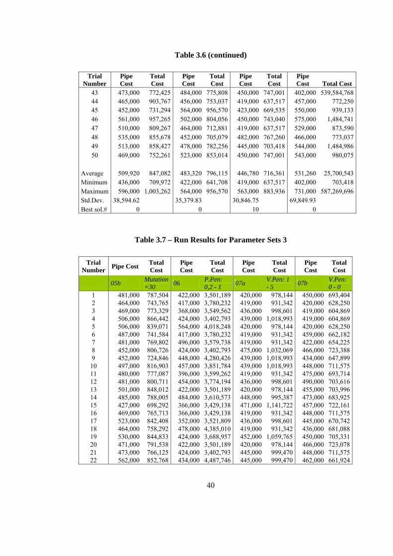
Table 3.7 – Run Results for Parameter Sets 3

Trial Number Pipe Cost Total

Cost Pipe Cost

Total Cost

Pipe Cost

Total Cost

Pipe Cost

Total Cost

05b Mutation =30 06 P.Pen:

0,2 - 1 07a V.Pen: 1 - 5 07b V.Pen:

0 - 0 1 481,000 787,504 422,000 3,501,189 420,000 978,144 450,000 693,4042 464,000 743,765 417,000 3,780,232 419,000 931,342 420,000 628,2503 469,000 773,329 368,000 3,549,562 436,000 998,601 419,000 604,8694 506,000 866,442 424,000 3,402,793 439,000 1,018,993 419,000 604,8695 506,000 839,071 564,000 4,018,248 420,000 978,144 420,000 628,2506 487,000 741,584 417,000 3,780,232 419,000 931,342 459,000 662,1827 481,000 769,802 496,000 3,579,738 419,000 931,342 422,000 654,2258 452,000 806,726 424,000 3,402,793 475,000 1,032,069 466,000 723,3889 452,000 724,846 448,000 4,280,426 439,000 1,018,993 434,000 647,899

10 497,000 816,903 457,000 3,851,784 439,000 1,018,993 448,000 711,57511 480,000 777,087 396,000 3,599,262 419,000 931,342 475,000 693,71412 481,000 800,711 454,000 3,774,194 436,000 998,601 490,000 703,61613 501,000 848,012 422,000 3,501,189 420,000 978,144 455,000 703,99614 485,000 788,005 484,000 3,610,573 448,000 995,387 473,000 683,92515 427,000 698,292 366,000 3,429,138 471,000 1,141,722 457,000 722,16116 469,000 765,713 366,000 3,429,138 419,000 931,342 448,000 711,57517 523,000 842,408 352,000 3,521,809 436,000 998,601 445,000 670,74218 464,000 758,292 478,000 4,385,010 419,000 931,342 436,000 681,08819 530,000 844,833 424,000 3,688,957 452,000 1,059,765 450,000 705,33120 471,000 791,538 422,000 3,501,189 420,000 978,144 466,000 723,07821 473,000 766,125 424,000 3,402,793 445,000 999,470 448,000 711,57522 562,000 852,768 434,000 4,487,746 445,000 999,470 462,000 661,924

41

Table 3.7 (continued)

Trial Number Pipe Cost Total

Cost Pipe Cost

Total Cost

Pipe Cost

Total Cost

Pipe Cost

Total Cost

23 450,000 783,502 422,000 3,501,189 477,000 1,295,353 434,000 647,89924 479,000 801,120 424,000 3,402,793 419,000 931,342 447,000 634,32425 522,000 856,765 422,000 3,501,189 450,000 1,018,241 438,000 668,42726 467,000 773,099 366,000 3,429,138 445,000 997,505 436,000 681,08827 482,000 784,906 426,000 3,842,238 471,000 1,197,871 419,000 604,86928 499,000 845,065 368,000 3,549,562 438,000 972,177 436,000 681,08829 499,000 829,497 450,000 4,474,808 439,000 1,018,993 434,000 647,89930 470,000 785,850 368,000 3,549,562 464,000 1,086,812 445,000 681,79531 503,000 839,018 424,000 3,402,793 436,000 998,601 450,000 670,43432 515,000 859,588 426,000 3,588,295 436,000 998,601 438,000 668,42733 521,000 862,666 424,000 3,402,793 419,000 931,342 419,000 604,86934 478,000 766,784 392,000 4,085,721 469,000 1,065,018 475,000 693,71435 518,000 833,577 466,000 3,609,071 438,000 972,177 447,000 634,32436 477,000 726,253 366,000 3,429,138 450,000 1,122,035 445,000 670,74237 495,000 843,302 399,000 3,637,201 451,000 1,012,719 434,000 647,89938 482,000 781,352 366,000 3,429,138 436,000 998,601 462,000 713,06939 453,000 724,734 352,000 3,521,809 450,000 1,122,035 445,000 670,74240 501,000 853,699 396,000 4,297,234 420,000 978,144 476,000 733,23341 501,000 807,811 457,000 3,851,784 475,000 1,026,720 438,000 668,42742 455,000 733,898 424,000 3,402,793 464,000 1,086,812 450,000 638,85743 450,000 717,805 424,000 3,402,793 448,000 995,387 450,000 693,40444 522,000 844,944 396,000 3,599,262 445,000 997,505 457,000 722,16145 422,000 641,708 424,000 3,402,793 438,000 972,177 447,000 634,32446 487,000 772,972 424,000 3,402,793 439,000 1,005,015 448,000 675,91147 548,000 851,058 426,000 3,588,295 424,000 978,773 466,000 705,87248 557,000 849,160 494,000 3,509,579 436,000 998,601 475,000 693,71449 523,000 863,465 424,000 3,688,957 436,000 998,601 480,000 702,70750 454,000 742,047 454,000 3,590,127 420,000 978,144 419,000 604,869

Average 487,820 795,588 421,260 3,651,417 439,760 1,010,732 447,440 672,534Minim. 422,000 641,708 352,000 3,402,793 419,000 931,342 419,000 604,869Maxim. 562,000 866,442 564,000 4,487,746 477,000 1,295,353 490,000 733,233Std.Dev. 30,508.41 41,316.50 17,410.48 18,119.96 Best sl.# 0 0 8 5

3.3.5.1 – Population Size

Population size is an important part of genetic algorithm process. It is important to

find an optimum number for population size for a specific network which is related

to the number of pipes. It is obvious that large number of population is better but

beyond some point, increasing population does not have the same positive effect

42

on convergence rate. Therefore, it should be large enough to have various numbers

of random individual gene and small enough to make program faster.

In this study Population size 30-replaced individual number 2 (1a), Population size

50-replaced individual number 4 (1b) and Population size 70-replaced individual

number 6 (1c) and are run. Results are as follows.

Table 3.8 – Results Comparison Table for Population Size

Population=30 (01b) Population=50 (01a) Population=70 (01c) Pipe

Cost Total Cost Pipe

Cost Total Cost Pipe

Cost Total Cost

Average 447,760 717,957,57 442,980 710,551,29 433,920 690,467,78 Minimum 419,000 637,516,63 419,000 637,516,63 419,000 637,516,63 Maximum 554,000 843,559,75 508,000 817,721,25 482,000 773,037,06 Std.deviation 28,693.00 21,339.33 17,484.50 Best Solution # 13 10 14

0

100.000

200.000

300.000

400.000

500.000

600.000

700.000

30 50

Population Size

Cost Average Minimum Maximum

Figure 3.20 – Results Comparison Chart for Population Size

Results show that 50 for population are good enough for this network.

43

3.3.5.2 – Loop Number

Loop number is very similar to the previous parameter. Larger number improves

the result but beyond a point it will be useless and extends the run time.

For this case 20, 40 and 65 loop numbers are tested. Results are as follows.

Table 3.9 – Results Comparison Table for Loop numbers

Loop=20 (02b) Loop=40 (02a-base) Loop=65 (01a) Pipe

Cost Total Cost Pipe

Cost Total Cost Pipe

Cost Total Cost

Average 509,920 847,082,28 445,600 714,143,47 442,980 710,551,29 Minimum 436,000 709,971,88 419,000 637,516,63 419,000 637,516,63 Maximum 596,000 1,003,261,63 482,000 794,216,69 508,000 817,721,25 Std.deviation 38,594.62 19,442.22 21,339.33 Best Solution #

0 8 10

0

100.000

200.000

300.000

400.000

500.000

600.000

700.000

20 40 65

Loop Number

Cost Average Minimum Maximum

Figure 3.21 – Results Comparison Chart for Loop numbers

44

As it can be read from the Figure 25, 20 is insufficient for this network and results

stand immature. 40 and 65 reflects almost same results means 65 is unnecessarily

long and lengthen the run time. 40 is good enough to catch the convergence for

this network.

It is no doubt that higher loop numbers may improve some genetic trials. On the

other hand it takes longer times and it is an open end. A stop point should be

selected carefully. Therefore, more trial numbers should be preferred instead of

longer loop numbers.

3.3.5.3 – Elitism

Elitism is introduced in earlier chapters and its importance was already mentioned.

Elitism reserves the best individual for each tour and carries on to the next tour in

order to prevent the probability of losing it. Same network is run without elitism.

Results are presented below in Table 3.10.

Table 3.10 – Results Comparison Table for Elitism Rate

Elite ind.num=4/50 (02a) Elite ind.num=0/50 (03) Pipe Cost Total Cost Pipe Cost Total Cost

Average 445,600 714,143,47 483,320 796,114,65Minimum 419,000 637,516,63 422,000 641,707,94Maximum 482,000 794,216,69 564,000 956,569,50Std.deviation 19,442.22 35,379.83 Best Solution # 8 0

It can clearly be seen that without elitism, program could not achieve the best

result. Each loop best result is subjected to the cross over and mutation. Therefore

it would be impossible to guarantee them to carry for the next round. This trial

shows us the importance of this operator.

45

3.3.5.4 – Crossover

RealPipe uses multipoint crossover as it is mentioned earlier. Larger number of

crossover leads higher ratio of mixing of two individuals which fastens the

convergence. Fourth trial is based on this subject.

Table 3.11 – Results Comparison Table for Crossover Rate

Crossover=90% (02a) Crossover=5% (04) Pipe Cost Total Cost Pipe Cost Total Cost

Average 445,600 714,143,47 446,780 716,360,98Minimum 419,000 637,516,63 419,000 637,516,63Maximum 482,000 794,216,69 563,000 883,935,81Std.deviation 19,442.22 30,846.75 Best Solution # 8 10

Since the network is small, very small percent of crossover can achieve the result

with the help of Elitism and Mutation of course. On the other hand, much greater

standard deviation indicates that genetic algorithm mechanism is not strong

enough with smaller ratio of crossover. On the greater networks, smaller crossover

ratios give results away from the global optimum value.

3.3.5.5 – Mutation

Mutation is another important operator of the Genetic Algorithm. Earlier

researches say that smaller value should be used, i.e. 1-5%. 3% is used in the base

optimization parameter set. Also the sample network is run with 0% and 30%.

Results are shown in Table 3.12.

46

Table 3.12 – Results Comparison Table for Mutation

Mutation=0% (05a) Mutation=3% (02a) Mutation=30% (05b) Pipe

Cost Total Cost Pipe

Cost Total Cost Pipe

Cost Total Cost

Average 531,260 25,700,543.07 445,600 714,143.47 487,820 795,588.02 Minimum 402,000 703,417.94 419,000 637,516.63 422,000 641,707.94 Maximum 731,000 587,269,696 482,000 794,216.69 562,000 866,442.13 Std.deviation 69,849.93 19,442.22 30,508.41 Best Solution # 0 8 0

0

100.000

200.000

300.000

400.000

500.000

600.000

700.000

800.000

0% 3% 30%

Mutation ratio %

Cost Average Minimum Maximum

Figure 3.22 – Results Comparison Chart for Mutation

Without mutation, no goal is achieved. Report created by the program tells that a

better network was found but its total cost is greater than (703,417) the best one

(637,516) which means that its hydraulic properties are away from the desired

limits. Also bigger mutation value could not achieve the result since individuals

are distorted too much during evolution. Another important point is that both

extreme trials have greater variances.

47

3.3.5.6 – Pressure Penalty

Pressure penalty is the most important penalty tool at this study. This penalty

drives the algorithm to converge to the global optimum. Therefore, related two

penalty values must be chosen carefully.

Balance between the above target pressure constant and below target pressure

constant and balance between velocity constants is very critical. Trial runs show

that below target pressure constant should be approximately 100 times bigger than

above one, since it is not desired to have pressure under target pressure. Table 3.13

shows the effects of change in the constants on the results.

Table 3.13 – Results Comparison Table for Pressure Penalty

above=0,02 below=2 (Base,02a) above=0,2 below=1 (06) Pipe Cost Total Cost Pipe Cost Total Cost

Average 445,600 714,143.47 421,260 3,651,416.60 Minimum 419,000 637,516.63 352,000 3,402,792.50 Maximum 482,000 794,216.69 564,000 4,487,745.50 Std.deviation 19,442.22 41,316.50 Best Solution # 8 0

Trial 06 clearly shows that there is no balance between the penalty constants and

program can not be able to understand where the target is. Results for this run are

just numbers.

3.3.5.7 – Velocity Penalty

Velocity penalty can be the named as supporting mechanism. Two different run

are made with different velocity constant as it is shown in Table 3.14.

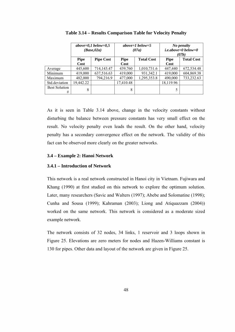
48

Table 3.14 – Results Comparison Table for Velocity Penalty

above=0,1 below=0,5 (Base,02a)

above=1 below=5 (07a)

No penalty i.e.above=0 below=0

(07b) Pipe

Cost Pipe Cost Pipe

Cost Total Cost Pipe

Cost Total Cost

Average 445,600 714,143.47 439,760 1,010,731.6 447,440 672,534.48 Minimum 419,000 637,516.63 419,000 931,342.1 419,000 604,869.38 Maximum 482,000 794,216.9 477,000 1,295,353.8 490,000 733,232.63 Std.deviation 19,442.22 17,410.48 18,119.96 Best Solution

# 8 8 5

As it is seen in Table 3.14 above, change in the velocity constants without

disturbing the balance between pressure constants has very small effect on the

result. No velocity penalty even leads the result. On the other hand, velocity

penalty has a secondary convergence effect on the network. The validity of this

fact can be observed more clearly on the greater networks.

3.4 – Example 2: Hanoi Network

3.4.1 – Introduction of Network

This network is a real network constructed in Hanoi city in Vietnam. Fujiwara and

Khang (1990) at first studied on this network to explore the optimum solution.

Later, many researchers (Savic and Walters (1997); Abebe and Solomatine (1998);

Cunha and Sousa (1999); Kahraman (2003); Liong and Atiquazzam (2004))

worked on the same network. This network is considered as a moderate sized

example network.

The network consists of 32 nodes, 34 links, 1 reservoir and 3 loops shown in

Figure 25. Elevations are zero meters for nodes and Hazen-Williams constant is

130 for pipes. Other data and layout of the network are given in Figure 25.

49

Available pipes and unit prices are given below in Table 3.15 below.

Table 3.15 – Hanoi Network, Available Pipe Information

Diameter (inch)

Diameter(mm)

HW Roughness Coefficient

Unit Price (USD/m)

12 304.8 130 45.73 16 406.4 130 70.40 20 508 130 98.38 24 609.6 130 129.33 30 762 130 180.75 40 1016 130 278.28

50

Figure 3.23 – Hanoi Network, Layout

51

3.4.2 – Solution using RealPipe

Below parameters are used for the optimization of Hanoi network.

Genetic trial number : 10 Population size : 50 Replaced individual number : 4 Loop number : 200 Elite individual number : 4 Cross over rate : 90% Mutation rate : 3% Target pressure : 30 Pressure penalty above target : 0.02 Pressure penalty below target : 2 Target velocity : 7 Velocity penalty above target : 0.5 Velocity penalty below target : 0

Figure 3.24 – Hanoi Network, Initial Results

52

Figure 3.25 – Hanoi Network, Run Progress

Figure 3.26 – Hanoi Network, Final Results

53

Optimum results achieved by RealPipe and comparison to the past studies are

given below in Table 3.16.

Table 3.16 – Hanoi Network, Compared Achieved Optimum Pipe Diameters

Pipe Diameters (inch) Pipe ID

Lengths (m)

Savic and Walters (1997)

Abebe and Solomatine

(1998)

Cunha and Sousa (1999)

Kahraman (2003)

Liong and Atiquazzam

(2004)

Güç (2006)

1 100 40 40 40 40 40 40 2 1350 40 40 40 40 40 40 3 900 40 40 40 40 40 40 4 1150 40 40 40 40 40 40 5 1450 40 30 40 40 40 40 6 450 40 40 40 40 40 40 7 850 40 40 40 40 40 40 8 850 40 30 40 40 30 40 9 800 40 30 40 30 30 40

10 950 30 30 30 30 30 24 11 1200 24 30 24 24 30 24 12 3500 24 30 24 24 24 24 13 800 20 16 20 16 16 12 14 500 16 24 16 12 12 12 15 550 12 30 12 12 12 16 16 2730 12 30 12 16 24 12 17 1750 16 30 16 20 30 20 18 800 20 40 20 24 30 30 19 400 20 40 20 24 30 20 20 2200 40 40 40 40 40 40 21 1500 20 20 20 20 20 20 22 500 12 20 12 12 12 12 23 2650 40 30 40 40 30 40 24 1230 30 16 30 24 30 30 25 1300 30 20 30 24 24 30 26 850 20 12 20 20 12 30 27 300 12 24 12 12 20 20 28 750 12 20 12 16 24 16 29 1500 16 24 16 20 16 16 30 2000 16 30 12 16 16 20 31 1600 12 30 12 16 12 16 32 150 12 30 16 12 16 20 33 860 16 30 16 12 20 16 34 950 20 12 24 20 24 24

Total Cost (Million USD) 6073 7006 6056 6062 6224 6334

54

Shamir network solution was relatively easy to accomplish since it is a small

network. However, in this case, sample space is much larger than the previous one.

Therefore, only one best solution is not expected. Instead, similar results close to

each other are achieved. It is important that observing RealPipe strictly obeys the

minimum pressure rule and all pressure values at the nodes are above 30m. On the

other hand, there are only some nodal pressures under 30m in the other studies that

is highlighted at Table 3.17 below.

Table 3.17 – Hanoi Network, Compared Nodal Pressure Heads

Nodal Pressure Heads (m) Node

ID Savic and Walters (1997)

Abebe and Solomatine

(1998)

Cunha and Sousa (1999)

Kahraman (2003)

Liong and Atiquazzam

(2004) Güç (2006)

1 100 100 100 100 100 100 2 97.14 97.14 97.14 97.14 97.14 97.14 3 61.67 61.67 61.67 61.67 61.67 61.67 4 56.88 58.60 56.87 57.18 57.54 57.54 5 50.94 54.84 50.92 51.61 52.43 52.44 6 44.68 39.51 44.64 45.77 47.13 47.14 7 43.21 38.71 43.16 44.42 45.92 45.93 8 41.45 37.93 41.39 42.84 44.55 44.57 9 40.04 35.72 39.98 41.59 40.27 43.51

10 39.00 34.37 38.93 37.91 37.24 42.77 11 37.44 32.81 37.37 36.35 35.68 38.15 12 34.01 31.65 33.94 32.93 34.52 34.72 13 29.80 30.23 29.74 28.72 30.32 30.51 14 35.13 36.43 35.01 30.68 34.08 30.08 15 33.14 37.24 32.95 27.90 34.08 30.08 16 30.23 37.70 29.87 27.75 36.13 30.59 17 30.32 48.14 30.03 38.57 48.64 44.05 18 43.97 58.63 43.87 50.44 54.00 51.97 19 55.57 60.64 55.54 57.83 59.07 54.00 20 50.44 53.89 50.49 51.28 53.62 49.58 21 41.09 44.54 41.14 41.93 44.27 40.23 22 35.93 44.11 35.97 36.76 39.11 35.07 23 44.21 39.89 44.30 45.75 38.79 42.62 24 38.90 30.62 38.57 34.85 36.37 36.53 25 35.55 30.61 34.86 28.85 33.16 32.52 26 31.53 32.23 30.95 26.58 33.44 31.66 27 30.11 32.71 29.66 26.58 34.38 31.23 28 35.50 33.61 38.66 40.43 32.64 32.62 29 30.75 31.56 29.72 28.93 30.05 30.62

55

Table 3.17 (continued)

Nodal Pressure Heads (m) Node

ID Savic and Walters (1997)

Abebe and Solomatine

(1998)

Cunha and Sousa (1999)

Kahraman (2003)

Liong and Atiquazzam

(2004) Güç (2006)

30 29.73 30.55 29.98 26.17 30.10 30.06 31 30.19 30.50 30.26 26.16 30.35 30.09 32 31.44 30.28 32.72 26.41 31.09 30.98

In the light of Table 3.17 above, it is observed that solution with lowest cost is

achieved by Cunha and Sousa (1999), however this solution could not meet the

pressure constraint at five nodes. The solution with the highest cost is achieved by

Abebe and Solomatine (1998). This solution meets all the constraints.

Also, it can be concluded that RealPipe can find solutions that is between the past

studies. Moreover RealPipe’s solution has no constraint defect. It should be

pointed that only 10 trials had performed. More trials should have performed to

obtain a better solution.

56

CHAPTER 4

4. CASE STUDY

Genetic algorithm program developed for this study called RealPipe has already

been introduced and two sample networks have then been studied using this

program. In this chapter, as a case study, a skeletonized model of an existing

network (N8.3) of Ankara water distribution system is examined (Merzi et al.

1998a, 1998b). N8.3 is located at the end of the North main pressure zone of the

city. The pressure zone N8.3 comprises the districts Çiğdemtepe, Sancaktepe,

Şehit Kubilay and Yayla (Yenimahalle and Keçiören counties). There are about

25000 people living there with lower incomes. This is the largest network

examined in this study with 83 pipes and 60 nodes.

4.1 – Optimization of N8.3 Network

4.1.1 – Introduction of Network

This network is a skeletonized model of the pressure zone N8.3 of northern

Ankara. It has 83 pipes, 60 nodes and 2 reservoirs. Pump is not introduced in this

model in order to simplify the network; a reservoir has been placed instead of

existing pump (P23). Network link information of the existing system is given in

Table 4.1 below.

Table 4.1 – N8.3 Network Existing Pipe Information

Pipe Id Length (m)

Diameter (mm) Pipe Id Length

(m) Diameter

(mm) 82015 46 150 85008 273,6 150 82009 56 150 85014 122,4 100 82014 268 150 85015 181 125 82024 27 100 85016 136 200 82023 65 250 85017 272 125 82021 115 200 85019 292 150 82026 356 150 84001 479,4 100 83001 258 100 84002 178 200 83002 180 100 84003 161 100

57

Table 4.1 (continued)

Pipe Id Length (m)

Diameter (mm) Pipe Id Length

(m) Diameter

(mm) 83021 213,5 250 84005 140 150 83018 52 125 84006 191 125 83013 70 100 84009 349 150 83015 109 125 84010 294 200 83017 28 125 83003 159,5 150 83008 136 100 83005 282 250 83006 76 100 83009 181 150 85024 59 150 83010 453 150 84007 116 100 83012 561 250 84008 268 150 83016 136 125 85018 183 200 83019 440,5 125 85013 55 125 83020 528,5 150 85021 58 200 82002 449 250 85012 108 200 82003 184 250 85011 114 200 82004 401 150 85022 23 100 82005 270 100 M24 175 500 82006 252 150

83011 402 125 82007 104 200 83007 5 125 82008 181 150 83014 5,1 100 82010 267 150 84012 29,3 150 82011 304 125 84011 13,5 150 82013 323 100 85020 7,6 150 82012 203,5 200 83004 41 250 82018 170 200 85023 18 100 82019 284 200 82001 15 250 82020 652 125 84004 23 150 82022 69 200 85001 100 100 82025 101 100 85002 161 100 80027 386 200 85003 196 100 M23 999,99 500 85004 103 200 M9 306,6 500 85005 135 200 M1 424,1 500 85007 521 150

Nodal demand data were obtained after having examined the daily demand curve

of August 16, 2001, at which one of the highest water usages of the year occurs.

Nodal demands of the related peak hour values of that day are presented on Table

4.2. Network layout is given on Figure 31 as well.

58

Table 4.2 – N8.3 Network, Existing Node Information

Node Id Elevation Demand (lt/s) Node Id Elevation Demand

(lt/s) 100 1130.65 0.681448 783 1102.07 0.787211 103 1121.22 1.760420 784 1103.6 2.016490 109 1093.83 0.452250 785 1107.49 1.134420 113 1128.25 1.558580 790 1081.46 3.931400 122 1113.44 2.102530 794 1118.86 1.060320 133 1096.15 1.021000 799 1078.28 0.924975 138 1083.85 1.509020 801 1116.19 0.699398 160 1121.51 0.825735 802 1115.64 1.013580 411 1117.74 2.150740 813 1103.82 0.632420 416 1120.65 0.191525 817 1097.32 1.827250 419 1127.29 1.895270 819 1108.57 1.090780 420 1099.27 1.194620 820 1107.13 0.841508 575 1099.91 0.680308 822 1096.42 0.190796 578 1120.68 0.620925 823 1095.11 0.329633 580 1124.97 0.815858 1910 1082.93 2.816240 587 1118.99 0.838415 3078 1098.98 1.809030 588 1133.48 0.565602 3144 1112.1 1.148520 589 1079.97 1.244130 3147 1121.36 0.581499 591 1071.41 1.503890 3209 1096.29 4.684320 595 1083.36 1.286100 3212 1097.05 0.082779 607 1093.23 1.646500 3213 1071.26 0.888419 612 1076.44 0.947418 3221 1105.05 0.548160 618 1101.7 0.659789 3222 1104.91 0.095903 624 1114.46 0.299486 3286 1115.21 0.543169 628 1089.6 0.284781 3299 1096.87 0.101758 629 1089.8 0.790042 3300 1095.67 0.041481 631 1114.77 0.692856 AN23 1151.66 0.000000 771 1103.82 0.947974 AN24 1051.32 0.000000 774 1117.1 0.875683 511 1096.42 4.283320 780 1108.65 1.833420 3285 1103.32 0.723867 782 1098.99 0.706399 3830 1079.02 0.710366

59

Figure 4.1 – N8.3 Network, Layout

60

Hazen-Williams coefficient is taken 130 for each pipe. Eleven commercially

available ductile iron pipes are used for the solution whose unit prices are taken

from Keleş (2006). Pipe diameters and unit prices are given below in Table 4.3.

Table 4.3 – N8.3 Network, Available Pipe Information

Diameter(mm)

Roughness Coefficient

Unit Price (USD/m)

100 130 16.19 125 130 17.51 150 130 19.04 200 130 24.98 250 130 31.43 300 130 37.86 350 130 45.96 400 130 51.78 450 130 65.88 500 130 71.27 600 130 93.57

4.1.2 – Solution using RealPipe

Below parameters are used for the optimization of N8.3 network.

Genetic trial number : 20 Population size : 50 Replaced individual number : 4 Loop number : 300 Elite individual number : 4 Cross over rate : 90% Mutation rate : 3% Target pressure : 30 Pressure penalty above target : 0.02 Pressure penalty below target : 2 Target velocity : 7 Velocity penalty above target : 0.5 Velocity penalty below target : 0

61

Figure 4.2 – N8.3 Network, Initial Results

Figure 4.3 – N8.3 Network, Run Progress

20 trials have been accomplished; obtained total pipe costs and total total costs are

tabulated below in Table 4.4.

62

Table 4.4 – Results Comparison Table for Population Size

Trial No Pipe Cost(YTL)

Total Cost (YTL)

17 375,884 2,325,425 8 383,316 2,376,106 13 386,255 2,347,722 14 389,274 2,367,675 2 389,662 2,391,751 10 396,542 2,371,988 4 408,313 2,385,053 5 418,978 2,377,690 20 453,371 2,131,344 11 457,592 2,180,971 9 460,108 2,157,317 3 463,271 2,012,622 1 464,899 2,133,176 18 467,879 2,135,391 16 468,391 2,052,304 12 474,716 2,002,782 6 477,225 2,050,423 7 485,942 2,095,401 15 491,359 2,146,285 19 496,573 2,127,289

In the light of results tabulated above, it was founded that total pipe costs of some

solutions are cheaper than the cost of the existing system that is 451,475 YTL. On

the other hand, there are solutions with lower total costs than the cheapest solution.

Since all velocities are within the defined range, there is no velocity penalty in the

total costs.

Total pipe cost over total cost graph is presented below in order to compare results

with a linear trendline showing the relation on Figure 4.4.

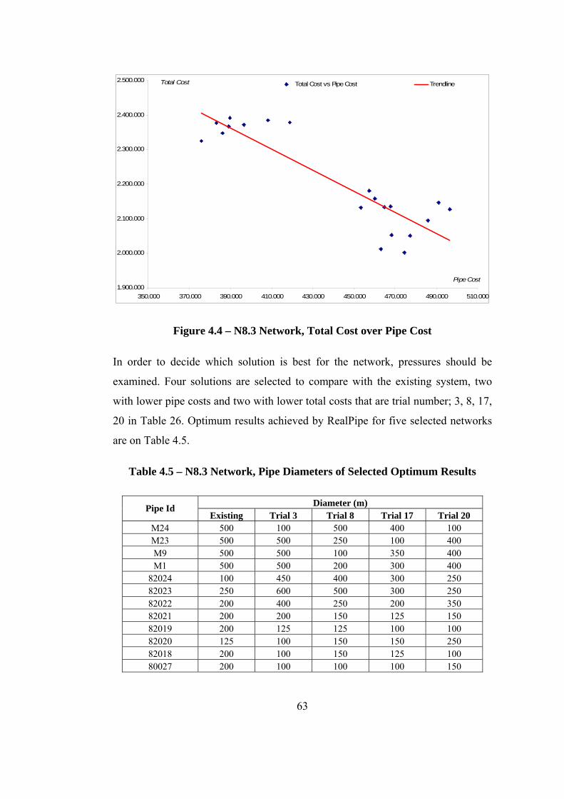
63

1.900.000

2.000.000

2.100.000

2.200.000

2.300.000

2.400.000

2.500.000

350.000 370.000 390.000 410.000 430.000 450.000 470.000 490.000 510.000

Pipe Cost

Total Cost Total Cost vs Pipe Cost Trendline

Figure 4.4 – N8.3 Network, Total Cost over Pipe Cost

In order to decide which solution is best for the network, pressures should be

examined. Four solutions are selected to compare with the existing system, two

with lower pipe costs and two with lower total costs that are trial number; 3, 8, 17,

20 in Table 26. Optimum results achieved by RealPipe for five selected networks

are on Table 4.5.

Table 4.5 – N8.3 Network, Pipe Diameters of Selected Optimum Results

Diameter (m) Pipe Id Existing Trial 3 Trial 8 Trial 17 Trial 20

M24 500 100 500 400 100 M23 500 500 250 100 400 M9 500 500 100 350 400 M1 500 500 200 300 400

82024 100 450 400 300 250 82023 250 600 500 300 250 82022 200 400 250 200 350 82021 200 200 150 125 150 82019 200 125 125 100 100 82020 125 100 150 150 250 82018 200 100 150 125 100 80027 200 100 100 100 150

64

Table 4.5 (continued)

Diameter (m) Pipe Id Existing Trial 3 Trial 8 Trial 17 Trial 20

82008 150 100 100 100 100 82009 150 125 125 100 100 82007 200 125 125 200 100 82006 150 350 125 250 125 82005 100 200 250 100 150 82003 250 200 450 125 125 82012 200 100 125 100 200 82002 250 125 100 100 150 82014 150 125 125 125 125 82015 150 150 450 600 500 82010 150 100 100 100 100 82013 100 125 125 125 200 82001 250 450 400 250 125 83020 150 100 100 150 150 82004 150 250 250 150 200 82011 125 100 125 125 125 83019 125 125 200 100 250 83018 125 125 125 200 250 83016 125 400 300 200 350 83015 125 100 250 200 500 83014 100 600 150 300 450 83013 100 100 125 125 400 83021 250 100 100 250 125 83011 125 125 125 125 150 83007 125 500 250 150 150 83008 100 250 125 150 150 83006 100 250 150 125 450 83012 250 150 150 200 125 83017 125 200 350 450 400 83010 150 100 100 100 125 83009 150 150 100 100 125 82025 100 150 100 100 100 82026 150 125 100 100 100 83002 100 100 125 125 200 83001 100 100 125 125 100 83003 150 250 150 125 125 83005 250 500 150 250 400 83004 250 400 350 500 250 85023 100 100 100 125 600 85022 100 100 100 150 125 85021 200 100 100 100 200 84011 150 600 500 100 300 84012 150 100 100 300 125

65

Table 4.5 (continued)

Diameter (m) Pipe Id Existing Trial 3 Trial 8 Trial 17 Trial 20

84010 200 125 125 150 150 84002 200 125 100 150 200 84003 100 100 125 250 150 84004 150 150 450 125 200 84009 150 100 100 300 125 84001 100 125 100 100 125 84007 100 150 125 150 200 84006 125 100 250 125 450 84005 150 250 300 350 250 84008 150 200 200 150 125 85020 150 125 300 500 300 85019 150 125 150 150 150 85024 150 125 250 125 500 85012 200 100 250 125 250 85011 200 500 200 100 150 85013 125 100 500 400 100 85014 100 125 125 100 150 85015 125 350 200 300 250 85016 200 400 250 100 250 85017 125 150 100 125 200 85018 200 100 350 200 250 85005 200 200 100 100 250 85002 100 125 125 250 150 85001 100 100 125 100 200 85003 100 125 125 150 100 85004 200 150 150 125 400 85008 150 150 100 250 100 85007 150 100 125 150 100

Pipe Cost (YTL) 451,475 463,271 383,316 375,884 453,371 Total Cost (YTL) 2,012,622 2,376,106 2,325,425 2,131,344

Related pressures at the nodes are shown in Table 4.6. Unsatisfied nodes are

highlighted.

66

Table 4.6 – N8.3 Network, Pressure Heads of Selected Optimum Results

Pressure Heads at the nodes (m) Junction ID

Existing Trial 3 Trial 8 Trial 17 Trial 20 3147 30.40 31.78 30.28 30.29 31.39 3212 55.36 56.15 54.20 55.25 55.82 3286 37.58 38.06 36.62 37.29 37.81 416 30.76 32.49 30.99 31.00 32.08 411 33.66 35.40 33.89 33.90 34.95 160 29.88 31.63 30.11 30.09 31.17 113 23.12 24.86 23.29 23.30 24.40 3078 52.39 53.89 52.44 52.39 53.45 122 37.93 39.53 38.02 38.00 39.21 133 55.23 56.73 55.18 55.20 56.27 138 67.55 69.04 67.47 67.50 68.58 3144 39.31 40.96 38.97 39.60 40.48 100 20.72 22.39 20.78 20.91 21.87 419 24.08 25.68 24.08 24.09 25.14 103 30.15 31.91 30.29 30.36 31.38 420 52.10 53.61 52.05 52.07 53.15 109 57.54 59.05 57.49 57.51 58.59 589 71.48 73.15 71.54 71.67 72.65 591 80.04 81.68 80.10 80.30 81.13 3213 80.20 81.83 80.25 80.45 81.29 588 17.92 19.65 17.98 18.17 19.19 587 32.41 34.10 32.08 32.72 33.60 624 36.94 38.63 36.61 37.25 38.13 618 49.70 51.38 49.37 50.01 50.89 612 75.12 76.66 74.64 75.30 76.15 629 61.67 63.29 61.27 61.92 62.79 628 61.88 63.49 61.47 62.12 62.99 631 36.69 38.32 36.30 36.95 37.82 578 30.66 32.45 30.03 30.82 31.91 575 51.42 53.22 50.79 51.58 52.68 595 67.95 69.75 67.33 68.13 69.23 580 26.41 28.20 26.02 26.81 27.72 3221 46.51 48.13 46.01 46.80 47.74 3222 46.66 48.27 46.15 46.95 47.89 607 58.70 59.96 57.85 58.87 59.57 3209 53.95 52.99 54.49 54.66 56.37 3299 53.39 52.41 53.91 54.13 55.79 782 51.27 50.19 51.81 52.01 53.65 511 55.84 56.77 54.83 55.88 56.39 3300 55.72 56.35 55.36 56.26 57.14 822 53.86 54.12 54.34 55.31 56.25 3830 71.22 70.16 72.09 71.93 73.79

67

Table 4.6 (continued)

Pressure Heads at the nodes (m) Junction ID

Existing Trial 3 Trial 8 Trial 17 Trial 20 1910 67.30 66.17 67.97 67.99 69.88 774 33.59 32.14 34.54 33.90 35.91 771 46.62 45.41 47.81 47.18 49.15 3285 47.12 45.91 48.30 47.64 49.65 784 46.63 45.51 47.35 47.32 49.36 783 48.16 47.04 48.73 48.88 50.57 823 55.10 53.95 55.64 55.86 57.55 813 46.37 45.23 46.93 47.15 48.78 817 52.85 51.74 53.40 53.02 55.30 790 68.59 67.38 69.02 68.86 71.05 819 41.53 40.33 41.94 41.77 43.99 799 71.77 70.58 72.20 72.06 74.24 820 42.97 41.77 43.38 43.21 45.43 801 33.91 32.71 34.53 34.52 36.38 794 31.25 30.19 31.87 32.11 33.73 802 34.47 33.41 35.08 35.10 36.95 785 42.69 41.59 43.38 43.38 45.12 780 41.53 40.43 42.22 42.22 43.96

Pipe Cost (YTL) 451,475 463,271 383,316 375,884 453,371

Total Cost (YTL) 2,012,622 2,376,106 2,325,425 2,131,344

Pressure constraint could not be satisfied at some points on the existing networks

that are highlighted. Real pipe results also could not succeed to solve the pressure

problem except one node, 160. It can be easily concluded that, these areas are

problematic areas and could not be solved only by changing pipe diameters. Some

other precautions should be taken such as introducing pumps and/or tanks.

By definition, an optimization problem requires the satisfaction of the objective

function and constraints. However, genetic algorithm, due to its nature, produces

solutions where some of the constrains are not fulfilled. (Savic and Walters (1997),

Cunha and Sousa (1999))

68

If these unsatisfied nodes are compared with the RealPipe results, almost all results

have higher pressures that the nodes of existing one. Solutions with lower total

costs make more improvements than higher total costs. However these differences

are very small. Tendency to select the network from the solution set should be the

smallest total pipe cost.

Since there are too many pipes and the network is complicated, solution space is

much larger than the previous examples. Solution is user dependent at this case.

Author’s solution is trial 17 which is the solution with lowest total pipe cost. The

total cost achieved by RealPipe is 16.74 percent lower than the existing system and

also this solution hydraulically improved.

69

Figure 4.5 – N8.3 Network, Pressures of Selected Network

70

Figure 4.6 – N8.3 Network, Pipe Diameters of Selected Network

71

Figure 4.7 – N8.3 Network, Velocities of Selected Optimum Network

72

CHAPTER 5

5. CONCLUSION

5.1 – Summary of the Study

The capital cost of a water distribution network including its initial cost, cost of

repair, maintenance, and operation is huge; that’s why researchers are searching

for new methods to obtain more economical designs. However, the determination

of the optimal design of a water distribution network is very complex. In addition

to the capital cost and different elements of the operational costs, an integral

design of a water distribution network should consider not only pipe cost, but also,

tank cost, pump cost, valve cost and fitting cost. Nevertheless, for the sake of

simplicity, this study deals only with the optimization of pipes of water

distribution networks using a genetic algorithm program, called RealPipe;

RealPipe works in combination with EpaNet.

5.2 – Conclusion

In the light of the results of Shamir and Hanoi networks, it can be concluded that

RealPipe works fairly well. The program can reach the best result almost every

time with Shamir network in couple of minutes with necessary reports. Also for

Hanoi network, the program finds a solution, its total pipe costs between the best

results. Hydraulically, it was the best solution together with Liong and Atiquazzam

(2004) solution.

Selection of parameters in genetic algorithm is a difficult and important task to

accomplish. Therefore, while using Shamir network, genetic algorithm parameters

are studied very carefully.

Effects of the parameters on the solution are examined. Large numbers of

population size (i.e. chromosomes) lead to quicker results but it increases the

program run time. Optimum population size is between 30-70 depending on the

network size (i.e. pipe number) and number of available pipe size. These two

73

network variables also limit the loop number. For smaller networks, less number

of loops can be enough but for bigger networks need more loops are needed to

converge to the solution.

Elitism is one of the most important operators mentioned in the earlier chapters.

Smaller elitism rates can cause the loss of probable optimal solution. On the other

hand larger rates hinder the progress of the population. Mutation operator effect is

very much like the Elitism effect. It acts as if it were fixing a mistake in the nature.

Mutation should be selected around 1-5 percent depending on the network. Larger

ratios of mutation results in adverse effect. It increases randomness and harms the

evolution progress. Crossover rate accelerates information exchange between

chromosomes. Multipoint crossover and higher rates are advisable. Ratio over

ninety percent crossover showed good results in this study.

Previous parameters are dealing with the genetic algorithm itself. Hydraulic

conformity of the network is checked and approved by the penalty functions.

Pressure penalty is the driving factor in the optimization of water distribution

networks. RealPipe uses four different penalty constants, two for pressure, and two

for velocity. Each constraint has above and below target constants separately.

Velocity is the secondary driving penalty. Therefore, balance between these

constants should be maintained carefully. Studies show that pressure penalty

should be around 100 times bigger than velocity penalty. Velocity penalty could be

ignored in some networks. For the pressure penalty, since below values of target

pressure is the most unwanted case, this constant should be higher than the other

one. In this study, it is taken as 100 times bigger than the other.

Relation between total cost and total pipe cost should also be examined carefully.

It is very hard to call one of the solutions with minimum total cost as best solution

in larger networks. Similar solutions should be examined carefully in regard to

their nodal pressures. Tendency to select the network from the solution set should

be the smallest pipe cost.

74

Case study results show that, a total cost with lower value and hydraulically

improved solution is found using RealPipe with respect to the existing Network

N8.3.

5.3 – Future Studies

The future study for this subject should mainly be dealing with the determination

of genetic algorithm parameters. Concentration on this kind of study should be on

the penalty constants.

Also program could be updated even though it is very user friendly and flexible.

Further studies on the genetic algorithm coding of the program may result in more

powerful genetic algorithm structure which improves the program’s convergence.

RealPipe is designed for single loading scenario. Multi loading adaptation of the

program may result in better networks.

Finally, this study assumes constant diameter between two nodes. Variable

diameter study results in improved solution sets.

75

REFERENCES

Abebe, A.J., Solomatine, D.P. (1998), “Application of global optimization to the design of pipe networks”, 3rd International Conferences on Hydroinformatics, Copenhagen, Denmark, pp.989-996

Akdoğan T. (2005). “Design of Optimal Water Distribution System by Optimization Using Reliability Considerations”, M.S. Thesis, Middle East Technical University, CE. Dept., Ankara

Alperovits, E., and Shamir, U. (1977). “Design of Optimal Water Distribution Systems.” Water Resources Research, 13: 885-900, 1977

Cunha, M. da C., and Sousa, J. (1999). “Water distribution network design optimization: simulated annealing approach.” J. Water Resour. Plng. And Mgmt., ASCE, 125(4), 215-221.

Dandy, G. C., Simpson, A. R. and Murphy, L. J. (1996). “An improved genetic algorithm for pipe network optimization.” Water Resour. Res., 32(2), 449-458.

Epanet 2 toolkit, www.epa.gov

Goldberg, D. E. (1989). “Genetic Algorithms in Search Optimization and Machine Learning.” Addison Wesley, MA, USA.

Holland, J. H. (1975) “Adaptation in natural and artificial systems” The University of Michigan Press

Kahraman M. (2003), “Optimal design and expansion of water distribution systems using genetic algorithm”, M.S. Thesis, Dokuz Eylül University

Keleş G. (2005). “Water Distribution Network Design by Partial Enumeration”, M.S. Thesis, Middle East Technical University, CE. Dept., Ankara

Liang, T. (1971). “Design of Conduit System by Dynamic Programming.” J. Hydr. Div., ASCE, 97(3), 383-393.

Liong, S., Md. Atiquazzaman (2004), “Optimal Design of Water Distribution Network Using Shuffled Complex Evolution” Journal of Institution of Engineers, Singapore Vol. 44, Ussue 1

Merzi, N., Şendil, U., Yağız E., Eker, İ., Poyraz S. (1998a), “Hydraulic Modeling Process of N8 Pressure Zone of Ankara Water Distribution Network”, ASKI/METU Joint Rducation and Training Program, 1st Progress Report, Middle East Technical University, CE. Dept., Ankara

Merzi, N., Şendil, U., Yağız E., Eker, İ., Poyraz S. (1998b), “Hydraulic Modeling Process of N8 Pressure Zone of Ankara Water Distribution Network”, ASKI/METU Joint Rducation and Training Program, 2nd Progress Report, Middle East Technical University, CE. Dept., Ankara

76

Morley M.S., Atkinson R.M., Savic D.A., and Walters, G. A. (2000). “GAnet: Genetic algorithm platform for pipe network optimisation”, Advances in Engineering Software, 32 (001). 467-475

Savic, D. A., and Walters, G. A. (1997). “Genetic algorithms for least-cost design of water distribution networks.” J. Water Resour. Plng. and Mgmt., ASCE, 123(2), 67-77.

Sevük, S., Altinbilek, D. (1977), “Principles of Design and Solution of Water Distribution Network with Computers”, Middle East Technical University Faculty of Engineering Publications, Ankara

Simpson, A. R., Murphy, L. J., and Dandy G. C. (1993). “Pipe Network Optimization using Genetic Algorithms.” Paper presented at ASCE, Water Resources Planning and Management Specialty Conference, ASCE, Seattle, USA.

Simpson, A. R., Dandy G. C., and Murphy, L. J. (1994). “Genetic algorithms compared to other techniques for pipe optimization.” J. Water Resour. Plng. and Mgmt., ASCE, 120(4), 423-443.

Simpson, A.R. (2000). "Optimization of design of water distribution systems using genetic algorithms." Slovenian Society of Hydraulic Research, Seminar Series, Vol.1, Ljubljana, Slovenia, 10pp.