Optimization of Union College’s Microgrid

to Meet All Load with a Least-Cost,

Low-Carbon Energy Mix

Caitlin McMahon

ECE 499: Capstone Project

Professor Dosiek

Spring 2020

1

Report Summary

A microgrid is a localized, small scale electric grid that generates some or all of the power used to meet

its load. Union College currently has a microgrid that meets around 70 percent of the campus’ load and is

connected to the main grid. It is made up of a cogeneration plant that uses natural gas from National Grid,

as well as solar photovoltaic panels and wind turbines, which are renewable energy sources. The goal of

this project is to determine the least cost, low-carbon energy mix that meets 100 percent of the campus’

load. The issue with solar and wind power is that they are variable based on time of day, time of year, and

the weather. This is addressed in the planning of Union’s microgrid energy mix through considering

storage and other low-carbon renewable generation. Different options for sizes of photovoltaic panels,

wind turbines and batteries will be inputs to the optimization. After considering various possibilities,

MATLAB is used for linear programming optimization with constraints. The output is input to the

Simulink model designed to replicate Union’s microgrid. This step verifies that the energy mix is reliable

under worst case conditions on the peak load day, and mimics the design process an engineering firm

would undertake for a similar project. The optimal energy mix determined by the code is a hybrid mix

made up of solar photovoltaic (PV) arrays, wind turbines, geothermal power, lithium ion battery storage,

and the current cogeneration plant. Specifically, adding 750kW of PV to the current 63kW on campus,

adding 25kW of wind power to the current 36kW, adding 275kW geothermal generation plant, 4.5 MWh

battery storage, and slightly raising the cogen to an average output of 2MW.

2

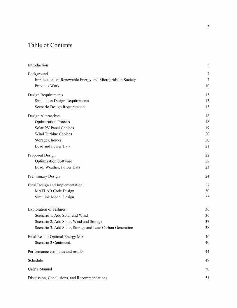
Table of Contents

Introduction 5

Background 7 Implications of Renewable Energy and Microgrids on Society 7 Previous Work 10

Design Requirements 13 Simulation Design Requirements 13 Scenario Design Requirements 13

Design Alternatives 18 Optimization Process 18 Solar PV Panel Choices 19 Wind Turbine Choices 20 Storage Choices 20 Load and Power Data 21

Proposed Design 22 Optimization Software 22 Load, Weather, Power Data 23

Preliminary Design 24

Final Design and Implementation 27 MATLAB Code Design 30 Simulink Model Design 33

Exploration of Failures 36

Scenario 1. Add Solar and Wind 36 Scenario 2. Add Solar, Wind and Storage 37 Scenario 3. Add Solar, Storage and Low-Carbon Generation 38

Final Result: Optimal Energy Mix 40 Scenario 3 Continued. 40

Performance estimates and results 44

Schedule 49

User’s Manual 50

Discussion, Conclusions, and Recommendations 51

3

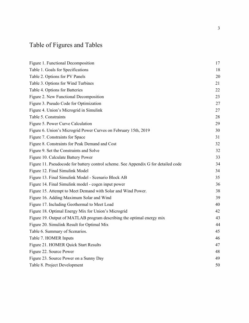
Table of Figures and Tables

Figure 1. Functional Decomposition 17 Table 1. Goals for Specifications 18 Table 2. Options for PV Panels 20 Table 3. Options for Wind Turbines 21 Table 4. Options for Batteries 22 Figure 2. New Functional Decomposition 23 Figure 3. Pseudo Code for Optimization 27 Figure 4. Union’s Microgrid in Simulink 27 Table 5. Constraints 28 Figure 5. Power Curve Calculation 29 Figure 6. Union’s Microgrid Power Curves on February 15th, 2019 30 Figure 7. Constraints for Space 31 Figure 8. Constraints for Peak Demand and Cost 32 Figure 9. Set the Constraints and Solve 32 Figure 10. Calculate Battery Power 33 Figure 11. Pseudocode for battery control scheme. See Appendix G for detailed code 34 Figure 12. Final Simulink Model 34 Figure 13. Final Simulink Model - Scenario Block AB 35 Figure 14. Final Simulink model - cogen input power 36 Figure 15. Attempt to Meet Demand with Solar and Wind Power. 38 Figure 16. Adding Maximum Solar and Wind 39 Figure 17. Including Geothermal to Meet Load 40 Figure 18. Optimal Energy Mix for Union’s Microgrid 42 Figure 19. Output of MATLAB program describing the optimal energy mix 43 Figure 20. Simulink Result for Optimal Mix 44 Table 6. Summary of Scenarios. 45 Table 7. HOMER Inputs 46 Figure 21. HOMER Quick Start Results 47 Figure 22. Source Power 48 Figure 23. Source Power on a Sunny Day 49 Table 8. Project Development 50

4

Introduction

The electric grid is traditionally a large scale, bulk energy system. Power plants generate power which is

sent over transmission lines at high voltages to distribution substations and then to customers at low

voltages. Fossil fuels are used to generate the majority of our electricity, however they are depleting in

supply and have high carbon emissions. This is leading to a rise in the importance of low-carbon,

renewable generation, such as wind and solar power. There are many challenges associated with the

integration of renewables, specifically the variability in power output due to time of day, time of year, and

the weather. This is called intermittency. For example, solar photovoltaic (PV) panels cannot produce

power overnight or when there is cloud cover. Similarly, wind turbines cannot produce power when there

is a lack of wind speed. This is often addressed by adding storage. However, these systems can be more

expensive than conventional systems [1]. Hence, adding renewable, low-carbon sources to an electric grid

requires advanced planning based on weather, load patterns and cost analysis.

Along with the increase in renewable generation, microgrids are becoming a trend in the energy sector. A

microgrid is a localized energy grid [2]. Microgrids can use power from the grid, from their local

generation, or from a combination of both. Generation may come from renewable sources, whether it be

for environmental reasons, or because of the location’s resource of solar or wind. Microgrids can also use

more traditional methods of generation such as diesel or natural gas. A system composed of both

conventional and renewable resources is called a hybrid system [3]. Control mechanisms for microgrids

are often based on minimizing cost while still maintaining reliability. For example, if the microgrid is not

generating enough power, it should draw power from the main grid. If there is enough power to meet

load, it should store the surplus, sell it back to the grid, or curtail it. When there is a problem on the main

5

grid, a microgrid can disconnect and operate on its own, providing increased reliability [4]. This control

capability is useful for many communities, especially hospitals, jails, and college campuses.

Union College’s microgrid currently meets about 70 percent of the load. The goal is to meet 100 percent

of its load so that the microgrid can operate entirely on its own, but remain connected to the grid for

reliability purposes. The hybrid system is made up of a cogeneration plant which provides most of the

power, as well as solar photovoltaic (PV) panels and wind turbines. This paper seeks to find the least cost

combination of low-carbon energy resources to add to the current microgrid to meet all of the campus’

load.

This report will first introduce background information including how renewable energy and microgrids

affect different aspects of society. Then previous work for the optimization of microgrid design will be

discussed. The design requirements for Union’s microgrid and the optimization software will be

described, then alternatives will be explored. This will lead into the discussion of the selected

methodology for this project. The overall objective of this project is to determine the optimal amount of

solar, wind, and possibly storage and other generation to add to the microgrid to meet the campus’ load

under worst case conditions on a peak demand day. The resulting energy mix that meets these

requirements will be explained. Lastly, conclusions and future work will be discussed.

6

Background

Implications of Renewable Energy and Microgrids on Society

For most of our recent history, the electric grid has remained the same large scale system. As the grid is

altered with distributed generation (DG), renewable energy, and microgrids, the energy market becomes

more complex and affects energy prices. This reflects on our society as a whole. Microgrids offer many

benefits such as increased grid reliability and efficiency, and decreased carbon emissions [5]. This is a

great advantage compared to fossil fuels, which have been shown to have a negative impact on the

environment. Hence, government goals such as NYS Governor Cuomo’s Green New Deal have been

announced to help the environment. The deal raises the 2030 renewable energy generation goal from 50 to

70 percent of the electric grid through additional wind and solar resources [6]. As more customers are

buying into DG and microgrids, control schemes are being created, incentives and policies are being

implemented, and regulatory agencies and utilities are being educated, making implementation easier as

time goes on [5].

Microgrids also offer safety benefits, especially for sites that rely on surety of power. For example,

hospitals benefit greatly from having a well-designed, reliable microgrid. When there are issues on the

main grid, the microgrid can disconnect and enter islanding mode. This allows the hospital to keep its

power on and therefore keep its patients alive. This same idea is useful for jails, where a power outage

could result in unlocking of jail cells and create safety risks for the security workers and inmates.

Facilities like these are often prioritized by utilities during outages, but a reliable microgrid ensures

constant supply of power.

7

The downside to renewable energy, as previously mentioned, is intermittency. As we move towards

higher penetration of renewable energy, a lack of proper planning and load analysis could result in the

grid’s inability to meet demand under some circumstances without proper backup [7]. This illustrates the

importance of in depth analysis of renewable energy and the weather at the location of installation. In this

case, designing the additions to Union’s microgrid clearly requires consideration of load and weather

patterns. Making sure the combination of wind and solar energy can supply sufficient power, even on the

worst case days, will be a design requirement for the project.

Another important aspect of this analysis is the differences in a hybrid system with and without storage.

Adding storage to a highly renewable energy based microgrid may have interesting effects on system

reliability and cost. One study noted that placing storage close to generation can increase the voltage

consistency on the grid [8]. This is a benefit of having storage in a microgrid, since all devices are closely

located by definition. Furthermore, this “co-location” results in lower costs because of less hardware

components and labor, as well as government initiatives for “solar plus storage” [9]. Policies encourage

this because storage smooths the variability in the solar generation. Simulating adding storage to Union’s

microgrid will therefore be a part of this project, with the same requirement of minimizing cost while

meeting all load.

Storage has a downside as well. A possible negative effect of batteries is that they may not actually

improve carbon emissions on a large scale without an official carbon tax [10]. This is because batteries

charge when energy is cheap, which is often overnight. During this time, some fossil fuel plants are still

operating at a percentage of their maximum output to avoid ramping restrictions. Hence, there is the

possibility that batteries store some amount of energy generated from fossil fuels, which does not improve

8

the carbon emissions of the energy system [10]. However, this microgrid could be designed so that the

storage unit only charges when there is excess generation of renewable energy. This would improve

carbon emissions in Union’s case. Rather than relying on natural gas from the cogeneration plant when

solar and wind cannot supply enough power to meet demand, storage could supply the excess power that

came from renewable sources. Another aspect of storage that is worth considering is their life cycle and

resulting effect on the environment. When the typical double-A battery “runs out” or dies, we throw it

out. The same will have to happen with large scale batteries. All batteries have different life cycles, and as

the technologies develop, life cycles are often increasing. However, adding storage to a microgrid at this

point may still have a negative environmental impact since it cannot be recycled, and chemical waste does

not align with the greener, sustainable aspects of a microgrid. However for Union’s case, a battery may

help reach the goal of supplying all demanded power in a carbon friendly way since it would be storing

mostly renewable energy.

Microgrid design tools like the ones discussed in the section below, and the one I am seeking to develop,

can help advance the implementation of renewable energy in microgrids. Another advantage of

developing systems like these is that policy makers and government officials who were not previously

aware of the science behind the electric grid can see how systems work optimally. Those who create

incentives for renewable energy can also explore the most cost effective systems [11]. This will all result

in better planning and hence benefits for electricity customers. Another research paper discusses the

impact that renewable energy and microgrids have on politics and policies. It claims that changes to the

power sector are crucial to combat climate change, and power electronics “will be a key element in the

energy policies of nations” [12].

9

Lastly, ethics are always necessary to discuss for any project. As for this paper, there are few ethical

implications. There are no obvious ways in which the findings of this paper could be used in a bad way,

and no harm can come from the actual installation of more wind turbines and solar panels on campus as

long as it is done by professionals who know the proper techniques. The only apparent ethical issue with

renewable energy is potential increased costs without incentives to lower energy costs on utility scale. On

a large scale, if more energy comes from renewable energy, or if there is ever a carbon tax implemented,

the cost of energy could potentially increase. This could negatively affect people with low incomes.

However this is only applicable on utility scale, since on a small scale, the customer(s) would be

purchasing the system themselves, knowing the associated costs. Furthermore, a microgrid usually results

in decreased costs. Since minimizing cost is the basis of this project, this ethical concern is being

considered.

Previous Work

There are various research papers discussing approaches to optimizing the design of microgrids. One

study developed a model called Regional Renewable Electricity Economic Optimization Model

(RREEOM) which simulates a renewable power based grid with the goal of obtaining the combination of

generation and storage to minimize cost while reliably supplying the load [13]. This study provides

valuable information to my project, however it is focused on a large regional electric grid rather than a

microgrid. It was found that generating two to three times the electricity needed to meet electrical load

was the least cost option, depending on the circumstances and initial conditions of weather and load. I will

consider this by not initially constraining the system to a maximum number of PV or turbines. However,

depending on the results, I may have to limit this due to space for the additions. The same study also

showed that higher storage actually increased system costs with the technologies available. My project

10

will analyze both cases, with and without storage. Another conclusion from the study is that combining

different types of renewable energy provided more stability on the grid [13]. Although since this study

was based on a large scale with widely diverse generation sources at diverse locations, these findings have

a limited, but still insightful, implication to a microgrid study.

HOMER is a tool developed by NREL that optimizes microgrid design and sizing. HOMER takes

multiple inputs including the cost and capacity of generation sources, the location of the grid, and the load

profile. Then it tests different combinations of resources and produces various options and prices [11].

Various studies utilize this tool [14-17]. One research paper tested a system with only PV, with only wind

turbines, then with PV, turbines and batteries. HOMER determined the least cost, most reliable energy

mix was the combined hybrid system [15]. A similar study on the design of a microgrid for a water

treatment plant recommended a solar-wind hybrid over a solely wind based system [17]. Clearly, a more

diverse combination of resources is often better than just one type of energy source. The water treatment

plant study utilized HOMER software because it was determined to be the best for their microgrid

application. Other programs considered were EnergyPlan, which is a deterministic model and not suitable

for this problem, and H2RES, which was not selected due to inability to simulate grid connection. Since

Union needs to remain grid connected, H2RES cannot be utilized for my simulation either. HOMER is

not a free tool, but will be used as a comparison to what my model and optimization process produces.

A model of a microgrid based on wind, PV, and battery combinations was created by Ramos and Ramos

[18]. Their research demonstrates how solar and wind can complement each other, since wind is often

stronger at night and during the winter months, whereas solar can provide more energy during the day and

the summer months. A higher ratio of wind to solar was optimal, while higher reliance on PV resulted in

higher system costs. This is due to geographical factors and the weather. However, in Schenectady, the

11

location and weather factors are different and need to be studied. Therefore, my design will include

location specific wind and solar irradiance data.

An optimization of a residential energy supply (RES) system used linear programming and modeled the

grid using only equations [1]. This is a limited approach because it only offers optimization of PV, a solar

thermal collector, and a heat pump. Furthermore, the entire modeling and optimization process has

application limitations due to broad assumptions.

REMix is another software developed to determine a “Renewable Energy Mix for Sustainable Electricity

Supply” [19]. This tool considers a much larger scale than a microgrid - it investigates energy mixes for

various countries in Europe and North Africa. One interesting topic this paper makes note of is the effect

of politics on the energy sector, which in turn affects all users of electricity. Since renewable energy and

storage technologies are newer and more expensive, if policy makers do not incentivize programs to

encourage implementation of these environmentally friendly sources, they may not be implemented. The

REMix model takes into account the availability and cost of renewable energy, transmission, and storage

to determine the size and locations of equipment which makes up a power system that minimizes cost.

Since my project will not have any transmission lines and is a much smaller scale than an entire country,

some aspects of the design of this software are not relevant. However, this model also uses linear

programming as the method of optimization, which illustrates that linear programming is sufficient for my

needs.

12

Design Requirements

The purpose of this project is to determine the optimal low-carbon energy mix for Union’s microgrid in

order to meet 100 percent of the load at a minimum cost. Since this project simulates the options that

could possibly be implemented, there are two subsections of design requirements: one for the simulation

itself, and one for the scenarios which may be actually implemented.

Simulation Design Requirements

The simulation must have a practical run time of less than twenty minutes. The optimization must

consider the peak load day. For solar and wind, the optimization must also consider the days with the low

irradiance and wind speed, respectively, to make sure enough power can be generated to meet all load

even under these worst case conditions. The optimization must minimize the cost function, which is the

total cost of additions, while meeting all load.

Scenario Design Requirements

Based on the literature review above, a scenario with PVs and wind turbines should be analyzed, as well

as a combined system with PVs, turbines, and storage. If this is not attainable, extra generation should be

added. This creates the three scenarios which will be explored in this paper. Each scenario needs to be

able to meet all of Union’s load on the peak day, or else it cannot be considered optimal. Currently the

microgrid can supply up to 70 percent of the campus’ load, which peaks at approximately 2.9MW

according to National Grid data. The cogeneration plant supplies most of the load, averaging around

13

1.8MW, with solar panels providing about 63kW and the wind turbine providing less than 36kW. Hence,

to reach 100 percent of the campus’ load, there needs to be approximately 1MW of added power

generation to meet the peak of 2.9MW. Based on [13], the microgrid may require more than this to

reliably meet load, due to the variability in power supply from PVs and turbines. The simulation will

reveal how much extra power needs to be added.

Another design requirement is the cost limitation. When Union added the cogeneration plant, a grant of

$12 million total was awarded for the project [20]. For the purposes of this paper, it will be assumed that a

similar grant amount could be awarded. Hence, the cost of additions for each scenario must be less than

$12 million in order for the college to consider implementing it.

Equipment and grid design are other important considerations for this project. The scenario needs to have

the option to remain grid tied for emergencies. The equipment needed for each scenario must be easily

available on the market, and meet all of the relevant standards for the respective piece of equipment.

Along with these requirements, the scenarios must meet additional specific requirements:

1. Add PV panels and wind turbines to meet load

This scenario requires space availability for wind turbines and PV panels. The results of the optimization

must be analyzed closely to determine if the amount of PV panels and turbines could realistically be

installed on campus. Because of solar and wind intermittency, there must be a control scheme

implemented to determine when to use the cogeneration plant’s power. The cogenerator should remain at

least slightly on at all times to avoid ramping up and ramping down which is expensive, in terms of

money and energy. The control scheme should use the minimum amount of power from the cogenerator

14

as possible to avoid this while using the maximum amount of wind and solar power to meet load. When

there is not enough wind power due to lack of wind, and not enough solar due to lack of sun, the

cogenerator should increase its output to match the load. This is similar to two research papers which both

developed a control scheme to limit PV power output only when the diesel generator is at its lowest and

demand is still being met [8, 13].

2. Add PV panels, wind turbines and storage to meet load

This scenario builds on the previous one by adding storage. This can help the college use more power

generated on site, rather than buying gas from National Grid. Hence, this scenario has potential economic

advantages, but the cost of the storage may limit the benefits [13]. The control scheme for this case will

build upon the previously described one. When the minimum power output of the cogenerator plus the

maximum output of the solar panels and/or wind turbines supply more power than demanded, the excess

power can be stored. This avoids curtailment, which is defined as limiting the output of renewable energy

sources when there is less power demanded than how much power the source could produce [2]. When

there is not enough solar and wind output plus the minimum cogenerator output to meet demand, the

stored power should be used. If there is not enough stored power to compensate, the cogenerator should

increase its output. This control scheme aims to maximize environmentally friendliness by using

renewable sources of energy plus storage as much as possible, while also minimizing cost by producing as

much as possible onsite before buying more gas from the grid.

15

3. Add PV panels, wind turbines, storage and extra low-carbon generation to meet load

If scenarios 1 and 2 do not produce a reliable, low cost energy mix, extra generation may have to be

added. Marc Donovan, Head of Facilities at Union College, said that the college is considering adding

geothermal generation, which is considered a renewable resource and produces 99% less carbon dioxide

than fossil fuel plants [21]. This is typically used as a baseload power source, similar to the cogen, and

stays on for a certain output around the clock. This could help provide enough generation to complement

solar, wind and storage to meet load all day. Geothermal costs about $2500/kW on average [22].

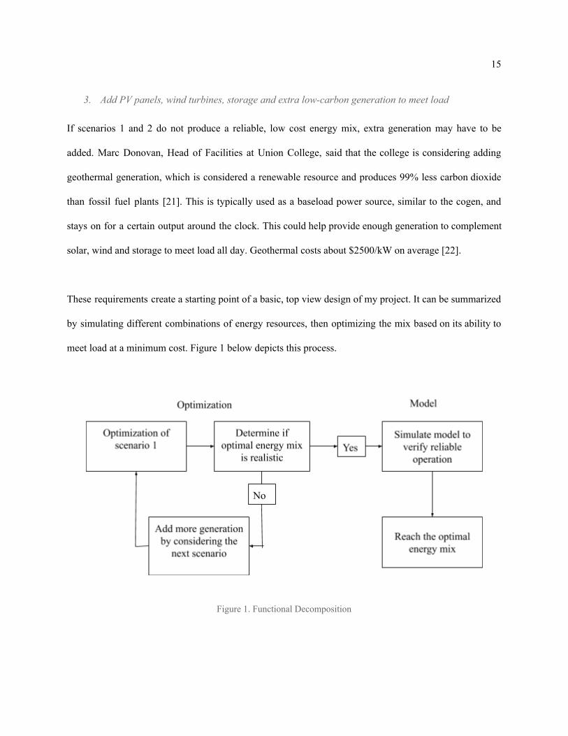
These requirements create a starting point of a basic, top view design of my project. It can be summarized

by simulating different combinations of energy resources, then optimizing the mix based on its ability to

meet load at a minimum cost. Figure 1 below depicts this process.

Figure 1. Functional Decomposition

16

The first loop in Figure 1 will optimize the amount of generation from the sources proposed in each

scenario based on cost and power output. It will start with scenario 1, check if it is realistic, then go to the

next scenario if not. This will continue until the energy mix output is realistically constrained, then the

result should be modeled for verification and further understanding.

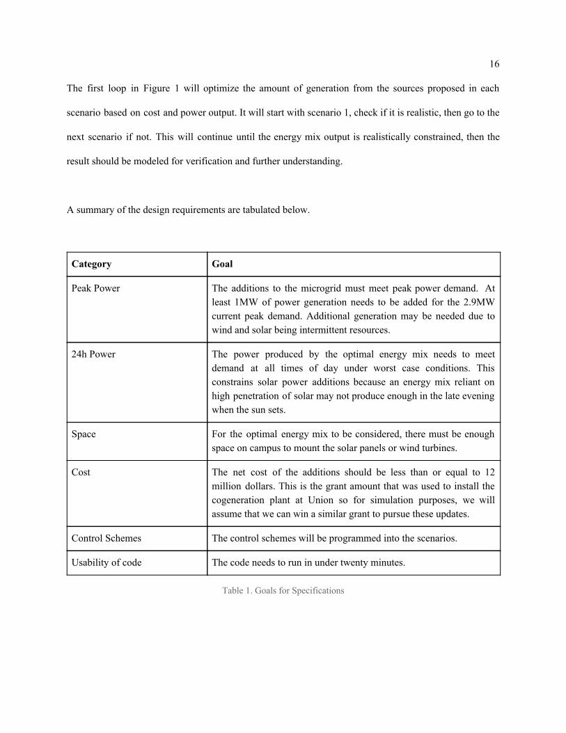
A summary of the design requirements are tabulated below.

Category Goal

Peak Power The additions to the microgrid must meet peak power demand. At least 1MW of power generation needs to be added for the 2.9MW current peak demand. Additional generation may be needed due to wind and solar being intermittent resources.

24h Power The power produced by the optimal energy mix needs to meet demand at all times of day under worst case conditions. This constrains solar power additions because an energy mix reliant on high penetration of solar may not produce enough in the late evening when the sun sets.

Space For the optimal energy mix to be considered, there must be enough space on campus to mount the solar panels or wind turbines.

Cost The net cost of the additions should be less than or equal to 12 million dollars. This is the grant amount that was used to install the cogeneration plant at Union so for simulation purposes, we will assume that we can win a similar grant to pursue these updates.

Control Schemes The control schemes will be programmed into the scenarios.

Usability of code The code needs to run in under twenty minutes.

Table 1. Goals for Specifications

17

Design Alternatives

Optimization Process

To optimize an objective function, many software programs could be utilized. In a review of current

technologies available, there were over 75 programs listed and explored [7]. One of the programs

mentioned was CYME, which I have access to through my internship at National Grid. However I do not

have the ability to program an optimization such that energy resources are changed or added, I am only

able to study what is currently there. On the system, Union is simply modeled as a load, so I would have

to design the microgrid myself, making CYME no better than other alternatives.

I also considered Python Anaconda, PSCAD, MATLAB, and HOMER. A similar research project created

a model of a renewable energy based grid consisting of a wind turbine and a solar panel on PSCAD [8].

To create the turbine, factors such as measured wind speed data, turbine and other mechanical efficiency

factors, and electrical efficiencies were considered. To create the solar panel, an inverter modeled as a

current source was used. For my own project, I would have to learn PSCAD or Python, while I already

have experience with MATLAB. The wind turbine and solar panels are modeled in a similar way in the

Small Scale Microgrid model on MATLAB Simulink [23]. Furthermore, MATLAB has a toolbox of

optimization abilities.

18

Optimization Method

Regardless of the software, there are various methods of optimization. Following similar grid design

studies such as [1], a linear optimization approach is suitable. Again, linear optimization or “linear

programming” is simply optimization of a linear function. A subcategory of this is mixed integer linear

optimization. This means some of the constraints are integers [24]. In this case, the number of solar panels

and wind turbines are integer values. Quadratic optimization is another method, however it is for

nonlinear applications and is therefore not necessary [25].

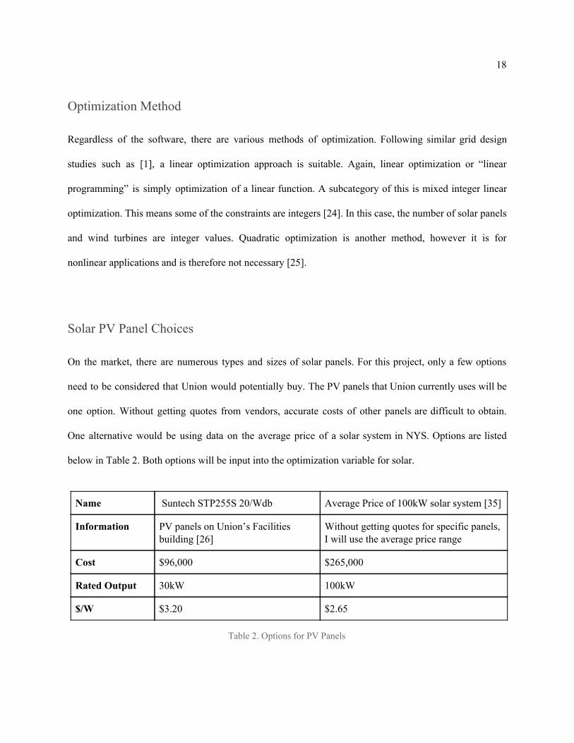
Solar PV Panel Choices

On the market, there are numerous types and sizes of solar panels. For this project, only a few options

need to be considered that Union would potentially buy. The PV panels that Union currently uses will be

one option. Without getting quotes from vendors, accurate costs of other panels are difficult to obtain.

One alternative would be using data on the average price of a solar system in NYS. Options are listed

below in Table 2. Both options will be input into the optimization variable for solar.

Name Suntech STP255S 20/Wdb Average Price of 100kW solar system [35]

Information PV panels on Union’s Facilities building [26]

Without getting quotes for specific panels, I will use the average price range

Cost $96,000 $265,000

Rated Output 30kW 100kW

$/W $3.20 $2.65

Table 2. Options for PV Panels

19

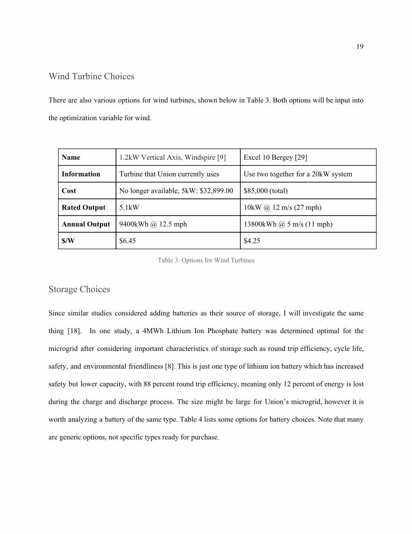
Wind Turbine Choices

There are also various options for wind turbines, shown below in Table 3. Both options will be input into

the optimization variable for wind.

Name 1.2kW Vertical Axis, Windspire [9] Excel 10 Bergey [29]

Information Turbine that Union currently uses Use two together for a 20kW system

Cost No longer available, 5kW: $32,899.00 $85,000 (total)

Rated Output 5.1kW 10kW @ 12 m/s (27 mph)

Annual Output 9400kWh @ 12.5 mph 13800kWh @ 5 m/s (11 mph)

$/W $6.45 $4.25

Table 3. Options for Wind Turbines

Storage Choices

Since similar studies considered adding batteries as their source of storage, I will investigate the same

thing [18]. In one study, a 4MWh Lithium Ion Phosphate battery was determined optimal for the

microgrid after considering important characteristics of storage such as round trip efficiency, cycle life,

safety, and environmental friendliness [8]. This is just one type of lithium ion battery which has increased

safety but lower capacity, with 88 percent round trip efficiency, meaning only 12 percent of energy is lost

during the charge and discharge process. The size might be large for Union’s microgrid, however it is

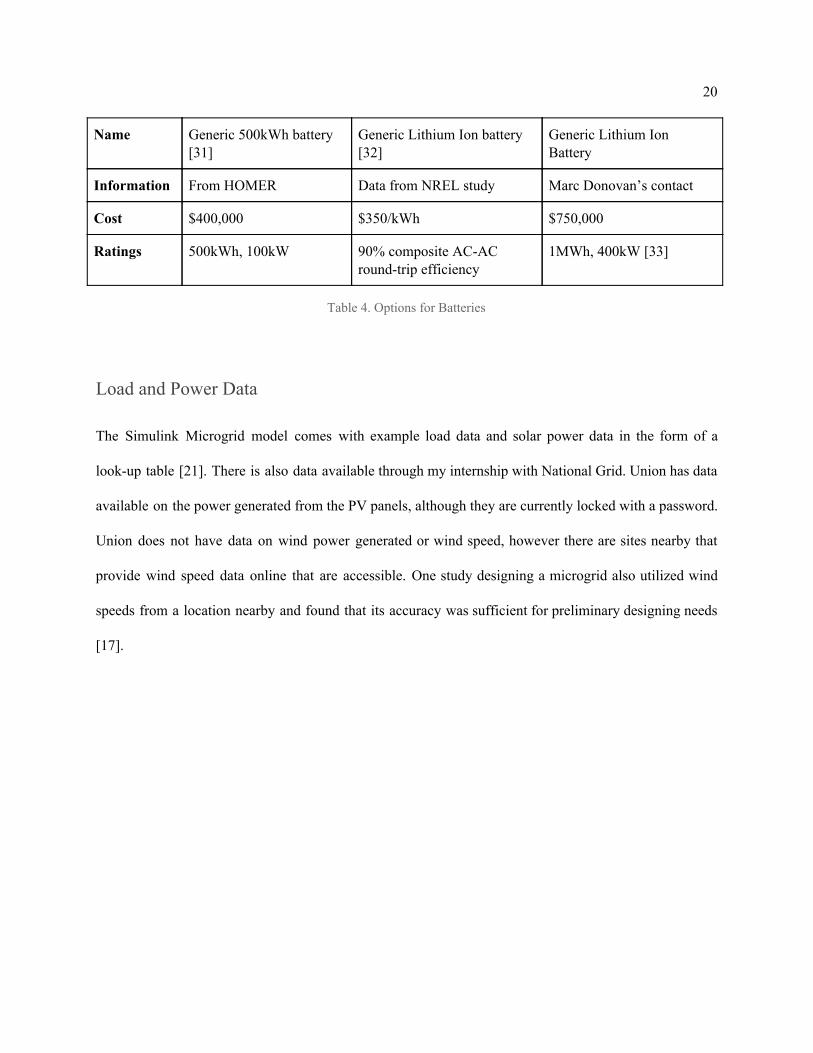
worth analyzing a battery of the same type. Table 4 lists some options for battery choices. Note that many

are generic options, not specific types ready for purchase.

20

Name Generic 500kWh battery [31]

Generic Lithium Ion battery [32]

Generic Lithium Ion Battery

Information From HOMER Data from NREL study Marc Donovan’s contact

Cost $400,000 $350/kWh $750,000

Ratings 500kWh, 100kW 90% composite AC-AC round-trip efficiency

1MWh, 400kW [33]

Table 4. Options for Batteries

Load and Power Data

The Simulink Microgrid model comes with example load data and solar power data in the form of a

look-up table [21]. There is also data available through my internship with National Grid. Union has data

available on the power generated from the PV panels, although they are currently locked with a password.

Union does not have data on wind power generated or wind speed, however there are sites nearby that

provide wind speed data online that are accessible. One study designing a microgrid also utilized wind

speeds from a location nearby and found that its accuracy was sufficient for preliminary designing needs

[17].

21

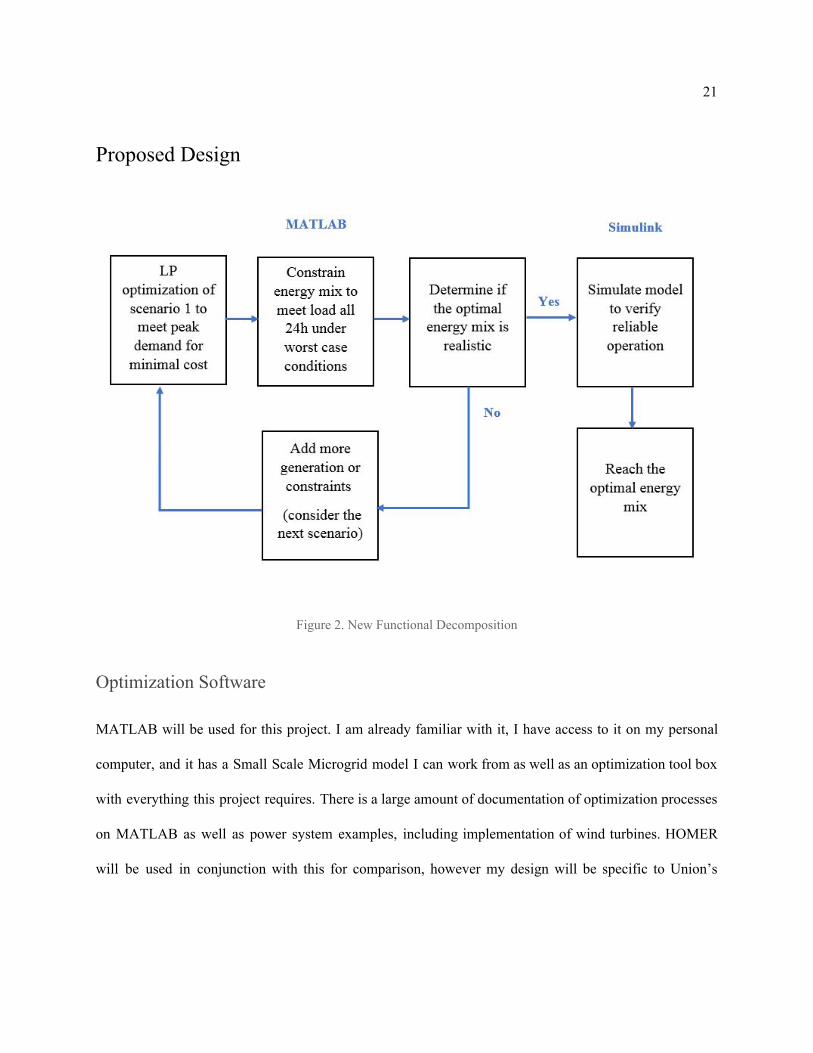
Proposed Design

Figure 2. New Functional Decomposition

Optimization Software

MATLAB will be used for this project. I am already familiar with it, I have access to it on my personal

computer, and it has a Small Scale Microgrid model I can work from as well as an optimization tool box

with everything this project requires. There is a large amount of documentation of optimization processes

on MATLAB as well as power system examples, including implementation of wind turbines. HOMER

will be used in conjunction with this for comparison, however my design will be specific to Union’s

22

needs and have the benefit of simulating our microgrid. Linear programming will be used for the

minimization of the objective function.

Objective Function

In a microgrid design study, the objective function was the overall cost of the energy system [1]. I will

follow the same idea, using MATLAB documentation as a reference for set-up [34]. Figure 3 at the end of

this section illustrates how this will be carried out. First I will explain other choices for my system.

Equipment

The objective function will be programmed to compare the options for the PV panels, wind turbines, and

batteries. Then it will choose the type, size, and number of each that minimizes the cost functions along

with the other variables. Hence, all of the information in Tables 2, 3, and 4 will be input into MATLAB.

Load, Weather, Power Data

The other crucial inputs into the optimization are data on load, weather, and power production. To choose

the peak load day, I utilized an excel tool through National Grid called PI Datalink. I downloaded data for

the maximum power that Union bought from the grid each month in 2019, then filtered to find the day

which had the highest overall value in that month. I determined that February 15th was the day with the

highest amount of power bought from National Grid in 2019. Since what we use on campus is a mix of

power from National Grid with power produced by the cogen, I obtained the power metered for the cogen

23

plant. I added them together to obtain a preliminary peak day load curve for Union. It still needs to

consider the wind and solar power used on this day.

For solar power, I am using the data that is automatically in the Simulink Small Scale Microgrid model. I

scaled it so that the peak is 63kW, which is the current amount of installed solar PV on campus. I add this

resulting generation curve to the demand, assuming that solar was able to produce that much on February

15th. Overestimating the amount of solar power produced on this day will only make this study more

reliable, by assuming demand on the grid is slightly higher than it actually may have been after

considering solar power. One study shows that the placement and angle of the PV panel plays a role in

power production [17]. Since my study does not include determining specific locations of the PV panels

and wind turbines, average data can be used to simulate. To create a worst case day, I decrease the

amount of power produced by solar by 20%.

For the wind data, I gathered 24 hours of wind speed (m/s) from a site in Albany. This is the closest

obtainable wind speed information to campus. Since wind power is proportional to wind speed, I scaled

the wind speed data to match peak wind power production. This is not entirely accurate because the wind

speed in Albany is not necessarily representative of that at different locations on campus. To create the

least windy day for the worst case conditions, I simply scaled down the wind power produced by 20%.

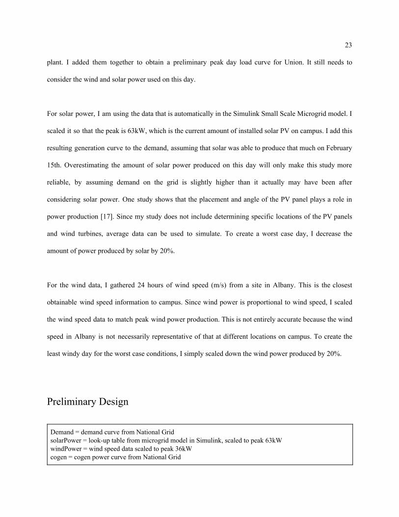
Preliminary Design

Demand = demand curve from National Grid solarPower = look-up table from microgrid model in Simulink, scaled to peak 63kW windPower = wind speed data scaled to peak 36kW cogen = cogen power curve from National Grid

24

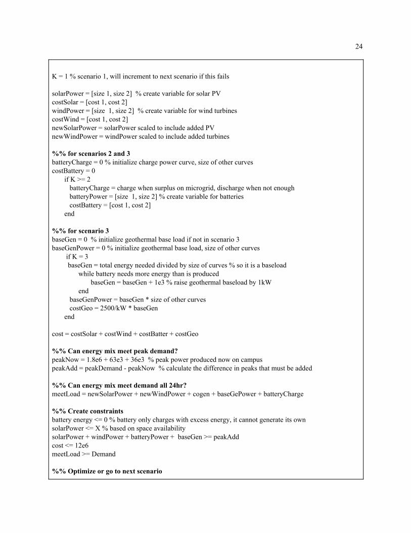
K = 1 % scenario 1, will increment to next scenario if this fails solarPower = [size 1, size 2] % create variable for solar PV costSolar = [cost 1, cost 2] windPower = [size 1, size 2] % create variable for wind turbines costWind = [cost 1, cost 2] newSolarPower = solarPower scaled to include added PV newWindPower = windPower scaled to include added turbines %% for scenarios 2 and 3 batteryCharge = 0 % initialize charge power curve, size of other curves costBattery = 0 if K >= 2 batteryCharge = charge when surplus on microgrid, discharge when not enough batteryPower = [size 1, size 2] % create variable for batteries costBattery = [cost 1, cost 2] end %% for scenario 3 baseGen = 0 % initialize geothermal base load if not in scenario 3 baseGenPower = 0 % initialize geothermal base load, size of other curves if K = 3 baseGen = total energy needed divided by size of curves % so it is a baseload while battery needs more energy than is produced baseGen = baseGen + 1e3 % raise geothermal baseload by 1kW end baseGenPower = baseGen * size of other curves costGeo = 2500/kW * baseGen end cost = costSolar + costWind + costBatter + costGeo %% Can energy mix meet peak demand? peakNow = 1.8e6 + 63e3 + 36e3 % peak power produced now on campus peakAdd = peakDemand - peakNow % calculate the difference in peaks that must be added %% Can energy mix meet demand all 24hr? meetLoad = newSolarPower + newWindPower + cogen + baseGePower + batteryCharge %% Create constraints battery energy <= 0 % battery only charges with excess energy, it cannot generate its own solarPower <= X % based on space availability solarPower + windPower + batteryPower + baseGen >= peakAdd cost <= 12e6 meetLoad >= Demand %% Optimize or go to next scenario

25

optimize(cost) Plot resulting energy mix if optimization fails, K = K + 1 else Update Simulink model and verify it still meets load end

Figure 3. Pseudo Code for Optimization

Based off of the Small Scale Microgrid Model in Simulink, I have modelled what Union’s microgrid is

currently designed as in Figure 4.

Figure 4. Union’s Microgrid in Simulink

26

On the far left, the three phase source represents National Grid. Then we have the wind turbine, three

phase RLC load, then it breaks out into single phase to represent the on-campus distribution network.

Transformers step the voltage down from 13.2kV to 120/240V. The solar panels are on the single phase

portion because they are tied in to the circuit of the building which they are mounted on. The house

blocks represent the loads on each phase. The solar panels and houses are current sources. Each phase is

balanced. The currents are calculated from the solar and load power in MATLAB and divided by three, so

each phase has ⅓ of the total power. More detail is discussed in the final design section.

Final Design and Implementation

Final Constraints to Energy Mix

This term I met with Marc Donovan, Head of Facilities at Union College, to get accurate numbers that

represent and constrain Union’s microgrid. I also gathered information from National Grid.

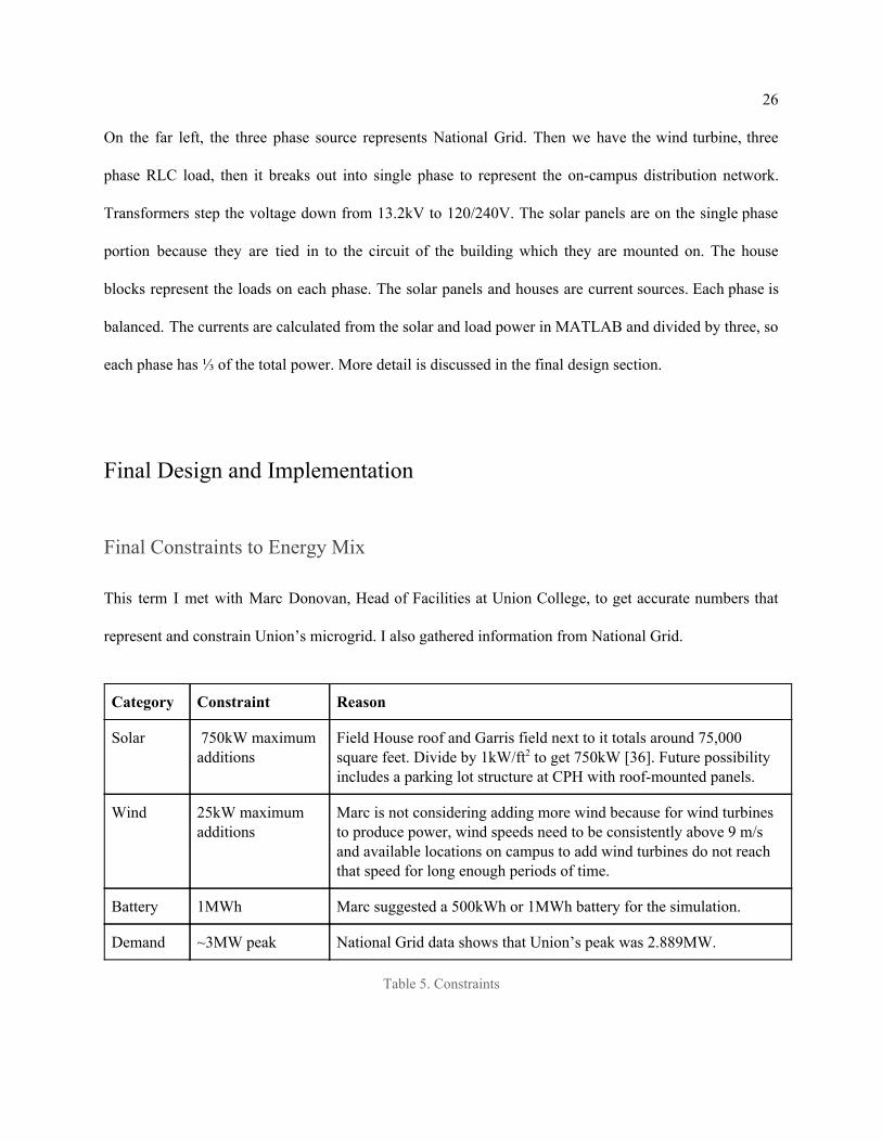
Category Constraint Reason

Solar 750kW maximum additions

Field House roof and Garris field next to it totals around 75,000 square feet. Divide by 1kW/ft2 to get 750kW [36]. Future possibility includes a parking lot structure at CPH with roof-mounted panels.

Wind 25kW maximum additions

Marc is not considering adding more wind because for wind turbines to produce power, wind speeds need to be consistently above 9 m/s and available locations on campus to add wind turbines do not reach that speed for long enough periods of time.

Battery 1MWh Marc suggested a 500kWh or 1MWh battery for the simulation.

Demand ~3MW peak National Grid data shows that Union’s peak was 2.889MW.

Table 5. Constraints

27

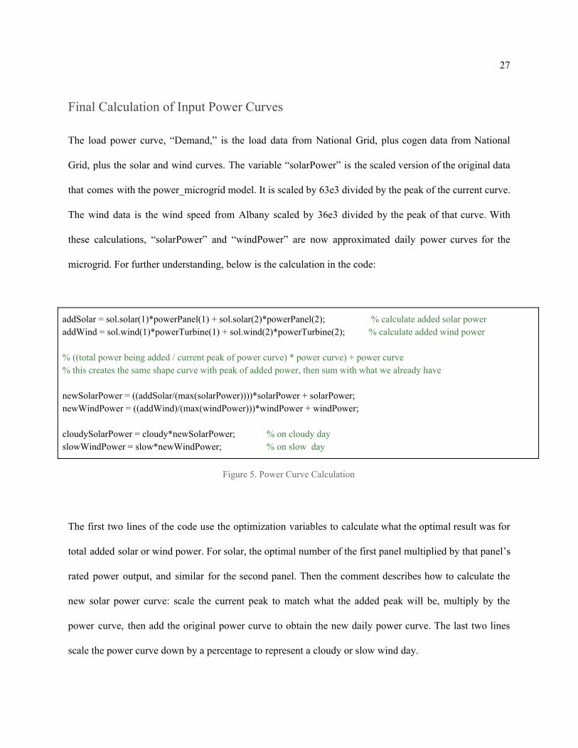
Final Calculation of Input Power Curves

The load power curve, “Demand,” is the load data from National Grid, plus cogen data from National

Grid, plus the solar and wind curves. The variable “solarPower” is the scaled version of the original data

that comes with the power_microgrid model. It is scaled by 63e3 divided by the peak of the current curve.

The wind data is the wind speed from Albany scaled by 36e3 divided by the peak of that curve. With

these calculations, “solarPower” and “windPower” are now approximated daily power curves for the

microgrid. For further understanding, below is the calculation in the code:

addSolar = sol.solar(1)*powerPanel(1) + sol.solar(2)*powerPanel(2); % calculate added solar power addWind = sol.wind(1)*powerTurbine(1) + sol.wind(2)*powerTurbine(2); % calculate added wind power % ((total power being added / current peak of power curve) * power curve) + power curve % this creates the same shape curve with peak of added power, then sum with what we already have newSolarPower = ((addSolar/(max(solarPower))))*solarPower + solarPower; newWindPower = ((addWind)/(max(windPower)))*windPower + windPower; cloudySolarPower = cloudy*newSolarPower; % on cloudy day slowWindPower = slow*newWindPower; % on slow day

Figure 5. Power Curve Calculation

The first two lines of the code use the optimization variables to calculate what the optimal result was for

total added solar or wind power. For solar, the optimal number of the first panel multiplied by that panel’s

rated power output, and similar for the second panel. Then the comment describes how to calculate the

new solar power curve: scale the current peak to match what the added peak will be, multiply by the

power curve, then add the original power curve to obtain the new daily power curve. The last two lines

scale the power curve down by a percentage to represent a cloudy or slow wind day.

28

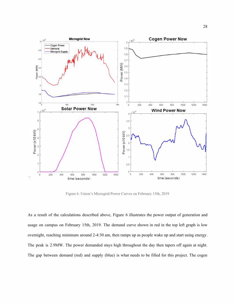
Figure 6. Union’s Microgrid Power Curves on February 15th, 2019

As a result of the calculations described above, Figure 6 illustrates the power output of generation and

usage on campus on February 15th, 2019. The demand curve shown in red in the top left graph is low

overnight, reaching minimum around 2-4:30 am, then ramps up as people wake up and start using energy.

The peak is 2.9MW. The power demanded stays high throughout the day then tapers off again at night.

The gap between demand (red) and supply (blue) is what needs to be filled for this project. The cogen

29

power averages around 1.8MW. The solar power output is only high during the solar day, while wind

power varies based on wind speed.

MATLAB Code Design

The final code is in Appendix A-D. It is thoroughly commented to explain the variables, steps, equations,

and verifications. In this section, I will discuss the flow of the code. First, the optimization toolbox is used

to set up the optimization problem, the variables of generation systems and their sizes and costs, and some

initial constraints.

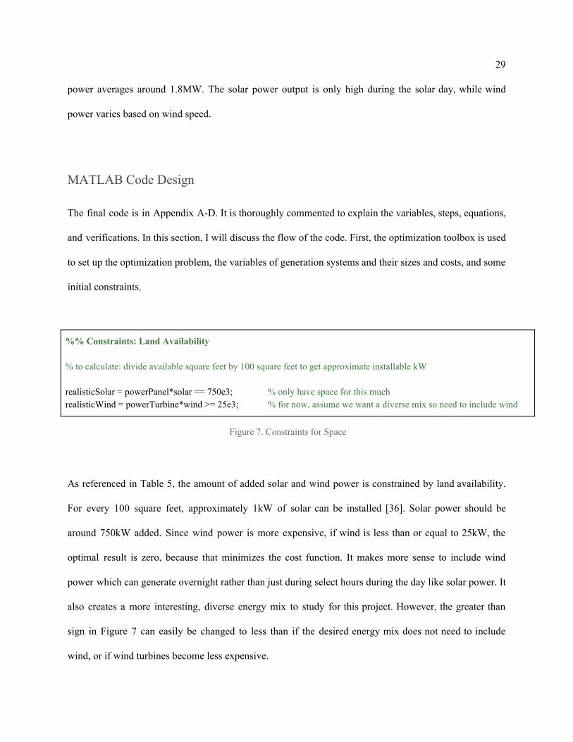
%% Constraints: Land Availability % to calculate: divide available square feet by 100 square feet to get approximate installable kW realisticSolar = powerPanel*solar == 750e3; % only have space for this much realisticWind = powerTurbine*wind >= 25e3; % for now, assume we want a diverse mix so need to include wind

Figure 7. Constraints for Space

As referenced in Table 5, the amount of added solar and wind power is constrained by land availability.

For every 100 square feet, approximately 1kW of solar can be installed [36]. Solar power should be

around 750kW added. Since wind power is more expensive, if wind is less than or equal to 25kW, the

optimal result is zero, because that minimizes the cost function. It makes more sense to include wind

power which can generate overnight rather than just during select hours during the day like solar power. It

also creates a more interesting, diverse energy mix to study for this project. However, the greater than

sign in Figure 7 can easily be changed to less than if the desired energy mix does not need to include

wind, or if wind turbines become less expensive.

30

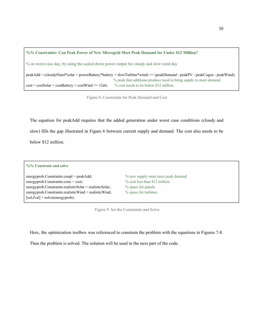
%% Constraints: Can Peak Power of New Microgrid Meet Peak Demand for Under $12 Million? % on worst case day, by using the scaled down power output for cloudy and slow wind day peakAdd = (cloudyPanel*solar + powerBattery*battery + slowTurbine*wind) >= (peakDemand - peakPV - peakCogen - peakWind); % peak that additions produce need to bring supply to meet demand cost = costSolar + costBattery + costWind <= 12e6; % cost needs to be below $12 million

Figure 8. Constraints for Peak Demand and Cost

The equation for peakAdd requires that the added generation under worst case conditions (cloudy and

slow) fills the gap illustrated in Figure 6 between current supply and demand. The cost also needs to be

below $12 million.

%% Constrain and solve energyprob.Constraints.conpl = peakAdd; % new supply must meet peak demand energyprob.Constraints.conc = cost; % cost less than $12 million energyprob.Constraints.realisticSolar = realisticSolar; % space for panels energyprob.Constraints.realisticWind = realisticWind; % space for turbines [sol,fval] = solve(energyprob);

Figure 9. Set the Constraints and Solve

Here, the optimization toolbox was referenced to constrain the problem with the equations in Figures 7-8.

Then the problem is solved. The solution will be used in the next part of the code.

31

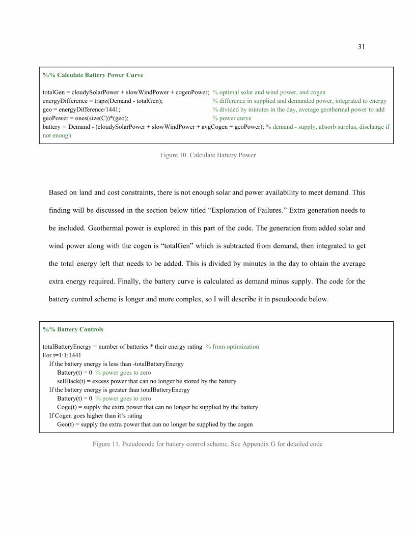
%% Calculate Battery Power Curve totalGen = cloudySolarPower + slowWindPower + cogenPower; % optimal solar and wind power, and cogen energyDifference = trapz(Demand - totalGen); % difference in supplied and demanded power, integrated to energy geo = energyDifference/1441; % divided by minutes in the day, average geothermal power to add geoPower = ones(size(C))*(geo); % power curve battery = Demand - (cloudySolarPower + slowWindPower + avgCogen + geoPower); % demand - supply, absorb surplus, discharge if not enough

Figure 10. Calculate Battery Power

Based on land and cost constraints, there is not enough solar and power availability to meet demand. This

finding will be discussed in the section below titled “Exploration of Failures.” Extra generation needs to

be included. Geothermal power is explored in this part of the code. The generation from added solar and

wind power along with the cogen is “totalGen” which is subtracted from demand, then integrated to get

the total energy left that needs to be added. This is divided by minutes in the day to obtain the average

extra energy required. Finally, the battery curve is calculated as demand minus supply. The code for the

battery control scheme is longer and more complex, so I will describe it in pseudocode below.

%% Battery Controls totalBatteryEnergy = number of batteries * their energy rating % from optimization For t=1:1:1441 If the battery energy is less than -totalBatteryEnergy Battery(t) = 0 % power goes to zero sellBack(t) = excess power that can no longer be stored by the battery If the battery energy is greater than totalBatteryEnergy Battery(t) = 0 % power goes to zero Coge(t) = supply the extra power that can no longer be supplied by the battery If Cogen goes higher than it’s rating Geo(t) = supply the extra power that can no longer be supplied by the cogen

Figure 11. Pseudocode for battery control scheme. See Appendix G for detailed code

32

Figure 11 describes the simplified flow of the control scheme. If the energy mix supplies more than

demanded, excess is stored because the difference would be negative. If demand is higher than supply, the

battery will discharge and supply the rest. However, this is limited by the amount of energy that the

battery can store. Similarly, it can only discharge what it has already stored.

Simulink Model Design

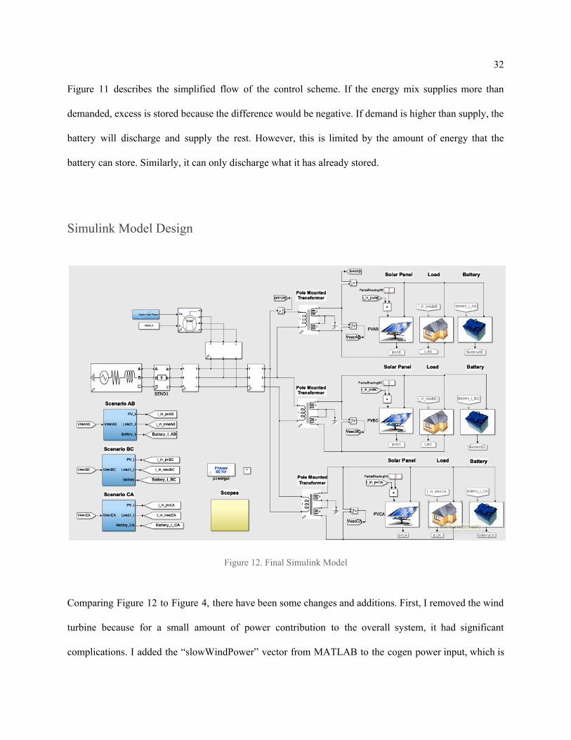
Figure 12. Final Simulink Model

Comparing Figure 12 to Figure 4, there have been some changes and additions. First, I removed the wind

turbine because for a small amount of power contribution to the overall system, it had significant

complications. I added the “slowWindPower” vector from MATLAB to the cogen power input, which is

33

now the subsystem to the left of the cogen block, described below in Figure 14. Also as part of the cogen

power input is the geothermal power for simplicity. I removed the RLC load in Figure 4 because I found

it was unnecessary. I added three phase power measurement blocks and removed some of the unused

meters. Lastly, I added the battery to each phase. The solar photovoltaic block, load block, and battery

block each have current inputs that are calculated in the scenario blocks. For a look inside these blocks

refer to Appendix E.

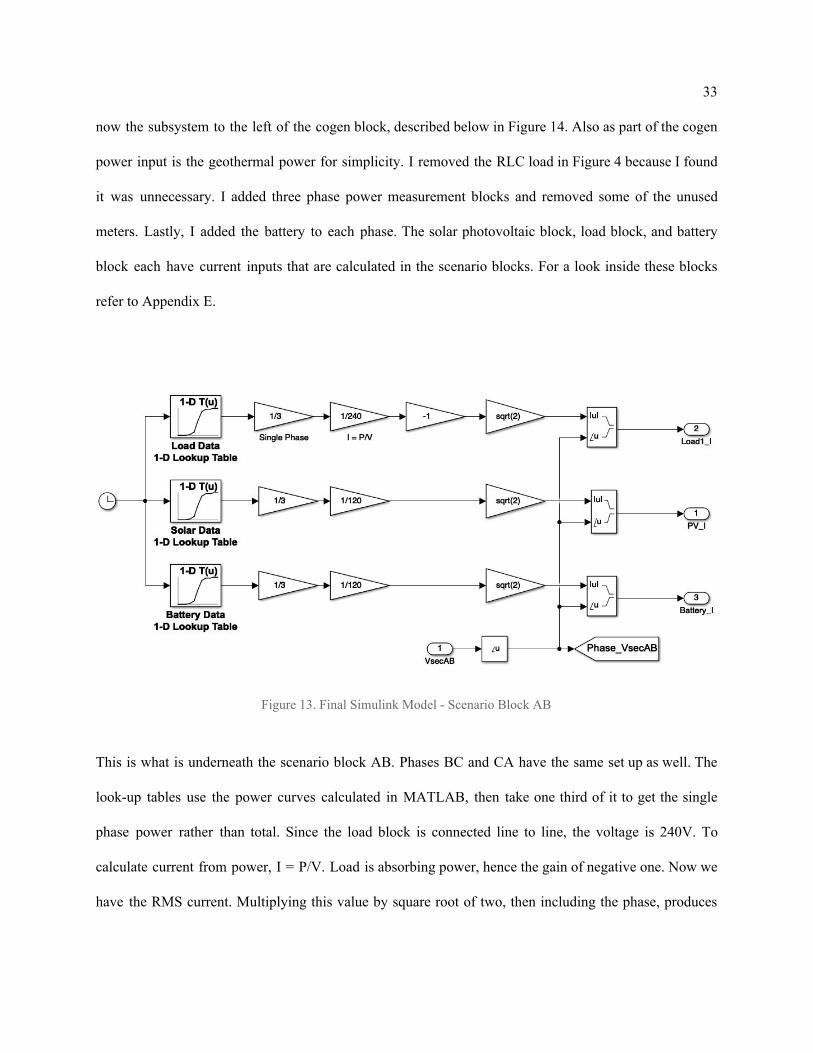
Figure 13. Final Simulink Model - Scenario Block AB

This is what is underneath the scenario block AB. Phases BC and CA have the same set up as well. The

look-up tables use the power curves calculated in MATLAB, then take one third of it to get the single

phase power rather than total. Since the load block is connected line to line, the voltage is 240V. To

calculate current from power, I = P/V. Load is absorbing power, hence the gain of negative one. Now we

have the RMS current. Multiplying this value by square root of two, then including the phase, produces

34

the current to input into the load block. Since the solar panel and battery are line to ground, the voltage to

divide by is only 120V.

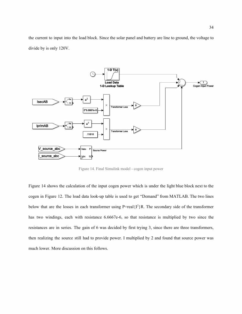
Figure 14. Final Simulink model - cogen input power

Figure 14 shows the calculation of the input cogen power which is under the light blue block next to the

cogen in Figure 12. The load data look-up table is used to get “Demand” from MATLAB. The two lines

below that are the losses in each transformer using P=real{I2}R. The secondary side of the transformer

has two windings, each with resistance 6.6667e-6, so that resistance is multiplied by two since the

resistances are in series. The gain of 6 was decided by first trying 3, since there are three transformers,

then realizing the source still had to provide power. I multiplied by 2 and found that source power was

much lower. More discussion on this follows.

35

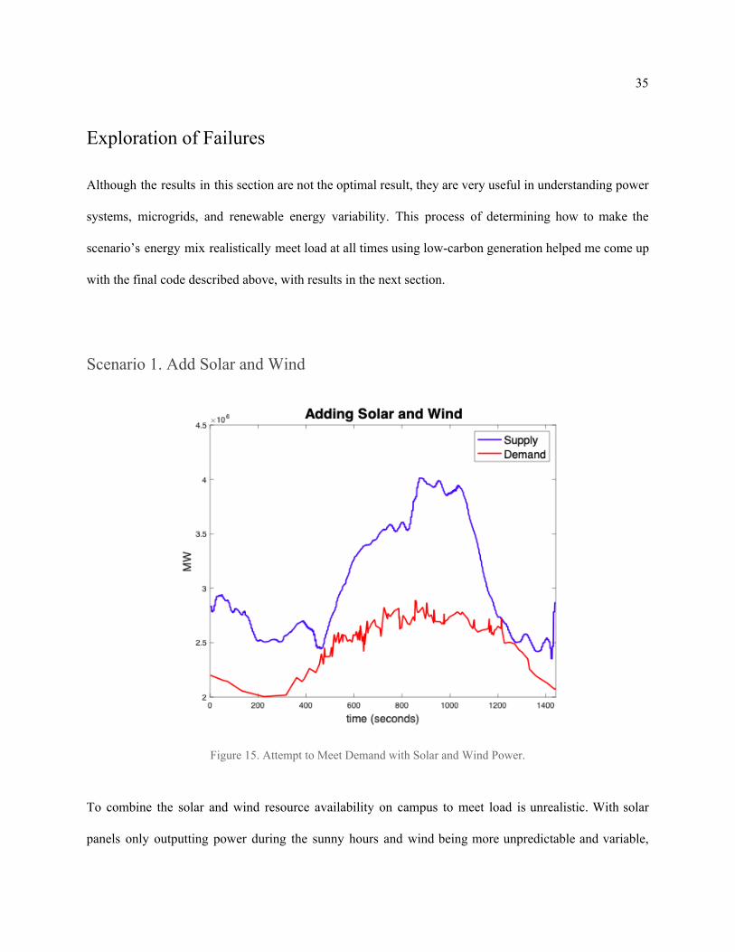
Exploration of Failures

Although the results in this section are not the optimal result, they are very useful in understanding power

systems, microgrids, and renewable energy variability. This process of determining how to make the

scenario’s energy mix realistically meet load at all times using low-carbon generation helped me come up

with the final code described above, with results in the next section.

Scenario 1. Add Solar and Wind

Figure 15. Attempt to Meet Demand with Solar and Wind Power.

To combine the solar and wind resource availability on campus to meet load is unrealistic. With solar

panels only outputting power during the sunny hours and wind being more unpredictable and variable,

36

this would not make a very reliable energy mix. Union would have to plan to overinstall panels and

turbines, resulting in very high expenses. This scenario’s “optimal” result was adding 40 5kW and 79

20kW wind turbines with 1100kW of solar PV to meet load under worst case conditions. Adding 1780kW

of wind power is not reasonable, due to noise and land constraints. The total cost of this system is only

$4,231,000. However, this scenario is not currently worth any more investigation.

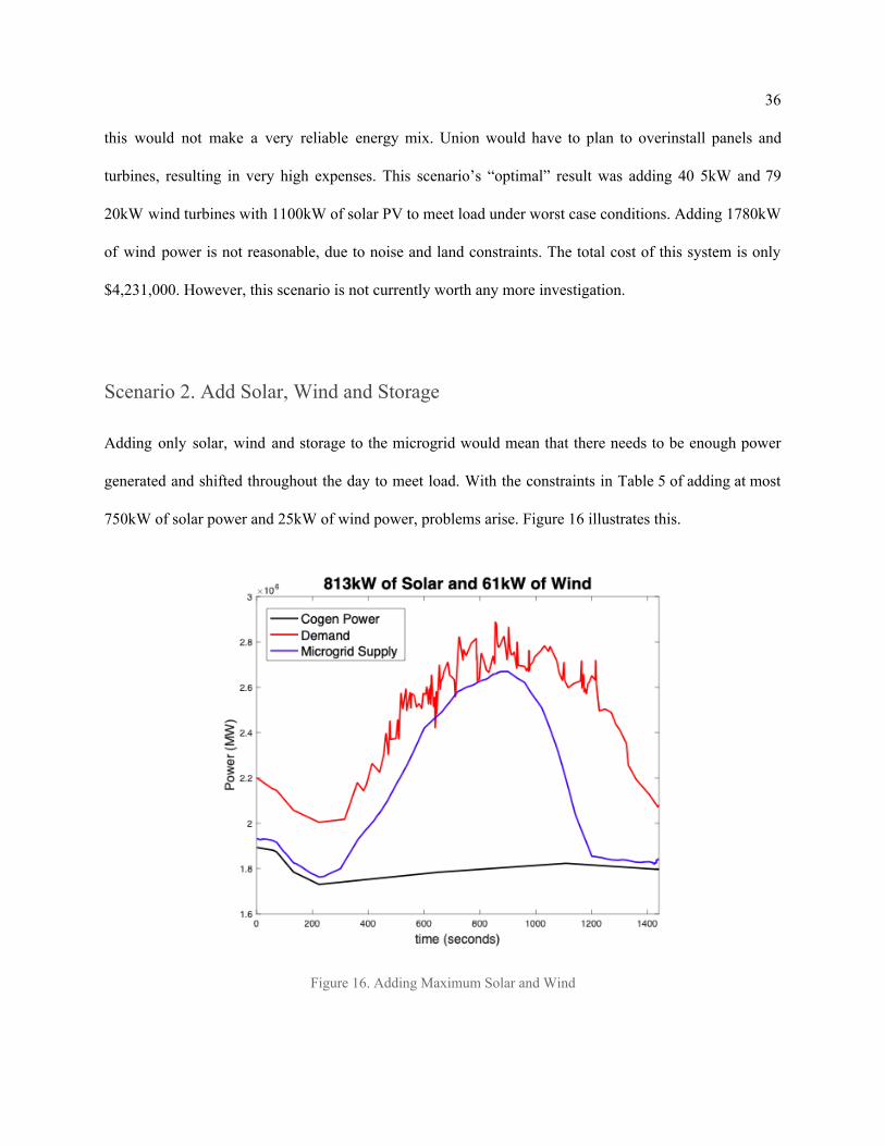
Scenario 2. Add Solar, Wind and Storage

Adding only solar, wind and storage to the microgrid would mean that there needs to be enough power

generated and shifted throughout the day to meet load. With the constraints in Table 5 of adding at most

750kW of solar power and 25kW of wind power, problems arise. Figure 16 illustrates this.

Figure 16. Adding Maximum Solar and Wind

37

Adding the maximum amount of solar and wind power, 750kW and 25kW respectively, is not enough to

meet demand. There is never any significant surplus power. Hence, adding battery storage would not help

because it would never have any energy to charge or discharge. Therefore, Union’s microgrid needs to

add more generation.

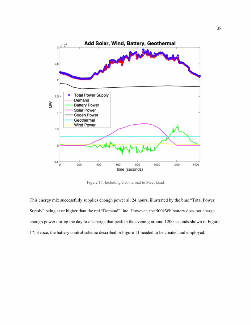
Scenario 3. Add Solar, Storage and Low-Carbon Generation

This scenario will simulate adding the maximum solar and wind power plus battery storage in order to

determine how much extra power the microgrid would be required to produce to meet load. It is notable

that the extra generation does not necessarily have to ramp up and down to complement solar and wind

power curves. Rather, it could stay at a constant rate and any excess power could be stored and shifted to

the evening peaking need.

38

Figure 17. Including Geothermal to Meet Load

This energy mix successfully supplies enough power all 24 hours, illustrated by the blue “Total Power

Supply” being at or higher than the red “Demand” line. However, the 500kWh battery does not charge

enough power during the day to discharge that peak in the evening around 1200 seconds shown in Figure

17. Hence, the battery control scheme described in Figure 11 needed to be created and employed.

39

Final Result: Optimal Energy Mix

Scenario 3 Continued.

To make this scenario realistic, the battery can only discharge what it has already charged from excess

power on the microgrid. Since there are already limits on the amount of PV and wind power to

implement, the amount of baseload geothermal and batteries needs to be altered in order to provide

enough power throughout the day, complementing the variable generation. Another change in this

scenario is slightly increasing the cogen to 2MW power production throughout the day. Currently, Union

has a contract to buy a specified amount of power from National Grid at all times, so the cogen varies

based on that. For example, if the demand is 2MW after considering the wind and solar power supplied,

and Union is required to buy 50kW from National Grid, the cogen only should produce the difference.

Once Union demonstrates the ability to generate enough power to meet load, the requirement of buying a

certain amount of power will be removed.

40

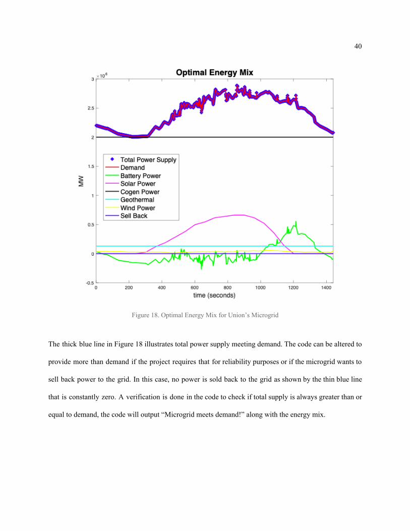
Figure 18. Optimal Energy Mix for Union’s Microgrid

The thick blue line in Figure 18 illustrates total power supply meeting demand. The code can be altered to

provide more than demand if the project requires that for reliability purposes or if the microgrid wants to

sell back power to the grid. In this case, no power is sold back to the grid as shown by the thin blue line

that is constantly zero. A verification is done in the code to check if total supply is always greater than or

equal to demand, the code will output “Microgrid meets demand!” along with the energy mix.

41

Figure 19. Output of MATLAB program describing the optimal energy mix

Figure 19 lists the energy generation and storage sources determined optimal by this program. It includes

the maximum added solar and wind power, slightly increasing the cogen’s output to 2MW, adding 130kW

of geothermal, and 4.5MWh of lithium ion battery storage. This result will be analyzed in the following

discussion session, after a summary of these findings.

42

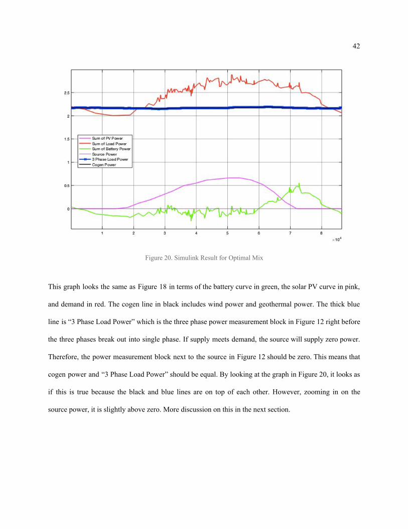
Figure 20. Simulink Result for Optimal Mix

This graph looks the same as Figure 18 in terms of the battery curve in green, the solar PV curve in pink,

and demand in red. The cogen line in black includes wind power and geothermal power. The thick blue

line is “3 Phase Load Power” which is the three phase power measurement block in Figure 12 right before

the three phases break out into single phase. If supply meets demand, the source will supply zero power.

Therefore, the power measurement block next to the source in Figure 12 should be zero. This means that

cogen power and “3 Phase Load Power” should be equal. By looking at the graph in Figure 20, it looks as

if this is true because the black and blue lines are on top of each other. However, zooming in on the

source power, it is slightly above zero. More discussion on this in the next section.

43

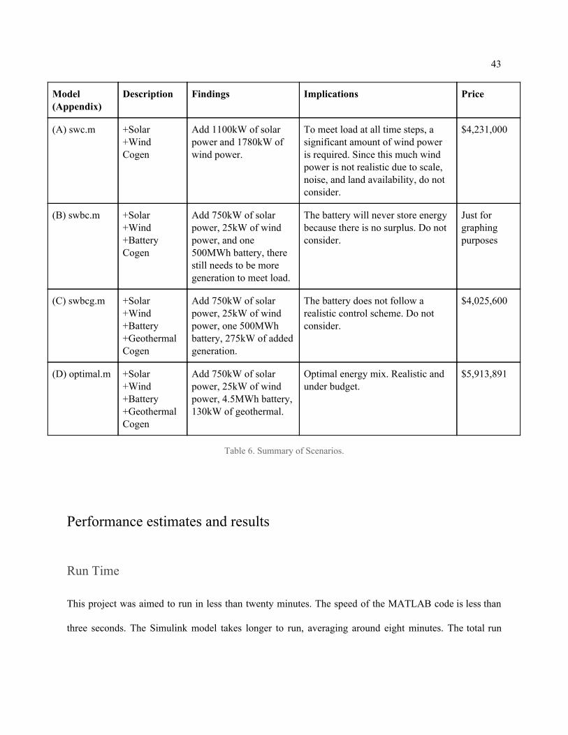
Model (Appendix)

Description Findings Implications Price

(A) swc.m

+Solar +Wind Cogen

Add 1100kW of solar power and 1780kW of wind power.

To meet load at all time steps, a significant amount of wind power is required. Since this much wind power is not realistic due to scale, noise, and land availability, do not consider.

$4,231,000

(B) swbc.m +Solar +Wind +Battery Cogen

Add 750kW of solar power, 25kW of wind power, and one 500MWh battery, there still needs to be more generation to meet load.

The battery will never store energy because there is no surplus. Do not consider.

Just for graphing purposes

(C) swbcg.m +Solar +Wind +Battery +Geothermal Cogen

Add 750kW of solar power, 25kW of wind power, one 500MWh battery, 275kW of added generation.

The battery does not follow a realistic control scheme. Do not consider.

$4,025,600

(D) optimal.m +Solar +Wind +Battery +Geothermal Cogen

Add 750kW of solar power, 25kW of wind power, 4.5MWh battery, 130kW of geothermal.

Optimal energy mix. Realistic and under budget.

$5,913,891

Table 6. Summary of Scenarios.

Performance estimates and results

Run Time

This project was aimed to run in less than twenty minutes. The speed of the MATLAB code is less than

three seconds. The Simulink model takes longer to run, averaging around eight minutes. The total run

44

time is under the time constraint. The Simulink speed could be improved by simplifying the model or

researching ways to increase the speed. I already lowered the relative tolerance and increased the step size

to increase speed. The MATLAB program could even be improved by changing the structure of the loops

to increase speed if desired.

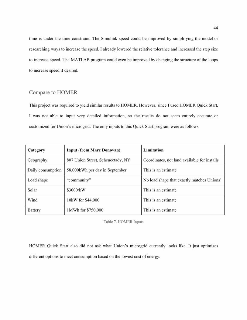
Compare to HOMER

This project was required to yield similar results to HOMER. However, since I used HOMER Quick Start,

I was not able to input very detailed information, so the results do not seem entirely accurate or

customized for Union’s microgrid. The only inputs to this Quick Start program were as follows:

Category Input (from Marc Donovan) Limitation

Geography 807 Union Street, Schenectady, NY Coordinates, not land available for installs

Daily consumption 58,000kWh per day in September This is an estimate

Load shape “community” No load shape that exactly matches Unions’

Solar $3000/kW This is an estimate

Wind 10kW for $44,000 This is an estimate

Battery 1MWh for $750,000 This is an estimate

Table 7. HOMER Inputs

HOMER Quick Start also did not ask what Union’s microgrid currently looks like. It just optimizes

different options to meet consumption based on the lowest cost of energy.

45

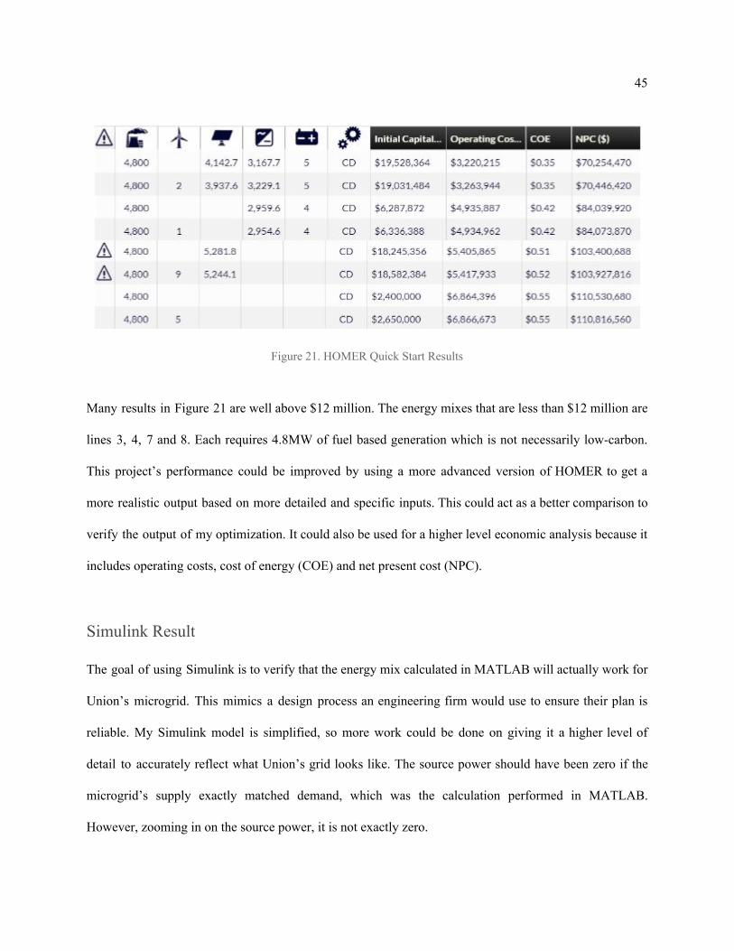
Figure 21. HOMER Quick Start Results

Many results in Figure 21 are well above $12 million. The energy mixes that are less than $12 million are

lines 3, 4, 7 and 8. Each requires 4.8MW of fuel based generation which is not necessarily low-carbon.

This project’s performance could be improved by using a more advanced version of HOMER to get a

more realistic output based on more detailed and specific inputs. This could act as a better comparison to

verify the output of my optimization. It could also be used for a higher level economic analysis because it

includes operating costs, cost of energy (COE) and net present cost (NPC).

Simulink Result

The goal of using Simulink is to verify that the energy mix calculated in MATLAB will actually work for

Union’s microgrid. This mimics a design process an engineering firm would use to ensure their plan is

reliable. My Simulink model is simplified, so more work could be done on giving it a higher level of

detail to accurately reflect what Union’s grid looks like. The source power should have been zero if the

microgrid’s supply exactly matched demand, which was the calculation performed in MATLAB.

However, zooming in on the source power, it is not exactly zero.

46

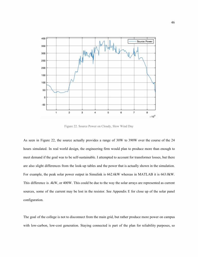
Figure 22. Source Power on Cloudy, Slow Wind Day

As seen in Figure 22, the source actually provides a range of 30W to 390W over the course of the 24

hours simulated. In real world design, the engineering firm would plan to produce more than enough to

meet demand if the goal was to be self-sustainable. I attempted to account for transformer losses, but there

are also slight differences from the look-up tables and the power that is actually shown in the simulation.

For example, the peak solar power output in Simulink is 662.6kW whereas in MATLAB it is 663.0kW.

This difference is .4kW, or 400W. This could be due to the way the solar arrays are represented as current

sources, some of the current may be lost in the resistor. See Appendix E for close up of the solar panel

configuration.

The goal of the college is not to disconnect from the main grid, but rather produce more power on campus

with low-carbon, low-cost generation. Staying connected is part of the plan for reliability purposes, so

47

drawing 30-380W of power is not an issue, it is just not part of the goal of this specific project. However,

future work includes making the solar arrays in Simulink actually output the amount specified in

MATLAB to prove that supply meets demand.

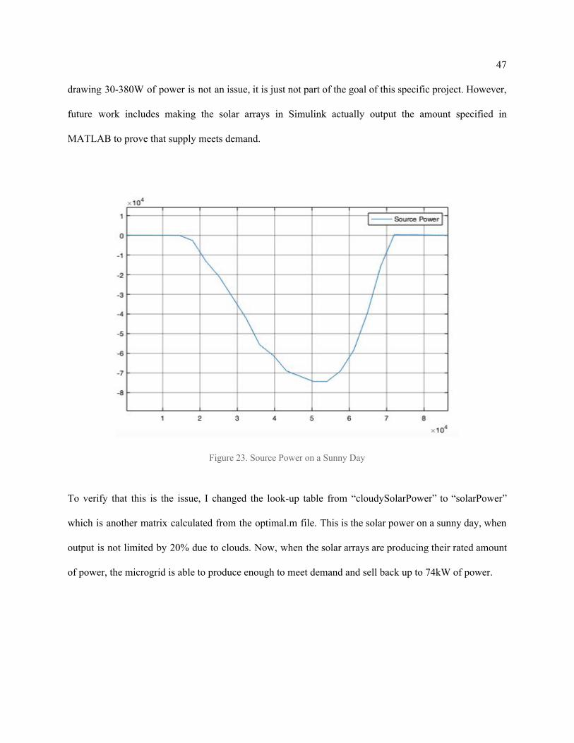
Figure 23. Source Power on a Sunny Day

To verify that this is the issue, I changed the look-up table from “cloudySolarPower” to “solarPower”

which is another matrix calculated from the optimal.m file. This is the solar power on a sunny day, when

output is not limited by 20% due to clouds. Now, when the solar arrays are producing their rated amount

of power, the microgrid is able to produce enough to meet demand and sell back up to 74kW of power.

48

Cost

I did not apply for a research grant, because the estimated cost was zero. This entire project did not cost

anything since it was all done on my computer, meeting the intended cost. I have MATLAB provided

with Union College’s license, but if I did not have this access it would cost $49 for students or $150 for

home use [37]. HOMER Quick Start is free, but a more advanced version is $65 per month [31].

User-friendly Code

The MATLAB code package is fairly easy to use (see User’s Manual). The user can edit the inputs to

match their power requirements and power curves to see the optimal low-carbon, least cost energy mix to

meet their load. It is worth noting that the point of this project was to determine this energy mix for

Union’s microgrid, not make a program for others to do the same, so importance was placed on the design

specific to Union’s microgrid.

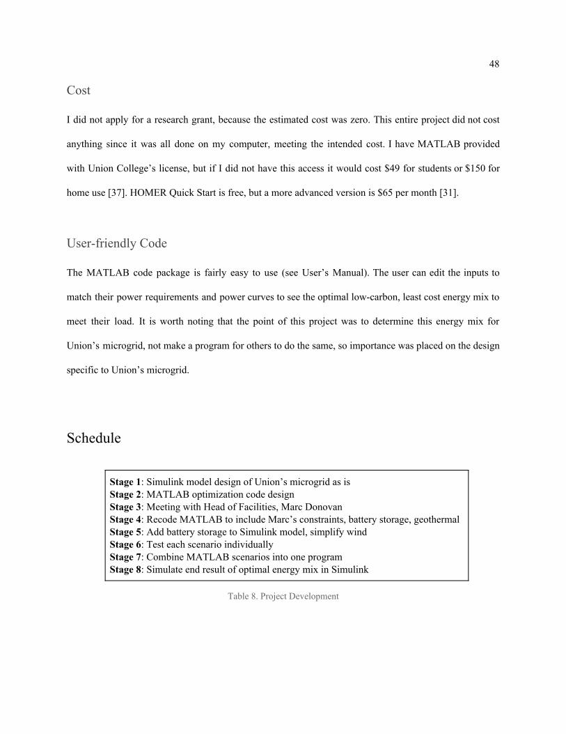
Schedule

Stage 1: Simulink model design of Union’s microgrid as is Stage 2: MATLAB optimization code design Stage 3: Meeting with Head of Facilities, Marc Donovan Stage 4: Recode MATLAB to include Marc’s constraints, battery storage, geothermal Stage 5: Add battery storage to Simulink model, simplify wind Stage 6: Test each scenario individually Stage 7: Combine MATLAB scenarios into one program Stage 8: Simulate end result of optimal energy mix in Simulink

Table 8. Project Development

49

Reflecting on my terms of working on this project, I would have focused on the MATLAB optimization

code first. I spent most of my time trying to get the Simulink model to work, when the optimization could

have occurred without it, since it just provided modelling of the results for verification. I also would have

met with Marc Donovan earlier to understand the constraints before I began coding and designing. He has

been extremely busy and is hard to get in touch with, so I did my best. However, I definitely learned the

importance of talking with the stakeholders early in project development.

User’s Manual

You must have MATLAB 2019B installed on your computer. First, email mcmahonc@union.edu or visit

https://muse.union.edu/2020capstone-mcmahonc/capstone-project/final-project/ to get the program files.

Download, save, and open in MATLAB. The beginning of optimal.m describes each variable and power

curve, so that you can input the specific numbers for your system. If you want to input specific power

curves, use MATLAB’s “import data” tool to import your data in vector form from an excel file. Rename

it Demand for load data, solarPower for solar power, windPower for wind power data, cogenPower for

slightly varying power, geoPower for baseload types of generation, and battery for battery

charge/discharge. Or, you may scale the curves to match your peak values, as I mentioned above in Figure

5. To view what the curves look like, right click on the variable in the workspace and click plot. Once you

are satisfied with the data inputs, include your options for size and cost of solar, wind, and battery

systems. Then edit the baseline peaks to match what your system currently has. Next, understand the

constraints, which are broken into sections for readability. Determine if there are land constraints by using

the equation in that section to calculate the amount of solar and wind power you can have. Then edit the

maximum total cost. Change the values of “cloudy” and “slow” to alter the effect of a cloudy or slow

50

wind speed day. Increase or decrease “number” and “powerCogen” to change the number of batteries and

power output of the cogen, respectively. Finally, click run and view the plot and description of the

resulting energy mix along with the total cost.

If the output is [], this means that there is no solution to your optimization problem. You will need to

troubleshoot and determine why no solution can be found. Perhaps you are asking for too much

generation, but constraining it so that it can never reach that amount. Or your desired energy mix is made

up of generation that cannot meet demand at certain times. Viewing the output plots should help you

determine what went wrong.

The outputs of the MATLAB code are the inputs to the Simulink model. See this by clicking on one

scenario, AB for example, then clicking the look-up table for load, solar, or battery. The vector from

MATLAB will be listed there. Navigate to the Modelling tab at the top of the screen, then Model Settings

drop-down menu, click Model Properties, then CallBack. This should be listed there:

load('input_data.mat'). Next, run the model. Expect it to take 5-10 minutes. View the plots by clicking the

scopes block on the main page. If you want to change the shading factor in Simulink, in addition to

scaling down by 20% which was done in MATLAB, then click the partial shading block above each of

the solar panels.

Discussion, Conclusions, and Recommendations

The goal of this project is to determine a low-cost, low-carbon energy mix that realistically and reliably

meets Union’s load on the peak day under worst case conditions. I created a program in MATLAB that

51

uses the linear programming method of optimization within the optimization toolbox. The codes can be

found in Appendices A-D. Realistic constraints were a crucial part of calculating the energy mix, such as

land availability, cost and peaking constraints. Meeting with the Head of Facilities at Union, Marc

Donovan, allowed me to get specific numbers for these constraints. The maximum amount of solar power

being added is 750kW, and wind is not really being considered, but geothermal power is. Geothermal has

the benefit of being renewable but not variable like solar and wind. For my project, I did include wind to

make the mix more diverse. However, this could easily be removed from the code. The “reliable”

requirement means that the energy mix can produce enough supply to meet the highest demand on the

worst case day, meaning a cloudy and slow wind speed day. National Grid data was used for the peak

demand day. In MATLAB, the energy mix calculated successfully supplies enough power to meet

demand even with solar and wind power outputs limited by 20 percent. The cost of additions is under $6

million, less than half of the maximum budget. The resulting generation includes solar, wind, geothermal,

and lithium ion battery storage.

The next part of my project was to simulate this energy mix in the model of Union’s microgrid in

Simulink. I interpreted the plots to determine the performance of the energy mix. The source power

should be zero if supply met demand, but the source supplied 30-390 Watts of power. This is very

minimal, and is attributed to the slight difference in solar power output in MATLAB to Simulink. It could

also be due to other minor losses on the grid. When the 20 percent loss of output power was removed

from the simulation, the microgrid supplied more than enough to meet demand and was able to sell some

power back to the grid. The 30-390 Watts is negligible for now, but if Union were to consider this energy

mix, more complex simulations would be done to come up with an energy mix that draws zero power if

that is the goal. Since this energy mix came in under-budget, Union could add more geothermal power

generation to produce more than demand even on the worst case day. This could be retested in the

52

Simulink model to verify that the source power is zero, or below zero meaning we are able to sell power

back to the grid.

This project can be improved by using actual solar and wind data. Instead of scaling it down by 20

percent, more analysis could be done to determine if it is better to find a cloudy day and use that data, or

scale the power curve down by a specific amount as I did. The Simulink model could also be improved by

creating a battery control scheme rather than calculating the current from the power curve in MATLAB.

This would just validate that the model works properly. More research could be done into battery control

schemes, and how accurate the one employed in the MATLAB code is. The economics of increasing the

cogen to 2MW versus keeping it where it is, averaging around 1.8MW, and just adding more geothermal

could be analyzed. Long term costs would be interesting to explore and see after 10 years which energy

mix is the best in terms of cost. The contract Union has with National Grid and how it could potentially

change based on our generation could factor into cost and possibly constrain the system. More detailed

analysis of placement of panels and turbines and their resulting energy production would be required

before any serious plans could be made. As previously stated, advanced versions of HOMER should be

used to check the validity of this project’s result. A more complex Simulink model could be built from the

one I designed to more accurately reflect Union’s grid. Lastly, any steps taking this project further should

be advised by Marc Donovan and Professor Dosiek.

This senior capstone project has allowed me to learn in depth about power flow, balanced loads,

renewable generation, microgrid control schemes, optimization through linear programming, and

Simulink modelling. I also came to appreciate the power of putting pen to paper and sketching out goals,

system design, or troubleshooting. Specifically in Simulink, this project involved an intense amount of

troubleshooting. I created over twenty different models of Union’s microgrid, each with different levels of

53

detail and types of control schemes in hopes of getting it right. I calculated power, currents, and voltages

to make sense of the issues in each model. I used simple control schemes and more complex PI

controllers. Professor Dosiek helped me realize that transformer losses needed to be accounted for. Since

the models took anywhere from five to twenty minutes to run, troubleshooting over and over took a

significant amount of time, patience, and research. Finishing this project and feeling proud of all that I

have learned is a great reward.

54

References

[1] C. Milan, C. Bojesen and M. Nielsen, "A cost optimization model for 100% renewable residential energy supply systems", Energy, vol. 48, no. 1, pp. 118-127, 2012. Available: 10.1016/j.energy.2012.05.034. [2] "Curtailment Fast Facts", Caiso.com, 2019. [Online]. Available: https://www.caiso.com/Documents/CurtailmentFastFacts.pdf. [Accessed: 22- Nov- 2019]. [3 ]E. Silveira, T. de Oliveira and A. Junior, "Hybrid Energy Scenarios for Fernando de Noronha archipelago", Energy Procedia, vol. 75, pp. 2833-2838, 2015. Available: 10.1016/j.egypro.2015.07.564. [4] E. Alegria, T. Brown, E. Minear and R. Lasseter, "CERTS Microgrid Demonstration With Large-Scale Energy Storage and Renewable Generation", IEEE Transactions on Smart Grid, vol. 5, no. 2, pp. 937-943, 2014. Available: 10.1109/tsg.2013.2286575. [5] T. Mohn, "Campus microgrids: Opportunities and challenges", IEEE, vol. 2012, 2019. Available: 10.1109/PESGM.2012.6344610 [Accessed 22 November 2019]. [6] "New York Gov. Launches ‘Green New Deal’ With Accelerated Clean Energy Targets", Greentechmedia.com, 2019. [Online]. Available: https://www.greentechmedia.com/articles/read/new-york-cuomo-green-new-deal-clean-energy. [Accessed: 22- Nov- 2019]. [7] H. Ringkjøb, P. Haugan and I. Solbrekke, "A review of modelling tools for energy and electricity systems with large shares of variable renewables", Renewable and Sustainable Energy Reviews, vol. 96, pp. 440-459, 2018. Available: 10.1016/j.rser.2018.08.002. [8] Q. Fu et al., "Microgrid Generation Capacity Design With Renewables and Energy Storage Addressing Power Quality and Surety", IEEE Transactions on Smart Grid, vol. 3, no. 4, pp. 2019-2027, 2012. Available: 10.1109/tsg.2012.2223245. [9] "5kW Wind Turbine by Windspire", Windspireenergy.com, 2019. [Online]. Available: https://www.windspireenergy.com/5kW-wind-turbine.htm. [Accessed: 22- Nov- 2019]. [10] E. Hittinger and I. Azevedo, "Bulk Energy Storage Increases United States Electricity System Emissions", Environmental Science & Technology, vol. 49, no. 5, pp. 3203-3210, 2015. Available: 10.1021/es505027p. [11] "The HOMER® Micropower Optimization Model", Nrel.gov, 2019. [Online]. Available: https://www.nrel.gov/docs/fy05osti/37606.pdf. [Accessed: 22- Nov- 2019]. [12] B. Bose, "Global Warming: Energy, Environmental Pollution, and the Impact of Power Electronics", IEEE Industrial Electronics Magazine, vol. 4, no. 1, pp. 6-17, 2010. Available: 10.1109/mie.2010.935860. [13] C. Budischak, D. Sewell, H. Thomson, L. Mach, D. Veron and W. Kempton, "Cost-minimized combinations of wind power, solar power and electrochemical storage, powering the grid up to 99.9% of the time", Journal of Power Sources, vol. 225, pp. 60-74, 2013. Available: 10.1016/j.jpowsour.2012.09.054. [14] R. Srivastava and V. Giri, "Optimization of Hybrid Renewable Resources using HOMER", International Journal of Renewable Energy Research, vol. 6, no. 1, 2016. [Accessed 22 November 2019].

55

[15] J. Lagorse, D. Paire and A. Miraoui, "Sizing optimization of a stand-alone street lighting system powered by a hybrid system using fuel cell, PV and battery", Renewable Energy, vol. 34, no. 3, pp. 683-691, 2009. Available: 10.1016/j.renene.2008.05.030. [16] M. Chaichan, H. Kazem, A. Mahdy and A. Al-Waeely, "Optimal Sizing of a Hybrid System of Renewable Energy for Lighting Street in Salalah-Oman using Homer software", International Journal of Scientific Engineering and Applied Science, vol. 2, no. 5, 2016. [Accessed 22 November 2019]. [17] M. Soshinskaya, W. Crijns-Graus, J. van der Meer and J. Guerrero, "Application of a microgrid with renewables for a water treatment plant", Applied Energy, vol. 134, pp. 20-34, 2014. Available: 10.1016/j.apenergy.2014.07.097. [18] J. Ramos and H. Ramos, "Sustainable application of renewable sources in water pumping systems: Optimized energy system configuration", Energy Policy, vol. 37, no. 2, pp. 633-643, 2009. Available: 10.1016/j.enpol.2008.10.006. [19] Y. Scholz, "Renewable energy based electricity supply at low costs : development of the REMix model and application for Europe", OPUS - Publication Server of the University of Stuttgart, 2012. [Accessed 22 November 2019]. [20] "Union’s CoGen plant – A greener future", Muse.union.edu, 2015. [Online]. Available: https://muse.union.edu/garnetgoesgreen/2015/09/30/unions-cogen-plant-a-greener-future/. [Accessed: 22- Nov- 2019]. [21] “Geothermal energy and the environment - U.S. Energy Information Administration (EIA)", Eia.gov, 2020. [Online]. Available: https://www.eia.gov/energyexplained/geothermal/geothermal-energy-and-the-environment.php. [Accessed: 05- Mar- 2020]. [22] Geothermal FAQs", Energy.gov, 2020. [Online]. Available: https://www.energy.gov/eere/geothermal/geothermal-faqs. [Accessed: 17- Mar- 2020]. [23] "Simplified Model of a Small Scale Micro-Grid- MATLAB & Simulink", Mathworks.com, 2019. [Online]. Available: https://www.mathworks.com/help/physmod/sps/examples/simplified-model-of-a-small-scale-micro-grid.html#d117e28409. [Accessed: 22- Nov- 2019]. [24] "Optimization Problem Types - Mixed-Integer and Constraint Programming", solver, 2019. [Online]. Available: https://www.solver.com/integer-constraint-programming. [Accessed: 22- Nov- 2019]. [25] "Problems Handled by Optimization Toolbox Functions- MATLAB & Simulink", Mathworks.com, 2019. [Online]. Available: https://www.mathworks.com/help/optim/ug/problems-handled-by-optimization-toolbox-functions.html#tblminprobs. [Accessed: 22- Nov- 2019]. [26] "Lightgauge Data Monitoring", Lg878.d.lighthousesolar.com, 2019. [Online]. Available: http://lg878.d.lighthousesolar.com/index.html. [Accessed: 22- Nov- 2019]. [27] L. Tarbi, "How Much Does a 10kW Solar Panel System Cost in 2019? | EnergySage", Solar News, 2019. [Online]. Available: https://news.energysage.com/10kw-solar-systems-compare-prices-installers/. [Accessed: 22- Nov- 2019].

56

[28] "Atlas 3,000-Watt Wind Turbine Generator", Home Depot, 2019. [Online]. Available: https://www.homedepot.com/p/Ramsond-Atlas-3-000-Watt-Wind-Turbine-Generator-LM3500/307565908?mtc=Shopping-B-F_D27E-G-D27E-27_31_CONTROL-Generic-NA-Feed-PLA-NA-NA-CONTROL_Nondoorbells&cm_mmc=Shopping-B-F_D27E-G-D27E-27_31_CONTROL-Generic-NA-Feed-PLA-NA-NA-CONTROL_Nondoorbells-71700000052998923-58700005105045162-92700048675636141&gclid=EAIaIQobChMI493YqYDt5QIVBpSzCh1Zdw_qEAQYASABEgLyIPD_BwE&gclsrc=aw.ds. [Accessed: 22- Nov- 2019]. [29] "Excel 10 - Bergey Windpower Co.", Bergey Windpower Co., 2019. [Online]. Available: http://www.bergey.com/products/grid-tied-turbines/excel-10/. [Accessed: 22- Nov- 2019]. [30] "Excel 10 Off Grid - Bergey Windpower Co.", Bergey Windpower Co., 2019. [Online]. Available: http://www.bergey.com/products/off-grid-turbines/excel-10-off-grid/. [Accessed: 22- Nov- 2019]. [31] "HOMER QuickStart", Quickstart.homerenergy.com, 2019. [Online]. Available: http://quickstart.homerenergy.com/#/app/ee2e61bd-1bb7-47aa-ab2f-c39f78482fef/results/optimization. [Accessed: 22- Nov- 2019]. [32] "COMPARATIVE STUDY OF TECHNOECONOMICS OF LITHIUM-ION AND LEAD-ACID BATTERIES IN MICROGRIDS IN SUB-SAHARAN AFRICA", Nrel.gov, 2019. [Online]. Available: https://www.nrel.gov/docs/fy19osti/73238.pdf. [Accessed: 22- Nov- 2019]. [33] Nrel.gov, 2020. [Online]. Available: https://www.nrel.gov/grid/assets/pdfs/second_grid_sim_fenimore.pdf. [Accessed: 17- Mar- 2020]. [34] "Mixed-Integer Linear Programming Basics: Problem-Based- MATLAB & Simulink", Mathworks.com, 2019. [Online]. Available: https://www.mathworks.com/help/optim/ug/mixed-integer-linear-programming-basics-problem-based.html. [Accessed: 22- Nov- 2019]. [35] Nrel.gov, 2019. [Online]. Available: https://www.nrel.gov/docs/fy19osti/72133.pdf. [Accessed: 17- Mar- 2020]. [36] G. Coast, "Solar Farm Land Requirements: How Much Land Do You Need?", Green Coast, 2019. [Online]. Available: https://greencoast.org/solar-farm-land-requirements/. [Accessed: 17- Mar- 2020]. [37] Mathworks, “Pricing and Licensing”, Mathworks, 2020. [Online]. Available: https://www.mathworks.com/pricing-licensing.html?prodcode=ML&intendeduse=home. [Accessed 17-March-2020].

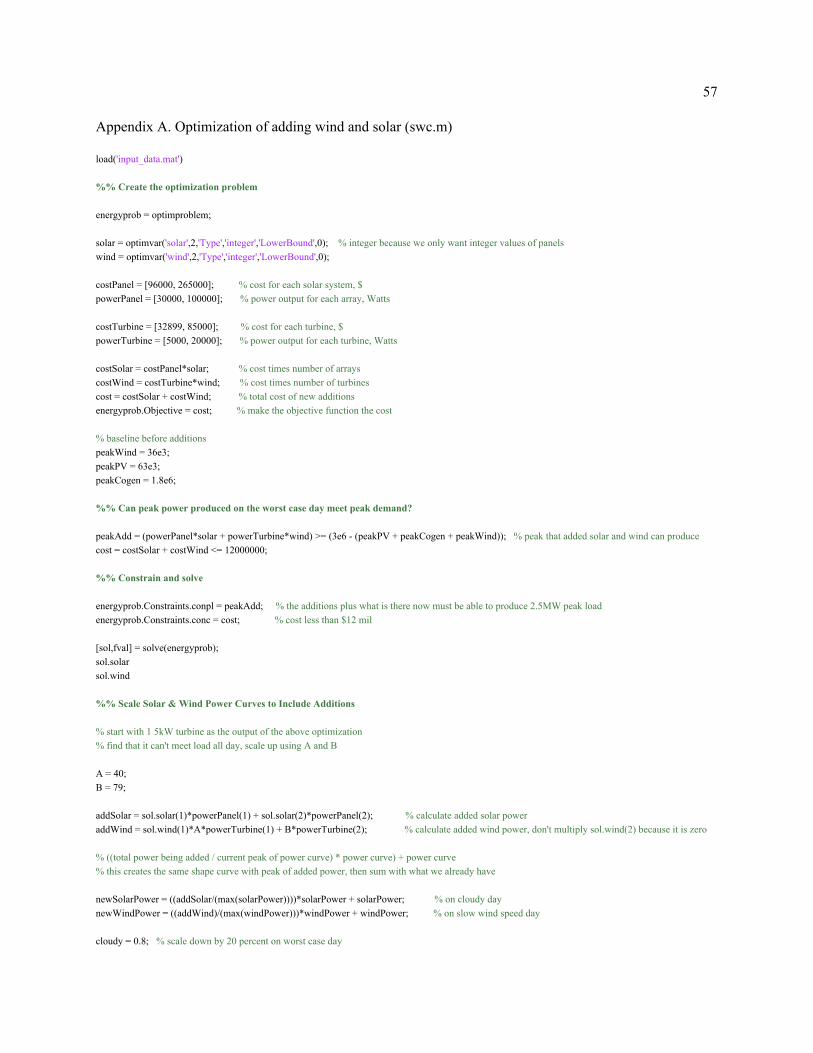
57

Appendix A. Optimization of adding wind and solar (swc.m)

load('input_data.mat') %% Create the optimization problem energyprob = optimproblem; solar = optimvar('solar',2,'Type','integer','LowerBound',0); % integer because we only want integer values of panels wind = optimvar('wind',2,'Type','integer','LowerBound',0); costPanel = [96000, 265000]; % cost for each solar system, $ powerPanel = [30000, 100000]; % power output for each array, Watts costTurbine = [32899, 85000]; % cost for each turbine, $ powerTurbine = [5000, 20000]; % power output for each turbine, Watts costSolar = costPanel*solar; % cost times number of arrays costWind = costTurbine*wind; % cost times number of turbines cost = costSolar + costWind; % total cost of new additions energyprob.Objective = cost; % make the objective function the cost % baseline before additions peakWind = 36e3; peakPV = 63e3; peakCogen = 1.8e6; %% Can peak power produced on the worst case day meet peak demand? peakAdd = (powerPanel*solar + powerTurbine*wind) >= (3e6 - (peakPV + peakCogen + peakWind)); % peak that added solar and wind can produce cost = costSolar + costWind <= 12000000; %% Constrain and solve energyprob.Constraints.conpl = peakAdd; % the additions plus what is there now must be able to produce 2.5MW peak load energyprob.Constraints.conc = cost; % cost less than $12 mil [sol,fval] = solve(energyprob); sol.solar sol.wind %% Scale Solar & Wind Power Curves to Include Additions % start with 1 5kW turbine as the output of the above optimization % find that it can't meet load all day, scale up using A and B A = 40; B = 79; addSolar = sol.solar(1)*powerPanel(1) + sol.solar(2)*powerPanel(2); % calculate added solar power addWind = sol.wind(1)*A*powerTurbine(1) + B*powerTurbine(2); % calculate added wind power, don't multiply sol.wind(2) because it is zero % ((total power being added / current peak of power curve) * power curve) + power curve % this creates the same shape curve with peak of added power, then sum with what we already have newSolarPower = ((addSolar/(max(solarPower))))*solarPower + solarPower; % on cloudy day newWindPower = ((addWind)/(max(windPower)))*windPower + windPower; % on slow wind speed day cloudy = 0.8; % scale down by 20 percent on worst case day

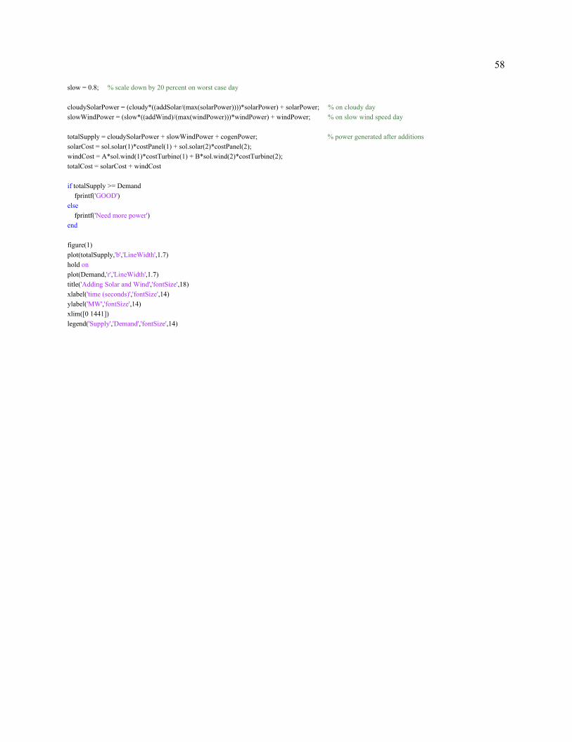
58

slow = 0.8; % scale down by 20 percent on worst case day cloudySolarPower = (cloudy*((addSolar/(max(solarPower))))*solarPower) + solarPower; % on cloudy day slowWindPower = (slow*((addWind)/(max(windPower)))*windPower) + windPower; % on slow wind speed day totalSupply = cloudySolarPower + slowWindPower + cogenPower; % power generated after additions solarCost = sol.solar(1)*costPanel(1) + sol.solar(2)*costPanel(2); windCost = A*sol.wind(1)*costTurbine(1) + B*sol.wind(2)*costTurbine(2); totalCost = solarCost + windCost if totalSupply >= Demand fprintf('GOOD') else fprintf('Need more power') end figure(1) plot(totalSupply,'b','LineWidth',1.7) hold on plot(Demand,'r','LineWidth',1.7) title('Adding Solar and Wind','fontSize',18) xlabel('time (seconds)','fontSize',14) ylabel('MW','fontSize',14) xlim([0 1441]) legend('Supply','Demand','fontSize',14)

59

Appendix B. Optimization of adding wind, solar, battery (swbc.m)

load('input_data.mat') newWindPower = (25e3)/(max(windPower))*windPower + windPower; figure(1) plot(cogenPower,'black','LineWidth',1.7) hold on plot(Demand,'r','LineWidth',1.7) hold on plot(SPD_813+cogenPower+newWindPower,'b','LineWidth',1.7) title('813kW of Solar and 61kW of Wind','fontSize',18) ylabel('Power (MW)','fontSize',14) xlabel('time (seconds)','fontSize',14) xlim([0 1441]) legend('Cogen Power','Demand','Microgrid Supply','fontSize',14)

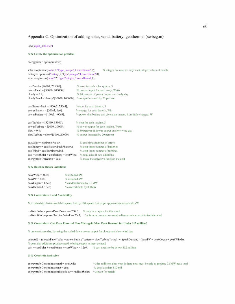
60

Appendix C. Optimization of adding solar, wind, battery, geothermal (swbcg.m)

load('input_data.mat') %% Create the optimization problem energyprob = optimproblem; solar = optimvar('solar',2,'Type','integer','LowerBound',0); % integer because we only want integer values of panels battery = optimvar('battery',2,'Type','integer','LowerBound',0); wind = optimvar('wind',2,'Type','integer','LowerBound',0); costPanel = [96000, 265000]; % cost for each solar system, $ powerPanel = [30000, 100000]; % power output for each array, Watts cloudy = 0.8; % 80 percent of power output on cloudy day cloudyPanel = cloudy*[30000, 100000]; % output lessened by 20 percent costBatteryPack = [400e3, 750e3]; % cost for each battery, $ energyBattery = [500e3, 1e6]; % energy for each battery, Wh powerBattery = [100e3, 400e3]; % power that battery can give at an instant, from fully charged, W costTurbine = [32899, 85000]; % cost for each turbine, $ powerTurbine = [5000, 20000]; % power output for each turbine, Watts slow = 0.8; % 80 percent of power output on slow wind day slowTurbine = slow*[5000, 20000]; % output lessened by 20 percent costSolar = costPanel*solar; % cost times number of arrays costBattery = costBatteryPack*battery; % cost times number of batteries costWind = costTurbine*wind; % cost times number of turbines cost = costSolar + costBattery + costWind; % total cost of new additions energyprob.Objective = cost; % make the objective function the cost %% Baseline Before Additions peakWind = 36e3; % installed kW peakPV = 63e3; % installed kW peakCogen = 1.8e6; % underestimate by 0.1MW peakDemand = 3e6; % overestimate by 0.1MW %% Constraints: Land Availability % to calculate: divide available square feet by 100 square feet to get approximate installable kW realisticSolar = powerPanel*solar == 750e3; % only have space for this much realisticWind = powerTurbine*wind >= 25e3; % for now, assume we want a diverse mix so need to include wind %% Constraints: Can Peak Power of New Microgrid Meet Peak Demand for Under $12 million? % on worst case day, by using the scaled down power output for cloudy and slow wind day peakAdd = (cloudyPanel*solar + powerBattery*battery + slowTurbine*wind) >= (peakDemand - (peakPV + peakCogen + peakWind)); % peak that additions produce need to bring supply to meet demand cost = costSolar + costBattery + costWind <= 12e6; % cost needs to be below $12 million %% Constrain and solve energyprob.Constraints.conpl = peakAdd; % the additions plus what is there now must be able to produce 2.5MW peak load energyprob.Constraints.conc = cost; % cost less than $12 mil energyprob.Constraints.realisticSolar = realisticSolar; % space for panels

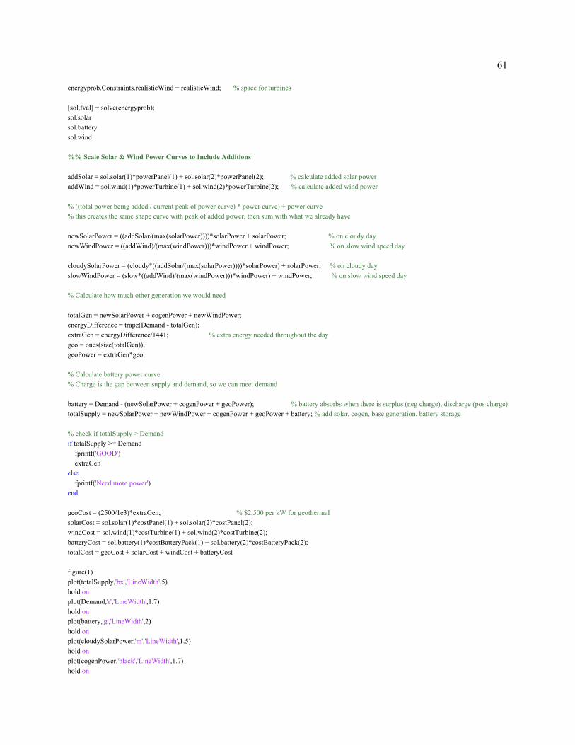
61

energyprob.Constraints.realisticWind = realisticWind; % space for turbines [sol,fval] = solve(energyprob); sol.solar sol.battery sol.wind %% Scale Solar & Wind Power Curves to Include Additions addSolar = sol.solar(1)*powerPanel(1) + sol.solar(2)*powerPanel(2); % calculate added solar power addWind = sol.wind(1)*powerTurbine(1) + sol.wind(2)*powerTurbine(2); % calculate added wind power % ((total power being added / current peak of power curve) * power curve) + power curve % this creates the same shape curve with peak of added power, then sum with what we already have newSolarPower = ((addSolar/(max(solarPower))))*solarPower + solarPower; % on cloudy day newWindPower = ((addWind)/(max(windPower)))*windPower + windPower; % on slow wind speed day cloudySolarPower = (cloudy*((addSolar/(max(solarPower))))*solarPower) + solarPower; % on cloudy day slowWindPower = (slow*((addWind)/(max(windPower)))*windPower) + windPower; % on slow wind speed day % Calculate how much other generation we would need totalGen = newSolarPower + cogenPower + newWindPower; energyDifference = trapz(Demand - totalGen); extraGen = energyDifference/1441; % extra energy needed throughout the day geo = ones(size(totalGen)); geoPower = extraGen*geo; % Calculate battery power curve % Charge is the gap between supply and demand, so we can meet demand battery = Demand - (newSolarPower + cogenPower + geoPower); % battery absorbs when there is surplus (neg charge), discharge (pos charge) totalSupply = newSolarPower + newWindPower + cogenPower + geoPower + battery; % add solar, cogen, base generation, battery storage % check if totalSupply > Demand if totalSupply >= Demand fprintf('GOOD') extraGen else fprintf('Need more power') end geoCost = (2500/1e3)*extraGen; % $2,500 per kW for geothermal solarCost = sol.solar(1)*costPanel(1) + sol.solar(2)*costPanel(2); windCost = sol.wind(1)*costTurbine(1) + sol.wind(2)*costTurbine(2); batteryCost = sol.battery(1)*costBatteryPack(1) + sol.battery(2)*costBatteryPack(2); totalCost = geoCost + solarCost + windCost + batteryCost figure(1) plot(totalSupply,'bx','LineWidth',5) hold on plot(Demand,'r','LineWidth',1.7) hold on plot(battery,'g','LineWidth',2) hold on plot(cloudySolarPower,'m','LineWidth',1.5) hold on plot(cogenPower,'black','LineWidth',1.7) hold on

62

plot(geoPower,'c','LineWidth',1.7) hold on plot(slowWindPower,'y-','LineWidth',1.5) title('Add Solar, Wind, Battery, Geothermal','fontSize',18) xlabel('time (seconds)','fontSize',14) ylabel('MW','fontSize',14) xlim([0 1441]) legend('Total Power Supply','Demand','Battery Power','Solar Power','Cogen Power','Geothermal','Wind Power','fontSize',14)

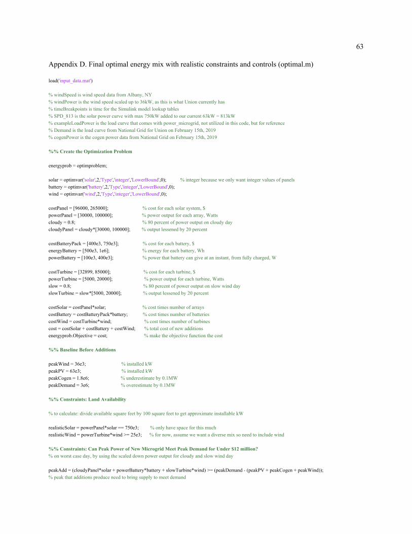
63

Appendix D. Final optimal energy mix with realistic constraints and controls (optimal.m)

load('input_data.mat') % windSpeed is wind speed data from Albany, NY % windPower is the wind speed scaled up to 36kW, as this is what Union currently has % timeBreakpoints is time for the Simulink model lookup tables % SPD_813 is the solar power curve with max 750kW added to our current 63kW = 813kW % exampleLoadPower is the load curve that comes with power_microgrid, not utilized in this code, but for reference % Demand is the load curve from National Grid for Union on February 15th, 2019 % cogenPower is the cogen power data from National Grid on February 15th, 2019 %% Create the Optimization Problem energyprob = optimproblem; solar = optimvar('solar',2,'Type','integer','LowerBound',0); % integer because we only want integer values of panels battery = optimvar('battery',2,'Type','integer','LowerBound',0); wind = optimvar('wind',2,'Type','integer','LowerBound',0); costPanel = [96000, 265000]; % cost for each solar system, $ powerPanel = [30000, 100000]; % power output for each array, Watts cloudy = 0.8; % 80 percent of power output on cloudy day cloudyPanel = cloudy*[30000, 100000]; % output lessened by 20 percent costBatteryPack = [400e3, 750e3]; % cost for each battery, $ energyBattery = [500e3, 1e6]; % energy for each battery, Wh powerBattery = [100e3, 400e3]; % power that battery can give at an instant, from fully charged, W costTurbine = [32899, 85000]; % cost for each turbine, $ powerTurbine = [5000, 20000]; % power output for each turbine, Watts slow = 0.8; % 80 percent of power output on slow wind day slowTurbine = slow*[5000, 20000]; % output lessened by 20 percent costSolar = costPanel*solar; % cost times number of arrays costBattery = costBatteryPack*battery; % cost times number of batteries costWind = costTurbine*wind; % cost times number of turbines cost = costSolar + costBattery + costWind; % total cost of new additions energyprob.Objective = cost; % make the objective function the cost %% Baseline Before Additions peakWind = 36e3; % installed kW peakPV = 63e3; % installed kW peakCogen = 1.8e6; % underestimate by 0.1MW peakDemand = 3e6; % overestimate by 0.1MW %% Constraints: Land Availability % to calculate: divide available square feet by 100 square feet to get approximate installable kW realisticSolar = powerPanel*solar == 750e3; % only have space for this much realisticWind = powerTurbine*wind >= 25e3; % for now, assume we want a diverse mix so need to include wind %% Constraints: Can Peak Power of New Microgrid Meet Peak Demand for Under $12 million? % on worst case day, by using the scaled down power output for cloudy and slow wind day peakAdd = (cloudyPanel*solar + powerBattery*battery + slowTurbine*wind) >= (peakDemand - (peakPV + peakCogen + peakWind)); % peak that additions produce need to bring supply to meet demand

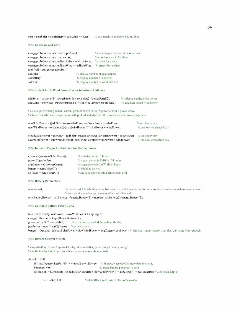
64

cost = costSolar + costBattery + costWind <= 12e6; % cost needs to be below $12 million %% Constrain and solve energyprob.Constraints.conpl = peakAdd; % new supply must meet peak demand energyprob.Constraints.conc = cost; % cost less than $12 million energyprob.Constraints.realisticSolar = realisticSolar; % space for panels energyprob.Constraints.realisticWind = realisticWind; % space for turbines [sol,fval] = solve(energyprob); sol.solar % display number of solar panels sol.battery % display number of batteries sol.wind % display number of wind turbines %% Scale Solar & Wind Power Curves to Include Additions addSolar = sol.solar(1)*powerPanel(1) + sol.solar(2)*powerPanel(2); % calculate added solar power addWind = sol.wind(1)*powerTurbine(1) + sol.wind(2)*powerTurbine(2); % calculate added wind power % ((total power being added / current peak of power curve) * power curve) + power curve % this creates the same shape curve with peak of added power, then sum with what we already have newSolarPower = ((addSolar/(max(solarPower))))*solarPower + solarPower; % on cloudy day newWindPower = ((addWind)/(max(windPower)))*windPower + windPower; % on slow wind speed day cloudySolarPower = (cloudy*((addSolar/(max(solarPower))))*solarPower) + solarPower; % on cloudy day slowWindPower = (slow*((addWind)/(max(windPower)))*windPower) + windPower; % on slow wind speed day %% Initialize Cogen, Geothermal, and Battery Power C = ones(size(newSolarPower)); % initialize vector 1441x1 powerCogen = 2e6; % cogen power is 2MW all 24 hours avgCogen = C*powerCogen; % cogen power is 2MW all 24 hours battery = zeros(size(C)); % initialize battery sellBack = zeros(size(C)); % initialize power sold back to main grid %% Battery Parameters number = 4; % number of 1 MWh lithium ion batteries can be left as one, but for this case it will not be enough to meet demand % so scale this number up by one until it meets demand totalBatteryEnergy = sol.battery(1)*energyBattery(1) + number*sol.battery(2)*energyBattery(2); %% Calculate Battery Power Curve totalGen = cloudySolarPower + slowWindPower + avgCogen; energyDifference = trapz(Demand - totalGen); geo = energyDifference/1441; % extra energy needed throughout the day geoPower = ones(size(C))*(geo); % power curve battery = Demand - (cloudySolarPower + slowWindPower + avgCogen + geoPower); % demand - supply, absorb surplus, discharge if not enough %% Battery Control Scheme % trapz(battery(1:t)) is trapezoidal integration of battery power to get battery energy % multiplied by 1/60 to get from Watt-minutes to Watt-hours (Wh) for t=1:1:1441 if (trapz(battery(1:t))*(1/60)) <= -totalBatteryEnergy % if energy absorbed is more than the rating battery(t) = 0; % make battery power go to zero sellBack(t) = Demand(t) - (cloudySolarPower(t) + slowWindPower(t) + avgCogen(t) + geoPower(t)); % sell back surplus if sellBack(t) > 0 % if sellBack goes positive for some reason

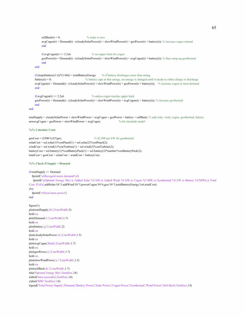
65

sellBack(t) = 0; % make it zero avgCogen(t) = Demand(t) - (cloudySolarPower(t) + slowWindPower(t) + geoPower(t) + battery(t)); % increase cogen instead end if avgCogen(t) >= 2.2e6 % set upper limit for cogen geoPower(t) = Demand(t) - (cloudySolarPower(t) + slowWindPower(t) + avgCogen(t) + battery(t)); % then ramp up geothermal end end if (trapz(battery(1:t))*(1/60)) > totalBatteryEnergy % if battery discharges more than rating battery(t) = 0; % battery caps at that energy, no energy is changed until it needs to either charge or discharge avgCogen(t) = Demand(t) - (cloudySolarPower(t) + slowWindPower(t) + geoPower(t) + battery(t)); % increase cogen to meet demand end if avgCogen(t) >= 2.2e6 % unless cogen reaches upper limit geoPower(t) = Demand(t) - (cloudySolarPower(t) + slowWindPower(t) + avgCogen(t) + battery(t)); % increase geothermal end end totalSupply = cloudySolarPower + slowWindPower + avgCogen + geoPower + battery + sellBack; % add solar, wind, cogen, geothermal, battery newavgCogen = geoPower + slowWindPower + avgCogen; % for simulink model %% Calculate Costs geoCost = (2500/1e3)*geo; % $2,500 per kW for geothermal solarCost = sol.solar(1)*costPanel(1) + sol.solar(2)*costPanel(2); windCost = sol.wind(1)*costTurbine(1) + sol.wind(2)*costTurbine(2); batteryCost = sol.battery(1)*costBatteryPack(1) + sol.battery(2)*number*costBatteryPack(2); totalCost = geoCost + solarCost + windCost + batteryCost; %% Check if Supply > Demand if totalSupply >= Demand fprintf('\nMicrogrid meets demand!\n')

fprintf('\nOptimal Energy Mix:\n Added Solar %f kW,\n Added Wind %f kW,\n Cogen %f MW,\n Geothermal %f kW,\n Battery %f MWh,\n Total Cost: $%f\n',addSolar/10^3,addWind/10^3,powerCogen/10^6,geo/10^3,totalBatteryEnergy/1e6,totalCost) else fprintf('\nNeed more power') end figure(1) plot(totalSupply,'bx','LineWidth',5) hold on plot(Demand,'r','LineWidth',1.7) hold on plot(battery,'g','LineWidth',2) hold on plot(cloudySolarPower,'m','LineWidth',1.5) hold on plot(avgCogen,'black','LineWidth',1.7) hold on plot(geoPower,'c','LineWidth',1.7) hold on plot(slowWindPower,'y-','LineWidth',1.5) hold on plot(sellBack,'b-','LineWidth',1.7) title('Optimal Energy Mix','fontSize',18) xlabel('time (seconds)','fontSize',14) ylabel('MW','fontSize',14) legend('Total Power Supply','Demand','Battery Power','Solar Power','Cogen Power','Geothermal','Wind Power','Sell Back','fontSize',14)

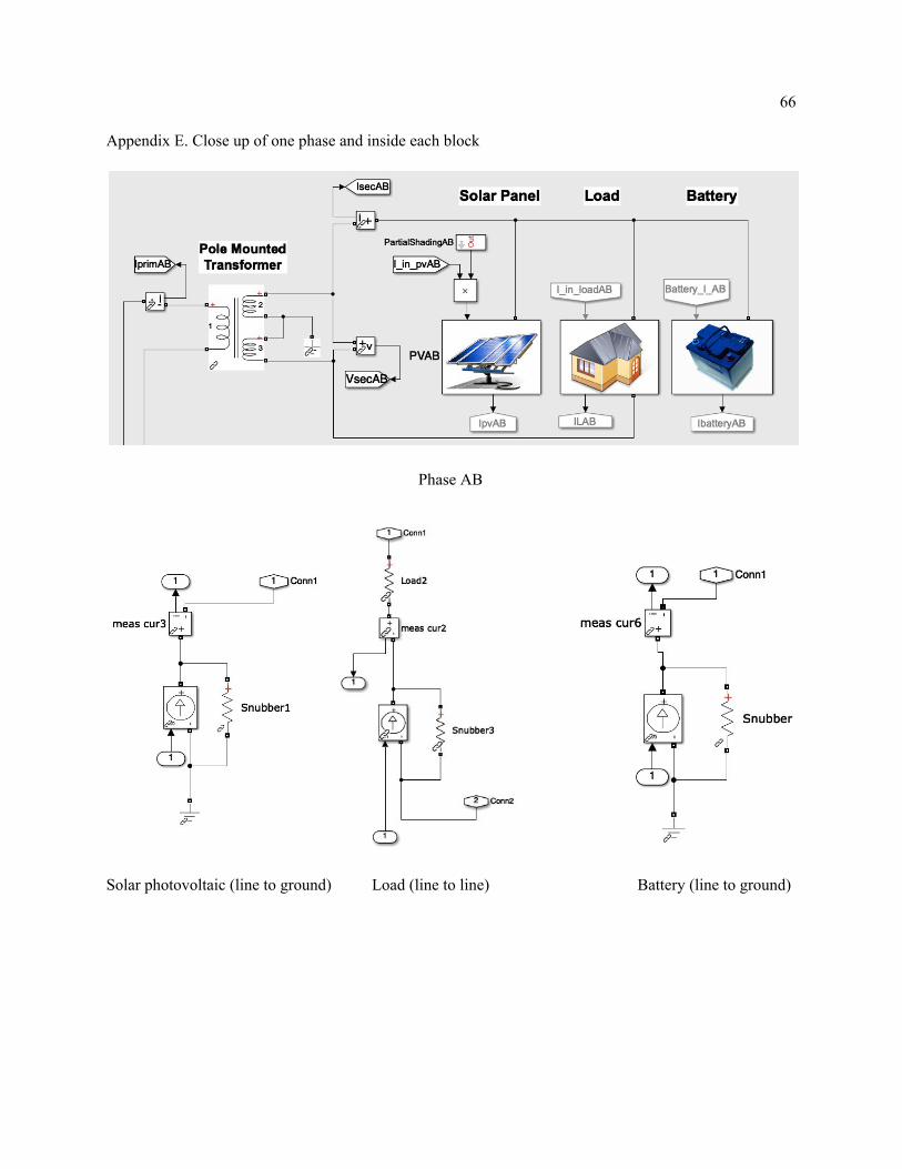
66

Appendix E. Close up of one phase and inside each block

Phase AB

Solar photovoltaic (line to ground) Load (line to line) Battery (line to ground)