University of North DakotaUND Scholarly Commons

Theses and Dissertations Theses, Dissertations, and Senior Projects

January 2013

Optimization Of The GARCH Model ParametersUsing A Genetic AlgorithmJonathon Patrick Cummings

Follow this and additional works at: https://commons.und.edu/theses

This Thesis is brought to you for free and open access by the Theses, Dissertations, and Senior Projects at UND Scholarly Commons. It has beenaccepted for inclusion in Theses and Dissertations by an authorized administrator of UND Scholarly Commons. For more information, please contactzeineb.yousif@library.und.edu.

Recommended CitationCummings, Jonathon Patrick, "Optimization Of The GARCH Model Parameters Using A Genetic Algorithm" (2013). Theses andDissertations. 1411.https://commons.und.edu/theses/1411

OPTIMIZATION OF THE GARCH MODEL PARAMETERS USING A

GENETIC ALGORITHM

by

Jonathon Patrick Cummings

A Thesis

Submitted to the Graduate

Faculty of the University of

North Dakota in partial

fulfillment of the

requirements

for the degree of

Master of

Science

Grand Forks, North Dakota

August

2013

iii

PERMISSION

Title: OPTIMIZATION OF THE GARCH MODEL PARAMETERS USING A GENETIC ALGORITHM

Department: Applied Economics

Degree: Master of Science in Applied Economics

In presenting this thesis in partial fulfillment of the requirements for a graduate degree

from the University of North Dakota, I agree that the library of this University shall

make it freely available for inspection. I further agree that permission for extensive

copying for scholarly purposes may be granted by the professor who supervised my

thesis work or, in his absence, by the Chairperson of the department or the dean of the

Graduate School. It is understood that any copying or publication or other use of this

thesis or part thereof for financial gain shall not be allowed without my written

permission. It is also understood that due recognition shall be given to me and to the

University of North Dakota in any scholarly use which may be made of any material in

my thesis.

Jonathon P. Cummings

August 2013

iv

TABLE OF CONTENTS

LIST OF FIGURES………………….…………………………………………………………………………………..….…….…...…...v

LIST OF TABLES…………………….……………………………………………….……….………………………………...…….…….vi

ACKNOWLEDGMENTS………………………………………………………………..………..………………...……....…….….vii

ABSTRACT…………………………………………………………………………..…………..……………………………..…...………..viii

CHAPTER

I. INTRODUCTION……………...……..…..…………………...…………………………………………..….….…..….1

II. LITERATURE REVIEW………..….………….…………………………………..…………………....…..……4

III. METHODOLOGY…………….……………………………………………….…...………...……………..……....7

IV. RESULTS……………..…………...…...……….….………………………………………………..….………..….…..12

V. FUTURE RESEARCH………….………………….………………………………….……..…...……..…….16

VI. SUMMARY…………………….…………………………………………………..…………...……….….………18

REFERENCES………………….……………………………………………..…………………………………....……….….….……19

v

LIST OF FIGURES

Figure _Page

D-GARCH vs. GARCH(1,1), difference in log volatilities……………..………………..……….….………….12

D-GARCH vs. GARCH(1,1) Log Volatilities………………………………………………………...…..…..…………...13

20-Period S&P 500 Percentage Change…………………………………………………………..…..………….…......…14

S&P 500 Index Close……………………………………………………………….……………….……………….……..…….….…..14

vi

LIST OF TABLES

Table _Page

Interpolated Dickey-Fuller – raw data………………………………………………………………………....…….………7

Interpolated Dickey-Fuller – daily percentage change…………………………………………….……….…….7

One-period regression on lagged percentage change………………………....................................….………….8

One-period regression on lagged squared residuals………..………………………………………..….…………..8

GARCH(1,1) regression on one-period lagged residuals……………. ………..………...……………….9

vii

ACKNO WLEDGMENTS

I wish to thank my Professors at the University of North Dakota for their

knowledgeable instruction and passion for the topic of Applied Economics. I further want to

thank my parents for their unending support and my three wonderful children for their patience

and understanding in pursuit of this degree.

viii

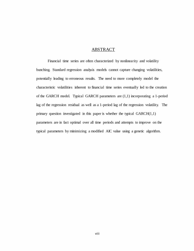
ABS TRACT

Financial time series are often characterized by nonlinearity and volatility

bunching. Standard regression analysis models cannot capture changing volatilities,

potentially leading to erroneous results. The need to more completely model the

characteristic volatilities inherent to financial time series eventually led to the creation

of the GARCH model. Typical GARCH parameters are (1,1) incorporating a 1-period

lag of the regression residual as well as a 1-period lag of the regression volatility. The

primary question investigated in this paper is whether the typical GARCH(1,1)

parameters are in fact optimal over all time periods and attempts to improve on the

typical parameters by minimizing a modified AIC value using a genetic algorithm.

1

CHAPTER I

INTRODUCTION

The desire to understand the nature and characteristics of time series data has

led to the development of a variety of models. Models that focus on the character of

the data, or some derivative of the data, range from the basic moving average (MA) to

the more complicated autoregressive moving average (ARMA). These models attempt

to understand the nature of the data itself versus some other characteristic of the data,

such as volatility. Other models, such as the autoregressive conditional

heteroskedasticity (ARCH) created by Robert Engle, do indeed focus on the

underlying volatility b y examining the lag structure of the squared residuals.1

However, ARCH remained unsatisfactory because it neglected to incorporate any

additional regression term that allowed for the persistence of economic shocks.

Finally in 1986, Tim Peter Bollerslev presented the GARCH model for

Generalized Autoregressive Conditional Heteroskedasticity. 2 GARCH represented an

improvement over the ARCH model in that where ARCH was only conditioned on

lagged square residuals, GARCH added the additional component of lagged conditioned

variances. Additionally, the GARCH model allowed for corrections related to time

1 Aut or e g r e s s i v e Conditional Het e ro s c e d a s t i ci t y with Es timates of the Variance of United

Kingdo m Inflation,” Robert F. Engle, Econometrica , Vol. 50, No. 4 (Jul., 1982), pp. 987-1007.

2 "Genera l i zed Autoregress i ve Condi ti ona l Heteros keda s ti city,” Boll ers lev, Ti m, Journal of

Econometrics 31 (3): 307–327, 1986.

2

series that exhibited thick tail distributions and volatility clustering, both of which are

common, especially in nonlinear financial time series. For example, the following

describes the ARCH process in which the current period’s volatility is conditio ned on

the regressive sum of the lagged residuals up to period t-q:

Conversely, the GARCH model is represented as follows:

Note the additional conditioning terms representing lagged period volatilities up to

period t-p. These additional conditioning factors allow for the periodic economic

shocks to reverberate longer in the data than simply one period.

One of the concerns of the GARCH model, or any time series model that uses

lagged terms, is the value for q and p. In other words, how many lags should be

included in the model to best reflect the underlying character of the data? Typically

this is a choice made by the modeler and will depend on the model’s forecasting

abilit y as a GARCH(1,1) process, or perhaps a GARCH(4,4) if working with

quarterly data. Once the choice is made, it is then applied to the entire data series

without concern for potential inherent changes in the data over time.

Therefore, the purpose of this paper is to present a possible solution to the

question of the optimal number of lagged periods for (p,q) in the GARCH model.

Through the use of an optimization tool called a Genetic Algorithm, or GA, it will be

shown that the GARCH(1,1) model is not always the best solution when searching for

3

the optimal values for (p,q). Furthermore, it will be shown that the optimal values for

(p,q) in fact change over time, reflecting the dynamic, effervescent nature of financial

time series. The resulting model is hereafter termed as the D-GARCH with the “D”

representing “dynamic.”

4

CHAPTER II

LITERATURE REVIEW

A great deal of literature has examined the GARCH model and its parameters as

well as methods for optimizing those parameters, includ ing the use of genetic algorithms

and neural networks. These techniq ues are referred to as “fuzzy,” or artificial intelligence

methods for finding optimal solutions to problems which are typically difficult to solve

using classical methods.

The literature is divided into essentially two categories: the need for better

modeling of nonlinear systems such as the financial markets and possible tools and

methods with which the models might be improved. The literature devoted to these

questions is plentiful. A few noteworthy and relevant examples are given in this section.

Regarding the very concept of volatility itself, Nwogugu noted that volatility “can

be modeled as the sum of all preferences of market participants over time,” indicating that

volatility in market prices is derived from investor utility. As such, models such as the

traditional GARCH are “structurally deficient and static.”3 Nonlinear, adaptive, fuzzy

modeling was needed to adequately capture the dynamics of financial time series. Doing

so required a search for optimal solutions in multi-dimensional, nonlinear solution spaces.

Adanu noted that in any search for optimization, it is important to keep in mind that a

3 Nwogugu, Michael. 2006. "Volatility, ris k modeling and utility." Applied Mathematics &

Computation 182, no. 2: 1749-1754.

5

global optimum must be sought and to take care not to use methods that may be drawn to

only local optima. In other words, the researcher should utilize methods that are not

contingent on a defined starting point, such as Newton’s algorithm, the simplex method,

or the conjugate gradient methods.4 Specifically addressing the GARCH model, Altay-

Salih, et al, supported the notion that fuzzy programming, i.e. nonlinear programming

without artificial restraints imposed by the modeler, produced better results than the

traditional GARCH model, especially when bivariate and trivariate cases are considered.5

Given the need for fuzzy programming to analyze the dynamics of nonlinear time

series, other researchers applied techniques such as genetic algorithms. Nair, et al,

suggested the use of a genetic algorithm to optimize a decision tree based on 28 popular

technical indicators. It was noted that a genetic algorithm is a “parallel search algorithm”

which in this case was used to minimize trend prediction error.6 Li, et al, employed

genetic algorithm methods to study the scaling properties of wavelet-based indicators for

the Dow Jones Industrial Average, allowing for the study of price data at multip le time

scales.7 Havandi, et al, explore integrating genetic algorithms and neural networks for

stock price prediction in the IT and Airline sectors with the goal of capitalizing on the

4 Adanu, Kwami. 2006. “Optimizing the GARCH Model – An Application of Two Global and

Two Local Search Methods .” Computational Economics , no.28: 277-290.

5 Altay-Salih, As lihan, Mus tafa C. Pinar, and Sven Leyffer. 2003. "Cons trained Nonlinear

Programming for Volatility Es timation with GARCH Models ." SIAM Review 45, no. 3: 485-503.

6 Nair, Binoy B., V. P. Mohandas , and N. R. Sakthivel. 2010. "A Genetic Algorithm Optimized

Decis ion Tree- SVM bas ed Stock Market Trend Prediction Sys tem." International Journal On Computer

Science & Engineering 2981-2988.

7 Jin, Li, Shi Zhu, and Li Xiaoli. 2006. "Genetic programming with wavelet-bas ed indicators for

financial forecas ting." Transactions Of The Institute Of Measurement & Control 28, no. 3: 285-297.

s eries volatility." Journal Of Intelligent & Fuzzy Systems 23, no. 1: 27-38.

6

strengths of each method.8

Other researchers turned their attention to the GARCH model specifically. Roh

compared the performance of various time series forecasting models such as GARCH,

EGARCH and Exponentially Weighted Moving Average when optimized using adaptive

neural networks. Roh’s focus was not on stock price movement, but rather on the

direction and deviation of the stock’s volatility. 9 Hung also examined the idea of

optimizing the GARCH model as well as more recent innovations of the model

(EGARCH, GJR-GARCH, and Fuzzy GARCH). Hung’s approach was to use a “particle

swarm optimization” (PSO) model which imitates the movement of a swarm of gnats or a

flock of birds. The PSO method, like the genetic algorithm, evaluates multip le possible

solutions in the solution space to quickly arrive at a global maximum (or minimum

depending on the objective).10 Finally, Luna and Ballini studied the use of an adaptive

fuzzy interface system (AdaFIS) to directly evaluate volatility and value-at-risk (VAR) in

an effort to improve on traditio nal measures like GARCH.11

The literature summarized here is a merely a smattering of the research done on

the application of fuzzy programming to nonlinear models. The remainder of this paper

will summarize another possible method with which to optimize the GARCH model.

8 Hadavandi, Es maeil, Has s an Shavandi, and Aras h Ghanbari. 2010. "Integration of genetic fuzzy

s ys tems and artificial neural networks for s tock price forecas ting." Knowledge-Based Systems 23, no. 8:

800-808.

9 Hyup Roh, Tae. 2007. "Forecas ting the volatility of s tock price index." Expert Systems With

Applications 33, no. 4: 916-922.

10 Hung, Jui-Chung. 2011. "Adaptive Fuzzy-GARCH model applied to forecas ting the volatility of

s tock markets us ing particle s warm optimization." Information Sciences 181, no. 20: 4673-4683.

11 Luna, Ivette, and Ros angela Ballini. 2012. "Adaptive fuzzy s ys tem to forecas t financial time

7

CHAPTER III

METHODOLOGY

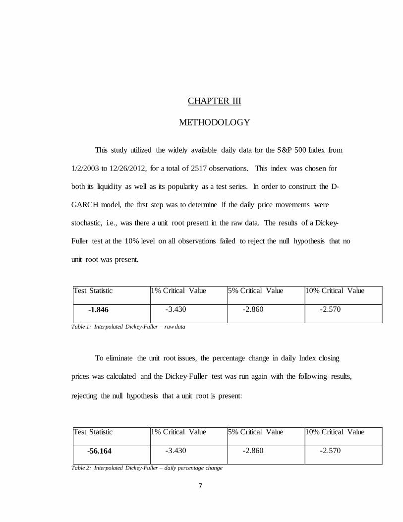
This study utilized the widely available daily data for the S&P 500 Index from

1/2/2003 to 12/26/2012, for a total of 2517 observations. This index was chosen for

both its liquidity as well as its popularity as a test series. In order to construct the D-

GARCH model, the first step was to determine if the daily price movements were

stochastic, i.e., was there a unit root present in the raw data. The results of a Dickey-

Fuller test at the 10% level on all observations failed to reject the null hypothesis that no

unit root was present.

Test Statistic 1% Critical Value 5% Critical Value 10% Critical Value

-1.846 -3.430 -2.860 -2.570

Table 1: Interpolated Dickey-Fuller – raw data

To eliminate the unit root issues, the percentage change in daily Index closing

prices was calculated and the Dickey-Fuller test was run again with the following results,

rejecting the null hypothesis that a unit root is present:

Test Statistic 1% Critical Value 5% Critical Value 10% Critical Value

-56.164 -3.430 -2.860 -2.570

Table 2: Interpolated Dickey-Fuller – daily percentage change

8

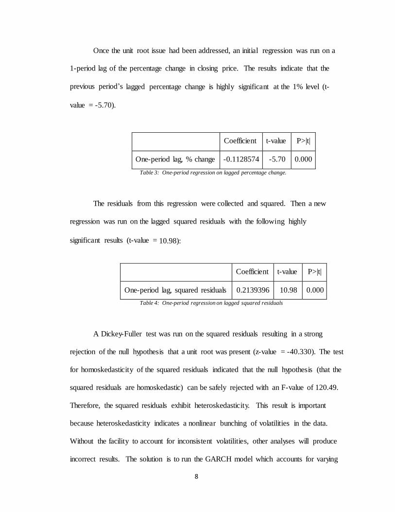
Once the unit root issue had been addressed, an initial regression was run on a

1-period lag of the percentage change in closing price. The results indicate that the

previous period’s lagged percentage change is highly significant at the 1% level (t-

value = -5.70).

Coefficient

t-value

P>|t|

One-period lag, % change

-0.1128574

-5.70

0.000

Table 3: One-period regression on lagged percentage change.

The residuals from this regression were collected and squared. Then a new

regression was run on the lagged squared residuals with the following highly

significant results (t-value = 10.98):

Coefficient

t-value

P>|t|

One-period lag, squared residuals

0.2139396

10.98

0.000

Table 4: One-period regression on lagged squared residuals

A Dickey-Fuller test was run on the squared residuals resulting in a strong

rejection of the null hypothesis that a unit root was present (z-value = -40.330). The test

for homoskedasticity of the squared residuals indicated that the null hypothesis (that the

squared residuals are homoskedastic) can be safely rejected with an F-value of 120.49.

Therefore, the squared residuals exhibit heteroskedasticity. This result is important

because heteroskedasticity indicates a nonlinear bunching of volatilities in the data.

Without the facility to account for inconsistent volatilities, other analyses will produce

incorrect results. The solution is to run the GARCH model which accounts for varying

9

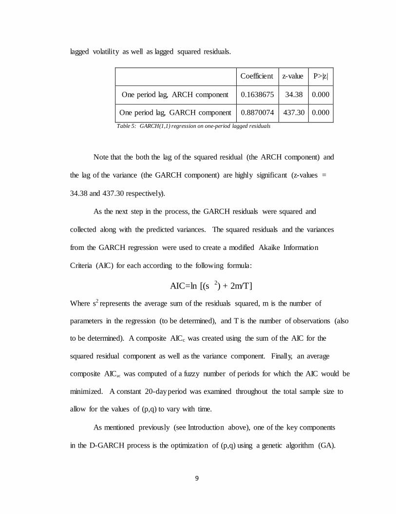
lagged volatility as well as lagged squared residuals.

Coefficient

z-value

P>|z|

One period lag, ARCH component

0.1638675

34.38

0.000

One period lag, GARCH component

0.8870074

437.30

0.000

Table 5: GARCH(1,1) regression on one-period lagged residuals

Note that the both the lag of the squared residual (the ARCH component) and

the lag of the variance (the GARCH component) are highly significant (z-values =

34.38 and 437.30 respectively).

As the next step in the process, the GARCH residuals were squared and

collected along with the predicted variances. The squared residuals and the variances

from the GARCH regression were used to create a modified Akaike Information

Criteria (AIC) for each according to the following formula:

AIC=ln [(s 2) + 2m/T]

Where s2 represents the average sum of the residuals squared, m is the number of

parameters in the regression (to be determined), and T is the number of observations (also

to be determined). A composite AICc was created using the sum of the AIC for the

squared residual component as well as the variance component. Finally, an average

composite AICac was computed of a fuzzy number of periods for which the AIC would be

minimized. A constant 20-day period was examined throughout the total sample size to

allow for the values of (p,q) to vary with time.

As mentioned previously (see Introduction above), one of the key components

in the D-GARCH process is the optimization of (p,q) using a genetic algorithm (GA).

10

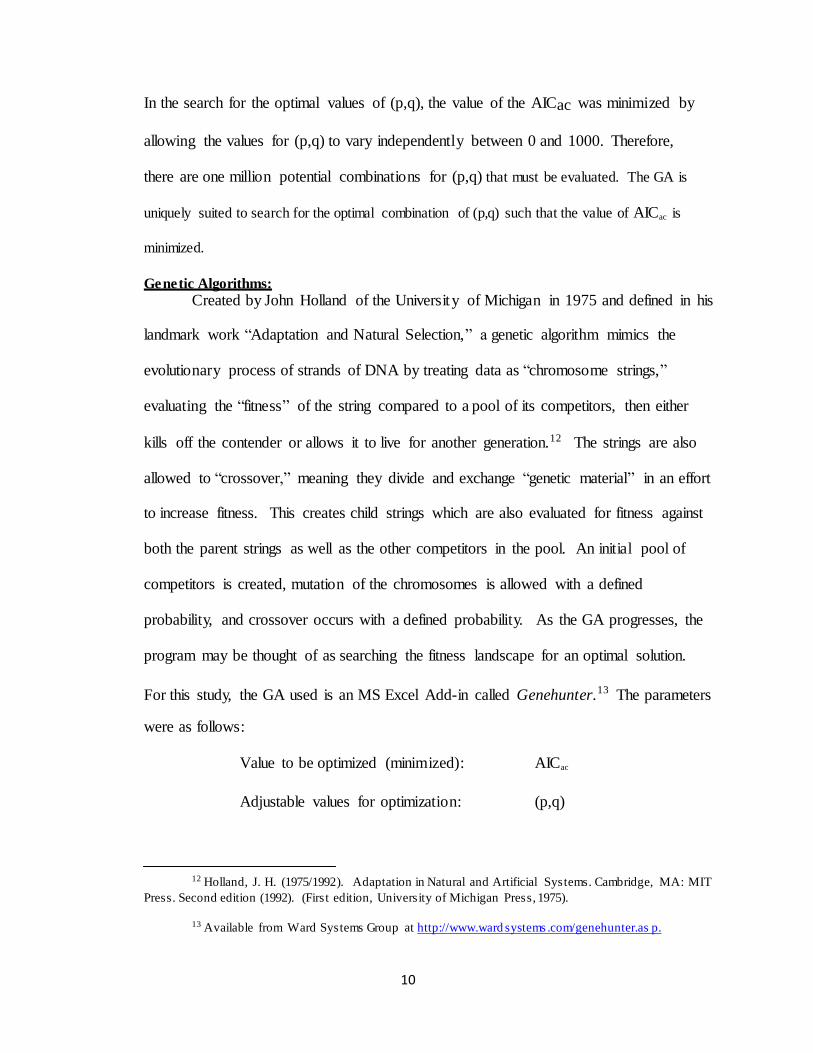
In the search for the optimal values of (p,q), the value of the AICac was minimized by

allowing the values for (p,q) to vary independently between 0 and 1000. Therefore,

there are one million potential combinatio ns for (p,q) that must be evaluated. The GA is

uniquely suited to search for the optimal combination of (p,q) such that the value of AICac is

minimized.

Ge ne tic Algorithms:

Created by John Holland of the Universit y of Michigan in 1975 and defined in his

landmark work “Adaptation and Natural Selection,” a genetic algorithm mimics the

evolutio nary process of strands of DNA by treating data as “chromosome strings,”

evaluating the “fitness” of the string compared to a pool of its competitors, then either

kills off the contender or allows it to live for another generation.12 The strings are also

allowed to “crossover,” meaning they divide and exchange “genetic material” in an effort

to increase fitness. This creates child strings which are also evaluated for fitness against

both the parent strings as well as the other competitors in the pool. An initial pool of

competitors is created, mutation of the chromosomes is allowed with a defined

probability, and crossover occurs with a defined probability. As the GA progresses, the

program may be thought of as searching the fitness landscape for an optimal solution.

For this study, the GA used is an MS Excel Add-in called Genehunter.13 The parameters

were as follows:

Value to be optimized (minimized): AICac

Adjustable values for optimization: (p,q)

12 Holland, J. H. (1975/1992). Adaptation in Natural and Artificial Sys tems . Cambridge, MA: MIT

Press . Second edition (1992). (Firs t edition, Univers ity of Michigan Press , 1975).

13 Available from Ward Sys tems Group at http:/ /www.ward s ystems .com/genehunter.as p.

11

Range of possible values for (p,q): 0-1000

Initial population: 100

Probability of crossover: 90%

Probability of mutation: 1%

Evolution cutoff: 100 generations

The GA was run over non-overlapping 20-day periods. The initial period was (t,

t-20), then (t-21, t-40), etc… througho ut the 2517 observation sample. In total, 76 20-

period blocks were evaluated by the GA. The optimal (minimized) AICac, p, and q were

recorded as well as the AICac with (p,q) = (1,1), or a basic GARCH(1,1) model.

Optimized pairs of (p,q) which minimize AICac, and thus define the optimal GARCH

parameters, could range from (0,0), or no lag terms, to (1000,1000).

Once the optimized pairs were determined by the GA, the volatility was calculated

according to the GARCH equation in Chapter 1 above. For comparison purposes, the

volatility implied by the GARCH(1,1) model was also calculated. The logs of both were

calculated and summarized for further analysis.

12

01

/01

/07

04

/01

/07

07

/01

/07

10

/01

/07

01

/01

/08

04

/01

/08

07

/01

/08

10

/01

/08

01

/01

/09

04

/01

/09

07

/01

/09

10

/01

/09

01

/01

/10

04

/01

/10

07

/01

/10

10

/01

/10

01

/01

/11

04

/01

/11

07

/01

/11

10

/01

/11

01

/01

/12

04

/01

/12

07

/01

/12

CHAPTER IV

RESULTS

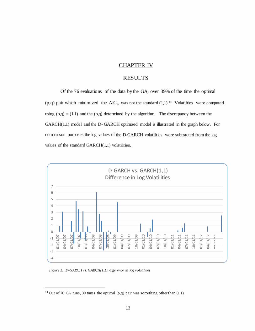
Of the 76 evaluations of the data by the GA, over 39% of the time the optimal

(p,q) pair which minimized the AICac was not the standard (1,1).14 Volatilities were computed

using (p,q) = (1,1) and the (p,q) determined by the algorithm. The discrepancy between the

GARCH(1,1) model and the D- GARCH optimized model is illustrated in the graph below. For

comparison purposes the log values of the D-GARCH volatilities were subtracted from the log

values of the standard GARCH(1,1) volatilities.

D-GARCH vs. GARCH(1,1)

Difference in Log Volatilities

7

6

5

4

3

2

1

0

-1

-2

-3

-4

Figure 1: D-GARCH vs. GARCH(1,1), difference in log volatilities

14 Out of 76 GA runs , 30 times the optimal (p,q) pair was s omething other than (1,1).

13

01

/01

/07

04

/01

/07

07

/01

/07

10

/01

/07

01

/01

/08

04

/01

/08

07

/01

/08

10

/01

/08

01

/01

/09

04

/01

/09

07

/01

/09

10

/01

/09

01

/01

/10

04

/01

/10

07

/01

/10

10

/01

/10

01

/01

/11

04

/01

/11

07

/01

/11

10

/01

/11

01

/01

/12

04

/01

/12

07

/01

/12

GARCH(1,1) VOLATILITY VS. D-GARCH VOLATILITY

12

10

8

6

4

2

0

-2

D-GARCH GARCH(1,1)

Figure 2: D-GARCH vs. GARCH(1,1) Log Volatilities

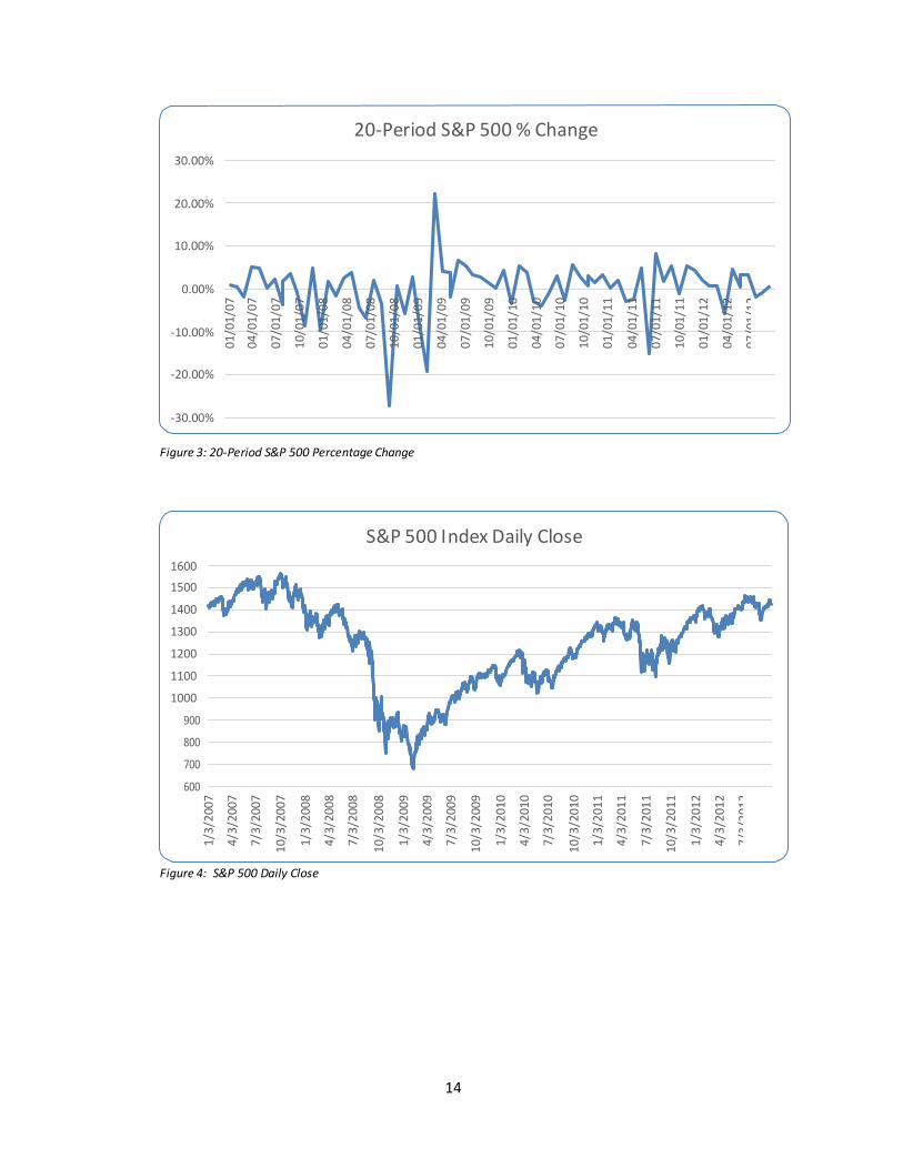
Note in the graph above that the D-GARCH volatilities tend to emphasize the

“frothiness” of the market more than the traditional GARCH(1,1) model, producing

higher peaks. This is especially evident during the turbulent downturn and subsequent

recovery of the S&P 500 Index as illustrated in the following two graphs:

14

1/3

/200

7

4/3

/200

7

7/3

/200

7 1

0/3

/20

07

1/3

/200

8

4/3

/20

08

7/3

/200

8 1

0/3

/20

08

1/3

/200

9

4/3

/200

9

7/3

/200

9 1

0/3

/200

9

1/3

/201

0

4/3

/201

0

7/3

/201

0 1

0/3

/20

10

1/3

/201

1

4/3

/201

1

7/3

/201

1 1

0/3

/20

11

1/3

/201

2

4/3

/201

2

7/3

/201

2

01

/01

/07

04

/01

/07

07

/01

/07

10

/01

/07

01

/01

/08

04

/01

/08

07

/01

/08

10

/01

/08

01

/01

/09

04

/01

/09

07

/01

/09

10

/01

/09

01

/01

/10

04

/01

/10

07

/01

/10

10

/01

/10

01

/01

/11

04

/01

/11

07

/01

/11

10

/01

/11

01

/01

/12

04

/01

/12

07

/01

/12

20-Period S&P 500 % Change

30.00%

20.00%

10.00%

0.00%

-10.00%

-20.00%

-30.00%

Figure 3: 20-Period S&P 500 Percentage Change

1600

1500

1400

1300

1200

1100

1000

900

800

700

600

S&P 500 I ndex Daily Close

Figure 4: S&P 500 Daily Close

15

The determination of which combination of (p,q) was optimal was based strictly

in minimizing the modified AIC as described above. In doing so, this study was able to

focus strictly on the information that could be gleaned from the data series. Certainly

other variables could be introduced (interest rates, quarterly GDP, etc…), but the

univariate GARCH was used to isolate the optimal (p,q) found through the GA. The

results from using the GA to determine the optimal (p,q) ranged from (1,1) to

(1000,1000). The periods during which the algorithm found the greater values for (p,q)

corresponded to periods of higher volatility, especially during the recessionary period

from mid-2008 to mid-2009 (see graphs above).

Additionally, it should be noted that other criteria for discriminating

among potential (p,q) combinations could be implemented. Other information criteria

such as the Bayesian Information Criteria (BIC) could be tested. Another possibility is

to generate a test to determine which (p,q) combination minimizes the difference

between the calculated volatilities and the historical standard deviation for the same test

data. These other possibilities were not addressed in this study.

16

CHAPTER V

FUTURE RESEARCH

The optimization of the GARCH parameters through the use of the GA as

described above may have direct application to investment strategy, particularly to option

trading. For example, the heralded Black-Scholes option valuation model incorporates a

volatility factor according to the following formula for the value of a European call

option15:

Value of call option: C = SN(d1) – Ke-rt

N(d2)

Where: d1 = [ln(S/K) + (r + v/2)T] / (v*T)1/2

d2 = d1 – (v*T)1/2

S = current stock or index price

K = strike price

N = cumulative standard normal distribution

r = risk-free rate of return

v = volatility

T = time until option expiration

All of the factors of the Black-Scholes option valuation model are explicitly

known at any period in time except for the volatility (v). The computed values for

15 Black, Fischer; Myron Scholes (1973). "The Pricing of Options and Corporate Liabilities ".

Journal of Political Economy 81 (3): 637–654.

17

ln(h(t)) may be easily used to calculate the theoretical option values and compared with

the actual option values to identify discrepancies, and therefore potential trading

opportunities. One of the inherent issues with the Black-Scholes model is the assumption

of constant volatility over a given period of time (for example annualized). Due to the

dynamic nature of the D-GARCH process, it may prove to better calculate true volatility

and thus more accurately reflect the current theoretical option value.

This paper addressed the D-GARCH process in discrete 20-day blocks of daily

closing data for the S&P 500 Index. Other additional research possibilities include

replicating this study using weekly, quarterly, and annual data over other data samples

and other financial markets, as well as other criteria for determining optimality of the

(p,q) combination.

18

CHAPTER VI

SUMMARY

The D-GARCH process utilizes a modified Akaike Information Criteria (AIC)

optimized using a genetic algorithm to identify the optimal parameters for the GARCH

model of time series volatility. The D-GARCH model produced a more optimal solution

in 39% of the cases sampled while agreeing with the traditional GARCH(1,1) model in

61% of the cases. In particular, when the market under study (S&P 500 Index) becomes

more “frothy,” the D-GARCH better highlights the extreme volatility than the

GARCH(1,1) model. It remains to be seen if the application of the volatilities calculated

by the D-GARCH process can better calculate theoretical options prices.

19

REFERENCES

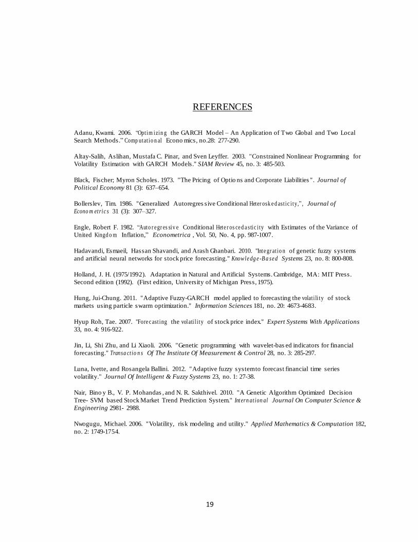
Adanu, Kwami. 2006. “Op t i m i zi n g the GARCH Model – An Application of T wo Global and Two Local

Search Methods .” Co mp u t at i o n al Econo mics , no.28: 277-290.

Altay-Salih, As lihan, Mus tafa C. Pinar, and Sven Leyffer. 2003. "Cons trained Nonlinear Programming for

Volatility Es timation with GARCH Models ." SIAM Review 45, no. 3: 485-503.

Black, Fis cher; Myron Scholes . 1973. "The Pricing of Optio ns and Corporate Liabilities ". Journal of

Political Economy 81 (3): 637–654.

Bollers lev, Tim. 1986. "Generalized Autoregres s ive Conditional Het er o sk e d as t i c i t y ,” , Journal of

Econo m et r i c s 31 (3): 307–327.

Engle, Robert F. 1982. “Aut o r e g r es si v e Conditional Hete r o s ce d a s ti c i t y with Es timates of the Variance of

United King d o m Inflation,” Econometrica , Vol. 50, No. 4, pp. 987-1007.

Hadavandi, Es maeil, Has s an Shavandi, and Aras h Ghanbari. 2010. "Inte g r at i o n of genetic fuzzy s ys tems

and artificial neural networks for s tock price forecas ting." Kno w le dg e -B a s e d Systems 23, no. 8: 800-808.

Holland, J. H. (1975/1992). Adaptation in Natural and Artificial Sys tems . Cambridge, MA: MIT Press .

Second edition (1992). (Firs t edition, Univers ity of Michigan Press , 1975).

Hung, Jui-Chung. 2011. "Adaptive Fuzzy-GARCH model applied to forecas ting the volat i li t y of s tock

markets us ing particle s warm optimization." Information Sciences 181, no. 20: 4673-4683.

Hyup Roh, Tae. 2007. "Fore c as t i n g the vol ati l i t y of s tock price index." Expert Systems With Applications

33, no. 4: 916-922.

Jin, Li, Shi Zhu, and Li Xiaoli. 2006. "Genetic programming with wavelet-bas ed indicators for financial

forecas ting." Tran s a ct io n s Of The Institute Of Measurement & Control 28, no. 3: 285-297.

Luna, Ivette, and Ros angela Ballini. 2012. "Adaptive fuzzy s ys tem to forecas t financial time s eries

volatility." Journal Of Intelligent & Fuzzy Systems 23, no. 1: 27-38.

Nair, Bino y B., V. P. Mohandas , and N. R. Sakthivel. 2010. "A Genetic Algorithm Optimized Decis ion

Tree- SVM bas ed Stock Market Trend Prediction System." Int er n a t i on a l Journal On Computer Science &

Engineering 2981- 2988.

Nwogugu, Michael. 2006. "Volatility, ris k modeling and utility." Applied Mathematics & Computation 182,

no. 2: 1749-1754.