Optimization Of Ocean Thermal Energy Conversion Power Plants

University of Central Florida University of Central Florida

STARS STARS

Electronic Theses and Dissertations, 2004-2019

2012

Optimization Of Ocean Thermal Energy Conversion Power Plants Optimization Of Ocean Thermal Energy Conversion Power Plants

Steven Emanoel Rizea University of Central Florida

Part of the Mechanical Engineering Commons

Find similar works at: https://stars.library.ucf.edu/etd

University of Central Florida Libraries http://library.ucf.edu

This Masters Thesis (Open Access) is brought to you for free and open access by STARS. It has been accepted for

inclusion in Electronic Theses and Dissertations, 2004-2019 by an authorized administrator of STARS. For more

information, please contact [email protected].

STARS Citation STARS Citation Rizea, Steven Emanoel, "Optimization Of Ocean Thermal Energy Conversion Power Plants" (2012). Electronic Theses and Dissertations, 2004-2019. 2368. https://stars.library.ucf.edu/etd/2368

https://stars.library.ucf.edu/



https://stars.library.ucf.edu/etd

http://network.bepress.com/hgg/discipline/293?utm_source=stars.library.ucf.edu%2Fetd%2F2368&utm_medium=PDF&utm_campaign=PDFCoverPages

https://stars.library.ucf.edu/etd

http://library.ucf.edu/

mailto:[email protected]

https://stars.library.ucf.edu/etd/2368?utm_source=stars.library.ucf.edu%2Fetd%2F2368&utm_medium=PDF&utm_campaign=PDFCoverPages



OPTIMIZATION OF OCEAN THERMAL ENERGY CONVERSION POWER PLANTS

by

STEVEN EMANOEL RIZEA

B.S. University of Florida, 2006

A thesis submitted in partial fulfillment of the requirements

for the degree of Master of Science in Mechanical Engineering

in the Department of Mechanical, Materials, and Aerospace Engineering

in the College of Engineering and Computer Science

at the University of Central Florida

Orlando, Florida

Summer Term

2012

ii

© 2012 Steven Emanoel Rizea

iii

ABSTRACT

A proprietary Ocean Thermal Energy Conversion (OTEC) modeling tool, the Makai

OTEC Thermodynamic and Economic Model (MOTEM), is leveraged to evaluate the accuracy

of finite-time thermodynamic OTEC optimization methods. MOTEM is a full OTEC system

simulator capable of evaluating the effects of variation in heat exchanger operating temperatures

and seawater flow rates. The evaluation is based on a comparison of the net power output of an

OTEC plant with a fixed configuration. Select optimization methods from the literature are

shown to produce between 93% and 99% of the maximum possible amount of power, depending

on the selection of heat exchanger performance curves. OTEC optimization is found to be

dependent on the performance characteristics of the evaporator and condenser used in the plant.

Optimization algorithms in the literature do not take heat exchanger performance variation into

account, which causes a discrepancy between their predictions and those calculated with

MOTEM.

A new characteristic metric of OTEC optimization, the ratio of evaporator and condenser

overall heat transfer coefficients, is found. The heat transfer ratio is constant for all plant

configurations in which the seawater flow rate is optimized for any particular evaporator and

condenser operating temperatures. The existence of this ratio implies that a solution for the ideal

heat exchanger operating temperatures could be computed based on the ratio of heat exchanger

performance curves, and additional research is recommended.

iv

Dedicated to my lovely wife Leighanna, without whose support this would not have been

possible.

v

ACKNOWLEDGMENTS

The completion of this paper required the assistance of friends, family, and colleagues. I

would like to thank select individuals who made a particular contribution. Firstly, I must

acknowledge the assistance of my adviser, Professor Marcel Ilie. His guidance, patience, and

focus on helping students excel were invaluable in the completion of my research.

Secondly, I would like to extend special thanks to Makai Ocean Engineering for granting

access to their Makai OTEC Thermodynamic and Economic Model, with which most of the

calculations for this project were performed. In addition, their long-term support has made my

foray into graduate school possible.

Last, but certainly not least, I would like to thank my friends and family for their support.

My wife, in particular, has exhibited a boundless capacity for sacrificing weekends, quiet

evenings at home, and no small number of special events in the name of my education.

vi

TABLE OF CONTENTS

LIST OF FIGURES ........................................................................................................................ x

LIST OF TABLES ......................................................................................................................... xi

LIST OF SYMBOLS .................................................................................................................... xii

1. INTRODUCTION .................................................................................................................. 1

1.1. Basic OTEC Heat Engine ................................................................................................. 1

1.2. Design Challenges ............................................................................................................ 3

1.2.1. Heat Engine Efficiency ............................................................................................. 4

1.2.2. Seawater Flow Rate .................................................................................................. 8

1.2.3. Impact on OTEC Design ........................................................................................... 8

2. LITERATURE REVIEW ..................................................................................................... 10

2.1. Isothermal Heat Reservoirs with a Carnot Engine ......................................................... 11

2.1.1. Limiting Assumptions ............................................................................................. 12

2.2. Heat Reservoirs with Varying Heat Capacity Rate and a Rankine Engine .................... 13

2.2.1. Limiting Assumptions ............................................................................................. 14

3. MODELING REAL OTEC SYSTEMS ............................................................................... 16

3.1. Theoretical Magnification of the Effects of Variation in Optimization Parameters ...... 16

3.2. Magnification of the Effects of Optimization Parameter Variation in MOTEM ........... 20

4. THE OTEC MODEL ............................................................................................................ 24

vii

4.1. An OTEC Simulator ....................................................................................................... 24

4.2. Governing Equations ...................................................................................................... 25

4.3. Rankine Cycle Modeling ................................................................................................ 28

4.4. Heat Exchanger Modeling .............................................................................................. 31

5. OPTIMIZATION ALGORITHMS ....................................................................................... 33

5.1. MOTEM’s Optimization Algorithm .............................................................................. 33

5.2. Robustness of the Optimization Scheme ........................................................................ 34

5.3. Solution Space Reduction .............................................................................................. 35

5.4. Optimization of Operating Temperature ........................................................................ 36

5.5. Optimization of Water Flow .......................................................................................... 38

6. OPTIMIZATION RESULTS................................................................................................ 41

6.1. Temperature Optimization ............................................................................................. 41

6.2. Water Flow Optimization ............................................................................................... 45

6.3. Heat Transfer Coefficient Ratio ..................................................................................... 47

6.4. Effects of Heat Exchanger Performance ........................................................................ 52

7. OTEC PLANT DESIGN....................................................................................................... 56

7.1. Modeled Design ............................................................................................................. 56

7.1.1. Thermal Efficiency ................................................................................................. 57

7.1.2. Ratio of Warm Water Flow to Cold Water Flow .................................................... 57

viii

7.1.3. Relative Performance of Evaporators and Condensers ........................................... 58

7.2. Comparison to Isothermal Heat Reservoirs with a Carnot Engine ................................ 59

7.2.1. Comparison with Artificial Heat Exchanger Performance Curves ......................... 60

7.2.2. Comparison with Real World Heat Exchanger Curves .......................................... 60

7.3. Comparison to Heat Reservoirs with Varying Properties and a Rankine Engine .......... 61

7.3.1. Comparison with Artificial Heat Exchanger Performance Curves ......................... 61

7.3.2. Comparison with Real World Heat Exchanger Curves .......................................... 62

7.4. Summary of Comparison Results ................................................................................... 62

8. DISCUSSION ....................................................................................................................... 65

8.1. Temperature Optimization ............................................................................................. 65

8.2. Water Flow Optimization ............................................................................................... 65

8.3. Combined Optimization ................................................................................................. 66

8.4. Heat Exchanger Performance ......................................................................................... 67

8.5. Comparison between MOTEM Results and Results in the Literature ........................... 68

8.6. Heat Transfer Coefficient Ratio ..................................................................................... 70

8.6.1. Direct Calculation of Heat Transfer Coefficient Ratio ........................................... 71

8.6.2. Improvements to MOTEM ..................................................................................... 72

9. CONCLUSIONS................................................................................................................... 73

10. FUTURE WORK ............................................................................................................... 75

ix

10.1. Model Validation ........................................................................................................ 75

10.2. Investigation of Heat Transfer Coefficient Ratio ....................................................... 75

10.3. OTEC Cost Estimation ............................................................................................... 76

11. REFERENCES .................................................................................................................. 77

x

LIST OF FIGURES

Figure 1: Schematic of an OTEC Rankine cycle ............................................................................ 2

Figure 2: Power Cycle Diagram Showing Each Node in the OTEC Model’s Thermodynamic

Cycle ............................................................................................................................................. 29

Figure 3: Optimization Curve for Evaporator Operating Temperature ........................................ 37

Figure 4: Normalized Optimization Curve for Evaporator Operating Temperature .................... 38

Figure 5: Optimization Curve for Cold Water Flow Rate ............................................................ 39

Figure 6: Normalized Optimization Curve for Cold Seawater Flow Rate .................................... 40

Figure 7: Normalized Optimization Curve for Evaporator Operating Temperature .................... 41

Figure 8: Normalized Optimization Curve for Condenser Operating Temperature ..................... 42

Figure 9: Normalized Optimization Curve for Evaporator Operating Temperature with

Reoptimized Seawater Flow ......................................................................................................... 43

Figure 10: Normalized Optimization Curve for Condenser Operating Temperature with

Reoptimized Seawater Flow ......................................................................................................... 44

Figure 11: Normalized Optimization Curve for Simultaneous Variation of Evaporator and

Condenser Operating Temperature with Reoptimized Seawater Flow ......................................... 45

Figure 12: Normalized Optimization Curve for Warm Seawater Flow Rate with Reoptimized

Operating Temperatures................................................................................................................ 46

Figure 13: Normalized Optimization Curve for Cold Seawater Flow Rate with Reoptimized

Operating Temperatures................................................................................................................ 46

Figure 14: Normalized Optimization Curves for Real World Heat Exchangers .......................... 51

Figure 15: Baseline Heat Exchanger Performance ....................................................................... 53

xi

LIST OF TABLES

Table 1: Magnification of the Effects of a 25% Increase in Warm Water Flow Rate at Fixed

Thermal Duty ................................................................................................................................ 21

Table 2: Magnification of the Effects of a 25% Increase in Warm Water Flow Rate with Variable

Thermal Duty ................................................................................................................................ 22

Table 3: Sample of OTEC Plant Characteristic Data .................................................................... 48

Table 4: Ratio of Evaporator Heat Transfer Coefficient to Condenser Heat Transfer Coefficient

with Artificial Heat Exchangers.................................................................................................... 48

Table 5: Ratio of Evaporator Heat Transfer Coefficient to Condenser Heat Transfer Coefficient

with Real World Heat Exchangers ................................................................................................ 50

Table 6: The Effects of Variation in Heat Exchanger Performance on Optimized OTEC Plant

Design ........................................................................................................................................... 54

Table 7: MOTEM-Optimized OTEC Design ............................................................................... 56

Table 8: Optimum Heat Exchanger Operating Temperatures with Artificial Heat Exchangers .. 63

Table 9: Optimum Heat Exchanger Operating Temperatures with Real World Heat Exchangers

....................................................................................................................................................... 63

xii

LIST OF SYMBOLS

Variables

A heat transfer area

C numeric constant

G mass velocity

h specific enthalpy

H head loss

LMTD log mean temperature difference

mass flow rate

p pressure

P power

Q thermal duty

t time

T temperature

U overall heat transfer coefficient

η thermal efficiency

ρ density

Subscripts

a working fluid

C working fluid low temperature

gross total OTEC electrical power output

xiii

H warm seawater temperature

L cold seawater temperature

net OTEC electrical power output beyond that required for plant operation

parasitic electrical power required for OTEC plant operation

s seawater

W working fluid high temperature

Operators

Δ differential

1

1. INTRODUCTION

Ocean Thermal Energy Conversion (OTEC) is the extraction of solar thermal energy

from the ocean for the production of electricity. The energy extraction is accomplished via a heat

engine that uses warm seawater from the ocean’s surface as a heat source, and cold seawater

from 1,000 m water depth as a heat sink. OTEC makes use of a renewable solar resource, but is

not subject to the variability inherent to most other renewable energy technologies. Surface

seawater temperature does not vary daily and good OTEC sites experience only 2-3o C of

seasonal variation. About 60% of an OTEC plant’s annual average output is available throughout

the year. This allows OTEC to provide firm base-load power, a category traditionally restricted

to fuel-based technologies such as coal, oil, and nuclear.

1.1. Basic OTEC Heat Engine

OTEC cycles can be categorized as open-cycle and closed-cycle. In an open-cycle plant,

the seawater itself is used as the working fluid during a flash-evaporation process in a large

vacuum chamber. In closed-cycle OTEC, a working fluid is circulated between the heat source

and the heat sink, and energy is extracted from the working fluid (Avery & Wu, 1994). Since it

can take advantage of existing, off-the-shelf components, recent OTEC development has focused

on closed-cycle systems, and closed-cycle OTEC is the focus of this paper. Among the simplest

closed-cycle heat engines is the Rankine cycle. Figure 1 shows a schematic of an OTEC Rankine

cycle.

2

Figure 1: Schematic of an OTEC Rankine cycle

Liquid working fluid is pumped through an evaporator. Warm seawater drawn from 30m

water depth boils the working fluid in an isobaric process to produce a saturated vapor. The

vapor is expanded isentropically through a turbine, where approximately 3% of the vapor

condenses. The saturated vapor-liquid mix then enters a condenser. Cold seawater from 1,000 m

water depth is pumped through the condenser to convert the working fluid into a saturated liquid

via another isobaric process. The liquid is then drawn into a pump where it is isentropically

pressurized and pushed back into the evaporator.

Real OTEC heat engines typically include an additional recirculation loop because many

OTEC-appropriate evaporators operate more efficiently if the working fluid feed rate exceeds the

evaporation rate. A demister is used to separate the saturated vapor from the residual liquid. A

recirculation pump moves the liquid from a collecting tank below the demister and reintroduces

Evaporator

Turbine

Condenser

Pump

Warm Seawater In

Warm Seawater Out

Cold Seawater Out

Cold Seawater In

Work

3

it to the evaporator inlet stream. Figure 2 shows a schematic of an OTEC Rankine cycle that

includes a recirculation loop.

1.2. Design Challenges

Adoption of renewable energy technology is a matter of cost – a new energy source is

viable only if it can produce power at a price comparable to that of existing power production

methods. Power plants of differing construction can be compared by use of life-cycle cost, which

incorporates all capital costs and all operating costs over the life of the plant. In order to

maximize the chances of successfully competing with established power production systems,

renewable energy design efforts are focused on minimization of life-cycle cost.

In fossil fuel power plants, a significant portion of the life-cycle cost comes from the fuel

required to operate. Since OTEC draws on solar thermal energy, there is no fuel cost associated

with power generation. Therefore, the life-cycle cost of an OTEC plant is dominated by non-fuel

operating cost and capital expenditure. The capital costs of a heat engine are related to the

amount of heat transfer required to operate the engine. The heat transfer requirement is a

function of the power output of the plant and the system’s thermal efficiency.

Warm surface seawater is typically available at temperatures between 25o C and 29

o C,

and cold deep seawater is typically available at 4o C. The Carnot efficiency between these

temperatures is between 7.0% and 8.2%. The low thermal efficiency results in high heat transfer

requirements. The large amount of heat transfer requires large water flows and large heat

exchangers. The amount of water used, combined with the size of the required heat exchangers,

makes OTEC capital cost much higher than the non-fuel operating costs. Therefore, capital cost

4

dominates the life-cycle cost of an OTEC plant and design efforts should be focused on their

reduction.

Since no full-scale OTEC power plant has been constructed, capital cost estimates are

speculative. This paper will focus on minimization of heat exchanger area as an approximation

for minimization of cost. Heat exchangers make up the single largest component of an OTEC

system, and much of the system design is based on the need to direct seawater and the working

fluid in and out of them. Therefore, minimization of heat exchanger area will approximate

minimization of total plant size, and therefore of plant capital cost.

There are four variables that have the most impact on the total heat exchanger area

required in an OTEC plant: evaporator operating temperature, condenser operating temperature,

warm seawater flow rate, and cold seawater flow rate. The effects of heat exchanger operating

temperature relate to heat transfer rates and heat engine efficiency, and are introduced in Section

1.2.1. The effects of seawater flow rate pervade the OTEC plant design process, and are

addressed throughout this paper. The relationship between seawater flow rate and gross power

production are introduced in Section 1.2.2.

1.2.1. Heat Engine Efficiency

The maximum possible efficiency of any heat engine is the Carnot efficiency. Carnot

efficiency is based on the reversible Carnot cycle, and is described by equation (1).

(1)

5

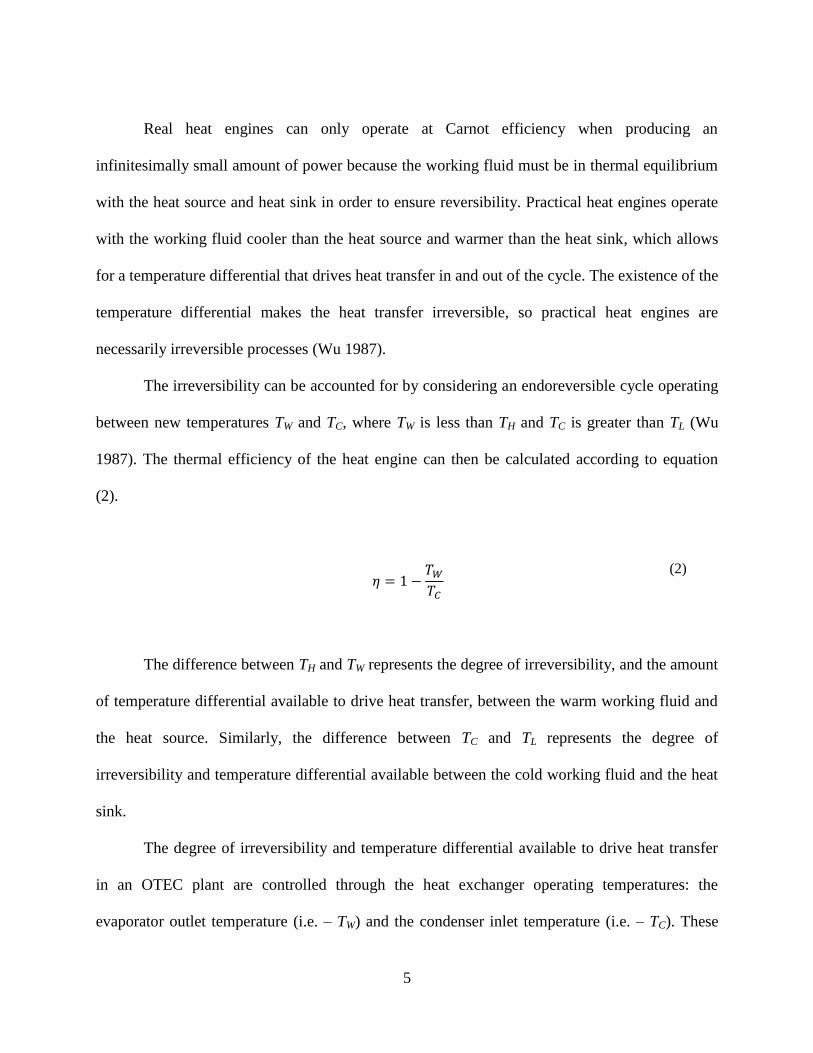
Real heat engines can only operate at Carnot efficiency when producing an

infinitesimally small amount of power because the working fluid must be in thermal equilibrium

with the heat source and heat sink in order to ensure reversibility. Practical heat engines operate

with the working fluid cooler than the heat source and warmer than the heat sink, which allows

for a temperature differential that drives heat transfer in and out of the cycle. The existence of the

temperature differential makes the heat transfer irreversible, so practical heat engines are

necessarily irreversible processes (Wu 1987).

The irreversibility can be accounted for by considering an endoreversible cycle operating

between new temperatures TW and TC, where TW is less than TH and TC is greater than TL (Wu

1987). The thermal efficiency of the heat engine can then be calculated according to equation

(2).

(2)

The difference between TH and TW represents the degree of irreversibility, and the amount

of temperature differential available to drive heat transfer, between the warm working fluid and

the heat source. Similarly, the difference between TC and TL represents the degree of

irreversibility and temperature differential available between the cold working fluid and the heat

sink.

The degree of irreversibility and temperature differential available to drive heat transfer

in an OTEC plant are controlled through the heat exchanger operating temperatures: the

evaporator outlet temperature (i.e. – TW) and the condenser inlet temperature (i.e. – TC). These

6

temperatures characterize the thermodynamic state of the working fluid at the turbine inlet and

outlet, and therefore the amount of useful work that can be extracted from the engine. Since there

are two temperatures, the irreversibility associated with heat transfer to the heat source and heat

sink can be controlled independently.

There exists a balance between the degree of irreversibility and the rate of heat transfer. If

the temperature difference between the working fluid and the heat source and sink is small, then

TW will be high and TC will be low. Equation (2) predicts that the efficiency of such a heat engine

is high, but the small temperature differential means that heat transfer rates will be low.

Conversely, if the temperature difference is high, the thermal efficiency of the heat engine is low

but the heat transfer rate is high. At either extreme, no power is produced. At the limit in which

the temperature difference is zero, an infinitesimally slow heat engine approaching the Carnot

efficiency exists. At the limit in which the temperature difference is maximized, thermal energy

is transferred directly from the heat source to the heat sink and no power is available for

extraction.

Between the two extremes of temperature difference selection exists an optimum choice

at which power output is maximized. Significant research has been conducted to determine the

optimum temperature difference considering the irreversibility required for a practical heat

engine. Following up on work by Curzon and Ahlborn (1975), Wu (1987) found a theoretical

bound for OTEC performance based on an endoreversible Carnot engine, and used the results to

predict optimum heat exchanger operating temperatures. Wu continued his work by extending

the analysis to an endoreversible Rankine engine (1989); finding that when maximizing the

amount of power produced per unit heat exchanger area, the optimum area ratio of heat

exchangers could be determined from the ratio of their heat transfer coefficients (1990, 1991);

7

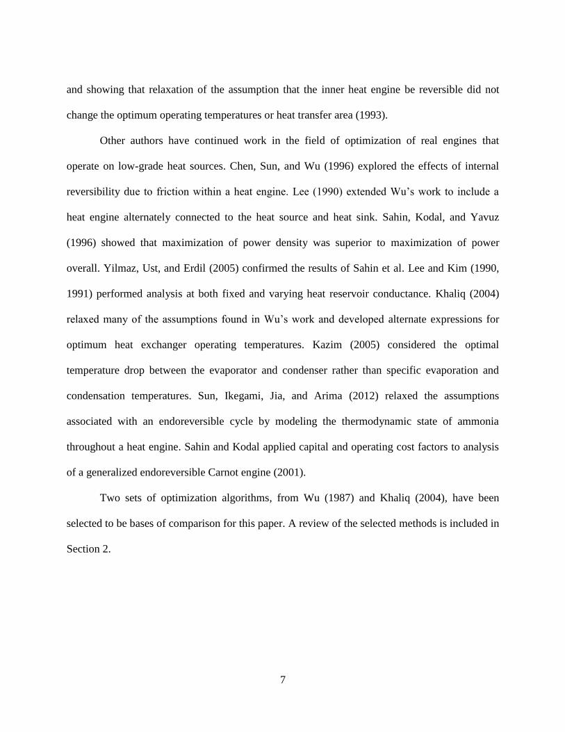
and showing that relaxation of the assumption that the inner heat engine be reversible did not

change the optimum operating temperatures or heat transfer area (1993).

Other authors have continued work in the field of optimization of real engines that

operate on low-grade heat sources. Chen, Sun, and Wu (1996) explored the effects of internal

reversibility due to friction within a heat engine. Lee (1990) extended Wu’s work to include a

heat engine alternately connected to the heat source and heat sink. Sahin, Kodal, and Yavuz

(1996) showed that maximization of power density was superior to maximization of power

overall. Yilmaz, Ust, and Erdil (2005) confirmed the results of Sahin et al. Lee and Kim (1990,

1991) performed analysis at both fixed and varying heat reservoir conductance. Khaliq (2004)

relaxed many of the assumptions found in Wu’s work and developed alternate expressions for

optimum heat exchanger operating temperatures. Kazim (2005) considered the optimal

temperature drop between the evaporator and condenser rather than specific evaporation and

condensation temperatures. Sun, Ikegami, Jia, and Arima (2012) relaxed the assumptions

associated with an endoreversible cycle by modeling the thermodynamic state of ammonia

throughout a heat engine. Sahin and Kodal applied capital and operating cost factors to analysis

of a generalized endoreversible Carnot engine (2001).

Two sets of optimization algorithms, from Wu (1987) and Khaliq (2004), have been

selected to be bases of comparison for this paper. A review of the selected methods is included in

Section 2.

8

1.2.2. Seawater Flow Rate

An OTEC plant must generate more power than is scheduled for export. An OTEC

system includes both seawater and working fluid pumps that require power to operate. The

power for these components must be generated by the OTEC plant in addition to the net power

that will be sold. The power required beyond net output is called parasitic power, and the sum of

net power and parasitic power is gross power. The relationship between OTEC gross power,

parasitic power, and net power is given in equation (11).

The largest component of OTEC parasitic power is seawater pumping. The expression to

calculate parasitic pumping power is shown in equation (3).

(3)

Neglecting the fact that the pressure differential, , is a function of seawater mass

velocity through the heat exchangers, parasitic pumping power is directly proportional to the

mass flow rate of seawater, . Therefore, all other factors being equal, an OTEC plant that uses

more seawater will need to produce more gross power than a plant that uses less seawater. The

increased gross power requires a larger, and more expensive, system.

1.2.3. Impact on OTEC Design

An efficient OTEC plant must balance the thermal efficiency of its underlying heat

engine, temperature differential available to drive heat transfer, and parasitic electrical loads. The

9

balance is achieved by selection of appropriate seawater flow rates and heat exchanger operating

temperatures. The fact that the life-cycle cost of OTEC is heavily dependent on capital costs

means that careful control of overall plant size is required for OTEC to be cost-competitive with

existing power production technologies.

10

2. LITERATURE REVIEW

OTEC optimization algorithms found in the literature make use of finite-time

thermodynamics, which is the study of endoreversible heat engines that relax the isothermal heat

transfer assumption inherent in the Carnot cycle. An overview of the concept underlying finite-

time thermodynamics was given in section 1.2.1. Such analysis allows researchers to consider

the thermal duty and power output from heat engines. Finite-time analysis is particularly

important in analyzing heat engines that operate on low-grade heat, as OTEC does, because a

significant portion of the available temperature difference must be allocated to heat transfer in

order to maintain sufficient power output. Two algorithms were selected from the literature for

comparison with the research presented in this paper.

The conclusions presented in the original work by Wu (1987) were not significantly

changed by subsequent analysis; later expressions for optimum heat exchanger operating

temperature evaluate to the same result even if their functional forms are different. Thus, Wu’s

original approach has been selected as a basis for comparison because it is representative of a

straight-forward approach. The method developed by Khaliq (2004) takes advantage of

advancements made by several prior researchers, and has been selected as the second basis for

comparison. Khaliq’s work relaxes many of the assumptions made by Wu, and presents

expressions for optimum heat exchanger operating temperature that evaluate to different results

compared to Wu’s method. Each algorithm is briefly presented below.

11

2.1. Isothermal Heat Reservoirs with a Carnot Engine

Wu (1987) considered a Carnot heat engine operating between temperatures TW and TC

such that TW is less than the temperature of the heat source, and TC is greater than the

temperature of the heat sink. Assuming the temperatures of the heat reservoirs are constant, the

amount of time required for heat transfer between the Carnot heat engine and the heat reservoirs

can be calculated from:

(4)

Where (T1 – T2) represents the temperature difference between one of the Carnot heat engine

operating temperatures and its associated heat reservoir temperature. Wu showed that the

optimum Carnot operating temperatures are:

(5)

(6)

Where:

(7)

12

The thermal efficiency of the Carnot heat engine is:

(8)

Wu’s work predicts the optimum operating temperatures and thermal efficiency of an

OTEC plant designed to produce the maximum possible amount of power. It addresses the heat

engine efficiency design challenge discussed in Section 1.2.1, but not the parasitic power

concerns from Section 1.2.2. In addition, the analysis makes some simplifying assumptions that

do not accurately reflect real OTEC systems. Section 2.1.1 below outlines the assumptions in

question.

2.1.1. Limiting Assumptions

Wu models the OTEC heat source and sink as isothermal entities. Therefore, the effects

of seawater temperature variation through the heat exchanger are neglected. This assumption

simplifies the analysis because the temperature difference driving heat transfer is simply the

difference between the temperature of the heat source or sink and the working fluid. Otherwise,

the log mean temperature difference (LMTD) would be required to compensate for the seawater

temperature variation. The fact that LMTD does not vary linearly with working fluid temperature

means that the assumption of an isothermal heat source and heat sink introduces inaccuracy into

the analysis.

Wu’s algorithm accounts for the thermodynamic effects finite-time heat transfer on heat

engine design, but makes broad assumptions regarding the seawater flow rates required to

13

operate the plant. The method requires a priori knowledge of the heat transfer coefficient and

total area of the heat exchangers. Since the heat transfer coefficient of an OTEC heat exchanger

is dependent on the mass velocity of seawater, fixing both heat transfer coefficient and heat

transfer area implicitly fixes seawater flow rate. Therefore, OTEC plant optimization in terms of

the relationship between gross power and net power is excluded.

In addition to its role in excluding the effects of parasitic power from the optimization

process, the assumption of a fixed heat transfer coefficient limits the capability of finite-time

thermodynamic OTEC optimization methods to account for the practical implications of using

heat exchangers. The heat transfer coefficient of a real heat exchanger varies as a function of the

mass velocity of seawater; high velocities result in high heat transfer coefficients and low

velocities result in low heat transfer coefficients. The heat exchanger can be operated anywhere

along a wide range of potential velocities. The fact that heat transfer coefficient is fixed in Wu’s

analysis restricts the optimization to a single operating point. Moreover, the analysis does not

include a method of evaluating whether the heat exchanger would perform better at a different

point. The quality of the optimization process is therefore partially dependent on the heat

exchanger designer’s ability to select an OTEC-appropriate operating point.

2.2. Heat Reservoirs with Varying Heat Capacity Rate and a Rankine Engine

Khaliq (2004) presented a comprehensive optimization scheme that modeled a Rankine

engine without the need for isothermal heat reservoirs. He also allowed the mass flow rate of

seawater (and therefore the heat capacity rate of the heat source and heat sink) to vary. These

14

modifications more accurately reflect the real OTEC heat source and heat sink, which must use a

finite amount of seawater to fuel the heat engine.

Khaliq’s work is an extension of Wu’s in that it also produced expressions for the

optimum evaporator and condenser operating temperatures. Khaliq relaxed the following

assumptions made in the derivation of equations (5) through (8): isothermal heat reservoirs,

constant heat conductance, and constant heat capacitance. Khaliq calculates the optimum

evaporator and condenser operating temperatures to be:

(9)

(10)

The heat engine thermal efficiency at maximum power output was found to be

independent of reservoir heat conductance, capacitance, or temperature variation, and equation

(8) is unchanged (Khaliq 2004). As with Wu’s work, Khaliq’s methods address heat engine

efficiency, but not parasitic power.

2.2.1. Limiting Assumptions

Unlike Wu, Khaliq includes the effects of seawater temperature variation and uses LMTD

in the derivation of equations (9) and (10). However, the analysis decouples heat transfer

15

coefficient from seawater flow rate, and therefore excludes the effects of parasitic power from

the optimization as discussed in section 2.1.1.

The fact that Khaliq allows independent variation in seawater flow rate introduces an

implicit assumption that the heat transfer coefficients of the heat exchangers are independent of

mass velocity of seawater through the heat exchanger. If the seawater flow rate varies, but the

heat exchanger area remains unchanged, then the mass velocity of seawater through the heat

exchanger must also change. A real heat exchanger responds to changes in mass velocity with

changes in heat transfer coefficient, but Khaliq’s analysis treats heat transfer coefficient and

mass velocity as independently varying quantities.

16

3. MODELING REAL OTEC SYSTEMS

The net power produced from an OTEC system can be described by:

(11)

Pgross represents the total power output of the OTEC plant. It is this value that published

OTEC optimization schemes have sought to maximize. However, Pparasitic is not trivial.

Preliminary modeling using the Makai OTEC Thermodynamic and Economic Model (MOTEM

– see Section 4) has shown that parasitic power losses can account for up to 40% of the total

electrical output of an OTEC plant. Minimization of parasitic losses cannot be carried out

independently of Rankine cycle optimization because seawater flow rate has a direct impact on

overall heat transfer coefficient, and therefore heat transfer area requirements. Both heat transfer

coefficient and heat exchanger area are explicitly shown in equation (7), and are found in the

derivation of equations (9) and (10).

3.1. Theoretical Magnification of the Effects of Variation in Optimization Parameters

When designing an OTEC plant for minimum heat exchanger size, the configuration is

sensitive to two pairs of operating parameters: evaporator and condenser operating temperatures,

and warm and cold seawater flow rates. The sensitivity stems from the fact that heat exchanger

performance is tied to seawater mass velocity through the heat exchanger and the mean

temperature difference available between the working fluid and the seawater.

17

A representative relationship between seawater velocity and the overall heat transfer

coefficient of a heat exchanger can be expressed as:

(12)

where C is some unknown positive constant. Assuming that the seawater flow rates of any

particular OTEC plant configuration are held constant, the mass velocity through the heat

exchanger is a function of the amount of heat exchanger over which seawater must be

distributed:

(13)

The amount of heat exchanger required can be calculated from:

(14)

Equations (12) through (14) can be combined to give a relation of the form:

(15)

Solving for U gives:

18

(16)

The effect of the magnification on heat transfer area can be determined by combining equations

(12) through (14) to eliminate U instead of A:

(17)

Solving for A gives:

(18)

For all C less than 1, equations (16) and (18) grow faster with increasing seawater flow

rate than do equations (12) and (14). Therefore, the change in overall heat transfer coefficient

and the change in heat transfer area due to a change in seawater flow rate in a real OTEC plant

are magnified. The physical rational for the magnification is as follows:

1. An increase in seawater mass flow rate causes an increase in seawater mass

velocity through the heat exchanger.

2. The increase in mass velocity causes an increase in overall heat transfer

coefficient.

19

3. At constant duty, the increased heat transfer coefficient allows for a reduced heat

transfer area.

4. The reduced heat transfer area further increases the mass velocity through the heat

exchanger.

5. The increased mass velocity causes an increase in overall heat transfer coefficient.

The relationship is further complicated by the fact that neither LMTD nor Q is fixed when

seawater flow rate varies. A change in seawater flow rate at constant duty will change the

seawater outlet temperature, which will change the LMTD. Changing seawater flow rate also

changes the pumping power required, which changes the thermal duty required.

At constant duty, an increase in seawater flow rate will increase the temperature at which

the warm seawater exits the evaporator or decrease the temperature at which the cold seawater

exits the condenser. In both cases, LMTD is increased. Since increased LMTD allows for reduced

heat exchanger area, the variability of LMTD with seawater flow further magnifies the cycle

described above. Since duty increases when seawater flow rate increases, and increased duty

requires more heat transfer area, the variability of Q with seawater flow counteracts the cycle

described above. The relative strength of the magnifying effects described above and the

counteracting effects of variation in Q depends on the performance curves of the specific heat

exchangers used. Table 2 shows an example of a case where variation in Q was sufficient to

completely counteract the magnification effect on heat transfer area, but not on heat transfer

coefficient.

The cycle described above also magnifies the effect of changes in LMTD due to changes

in heat exchanger operating temperature. Heat transfer area and LMTD are inversely related as

20

shown in equation (14). The change in area associated with a change in LMTD increases the

mass velocity of seawater through the heat exchanger. The increased mass velocity magnifies the

reduction in area as described above. The effect is captured in the fact that equation (18) is more

sensitive to changes in LMTD than is equation (14) for all C less than 1.

Equations (16) and (18) are undefined for C greater than or equal to 1. This captures the

fact that the magnification cycle diverges if overall heat transfer coefficient grows faster than a

linear function as mass velocity changes. The divergence arises because the relationship between

mass velocity and heat transfer area is linear when seawater flow rate and duty are held constant.

If the overall heat transfer coefficient grows faster than the heat transfer area shrinks, then the

two parameters can never balance. The limit that C be less than one is appropriate because real

heat exchangers exhibit diminishing returns in overall heat transfer coefficient as mass velocity

is increased, which ensures that the relationship between the two grows more slowly than a linear

relationship.

3.2. Magnification of the Effects of Optimization Parameter Variation in MOTEM

MOTEM was tested to determine if it captured the effects implied by equations (16) and

(18). To conduct the test, total thermal duty was artificially held constant and warm water flow

rate was increased 25%. As shown in equation (25), the value for C used in MOTEM for this

analysis is 0.5. Therefore, a 25% increase in evaporator heat transfer coefficient and a 25%

decrease in heat transfer area are predicted by equations (16) and (18).

21

Table 1: Magnification of the Effects of a 25% Increase in Warm Water Flow Rate at Fixed

Thermal Duty

The change in heat transfer coefficient is slightly higher than predicted by equation (16),

and the change in heat transfer area is slightly lower than predicted by equation (18). However,

the values are significantly higher than the 12% variation predicted by equations (12) and (14).

MOTEM accurately captures the effects of magnified responses to variation in optimization

parameters. In order to evaluate the relative importance of changes in pumping power due to

increased seawater head loss, a second test was conducted in which the constant thermal duty

assumption is relaxed.

Baseline +25% WW Flow % Variation

Gross Power Output 142.2 142.3 MW 0%

Net Power Output 100.0 100.0 MW

Warm Water Flow Rate 470,000 587,500 kg/s 25%

Cold Water Flow Rate 350,000 350,000 kg/s

Evaporator

Operating Temperature 21 21

Heat Transfer Area 350,171 273,243 m2 -22%

U-value 5.09 6.44 kW/m2/C 27%

Waterside Head Loss 18.6 18.6 kPa 0%

Condenser

Operating Temperature 9.6 9.6

Heat Transfer Area 254,914 256,721 m2 1%

U-value 5.15 5.13 kW/m2/C 0%

Waterside Head Loss 19.5 19.2 kPa -1%

22

Table 2: Magnification of the Effects of a 25% Increase in Warm Water Flow Rate with Variable

Thermal Duty

The 25% increase in warm water flow rate results in a 9% increase in gross power

requirements, which requires a 9% increase in thermal duty. The increased gross power is

required to compensate for the increased warm water flow rate and the increased evaporator

seawater head loss. The added thermal duty requires additional heat transfer area, and

counteracts the magnification effects. The counteraction is strong enough that heat transfer area

variation is smaller than that predicted by equation (14). However, the variation in overall heat

transfer coefficient is still greater than that predicted by equation (12). Additional condenser heat

transfer area is also required to accommodate the 9% increase in thermal duty. However, since

no additional cold water flow was provided, the magnification effect works in reverse; a large

increase in heat transfer area and a large decrease in overall heat transfer coefficient are

observed.

Baseline +25% WW Flow % Variation

Gross Power Output 142.2 155.1 MW 9%

Net Power Output 100.0 100.0 MW

Warm Water Flow Rate 470,000 587,500 kg/s 25%

Cold Water Flow Rate 350,000 350,000 kg/s

Evaporator

Operating Temperature 21 21

Heat Transfer Area 350,171 324,014 m2 -7%

U-value 5.09 5.91 kW/m2/C 16%

Waterside Head Loss 18.6 34.0 kPa 82%

Condenser

Operating Temperature 9.6 9.6

Heat Transfer Area 254,914 344,746 m2 35%

U-value 5.15 4.43 kW/m2/C -14%

Waterside Head Loss 19.5 10.7 kPa -45%

23

The differences between Table 1 and Table 2 indicate that the constant thermal duty

assumption is not valid when optimizing real OTEC systems. Variation in seawater head loss has

a significant impact on heat exchanger thermal duty. Full OTEC system simulation is required in

order to accurately predict the interaction between mass velocity through the heat exchanger,

total thermal duty, heat transfer area, and overall heat transfer coefficient.

24

4. THE OTEC MODEL

As part of an SBIR research grant from the Office of Naval Research beginning in 2007,

Makai Ocean Engineering developed an OTEC computer model capable of simulating a steady-

state OTEC plant. The program is called the Makai OTEC Thermodynamic and Economic

Model (MOTEM). MOTEM includes a complete calculation of the thermodynamic state of the

working fluid throughout out the system, as well as modeled heat exchanger performance curves

that account for the effects of varying seawater flow rate and seawater temperature.

Makai agreed to permit use of MOTEM as part of the research presented in this paper. As

a condition of the permission, the economic analysis modules were disabled and the optimization

was carried out to minimize total heat exchanger area. Minimization of heat exchanger area is a

good approximation of economic optimization because it captures both heat exchanger costs and

cost for space as discussed in Section 1.2.

4.1. An OTEC Simulator

MOTEM is not an OTEC optimization algorithm, but an OTEC simulation program. It is

comprised of modules that represent components or processes in a practical OTEC plant design.

A subset of the modules includes heat exchanger performance modeling, Rankine cycle

modeling, overall system hydraulics, and cold water pipe hydraulics.

The most important modules are the Rankine cycle performance and heat exchanger

performance modules, and an overview of each is provided in Sections 4.2 and 4.4. The user is

able to input a wide variety of technical parameters, the most important of which include desired

net power output, seawater flow rates, heat exchanger operating temperatures, cold water pipe

25

diameter, and seawater ducting geometry. MOTEM will then calculate the amount of heat

exchanger area required to produce the desired net power. It will also inform the user if the input

parameters cannot produce the desired result. In an alternative mode, the user provides the heat

transfer area for the evaporator and the condenser instead of the desired net power. MOTEM

then calculates the net power output of the plant. If no net power can be produced, the program

will inform the user that the input configuration is not valid.

In addition to the technical calculations, MOTEM includes an economic evaluation

module. This module estimates the total capital cost of an OTEC plant based on the technical

parameters calculated by rest of the program.

The OTEC optimization algorithm is an automatic input manipulation system. It modifies

the inputs over a user-specified solution space to find the configuration that minimizes OTEC

plant total capital cost. Since the economic module of MOTEM was disabled for this analysis,

the optimization algorithm was modified to converge on minimum heat transfer area. An

overview of the optimization algorithm is provided in Section 5. Since MOTEM’s optimization

process is carried out based on a full OTEC simulation, it achieves the best possible

configuration within the accuracy of the simulation and the limits of the optimization algorithm.

It can therefore be used as a benchmark against which other optimization algorithms are

compared.

4.2. Governing Equations

MOTEM is based on an energy balance on three fluids: warm seawater, cold seawater,

and the working fluid. The rate at which energy leaves the warm seawater must equal the rate at

26

which energy enters the working fluid in the evaporator. Similarly, the rate at which energy

leaves the working fluid in the condenser must equal the rate at which energy enters the cold

seawater. The rate at which energy enters and leaves the working fluid is shown in equation (19),

and the rate at which energy leaves the warm seawater and enters the cold seawater is shown in

equation (20).

(19)

(20)

MOTEM adjusts the heat transfer area in equation (19) until the calculated duty matches

that from equation (20). The changes in heat transfer area cause changes in the mass velocity of

the seawater through the heat exchangers, and therefore the heat transfer coefficient, as discussed

in section 3.1. The relationship between the rate of energy transfer to and from the working fluid

and the power output of the system is based on the thermodynamic state of the working fluid in

the heat engine. The output of the turbine is calculated from Equation (21).

(21)

The specific enthalpy of the working fluid at the turbine inlet and outlet are calculated in

the Rankine cycle modeling module, which is discussed in section 4.3. The mass flow rate of the

working fluid is calculated from the working fluid heat of vaporization according to equation

27

(22). The thermal duty calculated in equations (19), (20), and (22) are balanced independently

for the evaporator and the condenser.

(22)

The net power output is calculated according to equation (11). The parasitic power is

calculated based on the seawater pumping power and the working fluid pumping power required.

The working fluid pumping power is calculated from the thermodynamic state of the working

fluid in the heat engine according to equation (23).

(23)

The seawater pumping power is calculated based on the head loss calculated over the

entire seawater flow path, as shown in equation (24).

(24)

MOTEM adjusts the working fluid flow rate, and therefore the thermal duty required of

the heat exchangers, until the net power reaches the user-specified target value. In doing so,

equations (19) through (24) are solved iteratively and simultaneously until the heat balance

equations match.

28

4.3. Rankine Cycle Modeling

The heat engine modeled within MOTEM is a Rankine cycle. The cycle is calculated in

an iterative table. Each entry in the table represents a node in the cycle. Each node represents the

inlet or outlet of one of the system components. Figure 2 shows a power cycle diagram that

includes the temperature, pressure, and quality at each node within the thermodynamic cycle

model.

29

Figure 2: Power Cycle Diagram Showing Each Node in the OTEC Model’s Thermodynamic Cycle

De-mister: -45 m Turbine (Datum): 0 m

P = 884 kPa P = 879 kPa P = 869 kPa P = 608 kPa

T = 21.0 C T = 20.8 C T = 20.4 C T = 9.7 C

X = 65% X = 100% Length = 55 m X = 100% X = 97%

Diameter = 2.30m

Length = 5 m P = 879 kPa Flow Rate = 3929 kg/s

Diameter = 2.83m T = 21.0 C Length = 75 m

Flow Rate = 6045 kg/s X = 0% Diameter = 2.68m

Flow Rate = 3929 kg/s

Length = 2 m

Diameter = 0.76m


P = 891 kPa P = 608 kPa

P = 885 kPa T = 21.0 C T = 9.6 C

T = 21.0 C X = 0.00 X = 97%

X = 65% Water Tin = 4.1 C

Water Tin = 25.7 C Holding Tank: -47 m Condenser: -65 m Water Flow = 350000 kg/s

Water Flow = 470000 kg/s Evaporator: -47 m Water Tout = 7.4 C

Water Tout = 23.1 C P = 891 kPa P = 607 kPa

P = 907 kPa T = 21.0 C T = 9.6 C

T = 13.7 C X = 0% X = 0%

X = 0%

Length = 38 m Length = 10 m

Diameter = 0.76m Diameter = 1.01m

Flow Rate = 2116 kg/s Flow Rate = 3929 kg/s

P = 1053 kPa

T = 21.1 C P = 636 kPa

Length = 38 m X = 0% T = 9.6 C

Diameter = 1.26m X = 0%

Flow Rate = 6045 kg/s Recirc Pump: -75 m

Buffer: -70 m

P = 1083 kPa

T = 21.1 C P = 636 kPa

X = -3% T = 9.6 C

X = 0%

Length = 5 m

Diameter = 0.76m


Length = 10 m

P = 1082 kPa Diameter = 1.01m

T = 21.1 C Flow Rate = 3929 kg/s

X = 0%

Feed Pump: -75 m

Pump Wye: -75 m

P = 1082 kPa P = 1088 kPa P = 662 kPa

P = 1080 kPa T = 9.7 C T = 9.7 C T = 9.6 C

T = 13.7 C X = 0% Length = 5 m X = -8% X = 0%

X = 0% Diameter = 1.01m


30

The complete thermodynamic state of the working fluid is calculated at each node, which

allows convenient calculation of turbine power output and pump power input (see section 4.2).

The iteration algorithm uses the evaporator outlet temperature and the condenser inlet

temperature as inputs. Saturated conditions are assumed at these points, so the thermodynamic

state of the working fluid is fully defined. The state of the working fluid is calculated throughout

the rest of the system based on the following methods:

1. The pressure drop between adjacent nodes is calculated from the Darcy-Weisbach

equation, with the friction factor calculated with the Swamee-Jain equation.

2. Energy extraction at the turbine is assumed to be isentropic.

3. Energy input at pumps is assumed to be isentropic.

4. Pressure losses are assumed to be isentropic for vapor.

5. Pressure losses are assumed to occur at constant density for liquid.

6. Fluid properties are calculated using the equation-of-state program REFPROP 7

from the National Institute of Standards and Technology

The above statements provide two thermodynamic parameters for each node in the

system (i.e. – pressure and entropy for vapor nodes; pressure and density for liquid nodes).

Therefore, the thermodynamic state of the working fluid can be calculated everywhere. Iterative

calculations are required because the pressure drop between nodes on the system is a function of

working fluid flow rate. Working fluid flow rate is dependent on the specific work extracted by

the turbine, which is in turn dependent on the thermodynamic state at the turbine inlet and outlet.

31

An acknowledged limitation of MOTEM’s thermodynamic modeling scheme is that it

does not fully account for component inefficiencies. Turbine and pump wire-to-fluid efficiencies

are included in the power calculations, but not in the Rankine cycle calculations. Therefore, there

is a mismatch between the amount of thermal energy extracted from the working fluid and the

power output (input) of the turbine (pumps). This essentially models all inefficiencies as

electrical in nature – the energy is lost to the environment as waste heat. However, some of the

inefficiency is hydraulic. Such inefficiencies add entropy to the working fluid, and this entropy

addition is not captured by the Rankine cycle model. In a real system, the excess energy would

be rejected at the condenser, so MOTEM under-predicts condenser thermal duty. However, the

inefficiency operates on the extracted energy of the plant, which is less than 4% of the thermal

duty. Even if 25% of the energy assumed to be extracted from the Rankine cycle is instead

converted into entropy, it would account for less than 1% of the condenser thermal duty.

4.4. Heat Exchanger Modeling

A thermodynamic description of a Rankine cycle is not sufficient to accurately simulate

OTEC plant operation. Heat exchanger performance is integrally related to OTEC plant

performance; it affects parasitic power losses, optimum water flow rates, and optimum operating

temperatures.

As part of its OTEC development program, Makai Ocean Engineering has acquired heat

performance curves for a brazed-fin OTEC evaporator and a twisted tube shell-and-tube OTEC

condenser. The curves include relations for overall heat transfer coefficient, working fluid head

32

loss, and seawater head loss. The curves parameterize performance based on seawater and

working fluid velocities.

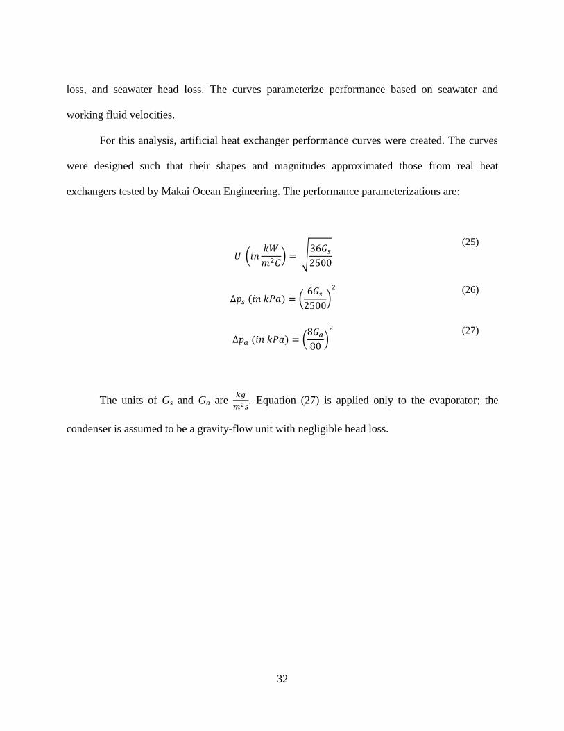
For this analysis, artificial heat exchanger performance curves were created. The curves

were designed such that their shapes and magnitudes approximated those from real heat

exchangers tested by Makai Ocean Engineering. The performance parameterizations are:

(25)

(26)

(27)

The units of Gs and Ga are

. Equation (27) is applied only to the evaporator; the

condenser is assumed to be a gravity-flow unit with negligible head loss.

33

5. OPTIMIZATION ALGORITHMS

The ultimate goal of MOTEM is to allow rapid optimization of varying OTEC plant

configurations in order to minimize capital cost.

5.1. MOTEM’s Optimization Algorithm

MOTEM uses a variation on the path of steepest descent optimization scheme. The path

of steepest descent involves a sensitivity analysis in which the optimized variable is perturbed

above and below its initial value. The direction that results in the largest decrease in the objective

parameter is selected as the new value for the optimized variable. The process is repeated until

all perturbations result in an increase in the objective parameter. Such an optimization scheme is

considered crude and can be inefficient, but is easy to implement (Press, Flannery, Teukolsky &

Vetterling, 1997). MOTEM makes use of a multi-dimensional form of the path of steepest

descent. Seawater flow rates and heat exchanger operating temperatures are simultaneously

varied, and the combination of parameters that results in the smallest optimization parameter

value (i.e. – minimum heat transfer area) is selected as the new set of values.

The primary difficulty with the path of steepest descent is that the steepest path at any

given point in the solution space may not point towards the minimum value. The steepest path

will generally only point towards the minimum value if the principal optimization direction is

parallel to one of the available optimization directions (i.e. – the path to the minimum value

involves changes in only one of the available optimization parameters). In the worst case

scenario, where the steepest path points as far away from the actual minimum value as possible,

the method of steepest descent degenerates to a series of perpendicular optimization steps in

34

which each step is equally oblique to the path that points toward so the minimum value (Press et

al., 1997). The result is that the method of steepest descent is sensitive to the initial values of the

optimization parameters, and can require extensive computation resources if the principal

directions are far from the available optimization directions. MOTEM deals with this fact by

limiting the number of varying parameters in any given optimization step (see section 5.2).

A superior method of optimization would be the Fletcher-Reeves conjugate gradient

algorithm. Conjugate gradient algorithms are analogous to the method of steepest descent, but

focus on conjugate directions rather than the direction with maximum gradient. A conjugate

direction is an optimization path that does not counteract the effects of the path from the previous

iteration. In the worst case scenario of the method of steepest descent, each iteration step

operates against the gradient of the previous step to some degree – it reverses some of the

optimization already completed. Optimization along a path conjugate to the previous path would

ensure that the gradient along the previous optimization path stays at zero, which maintains the

previous optimization gains (Press et al., 1997). In essence, the Fletcher-Reeves method favors

conjugate optimization directions over the path of steepest descent, and tends to converge in

fewer iteration steps.

5.2. Robustness of the Optimization Scheme

A significant challenge in the field of optimization algorithm design is distinguishing

between local and global minima. A global minimum is the point on an optimization surface

where the objective variable is at its minimum value over the entire domain. A local minimum is

a point at which the objective variable is at a minimum value relative to a nearby locus of points,

35

but not relative to the entire domain (Press et al., 1997). A robust optimization scheme must be

able to recognize local minima and continue iterating until the global minimum is found.

The surface over which MOTEM optimizes does not have any local minima. Figure 9,

Figure 10, Figure 12, and Figure 13 show that the derivative of the linear optimization curve for

each optimization variable is monotonically increasing. A function with a monotonic derivative

has no local extrema – only a global extrema. Additionally, a linear combination of orthogonal

functions with monotonic derivatives has no local extrema. Therefore, it is not expected that the

overall four-dimensional surface, which is comprised of component functions with monotonic

derivatives, will have local minima. This expectation was tested early in MOTEM’s development

by creating a global optimization map over a wide range of seawater flow rates and heat

exchanger operating temperatures. The test confirmed that local minima do not exist.

5.3. Solution Space Reduction

Two separate optimization categories are considered: heat exchanger operating

temperature and seawater flow rate. Heat exchanger operating temperature refers to the

saturation temperature of the working fluid at the evaporator outlet and the condenser inlet.

These temperatures control the mean temperature difference across the heat exchanger (and

therefore total heat transfer rate) as well as the thermal efficiency of the Rankine cycle (and

therefore net power output). There are a total of four optimization parameters: evaporator outlet

temperature, condenser inlet temperature, warm seawater flow rate, and cold seawater flow rate.

Calculation of every possible combination of optimization parameters results in a number

of computations scaling as n4, where n is the number of allowable values for each parameter.

36

Addition of further optimization parameters will increase the exponent. MOTEM is intended to

operate over a large space of potential temperatures and water flows, and exponential growth of

the solution space requires more computational speed than is conveniently available. Therefore,

MOTEM was designed to optimize pairs of operating conditions. Each pair is optimized

together, resulting in a solution set of n2 for each pair. The total number of computations

therefore scales at n2 + n

2, and addition of further optimization parameters will result in

polynomial growth of the solution space. It is recognized that splitting the optimization

parameters into pairs is suboptimum, as some of the overlooked combinations could represent

superior configurations, but the compromise was deemed worthwhile in light of the improved

optimization resolution that is permitted.

5.4. Optimization of Operating Temperature

Figure 3 shows a sample optimization curve for the evaporator operating temperature.

Although MOTEM optimizes both evaporator and condenser operating temperatures

simultaneously, only a single parameter is shown for clarity.

37

Figure 3: Optimization Curve for Evaporator Operating Temperature

Any deviation from the MOTEM-predicted optimum temperature results in an increase in

the total heat transfer area required to produce 100 MW of electricity. The curve is steeper as

operating temperature increases. This trend is mirrored on condenser operating temperature

optimization curves; total heat transfer area required increases more steeply as condenser

operating temperature falls. In both cases, the increased sensitivity is found when the operating

temperature approaches the corresponding seawater temperature. As operating temperature and

seawater temperature converge, each incremental increase in operating temperature makes up a

larger percentage of the remaining temperature difference with the seawater. Therefore,

temperature difference falls proportionally faster as the operating temperature moves towards the

seawater temperature. A faster change in temperature difference results in a faster change in heat

transfer area requirements.

Normalized optimization curves are useful in comparing the effects of changes in

evaporator operating temperature to those in condenser operating temperature. Additionally,

0

100,000

200,000

300,000

400,000

500,000

600,000

700,000

800,000

900,000

1,000,000

19.0 19.5 20.0 20.5 21.0 21.5 22.0 22.5 23.0

To

tal H

eat

Tra

nsf

er A

rea

(m

2)

Evaporator Operating Temperature (C)

38

normalized curves divorce the analysis from the specific plant size modeled. Figure 4 is the

normalized optimization curve produced from Figure 3. All subsequent operating temperature

optimization curves in this paper will be normalized.

Figure 4: Normalized Optimization Curve for Evaporator Operating Temperature

The temperature variation is referred to a baseline value – the optimum temperature

predicted by MOTEM. Similarly, the heat transfer area is referred to the minimum value found at

the MOTEM-predicted optimum.

5.5. Optimization of Water Flow

Figure 5 shows a sample optimization curve for the cold water flow rate.

0%

5%

10%

15%

20%

25%

30%

35%

40%

45%

50%

-2.0 -1.5 -1.0 -0.5 0.0 0.5 1.0 1.5 2.0

Hea

t T

ran

sfer

Are

a V

ari

ati

on

Temperature Variation (C)

39

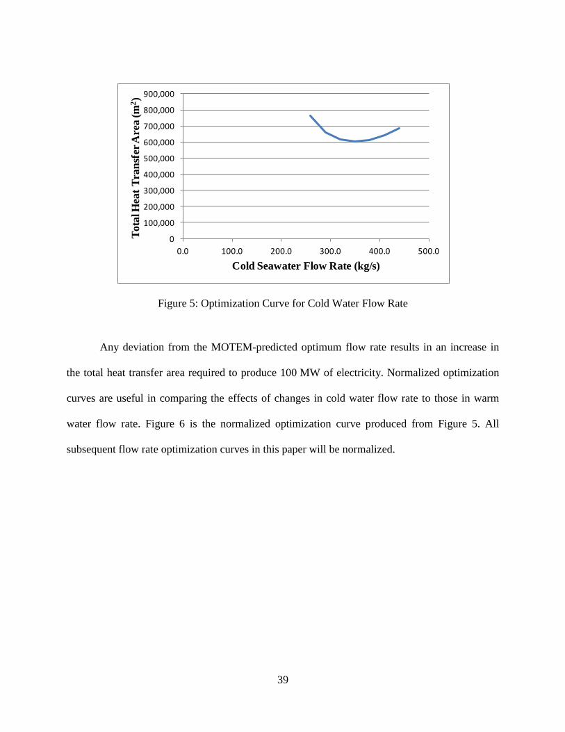
Figure 5: Optimization Curve for Cold Water Flow Rate

Any deviation from the MOTEM-predicted optimum flow rate results in an increase in

the total heat transfer area required to produce 100 MW of electricity. Normalized optimization

curves are useful in comparing the effects of changes in cold water flow rate to those in warm

water flow rate. Figure 6 is the normalized optimization curve produced from Figure 5. All

subsequent flow rate optimization curves in this paper will be normalized.

0

100,000

200,000

300,000

400,000

500,000

600,000

700,000

800,000

900,000

0.0 100.0 200.0 300.0 400.0 500.0

To

tal H

eat

Tra

nsf

er A

rea

(m

2)

Cold Seawater Flow Rate (kg/s)

40

Figure 6: Normalized Optimization Curve for Cold Seawater Flow Rate

The flow rate variation is referred to a baseline value – the optimum flow predicted by

MOTEM. Similarly, the heat transfer area is referred to the minimum value found at the

MOTEM-predicted optimum. The scale of all optimization curves is left constant throughout the

paper in order to facilitate comparison of the relative importance of each optimization parameter.

0%

5%

10%

15%

20%

25%

30%

35%

40%

45%

50%

-30% -20% -10% 0% 10% 20% 30%

Hea

t T

ran

sfer

Are

a V

ari

ati

on

Cold Seawater Flow Rate Variation

41

6. OPTIMIZATION RESULTS

Investigation of the optimization curves produced by MOTEM can reveal the relative

importance of the four optimization parameters. Although the optimization is carried out in pairs,

the performance curves are presented for individual parameters for the sake of clarity.

6.1. Temperature Optimization

Figure 7 and Figure 8 show the optimization curves for evaporator and condenser

operating temperatures.

Figure 7: Normalized Optimization Curve for Evaporator Operating Temperature

0%

5%

10%

15%

20%

25%

30%

35%

40%

45%

50%

-2.0 -1.5 -1.0 -0.5 0.0 0.5 1.0 1.5 2.0

Hea

t T

ran

sfer

Are

a V

ari

ati

on


42

Figure 8: Normalized Optimization Curve for Condenser Operating Temperature

The heat transfer area variation in Figure 7 is greater than that in Figure 8, thus

evaporator operating temperature is more important than condenser operating temperature for the

same variation. A technical description of the optimum OTEC plant configuration is shown in

Table 7 (in Section 7.1). The table shows that the LMTD in the optimum configuration is 2.7o C

for the evaporator and 3.6o C for the condenser. The smaller LMTD for the evaporator means that

any incremental change in evaporator operating temperature constitutes a proportionally larger

portion of the remaining temperature difference than does an incremental change in condenser

operating temperature. The condenser LMTD is larger than that of the evaporator because cold

water must be drawn up a pipe, while warm water is readily available. See the Section 7.1.2 for

details.

Figure 9 and Figure 10 show the effect of seawater flow rate reoptimization on the

operating temperature optimization curves. To produce the curves, MOTEM was allowed to

reoptimize the seawater flow rates (i.e. – find the warm and cold seawater flow rates that

0%

5%

10%

15%

20%

25%

30%

35%

40%

45%

50%

-2.0 -1.5 -1.0 -0.5 0.0 0.5 1.0 1.5 2.0

Hea

t T

ran

sfer

Are

a V

ari

ati

on


43

minimize the heat transfer area requirement) for each evaporator or condenser operating

temperature included in the figure.

Figure 9: Normalized Optimization Curve for Evaporator Operating Temperature with

Reoptimized Seawater Flow

0%

5%

10%

15%

20%

25%

30%

35%

40%

45%

50%

-2.0 -1.5 -1.0 -0.5 0.0 0.5 1.0 1.5 2.0

Hea

t T

ran

sfer

Are

a V

ari

ati

on


Unchanged Water Flow

Reoptimzed Water Flow

44

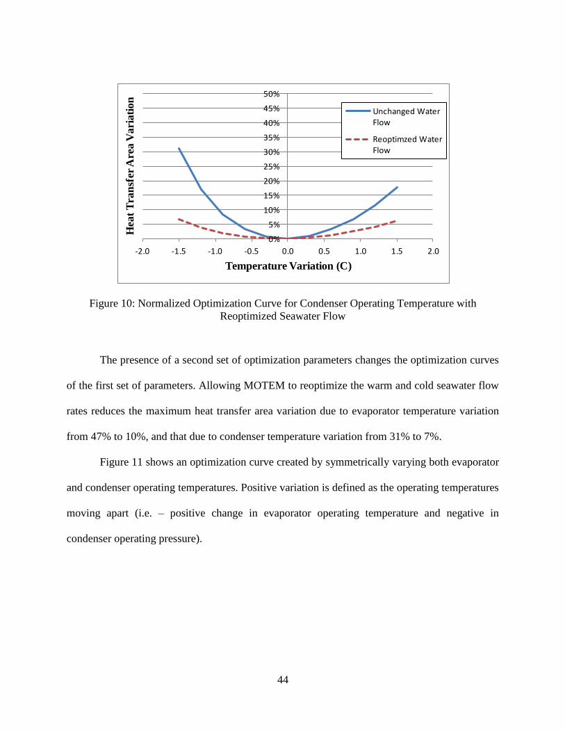
Figure 10: Normalized Optimization Curve for Condenser Operating Temperature with

Reoptimized Seawater Flow

The presence of a second set of optimization parameters changes the optimization curves

of the first set of parameters. Allowing MOTEM to reoptimize the warm and cold seawater flow

rates reduces the maximum heat transfer area variation due to evaporator temperature variation

from 47% to 10%, and that due to condenser temperature variation from 31% to 7%.

Figure 11 shows an optimization curve created by symmetrically varying both evaporator

and condenser operating temperatures. Positive variation is defined as the operating temperatures

moving apart (i.e. – positive change in evaporator operating temperature and negative in

condenser operating pressure).

0%

5%

10%

15%

20%

25%

30%

35%

40%

45%

50%

-2.0 -1.5 -1.0 -0.5 0.0 0.5 1.0 1.5 2.0

Hea

t T

ran

sfer

Are

a V

ari

ati

on




45

Figure 11: Normalized Optimization Curve for Simultaneous Variation of Evaporator and

Condenser Operating Temperature with Reoptimized Seawater Flow

When both evaporator and condenser operating temperatures are varied symmetrically,

the total variation in heat transfer area is smaller than that when only one temperature is varied.

Furthermore, reoptimization of water flow rates has only a minimal effect. See Section 6.3 for a

discussion on the implications of the conditional insensitivity of heat transfer area to water flow

optimization.

6.2. Water Flow Optimization

Figure 12 and Figure 13 show the optimization curves for seawater, both with and

without reoptimized operating temperatures.

0%

5%

10%

15%

20%

25%

30%

35%

40%

45%

50%

-2.0 -1.5 -1.0 -0.5 0.0 0.5 1.0 1.5 2.0

Hea

t T

ran

sfer

Are

a V

ari

ati

on




46

Figure 12: Normalized Optimization Curve for Warm Seawater Flow Rate with Reoptimized

Operating Temperatures

Figure 13: Normalized Optimization Curve for Cold Seawater Flow Rate with Reoptimized

Operating Temperatures

The effects of variation in warm water flow rate and cold water flow rate are comparable.

Allowing MOTEM to reoptimize heat exchanger operating temperatures reduced the maximum

0%

5%

10%

15%

20%

25%

30%

35%

40%

45%

50%

-30% -20% -10% 0% 10% 20% 30%

Hea

t T

ran

sfer

Are

a V

ari

ati

on

Seawater Flow Rate Variation

Unchanged Operating Temperatures

Reoptimzed Operating Temperatures

0%

5%

10%

15%

20%

25%

30%

35%

40%

45%

50%

-30% -20% -10% 0% 10% 20% 30%

Hea

t T

ran

sfer

Are

a V

ari

ati

on

Seawater Flow Rate Variation

Unchanged Operating Temperatures

Reoptimzed Operating Temperatures

47

heat transfer area variation from 9% to 2% in the warm water optimization curve, and from 26%

to 7% in the cold water optimization curve.

6.3. Heat Transfer Coefficient Ratio

Figure 11 shows that seawater flow rate optimization does not significantly reduce the

total heat transfer area when the heat exchanger operating temperatures deviate symmetrically

from optimum values (i.e. – evaporator operating temperature increases while condenser

operating temperature decreases, and vice versa). This is in contrast to the trend seen in Figure 9,

Figure 10, and Figure 12, where seawater flow optimization reduces heat transfer area variation

by a factor of 4. This implies that heat exchanger operating temperature optimization and

seawater flow rate optimization are not independent processes, and that there exists some

relationship between them that is unchanged when heat exchanger operating temperatures are

varied symmetrically.

To investigate the relationship, data tables were created that showed the main OTEC

characteristics along the entirety of the optimization curves. Table 3 shows a sample of the data

tables created. Review of the data revealed that the ratio of evaporator to condenser heat transfer

coefficient can be correlated with the level of seawater flow optimization. Table 4 shows the heat

transfer coefficient ratios for the simulations considered. The simulation case names identify

which heat exchanger operating temperature is allowed to vary, and whether seawater

reoptimization was allowed. Symmetric variation refers to mirrored variation in both evaporator

and condenser operating temperatures; an increase in evaporator temperature is associated with a

decrease in condenser temperature, and vice versa.

48

Table 3: Sample of OTEC Plant Characteristic Data

Table 4: Ratio of Evaporator Heat Transfer Coefficient to Condenser Heat Transfer Coefficient with Artificial Heat Exchangers

-1.5 -1.2 -0.9 -0.6 -0.3 Baseline 0.3 0.6 0.9 1.2 1.5

Gross Power Output 142.6 142.5 142.5 142.4 142.2 142.2 142.1 142.2 142.4 142.8 143.4 MW

Net Power Output 100.0 100.0 100.0 100.0 100.0 100.0 100.0 100.0 100.0 100.0 100.0 MW

Warm Water Flow Rate 470,000 470,000 470,000 470,000 470,000 470,000 470,000 470,000 470,000 470,000 470,000 kg/s

Cold Water Flow Rate 350,000 350,000 350,000 350,000 350,000 350,000 350,000 350,000 350,000 350,000 350,000 kg/s

Rakine Cycle Efficiency 3.1% 3.2% 3.3% 3.4% 3.5% 3.6% 3.7% 3.8% 3.9% 4.0% 4.1%

Evaporator

Operating Temperature 19.5 19.8 20.1 20.4 20.7 21.0 21.3 21.6 21.9 22.2 22.5

Heat Transfer Area 286,089 292,376 301,101 312,914 328,800 350,171 379,362 420,044 478,751 567,659 712,029 m2

U-value 5.63 5.57 5.49 5.38 5.25 5.09 4.89 4.65 4.35 4.00 3.57 kW/m2/C

Thermal Duty 5,628 5,456 5,292 5,138 4,992 4,855 4,728 4,611 4,504 4,409 4,325 MW

LMTD 3.49 3.35 3.20 3.05 2.89 2.72 2.55 2.36 2.16 1.94 1.70 C

Seawater Head Loss 27.9 26.7 25.2 23.3 21.1 18.6 15.9 12.9 10.0 7.1 4.5 kPa

Condenser

Operating Temperature 9.6 9.6 9.6 9.6 9.6 9.6 9.6 9.6 9.6 9.6 9.6

Heat Transfer Area 441,182 389,788 347,011 311,099 280,722 254,914 232,936 214,288 198,476 185,209 174,223 m2

U-value 3.910 4.160 4.410 4.660 4.900 5.147 5.380 5.610 5.830 6.040 6.230 kW/m2/C

Thermal Duty 5,446 5,274 5,111 4,956 4,811 4,675 4,548 4,431 4,324 4,228 4,144 MW

LMTD 3.16 3.25 3.34 3.42 3.49 3.56 3.63 3.68 3.74 3.78 3.82 C

Seawater Head Loss 6.5 8.3 10.5 13.1 16.1 19.5 23.3 27.6 32.2 36.9 41.7 kPa

Evaporator Temperature Variation

Simulation Case -1.5 -1.2 -0.9 -0.6 -0.3 Baseline 0.3 0.6 0.9 1.2 1.5 C

Evaporator Variation without Reoptimization 1.44 1.34 1.24 1.15 1.07 0.99 0.91 0.83 0.75 0.66 0.57

Evaporator Variation with Reoptimization 0.97 0.98 0.98 0.98 1.00 0.99 0.97 0.98 0.98 1.00 1.01

Symmetric Variation without Reoptimization 1.03 1.02 1.01 1.00 0.99 0.99 0.98 0.98 0.97 0.96 0.95

Temperature Variation

49

The ratio of evaporator to condenser heat transfer coefficient is uniform for the

reoptimized case and for the symmetric variation case, but changes significantly in the

unoptimized case. This implies that any configuration in which the heat transfer coefficient ratio

matches that in the optimized configuration is fully optimized for the specific heat exchanger

operating temperatures; no further heat transfer area reduction is possible by changing the

seawater flow rates. The fact that the ratio is constant when no further reduction in heat transfer

area is possible implies that it plays a role in OTEC plant optimization.

The calculation of evaporator to condenser heat transfer ratio was repeated with real

world heat exchangers, and cases in which the heat exchanger operating temperatures were

manipulated to maintain constant heat transfer coefficient ratio were added. In the added cases,

the evaporator operating temperature was varied identically with all other cases while the

condenser operating temperature variation was selected such that the heat transfer ratio was

approximately equal to that in the baseline case. If the heat transfer coefficient ratio is a metric

for level of optimization, then seawater reoptimization of the constant ratio cases will not result

in a reduction in heat transfer area requirements. Table 5 shows the heat transfer coefficient

ratios for the cases considered with real world heat exchangers.

The simulation case names identify which heat exchanger operating temperature is

allowed to vary, and whether seawater reoptimization was allowed. Symmetric variation refers to

mirrored variation in both evaporator and condenser operating temperatures; an increase in

evaporator temperature is associated with a decrease in condenser temperature, and vice versa.

Constant ratio refers to an evaporator variation that matches the values along the top of the table,

and a condenser variation selected to maintain a constant ratio between the evaporator and

condenser heat transfer coefficients.

50

Table 5: Ratio of Evaporator Heat Transfer Coefficient to Condenser Heat Transfer Coefficient with Real World Heat Exchangers

Simulation Case -1.5 -1.2 -0.9 -0.6 -0.3 Baseline 0.3 0.6 0.9 1.2 1.5

Evaporator Only without Reoptimization 2.34 2.14 1.95 1.78 1.61 1.45 1.30 1.15 1.00 0.84 0.68

Evaporator Only with Reoptimization 1.42 1.41 1.44 1.45 1.44 1.45 1.45 1.44 1.45 1.44 1.48

Symmetric without Reoptimization 1.66 1.61 1.57 1.53 1.49 1.45 1.41 1.37 1.32 1.26 1.19

Symmetric with Reoptimization 1.45 1.44 1.43 1.44 1.45 1.45 1.44 1.44 1.44 1.47 1.48

Constant Ratio without Reoptimization 1.47 1.46 1.44 1.46 1.46 1.45 1.46 1.46 1.46 1.47 1.48

Constant Ratio with Reoptimization 1.45 1.44 1.45 1.46 1.46 1.45 1.46 1.46 1.48 1.46 1.48

Temperature Variation [C]

51

All reoptimized cases maintain the same heat transfer coefficient ratio as the baseline

design. This verifies that the correlation between heat transfer coefficient ratio and level of

optimization is not restricted to the identical artificial heat exchangers used to produce the results

in Table 4. However, the baseline ratio for real world heat exchangers is 1.45, while the value for

the artificial heat exchangers is 0.99.

To determine if heat transfer coefficient ratio is an accurate metric for level of

optimization, the heat transfer area variation of selected cases from Table 5 were plotted in

Figure 14.

Figure 14: Normalized Optimization Curves for Real World Heat Exchangers

Reoptimization reduced the heat transfer area requirement of the symmetric variation

case. Contrast the reduction with the symmetric variation case shown in Figure 11, where no

further reduction was obtained by reoptimization. The difference indicates that symmetric

0%

5%

10%

15%

20%

25%

30%

35%

40%

45%

50%

-2 -1.5 -1 -0.5 0 0.5 1 1.5 2

Het

Tra

nsf

er A

rea

Va

ria

tio

n


Symmetric Variation

Reoptimized Water Flow

Constant U-value

Constant U-value and Reoptimized Water Flow

52

variation of heat exchanger operating temperatures only maintains optimum seawater flow rates

with the artificial symmetric heat exchanger performance curves.

Reoptimization did not reduce the heat transfer area requirement of the constant heat

transfer coefficient case. This confirms the fact that any configuration in which the heat transfer

coefficient ratio is equal to that in the optimized case cannot be further optimized by variation of

seawater flow rates.

6.4. Effects of Heat Exchanger Performance

To investigate the effects of heat exchanger performance on OTEC plant optimization,

the artificial heat exchanger performance curves were modified. The first modification increased

the overall heat transfer coefficient by 25%, and the second modification reduced the seawater

head losses by 50%. Figure 15 shows the baseline heat exchanger performance curves, as well as

variants with a 25% increase in overall heat transfer coefficient a 50% reduction in seawater

head loss.

53

Figure 15: Baseline Heat Exchanger Performance

Table 6 compares the major parameters of the base OTEC plant with those of plants

optimized about the heat exchangers with modified performance.

0

5

10

15

20

25

30

35

40

0

1

2

3

4

5

6

7

8

0 500 1000 1500 2000 2500

Sea

wa

ter

Pre

ssu

re D

rop

(k

Pa

)

U-v

alu

e (k

W/m

2/C

)

Seawater Mass Velocity (kg/s/m2)

U-Value

Enhanced U-Value

Waterside Pressure

DropReduced Waterside

Pressure Drop

54

Table 6: The Effects of Variation in Heat Exchanger Performance on Optimized OTEC Plant

Design

Both performance curve modifications represent improvements to the heat exchanger and

should result in improved OTEC plant designs. As expected, both types of improvement reduce

total heat exchanger area requirements – by 15% for improved heat transfer coefficient and 14%

for improved seawater head loss. The similarity between the levels of improvement is

coincidental.

Despite the similarity in heat exchanger area reduction, the improvement to heat transfer

coefficient is superior to that of seawater head loss. The improvement to heat transfer coefficient

reduced the total seawater flow by 9%, while the improvement to head loss increased the total

seawater flow by 6%; the former conserves more of the renewable resource than the latter.

Baseline +25% U -50% dP

Gross Power Output 142.2 141.4 139.4 MW

Net Power Output 100.0 100.0 100.0 MW

Warm Water Flow Rate 470,000 430,000 500,000 kg/s

Cold Water Flow Rate 350,000 320,000 370,000 kg/s

Rakine Cycle Efficiency 3.6% 3.7% 3.6%

Evaporator

Operating Temperature 21.0 21.0 21.0

Heat Transfer Area 350,171 300,900 303,715 m2

U-value 5.09 6.56 5.64 kW/m2/C

Thermal Duty 4,855 4,748 4,720 MW

LMTD 2.72 2.40 2.76 C

Seawater Head Loss 18.6 21.1 14.0 kPa

Condenser

Operating Temperature 9.6 9.4 9.5

Heat Transfer Area 254,914 214,121 217,919 m2

U-value 5.147 6.712 5.723 kW/m2/C

Thermal Duty 4,675 4,568 4,543 MW

LMTD 3.56 3.18 3.64 C

Seawater Head Loss 19.5 23.1 14.9 kPa

55

The total increase in overall heat transfer coefficient due to a 25% increase in the

performance curve magnitude is 29% for the evaporator and 30% for the condenser. The increase

is greater than 25% due to the magnification effect discussed in Sections 3.1 and 3.2. The total

reduction in seawater head loss due to a 50% reduction in the performance curve magnitude is

25% for the evaporator and 24% for the condenser due to the same magnification effect.

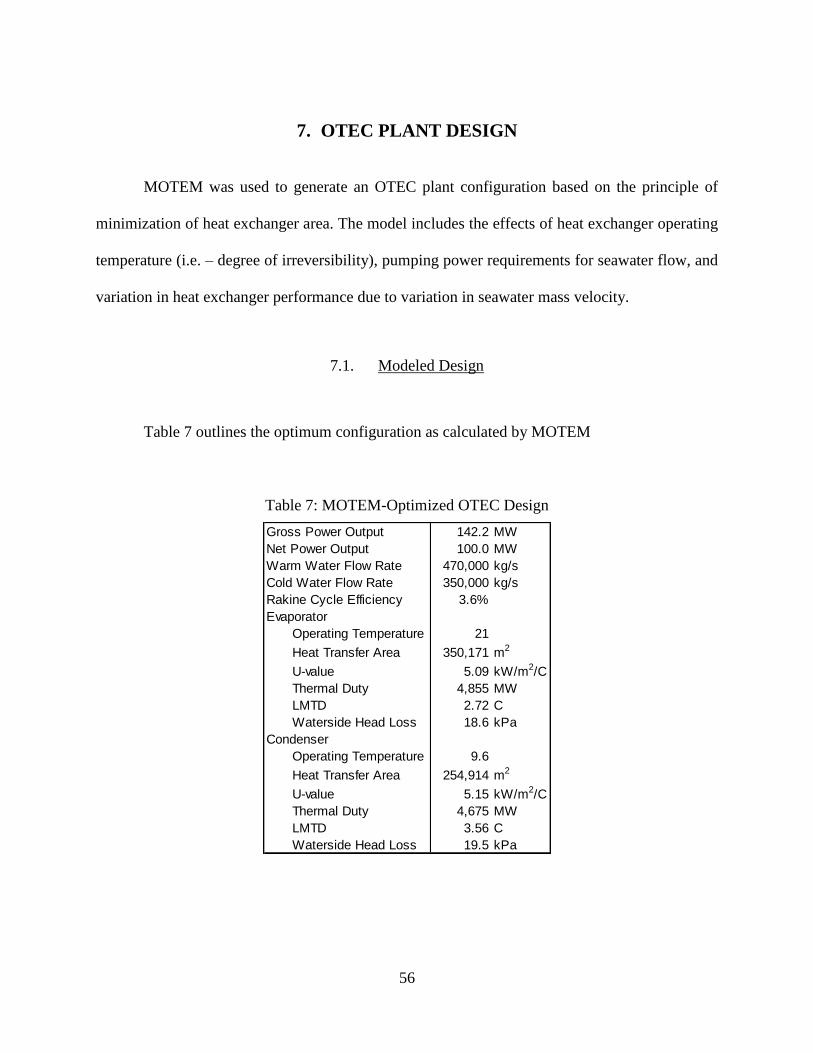
56

7. OTEC PLANT DESIGN

MOTEM was used to generate an OTEC plant configuration based on the principle of

minimization of heat exchanger area. The model includes the effects of heat exchanger operating

temperature (i.e. – degree of irreversibility), pumping power requirements for seawater flow, and

variation in heat exchanger performance due to variation in seawater mass velocity.

7.1. Modeled Design

Table 7 outlines the optimum configuration as calculated by MOTEM

Table 7: MOTEM-Optimized OTEC Design

Gross Power Output 142.2 MW

Net Power Output 100.0 MW

Warm Water Flow Rate 470,000 kg/s

Cold Water Flow Rate 350,000 kg/s

Rakine Cycle Efficiency 3.6%

Evaporator

Operating Temperature 21

Heat Transfer Area 350,171 m2

U-value 5.09 kW/m2/C

Thermal Duty 4,855 MW

LMTD 2.72 C

Waterside Head Loss 18.6 kPa

Condenser

Operating Temperature 9.6

Heat Transfer Area 254,914 m2

U-value 5.15 kW/m2/C

Thermal Duty 4,675 MW

LMTD 3.56 C

Waterside Head Loss 19.5 kPa

57

7.1.1. Thermal Efficiency

The thermal efficiency of the Rankine cycle is 3.6%. However, this value assumes

isentropic expansion in the turbine. Real turbines are not capable of true isentropic expansion.

Makai Ocean Engineering has approached turbine manufacturers for OTEC component

performance, and they have indicated that OTEC turbines can be expected to have a working-

fluid-to-electricity efficiency of 81%. This reduces the practical efficiency of the Rankine cycle

to 2.9%. Additionally, 42.2 MW of power is required to operate the plant, so only 100 MW of

power is available for export. Accounting for the parasitic power results in an overall plant

efficiency of 2%.

7.1.2. Ratio of Warm Water Flow to Cold Water Flow

The warm water flow rate is higher than the cold water flow rate, despite the fact that

both evaporators and condensers have identical performance characteristics. The difference

exists because of the practical effects of the cold water pipe. The OTEC heat sink and heat

source are not equally available; cold water must be drawn up a pipe, while warm water is

readily accessible. The cold water flow through a pipe reaching 1,000 m water depth is

associated with a non-trivial head loss. The head loss associated with drawing warm seawater

from the surface of the ocean is comparatively small. For any given flow rate, the higher head

loss in the cold water flow path requires more pumping power than does the lower head loss in

the warm water flow path.

58

Since all the power to run an OTEC plant must be generated by the plant itself, including

the power required for seawater pumping, cold seawater “costs” more than does warm seawater.

Previous work has shown that the benefits of reducing cold water flow with respect to warm

water flow outweigh the penalties, and that the optimum ratio of cold water flow to warm water

flow is expected to be 1.6:1 (Makai Ocean Engineering, 2005). The optimum warm water to cold

water ratio is unique to any given evaporator and condenser pair. The ratio of 1.34:1 seen in

Table 7 is likely an artifact of the artificial heat exchanger performance curves used in the

analysis.

7.1.3. Relative Performance of Evaporators and Condensers

The fact that the cold water flow rate is less than the warm water flow rate affects the

relative performance of the evaporators and condensers. In the absence of operating temperature

optimization, the reduced cold water flow rate would result in a reduced condenser heat transfer

coefficient. The reduced heat transfer coefficient would necessitate large condensers to

accommodate the required thermal duty. To compensate for this effect, the optimization process

increased the difference between the condenser operating temperature and the cold seawater

temperature (5.5o C) compared to that between the evaporator operating temperature and the

warm seawater temperature (4.7o C). This increases the LMTD of the condenser and allows for a

reduction in condenser heat transfer area. It also reduces the thermal efficiency of the plant,

which requires additional heat transfer area and slightly counteracts the gains from increased

condenser LMTD.

59

The overall effect of the optimization process is that evaporator performance and

condenser performance are similar. The reduced cold water flow rate is compensated by

increased LMTD and reduced area. See Section 6.1 for a discussion on the effects of increased

condenser LMTD.

7.2. Comparison to Isothermal Heat Reservoirs with a Carnot Engine

Wu’s method is not well suited to overall OTEC optimization since the heat transfer

coefficient and heat transfer areas of the heat exchangers must be known a priori. Therefore, the

values computed with MOTEM were used to calculate the predicted optimum operating

temperatures. However, MOTEM is based on a Rankine cycle and does not assume isothermal

heat reservoirs. As a result, the operating temperatures predicted by equations (5) and (6) do not

produce a viable system in conjunction with the MOTEM-selected seawater flow rates; the

calculated condenser duty is insufficient to maintain the specified condenser temperature.

To compensate for the problem, the MOTEM seawater flow rates were adjusted such that

the OTEC system was viable. The seawater flows were then reoptimized to ensure the best

possible values were selected. The reoptimization resulted in a change in the heat transfer

coefficients and heat transfer areas of the evaporator and condenser. The new values were used

to compute new predicted optimum operating temperatures. Multiple iterations between

MOTEM and equations (5) through (7) were carried out.

60

7.2.1. Comparison with Artificial Heat Exchanger Performance Curves

With a warm water surface temperature of 25.7o C and a cold deep temperature of 4.1

o C,

equations (5) and (6) predict that the optimum evaporator operating temperature is 20.6o C and

the optimum condenser operating temperature is 9.8o C. Predicted efficiency is 3.68%.

The relative efficiency of the predicted optimum operating temperatures was evaluated

by entering them into MOTEM and comparing the results with the MOTEM-optimized system.

MOTEM predicts that a system designed to operate at 20.6o C and 9.8

o C will produce 99 MW of

electrical power, a 1% reduction from the MOTEM-optimized case. The thermal efficiency of

the power cycle is 3.42%, 7% lower than predicted by equation (8).

7.2.2. Comparison with Real World Heat Exchanger Curves

As an additional test, Wu’s predicted operating temperatures were fed into a version of

MOTEM using real-world heat exchanger performance data provided by Makai Ocean

Engineering. The performance details are proprietary, but the shape and magnitude of the

performance curves generally agree with those from equations (25) through (27). The condenser

heat transfer coefficient curve is similar to the evaporator heat transfer coefficient curve, but the

seawater head loss curve is 4-5 times higher.


o C,

equations (5) and (6) predict that the optimum evaporator operating temperature is still 20.6o C

and the optimum condenser operating temperature is still 9.8o C. Predicted efficiency remains

unchanged at 3.68%. MOTEM predicts that a system designed to operate at 20.6o C and 9.8

o C

61

will produce 97 MW of electrical power using real world heat exchangers, which represents a

3% reduction from the MOTEM-optimized case. The thermal efficiency of the power cycle is

3.42%, 7% lower than predicted by equation (8).

7.3. Comparison to Heat Reservoirs with Varying Properties and a Rankine Engine

Khaliq’s optimization algorithm is not dependent on heat exchanger area or heat transfer

coefficient, only the seawater temperatures. Thus, no iteration process was required to evaluate

the relative efficiency of an OTEC plant designed according to equations (9) and (10).

7.3.1. Comparison with Artificial Heat Exchanger Performance Curves


o C,

equations (9) and (10) predict an optimum evaporator operating temperature of 20.2o C and an

optimum condenser operating temperature of 9.4o C. Predicted efficiency is 3.68%.


by entering them into MOTEM and comparing the results with the MOTEM-optimized system.

MOTEM predicts that a system designed to operate at 20.2o C and 9.4

o C will produce 97 MW of

electrical power, a 3% reduction from the MOTEM-optimized case. The thermal efficiency of

the power cycle is 3.42%, 7% lower than predicted by equation (8).

62

7.3.2. Comparison with Real World Heat Exchanger Curves

Since heat exchanger performance does not influence Khaliq’s algorithm, the predicted

optimum evaporator operating temperature remains at 20.2o C and the optimum predicted

condenser operating temperature remains at 9.4o C. Predicted efficiency is still 3.68%.


by entering them into MOTEM, with real world heat exchanger performance data, and

comparing the results with the MOTEM-optimized system. MOTEM predicts that a system

designed to operate at 20.2o C and 9.4

o C will produce 93 MW of electrical power, a 7%

reduction from the MOTEM-optimized case. The thermal efficiency of the power cycle is 3.43%,

7% lower than predicted by equation (8).

7.4. Summary of Comparison Results

Table 8 and Table 9 compare the optimum heat exchanger operating temperatures

predicted by Wu and Khaliq with those predicted by MOTEM.

63

Table 8: Optimum Heat Exchanger Operating Temperatures with Artificial Heat Exchangers

The amount of net power predicted by MOTEM is the maximum amount of power

possible with the available heat transfer area. Both Wu’s method and Khaliq’s method produce

less power when using the artificial heat exchanger performance curves, though Wu’s method is

in better agreement with MOTEM than is Khaliq’s method. Both published methods apportion

more temperature difference to heat transfer than MOTEM. MOTEM and Wu’s method reserve

significantly more temperature difference for condensation than for evaporation.

Table 9: Optimum Heat Exchanger Operating Temperatures with Real World Heat Exchangers

MOTEM Wu Khaliq

Net Power Output 100 99 97 MW

Thermodynamic Cycle Efficiency 3.61% 3.42% 3.42%

Heat Transfer Coefficient Ratio 0.99 0.95 0.85

Evaporator Operating Temperature 21.0 20.6 20.2 C

Condenser Operating Temperature 9.6 9.8 9.4 C

Total Temperature Difference Available 21.6 21.6 21.6 C

Difference Available for Rankine Cycle 11.4 10.8 10.8 C

Difference Available for Heat Transfer 10.2 10.8 10.8 C

Difference Reserved for Evaporation 4.7 5.1 5.5 C

Difference Reserved for Condensation 5.5 5.7 5.3 C

MOTEM Wu Khaliq

Net Power Output 100 97 93 MW

Thermodynamic Cycle Efficiency 3.52% 3.42% 3.43%

Heat Transfer Coefficient Ratio 1.45 1.27 1.14

Evaporator Operating Temperature 21.2 20.6 20.2 C

Condenser Operating Temperature 10.1 9.8 9.4 C

Total Temperature Difference Available 21.6 21.6 21.6 C

Difference Available for Rankine Cycle 11.1 10.8 10.8 C

Difference Available for Heat Transfer 10.5 10.8 10.8 C

Difference Reserved for Evaporation 4.5 5.1 5.5 C

Difference Reserved for Condensation 6.0 5.7 5.3 C

64

The predicted optimum conditions calculated by Wu’s method and Khaliq’s method are

unchanged due the switch to real world heat exchanger performance. MOTEM’s results reserve

more temperature difference for heat transfer and devote proportionally more temperature

difference to condensation compared to the results with the artificial heat exchanger performance

curves. Both Wu’s method and Khaliq’s method produce less power with real world heat

exchangers than they did with the artificial heat exchanger performance curves.

65

8. DISCUSSION

8.1. Temperature Optimization

Initial investigation of temperature optimization suggests it is critical to successful OTEC

plant design. Figure 7 and Figure 8 show that heat transfer area requirements can increase up to

45% when the operating temperature deviate from the optimum by 1.5o C. The importance of

temperature optimization is tied to the LMTD between the working fluid and seawater under

optimum conditions. Heat transfer area is more sensitive to changes in evaporator operating

temperature because the evaporator LMTD is lower than that of the condenser. Similarly, a

deviation from the optimum value that decreases LMTD is more detrimental than a deviation that

increases LMTD.

8.2. Water Flow Optimization

Total heat transfer area is slightly more sensitive to cold water optimization than to warm

water optimization, particularly when the flow rate is decreased. Figure 12 and Figure 13 show

that a 20% increase in flow relative to the optimum value causes a 6% increase in heat transfer

area for warm water and an 8% increase for cold water. If flow rates are decreased, the heat

transfer area deviation grows to 9% for warm water and 15% for cold water. The reason for the

asymmetry is two-fold.

Firstly, decreasing the flow rate will increase the seawater temperature change through

the heat exchanger and decrease LMTD. A decrease in LMTD is more detrimental than an

increase in LMTD. For any given magnitude of deviation, a decrease represents a proportionally

66

larger amount than does an increase. Therefore, optimization curves are asymmetrical in that

increasing seawater flow rate causes less of an impact than decreasing seawater flow rate.

Secondly, the magnification effects discussed in Sections 3.1 and 3.2 favor increases in

seawater flow rate. When the flow rate is increased, the head loss and parasitic pumping power

requirements increase, but so does heat transfer coefficient. The increased heat transfer

coefficient helps to counteract the increase in area required to compensate for the added parasitic

power. Conversely, a decrease in flow rate reduces pumping power requirements, but also

reduces heat transfer coefficient. The reduced heat transfer coefficient counteracts the area

reduction permitted by the reduced pumping power.

The effects of heat transfer coefficient reduction and pumping power reduction are

competing. The shapes of Figure 12 and Figure 13 indicate that the heat transfer coefficient

effect is dominant. This conclusion may be tied to the specific heat exchanger performance

curves used. If heat transfer coefficient is insensitive to seawater flow, but head loss is very

sensitive, then asymmetry in the figures will likely be reversed, and increases in seawater flow

rate will be more detrimental than decreases.

8.3. Combined Optimization

The ability to optimize both operating temperatures and seawater flow rates significantly

mitigates the effects of sub-optimum selection of a single design parameter. Figure 9 and Figure

10 show that optimization of seawater flow rate reduces the penalty for suboptimum heat

exchanger operating condition selection by a factor of 4. A similar effect is seen in Figure 12 and

67

Figure 13; optimization of operating temperatures reduces the penalty for suboptimum water

flows by a factor of 4.

In Figure 11, both evaporator and condenser operating temperatures are varied. The

variation is symmetric, such that a positive variation is defined as an increase in evaporator

operating temperature and a decrease in condenser operating temperature. The results contradict

the pattern discussed above in that seawater flow optimization has a negligible effect on the

penalties associated with suboptimum heat exchanger operating temperature selection. This

suggests that sets of heat exchanger operating temperatures exist for which the optimum

seawater flow rates are identical. Furthermore, it suggests that there is a relationship governing

the set that includes the optimum configuration. Review of the ratio of evaporator heat transfer

coefficient to condenser heat transfer coefficient along an optimization curve revealed that all

configurations in which optimum seawater flows are selected share a common ratio. Section 8.6

explores the implications behind the common heat transfer coefficient ratio.

8.4. Heat Exchanger Performance

A 25% increase in the artificial heat transfer coefficient curve results in a 29%-30%

increase in heat transfer coefficient in the optimum configuration. The effective increase is larger

than the performance curve scale factor due to the magnification effect discussed in Section 3.1.

The magnification effect is counteracted by the seawater flow rate optimization process. As the

overall heat transfer coefficient increases and heat transfer area decreases, seawater pressure

drop increases. An increase in seawater pressure drop reduces the penalty of reducing seawater

flow at the expense of heat transfer coefficient, and the optimum seawater flow rate shifts

68

downwards. Table 6 illustrates this effect in that the optimum seawater flow when heat transfer

coefficient is increased is 9% lower than in the baseline design.

A 50% decrease in the artificial seawater pressure drop curve results in a 24%-25%

decrease in the seawater pressure drop in the optimum configuration. A magnification effect is

also responsible for the mitigation of the change in pressure drop. As seawater pressure drop

decreases, the parasitic power requirement of the plant decreases, and therefore gross power

decreases. The decrease in gross power means that less thermal duty is required. The reduction in

thermal duty allows for a reduction in heat transfer area. The reduction in heat transfer area

increases the seawater mass velocity, which increases the seawater pressure drop. The increase in

seawater pressure drop counteracts the 50% reduction applied to the performance curve. The

magnification effect is exacerbated by the seawater optimization process. A reduction in

seawater pressure reduces the penalty associated with increasing seawater flow rate to enhance

heat transfer coefficient, so the optimum seawater flow rates will shift upwards. Table 6

illustrates this effect in that the optimum seawater flow when seawater pressure drop is reduced

is 6% higher than in the baseline design.

8.5. Comparison between MOTEM Results and Results in the Literature

The total temperature difference available between warm and cold seawater is 21.6o C.

Of that, MOTEM predicts that 11.4o C should be devoted to power generation and 10.2

o C

should be devoted to driving heat transfer when artificial heat exchanger performance curves are

used. When using real world heat exchangers, MOTEM predicts that 11.1o C should be devoted

to power generation and 10.5o C to heat transfer. Both Wu’s and Khaliq’s methods predict that

69

10.8o C should be reserved for power generation regardless of the selected heat exchanger

performance curves. A discrepancy exists among the three methods when considering how the

temperature differential reserved for heat transfer should be apportioned.

When considering artificial heat exchangers, all three methods are in general agreement.

MOTEM and Wu’s method both recommend more temperature difference for the condenser than

for the evaporator. As discussed in Section 7.1.3, an optimum OTEC plant is expected to use

more cold seawater than warm seawater. Reserving more temperature difference for the

condenser than the evaporator compensates for the relative reduction in cold water flow and

keeps condenser heat transfer area low. The influence of cold seawater flow rate was introduced

to Wu’s during the iterative calculations with MOTEM. Khaliq’s method did not require

iteration, and reserves a similar amount of temperature difference for both evaporators and

condensers.

When considering real world heat exchangers, MOTEM is not in agreement with

predictions from Wu and Khaliq. Neither Wu’s nor Khaliq’s recommended operating

temperatures change, but MOTEM’s recommendation changes significantly. The seawater head

loss curve for the real world condenser is 4-5 times higher than that for the evaporator. This

drives the optimization in favor of low condenser mass velocity, and therefore low overall heat

transfer coefficient. MOTEM recommends reserving additional temperature difference for the

condenser, even at the expense of temperature difference available to the Rankine cycle.

Despite differences in predicted optimum heat exchanger operating temperatures,

MOTEM and Wu’s method produce comparably optimized OTEC plants. If Wu’s predicted

temperatures are used to design an OTEC plant using the artificial heat exchanger performance

curves, the net power output is 99% of the maximum possible plant output. If real world heat

70

exchanger performance curves are used, the net power output of that a plant designed with Wu’s

method would be 97% of the maximum possible plant output. In spite of the fact that it uses a

Rankine cycle and relaxes the assumption that the OTEC heat source and sink are isothermal,

Khaliq’s method does not perform as well. A design using recommended operating temperatures

calculated from equations (9) and (10) would produce 3% less than a fully optimized plant if

artificial heat exchanger performance curves are used, and 7% less if real world heat exchangers

are used.

The deficiency in Khaliq’s algorithm likely lies with the implicit assumption that heat

transfer coefficient is insensitive to changes in seawater mass velocity through the heat

exchanger (see Section 2.2.1). This paper has shown that OTEC optimization is sensitive to heat

exchanger performance, and Khaliq’s algorithm excludes heat exchanger performance effects

from the calculations by allowing seawater flow rate to vary independently of heat transfer

coefficient. Wu’s method provides a better estimate of optimum heat exchanger operating

temperatures because a set of heat exchanger performance curves can be used to adapt it to

compensate for the fixed seawater flow rate (as discussed in Section 7.2).

8.6. Heat Transfer Coefficient Ratio

Table 4 and Table 5 show there is a correlation between the potential for heat transfer

area reduction via further optimization and the ratio between evaporator overall heat transfer

coefficient and condenser overall heat transfer coefficient. If any particular pair of evaporator

and condenser operating temperatures has the same heat transfer coefficient ratio as is found in

the optimized configuration, no further optimization via variation in seawater flow rate is

71

possible. The best possible configuration has been achieved for that particular operating

temperature pair. Table 8 and Table 9 reinforce the correlation between heat transfer coefficient

and OTEC plant optimization. Wu’s method, which produces more net power and is therefore

closer to an optimum design, results in a heat transfer coefficient ratio closer to that calculated by

MOTEM than does Khaliq’s method.

The fact that the artificial heat exchangers and real world heat exchangers have different

optimum heat transfer coefficient ratios indicates that the ratio is a function of heat exchanger

performance curves. The fact that the optimum heat transfer coefficient ratio for the artificial

heat exchangers is 1 suggests that it is related to the ratio of the performance of the evaporator

and the condenser. Therefore, the optimum ratio will be specific to each combination of

evaporator and condenser, and is therefore a characteristic feature of the heat exchanger pair.

Further research into the relationship between heat transfer coefficient ratio and heat exchanger

performance is recommended.

8.6.1. Direct Calculation of Heat Transfer Coefficient Ratio

If a correlation can be drawn between heat exchanger performance curves and the

optimum heat transfer coefficient ratio, then OTEC optimization will become easier. Ideally, the

relationship could be combined with existing published finite-time thermodynamic OTEC

optimization algorithms to compute optimum operating conditions without the need for the

simulation capabilities in MOTEM. This would allow the suitability of competing heat

exchanger concepts to be evaluated quickly, and would speed up development of OTEC-specific

designs.

72

Since real world heat exchangers exhibit a range of functional forms in their performance

correlations, a numerical solution will likely be required for practical applications. Further

research into the relationship between optimum heat transfer coefficient ratio and heat exchanger

performance curves is recommended.

8.6.2. Improvements to MOTEM

Even if no direct correlation between heat transfer coefficient ratio and heat exchanger

performance can be determined, MOTEM could be improved to take advantage of the results of

this research. In the current algorithm, MOTEM separately searches the entire solution spaces for

both heat exchanger operating temperature and seawater flow rate. It alternates between the two

parameter pairs until a stable configuration is reached. However, optimization of either pair of

parameters will provide the correct heat transfer coefficient ratio for the fully optimized plant.

Once the optimum ratio is known, the solution space on subsequent iterations can be reduced to

those values that share the same ratio.

The reduction in solution space, if large enough, could eliminate the need for alternation

between operating temperature and seawater flow rate optimization. If the relationship between

seawater flow rate and heat transfer coefficient were pre-calculated, then a set of allowable warm

and cold seawater flow rate pairs could be determined for any given pair of operating conditions.

The allowable pairs represent a linear space rather than the original quadratic space. The size of

the total solution space would be reduced by a factor of n, where n is the number of allowable

values; it would be reduced from n4 to n

3. Such a reduction could avoid the need to split the

solution space into two segments and improve the accuracy of the optimization process.

73

9. CONCLUSIONS

The optimum heat exchanger operating temperatures and seawater flow rates predicted

by MOTEM vary when the heat exchanger performance curves are altered. Therefore, OTEC

optimization is sensitive to heat exchanger performance. Deviation from the optimum parameters

results in a reduction in net power output for any given configuration. Previously published

finite-time thermodynamic optimization algorithms do not include the effects of heat exchanger

performance curves. As a result, they make sub-optimum recommendations of heat exchanger

operating temperatures and no recommendations regarding seawater flow rate. Of the published

optimization algorithms tested, Wu’s method performed the best with a maximum deviation of

3% from optimum power output when real world heat exchanger data is used. Wu’s method also

performs best, with a 1% deviation from optimum power output, when evaporator and condenser

performance is identical. It can be concluded that the magnitude of the deviation between the

optimum configuration and the configuration recommended by finite-time thermodynamic

optimization is related to the difference between evaporator and condenser performance.

Warm seawater from the surface of the ocean and cold deep seawater from 1,000 m water

depth have different costs associated with them. Cold seawater must be pumped up a long pipe,

whereas warm seawater is readily available, which results in a higher proportion of the parasitic

power being devoted to cold water pumping than warm water pumping. The fact that the OTEC

plant must produce extra power to pump the cold seawater causes MOTEM to predict a higher

warm water flow rate than cold water flow rate at optimum conditions. Finite-time

thermodynamic optimization algorithms do not include the effects of seawater pumping, and

therefore do not include the effects of asymmetric seawater flow rates.

74

The ratio of evaporator and condenser overall heat transfer coefficients is a good metric

for the relative optimization of a particular OTEC configuration. Any configuration in which the

seawater flow rate is ideal for the selected heat exchanger operating temperatures shares the

same heat transfer coefficient ratio with the overall optimum configuration. Unfortunately, no

method currently exists to determine the optimum value a priori. Therefore, the heat transfer

coefficient ratio is currently only effective at evaluating sub-optimum configurations relative to a

known optimum configuration. If a solution for the ideal heat transfer coefficient were found, it

would allow rapid relative evaluation of evaporator condenser pairs and could speed up the

optimization algorithm in MOTEM.

75

10. FUTURE WORK

10.1. Model Validation

The conclusions presented in this paper are dependent on the accuracy of MOTEM.

While the fact that MOTEM is programmed as a simulator means that verification with basic test

cases has already been carried out, no validation against a real OTEC system has been possible

because no suitable system currently exists. Once an OTEC test system is constructed,

MOTEM’s alternate mode can be used for validation. In alternate mode, the heat exchanger area

is fixed and MOTEM predicts the amount of power that will be produced. If the power output of

a test facility and that predicted by MOTEM match, then overall calculations of the model will

have been validated. Full validation will require that the test facility be fully instrumented so

each of MOTEM’s calculation steps can be checked.

10.2. Investigation of Heat Transfer Coefficient Ratio

The ratio of evaporator and condenser overall heat transfer coefficients has been found to

be characteristic of the level of optimization of an OTEC plant. The ratio is constant over a wide

range of heat exchanger operating temperatures provided that optimum seawater flow rates have

been selected. The existence of a characteristic ratio implies that the ideal ratio should be

calculable from the heat exchanger performance curves. Additional work is recommended to

investigate the relationship between the shape of heat exchanger performance curves and the heat

transfer coefficient ratio. If a relationship is discovered, then MOTEM should be improved to

take advantage of it in order to reduce the size of the solution space and speed up optimization.

76

10.3. OTEC Cost Estimation

Minimization of heat exchanger area is a useful approximation for minimization of

OTEC plant capital cost, but true optimization on cost would be superior. Refinement of OTEC

costs will be dependent upon development of a pilot plant producing at least 10 MW of net

electrical power output. If and when such a plant is constructed, the cost details should be

entered into MOTEM’s cost estimation module, and the analysis presented in this paper should

be confirmed.

77

11. REFERENCES

Avery, W., & Wu, C. (1994). Renewable energy from the ocean. (pp. 90-201). New York, NY:

Oxford University Press.

Chen, L., Sun, F., & Wu, C. (1997). Influence of heat transfer low on the performance of a

Carnot engine. Applied Thermal Engineering, 17(3), 277-282.

Curzon, F. & Ahlborn, B. (1975). Efficiency of a Carnot engine at maximum power output.

American Journal of Physics, 43, 22-24.

Kazim, A. (2005). Hydrogen production through an ocean thermal energy conversion system

operating at an optimum temperature drop. Applied Thermal Engineering, 25, 2236-2246.

Khaliq, A. (2004). Finite-time heat-transfer analysis and generalized power-optimization of an

endoreversible Rankine heat-engine. Applied Energy, 79, 27-40.

Lee, W., & Kim, S. (1990). Finite-time optimizations of a heat engine. Energy, 15(11), 979-985.

Lee, W., & Kim, S. (1991). Finite-time optimizations of an irreversible heat engine. Energy,

16(7), 1051-1058.

Makai Ocean Engineering. United States Department of the Navy, Office of Naval Research.

(2005). Integration and optimization of hydrogen production with ocean thermal energy

conversion technology in offshore floating platforms.

Press, W., Flannery, B., Teukolsky, S., & Vetterling, W. (1997). Numerical recipes in C, the art

of scientific computing. (2 ed., pp. 294-444). Cambridge, England: Cambridge University

Press.

Sahin, B., & Kodal, A. (2001). Performance analysis of an endoreversible heat engine based on a

new thermoeconomic optimization criterion. Energy Conversion and Management, 42,

1085-1093.

Sahin, B., Kodal, A., & Yavuz, H. (1996). Maximum power density for an endoreversible Carnot

heat engine. Energy, 21(12), 1219-1225.

Sun, F., Ikegami, Y., & Arima, H. (2012). Optimization design and exergy analysis of organic

Rankine cycle in ocean thermal energy conversion. Applied Ocean Research, 35, 38-46.

Wu, C. (1987). A performance bound for real OTEC heat engines. Ocean Engineering, 14(4),

349-354.

78

Wu, C. (1989). Power optimization of a finite-time Rankine heat engine. International Journal of

heat and Fluid Flow, 10(2), 134-138.

Wu, C. (1990). Specific power optimization of closed-cycle OTEC plants. Ocean Engineering,

17(3), 307-314.

Wu, C. (1991). Specific power bound of real heat engines. Energy Conversion and Management,

32(3), 249-253.

Wu, C. (1993). Specific power analysis of thermoelectric OTEC plants. Ocean Engineering,

20(4), 433-442.

Yilmaz, T., Ust, Y., & Erdil, A. (2006). Optimum operating conditions of irreversible solar

driven heat engines. Renewable Energy, 31, 1333-1342.

Documents

Optimization Of Ocean Thermal Energy Conversion Power Plants