Embed Size (px)
Citation preview

Optimization-Based Control
Richard M. Murray
Control and Dynamical Systems
California Institute of Technology
DRAFT v2.1a, January 4, 2010c© California Institute of Technology
All rights reserved.
This manuscript is for review purposes only and may not be reproduced, in whole or inpart, without written consent from the author.

Chapter 2
Optimal Control
This set of notes expands on Chapter 6 of Feedback Systems by Astrom and Murray(AM08), which introduces the concepts of reachability and state feedback. We alsoexpand on topics in Section 7.5 of AM08 in the area of feedforward compensation.Beginning with a review of optimization, we introduce the notion of Lagrange mul-tipliers and provide a summary of the Pontryagin’s maximum principle. Using thesetools we derive the linear quadratic regulator for linear systems and describe itsusage.
Prerequisites. Readers should be familiar with modeling of input/output controlsystems using differential equations, linearization of a system around an equilib-rium point and state space control of linear systems, including reachability andeigenvalue assignment. Some familiarity with optimization of nonlinear functions isalso assumed.
2.1 Review: Optimization
Optimization refers to the problem of choosing a set of parameters that maximizeor minimize a given function. In control systems, we are often faced with having tochoose a set of parameters for a control law so that the some performance conditionis satisfied. In this chapter we will seek to optimize a given specification, choosingthe parameters that maximize the performance (or minimize the cost). In thissection we review the conditions for optimization of a static function , and thenextend this to optimization of trajectories and control laws in the remainder ofthe chapter. More information on basic techniques in optimization can be foundin [Lue97] or the introductory chapter of [LS95].
Consider first the problem of finding the minimum of a smooth function F :R
n → R. That is, we wish to find a point x∗ ∈ Rn such that F (x∗) ≤ F (x) for all
x ∈ Rn. A necessary condition for x∗ to be a minimum is that the gradient of the
function be zero at x∗:∂F
∂x(x∗) = 0.
The function F (x) is often called a cost function and x∗ is the optimal value for x.Figure 2.1 gives a graphical interpretation of the necessary condition for a minimum.Note that these are not sufficient conditions; the points x1 and x2 and x∗ in thefigure all satisfy the necessary condition but only one is the (global) minimum.
The situation is more complicated if constraints are present. Let Gi : Rn →
R, i = 1, . . . , k be a set of smooth functions with Gi(x) = 0 representing theconstraints. Suppose that we wish to find x∗ ∈ R
n such that Gi(x∗) = 0 and
F (x∗) ≤ F (x) for all x ∈ x ∈ Rn : Gi(x) = 0, i = 1, . . . , k. This situation can be

2.1. REVIEW: OPTIMIZATION 2-2
dx
x∗
x1
x2
x
F (x)
∂F
∂xdx
Figure 2.1: Optimization of functions. The minimum of a function occurs at apoint where the gradient is zero.
x1
x∗
F (x)
G(x) = 0
x2
(a) Constrained optimization
x2
G(x) = 0
∂G
∂x x3
x1
(b) Constraint normalvectors
Figure 2.2: Optimization with constraints. (a) We seek a point x∗ that minimizesF (x) while lying on the surface G(x) = 0 (a line in the x1x2 plane). (b) We canparameterize the constrained directions by computing the gradient of the constraintG. Note that x ∈ R
2 in (a), with the third dimension showing F (x), while x ∈ R3
in (b).
visualized as constraining the point to a surface (defined by the constraints) andsearching for the minimum of the cost function along this surface, as illustrated inFigure 2.2a.
A necessary condition for being at a minimum is that there are no directionstangent to the constraints that also decrease the cost. Given a constraint functionG(x) = (G1(x), . . . , Gk(x)), x ∈ R
n we can represent the constraint as a n − kdimensional surface in R
n, as shown in Figure 2.2b. The tangent directions to thesurface can be computed by considering small perturbations of the constraint thatremain on the surface:
Gi(x+ δx) ≈ Gi(x) +∂Gi
∂x(x)δx = 0. =⇒ ∂Gi
∂x(x)δx = 0,
where δx ∈ Rn is a vanishingly small perturbation. It follows that the normal
directions to the surface are spanned by ∂Gi/∂x, since these are precisely the vectorsthat annihilate an admissible tangent vector δx.
Using this characterization of the tangent and normal vectors to the constraint, anecessary condition for optimization is that the gradient of F is spanned by vectors

2.1. REVIEW: OPTIMIZATION 2-3
that are normal to the constraints, so that the only directions that increase thecost violate the constraints. We thus require that there exist scalars λi, i = 1, . . . , ksuch that
∂F
∂x(x∗) +
k∑
i=1
λi
∂Gi
∂x(x∗) = 0.
If we let G =[G1 G2 . . . Gk
]T, then we can write this condition as
∂F
∂x+ λT ∂G
∂x= 0 (2.1)
the term ∂F/∂x is the usual (gradient) optimality condition while the term ∂G/∂xis used to “cancel” the gradient in the directions normal to the constraint.
An alternative condition can be derived by modifying the cost function to incor-porate the constraints. Defining F = F +
∑λiGi, the necessary condition becomes
∂F
∂x(x∗) = 0.
The scalars λi are called Lagrange multipliers. Minimizing F is equivalent to theoptimization given by
minx
(F (x) + λTG(x)
). (2.2)
The variables λ can be regarded as free variables, which implies that we need tochoose x such that G(x) = 0 in order to insure the cost is minimized. Otherwise,we could choose λ to generate a large cost.
Example 2.1 Two free variables with a constraint
Consider the cost function given by
F (x) = F0 + (x1 − a)2 + (x2 − b)2,
which has an unconstrained minimum at x = (a, b). Suppose that we add a con-straint G(x) = 0 given by
G(x) = x1 − x2.
With this constraint, we seek to optimize F subject to x1 = x2. Although in thiscase we could do this by simple substitution, we instead carry out the more generalprocedure using Lagrange multipliers.
The augmented cost function is given by
F (x) = F0 + (x1 − a)2 + (x2 − b)2 + λ(x1 − x2),
where λ is the Lagrange multiplier for the constraint. Taking the derivative of F ,we have
∂F
∂x=
[2x1 − 2a+ λ 2x2 − 2b− λ
].
Setting each of these equations equal to zero, we have that at the minimum
x∗1 = a− λ/2, x∗2 = b+ λ/2.

2.2. OPTIMAL CONTROL OF SYSTEMS 2-4
The remaining equation that we need is the constraint, which requires that x∗1 = x∗2.Using these three equations, we see that λ∗ = a− b and we have
x∗1 =a+ b
2, x∗2 =
a+ b
2.
To verify the geometric view described above, note that the gradients of F andG are given by
∂F
∂x=
[2x1 − 2a 2x2 − 2b
],
∂G
∂x=
[1 −1
].
At the optimal value of the (constrained) optimization, we have
∂F
∂x=
[b− a a− b
],
∂G
∂x=
[1 −1
].
Although the derivative of F is not zero, it is pointed in a direction that is normalto the constraint, and hence we cannot decrease the cost while staying on theconstraint surface. ∇
We have focused on finding the minimum of a function. We can switch back andforth between maximum and minimum by simply negating the cost function:
maxx
F (x) = minx
(−F (x)
)
We see that the conditions that we have derived are independent of the sign of Fsince they only depend on the gradient begin zero in approximate directions. Thusfinding x∗ that satisfies the conditions corresponds to finding an extremum for thefunction.
Very good software is available for solving optimization problems numerically ofthis sort. The NPSOL and SNOPT libraries are available in FORTRAN (and C).In MATLAB, the fmin function can be used to solve a constrained optimizationproblem.
2.2 Optimal Control of Systems
Consider now the optimal control problem:
minu(·)
∫ T
0
L(x, u) dt+ V(x(T )
)
subject to the constraint
x = f(x, u), x ∈ Rn, u ∈ R
m.
Abstractly, this is a constrained optimization problem where we seek a feasibletrajectory (x(t), u(t)) that minimizes the cost function
J(x, u) =
∫ T
0
L(x, u) dt+ V(x(T )
).

2.2. OPTIMAL CONTROL OF SYSTEMS 2-5
More formally, this problem is equivalent to the “standard” problem of minimizing acost function J(x, u) where (x, u) ∈ L2[0, T ] (the set of square integrable functions)and h(z) = x(t) − f(x(t), u(t)) = 0 models the dynamics. The term L(x, u) isreferred to as the integral cost and V (x(T )) is the final (or terminal) cost.
There are many variations and special cases of the optimal control problem. Wemention a few here:
Infinite horizon optimal control. If we let T = ∞ and set V = 0, then we seek tooptimize a cost function over all time. This is called the infinite horizon optimalcontrol problem, versus the finite horizon problem with T < ∞. Note that if aninfinite horizon problem has a solution with finite cost, then the integral cost termL(x, u) must approach zero as t→ ∞.
Linear quadratic (LQ) optimal control. If the dynamical system is linear and thecost function is quadratic, we obtain the linear quadratic optimal control problem:
x = Ax+Bu, J =
∫ T
0
(xTQx+ uTRu
)dt+ xT (T )P1x(T ).
In this formulation, Q ≥ 0 penalizes state error, R > 0 penalizes the input andP1 > 0 penalizes terminal state. This problem can be modified to track a desiredtrajectory (xd, ud) by rewriting the cost function in terms of (x−xd) and (u−ud).
Terminal constraints. It is often convenient to ask that the final value of the tra-jectory, denoted xf , be specified. We can do this by requiring that x(T ) = xf or byusing a more general form of constraint:
ψi(x(T )) = 0, i = 1, . . . , q.
The fully constrained case is obtained by setting q = n and defining ψi(x(T )) =xi(T )− xi,f . For a control problem with a full set of terminal constraints, V (x(T ))can be omitted (since its value is fixed).
Time optimal control. If we constrain the terminal condition to x(T ) = xf , let theterminal time T be free (so that we can optimize over it) and choose L(x, u) = 1,we can find the time-optimal trajectory between an initial and final condition. Thisproblem is usually only well-posed if we additionally constrain the inputs u to bebounded.
A very general set of conditions are available for the optimal control problem thatcaptures most of these special cases in a unifying framework. Consider a nonlinearsystem
x = f(x, u), x = Rn,
x(0) given, u ∈ Ω ⊂ Rm,
where f(x, u) = (f1(x, u), . . . fn(x, u)) : Rn × R
m → Rn. We wish to minimize a
cost function J with terminal constraints:
J =
∫ T
0
L(x, u) dt+ V (x(T )), ψ(x(T )) = 0.
The function ψ : Rn → R
q gives a set of q terminal constraints. Analogous to thecase of optimizing a function subject to constraints, we construct the Hamiltonian:
H = L+ λT f = L+∑
λifi.

2.2. OPTIMAL CONTROL OF SYSTEMS 2-6
The variables λ are functions of time and are often referred to as the costate vari-ables. A set of necessary conditions for a solution to be optimal was derived byPontryagin [PBGM62].
Theorem 2.1 (Maximum Principle). If (x∗, u∗) is optimal, then there exists λ∗(t) ∈R
n and ν∗ ∈ Rq such that
xi =∂H
∂λi
− λi =∂H
∂xi
x(0) given, ψ(x(T )) = 0
λ(T ) =∂V
∂x(x(T )) + νT ∂ψ
∂x
andH(x∗(t), u∗(t), λ∗(t)) ≤ H(x∗(t), u, λ∗(t)) for all u ∈ Ω
The form of the optimal solution is given by the solution of a differential equationwith boundary conditions. If u = arg minH(x, u, λ) exists, we can use this to choosethe control law u and solve for the resulting feasible trajectory that minimizes thecost. The boundary conditions are given by the n initial states x(0), the q terminalconstraints on the state ψ(x(T )) = 0 and the n − q final values for the Lagrangemultipliers
λ(T ) =∂V
∂x(x(T )) + νT ∂ψ
∂x.
In this last equation, ν is a free variable and so there are n equations in n+ q freevariables, leaving n − q constraints on λ(T ). In total, we thus have 2n boundaryvalues.
The maximum principle is a very general (and elegant) theorem. It allows thedynamics to be nonlinear and the input to be constrained to lie in a set Ω, allowingthe possibility of bounded inputs. If Ω = R
m (unconstrained input) and H isdifferentiable, then a necessary condition for the optimal input is
∂H
∂u= 0.
We note that even though we are minimizing the cost, this is still usually called themaximum principle (an artifact of history).
Sketch of proof. We follow the proof given by Lewis and Syrmos [LS95], omittingsome of the details required for a fully rigorous proof. We use the method of La-grange multipliers, augmenting our cost function by the dynamical constraints andthe terminal constraints:
J(x(·), u(·), λ(·), ν) = J(x, u) +
∫ T
0
−λT (t)(x(t) − f(x, u)
)dt+ νTψ(x(T ))
=
∫ T
0
(L(x, u) − λT (t)
(x(t) − f(x, u)
)dt
+ V (x(T )) + νTψ(x(T )).
Note that λ is a function of time, with each λ(t) corresponding to the instantaneousconstraint imposed by the dynamics. The integral over the interval [0, T ] plays therole of the sum of the finite constraints in the regular optimization.

2.3. EXAMPLES 2-7
Making use of the definition of the Hamiltonian, the augmented cost becomes
J(x(·), u(·), λ(·), ν) =
∫ T
0
(H(x, u) − λT (t)x
)dt+ V (x(T )) + νTψ(x(T )).
We can now “linearize” the cost function around the optimal solution x(t) = x∗(t)+δx(t), u(t) = u∗(t) + δu(t), λ(t) = λ∗(t) + δλ(t) and ν = ν∗ + δν. Taking T as fixedfor simplicity (see [LS95] for the more general case), the incremental cost can bewritten as
δJ = J(x∗ + δx, u∗ + δu, λ∗ + δλ, ν∗ + δν) − J(x∗, u∗, λ∗, ν∗)
≈∫ T
0
(∂H
∂xδx+
∂H
∂uδu− λT δx+
(∂H∂λ
− xT)δλ
)dt
+∂V
∂xδx(T ) + νT ∂ψ
∂xδx(T ) + δνTψ
(x(T ), u(T )
),
where we have omitted the time argument inside the integral and all derivativesare evaluated along the optimal solution.
We can eliminate the dependence on δx using integration by parts:
−∫ T
0
λT δx dt = −λT (T )δx(T ) + λT (0)δx(0) +
∫ T
0
λT δx dt.
Since we are requiring x(0) = x0, the first term vanishes and substituting this intoδJ yields
δJ ≈∫ T
0
[(∂H∂x
+ λT)δx+
∂H
∂uδu+
(∂H∂λ
− xT)δλ
]dt
+(∂V∂x
+ νT ∂ψ
∂x− λT (T )
)δx(T ) + δνTψ
(x(T ), u(T )
).
To be optimal, we require δJ = 0 for all δx, δu, δλ and δν, and we obtain the(local) conditions in the theorem.
2.3 Examples
To illustrate the use of the maximum principle, we consider a number of analyticalexamples. Additional examples are given in the exercises.
Example 2.2 Scalar linear system
Consider the optimal control problem for the system
x = ax+ bu, (2.3)
where x = R is a scalar state, u ∈ R is the input, the initial state x(t0) is given,and a, b ∈ R are positive constants. We wish to find a trajectory (x(t), u(t)) thatminimizes the cost function
J = 12
∫ tf
t0
u2(t) dt+ 12cx
2(tf ),

2.3. EXAMPLES 2-8
where the terminal time tf is given and c > 0 is a constant. This cost functionbalances the final value of the state with the input required to get to that state.
To solve the problem, we define the various elements used in the maximumprinciple. Our integral and terminal costs are given by
L = 12u
2(t) V = 12cx
2(tf ).
We write the Hamiltonian of this system and derive the following expressions forthe costate λ:
H = L+ λf = 12u
2 + λ(ax+ bu)
λ = −∂H∂x
= −aλ, λ(tf ) =∂V
∂x= cx(tf ).
This is a final value problem for a linear differential equation in λ and the solutioncan be shown to be
λ(t) = cx(tf )ea(tf−t).
The optimal control is given by
∂H
∂u= u+ bλ = 0 ⇒ u∗(t) = −bλ(t) = −bcx(tf )ea(tf−t).
Substituting this control into the dynamics given by equation (2.3) yields a first-order ODE in x:
x = ax− b2cx(tf )ea(tf−t).
This can be solved explicitly as
x∗(t) = x(to)ea(t−to) +
b2c
2ax∗(tf )
[ea(tf−t) − ea(t+tf−2to)
].
Setting t = tf and solving for x(tf ) gives
x∗(tf ) =2a ea(tf−to)x(to)
2a− b2c(1 − e2a(tf−to)
)
and finally we can write
u∗(t) = − 2abc ea(2tf−to−t)x(to)
2a− b2c(1 − e2a(tf−to)
) (2.4)
x∗(t) = x(to)ea(t−to) +
b2c ea(tf−to)x(to)
2a− b2c(1 − e2a(tf−to)
)[ea(tf−t) − ea(t+tf−2to)
]. (2.5)
We can use the form of this expression to explore how our cost function affectsthe optimal trajectory. For example, we can ask what happens to the terminal statex∗(tf ) and c → ∞. Setting t = tf in equation (2.5) and taking the limit we findthat
limc→∞
x∗(tf ) = 0.
∇

2.4. LINEAR QUADRATIC REGULATORS 2-9
Example 2.3 Bang-bang control
The time-optimal control program for a linear system has a particularly simplesolution. Consider a linear system with bounded input
x = Ax+Bu, |u| ≤ 1,
and suppose we wish to minimize the time required to move from an initial statex0 to a final state xf . Without loss of generality we can take xf = 0. We choosethe cost functions and terminal constraints to satisfy
J =
∫ T
0
1 dt, ψ(x(T )) = x(T ).
To find the optimal control, we form the Hamiltonian
H = 1 + λT (Ax+Bu) = 1 + (λTA)x+ (λTB)u.
Now apply the conditions in the maximum principle:
x =∂H
∂λ= Ax+Bu
−λ =∂H
∂x= ATλ
u = arg min H = −sgn(λTB)
The optimal solution always satisfies this equation (since the maximum principlegives a necessary condition) with x(0) = x0 and x(T ) = 0. It follows that the inputis always either +1 or −1, depending on λTB. This type of control is called “bang-bang” control since the input is always on one of its limits. If λT (t)B = 0 then thecontrol is not well defined, but if this is only true for a specific time instant (e.g.,λT (t)B crosses zero) then the analysis still holds. ∇
2.4 Linear Quadratic Regulators
In addition to its use for computing optimal, feasible trajectories for a system, wecan also use optimal control theory to design a feedback law u = α(x) that stabilizesa given equilibrium point. Roughly speaking, we do this by continuously re-solvingthe optimal control problem from our current state x(t) and applying the resultinginput u(t). Of course, this approach is impractical unless we can solve explicitly forthe optimal control and somehow rewrite the optimal control as a function of thecurrent state in a simple way. In this section we explore exactly this approach forthe linear quadratic optimal control problem.
We begin with the the finite horizon, linear quadratic regulator (LQR) problem,given by
x = Ax+Bu, x ∈ Rn, u ∈ R
n, x0 given,
J =1
2
∫ T
0
(xTQxx+ uTQuu
)dt+
1
2xT (T )P1x(T ),
where Qx ≥ 0, Qu > 0, P1 ≥ 0 are symmetric, positive (semi-) definite matrices.Note the factor of 1
2 is usually left out, but we included it here to simplify the

2.4. LINEAR QUADRATIC REGULATORS 2-10
derivation. (The optimal control will be unchanged if we multiply the entire costfunction by 2.)
To find the optimal control, we apply the maximum principle. We being bycomputing the Hamiltonian H:
H =1
2xTQxx+
1
2uTQuu+ λT (Ax+Bu).
Applying the results of Theorem 2.1, we obtain the necessary conditions
x =
(∂H
∂λ
)T
= Ax+Bu x(0) = x0
−λ =
(∂H
∂x
)T
= Qxx+ATλ λ(T ) = P1x(T )
0 =∂H
∂u= Quu+ λTB.
(2.6)
The last condition can be solved to obtain the optimal controller
u = −Q−1u BTλ,
which can be substituted into the dynamic equation (2.6) To solve for the optimalcontrol we must solve a two point boundary value problem using the initial conditionx(0) and the final condition λ(T ). Unfortunately, it is very hard to solve suchproblems in general.
Given the linear nature of the dynamics, we attempt to find a solution by settingλ(t) = P (t)x(t) where P (t) ∈ R
n×n. Substituting this into the necessary condition,we obtain
λ = P x+ P x = P x+ P (Ax−BQ−1u BTP )x,
=⇒ −P x− PAx+ PBQ−1u BPx = Qxx+ATPx.
This equation is satisfied if we can find P (t) such that
− P = PA+ATP − PBQ−1u BTP +Qx, P (T ) = P1. (2.7)
This is a matrix differential equation that defines the elements of P (t) from a finalvalue P (T ). Solving it is conceptually no different than solving the initial valueproblem for vector-valued ordinary differential equations, except that we must solvefor the individual elements of the matrix P (t) backwards in time. Equation (2.7) iscalled the Riccati ODE.
An important property of the solution to the optimal control problem whenwritten in this form is that P (t) can be solved without knowing either x(t) or u(t).This allows the two point boundary value problem to be separated into first solvinga final-value problem and then solving a time-varying initial value problem. Morespecifically, given P (t) satisfying equation (2.7), we can apply the optimal input
u(t) = −Q−1u BTP (t)x.
and then solve the original dynamics of the system forward in time from the ini-tial condition x(0) = x0. Note that this is a (time-varying) feedback control thatdescribes how to move from any state to the origin.

2.4. LINEAR QUADRATIC REGULATORS 2-11
An important variation of this problem is the case when we choose T = ∞ andeliminate the terminal cost (set P1 = 0). This gives us the cost function
J =
∫∞
0
(xTQxx+ uTQuu) dt. (2.8)
Since we do not have a terminal cost, there is no constraint on the final value of λ or,equivalently, P (t). We can thus seek to find a constant P satisfying equation (2.7).In other words, we seek to find P such that
PA+ATP − PBQ−1u BTP +Qx = 0. (2.9)
This equation is called the algebraic Riccati equation. Given a solution, we canchoose our input as
u = −Q−1u BTPx.
This represents a constant gain K = Q−1u BTP where P is the solution of the
algebraic Riccati equation.The implications of this result are interesting and important. First, we notice
that if Qx > 0 and the control law corresponds to a finite minimum of the cost,then we must have that limt→∞ x(t) = 0, otherwise the cost will be unbounded.This means that the optimal control for moving from any state x to the origincan be achieved by applying a feedback u = −Kx for K chosen as described asabove and letting the system evolve in closed loop. More amazingly, the gain matrixK can be written in terms of the solution to a (matrix) quadratic equation (2.9).This quadratic equation can be solved numerically: in MATLAB the command K
= lqr(A, B, Qx, Qu) provides the optimal feedback compensator.In deriving the optimal quadratic regulator, we have glossed over a number of
important details. It is clear from the form of the solution that we must have Qu > 0since its inverse appears in the solution. We would typically also have Qx > 0 sothat the integral cost is only zero when x = 0, but in some instances we might onlycase about certain states, which would imply that Qx ≥ 0. For this case, if we letQx = HTH (always possible), our cost function becomes
J =
∫∞
0
xTHTHx+ uTQuu dt =
∫∞
0
‖Hx‖2 + uTQuu dt.
A technical condition for the optimal solution to exist is that the pair (A,H) bedetectable (implied by observability). This makes sense intuitively by consideringy = Hx as an output. If y is not observable then there may be non-zero initialconditions that produce no output and so the cost would be zero. This would leadto an ill-conditioned problem and hence we will require that Qx ≥ 0 satisfy anappropriate observability condition.
We summarize the main results as a theorem.
Theorem 2.2. Consider a linear control system with quadratic cost:
x = Ax+Bu, J =
∫∞
0
xTQxx+ uTQuu dt.

2.4. LINEAR QUADRATIC REGULATORS 2-12
Assume that the system defined by (A,B) is reachable, Qx = QTx ≥ 0 and Qu =
QTu > 0. Further assume that Qu = HTH and that the linear system with dynamics
matrix A and output matrix H is observable. Then the optimal controller satisfies
u = −Q−1u BTPx, PA+ATP − PBQ−1
u BTP = −Qx,
and the minimum cost from initial condition x(0) is given by J∗ = xT (0)Px(0).
The basic form of the solution follows from the necessary conditions, with thetheorem asserting that a constant solution exists for T = ∞ when the additionalconditions are satisfied. The full proof can be found in standard texts on optimalcontrol, such as Lewis and Syrmos [LS95] or Athans and Falb [AF06]. A simplifiedversion, in which we first assume the optimal control is linear, is left as an exercise.
Example 2.4 Optimal control of a double integrator
Consider a double integrator system
dx
dt=
[0 10 0
]x+
[01
]u
with quadratic cost given by
Qx =
[q2 00 0
], Qu = 1.
The optimal control is given by the solution of matrix Riccati equation (2.9). LetP be a symmetric positive definite matrix of the form
P =
[a bb c
].
Then the Riccati equation becomes[−b2 + q2 a− bca− bc 2b− c2
]=
[0 00 0
],
which has solution
P =
[√2q3 q
q√
2q
].
The controller is given by
K = Q−1u BTP = [1/q
√2/q].
The feedback law minimizing the given cost function is then u = −Kx.To better understand the structure of the optimal solution, we examine the
eigenstructure of the closed loop system. The closed-loop dynamics matrix is givenby
Acl = A−BK =
[0 1
−1/q −√
2/q
].
The characteristic polynomial of this matrix is
λ2 +
√2
qλ+
1
q.

2.5. CHOOSING LQR WEIGHTS 2-13
Comparing this to λ2 + 2ζω0λ+ ω20 , we see that
ω0 =
√1
q, ζ =
1√2.
Thus the optimal controller gives a closed loop system with damping ratio ζ = 0.707,giving a good tradeoff between rise time and overshoot (see AM08). ∇
2.5 Choosing LQR weights
One of the key questions in LQR design is how to choose the weights Qx and Qu.To choose specific values for the cost function weights Qx and Qu, we must use ourknowledge of the system we are trying to control. A particularly simple choice is touse diagonal weights
Qx =
q1 0
. . .
0 qn
, Qu =
ρ1 0
. . .
0 ρn
.
For this choice of Qx and Qu, the individual diagonal elements describe how mucheach state and input (squared) should contribute to the overall cost. Hence, wecan take states that should remain small and attach higher weight values to them.Similarly, we can penalize an input versus the states and other inputs throughchoice of the corresponding input weight ρj .
Choosing the individual weights for the (diagonal) elements of the Qx and Qu
matrix can be done by deciding on a weighting of the errors from the individualterms. Bryson and Ho [BH75] have suggested the following method for choosingthe matrices Qx and Qu in equation (2.8): (1) choose qi and ρj as the inverse ofthe square of the maximum value for the corresponding xi or uj ; (2) modify theelements to obtain a compromise among response time, damping and control effort.This second step can be performed by trial and error.
It is also possible to choose the weights such that only a given subset of variableare considered in the cost function. Let z = Hx be the output we want to keepsmall and verify that (A,H) is observable. Then we can use a cost function of theform
Qx = HTH Qu = ρI.
The constant ρ allows us to trade off ‖z‖2 versus ρ‖u‖2.We illustrate the various choices through an example application.
Example 2.5 Thrust vectored aircraft
Consider the thrust vectored aircraft example introduced in AM08, Example 2.9.The system is shown in Figure 2.3, reproduced from AM08. The linear quadraticregulator problem was illustrated in Example 6.8, where the weights were chosenas Qx = I and Qu = ρI. Figure 2.4 reproduces the step response for this case.
A more physically motivated weighted can be computing by specifying the com-parable errors in each of the states and adjusting the weights accordingly. Suppose,for example that we consider a 1 cm error in x, a 10 cm error in y and a 5 error in θ

2.6. ADVANCED TOPICS 2-14
(a) Harrier “jump jet”
y
θ
F1
F2
r
x
(b) Simplified model
Figure 2.3: Vectored thrust aircraft. The Harrier AV-8B military aircraft (a)redirects its engine thrust downward so that it can “hover” above the ground.Some air from the engine is diverted to the wing tips to be used for maneuvering.As shown in (b), the net thrust on the aircraft can be decomposed into a horizontalforce F1 and a vertical force F2 acting at a distance r from the center of mass.
to be equivalently bad. In addition, we wish to penalize the forces in the sidewardsdirection since these results in a loss in efficiency. This can be accounted for in theLQR weights be choosing
Qx =
2
6
6
6
6
6
6
4
100 0 0 0 0 00 1 0 0 0 00 0 2π/9 0 0 00 0 0 0 0 00 0 0 0 0 00 0 0 0 0 0
3
7
7
7
7
7
7
5
, Qu = 0.1 ×
»
1 00 10
–
.
The results of this choice of weights are shown in Figure 2.5. ∇
2.6 Advanced Topics
In this section we briefly touch on some related topics in optimal control, withreference to more detailed treatments where appropriate.
Singular extremals. The necessary conditions in the maximum principle enforce theconstraints through the of the Lagrange multipliers λ(t). In some instances, we canget an extremal curve that has one or more of the λ’s identically equal to zero. Thiscorresponds to a situation in which the constraint is satisfied strictly through theminimization of the cost function and does not need to be explicitly enforced. Weillustrate this case through an example.
Example 2.6 Nonholonomic integrator
Consider the minimum time optimization problem for the nonholonomic integratorintroduced in Example 1.2 with input constraints |ui| ≤ 1. The Hamiltonian for the

2.6. ADVANCED TOPICS 2-15
0 2 4 6 8 100
0.5
1
1.5
Time t [s]
Posi
tion
x,y
[m]
xy
(a) Step response in x and y
0 2 4 6 8 100
0.5
1
1.5
rho = 0.1rho = 1rho = 10
Time t [s]
Posi
tion
x,y
[m]
(b) Effect of control weight ρ
Figure 2.4: Step response for a vectored thrust aircraft. The plot in (a) showsthe x and y positions of the aircraft when it is commanded to move 1 m in eachdirection. In (b) the x motion is shown for control weights ρ = 1, 102, 104. A higherweight of the input term in the cost function causes a more sluggish response.
0 5 10 150
0.2
0.4
0.6
0.8
1
1.2
1.4
xy
(a) Step response in x and y
0 5 10 150
1
2
3
4
u1u2
(b) Inputs for the step response
Figure 2.5: Step response for a vector thrust aircraft using physically motivatedLQR weights (a). The rise time for x is much faster than in Figure 2.4a, but thereis a small oscillation and the inputs required are quite large (b).
system is given byH = 1 + λ1u1 + λ2u2 + λ3x2u1
and the resulting equations for the Lagrange multipliers are
λ1 = 0, λ2 = λ3x2, λ3 = 0. (2.10)
It follows from these equations that λ1 and λ3 are constant. To find the input ucorresponding to the extremal curves, we see from the Hamiltonian that
u1 = −sgn(λ1 + λ3x2u1), u2 = −sgnλ2.
These equations are well-defined as long as the arguments of sgn(·) are non-zeroand we get switching of the inputs when the arguments pass through 0.
An example of an abnormal extremal is the optimal trajectory between x0 =(0, 0, 0) to xf = (ρ, 0, 0) where ρ > 0. The minimum time trajectory is clearly given
2.7. FURTHER READING 2-16
by moving on a straight line with u1 = 1 and u2 = 0. This extremal satisfies thenecessary conditions but with λ2 ≡ 0, so that the “constraint” that x2 = u2 is notstrictly enforced through the Lagrange multipliers. ∇
2.7 Further Reading
There are a number of excellent books on optimal control. One of the first (andbest) is the book by Pontryagin et al. [PBGM62]. During the 1960s and 1970s anumber of additional books were written that provided many examples and servedas standard textbooks in optimal control classes. Athans and Falb [AF06] andBryson and Ho [BH75] are two such texts. A very elegant treatment of optimalcontrol from the point of view of optimization over general linear spaces is given byLuenberger [Lue97]. Finally, a modern engineering textbook that contains a verycompact and concise derivation of the key results in optimal control is the book byLewis and Syrmos [LS95].
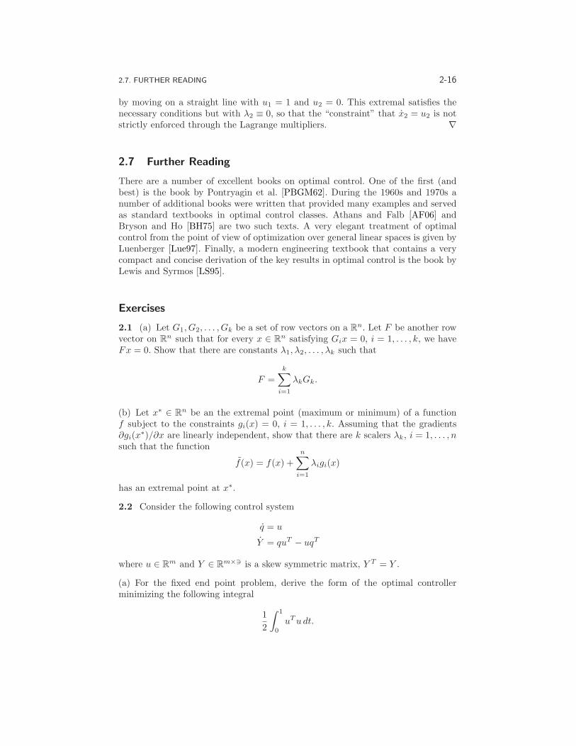
Exercises
2.1 (a) Let G1, G2, . . . , Gk be a set of row vectors on a Rn. Let F be another row
vector on Rn such that for every x ∈ R
n satisfying Gix = 0, i = 1, . . . , k, we haveFx = 0. Show that there are constants λ1, λ2, . . . , λk such that
F =
k∑
i=1
λkGk.
(b) Let x∗ ∈ Rn be an the extremal point (maximum or minimum) of a function
f subject to the constraints gi(x) = 0, i = 1, . . . , k. Assuming that the gradients∂gi(x
∗)/∂x are linearly independent, show that there are k scalers λk, i = 1, . . . , nsuch that the function
f(x) = f(x) +
n∑
i=1
λigi(x)
has an extremal point at x∗.
2.2 Consider the following control system
q = u
Y = quT − uqT
where u ∈ Rm and Y ∈ R
m×∋ is a skew symmetric matrix, Y T = Y .
(a) For the fixed end point problem, derive the form of the optimal controllerminimizing the following integral
1
2
∫ 1
0
uTu dt.

2.7. FURTHER READING 2-17
(b) For the boundary conditions q(0) = q(1) = 0, Y (0) = 0 and
Y (1) =
0 −y3 y2y3 0 −y1−y2 y1 0
for some y ∈ R3, give an explicit formula for the optimal inputs u.
(c) (Optional) Find the input u to steer the system from (0, 0) to (0, Y ) ∈ Rm ×
Rm×m where Y T = −Y .
(Hint: if you get stuck, there is a paper by Brockett on this problem.)
2.3 In this problem, you will use the maximum principle to show that the shortestpath between two points is a straight line. We model the problem by constructinga control system
x = u,
where x ∈ R2 is the position in the plane and u ∈ R
2 is the velocity vector alongthe curve. Suppose we wish to find a curve of minimal length connecting x(0) = x0
and x(1) = xf . To minimize the length, we minimize the integral of the velocityalong the curve,
J =
∫ 1
0
‖x‖ dt =
∫ 1
0
√xT x dt,
subject to to the initial and final state constraints. Use the maximum principle toshow that the minimal length path is indeed a straight line at maximum velocity.(Hint: try minimizing using the integral cost xT x first and then show this alsooptimizes the optimal control problem with integral cost ‖x‖.)
2.4 Consider the optimal control problem for the system
x = −ax+ bu,
where x = R is a scalar state, u ∈ R is the input, the initial state x(t0) is given,and a, b ∈ R are positive constants. (Note that this system is not quite the same asthe one in Example 2.2.) The cost function is given by
J = 12
∫ tf
t0
u2(t) dt+ 12cx
2(tf ),
where the terminal time tf is given and c is a constant.
(a) Solve explicitly for the optimal control u∗(t) and the corresponding state x∗(t)in terms of t0, tf , x(t0) and t and describe what happens to the terminal statex∗(tf ) as c→ ∞.
(b) Show that the system is differentially flat with appropriate choice of output(s)and compute the state and input as a function of the flat output(s).
(c) Using the polynomial basis tk, k = 0, . . . ,M − 1 with an appropriate choiceof M , solve for the (non-optimal) trajectory between x(t0) and x(tf ). Your answershould specify the explicit input ud(t) and state xd(t) in terms of t0, tf , x(t0), x(tf )and t.

2.7. FURTHER READING 2-18
(d) Let a = 1 and c = 1. Use your solution to the optimal control problem andthe flatness-based trajectory generation to find a trajectory between x(0) = 0 andx(1) = 1. Plot the state and input trajectories for each solution and compare thecosts of the two approaches.
(e) (Optional) Suppose that we choose more than the minimal number of basisfunctions for the differentially flat output. Show how to use the additional degreesof freedom to minimize the cost of the flat trajectory and demonstrate that you canobtain a cost that is closer to the optimal.
2.5 Repeat Exercise 2.4 using the system
x = −ax3 + bu.
For part (a) you need only write the conditions for the optimal cost.
2.6 Consider the problem of moving a two-wheeled mobile robot (e.g., a Segway)from one position and orientation to another. The dynamics for the system is givenby the nonlinear differential equation
x = cos θ v, y = sin θ v, θ = ω,
where (x, y) is the position of the rear wheels, θ is the angle of the robot withrespect to the x axis, v is the forward velocity of the robot and ω is spinning rate.We wish to choose an input (v, ω) that minimizes the time that it takes to movebetween two configurations (x0, y0, θ0) and (xf , yf , θf ), subject to input constraints|v| ≤ L and |ω| ≤M .
Use the maximum principle to show that any optimal trajectory consists ofsegments in which the robot is traveling at maximum velocity in either the forwardor reverse direction, and going either straight, hard left (ω = −M) or hard right(ω = +M).
Note: one of the cases is a bit tricky and cannot be completely proven with thetools we have learned so far. However, you should be able to show the other casesand verify that the tricky case is possible.
2.7 Consider a linear system with input u and output y and suppose we wish tominimize the quadratic cost function
J =
∫∞
0
(yT y + ρuTu
)dt.
Show that if the corresponding linear system is observable, then the closed loopsystem obtained by using the optimal feedback u = −Kx is guaranteed to bestable.
2.8 Consider the system transfer function
H(s) =s+ b
s(s+ a), a, b > 0
with state space representation
x =
[0 10 −a
]x+
[01
]u,
y =[b 1
]x

2.7. FURTHER READING 2-19
and performance criterion
V =
∫∞
0
(x21 + u2)dt.
(a) Let
P =
[p11 p12
p21 p22
],
with p12 = p21 and P > 0 (positive definite). Write the steady state Riccati equationas a system of four explicit equations in terms of the elements of P and the constantsa and b.
(b) Find the gains for the optimal controller assuming the full state is available forfeedback.
(c) Find the closed loop natural frequency and damping ratio.
2.9 Consider the optimal control problem for the system
x = ax+ bu J = 12
∫ tf
t0
u2(t) dt+ 12cx
2(tf ),
where x ∈ R is a scalar state, u ∈ R is the input, the initial state x(t0) is given, anda, b ∈ R are positive constants. We take the terminal time tf as given and let c > 0be a constant that balances the final value of the state with the input required toget to that position. The optimal trajectory is derived in Example 2.2.
Now consider the infinite horizon cost
J = 12
∫∞
t0
u2(t) dt
with x(t) at t = ∞ constrained to be zero.
(a) Solve for u∗(t) = −bPx∗(t) where P is the positive solution correspondingto the algebraic Riccati equation. Note that this gives an explicit feedback law(u = −bPx).(b) Plot the state solution of the finite time optimal controller for the followingparameter values
a = 2, b = 0.5, x(t0) = 4,
c = 0.1, 10, tf = 0.5, 1, 10.
(This should give you a total of 6 curves.) Compare these to the infinite time optimalcontrol solution. Which finite time solution is closest to the infinite time solution?Why?
2.10 Consider the lateral control problem for an autonomous ground vehicle fromExample 1.1. We assume that we are given a reference trajectory r = (xd, yd)corresponding to the desired trajectory of the vehicle. For simplicity, we will assumethat we wish to follow a straight line in the x direction at a constant velocity vd > 0and hence we focus on the y and θ dynamics:
y = sin θ vd, θ =1
ltanφ vd.
We let vd = 10 m/s and l = 2 m.

2.7. FURTHER READING B-1
(a) Design an LQR controller that stabilizes the position y to yd = 0. Plot thestep and frequency response for your controller and determine the overshoot, risetime, bandwidth and phase margin for your design. (Hint: for the frequency domainspecifications, break the loop just before the process dynamics and use the resultingSISO loop transfer function.)
(b) Suppose now that yd(t) is not identically zero, but is instead given by yd(t) =r(t). Modify your control law so that you track r(t) and demonstrate the perfor-mance of your controller on a “slalom course” given by a sinusoidal trajectory withmagnitude 1 meter and frequency 1 Hz.