OPTIMIZATION APPROACH AND SOME RESULTS FOR 2D

COMPRESSOR AIRFOIL

Oleg V. Komarov1, Viacheslav A. Sedunin1, Vitaly L. Blinov1, Sergey A. Serkov1 1 The Ural Federal University, Turbines and Engines Department

Yekaterinburg 620000, Russia

v.a.sedunin@gmail.com

ABSTRACT

Several optimization approaches are presented in the paper, and

the results of each task depending on the optimization setup are

compared and discussed in terms of physical behavior and

convergence. The optimization problem is set up and solved for

several 2D compressor airfoils with different inlet parameters. The

airfoils were generated and their characteristics were built for

optimized solutions from different optimization approaches. The

novel topology for 2D compressor airfoil is proposed and

successfully utilized. The approach was tested for particular cases

and showed a gain in efficiency and flow turning up to 15%

(relative) compared with NACA-65 airfoils taken as the initial

design.

INTRODUCTION

Modern axial compressors for Gas Turbine engines are

designed to increase pressure ratios in order to achieve higher

engine efficiencies. Therefore, the loading of the compressor stage

is getting higher to keep the number of stages at a minimum level.

This makes the weight of the aero engines and the footprint for

ground-based GTU as low as possible.

Nowadays optimization techniques play a key role in the design

process of any part of turbomachinery. With the computational

resources becoming more available, the scale of the optimization

problems is also increasing, so the rational approach to

optimization procedure is still of significant interest. In the last

decades inverse design methods [2,3,17] and CFD-based shape

optimization procedures were specifically developed for

turbomachinery applications [6]. The novel optimization concept

followed in the presented research is universal, so it can be applied

to a variety of problems. It can be described as:

1. to structure the model on a physically based way;

2. to solve a series of optimization tasks in a wide range of

working conditions;

3. to systematize the behavior of key design parameters and

define the correlations in the whole design space;

4. to define the series of optimized solutions with the possibility

of further extrapolation;

One should consider the possible problems of this approach,

such as:

1. CFD codes depend on the mesh quality, turbulence modeling

etc. So the model should be properly verified and the working

range should also be defined in reliable way;

2. Extrapolation of the model might need more physical effects

to be considered, also the continuity of design space itself should

be controlled.

With respect to these statements the present work is addressed

to the validation of different optimization approaches. The terms

considered below are parameters that could be included in

objective function, the extent of each parameter range, time of

convergence for optimization task and finally how soon the best

solution is reached.

NOMENCLATURE

b chord length

B control point

C blade thickness

D diameter

G mass flow

M Mach number

F objective function

β angle

ζ pressure losses

γ pressure loss coefficient

i incidence angle

Jn Bezier basis

t coordinate parameter of points on the airfoil

P pressure

w axial velocity

u circumferential velocity

Subscripts

0 initial value

0,1,2,3,4 indexes of control points

i index of the control point; iteration number

in inflow parameters

out outflow parameters

n order of Bezier curve

tot total parameter

Abbreviations

AVDR axial velocity density ratio

OGV outlet guide vane

LE leading edge

PS pressure side

SS suction side

TE trailing edge

GTU Gas Turbine Unit

CDA Controlled Diffusion Airfoil

MCA Multiple Circular Arc

CFD Computation fluid dynamics

PROFILING

In the early 80's the prescribed parameters distribution concept

was implemented in several designs. Hobbs and Weingold [4]

successfully developed a series of CDA’s [Controlled Diffusion

Airfoils] for multistage compressor application. The cascades were

International Journal of Gas Turbine, Propulsion and Power Systems December 2016, Volume 8, Number 3

Manuscript Received on March 2, 2016 Review Completed on November 15, 2016

Copyright © 2016 Gas Turbine Society of Japan

39

designed with an inlet Mach number of 0.7, inlet flow angle of 30°,

flow turning 13.6°, AVDR [define AVDR] 1.07, and solidity of

0.933. Cascade test results demonstrated the lower losses and wider

low-loss incidence range of the CDA’s than conventional

NACA-series airfoils and Multiple Circular Arc (MCA) airfoils. In

addition, single and multistage rig tests showed high efficiency,

high loading capability, and ease of stage matching. The shock-free

and separation-free design concept for CDA’s had been proved.

Behlke [5] extended the basic CDA philosophy to the end wall flow

region and developed new CDA’s for multistage compressors. The

results showed a 1.5% increase in efficiency and 30% increase in

surge-free operation compared to original CDAs’ designed by

Hobbs and Weingold.

Due to the superior aerodynamic performance, CDA aroused

considerable research interest around the world [7] and became a

part of design process in leading companies [8]. The main

challenge in this approach is that every single CDA airfoil working

with different flow condition is a particular case solved and

optimized for exact requirements. So it takes significant effort to

unify and compile the result with traditional techniques and

programs for multistage compressor design using common fast and

rapid 1D and 2D algorithms based on traditional airfoils. Though,

standardized topology for controlled diffusion airfoils with proper

loss characteristics is needed. Also an interesting approach for the

profiling is shown in [14].

The 2D mid-span airfoil of the compressor cascade is presented

in Figure 1 in dots. Detailed physical explanation and advantages

are discussed in details in [9].

Two Bezier curves form pressure and suction side and two arcs

represent leading and trailing edges. All curves are tangential to its

neighbors in point of contact. The suction side curve is formed by

3rd order Bezier curve, whereas pressure side is 4th order. The

schematic view of the 2D section is presented in Figure 1.

There are three types of geometry parameters, defined in the

project:

1. Design constraints that are similar in all airfoils, considered

during optimization process. These are: fixed reference point at

LE (point B3ss) and fixed axial length of the profile.

2. Controlled parameters (varied with the optimization code

during the process). From geometrical point of view these

parameters are used in airfoil profiling algorithm to build a

unique determined shape. These parameters are: axial position

of points B1ss, B2ss, B1ps, B3ps circumferential position of B0ss,

angles of lines between control points: B3ss - B2ss, B0ps- B1ps etc

(this lines are tangent to LE or TE and therefore represents

blade angle β1 and β2 on suction and pressure sides); also point

B2ps can be varied both in axial and circumferential directions.

As a result 11 parameters are controlled by optimization

algorithm.

3. Calculated parameters (computed within the codes) are also

very important during the overall process. Such as: maximum

and minimum thickness of the blade, position of max thickness,

stagger angle, moment of inertia etc.

The profile shape itself is described by two arcs (LE and TE) and

two Bezier curves that can be mathematically presented according

to [10]:

(1)

Where Bi – is i-vertex of Bezier polygon, Jn - Bezier basis

(Bernstein basis or approximation function), which can be

computed with:

(2)

- is i-function of Bernstein basis with order n. Here 'n' –

order of definition function of Bernstein basis and therefore of

segment of the polynomial curve. 'n' is one less than number of

vertexes in defining polygon. Bezier polygon is numbered from 0 to

n1.

The suction side is formed by 3rd order Bezier curve (n=3), the

pressure side - 4th order (Figure1).

Coefficient for 3rd order Bezier curve can be described as follows:

(3)

Fig. 1. Airfoil topology using Bezier curves

JGPP Vol.8, No. 3

40

Parametrical equation for 3rd order Bezier curve is as follows:

4th order Bezier curve has similar topology according to [10].

So by controlling of parameter 't' one can obtain coordinates of

all points on the SS and PS curves.

This basic representation is mostly traditional but has some

physical background, which helps to arrange the optimization

procedure in more effective way. So not just a blind generic

algorithm is used, but physically explained parameters are

implemented and therefore some logical expectations might be

assumed.

The physical interpretation is the following: Blade can be

conceptually splitted in three sections (Figure 1). Suction side:

section I on SS: in point B2ss the angle between line B2ss and frontal

surface represent the inlet angle of the blade from suction side

βin(ss). This parameter can be used for control and adaptation of the

profile for positive incidence angle (βinflow < βin(nominal)). Axial

position of B2ss controls the length and curvature of a smooth

transition region at SS after leading edge, because this part is

known to affect the boundary layer behavior (eg. laminar -

turbulent boundary layer transition). It is expected that B2ss will be

defined mostly by Reynolds and Mach number.

Section II+III on SS: Angle between line B1ss - B0ss and front

surface is Betta 2 from suction side (β2ss) and axial position of B1ss

defines rear load on the profile outflow region at SS by changing

the curvature of this part.

Section I PS: As for point 1ss tangential condition with leading

edge is applied and therefore line B0ps- B1ps has an angle to the front

surface equals to β1ps. The length of this segment is controlled by

the axial position of control point B1ps. These two parameters affect

the characteristics of the profile at high mass flow modes (far right

side of the compressor speed line). Also this part can affect the

throat of the channel.

Table 1. Parameters for airfoils similar to NACA-65 series.

Variable Coordinates

of control points in

mm or degrees0

Initial value

1 2 3

X B1ps

17.73 20.56 21.48

X B2ps

30.09 32.91 33.82

Y B2ps

7.07 7.53 7.13

X B3ps

42.44 45.25 46.16

Y B0ss

26.12 16.40 12.10

X B1ss

37.67 40.70 41.64

X B2ss

21.23 24.03 25.07

in(ps) 37.28 37.42 37.48

in(ss) 57.77 56.13 55.19

out(ps) 34.93 15.71 5.94

out(ss) 29.99 12.06 2.71

Section II PS: this is needed only for geometrical matching of

pressure and suction sides with minimal trailing edge thickness. It

can be explained by the fact that average surface angle (medium

between βin(ss) and βout(ss)) at SS is lower than this can be achieved

for PS and is limited by flow separation conditions, whereas at PS

there are not so many reasons to decrease this parameter. Therefore

these two lines (PS and SS) go in opposite directions and will never

meet each other if no geometrical constraints would be

implemented.

Section III PS: Outlet region of the blade. It is known that

outflow angle β2 cannot exceed β2ps. Therefore maximum stagger

angle for this curve is desired, but again geometry constraints

should be considered. In [5] it is shown that outlet region also can

be used for artificial increasing of βout(ss) by implementation of

"bulb-shape" at profile exit. To let the optimization algorithm test

this feature in wide range of inflow parameters, 3 control points

were used to describe the pressure side curve.

As initial for every optimization process the NACA-65 airfoil

series were used with circular camber line and equal thickness.

Dedicated algorithm was used to describe these NACA airfoils with

the presented topology. In Table 1 parameters for the initial airfoil

design are presented.

VERIFICATION

Mesh parameters (Figure 2), boundary conditions and

turbulence model were previously tested on compressor airfoil

10A40/15П45 which was widely tested by Bunimovich [11]. Inlet

Mach number range is from 0.4 to 0.75, incidence angle -7.5 to 12

degrees. Also for low Mach number data from [12] was used which

is devoted to NACA series airfoils.

CFD computations and post-processing was performed in

ANSYS CFX, turbulence model k-epsilon standard. y+ 20, wall

function - scalable. Boundary conditions: hub and shroud are

considered as free slip walls; blade surface - no slip wall with 3 μm

roughness. Mesh Topology - ATM Optimized. Total mesh size of

the domain - 250 000 cells. Total pressure and temperature at inlet

together with inlet velocity vector components; Static pressure at

outlet. The pressure drop was chosen to achieve necessary Mach

number at the current operating point. The domain has extension of

20% of blade chord at inlet and 100% of chord after the blade.

The parameters are computed using mass flow averaged

parameters at inlet and outlet sections of the computational domain.

As a result flow turning angle and pressure losses over the

whole range were evaluated and compared with experimental data

(Figure 3). As a result one can see that at nominal mode the

computation results lay higher than experimental ones. but at the

high incidence angle the model behavior is more optimistic than

experiment. In general these results and deviations are comparable

with ones with [13]. In this reference the pressure loss coefficient

was computed as: tot tot

in out

tot

in

P P

P

(4)

where Pintot and Pout

tot – are mass flow averaged total pressures at

the computational domain inlet and outlet respectively.

Since the optimization procedure itself taking and processing

initial design with the same CFD parameters and further

improvement is related to initial state the verification results are

considered as acceptable for further research keeping in mind the

necessity for improvement.

Fig.2 Fragment of the structured mesh at the leading and

trailing edges of the profile

JGPP Vol.8, No. 3

41

Fig. 3 Verification of CFD model

OPTIMIZATION PROCEDURE

The optimization process is presented on Figure 4 and is

realized in the IOSO software [15,16] in connection with the

relevant ANSYS modules and in-house profiling code.

By using the topology described above the profile was

generated, checked for geometry and structural constraints and

exported to ANSYS. Then the computation was performed at two

modes: +3 and -3 degrees incidence from the blade inlet angle.

In this way it is possible to control the improvement of an

airfoil together with maintaining the necessary working range. The

range itself corresponds to stable working parameters, where the

model shows good correlation with experiment.

Here the +3 degrees mean the incidence from pressure side and

degrees are measured from frontal surface. So for example, if the

blade inlet angle for initial NACA design is 45 degrees, the inflow

angles during optimization will be 48 and 42 degrees. The range of

6 degrees is considered acceptable and achievable for inlet Mach

number 0.6. Boundary details were done as it is in the verified

model.

Then the computation results were transferred to IOSO

software to be processed and analyzed in order to generate new set

of geometry parameters for the next iteration.

The IOSO method is a constrained optimization algorithm

based on response surface methods and evolutionary computation

principles. Each iteration of IOSO consist of two steps. The first

step is creation of an approximation of the objective function(s).

Each iteration in this step represents a decomposition of an initial

approximation function into a set of simple approximation

Fig. 4 Schematic representation of iterative optimization process

functions. The final response function is a multilevel graph. The

second step is the optimization of this approximation function. This

approach allows for self-corrections of the structure and the

parameters of the response surface approximation. The distinctive

feature of this approach is an extremely low number of trial points

to initialize the algorithm [15].

OBJECTIVE AND CONSTRAINTS

In this section the design objective and constraint functions are

detailed. The objective of the design optimization is to maximize

the flow turning angle in the cascade together with minimum

pressure losses. Since the two modes optimization takes place the

key question is how to estimate the importance of each parameter to

the final result. This question opens up a large space for

investigation and there were three possible approaches converted to

three types of tasks. and therefore objective functions:

1. Minimum losses at both modes and maximum flow turning

angle at +3 incidence;

2. Minimum losses at both modes and maximum flow turning

angle at both modes (the function itself presented at eq.6);

3. Minimum losses at both modes and fixed flow turning angle.

This task was launched for three different blade camber line turning

angles: 15, 33 and 42 degrees. The range of optimization

parameters is presented in Table 2.

For first and second tasks the initial design is presented in table

1, airfoil №1. For the 3rd task every sub-task had its own initial

geometry built from NACA-65 series depending on the expected

turning angle.

JGPP Vol.8, No. 3

42

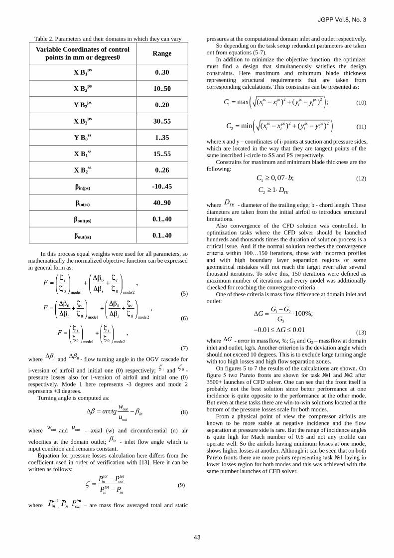
Table 2. Parameters and their domains in which they can vary

Variable Coordinates of control

points in mm or degrees0 Range

X B1ps

0..30

X B2ps

10..50

Y B2ps

0..20

X B3ps

30..55

Y B0ss

1..35

X B1ss

15..55

X B2ss

0..26

βin(ps) -10..45

βin(ss) 40..90

βout(ps) 0.1..40

βout(ss) 0.1..40

In this process equal weights were used for all parameters, so

mathematically the normalized objective function can be expressed

in general form as:

(5)

(6)

(7)

where i and 0 - flow turning angle in the OGV cascade for

i-version of airfoil and initial one (0) respectively; i and 0 -

pressure losses also for i-version of airfoil and initial one (0)

respectively. Mode 1 here represents -3 degrees and mode 2

represents +3 degrees.

Turning angle is computed as:

out

in

out

warctg

u (8)

where outwand outu

- axial (w) and circumferential (u) air

velocities at the domain outlet; in - inlet flow angle which is

input condition and remains constant.

Equation for pressure losses calculation here differs from the

coefficient used in order of verification with [13]. Here it can be

written as follows:

tot tot

in out

tot

in in

P P

P P

(9)

where . . – are mass flow averaged total and static

pressures at the computational domain inlet and outlet respectively.

So depending on the task setup redundant parameters are taken

out from equations (5-7).

In addition to minimize the objective function, the optimizer

must find a design that simultaneously satisfies the design

constraints. Here maximum and minimum blade thickness

representing structural requirements that are taken from

corresponding calculations. This constrains can be presented as:

2 2

1 max ( ) ( ) ;ss ps ss ps

i i i iC x x y y (10)

2 2

2 min ( ) ( )ss ps ss ps

i i i iC x x y y (11)

where x and y – coordinates of i-points at suction and pressure sides,

which are located in the way that they are tangent points of the

same inscribed i-circle to SS and PS respectively.

Constrains for maximum and minimum blade thickness are the

following:

1 0,07 ;C b (12)

2 1 TEC D

where - diameter of the trailing edge; b - chord length. These

diameters are taken from the initial airfoil to introduce structural

limitations.

Also convergence of the CFD solution was controlled. In

optimization tasks where the CFD solver should be launched

hundreds and thousands times the duration of solution process is a

critical issue. And if the normal solution reaches the convergence

criteria within 100…150 iterations, those with incorrect profiles

and with high boundary layer separation regions or some

geometrical mistakes will not reach the target even after several

thousand iterations. To solve this, 150 iterations were defined as

maximum number of iterations and every model was additionally

checked for reaching the convergence criteria.

One of these criteria is mass flow difference at domain inlet and

outlet:

1 2

2

100%;

0.01 0.01

G GG

G

G

(13)

where - error in massflow, %; G1 and G2 – massflow at domain

inlet and outlet, kg/s. Another criterion is the deviation angle which

should not exceed 10 degrees. This is to exclude large turning angle

with too high losses and high flow separation zones.

On figures 5 to 7 the results of the calculations are shown. On

figure 5 two Pareto fronts are shown for task №1 and №2 after

3500+ launches of CFD solver. One can see that the front itself is

probably not the best solution since better performance at one

incidence is quite opposite to the performance at the other mode.

But even at these tasks there are win-to-win solutions located at the

bottom of the pressure losses scale for both modes.

From a physical point of view the compressor airfoils are

known to be more stable at negative incidence and the flow

separation at pressure side is rare. But the range of incidence angles

is quite high for Mach number of 0.6 and not any profile can

operate well. So the airfoils having minimum losses at one mode,

shows higher losses at another. Although it can be seen that on both

Pareto fronts there are more points representing task №1 laying in

lower losses region for both modes and this was achieved with the

same number launches of CFD solver.

JGPP Vol.8, No. 3

43

a.

b.

Fig. 5 Series of optimized solutions (a) incidence (-3) degrees. (b)

incidence (+3) degrees.

For both modes best results turning angle exceed 30 degrees

and these results are by 2-3 degrees higher for Task-1 than ones for

Task-2.

In the red dot the initial design is shown. Here it is just a

reference point whereas in figure 6 the improvement shows lower

losses with the turning angle remaining at the same level. So the

improvement is more specific and the Pareto front is more likely to

converge. Each sub-task takes over 1500 iterations.

Also at figure 6 several points are taken from task 1 and 2 for

more detailed comparison and understanding of the speed of

convergence for different tasks. In the sub-task 3-1 the

improvement in losses is 0.5% absolute for one mode and 0.2% for

another comparing to initial NACA airfoil. For sub-tasks 3-2 and

3-3 the improvements are 0.6% and 0.8% at one mode and 3.5%

and 5.6% at another mode respectively.

To compare the results from task 1, 2 and 3 on figure 6 there are

several points from task 1 and 2 chosen from overall Pareto fronts

with the same (approximately) turning angles. It can be seen, that

these points are lying in the general Pareto from task 3. Taking into

account the computation time and the width of optimized solutions

the most preferable task setup seems to be task №1.

One of the most important questions is when the task can be

considered as converged. On figure 7 the convergence of

optimization task 3-1 is shown. The vertical part of Pareto front is

coming to its near-best state within the first 300 iterations whereas

the middle and horizontal parts continue improvement even after

1500+ iterations (launches of CFD solver).

Figure 6. Pareto front for task 3 (3-1 is for 15 degrees initial

camber turning angle. 3-2 - 33deg. 3-3 - 42 deg).

OPTIMIZATION RESULTS

On figure 8 the comparisons of initial and optimized

geometries for different tasks are given. On figure 9 one can see the

characteristics of the airfoils.

On figures 9 and 10 the following numbering is used: Task-1-1

means that from Pareto Front of Task 1 the point was chosen with

the turning angle close to 15 degrees which is similar to Task-3-1.

Remember that Task-3 means losses minimization for specific flow

turn and it is important to compare airfoils with equal flow turn.

The same principle for Task-1-2 – it is stated for turning angle

around 15 degrees but is taken from Pareto front 2.

On Figure 9 one can see that pressure losses in optimized

profiles are lower than in initial together with equal or higher

turning angle. The best gain can be seen in Figure 9a. Also the

working range becomes wider up to 30% (by the working range it is

assumed the space where the pressure loss is not exceeding double

of minimum loss).

On Figure 10 local Mach number distributions along the airfoil

are presented for the following airfoils: NACA-1 (which is

NACA-65 series for 15 deg. turning), Task-1-1, the point taken

from Pareto front of the task 1, similar to NACA-1 turning;

Task-1-2 and Task-1-3 respectively. These airfoils are shown at

Figure 8a and its characteristics are at Figure 9a. Inlet Mach

number is equal for all cases here.

Here one should notice, that two modes that were considered as

+3 and -3 incidence angle are not necessary the same for every

profile presented on the Pareto front. The resulting airfoil can be

oriented as +2/-4 or +6/0 for these two modes. And therefore losses

and turning angle to be compared in the whole range. For example,

stagger angle for profile 1-1 (Fig.8a) is higher than three others on

the same graph. This gives the velocity distribution shown at figure

10b.

Fig.7 Convergence of optimization task 3-1.

JGPP Vol.8, No. 3

44

a.

b.

c.

Fig. 8 Comparison of optimized airfoils with NACA-1 (a).

NACA-2 (b) and NACA-3 (c).

CONCLUSIONS

The topology of CDA compressor airfoils is presented and their

parameters are explained from both geometrical and fluid dynamics

aspects. It is very important that. while optimization procedure

itself provides win-to-win solution for only one exact blade profile.

the structured topology of the airfoil together with modern CFD

and optimization algorithms can be used to elaborate a family of

best profiles covering a whole range of compressor flow

parameters.

The in-house code allows controlling critical geometry

parameters such as thickness, LE and TE radius, moment of inertia

and others, so this approach is very convenient for application in

complex design systems.

During the optimization process the operating range of an

airfoil is one of the hardest criteria to maintain and it should be

considered according to the overall compressor requirements.

In the current research the range of 6 degrees was kept for inlet

Mach number of 0.6. The most suitable problem statement for

multimodal optimization of 2D compressor airfoil is maximum

turning angle at incidence from pressure side and minimum losses

at all modes.

a.

b.

c.

Fig. 9 Airfoil characteristic for different flow turning: NACA-1

(a). NACA-2 (b) and NACA-3 (c).

In spite of the fact that most of the world modern compressors

contain supersonic and transonic stages at the inlet, the middle and

rear stages remain subsonic. So, increased loading together with

predictable performance over the whole load range remains very

important.

When a double mode optimization task is set up, a wide range

of flow parameters should be studied for the same

problem-definition in order to discover logical correlation between

flow and blade parameters.

The most suitable problem definition includes three

optimization criteria: minimum losses at both modes and maximum

turning angle at maximum load (minimum flow coefficient). This

approach gives relatively high speed together with guaranteed

working range of an airfoil.

Also, the computational model parameters, such as CFD solver

details (turbulence models. mesh parameters etc.) and optimization

approaches are always subject for discussion. therefore a

significant effort needs to be made in future to verify this topology

based approach with different solvers and optimization techniques.

JGPP Vol.8, No. 3

45

a.

b.

c.

d.

Fig. 10 Local Mach number distributions for airfoils: NACA-1 (a).

Task-1-1 (b). Task-1-2 (c) and Task-1-3 (d).

ACKNOWLEDGMENTS

This work is carried out with support of The Ural Federal

University foundation within the Program of Development.

References

[1] Cumpsty N.A.. 2004. Compressor Aerodynamics. Krieger

Publishing Company. 2004

[2] Leonard. O.. and Van Den Braembussche. R.. 1992. “Design

Method for Subsonic and Transonic Cascade With Prescribed

Mach Number Distribution”. Journal of Turbomachinery.

114(3). p. 553.

[3] Shahpar. S.. and Lapworth. L.. 2003. Padram: Parametric

design and rapid meshing system for turbomachinery

optimisation. ASME Turbo Expo GT2003-38698. Atlanta.

Georgia. USA.

[4] Hobbs. D. E.. and Weingold. H. D.. “Development of

Controlled Diffusion Airfoils for Multistage Compressor

Application.” Journal of Engineering for Gas Turbines and

Power. Vol. 106. pp. 271-278. 1984.

[5] Behlke. R.F.. “The development of a Second Generation of

Controlled Diffusion Airfoils for Multistage Compressors.”

Journal of Turbomachinery. Vol. 108. pp. 32-41. 1986.

[6] Pini M.. Persico G.. Dossena V. 2014 "Robust adjointbased

shape optimization of supersonic turbomachinery cascades".

GT2014-27064. Proceedings of ASME Turbo Expo. June

16-20. 2014. Dusseldorf. Germany.

[7] Song B.. 2003. "Experimental and Numerical Investigations

of Optimized High-Turning Supercritical Compressor

Blades." Doctoral thesis. Virginia Polytechnic Institute an

State University. pp.155.

[8 Smith L.H.. 2002. "Axial compressor aerodesign evolution at

General Electric" ASME Journal of Turbomachinery. vol.

124.

[9] Sedunin V.A.. Blinov V.L.. Komarov O.V. 2014 "Application

of optimisation techniques for new high-turning axial

compressor profile topology design". GT2014-25379.

Proceedings of ASME Turbo Expo. June 16-20. 2014.

Dusseldorf. Germany.

[10] Rogers. David F. and J. Alan Adams. 1990. "Mathematical

Elements for Computer Graphics." second edition. McGraw

Hill. New York. NY. pp. 611.

[11] Bunimovich A.I.. Svyatogorov A.A. 1967

"Aerodinamicheskie charakteristiki ploskyh kompressornyh

reshotok pri bolshoi dozvukovoi skorosti". M.

[12] Emery J.C.. Herrig L.J.. Erwin J.R.. Felix A.R. Systematic

two-dimensional cascade test of NACA 65-series compressor

blades at low speeds. NACA Report 1368. 1958.

Mashinostroyenie. Lopatochnye mashiny i struinye apparaty.

pp.5-36.

[13] Fischer. S.. Müller. L.. Saathoff. H.. Kožulovic. D.. 2012.

"Three-dimensional flow through a compressor cascade with

circulation control". GT2012-68593. Proceedings of ASME

Turbo Expo. June 11-15. 2012. Copenhagen. Denmark.

[14] Bode. С.. Kozulovic. D.. Stark. U.. Hoheisel. H.. 2012.

"Performance and boundary layer development of a high

turning compressor cascade at sub- and supercritical flow

conditions". GT2012-68382. Proceedings of ASME Turbo

Expo. June 11-15. 2012. Copenhagen. Denmark.

[15] Egorov. I.N.. Kretinin. G.V.. Leshchenko. I.A. and

Kuptzov.S.V.. 2002. "IOSO Optimization Toolkit - Novel

Software to Create Better Design." 9th AIAA/ISSMO

Symposium on Multidisciplinary Analysis and Optimization.

04 - 06 Sep. 2002. Atlanta. Georgia.

[16] Egorov I.N.. Kretinin G.V.. Leshchenko I.A.. 1997. “Optimal

Designing and Control of Gas-Turbine Engine Components.

Multicriteria Approach". MCB University Press. Aircraft

Engineering and Aerospace Technology. ISSN 0002-2667.

Vol.69. N 6. pp.518-526.

[17] Boiko A.V.. Govorushenko U.N.. Erchov S.V.. Rusanov A.V..

Severin S.D.. 2002. “Aerodinamicheskiy raschet I

optimalnoe proectirovanie protochnoy chasty turbomachin.”

Charkiv: NTU “ChPI”. pp. 356.

JGPP Vol.8, No. 3

46