OPTIMIZATION AND CONTROL

Richard Weber

Contents

DYNAMIC PROGRAMMING 1

1 Dynamic Programming: The Optimality Equation 11.1 Control as optimization over time . . . . . . . . . . . . . . . . . . . . . . 11.2 The principle of optimality . . . . . . . . . . . . . . . . . . . . . . . . . 11.3 Example: the shortest path problem . . . . . . . . . . . . . . . . . . . . 11.4 The optimality equation . . . . . . . . . . . . . . . . . . . . . . . . . . . 21.5 Markov decision processes . . . . . . . . . . . . . . . . . . . . . . . . . . 4

2 Some Examples of Dynamic Programming 52.1 Example: managing spending and savings . . . . . . . . . . . . . . . . . 52.2 Example: exercising a stock option . . . . . . . . . . . . . . . . . . . . . 62.3 Example: accepting the best offer . . . . . . . . . . . . . . . . . . . . . . 7

3 Dynamic Programming over the Infinite Horizon 93.1 Discounted costs . . . . . . . . . . . . . . . . . . . . . . . . . . . . . . . 93.2 Example: job scheduling . . . . . . . . . . . . . . . . . . . . . . . . . . . 93.3 The infinite-horizon case . . . . . . . . . . . . . . . . . . . . . . . . . . . 103.4 The optimality equation in the infinite-horizon case . . . . . . . . . . . . 113.5 Example: selling an asset . . . . . . . . . . . . . . . . . . . . . . . . . . 12

4 Positive Programming 134.1 Example: possible lack of an optimal policy. . . . . . . . . . . . . . . . . 134.2 Characterization of the optimal policy . . . . . . . . . . . . . . . . . . . 134.3 Example: optimal gambling . . . . . . . . . . . . . . . . . . . . . . . . . 144.4 Value iteration . . . . . . . . . . . . . . . . . . . . . . . . . . . . . . . . 144.5 Example: pharmaceutical trials . . . . . . . . . . . . . . . . . . . . . . . 15

5 Negative Programming 175.1 Stationary policies . . . . . . . . . . . . . . . . . . . . . . . . . . . . . . 175.2 Characterization of the optimal policy . . . . . . . . . . . . . . . . . . . 175.3 Optimal stopping over a finite horizon . . . . . . . . . . . . . . . . . . . 185.4 Example: optimal parking . . . . . . . . . . . . . . . . . . . . . . . . . . 18

i

5.5 Optimal stopping over the infinite horizon . . . . . . . . . . . . . . . . . 19

6 Average-cost Programming 216.1 Average-cost optimization . . . . . . . . . . . . . . . . . . . . . . . . . . 216.2 Example: admission control at a queue . . . . . . . . . . . . . . . . . . . 226.3 Value iteration bounds . . . . . . . . . . . . . . . . . . . . . . . . . . . . 236.4 Policy improvement . . . . . . . . . . . . . . . . . . . . . . . . . . . . . 23

LQG SYSTEMS 25

7 LQ Models 257.1 The LQ regulation model . . . . . . . . . . . . . . . . . . . . . . . . . . 257.2 The Riccati recursion . . . . . . . . . . . . . . . . . . . . . . . . . . . . . 277.3 White noise disturbances . . . . . . . . . . . . . . . . . . . . . . . . . . 277.4 LQ regulation in continuous-time . . . . . . . . . . . . . . . . . . . . . . 28

8 Controllability 298.1 Controllability . . . . . . . . . . . . . . . . . . . . . . . . . . . . . . . . 298.2 Controllability in continuous-time . . . . . . . . . . . . . . . . . . . . . . 318.3 Example: broom balancing . . . . . . . . . . . . . . . . . . . . . . . . . 318.4 Example: satellite in a plane orbit . . . . . . . . . . . . . . . . . . . . . 32

9 Infinite Horizon Limits 339.1 Linearization of nonlinear models . . . . . . . . . . . . . . . . . . . . . . 339.2 Stabilizability . . . . . . . . . . . . . . . . . . . . . . . . . . . . . . . . . 339.3 Example: pendulum . . . . . . . . . . . . . . . . . . . . . . . . . . . . . 349.4 Infinite-horizon LQ regulation . . . . . . . . . . . . . . . . . . . . . . . . 349.5 The [A, B, C] system . . . . . . . . . . . . . . . . . . . . . . . . . . . . . 36

10 Observability 3710.1 Observability . . . . . . . . . . . . . . . . . . . . . . . . . . . . . . . . . 3710.2 Observability in continuous-time . . . . . . . . . . . . . . . . . . . . . . 3810.3 Examples . . . . . . . . . . . . . . . . . . . . . . . . . . . . . . . . . . . 3910.4 Imperfect state observation with noise . . . . . . . . . . . . . . . . . . . 40

11 Kalman Filtering and Certainty Equivalence 4111.1 Preliminaries . . . . . . . . . . . . . . . . . . . . . . . . . . . . . . . . . 4111.2 The Kalman filter . . . . . . . . . . . . . . . . . . . . . . . . . . . . . . 4111.3 Certainty equivalence . . . . . . . . . . . . . . . . . . . . . . . . . . . . . 4211.4 Example: inertialess rocket with noisy position sensing . . . . . . . . . . 43

CONTINUOUS-TIME MODELS 45

ii

12 Dynamic Programming in Continuous Time 4512.1 The optimality equation . . . . . . . . . . . . . . . . . . . . . . . . . . . 4512.2 Example: LQ regulation . . . . . . . . . . . . . . . . . . . . . . . . . . . 4612.3 Example: estate planning . . . . . . . . . . . . . . . . . . . . . . . . . . 4612.4 Example: harvesting . . . . . . . . . . . . . . . . . . . . . . . . . . . . . 47

13 Pontryagin’s Maximum Principle 4913.1 Heuristic derivation . . . . . . . . . . . . . . . . . . . . . . . . . . . . . . 4913.2 Example: bringing a particle to rest in minimal time . . . . . . . . . . . 5013.3 Connection with Lagrangian multipliers . . . . . . . . . . . . . . . . . . 5113.4 Example: use of the transversality conditions . . . . . . . . . . . . . . . 52

14 Applications of the Maximum Principle 5314.1 Problems with terminal conditions . . . . . . . . . . . . . . . . . . . . . 5314.2 Example: monopolist . . . . . . . . . . . . . . . . . . . . . . . . . . . . . 5414.3 Example: insects as optimizers . . . . . . . . . . . . . . . . . . . . . . . 5414.4 Example: rocket thrust optimization . . . . . . . . . . . . . . . . . . . . 55

15 Controlled Markov Jump Processes 5715.1 The dynamic programming equation . . . . . . . . . . . . . . . . . . . . 5715.2 The case of a discrete state space . . . . . . . . . . . . . . . . . . . . . . 5715.3 Uniformization in the infinite horizon case . . . . . . . . . . . . . . . . . 5815.4 Example: admission control at a queue . . . . . . . . . . . . . . . . . . . 59

16 Controlled Diffusion Processes 6116.1 Diffusion processes and controlled diffusion processes . . . . . . . . . . . 6116.2 Example: noisy LQ regulation in continuous time . . . . . . . . . . . . . 6216.3 Example: a noisy second order system . . . . . . . . . . . . . . . . . . . 6216.4 Example: passage to a stopping set . . . . . . . . . . . . . . . . . . . . . 63

Index 65

Schedules

The first 6 lectures are devoted to dynamic programming in discrete-time andcover both finite and infinite-horizon problems; discounted-cost, positive, negative andaverage-cost programming; the time-homogeneous Markov case; stopping problems;value iteration and policy improvement.

The next 5 lectures are devoted to the LQG model (linear systems, quadratic costs)and cover the important ideas of controllability and observability; the Ricatti equation;imperfect observation, certainly equivalence and the Kalman filter.

The final 5 lectures are devoted to continuous-time models and include treatmentof Pontryagin’s maximum principle and the Hamiltonian; Markov decision processes ona countable state space and controlled diffusion processes.

iii

Each of the 16 lectures is designed to be a somewhat self-contained unit, e.g., therewill be one lecture on ‘Negative Programming’, one on ‘Controllability’, etc. Examplesand applications are important in this course, so there are one or more worked examplesin each lecture.

Examples sheets

There are three examples sheets, corresponding to the thirds of the course. There aretwo or three questions for each lecture, some theoretical and some of a problem nature.Each question is marked to indicate the lecture with which it is associated.

Lecture Notes and Handouts

There are printed lecture notes for the course and other occasional handouts. Thereare sheets summarising notation and what you are expected to know for the exams.

The notes include a list of keywords and I will be drawing your attention to these aswe go along. If you have a good grasp of the meaning of each of these keywords, thenyou will be well on your way to understanding the important concepts of the course.

WWW pages

Notes for the course, and other information are on the web athttp://www.statslab.cam.ac.uk/~rrw1/oc/index.html.

Books

The following books are recommended.

D. P. Bertsekas, Dynamic Programming, Prentice Hall, 1987.D. P. Bertsekas, Dynamic Programming and Optimal Control,Volumes I and II, Prentice Hall, 1995.L. M. Hocking, Optimal Control: An introduction to the theory and applications, Oxford1991.S. Ross, Introduction to Stochastic Dynamic Programming, Academic Press, 1983.P. Whittle, Optimization Over Time. Volumes I and II, Wiley, 1982-83.

Ross’s book is probably the easiest to read. However, it only covers Part I of thecourse. Whittle’s book is good for Part II and Hocking’s book is good for Part III. Therecent book by Bertsekas is useful for all parts. Many other books address the topics ofthe course and a collection can be found in Sections 3B and 3D of the DPMMS library.Notation differs from book to book. My notation will be closest to that of Whittle’sbooks and consistent throughout. For example, I will always denote a minimal costfunction by F (·) (whereas, in the recommended books you will find F , V , φ, J andmany others symbols used for this quantity.)

iv

1 Dynamic Programming: The Optimality Equation

We introduce the idea of dynamic programming and the principle of optimality. Wegive notation for state-structured models, and introduce ideas of feedback, open-loop,and closed-loop controls, a Markov decision process, and the idea that it can be usefulto model things in terms of time to go.

1.1 Control as optimization over time

Optimization is a key tool in modelling. Sometimes it is important to solve a prob-lem optimally. Other times either a near-optimal solution is good enough, or the realproblem does not have a single criterion by which a solution can be judged. However,even then optimization is useful as a way to test thinking. If the ‘optimal’ solution isridiculous it may suggest ways in which both modelling and thinking can be refined.

Control theory is concerned with dynamic systems and their optimization overtime. It accounts for the fact that a dynamic system may evolve stochastically andthat key variables may be unknown or imperfectly observed (as we see, for instance, inthe UK economy).

This contrasts with optimization models in the IB course (such as those for LP andnetwork flow models); these static and nothing was random or hidden. It is these threenew features: dynamic and stochastic evolution, and imperfect state observation, thatgive rise to new types of optimization problem and which require new ways of thinking.

We could spend an entire lecture discussing the importance of control theory andtracing its development through the windmill, steam governor, and so on. Such ‘classiccontrol theory’ is largely concerned with the question of stability, and there is much ofthis theory which we ignore, e.g., Nyquist criterion and dynamic lags.

1.2 The principle of optimality

A key idea is that optimization over time can often be regarded as ‘optimization instages’. We trade off our desire to obtain the lowest possible cost at the present stageagainst the implication this would have for costs at future stages. The best actionminimizes the sum of the cost incurred at the current stage and the least total cost thatcan be incurred from all subsequent stages, consequent on this decision. This is knownas the Principle of Optimality.

Definition 1.1 (Principle of Optimality) From any point on an optimal trajectory,the remaining trajectory is optimal for the corresponding problem initiated at that point.

1.3 Example: the shortest path problem

Consider the ‘stagecoach problem’ in which a traveler wishes to minimize the lengthof a journey from town A to town J by first traveling to one of B, C or D and thenonwards to one of E, F or G then onwards to one of H or I and the finally to J. Thusthere are 4 ‘stages’. The arcs are marked with distances between towns.

1

A

B

C

D

E

F

G

H

I

J

1

1

2

2

3

3

3

33

3

4

4

4

4

4

4

5

6

6

7

Road system for stagecoach problem

Solution. Let F (X) be the minimal distance required to reach J from X. Then clearly,F (J) = 0, F (H) = 3 and F (I) = 4.

F (F) = min[ 6 + F (H), 3 + F (I) ] = 7 ,

and so on. Recursively, we obtain F (A) = 11 and simultaneously an optimal route, i.e.,A→D→F→I→J (although it is not unique).

The study of dynamic programming dates from Richard Bellman, who wrote thefirst book on the subject (1957) and gave it its name. A very large number of problemscan be treated this way.

1.4 The optimality equation

The optimality equation in the general case. In discrete-time t takes integervalues, say t = 0, 1, . . . . Suppose ut is a control variable whose value is to be chosen attime t. Let Ut−1 = (u0, . . . , ut−1) denote the partial sequence of controls (or decisions)taken over the first t stages. Suppose the cost up to the time horizon h is given by

C = G(Uh−1) = G(u0, u1, . . . , uh−1) .

Then the principle of optimality is expressed in the following theorem.

Theorem 1.2 (The principle of optimality) Define the functions

G(Ut−1, t) = infut,ut+1,...,uh−1

G(Uh−1) .

Then these obey the recursion

G(Ut−1, t) = infut

G(Ut, t + 1) t < h ,

with terminal evaluation G(Uh−1, h) = G(Uh−1).

The proof is immediate from the definition of G(Ut−1, t), i.e.,

G(Ut−1, t) = infut

infut+1,...,uh−1

G(u0, . . . , ut−1, ut , ut+1, . . . , uh−1) .

2

The state structured case. The control variable ut is chosen on the basis of knowingUt−1 = (u0, . . . , ut−1), (which determines everything else). But a more economicalrepresentation of the past history is often sufficient. For example, we may not need toknow the entire path that has been followed up to time t, but only the place to whichit has taken us. The idea of a state variable x ∈ R

d is that its value at t, denoted xt,is calculable from known quantities and obeys a plant equation (or law of motion)

xt+1 = a(xt, ut, t) .

Suppose we wish to minimize a cost function of the form

C =h−1∑

t=0

c(xt, ut, t) + Ch(xh) , (1.1)

by choice of controls {u0, . . . , uh−1}. Define the cost from time t onwards as,

Ct =

h−1∑

τ=t

c(xτ , uτ , τ) + Ch(xh) , (1.2)

and the minimal cost from time t onwards as an optimization over {ut, . . . , uh−1} con-ditional on xt = x,

F (x, t) = infut,...,uh−1

Ct .

Here F (x, t) is the minimal future cost from time t onward, given that the state is x attime t. Then by an inductive proof, one can show as in Theorem 1.2 that

F (x, t) = infu

[c(x, u, t) + F (a(x, u, t), t + 1)] , t < h , (1.3)

with terminal condition F (x, h) = Ch(x). Here x is a generic value of xt. The mini-mizing u in (1.3) is the optimal control u(x, t) and values of x0, . . . , xt−1 are irrelevant.The optimality equation (1.3) is also called the dynamic programming equation(DP) or Bellman equation.

The DP equation defines an optimal control problem in what is called feedback orclosed loop form, with ut = u(xt, t). This is in contrast to the open loop formulationin which {u0, . . . , uh−1} are to be determined all at once at time 0. A policy (orstrategy) is a rule for choosing the value of the control variable under all possiblecircumstances as a function of the perceived circumstances. To summarise:

(i) The optimal ut is a function only of xt and t, i.e, ut = u(xt, t).

(ii) The DP equation expresses the optimal ut in closed loop form. It is optimalwhatever the past control policy may have been.

(iii) The DP equation is a backward recursion in time (from which we get the optimumat h − 1, then h − 2 and so on.) The later policy is decided first.

‘Life must be lived forward and understood backwards.’ (Kierkegaard)

3

1.5 Markov decision processes

Consider now stochastic evolution. Let Xt = (x0, . . . , xt) and Ut = (u0, . . . , ut) denotethe x and u histories at time t. As above, state structure is characterised by the factthat the evolution of the process is described by a state variable x, having value xt attime t, with the following properties.

(a) Markov dynamics: (i.e., the stochastic version of the plant equation.)

P (xt+1 | Xt, Ut) = P (xt+1 | xt, ut) .

(b) Decomposable cost, (i.e., cost given by (1.1)).

These assumptions define state structure. For the moment we also require.

(c) Perfect state observation: The current value of the state is observable. That is,xt is known at the time at which ut must be chosen. So, letting Wt denote theobserved history at time t, we assume Wt = (Xt, Ut−1). Note that C is determinedby Wh, so we might write C = C(Wh).

These assumptions define what is known as a discrete-time Markov decision pro-cess (MDP). Many of our examples will be of this type. As above, the cost from timet onwards is given by (1.2). Denote the minimal expected cost from time t onwards by

F (Wt) = infπ

Eπ [Ct | Wt] ,

where π denotes a policy, i.e., a rule for choosing the controls u0, . . . , uh−1. We canassert the following theorem.

Theorem 1.3 F (Wt) is a function of xt and t alone, say F (xt, t). It obeys the opti-mality equation

F (xt, t) = infut

{c(xt, ut, t) + E[F (xt+1, t + 1) | xt, ut]} , t < h , (1.4)

with terminal conditionF (xh, h) = Ch(xh) .

Moreover, a minimizing value of ut in (1.4) (which is also only a function xt and t) isoptimal.

Proof. The value of F (Wh) is Ch(xh), so the asserted reduction of F is valid at timeh. Assume it is valid at time t + 1. The DP equation is then

F (Wt) = infut

{c(xt, ut, t) + E[F (xt+1, t + 1) | Xt, Ut]} . (1.5)

But, by assumption (a), the right-hand side of (1.5) reduces to the right-hand memberof (1.4). All the assertions then follow.

4

2 Some Examples of Dynamic Programming

We illustrate the method of dynamic programming and some useful ‘tricks’.

2.1 Example: managing spending and savings

An investor receives annual income from a building society of xt pounds in year t. Heconsumes ut and adds xt − ut to his capital, 0 ≤ ut ≤ xt. The capital is invested atinterest rate θ × 100%, and so his income in year t + 1 increases to

xt+1 = a(xt, ut) = xt + θ(xt − ut).

He desires to maximize his total consumption over h years, C =∑h−1

t=0 ut.

Solution. In the notation we have been using, c(xt, ut, t) = ut, Ch(xh) = 0. This isa time-homogeneous model, in which neither costs nor dynamics depend on t. It iseasiest to work in terms of ‘time to go’, s = h − t. Let Fs(x) denote the maximalreward obtainable, starting in state x and when there is time s to go. The dynamicprogramming equation is

Fs(x) = max0≤u≤x

[u + Fs−1(x + θ(x − u))] ,

where F0(x) = 0, (since no more can be obtained once time h is reached.) Here, x andu are generic values for xs and us.

We can substitute backwards and soon guess the form of the solution. First,

F1(x) = max0≤u≤x

[u + F0(u + θ(x − u))] = max0≤u≤x

[u + 0] = x .

Next,F2(x) = max

0≤u≤x[u + F1(x + θ(x − u))] = max

0≤u≤x[u + x + θ(x − u)] .

Since u + x + θ(x − u) linear in u, its maximum occurs at u = 0 or u = x, and so

F2(x) = max[(1 + θ)x, 2x] = max[1 + θ, 2]x = ρ2x .

This motivates the guess Fs−1(x) = ρs−1x. Trying this, we find

Fs(x) = max0≤u≤x

[u + ρs−1(x + θ(x − u))] = max[(1 + θ)ρs−1, 1 + ρs−1]x = ρsx .

Thus our guess is verified and Fs(x) = ρsx, where ρs obeys the recursion implicit in theabove, and i.e., ρs = ρs−1 + max[θρs−1, 1]. This gives

ρs =

{s s ≤ s∗

(1 + θ)s−s∗

s∗ s ≥ s∗,

where s∗ is the least integer such that s∗ ≥ 1/θ, i.e., s∗ = ⌈1/θ⌉. The optimal strategyis to invest the whole of the income in years 0, . . . , h− s∗ − 1, (to build up capital) andthen consume the whole of the income in years h − s∗, . . . , h − 1.

5

There are several things worth remembering from this example. (i) It is often usefulto frame things in terms of time to go, s. (ii) Although the form of the dynamicprogramming equation can sometimes look messy, try working backwards from F0(x)(which is known). Often a pattern will emerge from which we can piece together asolution. (iii) When the dynamics are linear, the optimal control lies at an extremepoint of the set of feasible controls. This form of policy, which either consumes nothingor consumes everything, is known as bang-bang control.

2.2 Example: exercising a stock option

The owner of a call option has the option to buy a share at fixed ‘striking price’ p.The option must be exercised by day h. If he exercises the option on day t and thenimmediately sells the share at the current price xt, he can make a profit of xt − p.Suppose the price sequence obeys the equation xt+1 = xt + ǫt, where the ǫt are i.i.d.random variables for which E|ǫ| < ∞. The aim is to exercise the option optimally.

Let Fs(x) be the value function (maximal expected profit) when the share price is xand there are s days to go. Show that (i) Fs(x) is non-decreasing in s, (ii) Fs(x) − x isnon-increasing in x and (iii) Fs(x) is continuous in x. Deduce that the optimal policycan be characterised as follows.

There exists a non-decreasing sequence {as} such that an optimal policy is to exercisethe option the first time that x ≥ as, where x is the current price and s is the numberof days to go before expiry of the option.

Solution. The state variable at time t is, strictly speaking, xt plus a variable whichindicates whether the option has been exercised or not. However, it is only the lattercase which is of interest, so x is the effective state variable. Since dynamic programmingmakes its calculations backwards, from the termination point, it is often advantageousto write things in terms of the time to go, s = h − t. So if we let Fs(x) be the valuefunction (maximal expected profit) with s days to go then

F0(x) = max{x − p, 0},

and so the dynamic programming equation is

Fs(x) = max{x − p, E[Fs−1(x + ǫ)]}, s = 1, 2, . . .

Note that the expectation operator comes outside, not inside, Fs−1(·).One can use induction to show (i), (ii) and (iii). For example, (i) is obvious, since

increasing s means we have more time over which to exercise the option. However, fora formal proof

F1(x) = max{x − p, E[F0(x + ǫ)]} ≥ max{x − p, 0} = F0(x).

Now suppose, inductively, that Fs−1 ≥ Fs−2. Then

Fs(x) = max{x − p, E[Fs−1(x + ǫ)]} ≥ max{x − p, E[Fs−2(x + ǫ)]} = Fs−1(x),

6

whence Fs is non-decreasing in s. Similarly, an inductive proof of (ii) follows from

Fs(x) − x︸ ︷︷ ︸

= max{−p, E[Fs−1(x + ǫ) − (x + ǫ)︸ ︷︷ ︸

] + E(ǫ)},

since the left hand underbraced term inherits the non-increasing character of the righthand underbraced term. Thus the optimal policy can be characterized as stated. Forfrom (ii), (iii) and the fact that Fs(x) ≥ x−p it follows that there exists an as such thatFs(x) is greater that x− p if x < as and equals x− p if x ≥ as. It follows from (i) thatas is non-decreasing in s. The constant as is the smallest x for which Fs(x) = x− p.

2.3 Example: accepting the best offer

We are to interview h candidates for a job. At the end of each interview we must eitherhire or reject the candidate we have just seen, and may not change this decision later.Candidates are seen in random order and can be ranked against those seen previously.The aim is to maximize the probability of choosing the candidate of greatest rank.

Solution. Let Wt be the history of observations up to time t, i.e., after we haveinterviewed the t th candidate. All that matters are the value of t and whether the t thcandidate is better than all her predecessors: let xt = 1 if this is true and xt = 0 if itis not. In the case xt = 1, the probability she is the best of all h candidates is

P (best of h | best of first t) =P (best of h)

P (best of first t)=

1/h

1/t=

t

h.

Now the fact that the tth candidate is the best of the t candidates seen so far places norestriction on the relative ranks of the first t − 1 candidates; thus xt = 1 and Wt−1 arestatistically independent and we have

P (xt = 1 | Wt−1) =P (Wt−1 | xt = 1)

P (Wt−1)P (xt = 1) = P (xt = 1) =

1

t.

Let F (0, t − 1) be the probability that under an optimal policy we select the bestcandidate, given that we have seen t− 1 candidates so far and the last one was not thebest of those. Dynamic programming gives

F (0, t − 1) =t − 1

tF (0, t) +

1

tmax

(t

h, F (0, t)

)

= max

(t − 1

tF (0, t) +

1

h, F (0, t)

)

These imply F (0, t − 1) ≥ F (0, t) for all t ≤ h. Therefore, since t/h and F (0, t)are respectively increasing and non-increasing in t, it must be that for small t we haveF (0, t) > t/h and for large t we have F (0, t) < t/h. Let t0 be the smallest t such thatF (0, t) ≤ t/h. Then

F (0, t − 1) =

F (0, t0) , t < t0 ,

t − 1

tF (0, t) +

1

h, t ≥ t0 .

7

Solving the second of these backwards from the point t = h, F (0, h) = 0, we obtain

F (0, t − 1)

t − 1=

1

h(t − 1)+

F (0, t)

t= · · · =

1

h(t − 1)+

1

ht+ · · · + 1

h(h − 1),

whence

F (0, t − 1) =t − 1

h

h−1∑

τ=t−1

1

τ, t ≥ t0 .

Since we require F (0, t0) ≤ t0/h, it must be that t0 is the smallest integer satisfying

h−1∑

τ=t0

1

τ≤ 1 .

For large h the sum on the left above is about log(h/t0), so log(h/t0) ≈ 1 and we findt0 ≈ h/e. The optimal policy is to interview ≈ h/e candidates, but without selectingany of these, and then select the first one thereafter that is the best of all those seen sofar. The probability of success is F (0, t0) ∼ t0/h ∼ 1/e = 0.3679. It is surprising thatthe probability of success is so large for arbitrarily large h.

There are a couple lessons in this example. (i) It is often useful to try to establishthe fact that terms over which a maximum is being taken are monotone in oppositedirections, as we did with t/h and F (0, t). (ii) A typical approach is to first determinethe form of the solution, then find the optimal cost (reward) function by backwardrecursion from the terminal point, where its value is known.

8

3 Dynamic Programming over the Infinite Horizon

We define the cases of discounted, negative and positive dynamic programming andestablish the validity of the optimality equation for an infinite horizon problem.

3.1 Discounted costs

For a discount factor, β ∈ (0, 1], the discounted-cost criterion is defined as

C =h−1∑

t=0

βtc(xt, ut, t) + βhCh(xh) . (3.1)

This simplifies things mathematically, particularly when we want to consider aninfinite horizon. If costs are uniformly bounded, say |c(x, u)| < B, and discounting isstrict (β < 1) then the infinite horizon cost is bounded by B/(1 − β). In economiclanguage, if there is an interest rate of r% per unit time, then a unit amount of moneyat time t is worth ρ = 1+ r/100 at time t+1. Equivalently, a unit amount at time t+1has present value β = 1/ρ. The function, F (x, t), which expresses the minimal presentvalue at time t of expected-cost from time t up to h is

F (x, t) = infut,...,uh−1

E

[h−1∑

τ=t

βτ−tc(xτ , uτ , τ) + βh−tCh(xh)

∣∣∣∣∣xt = x

]

. (3.2)

The DP equation is now

F (x, t) = infu

[c(x, u, t) + βEF (a(x, u, t), t + 1)] , t < h , (3.3)

where F (x, h) = Ch(x).

3.2 Example: job scheduling

A collection of n jobs is to be processed in arbitrary order by a single machine. Job ihas processing time pi and when it completes a reward ri is obtained. Find the orderof processing that maximizes the sum of the discounted rewards.

Solution. Here we take ‘time k’ as the point at which the n − k th job has just beencompleted and the state at time k as the collection of uncompleted jobs, say Sk. Thedynamic programming equation is

Fk(Sk) = maxi∈Sk

[riβpi + βpiFk−1(Sk − {i})] .

Obviously F0(∅) = 0. Applying the method of dynamic programming we first findF1({i}) = riβ

pi . Then, working backwards, we find

F2({i, j}) = max[riβpi + βpi+pj rj , rjβ

pj + βpj+piri] .

There will be 2n equations to evaluate, but with perseverance we can determineFn({1, 2, . . . , n}). However, there is a simpler way.

9

An interchange argument. Suppose that jobs are scheduled in the orderi1, . . . , ik, i, j, ik+2, . . . , in. Compare the reward of this schedule to one in which theorder of jobs i and j are reversed: i1, . . . , ik, j, i, ik+2, . . . , in. The rewards under thetwo schedules are respectively

R1 + βT+piri + βT+pi+pj rj + R2 and R1 + βT+pj rj + βT+pj+piri + R2 ,

where T = pi1 + · · · + pik, and R1 and R2 are respectively the sum of the rewards due

to the jobs coming before and after jobs i, j; these are the same under both schedules.The reward of the first schedule is greater if riβ

pi/(1 − βpi) > rjβpj /(1 − βpj ). Hence

a schedule can be optimal only if the jobs are taken in decreasing order of the indicesriβ

pi/(1 − βpi). This type of reasoning is known as an interchange argument.

There are a couple points to note. (i) An interchange argument can be usefulfor solving a decision problem about a system that evolves in stages. Although suchproblems can be solved by dynamic programming, an interchange argument – when itworks – is usually easier. (ii) The decision points need not be equally spaced in time.Here they are the points at which a number of jobs have been completed.

3.3 The infinite-horizon case

In the finite-horizon case the cost function is obtained simply from (3.3) by the backwardrecursion from the terminal point. However, when the horizon is infinite there is noterminal point and so the validity of the optimality equation is no longer obvious.

Let us consider the time-homogeneous Markov case, in which costs and dynamicsdo not depend on t, i.e., c(x, u, t) = c(x, u). Suppose also that there is no terminal cost,i.e., Ch(x) = 0. Define the s-horizon cost under policy π as

Fs(π, x) = Eπ

[s−1∑

t=0

βtc(xt, ut)

∣∣∣∣∣

x0 = x

]

,

where Eπ denotes expectation over the path of the process under policy π. If we takethe infimum with respect to π we have the infimal s-horizon cost

Fs(x) = infπ

Fs(π, x).

Clearly, this always exists and satisfies the optimality equation

Fs(x) = infu

{c(x, u) + βE[Fs−1(x1) | x0 = x, u0 = u]} , (3.4)

with terminal condition F0(x) = 0.The infinite-horizon cost under policy π is also quite naturally defined as

F (π, x) = lims→∞

Fs(π, x). (3.5)

This limit need not exist, but it will do so under any of the following scenarios.

10

D (discounted programming): 0 < β < 1, and |c(x, u)| < B for all x, u.

N (negative programming): 0 < β ≤ 1 and c(x, u) ≥ 0 for all x, u.

P (positive programming): 0 < β ≤ 1 and c(x, u) ≤ 0 for all x, u.

Notice that the names ‘negative’ and ‘positive’ appear to be the wrong way aroundwith respect to the sign of c(x, u). However, the names make sense if we think ofequivalent problems of maximizing rewards. Maximizing positive rewards (P) is thesame thing as minimizing negative costs. Maximizing negative rewards (N) is the samething as minimizing positive costs. In cases N and P we usually take β = 1.

The existence of the limit (possibly infinite) in (3.5) is assured in cases N and Pby monotone convergence, and in case D because the total cost occurring after the sthstep is bounded by βsB/(1 − β).

3.4 The optimality equation in the infinite-horizon case

The infimal infinite-horizon cost is defined as

F (x) = infπ

F (π, x) = infπ

lims→∞

Fs(π, x) . (3.6)

The following theorem justifies our writing an optimality equation.

Theorem 3.1 Suppose D, N, or P holds. Then F (x) satisfies the optimality equation

F (x) = infu{c(x, u) + βE[F (x1) | x0 = x, u0 = u)]} . (3.7)

Proof. We first prove that ‘≥’ holds in (3.7). Suppose π is a policy, which choosesu0 = u when x0 = x. Then

Fs(π, x) = c(x, u) + βE[Fs−1(π, x1) | x0 = x, u0 = u] . (3.8)

Either D, N or P is sufficient to allow us to takes limits on both sides of (3.8) andinterchange the order of limit and expectation. In cases N and P this is because ofmonotone convergence. Infinity is allowed as a possible limiting value. We obtain

F (π, x) = c(x, u) + βE[F (π, x1) | x0 = x, u0 = u]

≥ c(x, u) + βE[F (x1) | x0 = x, u0 = u]

≥ infu{c(x, u) + βE[F (x1) | x0 = x, u0 = u]} .

Minimizing the left hand side over π gives ‘≥’.To prove ‘≤’, fix x and consider a policy π that having chosen u0 and reached state

x1 then follows a policy π1 which is suboptimal by less than ǫ from that point, i.e.,F (π1, x1) ≤ F (x1)+ ǫ. Note that such a policy must exist, by definition of F , althoughπ1 will depend on x1. We have

11

F (x) ≤ F (π, x)

= c(x, u0) + βE[F (π1, x1) | x0 = x, u0]

≤ c(x, u0) + βE[F (x1) + ǫ | x0 = x, u0]

≤ c(x, u0) + βE[F (x1) | x0 = x, u0] + βǫ .

Minimizing the right hand side over u0 and recalling ǫ is arbitrary gives ‘≤’.

3.5 Example: selling an asset

A spectulator owns a rare collection of tulip bulbs and each day has one opportunity tosell it, which he may either accept or reject. The potential sale prices are independentlyand identically distributed with probability density function g(x), x ≥ 0. Each daythere is a probability 1−β that the market for tulip bulbs will collapse, making his bulbcollection completely worthless. Find the policy that maximizes his expected return andexpress it as the unique root of an equation. Show that if β > 1/2, g(x) = 2/x3, x ≥ 1,then he should sell the first time the sale price is at least

√

β/(1 − β).

Solution. There are only two states, depending on whether he has sold the collectionor not. Let these be 0 and 1 respectively. The optimality equation is

F (1) =

∫ ∞

y=0

max[y, βF (1)] g(y) dy

= βF (1) +

∫ ∞

y=0

max[y − βF (1), 0] g(y) dy

= βF (1) +

∫ ∞

y=βF (1)

[y − βF (1)] g(y) dy

Hence

(1 − β)F (1) =

∫ ∞

y=βF (1)

[y − βF (1)] g(y) dy . (3.9)

That this equation has a unique root, F (1) = F ∗, follows from the fact that left andright hand sides are increasing and decreasing in F (1) respectively. Thus he should sellwhen he can get at least βF ∗. His maximal reward is F ∗.

Consider the case g(y) = 2/y3, y ≥ 1. The left hand side of (3.9) is less that theright hand side at F (1) = 1 provided β > 1/2. In this case the root is greater than 1and we compute it as

(1 − β)F (1) = 2/βF (1)− βF (1)/[βF (1)]2 ,

and thus F ∗ = 1/√

β(1 − β) and βF ∗ =√

β/(1 − β).If β ≤ 1/2 he should sell at any price.

Notice that discounting arises in this problem because at each stage there is a prob-ability 1 − β that a ‘catastrophe’ will occur that brings things to a sudden end. Thischaracterization of a manner in which discounting can arise is often quite useful.

12

4 Positive Programming

We address the special theory of maximizing positive rewards, (noting that there maybe no optimal policy but that if a policy has a value function that satisfies the optimalityequation then it is optimal), and the method of value iteration.

4.1 Example: possible lack of an optimal policy.

Positive programming concerns minimizing non-positive costs, c(x, u) ≤ 0. The nameoriginates from the equivalent problem of maximizing non-negative rewards, r(x, u) ≥ 0,and for this section we present results in that setting. The following example showsthat there may be no optimal policy.

Suppose the possible states are the non-negative integers and in state x we have achoice of either moving to state x + 1 and receiving no reward, or moving to state 0,obtaining reward 1 − 1/i, and then remaining in state 0 thereafter and obtaining nofurther reward. The optimality equations is

F (x) = max{1 − 1/x, F (x + 1)} x > 0 .

Clearly F (x) = 1, x > 0, but the policy that chooses the maximizing action in theoptimality equation always moves on to state x+1 and hence has zero reward. Clearly,there is no policy that actually achieves a reward of 1.

4.2 Characterization of the optimal policy

The following theorem provides a necessary and sufficient condition for a policy to beoptimal: namely, its value function must satisfy the optimality equation. This theoremalso holds for the case of strict discounting and bounded costs.

Theorem 4.1 Suppose D or P holds and π is a policy whose value function F (π, x)satisfies the optimality equation

F (π, x) = supu{r(x, u) + βE[F (π, x1) | x0 = x, u0 = u]} .

Then π is optimal.

Proof. Let π′ be any policy and suppose it takes ut(x) = ft(x). Since F (π, x) satisfiesthe optimality equation,

F (π, x) ≥ r(x, f0(x)) + βEπ′ [F (π, x1) | x0 = x, u0 = f0(x)] .

By repeated substitution of this into itself, we find

F (π, x) ≥ Eπ′

[s−1∑

t=0

βtr(xt, ut)

∣∣∣∣∣

x0 = x

]

+ βsEπ′ [F (π, xs) | x0 = x] . (4.1)

13

In case P we can drop the final term on the right hand side of (4.1) (because it isnon-negative) and then let s → ∞; in case D we can let s → ∞ directly, observing thatthis term tends to zero. Either way, we have F (π, x) ≥ F (π′, x).

4.3 Example: optimal gambling

A gambler has i pounds and wants to increase this to N . At each stage she can bet anyfraction of her capital, say j ≤ i. Either she wins, with probability p, and now has i+ jpounds, or she loses, with probability q = 1 − p, and has i − j pounds. Let the statespace be {0, 1, . . . , N}. The game stops upon reaching state 0 or N . The only non-zeroreward is 1, upon reaching state N . Suppose p ≥ 1/2. Prove that the timid strategy,of always betting only 1 pound, maximizes the probability of the gambler attaining Npounds.

Solution. The optimality equation is

F (i) = maxj,j≤i

{pF (i + j) + qF (i − j)} .

To show that the timid strategy is optimal we need to find its value function, sayG(i), and show that it is a solution to the optimality equation. We have G(i) =pG(i + 1) + qG(i − 1), with G(0) = 0, G(N) = 1. This recurrence gives

G(i) =

1 − (q/p)i

1 − (q/p)Np > 1/2,

i

Np = 1/2.

If p = 1/2, then G(i) = i/N clearly satisfies the optimality equation. If p > 1/2 wesimply have to verify that

G(i) =1 − (q/p)i

1 − (q/p)N= max

j:j≤i

{

p

[1 − (q/p)i+j

1 − (q/p)N

]

+ q

[1 − (q/p)i−j

1 − (q/p)N

] }

.

It is a simple exercise to show that j = 1 maximizes the right hand side.

4.4 Value iteration

The infimal cost function F can be approximated by successive approximation orvalue iteration. This is important and practical method of computing F . Let usdefine

F∞(x) = lims→∞

Fs(x) = lims→∞

infπ

Fs(π, x) . (4.2)

This exists (by monotone convergence under N or P, or by the fact that under D thecost incurred after time s is vanishingly small.)

Notice that (4.2) reverses the order of lims→∞ and infπ in (3.6). The followingtheorem states that we can interchange the order of these operations and that therefore

14

Fs(x) → F (x). However, in case N we need an additional assumption:

F (finite actions): There are only finitely many possible values of u in each state.

Theorem 4.2 Suppose that D or P holds, or N and F hold. Then F∞(x) = F (x).

Proof. First we prove ‘≤’. Given any π,

F∞(x) = lims→∞

Fs(x) = lims→∞

infπ

Fs(π, x) ≤ lims→∞

Fs(π, x) = F (π, x).

Taking the infimum over π gives F∞(x) ≤ F (x).Now we prove ‘≥’. In the positive case, c(x, u) ≤ 0, so Fs(x) ≥ F (x). Now let

s → ∞. In the discounted case, with |c(x, u)| < B, imagine subtracting B > 0 fromevery cost. This reduces the infinite-horizon cost under any policy by exactly B/(1−β)and F (x) and F∞(x) also decrease by this amount. All costs are now negative, so theresult we have just proved applies. [Alternatively, note that

Fs(x) − βsB/(1 − β) ≤ F (x) ≤ Fs(x) + βsB/(1 − β)

(can you see why?) and hence lims→∞ Fs(x) = F (x).]In the negative case,

F∞(x) = lims→∞

minu

{c(x, u) + E[Fs−1(x1) | x0 = x, u0 = u]}

= minu

{c(x, u) + lims→∞

E[Fs−1(x1) | x0 = x, u0 = u]}

= minu

{c(x, u) + E[F∞(x1) | x0 = x, u0 = u]}, (4.3)

where the first equality follows because the minimum is over a finite number of terms andthe second equality follows by Lebesgue monotone convergence (since Fs(x) increasesin s). Let π be the policy that chooses the minimizing action on the right hand side of(4.3). This implies, by substitution of (4.3) into itself, and using the fact that N impliesF∞ ≥ 0,

F∞(x) = Eπ

[s−1∑

t=0

c(xt, ut) + F∞(xs)

∣∣∣∣∣x0 = x

]

≥ Eπ

[s−1∑

t=0

c(xt, ut)

∣∣∣∣∣x0 = x

]

.

Letting s → ∞ gives F∞(x) ≥ F (π, x) ≥ F (x).

4.5 Example: pharmaceutical trials

A doctor has two drugs available to treat a disease. One is well-established drug and isknown to work for a given patient with probability p, independently of its success for

15

other patients. The new drug is untested and has an unknown probability of success θ,which the doctor believes to be uniformly distributed over [0, 1]. He treats one patientper day and must choose which drug to use. Suppose he has observed s successes and ffailures with the new drug. Let F (s, f) be the maximal expected-discounted number offuture patients who are successfully treated if he chooses between the drugs optimallyfrom this point onwards. For example, if he uses only the established drug, the expected-discounted number of patients successfully treated is p + βp + β2p + · · · = p/(1 − β).The posterior distribution of θ is

f(θ | s, f) =(s + f + 1)!

s!f !θs(1 − θ)f , 0 ≤ θ ≤ 1,

and the posterior mean is θ(s, f) = (s + 1)/(s + f + 2). The optimality equation is

F (s, f) = max

[p

1 − β,

s + 1

s + f + 2(1 + βF (s + 1, f)) +

f + 1

s + f + 2βF (s, f + 1)

]

.

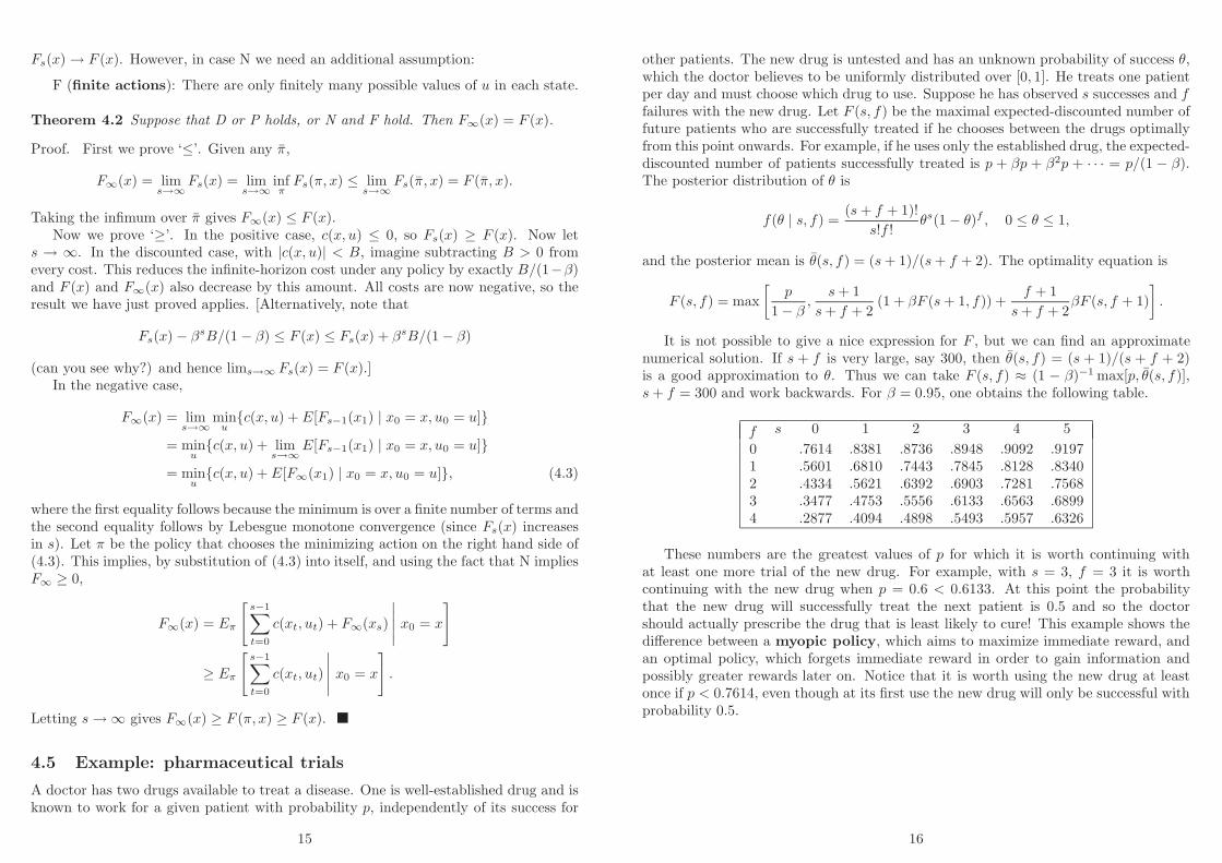
It is not possible to give a nice expression for F , but we can find an approximatenumerical solution. If s + f is very large, say 300, then θ(s, f) = (s + 1)/(s + f + 2)is a good approximation to θ. Thus we can take F (s, f) ≈ (1 − β)−1 max[p, θ(s, f)],s + f = 300 and work backwards. For β = 0.95, one obtains the following table.

s 0 1 2 3 4 5f0 .7614 .8381 .8736 .8948 .9092 .91971 .5601 .6810 .7443 .7845 .8128 .83402 .4334 .5621 .6392 .6903 .7281 .75683 .3477 .4753 .5556 .6133 .6563 .68994 .2877 .4094 .4898 .5493 .5957 .6326

These numbers are the greatest values of p for which it is worth continuing withat least one more trial of the new drug. For example, with s = 3, f = 3 it is worthcontinuing with the new drug when p = 0.6 < 0.6133. At this point the probabilitythat the new drug will successfully treat the next patient is 0.5 and so the doctorshould actually prescribe the drug that is least likely to cure! This example shows thedifference between a myopic policy, which aims to maximize immediate reward, andan optimal policy, which forgets immediate reward in order to gain information andpossibly greater rewards later on. Notice that it is worth using the new drug at leastonce if p < 0.7614, even though at its first use the new drug will only be successful withprobability 0.5.

16

5 Negative Programming

We address the special theory of minimizing positive costs, (noting that the action thatextremizes the right hand side of the optimality equation gives an optimal policy), andstopping problems and their solution.

5.1 Stationary policies

A Markov policy is a policy that specifies the control at time t to be simply a functionof the state and time. In the proof of Theorem 4.1 we used ut = ft(xt) to specify thecontrol at time t. This is a convenient notation for a Markov policy, and we writeπ = (f0, f1, . . . ). If in addition the policy does not depend on time, it is said to be astationary Markov policy, and we write π = (f, f, . . .) = f∞.

5.2 Characterization of the optimal policy

Negative programming concerns minimizing non-negative costs, c(x, u) ≥ 0. The nameoriginates from the equivalent problem of maximizing non-positive rewards, r(x, u) ≤ 0.

The following theorem gives a necessary and sufficient condition for a stationarypolicy to be optimal: namely, it must choose the optimal u on the right hand side ofthe optimality equation. Note that in the statement of this theorem we are requiringthat the infimum over u is attained as a minimum over u.

Theorem 5.1 Suppose D or N holds. Suppose π = f∞ is the stationary Markov policysuch that

c(x, f(x)) + βE[F (x1) | x0 = x, u0 = f(x)]

= minu

[c(x, u) + βE[F (x1) | x0 = x, u0 = u] .

Then F (π, x) = F (x), and π is optimal.

Proof. Suppose this policy is π = f∞. Then by substituting the optimality equationinto itself and using the fact that π specifies the minimizing control at each stage,

F (x) = Eπ

[s−1∑

t=0

βtc(xt, ut)

∣∣∣∣∣x0 = x

]

+ βsEπ [F (xs)|x0 = x] . (5.1)

In case N we can drop the final term on the right hand side of (5.1) (because it isnon-negative) and then let s → ∞; in case D we can let s → ∞ directly, observing thatthis term tends to zero. Either way, we have F (x) ≥ F (π, x).

A corollary is that if assumption F holds then an optimal policy exists. NeitherTheorem 5.1 or this corollary are true for positive programming (c.f., the example inSection 4.1).

17

5.3 Optimal stopping over a finite horizon

One way that the total-expected cost can be finite is if it is possible to enter a statefrom which no further costs are incurred. Suppose u has just two possible values: u = 0(stop), and u = 1 (continue). Suppose there is a termination state, say 0, that is enteredupon choosing the stopping action. Once this state is entered the system stays in thatstate and no further cost is incurred thereafter.

Suppose that stopping is mandatory, in that we must continue for no more that ssteps. The finite-horizon dynamic programming equation is therefore

Fs(x) = min{k(x), c(x) + E[Fs−1(x1) | x0 = x, u0 = 1]} , (5.2)

with F0(x) = k(x), c(0) = 0.Consider the set of states in which it is at least as good to stop now as to continue

one more step and then stop:

S = {x : k(x) ≤ c(x) + E[k(x1) | x0 = x, u0 = 1)]} .

Clearly, it cannot be optimal to stop if x 6∈ S, since in that case it would be strictlybetter to continue one more step and then stop. The following theorem characterisesall finite-horizon optimal policies.

Theorem 5.2 Suppose S is closed (so that once the state enters S it remains in S.)Then an optimal policy for all finite horizons is: stop if and only if x ∈ S.

Proof. The proof is by induction. If the horizon is s = 1, then obviously it is optimalto stop only if x ∈ S. Suppose the theorem is true for a horizon of s − 1. As above, ifx 6∈ S then it is better to continue for more one step and stop rather than stop in statex. If x ∈ S, then the fact that S is closed implies x1 ∈ S and so Fs−1(x1) = k(x1). Butthen (5.2) gives Fs(x) = k(x). So we should stop if s ∈ S.

The optimal policy is known as a one-step look-ahead rule (OSLA).

5.4 Example: optimal parking

A driver is looking for a parking space on the way to his destination. Each parkingspace is free with probability p independently of whether other parking spaces are freeor not. The driver cannot observe whether a parking space is free until he reaches it.If he parks s spaces from the destination, he incurs cost s, s = 0, 1, . . . . If he passesthe destination without having parked the cost is D. Show that an optimal policy is topark in the first free space that is no further than s∗ from the destination, where s∗ isthe greatest integer s such that (Dp + 1)qs ≥ 1.

Solution. When the driver is s spaces from the destination it only matters whetherthe space is available (x = 1) or full (x = 0). The optimality equation gives

Fs(0) = qFs−1(0) + pFs−1(1),

Fs(1) = min

{s, (take available space)qFs−1(0) + pFs−1(1), (ignore available space)

18

where F0(0) = D, F0(1) = 0.Suppose the driver adopts a policy of taking the first free space that is s or closer.

Let the cost under this policy be k(s), where

k(s) = ps + qk(s − 1) ,

with k(0) = qD. The general solution is of the form k(s) = −q/p + s + cqs. So aftersubstituting and using the boundary condition at s = 0, we have

k(s) = − q

p+ s +

(

D +1

p

)

qs+1, s = 0, 1, . . . .

It is better to stop now (at a distance s from the destination) than to go on and takethe first available space if s is in the stopping set

S = {s : s ≤ k(s − 1)} = {s : (Dp + 1)qs ≥ 1} .

This set is closed (since s decreases) and so by Theorem 5.2 this stopping set describesthe optimal policy.

If the driver parks in the first available space past his destination and walk backs,then D = 1 + qD, so D = 1/p and s∗ is the greatest integer such that 2qs ≥ 1.

5.5 Optimal stopping over the infinite horizon

Let us now consider the stopping problem over the infinite-horizon. As above, let Fs(x)be the infimal cost given that we are required to stop by time s. Let F (x) be the infimalcost when all that is required is that we stop eventually. Since less cost can be incurredif we are allowed more time in which to stop, we have

Fs(x) ≥ Fs+1(x) ≥ F (x) .

Thus by monotone convergence Fs(x) tends to a limit, say F∞(x), and F∞(x) ≥ F (x).

Example: we can have F∞ > F

Consider the problem of stopping a symmetric random walk on the integers, wherec(x) = 0, k(x) = exp(−x). The policy of stopping immediately, π, has F (π, x) =exp(−x), and this satisfies the infinite-horizon optimality equation,

F (x) = min{exp(−x), (1/2)F (x + 1) + (1/2)F (x − 1)} .

However, π is not optimal. A symmetric random walk is recurrent, so we may wait untilreaching as large an integer as we like before stopping; hence F (x) = 0. Inductively,one can see that Fs(x) = exp(−x). So F∞(x) > F (x).

(Note: Theorem 4.2 says that F∞ = F , but that is in a setting in which there is noterminal cost and for different definitions of Fs and F than we take here.)

19

Example: Theorem 4.1 is not true for negative programming

Consider the above example, but now suppose one is allowed never to stop. Sincecontinuation costs are 0 the optimal policy for all finite horizons and the infinite horizonis never to stop. So F (x) = 0 and this satisfies the optimality equation above. However,F (π, x) = exp(−x) also satisfies the optimality equation and is the cost incurred bystopping immediately. Thus it is not true (as for positive programming) that a policywhose cost function satisfies the optimality equation is optimal.

The following lemma gives conditions under which the infimal finite-horizon costdoes converge to the infimal infinite-horizon cost.

Lemma 5.3 Suppose all costs are bounded as follows.

(a) K = supx

k(x) < ∞ (b) C = infx

c(x) > 0 . (5.3)

Then Fs(x) → F (x) as s → ∞.

Proof. (*starred*) Suppose π is an optimal policy for the infinite horizon problem andstops at the random time τ . Then its cost is at least (s + 1)CP (τ > s). However, sinceit would be possible to stop at time 0 the cost is also no more than K, so

(s + 1)CP (τ > s) ≤ F (x) ≤ K .

In the s-horizon problem we could follow π, but stop at time s if τ > s. This implies

F (x) ≤ Fs(x) ≤ F (x) + KP (τ > s) ≤ F (x) +K2

(s + 1)C.

By letting s → ∞, we have F∞(x) = F (x).

Note that the problem posed here is identical to one in which we pay K at the startand receive a terminal reward r(x) = K − k(x).

Theorem 5.4 Suppose S is closed and (5.3) holds. Then an optimal policy for theinfinite horizon is: stop if and only if x ∈ S.

Proof. By Theorem 5.2 we have for all finite s,

Fs(x)= k(x) x ∈ S ,< k(x) x 6∈ S .

Lemma 5.3 gives F (x) = F∞(x).

20

6 Average-cost Programming

We address the infinite-horizon average-cost case, the optimality equation for this caseand the policy improvement algorithm.

6.1 Average-cost optimization

It can happen that the undiscounted expected total cost is infinite, but the accumulationof cost per unit time is finite. Suppose that for a stationary Markov policy π, thefollowing limit exists:

λ(π, x) = limt→∞

1

tEπ

[t−1∑

s=0

c(xs, us)

∣∣∣∣∣x0 = x

]

.

It is reasonable to expect that there is a well-defined notion of an optimal average-costfunction, λ(x) = infπ λ(π, x), and that under appropriate assumptions, λ(x) = λ shouldnot depend on x. Moreover, one would expect

Fs(x) = sλ + φ(x) + ǫ(s, x) ,

where ǫ(s, x) → 0 as s → ∞. Here φ(x) + ǫ(s, x) reflects a transient due to the initialstate. Suppose that the state space and action space are finite. From the optimalityequation for the finite horizon problem we have

Fs(x) = minu

{c(x, u) + E[Fs−1(x1) | x0 = x, u0 = u]} . (6.1)

So by substituting Fs(x) ∼ sλ + φ(x) into (6.1), we obtain

sλ + φ(x) ∼ minu

{c(x, u) + E[(s − 1)λ + φ(x1) | x0 = x, u0 = u]}

which suggests, what it is in fact, the average-cost optimality equation:

λ + φ(x) = minu

{c(x, u) + E[φ(x1) | x0 = x, u0 = u]} . (6.2)

Theorem 6.1 Let λ denote the minimal average-cost. Suppose there exists a constantλ′ and bounded function φ such that for all x and u,

λ′ + φ(x) ≤ c(x, u) + E[φ(x1) | x0 = x, u0 = u] . (6.3)

Then λ′ ≤ λ. This also holds when ≤ is replaced by ≥ and the hypothesis is weakenedto: for each x there exists a u such that (6.3) holds when ≤ is replaced by ≥.

Proof. Suppose u is chosen by some policy π. By repeated substitution of (6.3) intoitself we have

φ(x) ≤ −tλ′ + Eπ

[t−1∑

s=0

c(xs, us)

∣∣∣∣∣x0 = x

]

+ Eπ [φ(xt) | x0 = x]

21

Divide this by t and let t → ∞ to obtain

0 ≤ −λ′ + limt→∞

1

tEπ

[t−1∑

s=0

c(xs, us)

∣∣∣∣∣x0 = x

]

,

where the final term on the right hand side is simply the average-cost under policy π.Minimizing the right hand side over π gives the result. The claim for ≤ replaced by ≥is proved similarly.

Theorem 6.2 Suppose there exists a constant λ and bounded function φ satisfying(6.2). Then λ is the minimal average-cost and the optimal stationary policy is the onethat chooses the optimizing u on the right hand side of (6.2).

Proof. Equation (6.2) implies that (6.3) holds with equality when one takes π to be thestationary policy that chooses the optimizing u on the right hand side of (6.2). Thus πis optimal and λ is the minimal average-cost.

The average-cost optimal policy is found simply by looking for a bounded solutionto (6.2). Notice that if φ is a solution of (6.2) then so is φ+(a constant), because the(a constant) will cancel from both sides of (6.2). Thus φ is undetermined up to anadditive constant. In searching for a solution to (6.2) we can therefore pick any state,say x, and arbitrarily take φ(x) = 0.

6.2 Example: admission control at a queue

Each day a consultant is presented with the opportunity to take on a new job. Thejobs are independently distributed over n possible types and on a given day the offeredtype is i with probability ai, i = 1, . . . , n. Jobs of type i pay Ri upon completion.Once he has accepted a job he may accept no other job until that job is complete. Theprobability that a job of type i takes k days is (1 − pi)

k−1pi, k = 1, 2, . . . . Which jobsshould the consultant accept?

Solution. Let 0 and i denote the states in which he is free to accept a job, and inwhich he is engaged upon a job of type i, respectively. Then (6.2) is

λ + φ(0) =

n∑

i=1

ai max[φ(0), φ(i)],

λ + φ(i) = (1 − pi)φ(i) + pi[Ri + φ(0)], i = 1, . . . , n .

Taking φ(0) = 0, these have solution φ(i) = Ri − λ/pi, and hence

λ =

n∑

i=1

ai max[0, Ri − λ/pi] .

The left hand side is increasing in λ and the right hand side is decreasing λ. Hencethere is a root, say λ∗, and this is the maximal average-reward. The optimal policytakes the form: accept only jobs for which piRi ≥ λ∗.

22

6.3 Value iteration bounds

Value iteration in the average-cost case is based upon the idea that Fs(x) − Fs−1(x)approximates the minimal average-cost for large s.

Theorem 6.3 Define

ms = minx

{Fs(x) − Fs−1(x)} , Ms = maxx

{Fs(x) − Fs−1(x)} . (6.4)

Then ms ≤ λ ≤ Ms, where λ is the minimal average-cost.

Proof. (*starred*) Suppose that the first step of a s-horizon optimal policy followsMarkov plan f . Then

Fs(x) = Fs−1(x) + [Fs(x) − Fs−1(x)] = c(x, f(x)) + E[Fs−1(x1) | x0 = x, u0 = f(x)] .

HenceFs−1(x) + ms ≤ c(x, u) + E[Fs−1(x1) | x0 = x, u0 = u] ,

for all x, u. Applying Theorem 6.1 with φ = Fs−1 and λ′ = ms, implies ms ≤ λ. Thebound λ ≤ Ms is established in a similar way.

This justifies the following value iteration algorithm. At termination the algo-rithm provides a stationary policy that is within ǫ × 100% of optimal.

(0) Set F0(x) = 0, s = 1.(1) Compute Fs from

Fs(x) = minu

{c(x, u) + E[Fs−1(x1) | x0 = x, u0 = u]} .

(2) Compute ms and Ms from (6.4). Stop if Ms − ms ≤ ǫms. Otherwise set s := s + 1and goto step (1).

6.4 Policy improvement

Policy improvement is an effective method of improving stationary policies.

Policy improvement in the average-cost case.

In the average-cost case a policy improvement algorithm can be based on the followingobservations. Suppose that for a policy π = f∞, we have that λ, φ is a solution to

λ + φ(x) = c(x, f(x0)) + E[φ(x1) | x0 = x, u0 = f(x0)] ,

and suppose for some policy π1 = f∞1 ,

λ + φ(x) ≥ c(x, f1(x0)) + E[φ(x1) | x0 = x, u0 = f1(x0)] , (6.5)

23

with strict inequality for some x. Then following the lines of proof in Theorem 6.1

limt→∞

1

tEπ

[t−1∑

s=0

c(xs, us)

∣∣∣∣∣x0 = x

]

= λ ≥ limt→∞

1

tEπ1

[t−1∑

s=0

c(xs, us)

∣∣∣∣∣x0 = x

]

.

If there is no π1 for which (6.5) holds then π satisfies (6.2) and is optimal. This justifiesthe following policy improvement algorithm

(0) Choose an arbitrary stationary policy π0. Set s = 1.(1) For a given stationary policy πs−1 = f∞

s−1 determine φ, λ to solve

λ + φ(x) = c(x, fs−1(x)) + E[φ(x1) | x0 = x, u0 = fs−1(x)] .

This gives a set of linear equations, and so is intrinsically easier to solve than (6.2).(2) Now determine the policy πs = f∞

s from

c(x, fs(x)) + E[φ(x1) | x0 = x, u0 = fs(x)]

= minu

{c(x, u) + E[φ(x1) | x0 = x, u0 = u]} ,

taking fs(x) = fs−1(x) whenever this is possible. By applications of Theorem 6.1,this yields a strict improvement whenever possible. If πs = πs−1 then the algorithmterminates and πs−1 is optimal. Otherwise, return to step (1) with s := s + 1.

If both the action and state spaces are finite then there are only a finite numberof possible stationary policies and so the policy improvement algorithm will find anoptimal stationary policy in finitely many iterations. By contrast, the value iterationalgorithm can only obtain more and more accurate approximations of λ∗.

Policy improvement in the discounted-cost case.

In the case of strict discounting, the following theorem plays the role of Theorem 6.1.The proof is similar, by repeated substitution of (6.6) into itself.

Theorem 6.4 Suppose there exists a bounded function G such that for all x and u,

G(x) ≤ c(x, u) + βE[G(x1) | x0 = x, u0 = u]. (6.6)

Then G ≤ F , where F is the minimal discounted-cost function. This also holds when≤ is replaced by ≥ and the hypothesis is weakened to: for each x there exists a u suchthat (6.6) holds when ≤ is replaced by ≥.

The policy improvement algorithm is similar. E.g., step (1) becomes

(1) For a given stationary policy πs−1 = f∞s−1 determine G to solve

G(x) = c(x, fs−1(x)) + βE[G(x1) | x0 = x, u0 = fs−1(x)] .

24

7 LQ Models

We present the LQ regulation model in discrete and continuous time, the Riccati equa-tion, its validity in the model with additive white noise.

7.1 The LQ regulation model

The elements needed to define a control optimization problem are specification of (i)the dynamics of the process, (ii) which quantities are observable at a given time, and(iii) an optimization criterion.

In the LQG model the plant equation and observation relations are linear, thecost is quadratic, and the noise is Gaussian (jointly normal). The LQG model is im-portant because it has a complete theory and introduces some key concepts, such ascontrollability, observability and the certainty-equivalence principle.

Begin with a model in which the state xt is fully observable and there is no noise.The plant equation of the time-homogeneous [A, B, · ] system has the linear form

xt = Axt−1 + But−1 , (7.1)

where xt ∈ Rn, ut ∈ R

m, A is n × n and B is n × m. The cost function is

C =

h−1∑

t=0

c(xt, ut) + Ch(xh) , (7.2)

with one-step and terminal costs

c(x, u) = x⊤Rx + u⊤Sx + x⊤S⊤u + u⊤Qu =

[xu

]⊤ [R S⊤

S Q

] [xu

]

, (7.3)

Ch(x) = x⊤Πhx . (7.4)

All quadratic forms are non-negative definite, and Q is positive definite. There is noloss of generality in assuming that R, Q and Πh are symmetric. This is a model forregulation of (x, u) to the point (0, 0) (i.e., steering to a critical value).

To solve the optimality equation we shall need the following lemma.

Lemma 7.1 Suppose x, u are vectors. Consider a quadratic form

(xu

)⊤ (Πxx Πxu

Πux Πuu

) (xu

)

.

Assume it is symmetric and Πuu > 0, i.e., positive definite. Then the minimum withrespect to u is achieved at

u = −Π−1uuΠuxx,

and is equal tox⊤

[Πxx − ΠxuΠ−1

uu Πux

]x.

25

Proof. Suppose the quadratic form is minimized at u. Then

(x

u + h

)⊤ (Πxx Πxu

Πux Πuu

) (x

u + h

)

= x⊤Πxxx + 2x⊤Πxuu + 2h⊤Πuxx + 2h⊤Πuuu︸ ︷︷ ︸

+u⊤Πuuu + h⊤Πuuh .

To be stationary at u, the underbraced linear term in h⊤ must be zero, so

u = −Π−1uuΠuxx ,

and the optimal value is x⊤[Πxx − ΠxuΠ−1

uu Πux

]x.

Theorem 7.2 Assume the structure of (7.1)–(7.4). Then the value function has thequadratic form

F (x, t) = x⊤Πtx , t < h , (7.5)

and the optimal control has the linear form

ut = Ktxt , t < h .

The time-dependent matrix Πt satisfies the Riccati equation

Πt = fΠt+1 , t < h , (7.6)

where f is an operator having the action

fΠ = R + A⊤ΠA − (S⊤ + A⊤ΠB)(Q + B⊤ΠB)−1(S + B⊤ΠA) , (7.7)

and Πh has the value prescribed in (7.4). The m × n matrix Kt is given by

Kt = −(Q + B⊤Πt+1B)−1(S + B⊤Πt+1A) , t < h .

Proof. Assertion (7.5) is true at time h. Assume it is true at time t + 1. Then

F (x, t) = infu

[c(x, u) + (Ax + Bu)⊤Πt+1(Ax + Bu)

]

= infu

[(xu

)⊤ (R + A⊤Πt+1A S⊤ + A⊤Πt+1BS + B⊤Πt+1A Q + B⊤Πt+1B

) (xu

)]

By Lemma 7.1 the minimum is achieved by u = Ktx, and the form of f comes fromthis also.

26

7.2 The Riccati recursion

The backward recursion (7.6)–(7.7) is called the Riccati equation. Note that

(i) S can be normalized to zero by choosing a new control u∗ = u+Q−1Sx, and settingA∗ = A − BQ−1S, R∗ = R − S⊤Q−1S.

(ii) The optimally controlled process obeys xt+1 = Γtxt. Here Γt is called the gainmatrix and is given by

Γt = A + BKt = A − B(Q + B⊤Πt+1B)−1(S + B⊤Πt+1A) .

(iii) An equivalent expression for the Riccati equation is

fΠ = infK

[R + K⊤S + S⊤K + K⊤QK + (A + BK)⊤Π(A + BK)

].

(iv) We might have carried out exactly the same analysis for a time-heterogeneousmodel, in which the matrices A, B, Q, R, S are replaced by At, Bt, Qt, Rt, St.

(v) We do not give details, but comment that it is possible to analyse models in which

xt+1 = Axt + But + αt ,

for a known sequence of disturbances {αt}, or in which the cost function is

c(x, u) =

[x − xt

u − ut

]⊤ [R S⊤

S Q

] [x − xt

u − ut

]

.

so that the aim is to track a sequence of values (xt, ut), t = 0, . . . , h − 1.

7.3 White noise disturbances

Suppose the plant equation (7.1) is now

xt+1 = Axt + But + ǫt,

where ǫt ∈ Rn is vector white noise, defined by the properties Eǫ = 0, Eǫtǫ

⊤t = N

and Eǫtǫ⊤s = 0, t 6= s. The DP equation is then

F (x, t) = infu

[

c(x, u) + Eǫ[(F (Ax + Bu + ǫ, t + 1)]

]

.

By definition F (x, h) = x⊤Πhx. Try a solution F (x, t) = x⊤Πtx + γt. This holds fort = h. Suppose it is true for t + 1, then

F (x, t) = infu

[c(x, u) + E(Ax + Bu + ǫ)⊤Πt+1(Ax + Bu + ǫ) + γt+1

]

= infu

[c(x, u) + E(Ax + Bu)⊤Πt+1(Ax + Bu)

]

+ 2E[ǫ⊤(Ax + Bu)

]+ E

[ǫ⊤Πt+1ǫ

]+ γt+1

= infu

[· · · ] + 0 + tr(NΠt+1) + γt+1 .

27

Here we use the fact that

E[ǫ⊤Πǫ

]= E

∑

ij

ǫiΠijǫj

= E

∑

ij

ǫjǫiΠij

=∑

ij

NjiΠij = tr(NΠ) .

Thus (i) Πt follows the same Riccati equation as before, (ii) the optimal control isut = Ktxt, and (iii)

F (x, t) = x⊤Πtx + γt = x⊤Πtx +

h∑

j=t+1

tr(NΠj) .

The final term can be viewed as the cost of correcting future noise. In the infinitehorizon limit of Πt → Π as t → ∞, we incur an average cost per unit time of tr(NΠ),and a transient cost of x⊤Πx that is due to correcting the initial x.

7.4 LQ regulation in continuous-time

In continuous-time we take x = Ax + Bu and

C =

∫ h

0

(xu

)⊤ (R S⊤

S Q

) (xu

)

dt + (x⊤Πx)h .

We can obtain the continuous-time solution from the discrete time solution by movingforward in time in increments of ∆. Make the following replacements.

xt+1 → xt+∆, A → I + A∆, B → B∆, R, S, Q → R∆, S∆, Q∆ .

Then as before, F (x, t) = x⊤Πx, where Π obeys the Riccati equation

∂Π

∂t+ R + A⊤Π + ΠA − (S⊤ + ΠB)Q−1(S + B⊤Π) = 0 .

This is simpler than the discrete time version. The optimal control is

u(t) = K(t)x(t)

where

K(t) = −Q−1(S + B⊤Π) .

The optimally controlled plant equation is x = Γ(t)x, where

Γ(t) = A + BK = A − BQ−1(S + B⊤Π) .

28

8 Controllability

We define and give conditions for controllability in discrete and continuous time.

8.1 Controllability

Consider the [A, B, · ] system with plant equation xt+1 = Axt + ut. The controlla-bility question is: can we bring x to an arbitrary prescribed value by some u-sequence?

Definition 8.1 The system is r-controllable if one can bring it from an arbitraryprescribed x0 to an arbitrary prescribed xr by some u-sequence u0, u1, . . . , ur−1. Asystem of dimension n is said to be controllable if it is r-controllable for some r

Example. If B is square and non-singular then the system is 1-controllable, for

x1 = Ax0 + Bu0 where u0 = B−1(x1 − Ax0) .

Example. Consider the case, (n = 2, m = 1),

xt =

(a11 0a21 a22

)

xt−1 +

(10

)

ut−1.

This system is not 1-controllable. But

x2 − A2x0 = Bu1 + ABu0 =

(1 a11

0 a21

) (u1

u0

)

.

So it is 2-controllable if and only if a21 6= 0.

More generally, by substituting the plant equation into itself, we see that we mustfind u0, u1, . . . , ur−1 to satisfy

∆ = xr − Arx0 = Bur−1 + ABur−2 + · · · + Ar−1Bu0, (8.1)

for arbitrary ∆. In providing conditions for controllability we shall need to make useof the following theorem.

Theorem 8.2 (The Cayley-Hamilton theorem) Any n × n matrix A satisfies itsown characteristic equation. So that if

det(λI − A) =n∑

j=0

ajλn−j

thenn∑

j=0

ajAn−j = 0. (8.2)

29

The implication is that I, A, A2, . . . , An−1 contains basis for Ar, r = 0, 1, . . . . Proof.(*starred*) Define

Φ(z) =

∞∑

j=0

(Az)j = (I − Az)−1 =adj(I − Az)

det(I − Az).

Then

det(I − Az)Φ(z) =

n∑

j=0

ajzjΦ(z) = adj(I − Az),

which implies (8.2) since the coefficient of zn must be zero.

We are now in a position to characterise controllability.

Theorem 8.3 (i) The system [A, B, · ] is r-controllable if and only if the matrix

Mr =[B AB A2B · · · Ar−1B

]

has rank n, or (ii) equivalently, if and only if the n × n matrix

MrM⊤r =

r−1∑

j=0

Aj(BB⊤)(A⊤)j

is nonsingular (or, equivalently, positive definite.) (iii) If the system is r-controllablethen it is s-controllable for s ≥ min(n, r), and (iv) a control transferring x0 to xr with

minimal cost∑r−1

t=0 u⊤t ut is

ut = B⊤(A⊤)r−t−1(MrM⊤r )−1(xr − Arx0), t = 0, . . . , r − 1.

Proof. (i) The system (8.1) has a solution for arbitrary ∆ if and only if Mr has rankn. (ii) MrM

⊤r is singular if and only if there exists w such that MrM

⊤r w = 0, and

MrM⊤r w = 0 ⇐⇒ w⊤MrM

⊤r w = 0 ⇐⇒ M⊤

r w = 0.

(iii) The rank of Mr is non-decreasing in r, so if it is r-controllable, then it is s-controllable for s ≥ r. But the rank is constant for r ≥ n by the Cayley-Hamiltontheorem. (iv) Consider the Lagrangian

r−1∑

t=0

u⊤t ut + λ⊤(∆ −

r−1∑

t=0

Ar−t−1But),

givingut = 1

2B⊤(A⊤)r−t−1λ.

Now we can determine λ from (8.1).

30

8.2 Controllability in continuous-time

Theorem 8.4 (i) The n dimensional system [A, B, · ] is controllable if and only ifthe matrix Mn has rank n, or (ii) equivalently, if and only if

G(t) =

∫ t

0

eAsBB⊤eA⊤s ds,

is positive definite for all t > 0. (iii) If the system is controllable then a control that

achieves the transfer from x(0) to x(t) with minimal control cost∫ t

0u⊤

s usds is

u(s) = B⊤eA⊤(t−s)G(t)−1(x(t) − eAtx(0)).

Note that there is now no notion of r-controllability. However, G(t) ↓ 0 as t ↓ 0, sothe transfer becomes more difficult and costly as t ↓ 0.

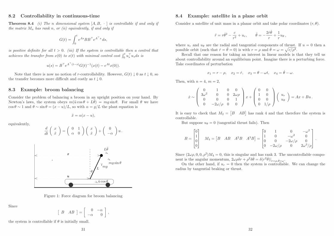
8.3 Example: broom balancing

Consider the problem of balancing a broom in an upright position on your hand. ByNewton’s laws, the system obeys m(u cos θ + Lθ) = mg sin θ. For small θ we havecos θ ∼ 1 and θ ∼ sin θ = (x − u)/L, so with α = g/L the plant equation is

x = α(x − u),

equivalently,d

dt

(xx

)

=

(0 1α 0

) (xx

)

+

(0−α

)

u .

mg

Lθ

xx

θ

uu

L

u cos θ

mg sin θ

Figure 1: Force diagram for broom balancing

Since[

B AB]

=

[0 −α

−α 0

]

,

the system is controllable if θ is initially small.

31

8.4 Example: satellite in a plane orbit

Consider a satellite of unit mass in a planar orbit and take polar coordinates (r, θ).

r = rθ2 − c

r2+ ur, θ = −2rθ

r+

1

ruθ ,

where ur and uθ are the radial and tangential components of thrust. If u = 0 then apossible orbit (such that r = θ = 0) is with r = ρ and θ = ω =

√

c/ρ3.Recall that one reason for taking an interest in linear models is that they tell us

about controllability around an equilibrium point. Imagine there is a perturbing force.Take coordinates of perturbation

x1 = r − ρ, x2 = r, x3 = θ − ωt, x4 = θ − ω.

Then, with n = 4, m = 2,

x ∼

0 1 0 03ω2 0 0 2ωρ0 0 0 10 −2ω/ρ 0 0

x +

0 01 00 00 1/ρ

(ur

uθ

)

= Ax + Bu .

It is easy to check that M2 =[B AB

]has rank 4 and that therefore the system is

controllable.But suppose uθ = 0 (tangential thrust fails). Then

B =

0100

M4 =[B AB A2B A3B

]=

0 1 0 −ω2

1 0 −ω2 00 0 −2ω/ρ 00 −2ω/ρ 0 2ω3/ρ

.

Since (2ωρ, 0, 0, ρ2)M4 = 0, this is singular and has rank 3. The uncontrollable compo-nent is the angular momentum, 2ωρδr + ρ2δθ = δ(r2θ)|r=ρ,θ=ω.

On the other hand, if ur = 0 then the system is controllable. We can change theradius by tangential braking or thrust.

32

9 Infinite Horizon Limits

We define stabilizability and discuss the LQ regulation problem over an infinite horizon.

9.1 Linearization of nonlinear models

Linear models are important because they arise naturally via the linearization of non-linear models. Consider the state-structured nonlinear model:

x = a(x, u).

Suppose x, u are perturbed from an equilibrium (x, u) where a(x, u) = 0. Let x′ = x− xand u′ = u − u and immediately drop the primes. The linearized version is

x = Ax + Bu

where

A =∂a

∂x

∣∣∣∣(x,u)

, B =∂a

∂u

∣∣∣∣(x,u)

.

If x, u is to be a stable equilibrium point then we must be able to choose a control thatcan stabilise the system in the neighbourhood of (x, u).

9.2 Stabilizability

Suppose we apply the stationary control u = Kx so that x = Ax + Bu = (A + BK)x.So with Γ = A + BK, we have

x = Γx, xt = eΓtx0, where eΓt =

∞∑

j=0

(Γt)j/j!

Similarly, in discrete-time, we have can take the stationary control, ut = Kxt, sothat xt = Axt−1 + But−1 = (A + BK)xt−1. Now xt = Γtx0.

We are interested in choosing Γ so that xt → 0 and t → ∞.

Definition 9.1Γ is a stability matrix in the continuous-time sense if all its eigenvalues have

negative real part, and hence xt → 0 as t → ∞.

Γ is a stability matrix in the discrete-time sense if all its eigenvalues of lie strictlyinside the unit disc in the complex plane, |z| = 1, and hence xt → 0 as t → ∞.

The [A, B] system is said to stabilizable if there exists a K such that A + BK isa stability matrix.

Note that ut = Kxt is linear and Markov. In seeking controls such that xt → 0 itis sufficient to consider only controls of this type since, as we see below, such controlsarise as optimal controls for the infinite-horizon LQ regulation problem.

33

9.3 Example: pendulum

Consider a pendulum of length L, unit mass bob and angle θ to the vertical. Supposewe wish to stabilise θ to zero by application of a force u. Then

θ = −(g/L) sin θ + u.

We change the state variable to x = (θ, θ) and write

d

dt

(θ

θ

)

=

(

θ−(g/L) sin θ + u

)

∼(

θ−(g/L)θ

)

+

(0u

)

=

(0 1

−(g/L) 0

) (θ

θ

)

+

(01

)

u.

Suppose we try to stabilise with a control u = −Kθ = −Kx1. Then

A + BK =

(0 1

−(g/L)− K 0

)

and this has eigenvalues ±√

−(g/L)− K. So either −(g/L)−K > 0 and one eigenvaluehas a positive real part, in which case there is in fact instability, or −(g/L) − K < 0and eigenvalues are purely imaginary, which means we will in general have oscillations.So successful stabilization must be a function of θ as well, (and this would come out ofsolution to the LQ regulation problem.)

9.4 Infinite-horizon LQ regulation

Consider the time-homogeneous case and write the finite-horizon cost in terms of timeto go s. The terminal cost, when s = 0, is denoted F0(x) = x⊤Π0x. In all that followswe take S = 0, without loss of generality.

Lemma 9.2 Suppose Π0 = 0, R ≥ 0, Q ≥ 0 and [A, B, · ] is controllable or stabiliz-able. Then {Πs} has a finite limit Π.

Proof. Costs are non-negative, so Fs(x) is non-decreasing in s. Now Fs(x) = x⊤Πsx.Thus x⊤Πsx is non-decreasing in s for every x. To show that x⊤Πsx is bounded we useone of two arguments.

If the system is controllable then x⊤Πsx is bounded because there is a policy which,for any x0 = x, will bring the state to zero in at most n steps and at finite cost and canthen hold it at zero with zero cost thereafter.

34

If the system is stabilizable then there is a K such that Γ = A + BK is a stabilitymatrix and using ut = Kxt, we have

Fs(x) ≤ x⊤

[∞∑

t=0

(Γ⊤)t(R + K⊤QK)Γt

]

x < ∞.

Hence in either case we have an upper bound and so x⊤Πsx tends to a limit forevery x. By considering x = ej, the vector with a unit in the jth place and zeroselsewhere, we conclude that the jth element on the diagonal of Πs converges. Thentaking x = ej + ek it follows that the off diagonal elements of Πs also converge.

Both value iteration and policy improvement are effective ways to compute thesolution to an infinite-horizon LQ regulation problem. Policy improvement goes alongthe lines developed in Lecture 6.

The following theorem establishes the efficacy of value iteration. It is similar toTheorem 4.2 which established the same fact for D, N and P programming. The LQregulation problem is a negative programming problem, however we cannot apply The-orem 4.2, because in general the terminal cost of x⊤Π0x is not zero.

Theorem 9.3 Suppose that R > 0, Q > 0 and the system [A, B, · ] is controllable.Then (i) The equilibrium Riccati equation

Π = fΠ (9.1)

has a unique non-negative definite solution Π. (ii) For any finite non-negative definiteΠ0 the sequence {Πs} converges to Π. (iii) The gain matrix Γ corresponding to Π is astability matrix.

Proof. (*starred*) Define Π as the limit of the sequence f (s)0. By the previous lemmawe know that this limit exists and that it satisfies (9.1).

Consider ut = Kxt and xt+1 = (A + BK)xt = Γxt = Γtx0, for arbitrary x0, whereK = −(Q + B⊤ΠB)−1B⊤ΠA and Γ = A + BK. We can write (9.1) as

Π = R + K⊤QK + Γ⊤ΠΓ. (9.2)

and hencex⊤

t Πxt = x⊤t (R + K⊤QK)xt + x⊤

t+1Πxt+1 ≥ x⊤t+1Πxt+1.

Thus x⊤t Πxt decreases and, being bounded below by zero, it tends to a limit. Thus

x⊤t (R+K⊤QK)xt tends to 0. Since R+K⊤QK is positive definite this implies xt → 0,

which implies (iii). Hence for arbitrary finite non-negative definite Π0,

Πs = f (s)Π0 ≥ f (s)0 → Π. (9.3)

However, if we choose the fixed policy ut = Kxt then it follows that

Πs ≤ f (s)0 + (Γ⊤)sΠ0Γs → Π. (9.4)

Thus (9.3) and (9.4) imply (ii).Finally, if non-negative definite Π also satisfies (9.1) then Π = f (s)Π → Π, whence

(i) follows.

35

9.5 The [A, B, C] system

The notion of controllability rested on the assumption that the initial value of thestate was known. If, however, one must rely upon imperfect observations, then thequestion arises whether the value of state (either in the past or in the present) can bedetermined from these observations. The discrete-time system [A, B, C] is defined bythe plant equation and observation relation

xt = Axt−1 + But−1,

yt = Cxt−1.

Here y ∈ Rr is observed, but x is not. We suppose C is r × n. The observability

question is whether or not we can infer x0 from the observations y1, y2, . . .. The notionof observability stands in dual relation to that of controllability; a duality that indeedpersists throughout the subject.

36

10 Observability

We present observability and the LQG model with process and observation noise.

10.1 Observability

The previous lecture introduced the [A, B, C] system,

xt = Axt−1 + But−1, (10.1)

yt = Cxt−1. (10.2)

y ∈ Rk is observed, but x is not. C is k × n. The observability question is: can we

infer x at a prescribed time by subsequent y values?

Definition 10.1 A system is said to be r-observable if x0 can be inferred from knowl-edge of the subsequent observations y1, . . . , yr and relevant control values u0, . . . , ur−2

for any initial x0. A system of dimension n is said to be observable if it is r-observablefor some r.

From (10.1) and (10.2) we can determine yt in terms of x0 and subsequent controls:

xt = Atx0 +

t−1∑

s=0

AsBut−s−1,

yt = Cxt−1 = C

[

At−1x0 +

t−2∑

s=0

AsBut−s−2

]

.

Thus, if we define the ‘reduced observation’

yt = yt − C

[t−2∑

s=0

AsBut−s−2

]

,

then x0 is to be determined from the system of equations

yt = CAt−1x0, 1 ≤ t ≤ r. (10.3)

By hypothesis, these equations are mutually consistent, and so have a solution; thequestion is whether this solution is unique. This is the reverse of the situation forcontrollability, when the question was whether the equation for u had a solution at all,unique or not. Note that an implication of the system definition is that the property ofobservability depends only on the matrices A and C; not upon B at all.

Theorem 10.2 (i) The system [A, · , C] is r-observable if and only if the matrix

Nr =

CCACA2

...CAr−1

37

has rank n, or (ii) equivalently, if and only if the n × n matrix

N⊤r Nr =

r−1∑

j=0

(A⊤)jC⊤CAj

is nonsingular. (iii) If the system is r-observable then it is s-observable for s ≥min(n, r), and (iv) the determination of x0 can be expressed

x0 = (N⊤r Nr)

−1r∑

j=1

(A⊤)j−1C⊤yj. (10.4)

Proof. If the system has a solution for x0 (which is so by hypothesis) then this solutionmust is unique if and only if the matrix Nr has rank n, whence assertion (i). Assertion(iii) follows from (i). The equivalence of conditions (i) and (ii) can be verified directlyas in the case of controllability.

If we define the deviation ηt = yt − CAt−1x0 then the equation amounts to ηt = 0,1 ≤ t ≤ r. If these equations were not consistent we could still define a ‘least-squares’solution to them by minimizing any positive-definite quadratic form in these deviationswith respect to x0. In particular, we could minimize

∑r−1t=0 η⊤

t ηt. This minimizationgives (10.4). If equations (10.3) indeed have a solution (i.e., are mutually consistent,as we suppose) and this is unique then expression (10.4) must equal this solution; theactual value of x0. The criterion for uniqueness of the least-squares solution is thatN⊤

r Nr should be nonsingular, which is also condition (ii).

Note that we have again found it helpful to bring in an optimization criterion inproving (iv); this time, not so much to construct one definite solution out of many, butrather to construct a ‘best-fit’ solution where an exact solution might not have existed.This approach lies close to the statistical approach necessary when observations arecorrupted by noise.

10.2 Observability in continuous-time

Theorem 10.3 (i) The n-dimensional continuous-time system [A, · , C] is observableif and only if the matrix Nn has rank n, or (ii) equivalently, if and only if

H(t) =

∫ t

0

eA⊤sC⊤CeAs ds

is positive definite for all t > 0. (iii) If the system is observable then the determinationof x(0) can be written

x(0) = H(t)−1

∫ t

0

eA⊤sC⊤y(s) ds,

where

y(t) = y(t) −∫ t

0

CAt−sBu(s) ds.

38

10.3 Examples

Example. Observation of populationConsider two populations whose sizes are changing according to the equations

x1 = λ1x1, x2 = λ2x2.

Suppose we observe x1 + x2, so

A =

(λ1 00 λ2

)

, C =(

1 1), N2 =

(1 1λ1 λ2

)

.

and so the individual populations are observable if λ1 6= λ2.

Example. Radioactive decaySuppose j = 1, 2, 3 and decay is from 1 to 2 at rate α, from 1 to 3 at rate β and from2 to 3 at rate γ. We observe only the accumulation in state 3. Then x = Ax, where

A =

−α − β 0 0α −γ 0β γ 0

, C =(

0 0 1),

N3 =

CCACA2

=

0 0 1β γ 0

αγ − β(α + β) −γ2 0

.

The determinant equals γ(α + β)(γ − β), so we require γ > 0, α + β > 0, β 6= γ for anonzero determinant and observability.

Example. SatelliteRecall the linearised equation x = Ax, for perturbations of the orbit of a satellite, (heretaking ρ = 1), where

x1

x2

x3

x4

=

r − ρr

θ − ωt

θ − ω

A =

0 1 0 03ω2 0 0 2ω0 0 0 10 −2ω 0 0

.

By taking C =[0 0 1 0

]we see that we can see that system is observable on

the basis of angle measurements alone but, not observable for C =[1 0 0 0

], i.e.,

on the basis of radius movements alone.

N4 =

0 0 1 00 0 0 10 −2ω 0 0

−6ω3 0 0 −4ω2

N4 =

1 0 0 00 1 0 0

3ω2 0 0 2ω0 −ω2 0 0

39

10.4 Imperfect state observation with noise

The full LQG model, whose description has been deferred until now, assumes lineardynamics, quadratic costs and Gaussian noise. Imperfect observation is the most im-portant point. The model is

xt = Axt−1 + But−1 + ǫt, (10.5)

yt = Cxt−1 + ηt, (10.6)

where ǫt is process noise, yt is the observation at time t and ηt is the observation noise.The state observations are degraded in that we observe only Cxt−1. Assume

cov

(ǫη

)

= E

(ǫη

) (ǫη

)⊤

=

(N LL⊤ M

)

and that x0 ∼ N(x0, V0). Let Wt = (Yt, Ut−1) = (y1, . . . , yt; u0, . . . , ut−1) denote theobserved history up to time t. Of course we assume that t, A, B, C, N , L, M , x0 andV0 are also known; Wt denotes what might be different if the process were rerun. Inthe next lecture we turn to the question of estimating x from y.

We consider the issues of state estimation and optimal control and shall show:

(i) xt can be calculated recursively from the Kalman filter (a linear operator):

xt = Axt−1 + But−1 + Ht(yt − Cxt−1),

which is like the plant equation except that the noise is given by an innovationprocess, yt = yt − Cxy, rather than the white noise.

(ii) If with full information (i.e., yt = xt) the optimal control is ut = Ktxt, thenwithout full information the optimal control is ut = Ktxt, where xt is the bestlinear least squares estimate of xt based on the information (Yt, Ut−1) at time t.

Many of the ideas we encounter in this analysis are unrelated to the special statestructure and are therefore worth noting as general observations about control withimperfect information.

40

11 Kalman Filtering and Certainty Equivalence

We presents the important concepts of the Kalman filter, certainty-equivalence and theseparation principle.

11.1 Preliminaries

Lemma 11.1 Suppose x and y are jointly normal with zero means and covariancematrix

cov

[xy

]

=

[Vxx Vxy

Vyx Vyy

]

.

Then the distribution of x conditional on y is Gaussian, with

E(x | y) = VxyV −1yy y , (11.1)

andcov(x | y) = Vxx − VxyV −1

yy Vyx . (11.2)

Proof. Both y and x−VxyV −1yy y are linear functions of x and y and therefore they are

Gaussian. From E[(x − VxyV −1

yy y)y⊤]

= 0 it follows that they are uncorrelated andthis implies they are independent. Hence the distribution of x−VxyV −1

yy y conditional ony is identical with its unconditional distribution, and this is Gaussian with zero meanand the covariance matrix given by (11.2)

The estimate of x in terms of y defined as x = Hy = VxyV−1yy y is known as the

linear least squares estimate of x in terms of y. Even without the assumption thatx and y are jointly normal, this linear function of y has a smaller covariance matrixthan any other unbiased estimate for x that is a linear function of y. In the Gaussiancase, it is also the maximum likelihood estimator.

11.2 The Kalman filter

Let us make the LQG and state-structure assumptions of Section 10.4.

xt = Axt−1 + But−1 + ǫt , (11.3)

yt = Cxt−1 + ηt , (11.4)

Notice that both xt and yt can be written as a linear functions of the unknown noiseand the known values of u0, . . . , ut−1. Thus the distribution of xt conditional on Wt =(Yt, Ut−1) must be normal, with some mean xt and covariance matrix Vt. The followingtheorem describes recursive updating relations for these two quantities.

Theorem 11.2 (The Kalman filter) Suppose that conditional on W0, the initialstate x0 is distributed N(x0, V0) and the state and observations obey the recursions of

41

the LQG model (11.3)–(11.4). Then conditional on Wt, the current state is distributedN(xt, Vt). The conditional mean and variance obey the updating recursions

xt = Axt−1 + But−1 + Ht(yt − Cxt−1) , (11.5)

Vt = N + AVt−1A⊤ − (L + AVt−1C

⊤)(M + CVt−1C⊤)−1(L⊤ + CVt−1A

⊤) , (11.6)

whereHt = (L + AVt−1C

⊤)(M + CVt−1C⊤)−1. (11.7)

Proof. The proof is by induction on t. Consider the moment when ut−1 has beendetermined but yt has not yet observed. The distribution of (xt, yt) conditional on(Wt−1, ut−1) is jointly normal with means

E(xt | Wt−1, ut−1) = Axt−1 + But−1 ,

E(yt | Wt−1, ut−1) = Cxt−1 .

Let ∆t−1 = xt−1 − xt−1, which by an inductive hypothesis is N(0, Vt−1). Consider theinnovations

ξt = xt − E(xt | Wt−1, ut−1) = xt − (Axt−1 + But−1) = ǫt − A∆t−1 ,

ζt = yt − E(yt | Wt−1, ut−1) = yt − Cxt−1 = ηt − C∆t−1 .

Conditional on (Wt−1, ut−1), these quantities are normally distributed with zero meansand covariance matrix

cov

[ǫt − A∆t−1

ηt − C∆t−1

]

=

[N + AVt−1A

⊤ L + AVt−1C⊤

L⊤ + CVt−1A⊤ M + CVt−1C

⊤

]

=

[Vξξ Vξζ

Vζξ Vζζ

]

.

Thus it follows from Lemma 11.1 that the distribution of ξt conditional on knowing(Wt−1, ut−1, ζt), (which is equivalent to knowing Wt), is normal with mean VξζV

−1ζζ ζt

and covariance matrix Vξξ − VξζV−1ζζ Vζξ. These give (11.5)–(11.7).

11.3 Certainty equivalence

We say that a quantity a is policy-independent if Eπ(a | W0) is independent of π.

Theorem 11.3 Suppose LQG model assumptions hold. Then (i)

F (Wt) = x⊤t Πtxt + · · · (11.8)

where xt is the linear least squares estimate of xt whose evolution is determined by theKalman filter in Theorem 11.2 and ‘+ · · · ’ indicates terms that are policy independent;(ii) the optimal control is given by

ut = Ktxt,

where Πt and Kt are the same matrices as in the full information case of Theorem 7.2.

42

It is important to grasp the remarkable fact that (ii) asserts: the optimal controlut is exactly the same as it would be if all unknowns were known and took values equalto their linear least square estimates (equivalently, their conditional means) based uponobservations up to time t. This is the idea known as certainty equivalence. As wehave seen in the previous section, the distribution of the estimation error xt − xt doesnot depend on Ut−1. The fact that the problems of optimal estimation and optimalcontrol can be decoupled in this way is known as the separation principle.

Proof. The proof is by backward induction. Suppose (11.8) holds at t. Recall that

xt = Axt−1 + But−1 + Htζt , ∆t−1 = xt−1 − xt−1.

Then with a quadratic cost of the form c(x, u) = x⊤Rx + 2u⊤Sx + u⊤Qu, we have

F (Wt−1) = minut−1

E [c(xt−1, ut−1) + xtΠtxt + · · · | Wt−1, ut−1]

= minut−1

E [c(xt−1 − ∆t−1, ut−1)

+ (Axt−1 + But−1 + Htζt)⊤Πt(Axt−1 + But−1 + Htζt) | Wt−1, ut−1

]

= minut−1

[c(xt−1, ut−1) + (Axt−1 + But−1)

⊤Πt(Axt−1 + But−1)]+ · · · ,

where we use the fact that conditional on Wt−1, ut−1, both ∆t−1 and ζt have zeromeans and are policy independent. This ensures that when we expand the quadraticsin powers of ∆t−1 and Htζt the expected value of the linear terms in these quantitiesare zero and the expected value of the quadratic terms (represented by + · · · ) are policyindependent.

11.4 Example: inertialess rocket with noisy position sensing

Consider the scalar case of controlling the position of a rocket by inertialess control ofits velocity but in the presence of imperfect position sensing.

xt = xt−1 + ut−1, yt = xt + ηt ,

where ηt is white noise with variance 1. Suppose it is desired to minimize

E

[h−1∑

t=0

u2t + Dx2

h

]

.

Notice that the observational relation differs from the usual model of yt = Cxt−1 + ηt.To derive a Kalman filter formulae for this variation we argue inductively from scratch.Suppose xt−1 − xt−1 ∼ N(0, Vt−1). Consider a linear estimate of xt,

xt = xt−1 + ut−1 + Ht(yt − xt−1 − ut−1) .

43

(The relevant innovation process is now yt = yt − xt−1 − ut−1.) Subtracting the plantequation and substituting for xt and yt gives

∆t = ∆t−1 + Ht(ηt − ∆t−1) .

The variance of ∆t is therefore

var∆t = Vt−1 − 2HtVt−1 + H2t (1 + Vt−1) .

Minimizing this with respect to Ht gives Ht = Vt−1(1 + Vt−1)−1, so the variance in the

least squares estimate of xt obeys the recursion,

Vt = Vt−1 − V 2t−1(1 + Vt−1)

−1 = Vt−1/(1 + Vt−1) .

HenceV −1

t = V −1t−1 + 1 = · · · = V −1

0 + t .

If there is complete lack of information at the start, then V −10 = 0, Vt = 1/t and

xt = xt−1 + ut−1 +Vt−1(yt − xt−1 − ut−1)

1 + Vt−1=

(t − 1)(xt−1 + ut−1) + yt

t.

As far at the optimal control is concerned, suppose an inductive hypothesis thatF (Wt) = x2

t Πt + · · · , where ‘· · · ’ denotes policy independent terms. Then

F (Wt−1) = infu

{u2 + E[xt−1 + u + Ht(yt − xt−1 − u)]2Πt + · · ·

}

= infu

{u2 + (xt−1 + u)2Πt + E[Ht(ηt − ∆t−1)]

2Πt + · · ·}

.

Minimizing over u we obtain the usual Riccati recursion of

Πt−1 = Πt − Π2t /(1 + Πt) = Πt/(1 + Πt) .

Hence Πt = D/(1+D(h−t)) and the optimal control is the certainty equivalence controlut = −Dxt/(1 + D(h − t)). This is the same control as in the deterministic case, butwith xt replaced by xt.

44

12 Dynamic Programming in Continuous Time

We develop the HJB equation for dynamic programming in continuous time.

12.1 The optimality equation

In continuous time the plant equation is,

x = a(x, u, t) .

Let us consider a discounted cost of

C =

∫ T

0

e−αtc(x, u, t) dt + e−αTC(x(T ), T ) .

The discount factor over δ is e−αδ = 1 − αδ + o(δ). So the optimality equation is,

F (x, t) = infu

[c(x, u, t)δ + e−αδF (x + a(x, u, t)δ, t + δ) + o(δ)

].

By considering the term that multiplies δ in the Taylor series expansion we obtain,

infu

[

c(x, u, t) − αF +∂F

∂t+

∂F

∂xa(x, u, t)

]

= 0 , t < T, (12.1)

with F (x, T ) = C(x, T ). In the undiscounted case, we simply put α = 0.

The DP equation (12.1) is called the Hamilton Jacobi Bellman equation (HJB).Its heuristic derivation we have given above is justified by the following theorem.

Theorem 12.1 Suppose a policy π, using a control u, has a value function F whichsatisfies the HJB equation (12.1) for all values of x and t. Then π is optimal.

Proof. Consider any other policy, using control v, say. Then along the trajectorydefined by x = a(x, v, t) we have

− d

dte−αtF (x, t) = e−αt

[

c(x, v, t) −(

c(x, v, t) − αF +∂F

∂t+

∂F

∂xa(x, v, t)

)]

≤ e−αtc(x, v, t) .

Integrating this inequality along the v path, from x(0) to x(T ), gives

F (x(0), 0) − e−αTC(x(T ), T ) ≤∫ T

t=0

e−αtc(x, v, t) dt .

Thus the v path incurs a cost of at least F (x(0), 0), and hence π is optimal.

45

12.2 Example: LQ regulation

The undiscounted continuous time DP equation for the LQ regulation problem is

0 = infu

[x⊤Rx + u⊤Qu + Ft + F⊤

x (Ax + Bu)]

.

Suppose we try a solution of the form F (x, t) = x⊤Π(t)x, where Π(t) is a symmetricmatrix. Then Fx = 2Π(t)x and the optimizing u is u = − 1

2Q−1B⊤Fx = −Q−1B⊤Π(t)x.Therefore the DP equation is satisfied with this u if

0 = x⊤

[

R + ΠA + A⊤Π − ΠBQ−1B⊤Π +dΠ

dt

]

x ,

where we use the fact that 2x⊤ΠAx = x⊤ΠAx + x⊤A⊤Πx. Hence we have a solutionto the HJB equation if Π(t) satisfies the Riccati differential equation of Section 7.4.

12.3 Example: estate planning

A man is considering his lifetime plan of investment and expenditure. He has an initiallevel of savings x(0) and no other income other than that which he obtains from invest-ment at a fixed interest rate. His total capital is therefore governed by the equation

x(t) = βx(t) − u(t) ,

where β > 0 and u is his rate of expenditure. He wishes to maximize

∫ T

0

e−αt√

u(t)dt,

for a given T . Find his optimal policy.

Solution. The optimality equation is

0 = supu

[√u − αF +

∂F

∂t+

∂F

∂x(βx − u)

]

.

Suppose we try a solution of the form F (x, t) = f(t)√

x. For this to work we need

0 = supu

[√u − αf

√x + f ′

√x +

f

2√

x(βx − u)

]

.

By d[ ]/du = 0, the optimizing u is u = x/f2 and the optimized value is

(√

x/f)

[1

2− (α − 1

2β)f2 + ff ′

]

. (12.2)

We have a solution if we can choose f to make the bracketed term in (12.2) equal to 0.We have the boundary condition F (x, T ) = 0, which imposes f(T ) = 0. Thus we find

f(t)2 =1 − e−(2α−β)(T−t)

2α − β.

46

We have found a policy whose value function F (x, t) satisfies the HJB equation. So byTheorem 12.1 it is optimal. In closed loop form the optimal policy is u = x/f2.

12.4 Example: harvesting

A fish population of size x obeys the plant equation,

x = a(x, u) =

{a(x) − u x > 0,a(x) x = 0.

The function a(x) reflects the facts that the population can grow when it is small, butis subject to environmental limitations when it is large. It is desired to maximize the

discounted total harvest∫ T

0ue−αt dt.

Solution. The DP equation (with discounting) is

supu

[

u − αF +∂F

∂t+

∂F

∂x[a(x) − u]

]

= 0 , t < T .

Hence u occurs linearly with the maximization and so we have a bang-bang optimalcontrol of the form

u =

0undetermined

umax

for Fx

>=<

1,

where umax is the largest practicable fishing rate.Suppose F (x, t) → F (x) as T → ∞, and ∂F/∂t → 0. Then

supu

[

u − αF +∂F

∂x[a(x) − u]

]

= 0 . (12.3)

Let us make a guess that F (x) is concave, and then deduce that

u =

0undetermined, but effectively a(x)

umax

for x

<=>

x. (12.4)

Clearly, x is the operating point. We suppose

x =

{a(x) > 0, x < xa(x) − umax < 0, x > x.

We say that there is chattering about the point x, in the sense that u switches betweenits maximum and minimum values either side of x, effectively taking the value a(x) atx. To determine x we note that

F (x) =

∫ ∞

0

e−αta(x)dt = a(x)/α . (12.5)

47

So from (12.3) and (12.5) we have

Fx(x) =αF (x) − u(x)

a(x) − u(x)→ 1 as x ր x or x ց x . (12.6)

For F to be concave, Fxx must be negative if it exists. So we must have

Fxx =αFx

a(x) − u−

(αF − u

a(x) − u

) (a′(x)

a(x) − u

)

=

(αF − u

a(x) − u

) (α − a′(x)

a(x) − u

)

≃ α − a′(x)

a(x) − u(x)

where the last line follows because (12.6) holds in a neighbourhood of x. It is requiredthat Fxx be negative. But the denominator changes sign at x, so the numerator mustdo so also, and therefore we must have a′(x) = α. Choosing this as our x, we have thatF (x) is concave, as we conjectured from the start.

We now have the complete solution. The control in (12.4) has a value function Fwhich satisfies the HJB equation.

xx

a(x)

umax

α = a′(x)

u = a(x)

Growth rate a(x) subject to environment pressures

Notice that there is a sacrifice of long term yield for immediate return. If the initialpopulation is greater than x then the optimal policy is to overfish at umax until we reachthe new x and then fish at rate u = a(x). As α ր a′(0), x ց 0. So for sufficiently largeα it is optimal to wipe out the fish population.

48

13 Pontryagin’s Maximum Principle

We explain Pontryagin’s maximum principle and give some examples of its use.

13.1 Heuristic derivation

Pontryagin’s maximum principle (PMP) states a necessary condition that musthold on an optimal trajectory. It is a calculation for a fixed initial value of the state,x(0). In comparison, the DP approach is a calculation for a general initial value of thestate. PMP can be used as both a computational and analytic technique (and in thesecond case can solve the problem for general initial value.)

Consider first a time-invariant formulation, with plant equation x = a(x, u), instan-taneous cost c(x, u), stopping set S and terminal cost K(x). The value function F (x)obeys the DP equation (without discounting)

infu∈U

[

c(x, u) +∂F

∂xa(x, u)

]

= 0 , (13.1)

outside S, with terminal condition

F (x) = K(x) , x ∈ S . (13.2)

Define the adjoint variableλ = −Fx (13.3)

This is a column n-vector, and is to be regarded as a function of time on the path. Theproof that Fx exists in the required sense is actually a tricky technical matter. Alsodefine the Hamiltonian

H(x, u, λ) = λ⊤a(x, u) − c(x, u) , (13.4)

a scalar, defined at each point of the path as a function of the current x, u and λ.)

Theorem 13.1 (PMP) Suppose u(t) and x(t) represent the optimal control and statetrajectory. Then there exists an adjoint trajectory λ(t) such that together u(t), x(t) andλ(t) satisfy

x = Hλ, [= a(x, u)] (13.5)

λ = −Hx, [= −λ⊤ax + cx] (13.6)

and for all t, 0 ≤ t ≤ T , and all feasible controls v,

H(x(t), v, λ(t)) ≤ H(x(t), u(t), λ(t)) , (13.7)

i.e., the optimal control u(t) is the value of v maximizing H((x(t), v, λ(t)).

49

‘Proof.’ Our heuristic proof is based upon the DP equation; this is the most direct andenlightening way to derive conclusions that may be expected to hold in general.

Assertion (13.5) is immediate, and (13.7) follows from the fact that the minimizingvalue of u in (13.1) is optimal. We can write (13.1) in incremental form as

F (x) = infu

[c(x, u)δ + F (x + a(x, u)δ)] + o(δ) .

Using the chain rule to differentiate with respect to xi yields

−λi(t) =∂c

∂xiδ − λi(t + δ) −

∑

j

∂aj

∂xiλj(t + δ) + o(δ)

whence (13.6) follows.Notice that (13.5) and (13.6) each give n equations. Condition (13.7) gives a further

m equations (since it requires stationarity with respect to variation of the m componentsof u.) So in principle these equations, if nonsingular, are sufficient to determine the2n + m functions u(t), x(t) and λ(t).

One can make other assertions, including specification of end-conditions (the so-called transversality conditions.)

Theorem 13.2 (i) H = 0 on the optimal path. (ii) The sole initial condition is speci-fication of the initial x. The terminal condition

(λ + Kx)⊤σ = 0 (13.8)

holds at the terminal x for all σ such that x+ ǫσ is within o(ǫ) of the termination pointof a possible optimal trajectory for all sufficiently small positive ǫ.

‘Proof.’ Assertion (i) follows from (13.1), and the first assertion of (ii) is evident. Wehave the terminal condition (13.2), from whence it follows that (Fx − Kx)⊤σ = 0 forall x, σ such that x and x + ǫσ lie in S for all small enough positive ǫ. However, we areonly interested in points where an optimal trajectory makes it first entry to S and atthese points (13.3) holds. Thus we must have (13.8).

13.2 Example: bringing a particle to rest in minimal time

A particle with given initial position and velocity x1(0), x2(0) is to be brought to restat position 0 in minimal time. This is to be done using the control force u, such that|u| ≤ 1, with dynamics of x1 = x2 and x2 = u. That is,

d

dt

(x1

x2

)

=

(0 10 0

) (x1

x2

)

+

(01

)

u (13.9)

and we wish to minimize

C =

∫ T

0

1 dt

50

where T is the first time at which x = (0, 0). The Hamiltonian is

H = λ1x2 + λ2u − 1 ,

which is maximized by u = sign(λ2). The adjoint variables satisfy λi = −∂H/∂xi, so

λ1 = 0, λ2 = −λ1. (13.10)

The terminal x must be 0, so in (13.8) we can only take σ = 0 and so (13.8) providesno additional information for this problem. However, if at termination λ1 = α, λ2 = β,then in terms of time to go we can compute

λ1 = α, λ2 = β + αs.

These reveal the form of the solution: there is at most one change of sign of λ2 on theoptimal path; u is maximal in one direction and then possibly maximal in the other.

Appealing to the fact that H = 0 at termination (when x2 = 0), we conclude that|β| = 1. We now consider the case β = 1. The case β = −1 is similar.

If β = 1, α ≥ 0 then λ2 = 1 + αs ≥ 0 for all s ≥ 0 and

u = 1, x2 = −s, x1 = s2/2.

In this case the optimal trajectory lies on the parabola x1 = x22/2, x1 ≥ 0, x2 ≤ 0. This

is half of the switching locus x1 = ±x22/2.

If β = 1, α < 0 then u = −1 or u = 1 as the time to go is greater or less thans0 = 1/|α|. In this case,

u = −1, x2 = (s − 2s0), x1 = 2s0s − 12s2 − s2

0 , s ≥ s0 ,u = 1, x2 = −s, x1 = 1

2s2, s ≤ s0 .

The control rule expressed as a function of s is open-loop, but in terms of (x1, x2) andthe switching locus, it is closed-loop.

Notice that the path is sensitive to the initial conditions, in that the optimal pathis very different for two points just either side of the switching locus.

13.3 Connection with Lagrangian multipliers

An alternative way to understand the maximum principle is to think of λ as a La-grangian multiplier for the constraint x = a(x, u). Consider the Lagrangian form

L =

∫ T

0

[−c − λ⊤(x − a)

]dt − K(x(T )) ,

to be maximized with respect to the (x, u, λ) path. Here x(t) first enters a stopping setS at t = T . We integrate λ⊤x by parts to obtain

L = −λ(T )⊤x(T ) + λ(0)⊤x(0) +

∫ T

0

[

λ⊤x + λ⊤a − c]

dt − K(x(T )) .

51

x1

x2

u = 1

u = −1switching locus

Figure 2: Optimal trajectories for the problem

The integrand must be stationary with respect to x(t) and hence λ = −Hx, i.e., (13.6).The expression must also be stationary with respect to ǫ > 0, x(T ) + ǫσ ∈ S and hence(λ(T ) + Kx(x(T )))⊤σ = 0, i.e., (13.8). It is good to have this alternative view, but thetreatment is less immediate and less easy to rigorise.

13.4 Example: use of the transversality conditions

If the terminal time is constrained then (as we see in the next lecture) we no longerhave Theorem 13.2 (i), i.e., that H is maximized to 0, but the other claims of Theorems13.1 and 13.2 continue to hold.

Consider the a problem with the dynamics (13.9), but with u unconstrained, x(0) =(0, 0) and cost function

C = 12

∫ T

0

u(t)2 dt − x1(T )

where T is fixed and given. Here K(x) = −x1(T ) and the Hamiltonian is

H(x, u, λ) = λ1x2 + λ2u − 12u2,

which is maximized at u(t) = λ2(t). Now λi = −∂H/∂xi gives

λ1 = 0, λ2 = −λ1.

In the terminal condition, (λ + Kx)⊤σ = 0, σ is arbitrary and so we also have

λ1(T ) − 1 = 0, λ2(T ) = 0.

Thus the solution must be λ1(t) = 1 and λ2(t) = T − t. Hence the optimal applied forceis u(t) = T − t, which decreases linearly with time and reaches zero at T .

52

14 Applications of the Maximum Principle

We discuss the terminal conditions of the maximum principle and further examples ofits use. The arguments are typical of those used to synthesise a solution to an optimalcontrol problem by use of the maximum principle.

14.1 Problems with terminal conditions

Suppose a, c, S and K are all t-dependent. The DP equation for F (x, t) is now be

infu

[c + Ft + Fxa] = Ft − supu

[λ⊤a − c] = 0 , (14.1)

outside a stopping set S, with F (x, t) = K(x, t) for (x, t) in S. However, we can reducethis to a formally time-invariant case by augmenting the state variable x by the variablet. We then have the augmented variables

x →[xt

]

a →[a1

]

λ →[

λλ0

]

.

We keep the same definition (13.4) as before, that H = λ⊤a− c, and take λ0 = −Ft. Itnow follows from (14.1) that on the optimal trajectory

H(x, u, λ) is maximized to − λ0 .

Theorem 13.1 still holds, as can be verified. However, to (13.6) we can now add

λ0 = −Ht = ct − λat . (14.2)

and transversality condition

(λ + Kx)⊤σ + (λ0 + Kt)τ = 0 , (14.3)

which must hold at the termination point (x, t) if (x + ǫσ, t + ǫτ) is within o(ǫ) of thetermination point of an optimal trajectory for all small enough positive ǫ. We can nowunderstand what to do with various types of terminal condition.

If the stopping rule specifies only a fixed terminal time T then τ must be zero andσ is unconstrained, so that (14.3) becomes λ(T ) = −Kx. The problem in Section 13.4is like this.

If there is a free terminal time then τ is unconstrained and so (14.3) gives−λ0(T ) = KT . An example of this case appears in Section 14.2 below.

If the system is time-homogeneous, in that a and c are independent of t, but theterminal cost K(x, T ) depends on T , then (14.2) implies that λ0 is constant and so themaximized value of H is constant on the optimal orbit. The problem in Section 13.2

could have been solved this way by replacing C =∫ T

0 1 dt by C = K(x, T ) = T . Wewould deduce from the transversality condition that since τ is unconstrained, λ0 =−KT = −1. Thus H = λ1x2 + λ2u is maximized to 1 at all points of the optimaltrajectory.

53

14.2 Example: monopolist

Miss Prout holds the entire remaining stock of Cambridge elderberry wine for thevintage year 1959. If she releases it at rate u (in continuous time) she realises a unitprice p(u) = (1 − u/2), for 0 ≤ u ≤ 2 and p(u) = 0 for u ≥ 2. She holds an amount xat time 0 and wishes to release it in a way that maximizes her total discounted return,∫ T

0 e−αtup(u) dt, (where T is unconstrained.)

Solution. The plant equation is x = −u and the Hamiltonian is

H(x, u, λ) = e−αtup(u) − λu = e−αtu(1 − u/2)− λu .

Note that K = 0. Maximizing with respect to u and using λ = −Hx gives

u = 1 − λeαt , λ = 0 , t ≥ 0 ,

so λ is constant. The terminal time is unconstrained so the transversality conditiongives λ0(T ) = −KT = 0. Therefore, since H is maximized to −λ0(T ) = 0 at T , wehave u(T ) = 0 and hence

λ = e−αT , u = 1 − e−α(T−t) , t ≤ T ,

where T is then the time at which all wine has been sold, and so

x =

∫ T

0

u dt = T −(1 − e−αT

)/α .

Thus u is implicitly a function of x, through T . The optimal value function is

F (x) =

∫ T

0

(u − u2/2)e−αt dt =1

2

∫ T

0

(e−αt − eαt−2αT

)dt =

(1 − e−αT

)2

2α.

14.3 Example: insects as optimizers

A colony of insects consists of workers and queens, of numbers w(t) and q(t) at time t.If a time-dependent proportion u(t) of the colony’s effort is put into producing workers,(0 ≤ u(t) ≤ 1, then w, q obey the equations

w = auw − bw, q = c(1 − u)w ,

where a, b, c are constants, with a > b. The function u is to be chosen to maximize thenumber of queens at the end of the season. Show that the optimal policy is to produceonly workers up to some moment, and produce only queens thereafter.

Solution. The Hamiltonian is

H = λ1(auw − bw) + λ2c(1 − u)w .

54

The adjoint equations and transversality conditions (with K = −q) give

−λ0 = Ht = 0

−λ1 = Hw = λ1(au − b) + λ2c(1 − u)

−λ2 = Hq = 0

,λ1(T ) = −Kw = 0λ2(T ) = −Kq = 1

,

and hence λ0(t) is constant and λ2(t) = 1 for all t. Therefore H is maximized by

u =01

as λ1a − c≤≥ 0 .

At T , this implies u(T ) = 0. If t is a little less than T , λ1 is small and u = 0 so theequation for λ1 is

λ1 = λ1b − c. (14.4)

As long as λ1 is small, λ1 < 0. Therefore as the remaining time s increases, λ1(s)increases, until such point that λ1a − c ≥ 0. The optimal control becomes u = 1 andthen λ1 = −λ1(a− b) < 0, which implies that λ1(s) continues to increase as s increases,right back to the start. So there is no further switch in u.

The point at which the single switch occurs is found by integrating (14.4) from t toT , to give λ1(t) = (c/b)(1 − e−(T−t)b) and so the switch occurs where λ1a − c = 0, i.e.,(a/b)(1 − e−(T−t)b) = 1, or

tswitch = T + (1/b) log(1 − b/a).

Experimental evidence suggests that social insects do closely follow this policy andadopt a switch time that is nearly optimal for their natural environment.

14.4 Example: rocket thrust optimization

Regard a rocket as a point mass with position x, velocity v and mass m. Mass ischanged only by expansion of matter in the jet. Suppose the jet has vector velocity krelative to the rocket and the rocket is subject to external force f . Then the conditionof momentum conservation yields

(m − δm)(v + δv) + (v − k)δm − mv = fδt ,

and this gives the so-called ‘rocket equation’,

mv = km + f .

Suppose the jet speed |k| = 1/b is fixed, but the direction and the rate of expulsionof mass can be varied. Then the control is the thrust vector u = km, subject to |u| ≤ 1,say. Find the control that maximizes the height that the rocket reaches.

Solution. The plant equation (in R3) is

x = v

mv = u + f

m = −b|u| .

55

We take dual variables p, q, r corresponding to x, v, m. Then

H = p⊤v +q⊤(u + f)

m− rb|u| − c ,

(where if the costs are purely terminal c = 0), and u must maximize

q⊤u

m− br|u|.

The optimal u is in the direction of q so u = |u|q/|q| and |u| maximizes

|u|( |q|

m− br

)

.

Thus we have that the optimal thrust should be

maximalintermediate

nullas

( |q|m

− rb

) >=<

0 .

The control is bang/bang and p, q, r are determined from the dual equations.If the rocket is launched vertically then f = −mg and the dual equations give p = 0,

q = −p and r = qu/m2 > 0. Suppose we want to maximize the height that the rocketattains. Let m0 be the mass of the rocket structure, so that the maximum height hasbeen reached if m = m0 and v ≤ 0. Since K = −x at termination, the transversalityconditions give p(T ) = 1, q(T ) = 0. Thus p(s) = 1, q(s) = s, and |u| must maximize|u| (s/m − br). One can check that (d/ds)(s/m− rb) > 0, and hence we should use fullthrust from launch up to some time, and thereafter coast to maximum height on zerothrust.

56

15 Controlled Markov Jump Processes

We conclude with models for controlled optimization problems in a continuous-timestochastic setting. This lecture is about controlled Markov jump processes, which arerelevant when the state space is discrete.

15.1 The dynamic programming equation

The DP equation in incremental form is

F (x, t) = infu{c(x, u)δt + E[F (x(t + δt), t + δt) | x(t) = x , u(t) = u)]}.

If appropriate limits exist then this can be written in the limit δt ↓ 0 as

infu

[c(x, u) + Ft(x, t) + Λ(u)F (x, t)] = 0 .

Here Λ(u) is the operator defined by

Λ(u)φ(x) = limδt↓0

[E[φ(x(t + δt)) | x(t) = x, u(t) = u] − φ(x)

δt

]

(15.1)

or

Λ(u)φ(x) = limδt↓0

E

[φ(x(t + δt)) − φ(x)

δt

∣∣∣∣x(t) = x, u(t) = u

]

the conditional expectation of the ‘rate of change’ of φ(x) along the path. The operatorΛ converts a scalar function of state, φ(x), to another such function, Λφ(x). However, itsaction depends upon the control u, so we write it as Λ(u). It is called the infinitesimalgenerator of the controlled Markov process. Equation (15.1) is equivalent to

E[φ(x(t + δt) | x(t) = x, u(t) = u] = φ(x) + Λ(u)φ(x)δt + o(δt) .

This equation takes radically different forms depending upon whether the state spaceis discrete or continuous. Both are important, and we examine their forms in turn,beginning with a discrete state space.

15.2 The case of a discrete state space

Suppose that x can take only values in a discrete set, labelled by an integer j, say, andthat the transition intensity

λjk(u) = limδt↓0

1

δtP (x(t + δt) = k | x(t) = j, u(t) = u)

is defined for all u and j 6= k. Then

E[φ(x(t + δt)) | x(t) = j, u(t) = u

]

=∑

k 6=j

λjk(u)φ(k)δt +

1 −∑

k 6=j

λjk(u)δt

φ(j) + o(δt) ,

57

whence it follows that

Λ(u)φ(j) =∑

k

λjk(u)[φ(k) − φ(j)]

and the DP equation becomes

infu

[

c(j, u) + Ft(j, t) +∑

k

λjk(u)[F (k, t) − F (j, t)]

]

= 0 . (15.2)

This is the optimality equation for a Markov jump process.

15.3 Uniformization in the infinite horizon case

In this section we explain how (in the infinite horizon case) the continuous time DPequation (15.2) can be rewritten to look like a discrete time DP equation. Once thisis done then all the ideas of Lectures 1–6 can be applied. In the discounted cost case(15.2) undergoes the usual modification to

infu

[

c(j, u) − αF (j, t) + Ft(j, t) +∑

k

λjk(u)[F (k, t) − F (j, t)]

]

= 0.

In the infinite horizon case, everything becomes independent of time and we have

infu

[

c(j, u) − αF (j) +∑

k

λjk(u)[F (k) − F (j)]

]

= 0. (15.3)

Suppose we can choose a B large enough that it is possible to define

λjj(u) = B −∑

k 6=j

λjk(u) ≥ 0 ,

for all j and u. By adding (B + α)F (j) to both sides of (15.3), the DP equation canbe written

(B + α)F (j) = infu

[

c(j, u) +∑

k

λjk(u)F (k)

]

,

Finally, dividing by B + α, this can be written as

F (j) = infu

[

c(j, u) + β∑

k

pjk(u)F (k)

]

, (15.4)

where

c(j, u) =c(j, u)

B + α, β =

B

B + α, pjk(u) =

λjk(u)

Band

∑

k

pjk(u) = 1 .

58

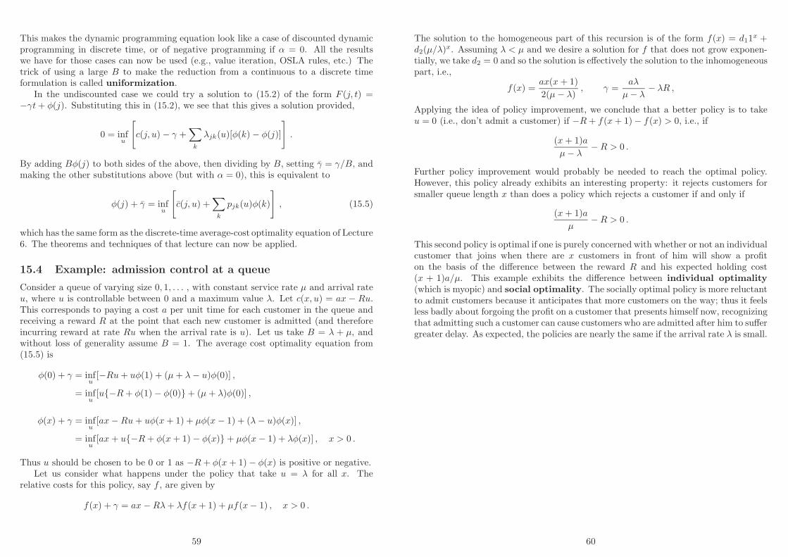
This makes the dynamic programming equation look like a case of discounted dynamicprogramming in discrete time, or of negative programming if α = 0. All the resultswe have for those cases can now be used (e.g., value iteration, OSLA rules, etc.) Thetrick of using a large B to make the reduction from a continuous to a discrete timeformulation is called uniformization.

In the undiscounted case we could try a solution to (15.2) of the form F (j, t) =−γt + φ(j). Substituting this in (15.2), we see that this gives a solution provided,

0 = infu

[

c(j, u) − γ +∑

k

λjk(u)[φ(k) − φ(j)]

]

.

By adding Bφ(j) to both sides of the above, then dividing by B, setting γ = γ/B, andmaking the other substitutions above (but with α = 0), this is equivalent to

φ(j) + γ = infu

[

c(j, u) +∑

k

pjk(u)φ(k)

]

, (15.5)

which has the same form as the discrete-time average-cost optimality equation of Lecture6. The theorems and techniques of that lecture can now be applied.

15.4 Example: admission control at a queue

Consider a queue of varying size 0, 1, . . . , with constant service rate µ and arrival rateu, where u is controllable between 0 and a maximum value λ. Let c(x, u) = ax − Ru.This corresponds to paying a cost a per unit time for each customer in the queue andreceiving a reward R at the point that each new customer is admitted (and thereforeincurring reward at rate Ru when the arrival rate is u). Let us take B = λ + µ, andwithout loss of generality assume B = 1. The average cost optimality equation from(15.5) is

φ(0) + γ = infu

[−Ru + uφ(1) + (µ + λ − u)φ(0)] ,

= infu

[u{−R + φ(1) − φ(0)} + (µ + λ)φ(0)] ,

φ(x) + γ = infu

[ax − Ru + uφ(x + 1) + µφ(x − 1) + (λ − u)φ(x)] ,

= infu

[ax + u{−R + φ(x + 1) − φ(x)} + µφ(x − 1) + λφ(x)] , x > 0 .

Thus u should be chosen to be 0 or 1 as −R + φ(x + 1) − φ(x) is positive or negative.Let us consider what happens under the policy that take u = λ for all x. The

relative costs for this policy, say f , are given by

f(x) + γ = ax − Rλ + λf(x + 1) + µf(x − 1) , x > 0 .

59

The solution to the homogeneous part of this recursion is of the form f(x) = d11x +

d2(µ/λ)x. Assuming λ < µ and we desire a solution for f that does not grow exponen-tially, we take d2 = 0 and so the solution is effectively the solution to the inhomogeneouspart, i.e.,

f(x) =ax(x + 1)

2(µ − λ), γ =

aλ

µ − λ− λR ,

Applying the idea of policy improvement, we conclude that a better policy is to takeu = 0 (i.e., don’t admit a customer) if −R + f(x + 1) − f(x) > 0, i.e., if

(x + 1)a

µ − λ− R > 0 .

Further policy improvement would probably be needed to reach the optimal policy.However, this policy already exhibits an interesting property: it rejects customers forsmaller queue length x than does a policy which rejects a customer if and only if

(x + 1)a

µ− R > 0 .

This second policy is optimal if one is purely concerned with whether or not an individualcustomer that joins when there are x customers in front of him will show a profiton the basis of the difference between the reward R and his expected holding cost(x + 1)a/µ. This example exhibits the difference between individual optimality(which is myopic) and social optimality. The socially optimal policy is more reluctantto admit customers because it anticipates that more customers on the way; thus it feelsless badly about forgoing the profit on a customer that presents himself now, recognizingthat admitting such a customer can cause customers who are admitted after him to suffergreater delay. As expected, the policies are nearly the same if the arrival rate λ is small.

60

16 Controlled Diffusion Processes

We give a brief introduction to controlled continuous-time stochastic models with acontinuous state space, i.e., controlled diffusion processes.

16.1 Diffusion processes and controlled diffusion processes

The Wiener process {B(t)}, is a scalar process for which B(0) = 0, the incrementsin B over disjoint time intervals are statistically independent and B(t) is normallydistributed with zero mean and variance t. (‘B’ stands for Brownian motion.) Thisspecification is internally consistent because, for example,

B(t) = B(t1) + [B(t) − B(t1)]

and for 0 ≤ t1 ≤ t the two terms on the right-hand side are independent normal variablesof zero mean and with variance t1 and t − t1 respectively.

If δB is the increment of B in a time interval of length δt then

E(δB) = 0 , E[(δB)2] = δt , E[(δB)j ] = o(δt) , for j > 2 ,

where the expectation is one conditional on the past of the process. Note that since

E[(δB/δt)2] = O[(δt)−1

]→ ∞ ,

the formal derivative ǫ = dB/dt (continuous-time ‘white noise’) does not exist in amean-square sense, but expectations such as

E

[{∫

α(t)ǫ(t)dt

}2]

= E

[{∫

α(t)dB(t)

}2]

=

∫

α(t)2dt

make sense if the integral is convergent.Now consider a stochastic differential equation

δx = a(x, u)δt + g(x, u)δB ,

which we shall write formally as

x = a(x, u) + g(x, u)ǫ .

This, as a Markov process, has an infinitesimal generator with action

Λ(u)φ(x) = limδt↓0

E

[φ(x(t + δt)) − φ(x)

δt

∣∣∣∣x(t) = x, u(t) = u

]

= φxa + 12φxxg2

= φxa + 12Nφxx ,

61

where N(x, u) = g(x, u)2. So this controlled diffusion process has DP equation

infu

[c + Ft + Fxa + 1

2NFxx

]= 0 , (16.1)

and in the vector case

infu

[c + Ft + Fxa + 1

2 tr(NFxx)]

= 0 .

16.2 Example: noisy LQ regulation in continuous time

The dynamic programming equation is

infu

[x⊤Rx + u⊤Qu + Ft + F⊤

x (Ax + Bu) + 12 tr(NFxx)

]= 0 .

In analogy with the discrete and deterministic continuous cases that we have consideredpreviously, we try a solution of the form,

F (x, t) = x⊤Π(t)x + γ(t) .

This leads to the same Riccati equation as in Section 12.2,

0 = x⊤

[

R + ΠA + A⊤Π − ΠBQ−1B⊤Π +dΠ

dt

]

x ,

and also, as in Section 7.3,

dγ

dt+ tr(NΠ(t)) = 0, giving γ(t) =

∫ T

t

tr(NΠ(τ)) dτ .

16.3 Example: a noisy second order system

Consider a special case of LQ regulation:

minimizeu

E

[

x(T )2 +

∫ T

0

u(t)2 dt

]

where for 0 ≤ t ≤ T ,

x(t) = y(t) and y(t) = u(t) + ǫ(t) ,

u(t) is the control variable, and ǫ(t) is Gaussian white noise,

Note that if we define z(t) = x(t) + (T − t)y(t) then

z = x − y + (T − t)y = (T − t)u + (T − t)ǫ(t)

where z(T ) = x(T ). Hence the problem can be posed only in terms of scalars u and z.

62

Recalling what we know about LQ models, let us conjecture that the optimalityequation is of a form

V (z, t) = z2Pt + γt . (16.2)

We could use (16.1). But let us argue from scratch. For (16.2) to work we will need

z2Pt + γt = minu

{u2δ + E

[(z + zδ)2Pt+δ + γt+δ

]}

= minu

{u2δ +

[z2 + 2(T − t)zuδ + (T − t)2δ

]Pt+δ + γt+δ

}+ o(δ)

The optimizing u isu = −(T − t)Pt+δz .

Substituting this and letting δ → 0 we have

−z2Pt − γt = −z2(T − t)2P 2t + (T − t)2Pt .

Thus−γt = (T − t)2Pt

andPt = (T − t)2P 2

t .

Using the boundary condition PT = 1, we find that the solution to the above differentialequation is

Pt =(1 + 1

3 (T − t)3)−1

,

and the optimal control is

u(t) = −(T − t)(1 + 1

3 (T − t)3)−1

z(t) .

16.4 Example: passage to a stopping set

Consider a problem of movement on the unit interval 0 ≤ x ≤ 1 in continuous time,x = u+ ǫ, where ǫ is white noise of power v. The process terminates at time T when xreaches one end or the other of the the interval. The cost is made up of an integral term12

∫ T

0(L + Qu2)dt, penalising both control and time spent, and a terminal cost which

takes the value C0 or C1 according as termination takes place at 0 or 1.Show that in the deterministic case v = 0 one should head straight for one of the

termination points at a constant rate and that the value function F (x) has a piecewiselinear form, with possibily a discontinuity at one of the boundary points if that boundarypoint is the optimal target from no interior point of the interval.

Show, in the stochastic case, that the dynamic programming equation with thecontrol value optimized out can be linearised by a transformation F (x) = α log φ(x) fora suitable constant α, and hence solve the problem.

Solution. In the deterministic case the optimality equation is

infu

[L + Qu2

2+ u

∂F

∂x

]

= 0, 0 < x < 1, (16.3)

63

with boundary conditions F (0) = C0, F (1) = C1. If one goes (from x) for x = 0 atspeed w one incurs a cost of C0 + (x/2w)(L + Qw2) with a minimum over w value ofC0 + x

√LQ. Indeed (16.3) is solved by

F (x) = min[

C0 + x√

LQ, C1 + (1 − x)√

LQ]

.

The minimizing option determines the target and the optimal w is√

L/Q.In the stochastic case

infu

[L + Qu2

2+ u

∂F

∂x+

v

2

∂2F

∂x2

]

= 0.

So u = −Q−1Fx and

L − Q−1

(∂F

∂x

)2

+ v∂2F

∂x2= 0 .

Make the transform F (x) = −Qv log φ(x) so φ(x) = e−F (x)/Qv. Then

Qv2 ∂2φ

∂x2− Lφ = 0 ,

with solutionφ(x) = k1 exp

(x

v

√

L/Q)

+ k2 exp(

−x

v

√

L/Q)

.

We choose the constants k1, k2 to meet the two boundary conditions on F .

0 0.2 0.4 0.6 0.81

1

1.2

1.4

1.6

1.8

2.0

2.2

v = 1

v = 2

v = 0.5

v = 0.25

v = 0.125

F (x) against x for the passage to a stopping set

The figure shows the solution for L = 1, Q = 4, C0 = 1, C1 = 1.5 and v = 0.125,0.25, 0.5, 1, 2 and the deterministic solution. Notice that noise actually reduces costby lessening the time until absorption at one or the other of the endpoints.

64

Index

adjoint variable, 49average-cost, 21

bang-bang control, 6Bellman equation, 3Brownian motion, 61

certainty equivalence, 43chattering, 47closed loop, 3control variable, 2controllability, 29controllable, 29controlled diffusion process, 61, 62

decomposable cost, 4diffusion process, 61discounted programming, 11discounted-cost criterion, 9discrete-time, 2dynamic programming equation, 3

feedback, 3finite actions, 15fixed terminal time, 53free terminal time, 53

gain matrix, 27Gaussian white noise, 62

Hamilton Jacobi Bellman equation, 45Hamiltonian, 49

individual optimality, 60infinitesimal generator, 57innovation process, 40innovations, 42interchange argument, 10

linear least squares estimate, 41LQG model, 25

Markov decision process, 4

Markov dynamics, 4Markov jump process, 58Markov policy, 17myopic policy, 16

negative programming, 11

observability, 37observable, 37one-step look-ahead rule, 18open loop, 3optimality equation, 3optimization over time, 1

perfect state observation, 4plant equation, 3policy, 3policy improvement, 23policy improvement algorithm, 24Pontryagin’s maximum principle, 49positive programming, 11power, 63principle of optimality, 2

r-controllable, 29r-observable, 37regulation, 25Riccati equation, 27

separation principle, 43social optimality, 60stability matrix, 33stabilizable, 33state variable, 3stationary Markov policy, 17stochastic differential equation, 61stopping problem, 18successive approximation, 14switching locus, 51

time horizon, 2time to go, 5

65

time-homogeneous, 5, 10transition intensity, 57transversality conditions, 50

uniformization, 59

value iteration, 14value iteration algorithm, 23value iteration bounds, 23

white noise, 27Wiener process, 61

66