OPTIMAL RESOURCE ALLOCATION IN WIRELESS COMMUNICATIONS

SUBJECT TO SEVERAL POWER AND ENERGY CONSTRAINTS

A Thesis

Submitted to the Graduate School

of the University of Notre Dame

in Partial Fulfillment of the Requirements

for the Degree of

Master of Science

in

Electrical Engineering

by

Mostafa Khoshnevisan,

J. Nicholas Laneman, Director

Graduate Program in Electrical Engineering

Notre Dame, Indiana

April 2011

c© Copyright by

Mostafa Khoshnevisan

2011

All Rights Reserved

OPTIMAL RESOURCE ALLOCATION IN WIRELESS COMMUNICATIONS

SUBJECT TO SEVERAL POWER AND ENERGY CONSTRAINTS

Abstract

by

Mostafa Khoshnevisan

It is known that adaptive power and rate allocation is a useful technique for

combating channel variations induced by multipath fading in wireless systems.

We consider several fading channel models for which we aim to optimize a perfor-

mance metric subject to various power and energy constraints. First, we find the

general structure of optimal or suboptimal power policies in order to maximize

the ergodic capacity subject to various combination of short-term, long-term, and

per-antenna power constraints in multiple-input multiple-output (MIMO) wire-

less systems. The power policies depend upon the ratio of the power constraints.

Furthermore, we characterize the conditions for which one or more power con-

straints dominates and the others can be ignored. Next, we specialize the results

to Rayleigh fading. An important observations in this case is that the short-term

power constraint is more relevant in the low SNR regime. Therefore, a system

designer can ignore a short-term power constraint that is larger than a long-term

power constraint for large values of average SNR’s. Finally, we consider an energy

harvesting wireless system, and study rate allocation policies to minimize a delay

criterion, e.g., average delay in the data buffer or probability of overflow, subject

to the hard power constraints imposed by the available energy.

To My Lovely Aunt Fereshteh

Whom I Lost This Year

and to Her Nice Husband, Mahmoud

and Her Adorable Children, Amin and Sara

ii

CONTENTS

FIGURES . . . . . . . . . . . . . . . . . . . . . . . . . . . . . . . . . . . . v

ACKNOWLEDGMENTS . . . . . . . . . . . . . . . . . . . . . . . . . . . vi

CHAPTER 1: INTRODUCTION . . . . . . . . . . . . . . . . . . . . . . . 11.1 Power Constraints and Their Practical Importance . . . . . . . . 11.2 Outline and Summary of Contributions . . . . . . . . . . . . . . . 6

CHAPTER 2: BACKGROUND . . . . . . . . . . . . . . . . . . . . . . . . 92.1 Throughput-Based Objective Functions . . . . . . . . . . . . . . . 92.2 Delay-Based Objective Functions . . . . . . . . . . . . . . . . . . 17

CHAPTER 3: LONG-TERM, SHORT-TERM, AND PER-ANTENNA POWERCONSTRAINTS . . . . . . . . . . . . . . . . . . . . . . . . . . . . . . 213.1 Channel Model and Problem Statement . . . . . . . . . . . . . . . 213.2 SISO Channels . . . . . . . . . . . . . . . . . . . . . . . . . . . . 233.3 MIMO Channels . . . . . . . . . . . . . . . . . . . . . . . . . . . 26

3.3.1 Long-Term and Short-Term Power Constraints . . . . . . . 273.3.2 Long-Term and Per-Antenna Power Constraints . . . . . . 333.3.3 Long-Term, Short-Term, and Per-Antenna Power Constraints 36

3.4 Summary . . . . . . . . . . . . . . . . . . . . . . . . . . . . . . . 40

CHAPTER 4: SPECIALIZING TO RAYLEIGH FADING . . . . . . . . . 424.1 Analysis . . . . . . . . . . . . . . . . . . . . . . . . . . . . . . . . 42

4.1.1 SISO and MISO . . . . . . . . . . . . . . . . . . . . . . . . 424.1.2 MIMO . . . . . . . . . . . . . . . . . . . . . . . . . . . . . 48

4.2 Numerical Results and Discussion . . . . . . . . . . . . . . . . . . 494.2.1 SISO and MISO . . . . . . . . . . . . . . . . . . . . . . . . 494.2.2 MIMO . . . . . . . . . . . . . . . . . . . . . . . . . . . . . 55

4.3 Summary . . . . . . . . . . . . . . . . . . . . . . . . . . . . . . . 60

iii

CHAPTER 5: HARD POWER CONSTRAINTS IN ENERGY HARVEST-ING SYSTEMS . . . . . . . . . . . . . . . . . . . . . . . . . . . . . . . 625.1 Model and Problem Statement . . . . . . . . . . . . . . . . . . . . 625.2 Main Results . . . . . . . . . . . . . . . . . . . . . . . . . . . . . 675.3 Multiple Access: Separate and Cooperative Users . . . . . . . . . 72

5.3.1 Separate Users . . . . . . . . . . . . . . . . . . . . . . . . 735.3.2 Cooperative Users . . . . . . . . . . . . . . . . . . . . . . 76

5.4 Summary . . . . . . . . . . . . . . . . . . . . . . . . . . . . . . . 77

CHAPTER 6: CONCLUSION . . . . . . . . . . . . . . . . . . . . . . . . . 796.1 Summary of Contributions . . . . . . . . . . . . . . . . . . . . . . 796.2 Future Work . . . . . . . . . . . . . . . . . . . . . . . . . . . . . . 81

BIBLIOGRAPHY . . . . . . . . . . . . . . . . . . . . . . . . . . . . . . . 85

iv

FIGURES

2.1 Illustration of water-filling in time . . . . . . . . . . . . . . . . . . 11

2.2 Illustration of modified water-filling in time . . . . . . . . . . . . . 15

2.3 The system model in [22] . . . . . . . . . . . . . . . . . . . . . . . 16

2.4 The system model in [4] . . . . . . . . . . . . . . . . . . . . . . . 18

2.5 The system model in [30] . . . . . . . . . . . . . . . . . . . . . . . 19

3.1 Illustration of the optimal power allocation for a 2× 2 MIMO system 31

4.1 The value of αmax, the threshold separating Cases 2 and 3, versusaverage SNR γ for SISO and MISO systems with Rayleigh fading 50

4.2 Ergodic capacity versus average SNR for MISO systems with Rayleighfading, Pmax = 20(13dB) and N0 = 1, and n = 2, 10. . . . . . . . . 52

4.3 Ergodic capacity versus average SNR for MISO systems with Rayleighfading, n = 2 and α =∞ and α = 1. . . . . . . . . . . . . . . . . 54

4.4 The value of αmax, the threshold separating Cases 2 and 3, versusAverage SNR per parallel channel ( P

mN0) for MIMO systems with

Rayleigh fading. . . . . . . . . . . . . . . . . . . . . . . . . . . . . 56

4.5 Ergodic capacity versus average SNR per parallel channel ( PmN0

) for2× 2 MIMO systems with Rayleigh fading. . . . . . . . . . . . . . 57

5.1 System Model . . . . . . . . . . . . . . . . . . . . . . . . . . . . . 63

5.2 An example of feasible power region . . . . . . . . . . . . . . . . . 74

v

ACKNOWLEDGMENTS

I am indebted to many people for making this thesis possible. Greatest grat-

itude goes to my advisor, Dr. J. Nicholas Laneman, who has been a tremendous

source of inspiration, guidance, and encouragement. I truly appreciate the price-

less freedom he provided in choosing my research’s topic. The productive sug-

gestions he offered in both the group and individual meetings were certainly the

main motivation for me to start and complete this work.

The friendly and nice environment of the university of Notre Dame, especially

the JNL group, made my graduate life enjoyable. I would like to thank Brian

Dunn, Michael Dickens, Glenn Bradford, Ebrahim MolavianJazi, Utsaw Kumar,

Zhanwei Sun, and Peyman Hesami. I have also benefited a lot from the theoretical

discussions that I had with the members of the group.

Finally, I would like to express my especial thanks to my family for their love

and support. My warm feelings and deep thanks are for my father, mother, sister,

and grandparents.

vi

CHAPTER 1

INTRODUCTION

In wireless systems, it is of great importance to adaptively allocate resources

such as power or rate in order to maximize a performance metric and at the same

time make sure to not violate the constraints imposed by rules and regulations

or system design limitations. The goal of this thesis is to precisely formulate a

variety of constraints and limitations in real-world systems and study the optimal

resource allocations for such systems. Optimizing a desired performance metric

subject to simultaneous power constraints with the assumption of channel state

information (CSI) at both the receiver and transmitter forms the core of this thesis.

In this chapter, we first discuss the importance of each of the power constraints

we consider in the thesis, and then summarize our contributions.

1.1 Power Constraints and Their Practical Importance

In real-world wireless communication systems, there are several important lim-

itations on the transmitter and its transmitted signal that might vary according

to the application. A combination of some or all of these constraints might be

necessary for a practical system.

One limitation results from the battery life of the mobile, which is captured by

long-term power constraints. A long-term power constraint can be mathematically

1

stated in the time-domain as

1

T1

∫ T1

0

NT∑k=1

x2k(t) dt ≤ P , (1.1)

where xk(t) is the output signal of the kth antenna at time t, and NT is the

number of antennas at the transmitter. The period of time T1 is assumed to be

large enough such that it contains many coherence times of the fading channel,

allowing the time-averaged long-term power constraint in (1.1) to be expressed in

terms of ensemble average over the Gaussian codewords and also over the fading

coefficients. This power constraint is meaningful if the mobile is equipped with

a battery that can be charged periodically with period T1, since in this case the

energy constraint imposed by the available energy in the battery of the mobile

can be expressed as the long-term power constraint in (1.1).

Another limitation results from regulations and rules that prevent the trans-

mitter from having an arbitrary power level due to environmental safety as well

as interference prevention. According to the Federal Communication Commis-

sion (FCC), the transmit power in any time duration should not exceed a certain

amount depending on the application, frequency, height of the antenna, popula-

tion of that area per square mile, and so on [1].

This regulatory constraint is captured by short-term power constraints, and it

can be mathematically stated in the time-domain as

1

T2

∫ T2

0

NT∑k=1

x2k(t) dt ≤ Pmax, (1.2)

where T2 � T1 is the shorter period of time over which the input power is

measured. With the block-fading channel model considered in this thesis, T2 is

2

assumed to be the block length, and T1 is assumed to be the channel coding length.

Thus, the time average (1.2) is taken over only a single block and the inequality

should hold for each block.

The short-term power constraint described above mathematically is consistent

with FCC rules. The Electronic Code of Federal Regulations (e-CFR) contains

the following rule [1, Title 47, Part15, D]: “the peak power output as measured

over an interval of time equal to the frame rate or transmission burst of the

device under all conditions of modulation. Usually this parameter is measured

as a conducted emission by direct connection of a calibrated test instrument to

the equipment under test”. We can infer from this rule that the power constraint

should be imposed at the transmitter instead of the receiver or any intermediate

node between the transmitter and receiver in the category of this regulation,

which is the scenario we consider. Also, from the general technical requirements

of those regulations “peak transmit power must be measured over any interval

of continuous transmission using instrumentation calibrated in terms of an rms-

equivalent voltage” [1, Title 47, Part 27].

Additionally, the power constraint is based on a measurement of the maxi-

mum conducted output power [1, Title 47, Part15, C], which is defined as the

total transmit power delivered to all antennas and antenna elements averaged

across all symbols in the signaling alphabet when the transmitter is operating at

its maximum power level. The FCC regulations also emphasize that “The average

must not include any time intervals during which the transmitter is off or is trans-

mitting at a reduced power level” [1, Title 47, Part15, C]. Other than the FCC,

Out Of Band (OOB) emission requirements set by the International Telecommu-

nication Union (ITU) [23] can impose a similar short-term power constraint on

3

the input power.

It is important to note that FCC regulations are very broad and have different

categories, such as licensed and unlicensed communication, or intentional and

unintentional radiation, and are usually expressed as a spectrum mask constraint.

The rules that we outlined above arise in different categories of FCC regulations.

What we consider as the short-term power constraint is a simplified constraint,

which puts a limitation on the maximum transmission power level.

Before turning our attention to another limitation, note that more precise

terminologies for these first two constraints would be long-term average and short-

term average power constraints. As it can be seen mathematically in Chapter 3,

for the long-term average power constraint, the average is taken over both the

codewords and channel fading coefficients, while for the short-term average power

constraint, the average is taken only over the codewords and the constraint applies

to each channel fading coefficient. We use terminology for the power constraints

from [7], in which the authors study the delay-limited capacity subject to long-

term power constraint, short-term power constraint, or both.

A third limitation results from the practical considerations for radio design,

which is captured by the per-antenna power constraint and prevents the ampli-

fier at each transmit antenna from distortions or nonlinearity by bounding the

dynamic range of the power at each antenna [21]. This constraint can be stated

mathematically in the time-domain as

1

T2

∫ T2

0

x2k(t) dt ≤ P , k = 1, 2, ..., NT , (1.3)

i.e., without the summation over antennas in (1.2). In principle, per-antenna

power constraints can be specified as either long- or short-term constraints. How-

4

ever, we only consider short-term per-antenna power constraints, since long-term

per-antenna constraints are not important in practical system design.

In many scenarios, all of the above power constraints should be taken into

account. In Chapters 3 and 4, we consider the ergodic capacity of the channel as

the objective function, and aim to maximize it subject to long-term, short-term,

and per-antenna power constraints assuming that CSI is available at both the

transmitter and receiver.

Finally, in some practical situations, instead of long-term power constraints,

we should consider energy constraints. This can happen if the device has not

the ability of getting fully recharged periodically. In energy harvesting wireless

systems, the users communicate with each other in a fading environment and

they harvest energy from a variety of sources and store it in an energy buffer such

as a capacitor or battery. In such systems, the input power is subject to hard

power constraints, i.e., the amount of energy consumed at each instant should not

exceed the amount of energy harvested in the energy buffer, which in the case of

single-input single-output (SISO) systems can be stated as

∫ (m+1)T2

mT2

x2(t) dt ≤ Eremm , m = 0, 1, ..., (1.4)

where T2 is the length of the block as before, and Eremm is the amount of energy

remained in the energy buffer at time mT2. In (1.4), we assume that energy arrives

into the energy buffer only at the start of each fading block. It is clear that in

energy harvesting systems, long-term power constraints are not relevant.

Energy harvesting has attracted considerable attention recently due to its

cheap, green, renewable, and naturally-presented source of energy. Solar, ther-

mal, kinetic, and wind are examples of such sources of energy. Energy harvesting

5

systems have a well-known application in powering low-energy electronics for wire-

less sensor networks. We consider a system model in which data and energy arrives

randomly due to a data and an energy arrival process and are stored in the data

and energy buffer, respectively. In the described system, the question then natu-

rally arises how we should spend the harvested energy to transmit the bits in the

data buffer for a given objective function. In addition to ergodic capacity, delay

is an important performance metric in wireless communications. Therefore, one

might optimize over all power policies in order to minimize delay subject to the

hard power constraints, which is the subject of Chapter 5.

1.2 Outline and Summary of Contributions

Chapter 2 reviews the literature and related works. In Chapter 3, we study

the general structure of optimal and suboptimal power allocation to maximize

the ergodic capacity subject to a combination of long-term, short-term, and per-

antenna power constraints with the assumption of CSI at both the transmitter

and the receiver. We consider SISO, multiple-input single-output (MISO), and

multiple-input multiple-output (MIMO) systems. We also characterize the situa-

tions for which one or more power constraints dominates and the others can be

ignored. The general structure of the power allocation policies depend upon the

ratio of the power constraints, number of antennas, and average signal-to-noise-

ratio (SNR) of the system.

In Chapter 4, we specialize the results of Chapter 3 to Rayleigh fading and

provide numerical results that illustrate the SNR regimes in which one or more

of the power constraints can be ignored. For each channel model we consider, we

quantify these regimes. Furthermore, these numerical results suggest that if the

6

input power is subject to long- and short-term power constraints, a short-term

power constraint that is larger than a long-term power constraint does not signifi-

cantly impact the ergodic capacity of the channel, for large average SNRs in MISO

systems and for all plotted average SNRs in MIMO systems. In other words, if

the short-term power constraint is larger than the long-term power constraint, the

difference between the capacity of a Rayleigh fading channel with optimal power

allocation subject to the long-term power constraint only and the capacity under

both long- and short-term power constraints is relatively small. This observation

suggests that some rules imposed by the FCC do not really constrain the sys-

tem design in the high SNR regimes for Rayleigh fading model, if the required

long-term power constraint stays less than the short-term power constraint.

In Chapter 5, we consider an energy harvesting wireless system in which the

data and energy arrive randomly due to different arrival processes, and the trans-

mitter adapts the transmission rate and power based on CSI and the state of data

and energy buffers such that the hard power constraints are satisfied. Two differ-

ent delay-based objective functions are considered in this part of the thesis. One

is the average delay incurred by the data, where the average is taken over all the

random processes in the system, i.e., data arrivals, energy arrivals, and the fading

process. When we consider this objective function, we assume that the buffer size

is infinite. Another objective function is the probability of overflow of the data

buffer, since the size of such buffers are limited in practice. If the size of the data

buffer is finite, then the probability that the buffer is full is a function of the buffer

size. Each of these objective functions can be expressed as an average cost for the

data buffers. With these assumptions, we prove that if the average rate of the

data arrivals is larger than a certain threshold, then the probability of overflow

7

is lower bounded by a constant, and the average delay is infinite when there is

no limitation on the buffer size. This threshold is basically the maximum average

rate of data subject to the energy constraints while the data buffer is removed.

On the other hand, if the average rate of the data arrivals is smaller than this

threshold and the buffer size is L, then we prove that there exists a sequence of

simple policies such that the probability of overflow goes to zero with a fast rate.

Finally, Chapter 6 concludes the thesis and discusses directions for future

research.

8

CHAPTER 2

BACKGROUND

There is a large body of literature on the subject of resource allocation in wire-

less systems that develops rate or power policies in order to optimize a performance

metric. Two important performance metrics in this literature are throughput-

based and delay-based metrics. In this chapter, we summarize important and

relevant works, and briefly describe their assumptions and state their results.

This chapter is not meant to be exhaustive. For a more complete overview, we

refer the readers to the references of this thesis.

2.1 Throughput-Based Objective Functions

In most resource allocation problems, a throughput-based objective function

such as ergodic capacity is maximized subject to some of the power constraints

described in Chapter 1. Ergodic capacity would be a relevant metric for scenarios

with fast fading. If the delay allowed by the application is much longer that

the coherence time of the channel, then the fading is called fast, which is the case

for non-delay-sensitive applications, such as data transmission as opposed to voice

communication. Assumptions on CSI at the receiver and transmitter vary in these

works, but in most of the cases, it is assumed that CSI is available at both the

receiver and transmitter.

9

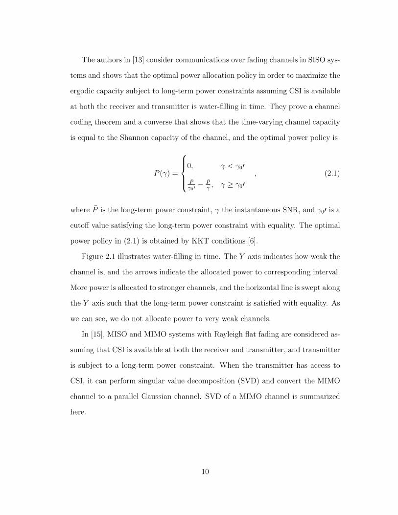
The authors in [13] consider communications over fading channels in SISO sys-

tems and shows that the optimal power allocation policy in order to maximize the

ergodic capacity subject to long-term power constraints assuming CSI is available

at both the receiver and transmitter is water-filling in time. They prove a channel

coding theorem and a converse that shows that the time-varying channel capacity

is equal to the Shannon capacity of the channel, and the optimal power policy is

P (γ) =

0, γ < γ0′

Pγ0′ −

Pγ, γ ≥ γ0′

, (2.1)

where P is the long-term power constraint, γ the instantaneous SNR, and γ0′ is a

cutoff value satisfying the long-term power constraint with equality. The optimal

power policy in (2.1) is obtained by KKT conditions [6].

Figure 2.1 illustrates water-filling in time. The Y axis indicates how weak the

channel is, and the arrows indicate the allocated power to corresponding interval.

More power is allocated to stronger channels, and the horizontal line is swept along

the Y axis such that the long-term power constraint is satisfied with equality. As

we can see, we do not allocate power to very weak channels.

In [15], MISO and MIMO systems with Rayleigh flat fading are considered as-

suming that CSI is available at both the receiver and transmitter, and transmitter

is subject to a long-term power constraint. When the transmitter has access to

CSI, it can perform singular value decomposition (SVD) and convert the MIMO

channel to a parallel Gaussian channel. SVD of a MIMO channel is summarized

here.

10

Figure 2.1. Illustration of water-filling in time

11

Consider the baseband-equivalent discrete-time model for a MIMO channel as

y = Hx + n,

where y is a complex vector of NR received signals, and x is a complex vector of NT

transmit signals. H and n are random sequences capturing the effect of multipath

fading and additive noise, respectively, and H at each time is an NR×NT matrix

of complex fading coefficients.

Let n := max (NR, NT ) and m := min (NR, NT ). The fading matrix H can be

represented using SVD as

H = UΛVH , (2.2)

where U and V are unitary matrices and Λ is a diagonal matrix with entries equal

to the square roots of the eigenvalues of the Wishart matrix

W =

HHH , if NR ≤ NT

HHH, if NR > NT

.

Denote the eigenvalues of W by λk, 1 ≤ k ≤ m. The equivalent channel model

is [25]

y = Λx + n, (2.3)

where we use the transformation y = UHy, x = VHx, and n = UHn. The

equivalent channel consists of m parallel channels. Note that the trace of the input

covariance matrix is invariant with respect to this transformation, e.g., tr(Qx) =

tr(Qx).

In the MISO case, the equivalent channel is a SISO system, and optimal power

policy is given by (2.1). In the MIMO case, however, the optimal power policy to

12

maximize the ergodic capacity is shown to be space-time water-filling (also known

as matrix water-filling), which takes the form

Pk =

(1

v′− P

mλ′k

)+

,

where λ′k is the kth normalized singular value of the channel matrix and the con-

stant v′ is determined by substituting the above power policy into

Eλ′[

m∑k=1

Pk(λ′)

]= P ,

which is basically chosen such that the long-term power constraint is satisfied with

equality.

Multiuser scenarios under long-term power constraints are considered in [17]

and [28]. In [17], the optimal power policy to maximize the ergodic sum-of-rates

capacity of a multiple access channel is derived, and it turns out that only one

user can transmit at any particular time instant, and each user allocates power in

time based on the water-filling policy in (2.1). In [28], the whole capacity region

and the corresponding power policies are obtained by extracting the polymatriod

structure of the capacity region.

In some other works, a short-term power constraint is considered. Telatar

in [25] studies the capacity of a MIMO channel subject to a short-term power

constraint for complete CSI, and for CSI at the receiver only. Using singular

value decomposition (SVD), he shows that the optimal power policy is water-

filling across space. Another example of evaluating the capacity subject to only a

short-term power constraint is [12], in which the authors provide an overview of the

results on the Shannon capacity of MIMO channels under different assumptions

on availability of CSI or channel distribution information (CDI).

13

Another power constraint that arises in this thesis is a per-antenna power con-

straint. In [14], per-antenna power constraints are considered in MIMO wireless

systems in the context of beamforming with incomplete CSI. Also, [9] studies op-

timal power allocation subject to `p-norm constrained eigenvalues, which can be

viewed as a suboptimal power allocation policy under short-term and per-antenna

power constraints.

Maximizing the ergodic capacity subject to multiple simultaneous power con-

straints is also considered in some works. The authors in [16] prove a similar

coding theorem to the one in [13] for the Shannon capacity of a SISO fading chan-

nel subject to both long- and short-term power constraints, and state that the

optimal power policy is

P (γ) =

0, γ < γ0

Pγ0− P

γ, γ0 ≤ γ < γ1

Pmax, γ1 ≤ γ

, (2.4)

where P and Pmax are the long- and short-term power constraints, respectively, γ

is the instantaneous SNR, and the thresholds γ0 and γ1 are determined from the

following equations

P

γ0

− P

γ= Pmax, (2.5)

Eγ [P (γ)] = P .

The power policy in (2.4) is obtained by KKT conditions [6]. We call this

power policy modified water-filling across time, where we do not let the power

level exceed the short-term power constraint and the thresholds are obtained such

14

that the long-term power constraint is satisfied with equality.

Figure 2.2 illustrates the modified water-filling in time. The Y axis indicates

how weak the channel is, and the arrows indicate the allocated power to the

corresponding interval. More power is allocated to stronger channels, but we do

not let the power level exceed Pmax, and the horizontal line is swept along the Y

axis such that the long-term power constraint is satisfied with equality. We do

not allocate power to very weak channels under a certain threshold.

Figure 2.2. Illustration of modified water-filling in time

15

As we discuss further in Chapter 3, this policy (2.4) is optimal only in one

regime. The authors in [8] study the same problem for multiple access channels.

We study the optimal power allocation in fast fading MIMO systems subject

to long-term, short-term, and per-antenna power constraints, as continue of the

current literature described above.

Capacity of fast fading Gaussian channel with an energy harvesting sensor

node is studied in [22], with the system model they consider shown in Figure 2.3.

Figure 2.3. The system model in [22]

The ergodic capacity of a fast fading channel subject to energy constraints is

studied. The authors of [22] argue that the ergodic capacity for this model is the

same as the ergodic capacity of a fast fading channel subject to a certain long-term

power constraint, and the optimal power control is water-filling in time.

16

2.2 Delay-Based Objective Functions

Another important performance metric in wireless communications is delay.

It is known that to achieve the ergodic capacity of a fast fading channel one

needs to code across many coherence time of the channel, which requires a large

delay. In fact, fast fading is a relevant metric when the delay requirement of the

application is much larger than the coherence times of the channel. In delay-

sensitive applications, we might focus on a minimal delay communication rather

than on maximal rate communication. With this consideration, we might be

allowed to code across only a single block or across finitely many coherence times

of the channel.

Delay-based objective functions usually arise in network theory if data sources

are considered to be bursty. These aspects have not been fully taken into account

by information theory. The authors in [19] introduce a framework in which some

aspects of both networking and information theory are incorporated. In this work,

delay-optimal scheduling policies for channels with constant latency are obtained

and shown to be threshold strategies, and some properties of optimal policies for

channels with affine latency are derived.

The authors in [4] consider a fading channel between two users and assume

that the data arrives randomly due to a data arrival distribution and stores in a

data buffer until it is transmitted. They study adapting the user’s transmission

rate and power based on CSI and the data buffer occupancy. The system model

in [4] is shown in Figure 2.4.

Two scenarios are considered in [4]. The first scenario, which is based on the

mutual information model, corresponds to fixed-length/variable-rate codewords,

where each codeword is sent in one block of N channel uses, and thus the length

17

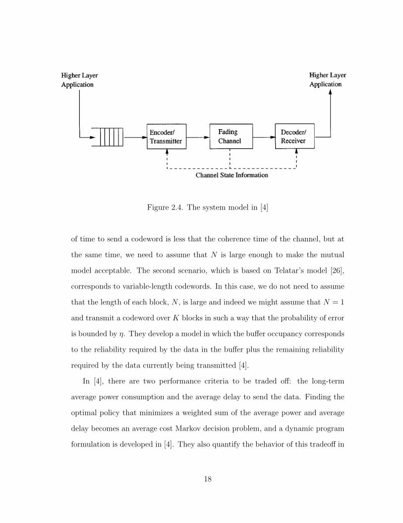
Figure 2.4. The system model in [4]

of time to send a codeword is less that the coherence time of the channel, but at

the same time, we need to assume that N is large enough to make the mutual

model acceptable. The second scenario, which is based on Telatar’s model [26],

corresponds to variable-length codewords. In this case, we do not need to assume

that the length of each block, N , is large and indeed we might assume that N = 1

and transmit a codeword over K blocks in such a way that the probability of error

is bounded by η. They develop a model in which the buffer occupancy corresponds

to the reliability required by the data in the buffer plus the remaining reliability

required by the data currently being transmitted [4].

In [4], there are two performance criteria to be traded off: the long-term

average power consumption and the average delay to send the data. Finding the

optimal policy that minimizes a weighted sum of the average power and average

delay becomes an average cost Markov decision problem, and a dynamic program

formulation is developed in [4]. They also quantify the behavior of this tradeoff in

18

the asymptotically large delay regime. Our work in Chapter 5 is based on the first

model (fixed-length variable-rate codewords) introduced in [4], but the energy is

harvested in our model and the objective is to minimize a delay criterion.

The authors in [30] consider an energy harvesting communication system over

a constant link. They assume an ideal situation in which the exact amount of data

and all energy arrivals are known to the transmitter a priori, and they develop an

off-line algorithm to minimize the transmission time of all the data up to a certain

time. The system model in this work is shown in Figure 2.5.

Figure 2.5. The system model in [30]

This model allows for relatively simple and explicit analysis by ignoring the

randomness of data and energy arrivals, and cannot be extended directly to fading

channels.

In Chapter 5, we consider a fading channel in which data and energy arrive

19

randomly, and are stored in data and energy buffers, respectively. We assume

that the the transmitter and receiver have access to causal information about the

channel state, data buffer occupancy, and energy buffer occupancy. Finding the

optimal rate policy to minimize the probability of overflow or average delay of the

data buffer is the aim of this part of our work.

20

CHAPTER 3

LONG-TERM, SHORT-TERM, AND PER-ANTENNA POWER

CONSTRAINTS

In this chapter, we first introduce the channel model and the general formula-

tion of our problem. Then, we study the problem for SISO and MIMO channels.

It is conceptually and notationally appealing to treat SISO and MIMO channels

separately, since in the SISO case the short-term power constraint coincides with

the per-antenna power constraint, because there is only one antenna at the trans-

mitter. On the other hand, the optimization problem is more intricate in the

MIMO case.

3.1 Channel Model and Problem Statement

The baseband-equivalent discrete-time input-output relationship in our MIMO

channel model is

y(i) = H(i)x(i) + n(i), (3.1)

where i is the time index, y(i) is a complex vector of NR received signals, x(i)

is a complex vector of NT transmit signals. H(i) and n(i) are random sequences

capturing the effect of multipath fading and additive noise, respectively. The noise

n(i) is a vector of NR zero-mean, circularly symmetric, complex Gaussian random

21

variables with E[n(i)n(i)H ] = N0INR , and n(i), i = 1, 2, ... is a sequence of inde-

pendent random vectors. The multipath fading H(i) at each time is an NR ×NT

matrix of complex fading coefficients. We assume that the matrix fading process

is stationary and ergodic, and that it varies slowly enough that CSI is available

to the receiver and transmitter. For the case of Rayleigh fading in Chapter 4,

we assume that the entries of H(i) are independent and identically distributed

(i.i.d.) complex Gaussian random variables with mean zero and variance 1/2 per

real dimension.

By considering this channel model and transferring the power constraints in

terms of time averages in Chapter 1 to the ensemble averages, the general optimiza-

tion problem for maximizing the ergodic capacity subject to long-term, short-term,

and per-antenna power constraints is

maxQ(H)

EH

[log det

(1 +

1

N0

HQ(H)HH

)], (3.2a)

subject to EH [tr(Q(H))] ≤ P , (3.2b)

∀H : tr(Q(H)) ≤ Pmax, (3.2c)

∀H : qkk(H) ≤ P , k = 1, 2, ..., NT , (3.2d)

where Q is the input covariance matrix, which needs to be maximized as a function

of the instantaneous channel and qkk is the kth diagonal entry of the matrix Q.

The expectations in (3.2a) and (3.2b) are with respect to the distribution of H.

The power constraints are described in (3.2b), (3.2c), and (3.2d); P represents

the long-term power constraint, Pmax represents the short-term power constraint,

and P represents the per-antenna power constraint. For simplicity, we drop the

time index i. This channel model and the optimization problem simplify to a

22

scalar/vector problem for the SISO/MISO cases considered in the sequel.

3.2 SISO Channels

We first obtain the optimal power allocation in a SISO system subject to both

long- and short-term power constraints. The channel model is the scalar form

of (3.1) with NT = NR = 1.

Let γ := P |h|2N0

denote the instantaneous received SNR without power adapta-

tion, where h is the scalar fading coefficient, and let f(γ) denote the probability

density function (pdf) of γ. Let P (γ) denote the power policy capturing the sec-

ond moment of the input signal as a function of γ. Then the received SNR with

power adaptation is P (γ)γ/P , and the ergodic capacity is [13]

C = Eγ[log

(1 +

P (γ)γ

P

)]. (3.3)

Based upon the coding theorem in [16], the ergodic capacity is the solution to the

following optimization problem:

maxP (γ)

∫log

(1 +

P (γ)γ

P

)f(γ) dγ, (3.4)

subject to Eγ [P (γ)] ≤ P ,

∀γ : P (γ) ≤ Pmax,

which corresponds to a scalar version of (3.2). To determine the general power

policy, let α := Pmax/P be the ratio of the short-term power constraint to the

long-term power constraint, and let αmax be a constant to be specified shortly,

and consider the following three cases:

23

Case 1, α ≤ 1: In this case, the short-term power constraint is always satisfied

with equality and the long-term power constraint can be ignored. Therefore, the

optimal power policy in this case is

P (γ) = Pmax,∀γ. (3.5)

Case 2, αmax ≤ α: In this case, it turns out we can ignore the short-term

power constraint, and the power policy is water-filling in time [13]

P (γ) =

0, γ < γ′0

Pγ′0− P

γ, γ ≥ γ′0

, (3.6)

where the threshold γ′0 is determined from substituting above power allocation

into

Eγ [P (γ)] = P . (3.7)

Case 3, 1 < α ≤ αmax: In this case both long- and short-term power con-

straints play a role, and the power allocation in [16] provides the solution to the

optimization problem as discussed in Chapter 2. By substituting γ1 from (2.5)

and put it into (2.4), the power allocation in this case becomes

P (γ) =

0, γ < γ0

Pγ0− P

γ, γ0 ≤ γ < γ0

1−αγ0

Pmax,γ0

1−αγ0≤ γ

, (3.8)

where the threshold γ0 is determined by substituting the above power allocation

into (3.7). This solution comes from the KKT conditions [6]. We call this power

24

policy modified water-filling across time, where we do not let the power level

to exceed the short-term power constraint and the threshold is obtained such

that the long-term power constraint is satisfied with equality. As we mentioned

previously, [16] determines a similar solution, which is valid only in this case

(Case 3), since the threshold γ0 in (3.8) has a valid solution only in this regime.

In Chapter 4, for the Rayleigh fading channel, we show that the threshold γ0 is

uniquely determined from (3.7) if 1 < α ≤ αmax (Case 3).

Note that the thresholds γ0 in (3.8) and γ′0 in (3.6) are, in general, different.

In order to eliminate the short-term power constraint, the power policy in (3.6)

should always satisfy the short-term power constraint P (γ) ≤ Pmax, ∀γ, but the

maximum value of P (γ) in (3.6) occurs as γ →∞ and is equal to P /γ′0. Therefore,

P

γ′0≤ Pmax ⇒ 1

γ′0≤ α ⇒ αmax =

1

γ′0. (3.9)

In general, the values of γ′0 and αmax depend on the distribution of γ and the

average SNR of the system. In Chapter 4, we find these values for a Rayleigh

fading channel analytically and numerically. It is worth mentioning that the value

of αmax is important in practical wireless communication systems, since it might

be the case that the allowed α is larger than αmax. In that case, we can simply

ignore the short-term power constraint, and the optimal power allocation policy

is water-filling in time.

We have discussed the power policies in Cases 2 and 3 in Chapter 2, which are

water-filling in time and modified water-filling in time, and the are illustrated in

Figures 2.1 and 2.2, respectively.

From e-CFR [1, Title 47, Part 27], we find the following rule: “In measuring

transmission in the 1710-1755 MHz and 2110-2155 MHz bands using an average

25

power technique, the peak-to-average ratio (PAR) of the transmission may not

exceed 13 dB.”In fact, as we will see from the numerical results in Section 4.2,

the value of αmax is less than 13 dB for all the channel models we consider at

an average SNR higher than -10 dB. Therefore, a system designer can simply

ignore the short-term power constraint in those regimes and use water-filing in

time as the power policy without violating the above rule. In other words, this

FCC constraint is quite liberal.

If there are multiple antennas at the transmitter and a single antenna at the

receiver, i.e., MISO, the problem of maximizing the ergodic capacity subject to

both long- and short-term power constraints is the same as the one in the SISO

case, since we can convert the MISO channel to an equivalent SISO channel. We

consider two different conversions for MISO systems: singular value decomposi-

tion (SVD),which is optimal, and antenna selection at the transmitter, which is

suboptimal. In Chapter 4, we derive the optimal power allocation policy for each

case and obtain the thresholds for the optimization problems in Rayleigh fading.

3.3 MIMO Channels

In this section we assume that there are multiple antennas at the transmitter

and the receiver. The channel model and problem statement are described in

Section 3.1. Consider the SVD method described in Chapter 2.

Let Λ′ :=√

PmN0

Λ be the normalized channel with diagonal entries equal to

square root of λ′k = PmN0

λk, 1 ≤ k ≤ m. In the SVD equivalent channel model, the

power allocation policy is a function of Λ′. Therefore, the covariance matrix can

be given as Q(Λ′) or Q(λ′), where λ′ := [λ′1, λ′2, ..., λ

′m]. To maximize the capacity,

the covariance matrix should be diagonal [25]. Let Pk(λ′), 1 ≤ k ≤ m denote the

26

kth diagonal entry of the covariance matrix. Note that each Pk is a function of

the vector λ′, or in other words, a function of all λ′l’s, 1 ≤ k, l ≤ m.

In the following three subsections, we obtain the power allocation that max-

imizes the ergodic capacity subject to various combinations of the three power

constraints described earlier. Optimal power allocations are obtained in Sec-

tion 3.3.1, but suboptimal solutions are obtained in Sections 3.3.2 and 3.3.3 due to

more stringent constraints. While not necessary in principle, these more stringent

constraints are more amendable to analysis.

3.3.1 Long-Term and Short-Term Power Constraints

If the input power is subject to long- and short-term power constraints, we

remove the constraint in (3.2d). Then, using the SVD equivalent channel model

and the above definitions, the optimization problem in (3.2) becomes

maxPk(λ′),k=1,2,...,m

C = Eλ′[

m∑k=1

log

(1 +

Pk(λ′)λ′k

P /m

)], (3.10)

subject to Eλ′[

m∑k=1

Pk(λ′)

]≤ P ,

∀λ′ :m∑k=1

Pk(λ′) ≤ Pmax.

The optimal power allocation structure can be found by examining the KKT

conditions. Formally, we state and prove the following theorem.

27

Theorem 1. The solution to the optimization problem (3.10) for P ≤ Pmax is

Pk(λ′) =

(

1v− P

mλ′k

)+

, if∑m

k=1

(1v− P

mλ′k

)+

≤Pmax(1

β+v− P

mλ′k

)+

, otherwise

, (3.11)

where (x)+ := max (0, x). The Lagrange multipliers v and β are obtaining by

solvingm∑k=1

(1

β + v− P

mλ′k

)+

= Pmax, (3.12)

Eλ′[

m∑k=1

Pk(λ′)

]= P . (3.13)

Proof. Since (3.10) is a convex optimization problem, We prove the theorem using

the KKT conditions [6]. For simplicity, we drop λ′ from Pk(λ′) and simply denote

it by Pk in the proof of Theorems 1, 2 and 3. To maximize the capacity, the

long-term power constraint should be satisfied with equality, which is possible

since α ≥ 1. Let θ1, θ2, ..., θm denote the Lagrange multipliers corresponding to

the constraints that force the powers to be positive (P1 ≥ 0, P2 ≥ 0, ..., Pm ≥ 0,

respectively), θ′ be the Lagrange multiplier corresponding to the short-term power

constraint, and v be the Lagrange multiplier corresponding to the long-term power

constraint (we consider the long-term power constraint with equality). Then, the

KKT conditions can be written as

28

θkPk = 0, k = 1, 2, ...,m, (3.14a)

θk ≥ 0, k = 1, 2, ...,m, (3.14b)

Pk ≥ 0, k = 1, 2, ...,m, (3.14c)

θ′(m∑k=1

Pk − Pmax) = 0, (3.14d)

θ′ ≥ 0, (3.14e)

m∑k=1

Pk ≤ Pmax, (3.14f)

− mf(λ′)

mPk + Pλ′k

− θk + θ′ + vf(λ′) = 0, k = 1, 2, ...,m, (3.14g)

Eλ′[

m∑k=1

Pk

]= P . (3.14h)

Now, based on the above conditions, we obtain some restrictions on the solu-

tion:

Restriction 1: if Pk 6= 0, then from (3.14a), θk = 0, so θ′ = ( 1Pk+P /(mλ′k)

−

v)f(λ′) ≥ 0 (from (3.14g) and (3.14e)).

Restriction 2: if Pmλ′k≥ 1

v, then Pk = 0 (from Restriction 1).

Now, consider two different situations:

Situation 1,∑m

k=1

(1v− P

mλ′k

)+

≤ Pmax: In this case, the power allocation

Pk =(

1v− P

mλ′k

)+

, 1 ≤ k ≤ m is a valid solution and satisfies all the KKT

conditions (note that in this case θ′ = 0, and from Restriction 1 and 2, above

power allocation results).

Situation 2,∑m

k=1

(1v− P

mλ′k

)+

> Pmax: In this case, θ′ 6= 0 and from (3.14d),

we have∑m

k=1 Pk − Pmax = 0. Now, consider two cases:

29

2.1: If Pmλ′k≥ 1

θ′/f(λ′)+v, then Pk = 0 (because if Pk > 0, then from (3.14a)

θk = 0, and from (3.14g) Pk = 1θ′/f(λ′)+v

− Pmλ′k

> 0, which is a contradiction).

2.2: If Pmλ′k

< 1θ′/f(λ′)+v

, then θk = 0 (because if θk > 0, then from (3.14a)

Pk = 0, and from (3.14g) θk = θ′+vf(λ′)− f(λ′)P /(mλ′k)

> 0, so Pmλ′k

> 1θ′/f(λ′)+v

, which

is a contradiction).

With the explanation in 2.1 and 2.2 cases, and defining β := θ′/f(λ′), we now

can determine the power allocation in situation 2. That is Pk =(

1β+v− P

mλ′k

)+

, 1 ≤

k ≤ m, where β is the answer to the equation∑m

k=1

(1

β+v− P

mλ′k

)+

= Pmax.

The power allocation described in Situation 1 and Situation 2 completes the

proof.

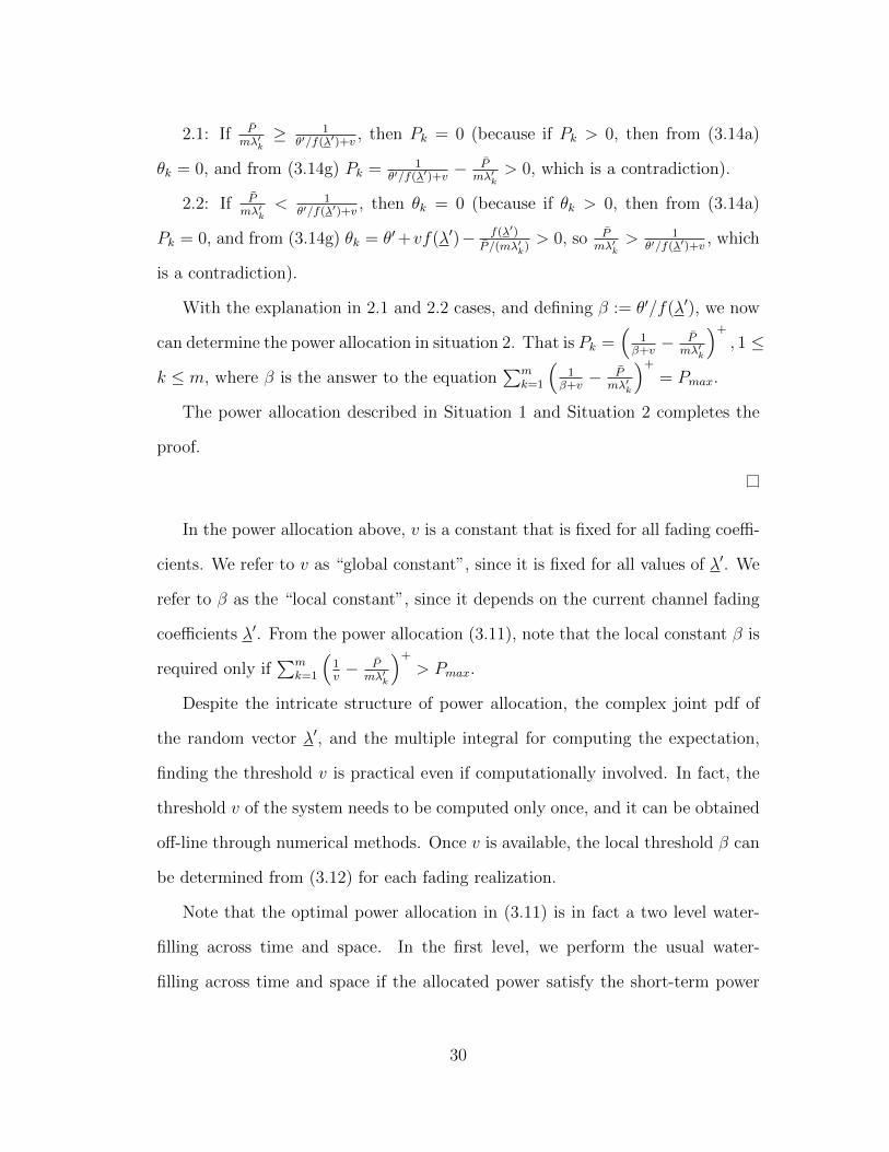
In the power allocation above, v is a constant that is fixed for all fading coeffi-

cients. We refer to v as “global constant”, since it is fixed for all values of λ′. We

refer to β as the “local constant”, since it depends on the current channel fading

coefficients λ′. From the power allocation (3.11), note that the local constant β is

required only if∑m

k=1

(1v− P

mλ′k

)+

> Pmax.

Despite the intricate structure of power allocation, the complex joint pdf of

the random vector λ′, and the multiple integral for computing the expectation,

finding the threshold v is practical even if computationally involved. In fact, the

threshold v of the system needs to be computed only once, and it can be obtained

off-line through numerical methods. Once v is available, the local threshold β can

be determined from (3.12) for each fading realization.

Note that the optimal power allocation in (3.11) is in fact a two level water-

filling across time and space. In the first level, we perform the usual water-

filling across time and space if the allocated power satisfy the short-term power

30

constraint. Otherwise, we penalize the power by adding the local constant β in

the denominator in (3.11) such that the short-term power constraint is satisfied

with equality. The illustration of the optimal power policy for a 2 × 2 MIMO

system in Figure 3.1 gives some useful insight about the structure of the power

allocation.

Figure 3.1. Illustration of the optimal power allocation for a 2× 2MIMO system

31

In Figure 3.1, the X axis indicates the time. For every time slot the value

of Pmλ′k

for k = 1, 2 for the two singular values of the channel is sketched. In

fact, the Y axis indicates how weak is the channel, and the arrows indicate the

allocated power to the corresponding channels. More power is allocated to stronger

channels, but we do not allow the sum of the allocated power corresponding to the

two singular values of the channel exceed the short-term power constraint Pmax at

each time slot. As it can be seen, at time slots 1, 2, 4, 5, and 7, the power policy

is water-filling across time and space. However, for time slots 3 and 6, we change

the threshold such that the sum of the power corresponding to the two singular

values of the channel is equal to the short-term power constraint. Note that the

constant β depends on the channel fading coefficients, and the global threshold v

is chosen such that the long-term power constraint is satisfied with equality.

In Section 3.2, finding the optimal power allocation was separated into three

cases depending on the value of α and a constant αmax. An analogous situation

arises for MIMO systems, as we now briefly discuss.

Case 1, α ≤ 1: In this case, the short-term power constraint is satisfied with

equality, and the long-term power constraint can be removed. The optimal power

allocation is the well-known water-filling across antennas, but not across time, as

obtained in [25].

Case 2, αmax ≤ α: In this case, the power allocation in Theorem 1 is valid,

but it simplifies to water-filling in time and space

Pk =

(1

v′− P

mλ′k

)+

, (3.15)

where the constant v′ is determined by substituting the above power policy into (3.13).

In fact, we can eliminate the short-term power constraint, and the problem re-

32

duces to finding the optimal power allocation for MIMO channels subject to only

a long-term power constraint, which has been examined in [15].

Case 3, 1 < α ≤ αmax: Both power constraints paly a role, and the optimal

power allocation is given by Theorem 1, which was discussed earlier.

The only remaining task is to obtain the value of αmax. Note that for this case,

we must ensure that the power allocation in (3.15) does not violate the short-term

power constraint. Therefore, we have

m∑k=1

(1

v′− P

mλ′k

)+

≤ Pmax,∀λ′ ⇒m∑k=1

1

v′≤ Pmax

⇒ m

v′P≤ Pmax

P.

Therefore, we have

αmax =m

v′P. (3.16)

3.3.2 Long-Term and Per-Antenna Power Constraints

If the input power is subject to long-term and per-antenna power constraints,

we remove the constraint in (3.2c). First, note that for a Hermitian matrix Q we

have [18]

max1≤k≤NT

qkk ≤ max1≤k≤NT

eigenvaluek(Q), (3.17)

where qkk is the kth diagonal entry of the matrix Q, and eigenvaluek(Q) is the

kth eigenvalue of the matrix Q. If we consider the SVD method discussed earlier,

then under the transformation x = VHx, the eigenvalues of the input covariance

matrix do not change. On the other hand, the eigenvalues of the matrix Qx are

33

equal to the diagonal entries Pk(λ′), 1 ≤ k ≤ m. Therefore, the constraint

Pk(λ′) ≤ P , k = 1, ...,m, (3.18)

is sufficient to satisfy (3.2d). Because of inequality (3.17), this condition is only

sufficient and not necessary. Therefore, we can find a suboptimal solution by

assuming a more stringent constraint. Specifically, we consider the optimization

problem

maxPk(λ′),k=1,2,...,m

C = Eλ′[

m∑k=1

log

(1 +

Pk(λ′)λ′k

P /m

)], (3.19)

subject to Eλ′[

m∑k=1

Pk(λ′)

]≤ P ,

∀λ′ : Pk(λ′) ≤ P , k = 1, ...,m.

Theorem 2. The solution to the optimization problem (3.19) for P ≤ mP is

Pk(λ′) =

0, if P

mλ′k≥ 1

v

1v− P

mλ′k, if 1

v> P

mλ′k≥ 1

v− P

P , otherwise

. (3.20)

Proof. Let θ1, θ2, ..., θm denote the Lagrange multipliers corresponding to the con-

straints that force the powers to be positive (P1 ≥ 0, P2 ≥ 0, ..., Pm ≥ 0, respec-

tively), θ′1, θ′2, ..., θ

′m be the Lagrange multipliers corresponding to the per-antenna

power constraints (P1 ≤ P , P2 ≤ P , ..., Pm ≤ P , respectively), and v be the La-

grange multiplier corresponding to the long-term power constraint (we consider

34

the long-term power constraint with equality). Then, the KKT conditions can be

written as [6]:

θkPk = 0, k = 1, 2, ...,m,

θk ≥ 0, k = 1, 2, ...,m,

Pk ≥ 0, k = 1, 2, ...,m,

θ′k(Pk − P ) = 0,

θ′k ≥ 0,

Pk ≤ P ,

− f(λ′)

Pk + Pmλ′k

− θk + θ′k + vf(λ′) = 0, k = 1, 2, ...,m,

Eλ′[

m∑k=1

Pk

]= P .

Then, with the same procedure as in the proof of Theorem 1, we can see that

the power policy in (3.20) results from above conditions.

Note that in the power allocation above, v is a constant that is fixed for all

fading coefficients, and is determined by substituting the power allocation (3.20)

into (3.13). Let α := mP/P . Note that the definition of α is slightly different

from Sections 3.2 and 3.3.1, since there are m per-antenna power constraints here.

Again, the general power allocation can be determined by considering three cases.

Case 1, α ≤ 1: In this case, the long-term power constraint can be removed

and the power policy is given by Pk(λ′) = P .

Case 2, αmax ≤ α: In this case, the per-antenna power constraint can be

removed. The power allocation in Theorem 2 is valid and simplifies to (3.15),

35

where v′ is determined from (3.13). By the same procedure as before, we can find

that αmax = m/(v′P ).

Case 3, 1 < α ≤ αmax: In this case, both power constraints play a role and

the power policy is given by (3.20).

3.3.3 Long-Term, Short-Term, and Per-Antenna Power Constraints

If the input power is subject to long-term, short-term, and per-antenna power

constraints, we obtain a suboptimal power allocation. The corresponding opti-

mization problem is given in (3.2). In order to make this optimization prob-

lem mathematically tractable, we will combine the two power constraints (3.2c)

and (3.2d) into a more stringer power constraint. Using [9, Lemma 1] and in-

equality (3.17), the following lemma applies.

Lemma 1. If Pmaxm≤ P ≤ Pmax, and the following p-norm power constraint is

satisfied

∀λ′ :

(m∑k=1

(Pk(λ′))

p

) 1p

≤ P , (3.21)

where p = ln (m)/ ln (mP/Pmax), then the two power constraints (3.2c) and (3.2d)

would be satisfied.

Proof. The proof follows from inequality (3.17), the described SVD method and

its properties, and [9, Lemma 1].

Note that the p-norm power constraint (3.21) is sufficient, not necessary.

Therefore, the power allocation in the sequel is suboptimal. Considering Lemma

1, the optimization problem in (3.2) can be stated as following.

36

maxPk(λ′),k=1,2,...,m

C = Eλ′[

m∑k=1

log

(1 +

Pk(λ′)λ′k

P /m

)], (3.22)

subject to Eλ′[

m∑k=1

Pk(λ′)

]≤ P ,

∀λ′ :

(m∑k=1

(Pk(λ′))

p

) 1p

≤ P .

Theorem 3. The solution to the optimization problem (3.22) for P ≤ mp−1p P , is

the optimal power allocation policy as

Pk(λ′) =

0, if Pmλ′k≥ 1

v

1v− P

mλ′k, if 1

v< P

mλ′kand

(∑mk=1

((1v′− P

mλ′k

)+)p) 1

p

≤ P

sol, otherwise

(3.23)

where sol in above equation is the solution of −v+(Pk(λ′)+ P

mλ′k)−1 = (Pk(λ

′))p−1

β,

and β is a constant depending on the fading coefficients and is chosen such that

the inequality (3.21) is satisfied with equality for the corresponding fading coeffi-

cient. The constant v like before, is a global constant, which is chosen such that

the long-term power constraint is satisfied with equality, i.e., is determined from

substituting the power allocation (3.23) into (3.13).

Proof. The proof is based on the KKT conditions, and is very similar to the proof

of Theorem 1. In fact, the KKT conditions are the same as in proof of Theorem 1,

but instead of the condition in (3.14d), (3.14f), and (3.14g), we have the following

37

conditions

θ′

((m∑k=1

P pk )

1p − P )

)= 0,

(m∑k=1

P pk )

1p ≤ P ,

− f(λ′)

Pk + Pmλ′k

− θk + θ′(pP p−1k P 1−p)+

vf(λ′) = 0, ∀1 ≤ k ≤ m.

Then, applying the same procedure as in proof of Theorem 1, the power policy

in (3.23) results.

As before, we are interested in finding the conditions for which one (or more)

of the power constrains can be eliminated without being violated. We have more

options than before, because there are three power constraints. First, consider the

short-term and per-antenna power constraints. Clearly, if P ≥ Pmax, then the per-

antenna power constraint can be removed and the optimal power policy is given

by (3.11), because we need to consider long- and short-term power constraints

only. On the other hand, if Pmaxm≥ P , then the short-term power constraint can

be removed and the suboptimal power policy is given by (3.20), because we can

consider long-term and per-antenna power constraints only.

However, if Pmaxm≤ P ≤ Pmax, according to Lemma 1, we can combine the

short-term and per-antenna power constraints to one p-norm power constraint as

in (3.21). Before considering the conditions for which we can eliminate one of the

long-term and p-norm power constraints, we state and prove the following lemma,

and then we will divide the problem into three cases.

38

Lemma 2. Let p ≥ 1 and x = [x1, ..., xm]T ∈ Rm. Then

m∑k=1

xk ≤ mp−1p

(m∑k=1

xpk

) 1p

= mp−1p ‖x‖p. (3.24)

Proof. According to Holder’s inequality, if x, y ∈ Rm and p, q ≥ 1 such that

1p

+ 1q

= 1, then

< x, y >=m∑k=1

xkyk ≤ ‖x‖p‖y‖q.

If we let y = [1, 1, ..., 1]T , then the inequality (3.24) follows.

Now, let α := mp−1p P /P and consider the following three cases.

Case 1, α ≤ 1: In this case, the p-norm power constraint is satisfied with

equality, and the long-term power constraint can be eliminated, because

m∑k=1

Pk(λ′) ≤ m

p−1p

(m∑k=1

(Pk(λ′))

p

) 1p

(3.25)

≤ mp−1p P (3.26)

≤ P , (3.27)

where (3.25) holds according to Lemma 2, (3.26) holds because of the p-norm

power constraint, and (3.27) holds because α ≤ 1. Therefore, the average of the

left term of (3.25) is always less than P . Thus, the long-term power constraint is

satisfied and can be removed in this case and the problem reduces to maximizing

the ergodic capacity subject to the p-norm power constraint only. This problem

has been considered in [9] and the optimal power policy for the p-norm power

39

constraint is given by

Pk(λ′) =

0, if λ′k = 0

solution of (Pk(λ′))

p+ 1

λ′k(Pk(λ

′))p−1

= β′, otherwise

, (3.28)

where the constant β′ is chosen such that the p-norm power constraint is satisfied

with equality.

Case 2, αmax ≤ α: In this case, we can eliminate the p-norm power constraint

(and therefore, short-term and per-antenna power constraints) and maximizing

the ergodic capacity is subject to the long-term power constraint only. The power

allocation in Theorem 3 is valid and simplifies to (3.15), where v′ is determined

from (3.13).

Case 3, 1 < α ≤ αmax: In this case, both power constraints play a role and

the power policy is given by (3.23).

For obtaining the value of αmax, we find the conditions for which the power

policy (3.15) does not violate the p-norm power constraint. The worst case occurs

as λ′k →∞, k = 1, ...,m. Then we should have

(m∑k=1

(1

v′

)p) 1p

≤ P ⇒ m

v′P≤ m

p−1p P

P= α,

which means that αmax = m/(v′P ) like before.

3.4 Summary

In this chapter, we derived the optimal power allocation in a fading environ-

ment to maximize the ergodic capacity if the input power is subject to long- and

40

short-term power constraints for SISO and MIMO systems. Furthermore, we de-

termined a suboptimal power allocation if the input power is subject to long-term

and per-antenna power constraints and if the input power is subject to long-term,

short-term, and per-antenna power constraints in MIMO systems. We studied

the conditions for which one or more of the power constraints can essentially be

eliminated. In addition, we figured out that the ratio of power constraints plays

an important role in determining the optimal/suboptimal power allocation.

In particular, when the input power is subject to long- and short-term power

constraints, the structure of the optimal power policy depends on the ratio of the

short-term power constraint to the long-term power constraint. If this ratio is

smaller than 1, then the long-term power constraint can be ignored. If it is larger

than a threshold (αmax), then the short-term power constraint can be ignored.

However, if this ratio is between 1 and αmax, then both power constraints play a

role and the optimal power policy is given by a more complicated structure which

results from the KKT conditions.

Similar results was shown if the input power is subject to long-term and per-

antenna power constraints and if the input power is subject to long-term, short-

term, and per-antenna power constraints. For the latter case, we first combined

the short-term and per-antenna power constraints to a `p-norm power constraint,

and found the optimal power allocation subject to the long-term and `p-norm

power constraints.

41

CHAPTER 4

SPECIALIZING TO RAYLEIGH FADING

In Chapter 3, we obtained the optimal power allocation policies for general

channel models subject to various combinations of power constraints. In this sec-

tion, we consider the iid Rayleigh fading channel model, and simplify the described

power policies to the extent possible, and provide some numerical results.

4.1 Analysis

We are interested in studying the optimal power policy for Rayleigh fading

channel model more precisely, because this model is usually assumed in practical

systems. In particular, we obtain some of the constants and thresholds introduced

in the power policies before. In fact, most of these constants are a function of the

distribution of the fading coefficients. We will simplify the calculations needed to

obtain the constants for the Rayleigh fading case. However, it is not always easy

to find a closed form for the thresholds. We will simplify the equations for all

the thresholds in the SISO and MISO Rayleigh fading case and for some of the

thresholds in the MIMO Rayleigh fading case.

4.1.1 SISO and MISO

Consider the parameter γ defined in Section 3.2. For Rayleigh fading γ is an

exponential random variable with expected value P /N0. Let γ be the average SNR

42

of the system, which in the case of SISO and MISO systems is γ = P /N0. We

denote the probability density function of γ by f(γ), which for the SISO Rayleigh

fading channel model is

f(γ) =

e− γγ

γ, γ ≥ 0

0, otherwise

. (4.1)

Beginning with the SISO with distribution (4.1), we derive the thresholds γ′0,

αmax, and γ0 in the optimal power allocation from Section 3.2. In [2], the value

of γ′0 is derived for Rayleigh fading channel as the solution to the equation

e−γ′0γ

γ′0γ

− E1

(γ′0γ

)= γ, (4.2)

where En(x) is the exponential integral defined by

En(x) :=

∫ +∞

1

t−ne−xt, dt, x ≥ 0. (4.3)

From [2], we know that (4.2) has a unique solution and γ′0 always lies in the interval

[0, 1]. From (3.9), αmax = 1/γ′0 is unique and is always larger than one. According

to (4.2), note that the value of αmax is only a function of γ. For the threshold γ0,

we have the following theorem.

Theorem 4. If 1 < α ≤ αmax (Case 3), then the threshold γ0 in (3.8) for the

Rayleigh fading SISO channel can be determined from

e−x

x− e−

x1−αxγ

x− E1(x) + E1

(x

1− αxγ

)+ αγe−

x1−αxγ = γ, (4.4)

43

where x := γ0/γ, and E1(.) is the exponential integral defined in (4.3). Further-

more, γ0 is unique and γ0 ∈ [0, 1α

].

Proof. If we put the power allocation (3.8) into (3.7), we have

∫ γ01−αγ0

γ0

(P

γ0

− P

γ

)f(γ) dγ +

∫ ∞γ0

1−αγ0

Pmaxf(γ) dγ = P .

Putting the distribution f(γ) from (4.1) into the above equation, (4.4) results.

Note that in the power allocation (3.8), the inequality γ0 ≤ γ0

1−αγ0should always

be satisfied for the power allocation to be valid. Therefore, the threshold γ0 should

lie in the region [0, 1/α] (0 ≤ γ0 ≤ 1/α, therefore, 0 ≤ x ≤ 1/γα). Now, define

the function g(x) as

g(x) :=e−x

x− e−

x1−αxγ

x− E1(x) + E1

(x

1− αxγ

)+ αγe−

x1−αxγ − γ.

Then, we have:

∂g(x)

∂x=e−

x1−αxγ − e−x

x2≤ 0,∀x ∈ [0,

1

γα], (4.5)

limx→0+

g(x) = (α− 1)γ > 0 (since 1 < α), (4.6)

limx→( 1

γα)−g(x) =

e−x1

x1

− E1(x1)− γ, x1 =1

γα. (4.7)

Note that 1 < α ≤ αmax for the power allocation (3.8), and from (3.9) αmax =

1γ′0

, where γ′0 is given by (4.2). Therefore, x1 = 1γα≥ γ′0

γ, and from [2], we have

44

e−x1

x1− E1(x1)− γ ≤ 0 for x1 = 1

γα. Therefore,

limx→( 1

γα)−g(x) ≤ 0. (4.8)

From (4.5), (4.6), and (4.8), we observe that γ0 is uniquely determined and

γ0 ∈ [0, 1α

] and the proof is complete.

Now, consider a MISO system with NT = n antennas at the transmitter and

NR = 1 antenna at the receiver. The discrete-time input-output relationship is

a special case of (3.1), where the output and noise are scalars. We consider two

different transmission schemes, one based upon optimal beamforming and referred

to as the SVD method, and another based upon antenna selection.

Since the rank of channel matrix H is one, after singular value decomposition,

we can see that the channel in (3.1) is equivalent to the following scalar channel

y =√λ1x+ n, (4.9)

where λ1 =∑n

i=1 |hi|2. The instantaneous received SNR without power adaptation

in this context is

γ =λ1P

N0

. (4.10)

Therefore, we observe that the MISO problem reduces to the SISO problem with

a different distribution. For Rayleigh fading, γ in (4.10) is a n-Erlang random

variable with the distribution function

f(γ) =

1

(n−1)!γ

(γγ

)n−1

exp(−γγ

), γ ≥ 0

0, otherwise

, (4.11)

45

where γ = P /N0 as before. The optimal power policy is as in Section 3.2 with

three regions as before (Case 1, Case 2, and Case 3) corresponding to the power

allocation policy in (3.5), (3.6), and (3.8), respectively. However, the value

of αmax, γ′0, and γ0 are different, since they depend on the distribution of γ.

According to [2] and [15], with the distribution in (4.11), the value of γ′0 is given

by

Γ(n,

γ′0γ

)γ′0γ

− Γ

(n− 1,

γ′0γ

)= (n− 1)!γ, (4.12)

where Γ(., .) is the complementary incomplete gamma function

Γ(a, x) :=

∫ ∞x

exp (−t)ta−1 dt.

As proved in [2], the above equation has a unique solution and γ′0 ∈ [0, 1]. There-

fore, αmax is uniquely determined by (3.9), i.e., αmax = 1/γ′0. As we can see

in (4.12), the value of αmax for a fixed n is only a function of γ.

The value of γ0 in Case 3, i.e., 1 < α ≤ αmax, is a constant that determines the

power allocation in (3.8), and is given by (3.7). Similarly, we have the following

theorem.

Theorem 5. If 1 < α ≤ αmax (Case 3), then the threshold γ0 in (3.8) for the

MISO Rayleigh fading channel using the SVD method can be determined from

Γ(n− 1,x

1− αxγ)− Γ(n− 1, x) +

1

xΓ(n, x)+

(γα− 1

x)Γ(n,

x

1− αxγ) = γ(n− 1)!, (4.13)

where x := γ0/γ. Furthermore, γ0 is unique and γ0 ∈ [0, 1α

].

Proof. The steps of the proof are exactly like those in the proof of Theorem 4

46

with the pdf (4.11) for γ.

For MISO with antenna selection, by choosing the transmitter antenna corre-

sponding to the largest channel gain, we have another scalar channel with

γ =P |h|2

N0

, (4.14)

where |h|2 = max (|h1|2, |h2|2, ..., |hn|2). Therefore, the pdf of γ is given by

f(γ) =

nγ

exp(−γγ

)(1− exp

(−γγ

))n−1

, γ ≥ 0,

0, otherwise

, (4.15)

where γ = P /N0 as before. Again, the optimal power policy is as in Section 3.2.

According to [2] and [15], with the distribution in (4.15), the value of γ′0 is given

by the following equation

n−1∑k=0

(−1)k(n− 1

k

)(e−(k+1)γ′0/γ

(k + 1)γ′0/γ− E1((k + 1)γ′0/γ)

)=γ

n. (4.16)

As proved in [2], the above equation has a unique solution and γ′0 ∈ [0, 1]. There-

fore, αmax is uniquely determined by (3.9). As for the constant γ0, which specifies

the power allocation in Case 3 (3.8), we have the following theorem.

Theorem 6. If 1 < α ≤ αmax (Case 3), then the threshold γ0 in (3.8) for the

MISO Rayleigh fading using the antenna selection method can be determined from

n−1∑k=0

(−1)K(n− 1

k

)(e−(k+1)x

(k + 1)x− E1((k + 1)x) (4.17)

+ E1

((k + 1)x

1− αxγ

)+

1

k + 1(αγ − 1

x)e−

(k+1)x1−αxγ

)=γ

n,

47

where x := γ0/γ. Furthermore, γ0 is unique and γ0 ∈ [0, 1α

].

Proof. The steps of the proof are exactly like those in the proof of Theorem 4

with the pdf (4.15) for γ.

4.1.2 MIMO

In the MIMO case, because of more intricate structure of the power policies,

finding a simplified equation for expressing some of the thresholds is not easy. In

particular, when the power allocation contains a local constant, which depends

on the instantaneous fading coefficients (like β in Sections 3.3.1 and 3.3.3), there

is not a closed form for this constant, and therefore, other thresholds in that

power policy that depend on this local constant cannot be expressed through

more simplified equations. Furthermore, the complex joint pdf of the random

vector λ′ and the multiple integral for computing the expectations in the MIMO

channel model, make it less convenient to find the thresholds analytically, and

numerical computation is more appropriate in this case.

First, we find αmax (the threshold that determines Case 2) in the Rayleigh

fading channel model. In all the Sections 3.3.1, 3.3.2, and 3.3.3, we have αmax =

m/(v′P ), where v′ is the constant in the optimal power policy (3.15). Therefore,

for a fixed m and P , αmax is the same in Sections 3.3.1, 3.3.2, and 3.3.3. If we

define γ0 := v′P /m, then αmax = 1/γ0. From (3.13), γ0 becomes the threshold as

in [15, Eq. (36)] ∫ ∞γ0

(1

γ0

− 1

x

)fλ′(x) dx = 1, (4.18)

where fλ′(x) is the probability distribution function of a normalized unordered

eigenvalue of the Wishart matrix [25]. More simplified equations for determining

γ0 and the proof of its uniqueness can be found in [15]. Once γ0 is found, αmax =

48

1/γ0 can be determined.

Finally, consider the threshold v in (3.20) in Section 3.3.2. Because this power

policy does not contain any local constant, it is possible to obtain equations for v

and prove its uniqueness. However, we do not go through the lengthy calculations,

because the procedure is very similar to the one in [15], in which the authors

have analyzed the case in which the input power is subject to a long-term power

constraint only.

4.2 Numerical Results and Discussion

As with the analysis in Section 4.1, all the numerical results in this section are

for Rayleigh fading channels. For the ease of presentation, we split this section

into two subsections.

4.2.1 SISO and MISO

In Figure 4.1, we plot αmax versus γ for SISO systems, and MISO systems with

n = 2 and n = 10 for the two introduced schemes, SVD and antenna selection.

Note that in practical wireless communication systems, it is advantageous to

have a small αmax, since it means that we can ignore the short-term power con-

straint for a wider range of α (remember this is the Case 2 if αmax ≤ α, and the

short-term power constraint is eliminated). In general, according to Figure 4.1,

as we increase the average SNR, the value of αmax gets smaller and finally ap-

proaches 1 for high average SNRs. Intuitively, power allocation (water-filling) is

most important at lower SNR, which might require the short-term power to fluc-

tuate significantly with the fading coefficients. As a result, for optimality at low

SNR, we need to allow higher short-term powers relative to long-term powers,

49

Figure 4.1. The value of αmax, the threshold separating Cases 2 and 3,versus average SNR γ for SISO and MISO systems with Rayleigh fading

50

and correspondingly αmax is larger at low SNR. That is, the short-term power

constraint is somehow more relevant at low SNR compared to high SNR. Also,

note that in the MISO systems, the value of αmax is always smaller than in the

SISO system. As we can see in Figure 4.1, the more antennas at the transmitter,

the smaller αmax. In addition to the above observations, we can see that the value

of αmax in the optimal SVD scheme is less than that of the suboptimal antenna

selection scheme for a fixed number of antennas at the transmitter.

In Figure 4.2, we plot the capacity for the two schemes in the MISO systems

with different values of n, but with a fixed Pmax and N0. For comparison, we

have also plotted the capacity for the case, in which there is channel state infor-

mation at the receiver only (labeled “Without CSIT”) [25]. The capacity is given

by (3.3) and the power allocation policies described earlier, and depends on the

value of average SNR, and indirectly on α and αmax that determine which one of

the three cases in Section 3.2 occurs. As an example, for the optimal SVD scheme

with n = 2, the three regions γ ∈ [−10 dB, 12.79 dB], γ ∈ [12.79 dB, 13.01 dB],

and γ ∈ [13.01 dB, 20 dB] correspond to Case 2, Case 3, and Case 1, respec-

tively. As another example, for the suboptimal antenna selection scheme with

n = 2, the three regions γ ∈ [−10 dB, 12.71 dB], γ ∈ [12.71 dB, 13.01 dB], and

γ ∈ [13.01 dB, 20 dB] correspond to Case 2, Case 3, and Case 1, respectively. In

the third region (Case 1), we observe saturation of the ergodic capacity because

of the short-term power constraint. In that region, the horizontal axes shows the

value of available average SNR, not the actual one. As we can see, there is al-

ways a small range in which Case 3 occurs, and this range becomes smaller if we

increase the number of transmit antennas n.

Note that as the number of antennas at the transmitter increases, the capacity

51

Figure 4.2. Ergodic capacity versus average SNR for MISO systems withRayleigh fading, Pmax = 20(13dB) and N0 = 1, and n = 2, 10.

52

per channel use also increases for the case of complete CSI. However, there is not

that much of improvement in the capacity by increasing the number of antennas

if there is no CSIT. It is known that the capacity in MIMO systems increases

linearly by m := min (NT , NR) [12], which for MISO channels, it is equal to 1

because NR = 1. However, when CSI is also available at the transmitter, the

capacity increases logarithmically as the number of antennas at the transmitter

increases [29].

Next, we examine the effect of α on the capacity. Figure 4.3 shows the capacity

versus average SNR for each of the two schemes in the MISO channel with the

two extreme possibilities for α: α =∞ so that αmax ≤ α, ∀γ, and α = 1,∀γ. For

other values of 1 < α <∞ between the two extremes, the capacity versus average

SNR curve lies between the two curves for α = 1 and α =∞. Note that because

α is fixed and P is varying, Pmax is varying unlike previous plot.

As we can see from Figure 4.3, the difference between the capacities for the

two extreme values of α is small, and becomes smaller for large γ for both SVD

and antenna selection. In fact, if α =∞, the problem reduces to the case in which

there is no short-term power constraint (it is also the case when αmax ≤ α, ∀γ),

and if α = 1, the problem reduces to constant power allocation since the power

policy is P (γ) = P . Note that even in this case of constant power allocation,

we use the CSIT because we perform singular value decomposition or antenna

selection. If we do not use the CSIT, there would be a large gape between the

capacities as we observed in Figure 4.2.

We observe that the value of the short-term power constraint (Pmax) does not

significantly impact the ergodic capacity of the channel for large average SNRs,

as long as it is larger than the long-term power constraint, i.e., α ≥ 1. In other

53

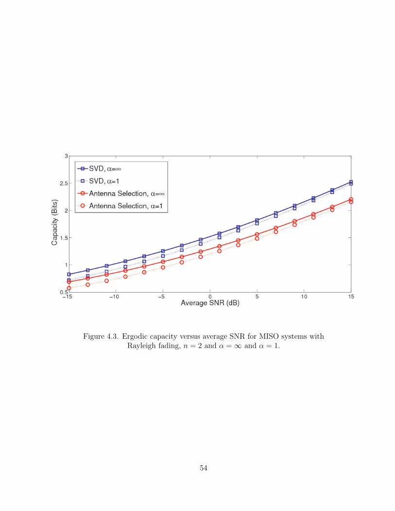
Figure 4.3. Ergodic capacity versus average SNR for MISO systems withRayleigh fading, n = 2 and α =∞ and α = 1.

54

words, if P ≤ Pmax, the difference between the capacity obtained from the optimal

power allocation policy subject to the long-term power constraint only and the one

obtained from the optimal power allocation subject to both long- and short-term

power constraints is relatively small (about 3 dB at low SNR and 1 dB at higher

SNR for the MISO systems with n = 2).

4.2.2 MIMO

we present some numerical results for MIMO systems with Rayleigh fading.

Figure 4.4 shows the value of αmax versus the average SNR per parallel channel

(λ = PmN0

) for 2 × 2 and 4 × 4 MIMO systems. This plot suggests similar ob-

servations as for MISO systems: for large average SNRs, αmax approaches unity,

and as the number of antennas increases, the value of αmax decreases, which is

desirable in practice. Intuitively, water-filling has more short-term fluctuations at

low SNR, which makes αmax larger. In fact, the short-term power constraint is

more relevant at low SNR compared to high SNR.

Figure 4.5 examines the effect of Pmax on the capacity of MIMO systems with

Rayleigh fading. We compare the capacity of two extreme cases: Pmax = P and

Pmax → ∞ (or α = 1 and α → ∞ with α defined in Section 3.3.1). The figure

shows the capacity versus average SNR for these two cases in a 2×2 MIMO system

along with the case of having CSI only at the receiver but not at the transmitter.

Note that this figure also examines the effect of P on the capacity if we consider

two extreme cases: P = P /m and P →∞ (or α = 1 and α→∞ with α defined

in Section 3.3.2). For other values of 1 < α < ∞ between the two extremes, the

capacity versus average SNR curve lies between the first two curves in Figure 4.5.

As we can see, the difference between the first two curves appears negligible.

55

Figure 4.4. The value of αmax, the threshold separating Cases 2 and 3,versus Average SNR per parallel channel ( P

mN0) for MIMO systems with

Rayleigh fading.

56

Figure 4.5. Ergodic capacity versus average SNR per parallel channel( PmN0

) for 2× 2 MIMO systems with Rayleigh fading.

57

The same result is reported in [24], in which the curves for the two cases of space-

time water-filling and spatial water-filling are equivalent to the case with α =∞

and α = 1 in the figure, respectively. To interpret this, note that at each fixed

average SNR, the small difference between the first two curves in Figure 4.5 is

the difference between the ergodic capacities with a same average SNR, but with

two extreme possibilities when Pmax is equal to P and when the short-term power

constraint is removed (Pmax =∞). The ergodic capacity of the channel with the

same average SNR but with a short-term power constraint P < Pmax < ∞ has

a value between the two extreme cases. Therefore, for a fixed average SNR, the

value of the short-term power constraint has a very small effect on the ergodic

capacity as long as it is equal to or larger than the long-term power constraint.

Note that in the case of MISO systems in Figure 4.3, the Pmax has a considerable

effect on the ergodic capacity for low SNR regimes. However, for MIMO systems,

this effect is negligible for all plotted range of SNRs, since the performance of

the spatial water-filling (it happens when Pmax = P ) is very close to the one of

the space-time water-filling (it happens when we remove the short-term power

constraint or α =∞).

According to the above discussion, one might argue that if we use a constant

power allocation across the time, i.e., replacing the two long- and short-term

power constraints in (3.10) with a more stringent power constraint∑m

k=1 Pk ≤

P when P ≤ Pmax (or 1 ≤ α), then we would have almost the same ergodic

capacity as in the optimal power allocation in (3.11). This reasoning is in fact

true, but surprisingly, the complexity of computing the constant power allocation

across time is often more than that of the optimal one. In the optimal power

allocation (3.11), except for the threshold v, which needs to be pre-computed

58

offline, we need to compute the threshold β online only for some of the channel

realizations (when∑m

k=1

(1v− P

mλ′k

)+

> Pmax). However, in the constant power

allocation across the time, we need to compute a threshold online (the threshold

for the spatial water-filling) for each channel realization.

When there is no CSI at the transmitter, the capacity for a 2 × 2 Rayleigh

fading MIMO system is plotted in Figure 4.5 and is labeled as “Without CSIT”.

As we can see, we have approximately 3 dB gain if we have full CSI comparing

to the case of having CSI only at the receiver in the low SNR regime. However,

for high SNRs, the ergodic capacity is the same for the two cases. This always

happens for a m × m i.i.d. Rayleigh fading MIMO system as discussed in [29],

since at high SNR, the water-filling strategy allocates an equal amount of power

to all the spatial modes, as well as an equal amount of power over time, and that is

what the transmitter does when it does not have CSI [29]. This reasoning remains

true for a general m× n i.i.d. Rayleigh fading MIMO system with m ≤ n, which

is not the case in a MISO system.

We stress that the results and observations in this section are only applicable

to iid Rayleigh fading. By contrast, the effect of Pmax on the ergodic capacity

is considerable if the model is Rayleigh fading with log-normal shadowing. We

anticipate such a result based upon our observations in conjunction with results

in [24], in which the authors demonstrate that with log-normal shadowing, space-

time water-filling achieves significantly higher ergodic capacity than spatial water-

filling at low to moderate SNR regimes.

59

4.3 Summary

In this chapter, we specialized the problem of Chapter 3 to Rayleigh fading

model. We focused on the first scenario, which the input power is subject to long-

and short-term power constraints. we obtained some of the constants and thresh-

olds introduced in the power policies before. In fact, most of these constants are

a function of the distribution of the fading coefficients. We simplified the calcu-

lations needed to obtain the constants for SISO, MISO, and MIMO systems with

Rayleigh fading. In addition, numerical results suggested that for the Rayleigh

fading case, a short-term power constraint that is larger than a long-term power

constraint does not significantly impact the ergodic capacity of the channel.

We obtained simplified equations for the thresholds introduced in the power

allocation in the SISO and MISO systems with Rayleigh fading in Case 2 (αmax ≤

α) and Case 3 (1 < α ≤ αmax), which their general structures were discussed

in Chapter 3. In addition, we found the value of αmax, the threshold separating

Cases 2 and 3 in the power allocation structure for SISO, MISO with optimal

beamforming, MISO with antenna selection, and MIMO systems with Rayleigh

fading. Furthermore, we sketched this value versus average SNR for SISO, MISO,

and MIMO systems. From the numerical results, we concluded that water-filling

has more short-term fluctuations at low SNR, which makes αmax larger. In fact,

the short-term power constraint is more relevant at low SNR compared to high

SNR.

Finally, we sketched the ergodic capacity versus average SNR for MISO and

MIMO systems with Rayleigh fading for two extreme cases α = ∞ and α = 1,

and figured out that the difference for these two cases is very small, especially in

the high SNR regime, which suggests that a short-term power constraint that is

60

larger than a long-term power constraint has a small effect on the ergodic capacity

of the channel.

61

CHAPTER 5

HARD POWER CONSTRAINTS IN ENERGY HARVESTING SYSTEMS

In this chapter, after introducing the model and mathematically stating the

problem, we analyze the asymptotic behavior of the optimal rate policy and ob-

jective function and state and prove our main results. Then, we extend the work

to multiple access channels.

5.1 Model and Problem Statement

The system model is shown in Figure 5.1. The data arrives from a higher layer

application and waits in the data buffer until transmission. Harvested energy

becomes available in the energy buffer.

We assume a block-fading channel model in which the fading coefficient stays

fixed over each block ofN consecutive channel uses. The complex fading coefficient

during the mth block is denoted by Hm. The baseband equivalent discrete-time

input-output relationship in this channel model is

Ym = XmHm + Zm, (5.1)

where Xm, Ym, and Zm are complex vectors in CN denoting the channel inputs,

the channel outputs, and the additive noise which is complex circularly symmetric

62

Figure 5.1. System Model

Gaussian random vector independent of the fading coefficients with zero mean and

covariance matrix σ2I, respectively.

The number of bits arriving in the data buffer at time m is a random variable

denoted by Am with average A. The state of the data buffer, i.e., the number of

bits in the data buffer, at time m is indicated by Sm. Let the random variable Em

denote the amount of energy arriving into the energy buffer at time m, and the

random variable Eremm denote the state of the energy buffer at time m, i.e., the

amount of energy remaining in the energy buffer. We assume that each of the ran-

dom sequences {Hm}∞m=1, {Am}∞m=1, and {Em}∞m=1 are independent and identically

distributed (iid) and independent of each other, i.e., memoryless assumption.

Let µm denote the number of bits the transmitter decides to send at time m

based on all the available information at the transmitter. Let P (Hm, µm) be the

63

required transmission power during a block when the fading coefficient is Hm and

the transmitter chooses to reliably transmit µm bits. We assume that CSI and

the current state of the data and energy buffers are known to the transmitter and

receiver (since the receiver should find the rate policy based on this information).

Assuming that N is large and based on the mutual information model in [4],

µm/N = log

(1 +|Hm|2P (Hm, µm)

σ2

), (5.2)

and therefore,

P (Hm, µm) =σ2

|Hm|2(2µm/N − 1

). (5.3)

The state of the data buffer would update as

Sm+1 = Sm + Am+1 − µm, (5.4)

and the state of the energy buffer would update as

Eremm+1 = Eremm + Em+1 −σ2

|Hm|2(2µm/N − 1

). (5.5)

Note that each unit of time equals to a block of data of N consecutive channel

uses, and energy arrives at the beginning of each time interval. Therefore, energy

and power are equivalent in this formulation. Furthermore, note that (5.4) is valid

only if the the length of the data buffer is infinite. When it is finite and equal to

L, the state of the data buffer would update as

Sm+1 = min {Sm + Am+1 − µm, L}. (5.6)

64

We impose two constraints on the rate policy µm. The number of bits that the

transmitter decides to send cannot be more than the number of bits in the data

buffer at each time, i.e.,

µm ≤ Sm. (5.7)

Additionally, the amount of energy used to send data at each time cannot be

more than the amount of the energy in the energy buffer (energy constraints).

This enforces the constraint

µm ≤ N log

(1 +|Hm|2Eremm

σ2

). (5.8)

We state our objective function as an average data buffer cost as in [3]. Let

b(Sm) be the cost of the data buffer when there are Sm bits in the buffer. The

function we aim to minimize over all rate policies is

lim supk→∞

1

k

k∑m=1

E [b(Sm)] . (5.9)

We deal with two possible cost functions in this chapter. If we consider the

cost function

b(Sm) =

1 if Sm = L,

0 otherwise,

(5.10)

then with the data buffer update as in (5.6), the objective function defined in (5.9)

would be the probability that the length of the buffer is equal to L, i.e., the

probability of overflow. If we use the following cost function instead

b(Sm) =Sm

A, (5.11)

65

then by Little’s law, the objective function in (5.9) would be the expected time

average delay in the data buffer. Note that the average total delay experienced

by the data is the sum of the delay in the data buffer plus the time from when

each block of data leaves the data buffer until it is decoded. Since the later delay

is constant in our coding model, we only focus on the average delay in the buffer.

In general, minimizing (5.9) subject to (5.7) and (5.8) is a dynamic program-

ming problem. Using the techniques in [5], some properties of the optimal policies

can be shown. Under the memoryless assumption mentioned before, it can be

shown ([3], [5], and [10]) that under some additional constraints on the state

spaces, there exists an optimal stationary policy that is independent of time and

depends only on the current fading coefficient and the states of the data and

energy buffers. We denote this rate policy by µ(S,Erem,H) which indicates the

number of bits transmitted in the state (S,Erem,H). Additionally, under this rate

policy the sequence {(Sm,Am,Eremm ,Em,Hm)} forms a Markov chain.

We will assume that under every given stationary policy µ this Markov chain is

ergodic with a steady state distribution πµ(S,A,Erem,E,H) which represents the asymp-

totic distribution of (Sm,Am,Eremm ,Em,Hm) under policy µ [3]. Now by rewriting

the objective function (5.9) and the constraints (5.7) and (5.8), we can write the

optimization problem as

minµ(S,Erem,H)

E [b(S)] , (5.12)

subject to µ(S,Erem,H) ≤ S,

µ(S,Erem,H) ≤ N log

(1 +|H|2Erem

σ2

),

where the data buffer state is updated as (5.4) or (5.6), and the energy buffer

66

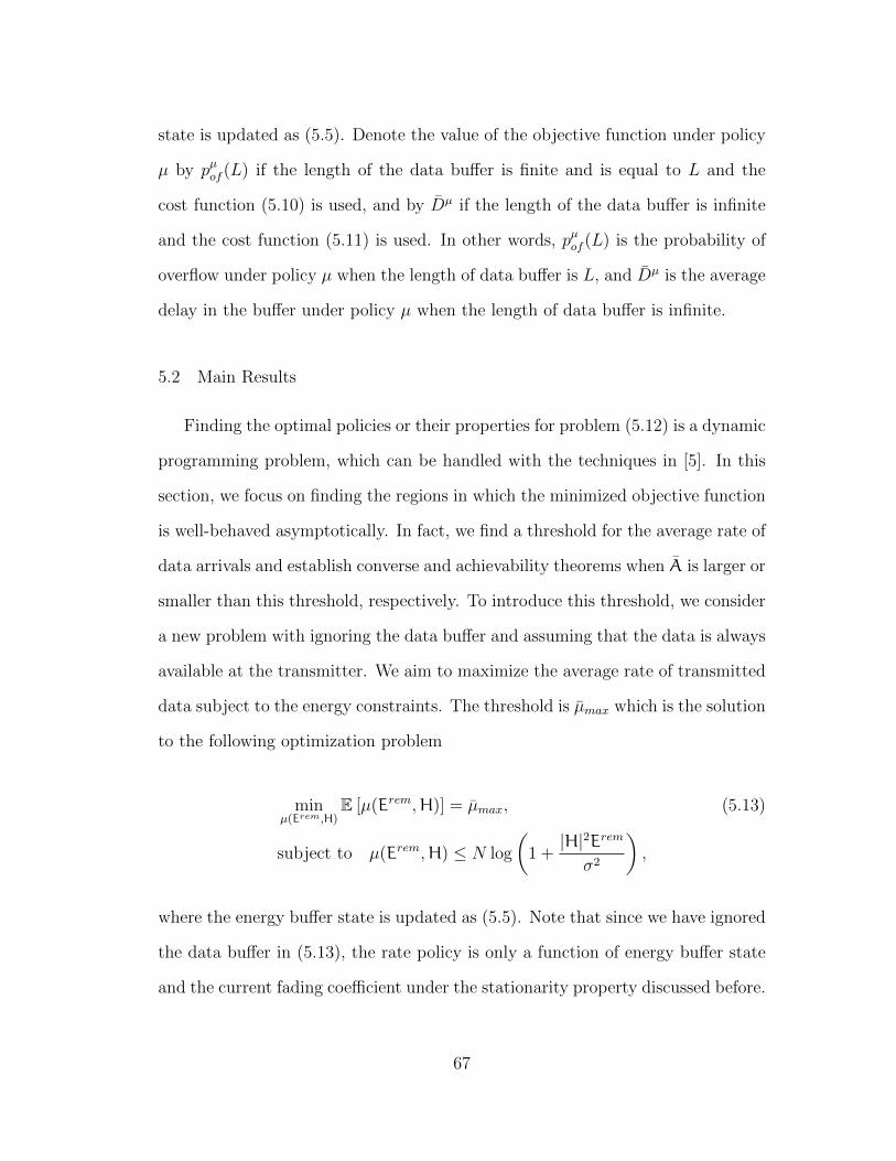
state is updated as (5.5). Denote the value of the objective function under policy

µ by pµof (L) if the length of the data buffer is finite and is equal to L and the

cost function (5.10) is used, and by Dµ if the length of the data buffer is infinite

and the cost function (5.11) is used. In other words, pµof (L) is the probability of

overflow under policy µ when the length of data buffer is L, and Dµ is the average

delay in the buffer under policy µ when the length of data buffer is infinite.

5.2 Main Results

Finding the optimal policies or their properties for problem (5.12) is a dynamic

programming problem, which can be handled with the techniques in [5]. In this

section, we focus on finding the regions in which the minimized objective function

is well-behaved asymptotically. In fact, we find a threshold for the average rate of

data arrivals and establish converse and achievability theorems when A is larger or

smaller than this threshold, respectively. To introduce this threshold, we consider

a new problem with ignoring the data buffer and assuming that the data is always

available at the transmitter. We aim to maximize the average rate of transmitted

data subject to the energy constraints. The threshold is µmax which is the solution

to the following optimization problem

minµ(Erem,H)

E [µ(Erem,H)] = µmax, (5.13)

subject to µ(Erem,H) ≤ N log

(1 +|H|2Erem

σ2

),

where the energy buffer state is updated as (5.5). Note that since we have ignored

the data buffer in (5.13), the rate policy is only a function of energy buffer state

and the current fading coefficient under the stationarity property discussed before.

67

Note that problem (5.13) is again a dynamic programming problem. This problem

is partially studied in [20], where some suboptimal power policies are derived. Now

we relate the solutions of problems (5.12) and (5.13) in Theorem 7 and Theorem 8

for minimum probability of overflow and minimum average delay, respectively. Let

Amax be the maximum value that the data arrival rate can take. In Theorem 7

and 8, let µmax be the optimal solution to (5.13).

Theorem 7. Assume that the length of the data buffer is finite and is equal to L

and the cost function (5.10) is used. If A > µmax, then pµof (L) ≥ A−µmaxAmax

under any

stationary policy µ that satisfies the constraints. On the other hand, if A < µmax,

then there exists a sequence of simple policies µL such that pµLof (L) = o( 1LK

) for

any K ≥ 2.

We call the first part of the theorem the converse part, and the second part

the achievability part.

Proof. Proof of the converse part: We define Fm := Am−µm and Gn :=∑n−1

m=1[Sm+

Am+1 − µm − L]+, where [x]+ := max (x, 0). Then, we have

Sn =n∑

m=1

Fm −Gn. (5.14)

By taking the expectation of the two sides of (5.14), dividing by n, and letting n

go to infinity, we have

limn→∞

1

nE [Sn] = lim

n→∞

1

n

n∑m=1

E [Fm]− limn→∞

1

nE [Gn] . (5.15)

Since the length of the data buffer is bounded, the left hand side of (5.15) equals to

zero. Because we have assumed that the Markov chain {(Sm,Am,Eremm ,Em,Hm)}

68

is ergodic under any stationary policy µ, and from (5.15) and definitions of Fm

and Gn, we have

E [A− µ] = E[[Sm + Am+1 − µm − L]+

]. (5.16)

Finally, we have

A− µmax ≤ (5.17a)

E [A− µ] = E[[Sm + Am+1 − µm − L]+

]≤ (5.17b)

AmaxE [b(S)] = Amaxpµof (L),

where (5.17a) comes from the fact that µmax ≥ E [µ] for any policy µ that satisfies

the energy constraints according to (5.13), and (5.17b) comes from the fact that

when the buffer overflows, Gn increases by at most Amax bits. Therefore, we can

conclude that pµof (L) ≥ A−µmaxAmax

.

Proof of the achievability part: We use the same simple policy as in [3]. That

is, we partition the data buffer state space into two disjoint sets [L/2, L] and

[0, L/2). Then we define the simple policy with drift vL as

µ(S,Erem,H) =

ψ1(Erem,H) if S ∈ [L/2, L],

ψ2(Erem,H) if S ∈ [0, L/2),

(5.18)

where E [ψ1(Erem,H)] = A+vL and E [ψ2(Erem,H)] = A−vL. The only difference

between this argument and the one in [3] is that we should make sure that these

policies are feasible with respect to the energy constraints. Note that we have

assumed that A < µmax. If we let vL =KVar[ψA(Erem,H)] lnL

L, where ψA(Erem,H) is

69

a policy with mean A, then limL→∞ vL = 0, and A + vL ≤ µmax as L→∞.

Therefore, both policies ψ1(Erem,H) and ψ2(Erem,H) are feasible, since a policy

with an average rate less than or equal to µmax is feasible according to (5.13), and

the asymptotic result proved in [3, Perposition 6.2.7] is also true here. That is

limL→∞ LKpµLof (L) = 0, i.e., pµLof (L) = o( 1

LK) for any K ≥ 2. Note that in our

problem we should use the results of Markov modulated random walks instead of

the properties of random walks discussed in [11].

The intuition behind the structure of the simple policy introduced for the

achievability part is that we do not want the data buffer to get too full or too

empty. On the one hand, the probability of overflow increases if the data buffer

is too full. On the other hand, we cannot take advantage of a good channel

coefficient or large amount of harvested energy to transmit enough data, if the

data buffer is too empty. Therefore, we increase the average rate of transmitted

data if the state of the data buffer is in the upper part, and decrease it if the state

of the data buffer is in the lower part.

Note that by choosing a large K, we can achieve the very fast convergence of

the probability of overflow to zero. However, as is discussed in [3], the problem

would be that the larger K is, the larger L will needed to be before the asymptotic

convergence rate is meaningful.

Theorem 8. Assume that the length of the data buffer is infinite and the cost

function (5.11) is used. If A > µmax, then the average delay Dµ is infinite under

any stationary policy µ that satisfies the constraints. On the other hand, if A <

µmax, then for every 0 ≤ v ≤ µmax− A there exists a simple policies µv defined as

70

µv(S,Erem,H) =

ψ1(Erem,H) if S ∈ [1/v,∞],

ψ2(Erem,H) if S ∈ [0, 1/v),

(5.19)

where E [ψ1(Erem,H)] = A+ v and E [ψ2(Erem,H)] = A− v, such that the average

delay can be upper bounded as

Dµv ≤ 1

vA+

exp (2vr∗(v))

r∗(v)A, (5.20)

where r∗(v) is the positive root of semi-invariant moment generating function [11]

of A− ψ1(Erem,H), i.e., the positive root of equation

E[exp

(r∗(v)(A− ψ1(Erem,H))

)]= 1. (5.21)

Proof. The proof of the first part (converse part): Let Fm := Am − µm, then we

have

Sn =n∑

m=1

Fm,

since overflow does not occur in this case. Therefore,

limn→∞

1

nE[Sn

A

]=

1

Alimn→∞

1

n

n∑m=1

E [Am − µm] .

Note that from the ergodicity property, we have

Dµ =

limn→∞

n(A− E [µ]) ≥ (5.22)

limn→∞

n(A− µmax) =∞, (5.23)

71

where (5.22) is because µmax is by definition the maximum value of the average

transmitted data under the hard power constraints, and (5.23) is because A >

µmax by assumption.

The proof of the second part (achievability part): Note that in the simple

policy (5.19), both policies ψ1(Erem,H) and ψ2(Erem,H) are feasible, since accord-

ing to (5.13) any policy with average rate less than µmax is feasible. Then, the

upper bound in (5.20) results from [3, Lemma 6.3.3] which uses some techniques

from [11] and [27].

Note that the achievability part of Theorem 8 introduces a set of upper bounds

for the average delay over which we can optimize.

5.3 Multiple Access: Separate and Cooperative Users

Similar to [3], we extend the results to multiple access channels with two users.

All the assumptions about the channel is the same as in the single user case. The

channel fading coefficients are indicated by Hm = (H1m,H

2m) at time m. Now,

we make some similar definitions as before. µm

:= (µ1m, µ

2m) is the rate policy,

Am := (A1m,A

2m) is a random vector indicates the number of bits arrive in the

data buffers with mean (A1, A2), and Sm := (S1m,S

2m) is the state of the data

buffers. When each of these come with an index m, it means at time m.

In this section, we assume that the data buffers have finite length L1 and L2

and let L := (L1, L2). The same assumptions and reasonings as in Section 5.1

about the stationarity of the rate policy and ergodicity of the Markov chain are

also valid here. We are interested in minimizing the average of a weighted function

of the probability of overflows, i.e., E [β1b(S1) + β1b(S1)], where b(Si), i = 1, 2 is

72

defined in a similar way as (5.10) with substituting L with Li, i = 1, 2 for the

first and second users, respectively. We have the same data buffer constraints as

in (5.7) for each user. Similar to (5.6), the update of the data buffers’ states can

be written in vector form as

Sm+1 = min {Sm + Am+1 − µm, L}. (5.24)

For convenience, we use the notation C(x) := log (1 + x/σ2). Let P 1 and

P 2 be the power (energy) that the first and the second users require to reliably

transmit µ1 and µ2 bits with fading coefficients H. We say that P := (P 1, P 2) is

in the feasible power region and show it by P ∈ P F (µ,H) when they satisfy the

constraints

|H1|2P 1 ≥ C−1

(µ1

N

), (5.25a)

|H2|2P 2 ≥ C−1

(µ2

N

), (5.25b)

|H1|2P 1 + |H2|2P 2 ≥ C−1

(µ1 + µ2

N

). (5.25c)

Figure 5.2 shows an example of this feasible region. We consider two situations,

when the energy buffers of the two users are separate, and when the energy is

harvested in a single battery (energy buffer). We call the former separate users

and the latter cooperative users.

5.3.1 Separate Users

We assume that there is a separate energy buffer for each user. E := (E1,E2) is

the amount of energy arrives in the energy buffers, and Erem := (Erem,1,Erem,2) is

73

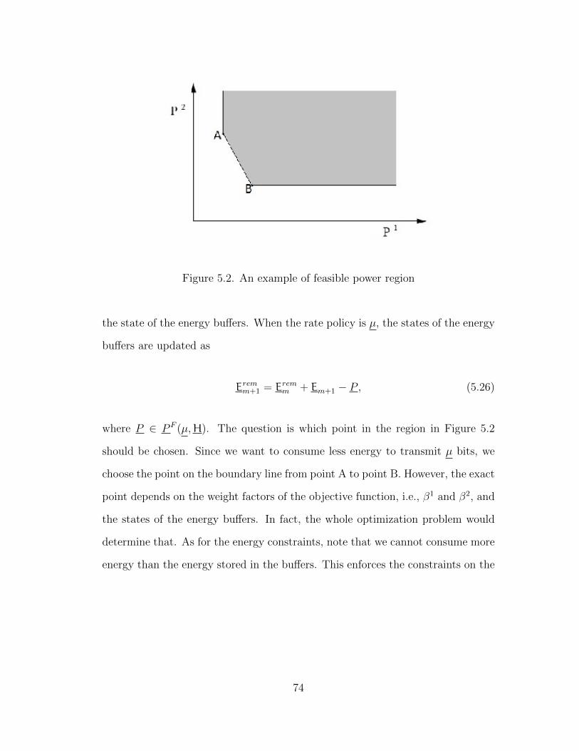
Figure 5.2. An example of feasible power region

the state of the energy buffers. When the rate policy is µ, the states of the energy

buffers are updated as

Eremm+1 = Eremm + Em+1 − P , (5.26)

where P ∈ P F (µ,H). The question is which point in the region in Figure 5.2

should be chosen. Since we want to consume less energy to transmit µ bits, we

choose the point on the boundary line from point A to point B. However, the exact

point depends on the weight factors of the objective function, i.e., β1 and β2, and

the states of the energy buffers. In fact, the whole optimization problem would

determine that. As for the energy constraints, note that we cannot consume more

energy than the energy stored in the buffers. This enforces the constraints on the

74

rate policy as

µ1 ≤ NC(|H1|2Erem,1), (5.27a)

µ2 ≤ NC(|H2|2Erem,2), (5.27b)

µ1 + µ2 ≤ NC(|H1|2Erem,1 + |H2|2Erem,2). (5.27c)

The problem is to minimize the objective function E [β1b(S1) + β1b(S1)] over all

policies µ under the described constraint.

As in Section 5.2, we are interested in finding the region for (A1, A2) such that

the minimized objective function is well-behaved asymptotically. To that end,

we consider the problem of transmitting as much data as possible subject to the

energy constraints when there are no data buffers and the data is always available

at each user. We say that the policy µ is allowable and show it by µ ∈ µA(Erem,H)

if it satisfies the energy constraints (5.27). Then, we define the average allowable

rate region as

µA :={E[µ(Erem,H)

]: µ(Erem,H) ∈ µA(Erem,H)

}, (5.28)

where the state of the energy buffers is updated as (5.26). In the following theorem

we assume that L1 = L and L2 = αL, where α is a finite constant. Let Aimax, i =

1, 2 be the maximum amount of data arrivals.

Theorem 9. If (A1, A2) /∈ µA, then for any stationary policy µ that satisfies

all the constraints, the probability of overflow is lower bounded by pµi

of ≥ (Ai −

E [µi])/Aimax, i = 1, 2, and at least for one of i = 1, 2 the right-hand side of this

inequality is greater than zero if the ranges of data arrivals are finite. On the

other hand, if (A1, A2) ∈ µA and it is not on the boundary region, then there

75

exists a sequence of simple policies µL

such that the probability of overflow has the

asymptotic behavior pµiLof = o( 1

LK), i = 1, 2 for any K ≥ 2.

The proof of this theorem uses the same techniques as in [3] and is similar to

the proof of previous two theorems.

5.3.2 Cooperative Users

In this section, we assume that the energy of both users is harvested in the

same energy buffer. This assumption is practical when the energy buffers of the

two users are allowed to cooperate. Let E := E1 + E2 be the amount of energy

arrives in the energy buffer, and Erem be the state of the energy buffer.

Since we consume the energy from the same energy buffer, only P 2 + P 2 is

important in the feasible power region. In other words, we want to minimize

P 1 + P 2 over all (P 1, P 2) ∈ P F (µ,H). Let P (µ,H) denote the solution to this

minimization problem. It can be easily shown that to minimize the sum power

P 1 +P 2, (P 1, P 2) should be the point A or B in figure 5.2 depending on which of

H1 or H2 is larger. The energy buffer state is updated as

Eremm+1 = Eremm + Em+1 − P (µ,H). (5.29)

The energy constraints are

µ1 ≤ NC(|H1|2Erem), (5.30a)

µ2 ≤ NC(|H2|2Erem), (5.30b)

µ1 + µ2 ≤ NC((|H1|2 + |H2|2)Erem), (5.30c)

and the objective function is the same as in Section 5.3.1. Again by ignoring

76

the data buffers and focusing on the energy constraints in the same way as in

Section 5.3.1, the allowable policies and average allowable rate region is defined

for cooperative users. Obviously, average allowable rate region for cooperative

users contains the one for separate users. How much they are different is out of

the scope of this Thesis. To best of our knowledge, this problem has not been

studied before and can be interesting. What is important here is that the same

theorem as Theorem 9 with the average allowable rate region for cooperative users

(µAcooperative

) is also valid here. We do not repeat stating the theorem.

Finally, note that for the multiple access channel, there is not a certain thresh-

old. Instead, we obtained an average allowable rate region and stated the theorem

with assumptions about the average arrival rates (A1, A2) belonging or not be-

longing to this region.

5.4 Summary

We mathematically formulated a wireless system in which data and energy

arrive randomly due to a data and energy random process and are stored in

the data and energy buffers. The objective is to spend the harvested energy

to transmit the stored data in such a way that a delay criterion, e.g., average

delay in the data buffer or probability of overflow, is minimized subject to the

hard power constraints imposed by the available energy. We characterized the

asymptotically optimal rate policies for such a system model, and proved some

converse and achievability theorems for both point-to-point channels and multiple

access channels with two users.

In particular, we showed that if the average rate of data arrival is larger than a

certain threshold, then the probability of overflow is lower bounded by a constant,

77

and the average delay is infinite if there is no constraint on the data buffer length.

On the other hand, if it is smaller than this threshold, then there exists a sequence

of simple policies such that the probability of overflow goes to zero faster than

1/LK for any K ≥ 2, where L is the length of the data buffer, and average delay

is upper bounded by some constants if there is no constraint on the data buffer

length. This threshold is the solution to a dynamic programming problem. Similar

results were obtained for the case of multiple access channels. We considered two

situations for the multiple access channels, when tho users have separate energy

buffers, and when they share a single energy buffer.

78

CHAPTER 6

CONCLUSION

6.1 Summary of Contributions

Resource allocation in wireless systems plays an important role in increasing

the efficiency of the systems by adaptively changing the rate or power of the

transmitter according to the channel fluctuations. In practice, complete or partial

channel state information at the transmitter makes this possible. In this work,

we assume that complete CSI is available at both the receiver and transmitter to

study the fundamental limits of the wireless systems, even though complete CSI

is an idealistic assumption in practical systems.

Generally, we are interested in optimizing a performance metric, e.g., maxi-

mizing the throughput or minimizing the delay of the system. However, practical

constrains are always imposed on real systems. In this thesis, we focused on power

and energy constraints imposed by applications, system design considerations, and

regulatory limitations. In particular, we considered long-term power constraints

to capture the life time of a rechargeable wireless device, short-term power con-

straints to model the regulations imposed by FCC, per-antenna power constraints

to avoid nonlinearity and distortion in the RF chains, and energy constraints (or

hard power constraints) to model the limitations in an energy harvesting systems.

In this thesis, we formulated optimization problems to derive the optimal power

and rate policies subject to the constraints discussed above. Once the system

79

was modeled and the objective functions and constraints were mathematically

formulated, we used different techniques from convex optimization theory and

stochastic processes to find the optimal power and rate policies. In the following

paragraphs, we summarize our results.

In Chapter 3, we derived the optimal power allocation in a fading environment

to maximize the ergodic capacity if the input power is subject to long- and short-

term power constraints for SISO and MIMO systems. Furthermore, we determined

a suboptimal power allocation if the input power is subject to long-term and

per-antenna power constraints and if the input power is subject to long-term,

short-term, and per-antenna power constraints in MIMO systems. We studied

the conditions for which one or more of the power constraints can essentially be

eliminated. In addition, we observed that the ratio of the power constraints plays

an important role in determining the optimal/suboptimal power allocation.

In Chapter 4, we specialized the problem of Chapter 3 to Rayleigh fading

models. We focused on the first scenario in which the input power is subject

to long- and short-term power constraints and obtained some of the constants

and thresholds introduced in the power policies in Chapter 3. In fact, most of

these constants are simply a function of the distribution of the fading coefficients.

We simplified the calculations needed to obtain the constants for SISO, MISO,

and MIMO systems with Rayleigh fading. In addition, numerical results suggested

that for the Rayleigh fading case, a short-term power constraint that is larger than

a long-term power constraint does not significantly impact the ergodic capacity of

the channel.

In Chapter 5, we mathematically formulated a model in which data and en-

ergy arrive randomly according to different arrival processes and are stored in data

80

and energy buffers. The objective is to spend the harvested energy to transmit

the stored data in such a way that a delay criterion, e.g., average delay in the

data buffer or probability of overflow, is minimized subject to the hard power

constraints imposed by the available energy. We characterized the asymptotically

optimal rate policies for such a system model, and proved some converse and

achievability theorems for both point-to-point channels and multiple access chan-

nels with two users. We considered two situations for the multiple access channels,

when tho users have separate energy buffers, and when they share a single energy

buffer.

6.2 Future Work

Many extensions can be pursued from the foundation of this thesis. In the

following, we motivate some important problems as extensions to different aspects

of our work. For each main chapter in this thesis, we introduce some extensions

in the context of that chapter.

For Chapter 3, we believe that following extensions are examples of possible

future work.

• Since we only considered point-to-point channels, this work can be natu-

rally extended to multiple access channels. However, the optimal power

policies for this situation are much more complex, since the ergodic sum

capacity formula, i.e., the objective function, is more involved and for each

user we should consider short-term, long-term and per-antenna power con-

straint, which increases the number of Lagrange multipliers and makes the

optimization problem much more intricate. We might also consider fairness

criteria for each user in multiple access channels. Another possible extension

81

is studying the broadcast channels. In this case, the objective function would

be even more complicated than the one for the multiple access channels.

• We have only focused on allocating power in time and space dimensions.

However, in frequency-selective fading channels with orthogonal frequency-

division multiplexing (OFDM) modulation, allocating power across frequency

also becomes important. In fact, this problem could be even more interest-

ing from a practical point of view, since it also allows capturing the FCC

constraints in a more general context, i.e., we can consider a spectral mask,

which is enforced by FCC, in our problem formulation.

• Complete CSI at both the receiver and transmitter was assumed in this

work. However, in practical systems, we may only have limited feedback and

therefore imperfect CSIT. Furthermore, CSI at the receiver could be noisy

due to the estimation error at the decoder. This motivates studying the

problem if only partial CSI is available at the receiver and/or transmitter.

In fact, in the LTE Advanced standard, only up to 8-bits of feedback is

allowed to report the Channel Quality Indicator (CQI) [23], which suggests

studying power allocations with these practical constraints.

For Chapter 4, we motivate the following extension.

• As we discussed, for the Rayleigh fading case, a short-term power constraint

that is larger than a long-term power constraint does not significantly impact

the ergodic capacity of the channel. It would be interesting to study other

fading models determine the properties of the fading distribution that lead

to this conclusion. For example, the effect of short-term power constraints

on the ergodic capacity is considerable if the model is Rayleigh fading with

82

log-normal shadowing as discussed in [24]. By studying other fading models,

such as Nakagami fading, Weibull fading, and Rician fading, we might infer

different conclusions about the role of each of the power constraints in the

optimal power allocation structure and in the resulting ergodic capacity.

Finally, in the context of Chapter 5, we suggest the following extensions.

• Our main result, which introduced a threshold and established converse and

achievability theorems if the average data arrival is larger or smaller than

this threshold, suggests studying the problem of determining this threshold.

It is in fact the maximum average rate that can be transmitted subject to

hard power constraints if we assume that there is always data waiting for

transmission at the encoder (or if there is no data buffer in the problem).

As we mentioned earlier, this is a dynamic programming problem and is

partially studied in [20] in which some suboptimal power policies are derived.

However, finding the properties of the optimal policy as well as determining

upper and lower bounds for the optimal solution to this problem in terms of

the average energy arrival rate would enable us to analyze the probability

of overflow or average delay in our main problem only based on the average

arrival data rate and average energy arrivals.

• Optimal policies: It is known that there is not a closed form solution to

dynamic programming problems. However, it is possible to characterize

some properties of the optimal policies. It is intuitive that the optimal

policy is non-decreasing in the state of energy buffers, in the state of the

data buffer, and in the current fading coefficient, i.e., the more energy in the

energy buffer, or the more bits in the data buffer, or the larger the channel

83

gain, the more bits that should be transmitted in the optimal policy. Proving

these intuitive observations can be considered as an important future work,

which will require some tools and techniques from dynamic programming

and optimal control.

Furthermore, it would be helpful to characterize the exact optimal policy in

a more simplified problem. As an example, consider the situation in which

energy arrivals, rate arrivals, and fading coefficients are binary, i.e., they can

be either zero or equal to a fixed amount, and the length of data buffer and

the capacity of energy buffer is finite. The exact solution to this simplified

problem could be helpful to figuring out the properties of the optimal power

policies for the general problem.

• We have considered two possibilities for the data buffer, with finite length

equal to L and without any constraint on the data buffer, but we did not

assume any constraint on the capacity of the energy buffer. In a realistic

situation, we are not able to harvest an infinite amount of energy. Studying

the same problem assuming that the capacity of the energy buffer is finite

can be another extension to this work.

• In the multiple access section, we observed that the average allowable rate

region for cooperative users contains the one for separate users. Obtain-

ing these two rate regions is again another dynamic programming problem.

Finding some outer and inner bounds for the difference of these two rate

regions can be done by using dynamic programming techniques. To the

best of our knowledge, this problem has not been studied before and can be

interesting as a possible future work.

84

BIBLIOGRAPHY

1. Federal Communictions Commission: Rules and Regulations, 2010. URLhttp://www.fcc.gov/oet/info/rules/.

2. M. S. Alouini and A. J. Goldsmith. Capacity of Rayleigh Fading Channelsunder Different Adaptive Transmission and Diversity-Combining Techniques.IEEE Transactions on Vehicular Technol, 48(4):1165–1181, 1999.

3. R. Berry. Power and Delay Trade-Offs in Fading Channels. PhD thesis, MIT,Cambridge, MA, 2000.

4. R. Berry and R. Gallager. Communication over Fading Channels with DelayConstraints. IEEE Transactions on Information Theory, 48(5):1135–1149,2002.

5. D. Bertsekas. Dynamic Programing and Optimal Control, vol. I and II. Bel-mont, MA: Athena Scientific, 1995.

6. S. Boyd and L. Vandenberghe. Convex Optimization. Cambridge, U.K.: Cam-bridge Univ. Press, 2004.

7. G. Caire, G. Taricco, and E. Biglieri. Optimum Power Control over FadingChannels. IEEE Transactions on Information Theory, 45(5):1468–1489, 1999.

8. R. R. Chen and Y. Lin. Optimal Power Control for Multiple Access Chan-nel with Peak and Average Power Constraints. In Proceedings of IEEE In-ternational Conference on Wireless Networks, Communications and MobileComputing, pages 1407–1411, 2005.

9. A. Feiten, R. Mathar, and S. Hanly. Eigenvalue-Based Optimum-Power Al-location for Gaussian Vector Channels. IEEE Transactions on InformationTheory, 53(6):2304–2309, 2007.

10. W. Feller. An Introduction To Probability Theory and Its Applications, vol.2. Wiley, New York, 1957.

11. R. Gallager. Discrete Stochastic Processes. Kluwer Academic Publishers,Boston, 1996.

85

12. A. Goldsmith, S. A. Jafar, N. Jindal, and S. Vishwanath. Capacity Limits ofMIMO Channels. IEEE Journal on Selected Area in Communications, 21(5):684–702, 2003.

13. A. J. Goldsmith and P. P. Varaiya. Capacity of Fading Channels with ChannelSide Information. IEEE Transactions on Information Theory, 43(6):1986–1992, 1997.

14. B. M. Hochwald and L. M. A. Jalloul. Statistical Distributions That Arise inConstrained Beamforming with Incomplete Channel Information. In Proceed-ings of IEEE Information Theory and Applications Workshop (ITA), pages1–10. San Diego, CA, USA, 2010.

15. S. K. Jayaweera and H. V. Poor. Capacity of Multiple-Antenna Systems withBoth Receiver and Transmitter Channel State Information. IEEE Transac-tions on Information Theory, 49(10):2697–2709, 2003.

16. M. A. Khojastepour and B. Aazhang. The Capacity of Average and PeakPower Constrainted Fading Channels with Channel Side Information. InProceedings of IEEE Wireless Cotnitnnications and Networking Conference(WCNC), pages 77–82, 2004.

17. R. Knopp and P. Humblet. Information Capacity and Power Control in Single-Cell Multiuser Communications. In Proceedings of IEEE International Con-ference on Communications (ICC), pages 331–335. Seattle, WA , USA, 1995.

18. A. W. Marshall and I. Olkin. Theory of Majorization and Its Applications.New York: Academic, 1979.

19. S. Musy and E. Telatar. On the Transmission of Bursty Sources. In Proceedingsof IEEE International Symposium On Information Theory (ISIT’06), pages2899–2903. Seattle, WA, USA, 2006.

20. O. Ozel, K. Tutuncuoglu, J. Yang, S. Ulukus, and A. Yener. Adaptive Trans-mission Policies for Energy Harvesting Nodes in Fading Channels. In Con-ference on Information Sciences and Systems (CISS). Baltimore, MD, USA,2011.

21. D. P. Palomar. Unified Framework for Linear MIMO Transceivers with Shap-ing Constraints. IEEE Communication Letters, 8(12):697–699, 2004.

22. R. Rajesh and V. Sharma. Capacity of fading gaussian chan-nel with an energy harvesting sensor node. Available online athttp://arxiv.org/PS cache/arxiv/pdf/1010/1010.5416v1.pdf.

86

23. S. Sesia, I. Toufik, and M. Baker. LTE: The UMTS Long Term Evolution.John Wiley and Sons, 2009.

24. Z. Shen, R. W. Heath, J. G. Andrews, and B. L. Evans. Comparison of Space-Time Water-filling and Spatial Water-filling for MIMO Fading Channels.In Proceedings of IEEE Global Telecommunications Conference (GLOBE-COM’04), pages 431–435, 2004.

25. E. Telatar. Capacity of Multi-Antenna Gaussian Channels. Eur. Trans.Telecomm. ETT, 10(6):585–596, 1999.

26. E. Telatar and R. Gallager. Combining queueing theory with informationtheory for multiaccess. IEEE Journal on Selected Areas in Communications,13(6):963–969, 1995.

27. D. Tse. Variable-rate Lossy Compression and its Effects on CommunicationNetworks. PhD thesis, MIT, Cambridge, MA, 1994.

28. D. Tse and S. Hanly. Multiaccess Fading Channels-Part I: Polymatroid Struc-ture, Optimal Resource Allocation and Throughput Capacities. IEEE Trans-actions on Information Theory, 44(7):2796–2815, 1998.

29. D. N. C. Tse and P. Viswanath. Fundamentals of Wireless Communications.Cambridge, U.K.: Cambridge Univ. Press, 2005.

30. J. Yang and S. Ulukus. Optimal packet scheduling in an en-ergy harvesting communication system. submitted to IEEETransactions on Communications, June 2010, available athttp://www.ece.umd.edu/ ulukus/papers/journal/opt-sch-ener-harv.pdf.

This document was prepared & typeset with pdfLATEX, and formatted withnddiss2ε classfile (v3.0[2005/07/27]) provided by Sameer Vijay.

87