Embed Size (px)
Citation preview

Optimal design of long-span steel portal frames using fabricatedbeams
McKinstray, R., Lim, J. B. P., Tanyimboh, T. T., Phan, D. T., & Sha, W. (2015). Optimal design of long-span steelportal frames using fabricated beams. Journal of Constructional Steel Research, 104, 104–114.https://doi.org/10.1016/j.jcsr.2014.10.010
Published in:Journal of Constructional Steel Research
Document Version:Peer reviewed version
Queen's University Belfast - Research Portal:Link to publication record in Queen's University Belfast Research Portal
Publisher rights© 2015, Elsevier. Licensed under the Creative Commons Attribution-NonCommercial-NoDerivatives 4.0 Internationalhttp://creativecommons.org/licenses/by-nc-nd/4.0/ which permits distribution and reproduction for non-commercial purposes, provided theauthor and source are cited.
General rightsCopyright for the publications made accessible via the Queen's University Belfast Research Portal is retained by the author(s) and / or othercopyright owners and it is a condition of accessing these publications that users recognise and abide by the legal requirements associatedwith these rights.
Take down policyThe Research Portal is Queen's institutional repository that provides access to Queen's research output. Every effort has been made toensure that content in the Research Portal does not infringe any person's rights, or applicable UK laws. If you discover content in theResearch Portal that you believe breaches copyright or violates any law, please contact [email protected].
Download date:26. Mar. 2020

1
Optimal design of long‐span steel portal frames using fabricated
beams
Ross McKinstray, James B.P. Lim, Tiku T. Tanyimboh, Duoc T. Phan, Wei Sha*
* Corresponding author
Ross McKinstray: SPACE, David Keir Building, Queen's University, Belfast, BT9 5AG, UK
Email: [email protected]
James B.P. Lim: SPACE, David Keir Building, Queen's University, Belfast, BT9 5AG, UK. Email:
Tiku T. Tanyimboh: Department of Civil and Environmental Engineering, University of
Strathclyde, Glasgow, G1 1XJ, UK. Email: [email protected]
Duoc T. Phan: Department of Civil Engineering, Universiti Tunku Abdul Rahman, Kuala
Lumpur, 53300, Malaysia. Email: [email protected]
Wei Sha: SPACE, David Keir Building, Queen's University, Belfast, BT9 5AG, UK. Email:
Ross McKinstray, PhD student
James B.P. Lim: PhD, Lecturer
Tiku T. Tanyimboh: PhD, Senior Lecturer
Duoc T. Phan: PhD, Assistant Professor
Wei Sha: PhD, Professor

2
Optimal design of long‐span steel portal frames using fabricated
beams
Abstract
This paper considers the optimal design of fabricated steel beams for long‐span portal
frames. The design optimisation takes into account ultimate as well as serviceability limit
states, adopting deflection limits recommended by the Steel Construction Institute (SCI).
Results for three benchmark frames demonstrate the efficiency of the optimisation
methodology. A genetic algorithm (GA) was used to optimise the dimensions of the plates
used for the columns, rafters and haunches. Discrete decision variables were adopted for
the thickness of the steel plates and continuous variables for the breadth and depth of the
plates. Strategies were developed to enhance the performance of the GA including solution
space reduction and a hybrid initial population half of which is derived using Latin
hypercube sampling. The results show the proposed GA‐based optimisation model
generates optimal and near‐optimal solutions consistently. A parametric study is then
conducted on frames of different spans. A significant variation in weight between fabricated
and conventional hot‐rolled steel portal frames is shown; for a 50 m span frame, a 14‐19%
saving in weight was achieved. Furthermore, since Universal Beam sections in the UK come
from a discrete section library, the results could also provide overall dimensions of other
beams that could be more efficient for portal frames. Eurocode 3 was used for illustrative
purposes; any alternative code of practice may be used.
Keywords: hot‐rolled steel; fabricated beams; portal frames; genetic algorithms;
serviceability limits; buckling limits

3
1 Introduction
In the UK, it is estimated that steel portal frames account for 90% of all single‐storey
buildings [1]. The vast majority of portal frames use hot‐rolled steel sections for the column
and rafter members. Using such sections, frames economically achieve spans of up to 50 m
[2].
For longer span frames, an alternative to the use of hot‐rolled steel sections could be
fabricated steel beam sections [3], [4]. Such fabricated beams, built‐up through the welding
of steel plates, have become increasingly popular for multi‐storey buildings, where clear
spans of up to 100 m are achievable [1]. In this paper, the use of such fabricated beams for
portal frames will be considered using a genetic algorithm (GA) to size the dimensions of the
fabricated beams.
Genetic algorithms have previously been applied to the design optimisation of hot‐rolled
steel portal frames [5]–[8]. In these studies, only four design variables were used; namely,
the cross‐section sizes of the columns and rafters, and the length and depth of the eaves
haunch [8]. The design used in this present paper was elastic. Phan et al. [8] showed that
elastic design was sufficient since the design was controlled by deflection limits.
On the other hand, a design optimisation of fabricated steel sections can involve up to
thirteen design variables (see Section 2.2); these being, the dimensions of the plates of each
of the members as well as the dimensions of the haunch. To reduce the number of function
evaluations, an effective means of enhancing the reliability is required.
Three benchmark frames are considered, with the frames designed elastically under gravity
load in accordance with Eurocode 3. Both ultimate and serviceability limit states are
considered. A parametric study is conducted to explore the full search space for single story
steel buildings. Spans of 14 m to 50 m and eave heights varying from 4 m to 12 m were
considered.
2 Benchmarkframes
Three frames are considered:
Frame A: Span of 40 m and height of 10 m

4
Frame B: Span of 50 m and height of 12 m
Frame C: Span of 60 m and height of 12 m
The pitch and frame spacing for all three frames are 6o and 6 m, respectively; such a pitch
and frame spacing are typical for portal frames in the UK [2]. The column bases are assumed
to be pinned. It is also assumed that the steel sections are fabricated from S275 steel [9].
2.1 Portalframescomposedofuniversalbeams
Frames are generated by selecting universal beam sections for the column and rafters from
a list of 80 standard sections given in the SCI “Steel building design: Design data” Book [10].
The column, rafter and haunch sections are considered as discrete variables with haunch
length (HL) treated as a continuous variable [8].
Four universal beam cases (UBC) are considered:
UBC1 has two decision variables: the column and rafter sections. The haunch is
assumed to be the same as the rafter section and haunch length is fixed at 10% of
the span
UBC2 has three decision variables: column, rafter and haunch sections. The haunch
length is fixed at 10% of the span
UBC3 also has three decision variables: column section, rafter section and haunch
length. The haunch is assumed to be the same as the rafter section.
UBC4 has four decision variables: column section, rafter section, haunch section and
haunch length.
2.2 Portalframescomposedoffabricatedbeams
Portal frames composed of fabricated beams are generated with the dimensions described
below. The plate thickness is treated as discrete variables and used for the web and flange.
34 plate thicknesses available within the UK are considered; at 1 mm spacings 6‐25 mm; 5
mm spacings 30‐80 mm and individually 12.5, 28 and 63.5 mm. The depths and breadths of
the sections are treated as continuous variables with a range of 110 mm to 2000 mm and 50
mm to 600 mm, respectively.
Three Fabricated Beam Cases (FBC) are considered as follows with 13 decision variables in
total: hC, hR, hH, bC, bR, bH, twC, twR, twH, tfC, tfR, tfH, and HL. The notations use standard

5
(descriptive) terminology: h for height, b for breadth and t for thickness, including web (w in
subscript) and flange (f in subscript) thicknesses; in subscript, C for column, R for rafter and
H for haunch.
FBC1 is defined as follows: hC, hR = hH, bC = bR = bH, twC = twR = twH, tfC = tfR = tfH, and HL. FBC1
also has 13 decision variables that are further constrained as shown in the equations.
FBC2 has the following properties: hC, hR = hH, bC, bR = bH, twC, twR = twH, tfC, tfR = tfH, and HL.
Using restrictions for FBC1 and FBC2 corresponds to the operational simplicity and possibly
economy of using a smaller numbers of plate sizes.
FBC3 has the following properties: hC, hR, hH, bC, bR, bH, twC, twR, twH, tfC, tfR, tfH, and HL.
In addition, discussions with manufacturers of fabricated beams suggest that the following
geometric constraints are required in order to ensure that the plates can be welded and
handled practically on the fabrication shop floor:
hC > 3tfC; hR > 3tfR; hH > 3tfH
tfC > twC; tfR > twR; tfH > twH.
3 Frameactions
In this paper, the permanent actions (G) and variable actions (Q) assumed to act on the
frames are as follows:
G: 0.55 kN/m2 + self‐weight of primary steel members
Q: 0.60 kN/m2
Under vertical load, the frame should be verified at the ultimate and serviceability limit
where the deflection limits and actions combination as recommended by the SCI [8,11] are
adopted. Variable and permanent actions are factored in accordance with Eurocode 3:
Design of steel structures [12]:
ULS = 1.35G + 1.5Q
SLS1 = 1.0G + 1.0Q (for absolute deflection)

6
SLS2 = 1.0Q (for differential deflection relative to adjacent frame)
where,
ULS is the ultimate limit state
SLS is the serviceability limit state
4 Ultimatelimitstatedesign
4.1 Elasticframeanalysis
Modern practice has shown that plastic design produces the most efficient designs in the
majority of cases [2], [13]. Elastic design is still used, particularly when serviceability limit
state deflections will control frame design [14], [15]. Phan et al. [8] have demonstrated that,
if the SCI deflection limits are adopted, serviceability limit states control design. Therefore,
elastic design is used in this paper.
A frame analysis program, written by the authors in MATLAB, was used for the purpose of
the elastic frame analysis. The internal forces, namely, axial forces, shear forces, and
bending moments can be calculated at any point within the frame. It should be noted that
second‐order effects are not considered, since the geometry in the benchmark frames
satisfy the requirements for in‐plane stability of the sway check method, described in BS
5950 [16].
4.2 Ultimatelimitstatedesignrequirements
Structural members are designed to satisfy the requirements for local capacity in
accordance with Eurocode 3 [17]. Specifically, members are verified for capacity under
shear, axial, and moment, and combined moment and axial force. For fabricated beams, the
buckling curves used are taken in accordance with the UK National Annex [18]. Sections are
classified based on the axial and bending force in conjunction with their geometric
properties as class 1, 2 or 3. For class 1 or 2 sections, a plastic design approach is used in
verification. For class 3 sections an elastic verification is substituted in the design. Sections
outside this range (class 4) are excluded through use of a GA penalty.

7
Local buckling verifications are excluded under the proviso that a more detailed design of
any necessary web and flange stiffeners will be conducted on the optimum selected
sections. For example the stiffeners are generally required in the eave connections to allow
for the concentrated axial forces transference from the rafter to the column.
4.2.1 ShearcapacityThe shear force, VEd, should not be greater than the shear capacity, Vc,Rd.
V V , (1)
The shear capacity is given by:
V , /√
(2)
where
fy is the yield stress of steel
Av is the shear area
γ is partial factor for resistance
V , is the shear design resistance for class 1, 2 and 3 sections
4.2.2 AxialcapacityThe axial capacity should be verified to ensure that the axial force NEd does not exceed the
axial capacity (NRd) of the member.
N N , (3)
4.2.3 MomentcapacityThe bending moment should not be larger than the moment capacity of the cross section,
Mc,Rd.
M M , (4)
where
MEd is the moment applied to the critical section

8
For class 1 or 2 sections M , is the plastic design resistance of the
section, M ,
For class 3 sections M , is the elastic design resistance of the
section, M ,
When members are subject to both compression and bending, the moment capacity M ,
is reduced if the axial force is significant in accordance with clause 6.2.9.1 for class 1 or 2
sections and check 6.2.9.2 for class 3 within Eurocode 3 Part 1‐1 [17].
4.2.4 BucklingBuckling is verified using equations 6.61 and 6.62 of Eurocode 3 [17]. As the frame is under
single axis bending the additional second axis bending terms can be removed resulting in
equation 5 and 6 below [19].
01,
,
,,
Rdb
Edyzy
Rdzb
Ed
M
Mk
N
N (5)
(6)
The equivalent uniform moment factors kzy and kyy interaction factors are calculated based
on the Annex B method of Eurocode 3 [17]. Lateral restraint is provided by the side rails and
purlins; torsional restraint is provided by the addition of stays to the bottom flange. Purlin
and side rail spacing (Lcr) is generally controlled by the spanning capability of the cladding,
normally 1 to 3 m depending on the loading. The rafter buckling is considered in zone C of
Figure 1 and the column is verified equally at the column top (see Figure 2). In both cases a
specified Lcr restraint spacing is used in the calculation of stability based unity factors. In this
paper feasible cladding spans of 1.5 m and 3 m are considered. Elsewhere in the frame
where Lateral Torsional Buckling (LTB) is not explicitly considered it is assumed that
restraints are provided at the necessary spacing to provide adequate stability.
4.2.5 ShearBucklingThe shear buckling check has been considered and was found not to control the design,
based on unstiffened webs with non‐rigid end posts verified, in accordance with EN‐1993‐1‐
5:2006 [20], with transverse stiffeners provided at the support and at the connections. The
01,
,
,,
Rdb
Edyyy
Rdyb
Ed
M
Mk
N
N

9
maximum observed reduction in shear force design capacity was 40%, with an average
reduction of 26.5% for the FC2 cases.
5 Optimisationmodel
The objective of the overall design optimisation is to determine the portal frame with
the minimum primary member steel material weight, whilst satisfying the design
requirements. The weight of the frame depends on the cross‐section sizes of members. The
objective function is expressed in terms of the weight of the primary members per square
metre of the floor area. The weight was calculated by summation of the volume of steel
material throughout the frame using element lengths and cross‐sectional areas.
The design constraints unity factors are as follows:
1.
1 Rdc
Ed
V
Vg (7a)
12 Rd
Ed
N
Ng (7b)
1.
3 Rdc
Ed
M
Mg (7c)
1,
,
,,4
Rdb
Edyzy
Rdzb
Ed
M
Mk
N
Ng (7d)
(7e)
(7f)
(7g)
1.2if3t 0Otherwise
(7h)
1,
,
,,5
Rdb
Edyyy
Rdyb
Ed
M
Mk
N
Ng
16 ue
eg
17 ua
ag
10
1.2ift t 0Otherwise
(7i)
1.2ifclass40Otherwise
(7j)
where δe and δa = deflections at eaves and apex, respectively. The superscript u indicates
the maximum permissible deflection. The constraints for ultimate limit state design are g1 to
g5 while the serviceability limit state design constraints are g6 and g7. Constraint g1 is for
shear capacity; g2 is for axial capacity; g3 is for combined axial and bending capacity; g4 and
g5 are interaction of axial force and bending moment on buckling for major axis; and g6 and
g7 are for horizontal and vertical deflection limits. If the geometrical cross‐section
constraints, g8, g9 and g10, is exceeded, an arbitrary (lowest tier) unity factor of 1.2 is
assigned. These are verified throughout the frame and are further denoted to show the
maximum value within a given zone: gxC within the column; gxR within the rafter; gxH within
the haunch.
6 Optimisationmethodology
The design optimisation considered in this paper contains mixed discrete and continuous
design variables. This was implemented using a genetic algorithm within the optimisation
toolbox in MATLAB. In order to consider discrete and continuous design variables, special
crossover and mutation functions enforce variables to be integers [21]. One of the benefits
of a real coded genetic algorithm is that genetic operators are directly applied to the design
variables without coding and decoding as with binary string GAs. As demonstrated by Deb
[22] real coded GA is appropriate for optimisation problems having continuous design
variables. This allowed for the representation of the frame using realistic parameters that
can be used directly in design.
It has been identified that genetic algorithms sometimes prematurely converge to a local
optimum solution due to the domination of superior solutions in the current population
[23], [24]. It has also been observed that using the real coded genetic algorithms, large
population sizes are needed in order to obtain the optimum solution consistently [25].
11
6.1 Geneticalgorithmconfiguration
Two techniques were explored in order to improve reliability and speed of convergence
both applied prior to starting the GA. The first method is Search Space Reduction (SSR).
Impressive reductions in GA execution times have been demonstrated recently. For
example, Kadu et al. [26] used heuristics to limit the GA search to a region of the solution
space in which near optimal solutions were thought to exist. Known constraint violations
were used to maximise the proportion of feasible solutions even with geometric changes.
This was done by initially calculating the frame bending moments using the maximum
available sections then eliminating sections with significant lower moment capacities for
both the column and rafter independently. This would reduce the number of sections
considered from 80 to approximately 30.
The second method is Improved Initial population (IIP) where the size of the initial
population was larger than subsequent generations ensuring that several viable solutions
were included in the first generation. The initial population was pre‐generated using a Latin
hypercube (LH) sampling plan. Two sizes of initial populations 6 and 12 times the standard
GA population size were considered. The larger initial population was then ranked based on
fitness value. The GA’s second generation was then generated with a population created
using 50% from the larger initial population’s best solutions and the rest randomly
throughout the available search space by the GA.
The optimisation was conducted on a workstation (2.53 GHz CPU, 4GB RAM). Quoted
computational times and function evaluation totals include the effort required in the phases
before moving to the genetic algorithm. An outline of the GA stages is presented in Figure 3.
Elite values are preserved 4 or 8 individuals, 4 for small populations and 8 for populations in
excess of 150 individuals. Selection is conducted using roulette selection.
Mutation of the variables was performed using an adaptive feasible approach where
mutation direction is based on the last successful or unsuccessful generation and the values
are kept within the bounds of the optimisation. Selected parents are then combined using a
scattered crossover operation where variables are converted to binary and the random bits
from each are combined [27].

12
The optimisation was stopped when the maximum number of generations is reached, set at
100‐250 generations. Additionally the optimisation was also terminated by convergence
defined as 50 generations with no improvement; a function tolerance of 10‐6 was specified.
The maximum number of generations required generally was less than the maximum with
almost all optimisations stops attributed to either the convergence criteria.
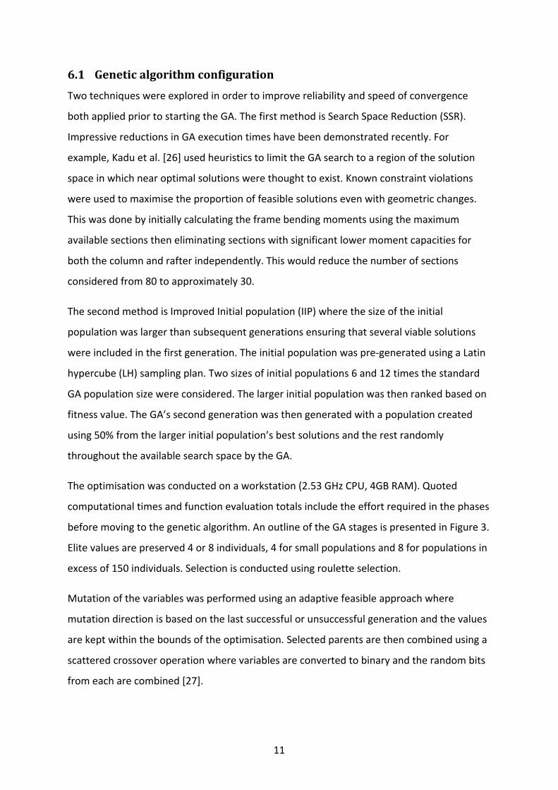
6.2 Fitnessandpenaltyfunctions
The objective of the optimisation is the minimum weight of the primary members of the
portal frame. This includes the weight of the column, rafter and haunch elements. For the
haunch sections, this weight includes any wastage in material as a result of the fabrication.
Figure 4 shows details of the cutting required for the section fabrication, with the white area
representing wasted material, and hH the additional depth achieved once the section has
been welded onto the rafter. The haunch sections are cut within the web outside the root
radius, realistically reflecting fabrication cutting conditions.
To solve the optimisation problem, a penalty based approach was added to the calculated
frame weight (Fweight), see Equation 8 to obtain the optimisation fitness value (Fp). Two levels
of violation were considered, the standard violation penalty (P) was a weight equivalent to
the heaviest available configuration used to eliminate moderate violations (maximum
constraint value under 1.5). For higher violations a penalty ten times the standard penalty
value was added. The maximum value of any individual unity factor (gM) outlined in Section
5 was used to determine the extent of any violation. It was observed that high penalty
values were required in order to eliminate very infeasible solutions. Otherwise the infeasible
solutions would undercut feasible solutions.
1 1 1.510 1.5
(8)

13
7 Resultsanddiscussion
7.1 Reliabilitystudy
For different numbers of design variables (based on optimisation case) different global
population sizes were investigated using a population based on a multiplier of 5, 10, 15, 20,
25 and 30 times the number of design variables with each optimisation run 30 times.
A total of 6 optimisation control strategies variations (see Table 1 and Table 2) were used,
for 7 different sets of optimisation design variables consisting of 4 Universal Beam Cases
(UBC) and 3 Fabricated Beam Cases (FBC). Table 1 includes the standard deviation, an
indication of the reliability of the optimisation for different GA configurations. Table 2
shows the required number of function evaluations for a given configuration to achieve the
reliability shown in Table 1. This totalled 252 variations per frame considered each run 30
times. A representative result is presented in Table 1 and Table 2 for Frame A using UBC3.
All of the optimisation cases (UBC1, UBC2…) produced comparable trends when switching
between optimisation control strategies. It is observed that for both search space reduction
and improved initial population, the standard deviation for small population multipliers is
reduced significantly. As the computational effort required (in terms of mean function
evaluations) increases, the standard deviation reduces to as low as 0.28 kg/m2.
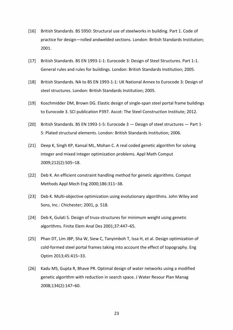
An example GA progress against function evaluations is shown in Figure 5 comparing the
performance of the standard GA with the enhancement methods SSR and IIP. Achieving the
global optimum for ×15 multiplier is rare without SSR or IIP. However it would appear that
local optimums are being found in the very near vicinity of the global optimum. From a
designer’s perspective, the additional effort required to achieve the global optimum,
outweighs the time required to run the simulation. Using SSR only results in a faster
convergence using less function evaluations due to a lower initial starting. Combining SSR
with an IIP of 12 times the standard population results in the GA starting from an even lower
starting fitness position but used more function evaluations. The increased number of
function evaluations was only marginal, with lower fitness more consistently found; it is
therefore useful for increasing reliability without disproportionately increasing optimisation
time. Similar observations can be seen in Table 2 where more results are presented for
comparison.

14
The use of SSR allows for faster optimum convergence reducing function evaluations with
the GA having a better starting position. IIP(×12) has similar but less obvious benefits than
simply increasing the global population multiplier. Increasing the global population
multiplier significantly increases the number of function evaluations due to the stopping
criteria in many cases being based on the number of stall generations. This will lead to
higher numbers of individuals in each of the stall generations making it less efficient than
using a combined SSR and IIP(×12) approach which only has a large population in the first
generation. It can also be seen IIP(×12) also has a similar effect of SSR where the first
generation will have a better starting position leading to a faster convergence.
7.2 Recommendedgeneticalgorithmconfiguration
From reviewing the 30 run study a population multiplier of 15 seems to have an effective
balance of reliability and computational effort. To further reduce the required
computational effort it was necessary to decrease the number of GA iterations per
optimisation run. As both reduction strategies allowed for lower optimum variation with
reduced computational effort it is recommended that both search space reduction (where
available) and an initial generation population multiplier of 12 is used (see bold numbers in
Table 1 and Table 2). In order to check that the reliability was not unacceptably adversely
affected a comparison is made between 10 and 30 runs (see Table 3).
The mean weight variation change from 30 GA runs to 10 runs is small indicating that 10
runs are sufficient for optimisation purposes. In general the optimum mean weight variation
is below 2% of the optimum weight using 10 runs. The exception is FBC3, where a higher
global population multiplier may be justified due to the larger number of interacting
variables. The efficiency could be further improved by reducing the stall generation stopping
constraint from 50 generations to 30, eliminating unnecessary function evaluations. This
was not implemented in this study as it would likely permit for faster convergence but with
sacrificed reliability.
It is therefore recommended that this configuration is used for fast reliable results with all
beam cases, with the exclusion of FBC3 where higher variations may be observed. It will be
shown in Section 7.5 that case FBC3 is not recommended. Therefore optimising the GA
configuration for FBC3 will not be explored further.

15
7.3 Comparisonofresultsagainstpreviouslyreportedinliterature
In order to validate the proposed modelling and optimisation method, a comparison is
made against results previously published in the literature. It should be noted that all the
examples in the literature are based on conventional hot‐rolled steel portal frames. As each
author calculated frame weight differently due to different geometric assumptions, a direct
weight comparison is therefore not possible; instead the optimum chosen sections are
compared.
In these comparisons it is assumed that the haunch would be fabricated i.e. the length and
breadth of their haunch could be of any size. In practice the haunch is usually cut from a
universal beam section (Figure 4) and this section is usually the same section as used for the
rafter. The cut shown in Figure 4 is practical but the previous authors did not do this
realistically. For the purposes of the comparisons described in this section, optimisation case
UBC3 is considered; it should be noted that UBC1 and 2 produce similar weights.
7.3.1 IssaandMohammadThe benchmark frame adopted by Issa & Mohammad [6], as presented by Saka [5], is
optimised. The frame considered is of span of 20 m, height to eaves of 5 m and pitch of
8.53o. The load acting on the frame is 4 kN/m vertical UDL acting globally on the rafter.
Issa and Mohammad adopted deflection limits of hf/300 and Lf/360 for the eaves and apex,
respectively, which are more stringent than the SCI deflection limits. It should be noted that
the deflection limits by Issa and Mohammad were verified at the same actions as the
member verification, i.e. no distinction was made for the actions between ultimate limit
state design and serviceability state for deflection verification. It should also be noted that
although the optimisation conducted by Issa and Mohammad included member buckling
effects, they reported in their paper that deflections limits governed this particular
benchmark design; the frame is therefore suitable for use as a benchmark for comparison.
Table 4 shows the results of the optimisation. It can be seen that the section sizes for the
column and rafter are the same as that of Phan et al. [8]. However, HL is longer than that of
Phan et al., since the haunch is assumed to be cut from the same section as the rafter.
7.3.2 SCIframe

16
The benchmark frame adopted by Phan et al. [8], based on an SCI worked example [2], is
also compared against the developed model. The frame geometry had a span of 30 m,
height to eaves of 7 m and pitch of 6o. The load acting on the frame is 11.3 kN/m vertical
UDL, comprised of 0.66 and 0.6 kN/m2 for permanent and variable actions, respectively,
with a frame spacing of 6 m. For the comparison, the loading factors and constraints were
altered to reflect the conditions reported. The SCI deflection limits were adopted.
The results of optimisation in comparison to Phan et al. are presented in Table 4. For UBC3
the same sections were selected as Phan et al. However, a longer HL was required. The cut
haunch used in UBC3 is more realistic given it prevalence in the industry but is still
comparable to Phan et al. results. The same primary members were selected under similar
loading conditions and the total steel volumes within the haunches are similar.
7.4 Portalframescomposedofuniversalbeams
In this section, the optimisation benchmark frames described in Section 2 are optimised
using the recommend GA configuration from Section 7.2. It should be noted that Frame C
span of 60 m was observed to be outside the range of UB based portal frames and therefore
was only optimised using fabricated beams.
The results of the universal beam optimisation are presented in Table 5. As the number of
design variables increase for both Frames A and B, the primary structural weight reduces. In
all cases, Eurocode capacity based moment verification dominates over others (shear and
axial based). The deflection at the apex is binding. Using universal beam sections LTB was
verified at both 1.5 m and 2.5 m restraint spacings (Lcr). For Frames A and B, LTB was found
not to be design controlling producing the same optimum results for both considered
lengths.
The largest weight savings were found to be achieved by including the haunch section as a
design variable within the GA. However, the sections selected tend to be significantly
different than the rafter and column sections.
7.5 Portalframescomposedoffabricatedbeams
Table 6 and Table 7 show the results of the portal frame optimisation composed of
fabricated beams with restraint spacings (Lcr) of 1.5 m and 2.5 m, respectively. For ease of

17
comparison, the dimensions of the fabricated beams are shown using the same designation
as for standard universal beams i.e. depth × breadth × weight (in kg/m).
It can be observed that the dimensions of the fabricated beams are controlled by both
deflections and buckling stability. In general the depth of the section is controlled by the
deflection of the frame while the breadth controls the stability. Comparing Table 6 and
Table 7, increasing the restraint spacing (Lcr) from 1.5 m to 2.5 m results in an average
optimum frame weight increase of 2.6%. This increase in optimum frame weight is due to
the additional steel needed to provide stability to the section.
The most proficient GA decision variable configuration was found to be FBC2 where the
haunch section is based on the rafter. When the haunch was allowed to vary independently
from the rafter (FBC3) the haunch could be very shallow or significantly out of proportion
with the rafter. This would produce the lightest frame weight but would make the
fabrication and joint detailing very difficult. A much better option is a configuration where
the haunch is based on the rafter (FBC2) resulting in a frame that can be fabricated more
easily, with a minimal frame weight increase of 1‐2% over the more optimum weight of
FBC3.
7.6 Observations
In all cases, portal frames composed of fabricated beams are lighter than those using
universal beams. Figure 6 compares the cross‐section of Frame A with UBC3 and FBC2
drawn to scale side by side. It can be seen that the fabricated beams tend to be deeper
generating the required moment capacity while sacrificing the inherent stability generally
found in a rolled section by increasing the depth and reducing the breadth.
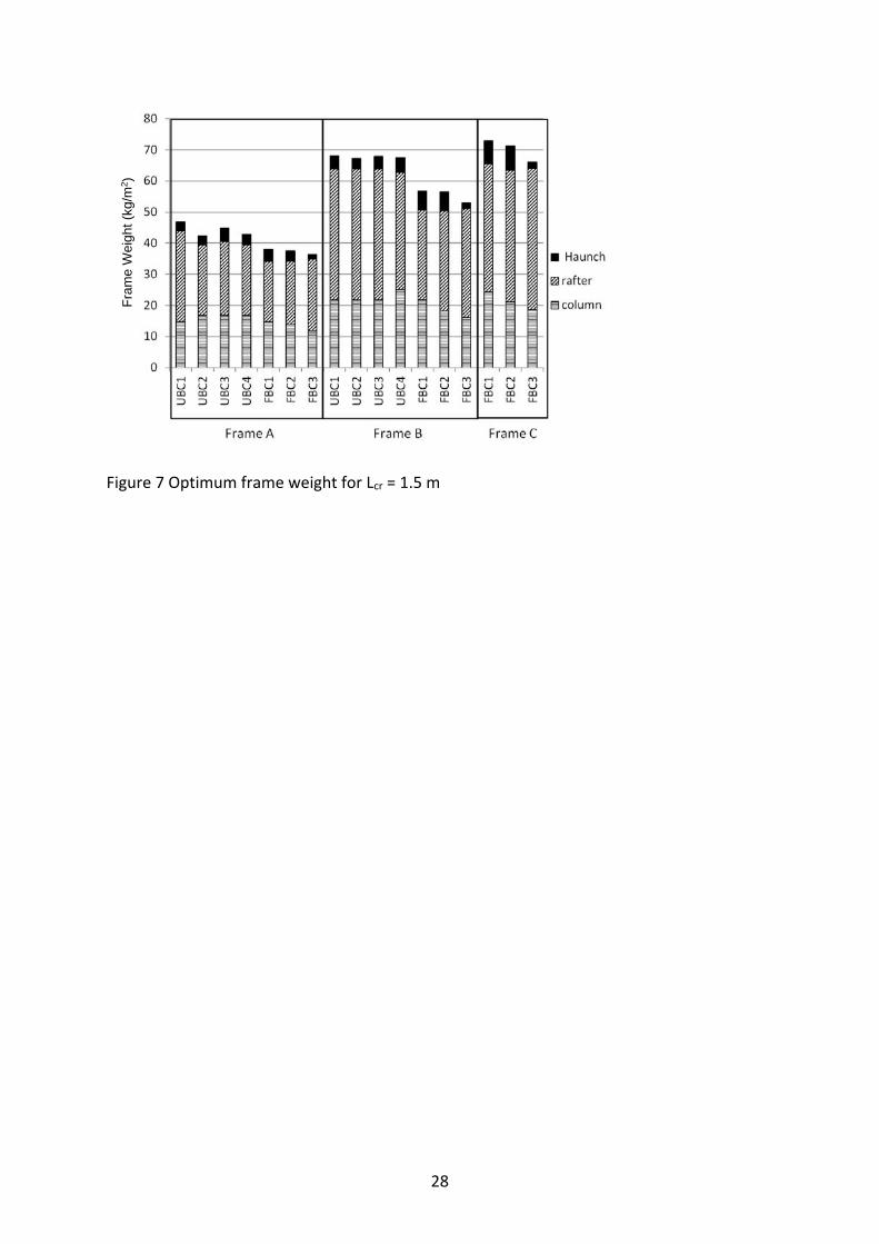
The change in sectional weight is presented in Figure 7 for Frames A, B and C for all
optimisation cases (UBC1,UBC2…). Frame weights are separated into the component
weights of the column, rafter and haunch. It can be seen going between optimisation cases
that individual section weights do not always decrease. In some cases heavier column
sections result in lighter frames overall. Additionally the weight contribution of the haunch
is very small in comparison to the rest of the frame, making it an effective way of reducing
deflections without adding unnecessary weight to the frame.

18
If lateral restraint constraints are omitted for universal beams frames in the vast majority of
cases the optimum configuration will not change. This is due to the inherent stability
generated from their flanges this is significantly different for the fabricated beams. Without
the need for stability the optimum shape for cross‐sectional area is a thin rectangle due to
the more efficient generation of second moment of area. This is also true for both elastic
and plastic modulus resulting in very unstable unfeasibly thin rectangular sections. The
inclusion of lateral restraint is therefore essential in the design of fabricated beams,
controlling to an extent breadth and thickness of the flanges.
If serviceability limits are omitted, significantly lighter structures can be obtained, see Table
8, in comparison to Tables 5‐7. When serviceability is ignored the controlling factor for
universal beams reverts to bending moment unity factors. This results in the selection of
sections based on plastic section modulus. However, the building deflection under
differential loading would result in cladding damage and water ingress. For fabricated
beams it becomes a combination of both bending and stability.
8 Buildingtopographyparametricstudy
In the previous section, it was shown that fabricated beam sections produce lighter frame
weights. This section investigates this saving across the range of standard portal frame sizes.
Spans considered in the study range from 14 m to 50 m; column heights range from 4 m to
12 m. The pitch and frame spacing for all frames are 10o and 6 m, respectively, resulting in a
grid of 19×9 data points (highlighted in the contour plots by a dot).
The optimum designs for the frames in this section are obtained by running 10 optimisations
per case using UBC3 and FBC2. UBC3 and FBC2 are chosen in the parametric study to allow
the maximum number of design variables while avoiding impractical haunch configuration.
For UBC3 each optimisation required on average 2906 function calls (53 generations + 540
initial population). Running each point ten times required 42 minutes of computational
time. FBC2 on average required 10095 function calls (60 generations + 2025 initial
population) requiring 10 runs approximately 2 hours and 20 minutes of computational time.
The increases in optimisation time (≈ ×3.5) moving from beam based to plate based is

19
noticeable but still quick enough that it could be used within the design environment
making the additional weight saving achievable.
For each case, the minimum weight was obtained (in terms of kg/m2).
Figure 8a shows the contours of minimum weight of frames with a restraint spacing of 1.5 m
using universal beams. A monotonic trend is seen, of increasing frame weight with both
span and column height.
This study has a number of improvements over the similar universal beam optimisation
presented by Phan et al. [8]. In the previous study the frame self‐weight remained constant
with a lower permanent actions. It was found that self‐weight significantly increased the
weight of the frames particularly in long span frames accounting for in excess of half the
permanent frame loading. This study therefore more accurately reflects the weight of portal
frames with the range of geometric configurations presented.
Figure 8b shows equivalent weights using fabricated beams again with 1.5 m restraint
spacing; the span column height trend continues, but the weights are consistently lower.
Figure 9 shows the percentage reduction in weight using fabricated beams. Both fabricated
and rolled optimal solutions do not include the weight of the connections and stiffeners,
which for fabricated beams may be higher. For short span and column height frames the
weight savings are minimal (<5%). For long span and column height frames the savings can
be significant. For frame spans in excess of 30 m, weight savings of 14% in primary members
can be expected (up to 19% in some instances). The savings are not consistent from case to
case due to the variation in optimality of different beam cases. However, there is a strong
trend in that the longer the span the higher the potential savings. It should be noted that
without fabrication constraints, savings of up 30% are achievable. However this requires the
web to be thicker than the flange which is inconsistent with fabrication practices and
limitations.
The universal beam based frames are much less susceptible to the influence of stability.
Figure 10a shows the growth in frame weight when increasing the restraint spacing from 1.5
m to 3.5 m. Frame weight changes occur in only short span buildings under 25 m with a
maximum weight increase of 15% for the shortest span frames.

20
There is considerably more variation in the fabricated beams. Figure 10b and Figure 10c
show the weight difference for a restraint spacing increased from 1.5 m to 2.5 and 3.5 m,
respectively. For a 1 m increase, there is a weight increase of 0‐12% and for 2 m, a weight
increase of 0‐16%. The largest increases are for small span frames. This can be explained by
the limited available plate thicknesses.
Larger span frames have significantly lower weight increases of approximately 2% and 4%
for 1 m and 2 m, respectively. This can be attributed to the ability of the GA to redistribute
steel within the cross‐section towards the required attributes. As steel within the flanges
not only provides stability but also adds moment capacity and stiffness allowing for cross‐
sectional area migration from the web to the flange as needed.
9 Conclusions
Fabricated beam portal frames have a distinct weight advantage over universal beam based
frames with an achievable weight saving of 15% in primary frame weight for large span
frames (>40 m). Fabricated beams in portal frames are controlled by two governing
constraints: the buckling stability of the sections, and serviceability limits of the frame
(deflection).
For medium to long span frames, universal beam optimised frame sections are governed by
serviceability, with the exception of small span frames which are more susceptible to
buckling constraints that should be included in the optimisation when using universal beam
based frames.
The geometric cross‐sectional dimensional constraints placed on the optimisation have a
significant influence on the weight obtained. Where an insufficient range of plate
thicknesses is provided, the fabricated section will have weight comparable, or in excess of a
rolled based design. If the flange and web thicknesses are allowed to vary independently of
each other the fabricated beam weight savings are increased significantly by an additional
10‐15%. The choices of optimisation design variables are important. FBC3 although
consistently the lightest solution would generate less than ideal haunch configurations
where the geometry would have insufficient depth for bolts or have excessively long shallow
flanges. It is recommended to have a configuration similar to FBC2 where the haunch

21
section was based on the rafter, or have more complex haunch based geometric constraints
in place. Universal beam based frames were found to have similar issues when the haunch
was allowed to fully vary (UBC4) with a similar recommendation to base the haunch on the
rafter (UBC3).
Using plate lines and automated fabrication will be more expensive than readily available
stocked rolled sections for small frames. However, in large long span projects, the 15%
weight saving may make it an economically attractive viable solution. Fabricated beams will
be ill‐advised for small frames where savings are minimal. However, for larger frames or
frames outside the range of universal beams (50+ m) they provide a lighter solution.
A genetic algorithm with a population 15 times the number of variables with a larger initial
population and reduced search space, was capable of producing reliable repeatable results
in an industry acceptable time frame for both fabricated and universal beam based frames.
Fabricated beams require approximately 3.5 times longer than universal beam based
optimisations but are still viable for design completing in less than 3 hours. This would allow
for the comfortable automated optimisation of multiple frames outside normal working
hours overnight within the industry. Further work would be to examine tapered beams and
the inclusion of local buckling section verifications.
Acknowledgements
The financial support from the Queen’s University Belfast is gratefully acknowledged.
References
[1] Davison B, Owens G. eds., Steel designers’ manual, 6th edition. Blackwell Publishing;
2008.
[2] Salter PR, Malik AS, King CM. Design of single‐span steel portal frames to BS 5950‐1:
2000. SCI publication P252. Ascot: The Steel Construction Institute; 2004.
[3] Chen Y, Hu K. Optimal design of steel portal frames based on genetic algorithms.
Front Archit Civ Eng China 2008;2(4):318–22.

22
[4] Leinster JC, Rankin GIB, Robinson DJ. Novel loading tests on full‐scale tapered
member portal frames. Proc ICE ‐ Struct Build 2009;162(3):151–59.
[5] Saka MP. Optimum design of pitched roof steel frames with haunched rafters by
genetic algorithm. Comput Struct 2003;81:1967–78.
[6] Issa HK, Mohammad FA. Effect of mutation schemes on convergence to optimum
design of steel frames. J Constr Steel Res 2010;66(7):954–61.
[7] Kravanja S, Turkalj G, Šilih S, Žula T. Optimal design of single‐story steel building
structures based on parametric MINLP optimization. J Constr Steel Res 2013;81:86–
103.
[8] Phan DT, Lim JBP, Tanyimboh TT, Lawson RM, Xu Y, Martin S, Sha W. Effect of
serviceability limits on optimal design of steel portal frames. J Constr Steel Res
2013;86:74–84.
[9] British Standards. BS EN 10025‐2: Hot rolled products of structural steels. Technical
delivery conditions for non‐alloy structural steels. London: British Standards
Institution; 2004.
[10] Tata Steel. Steel building design: Design data, in accordance with Eurocodes and the
UK national annexes. 2013.
[11] Advisory Desk SCI. AD‐090: deflection limits for pitched roof portal frames
(Amended). Ascot: The Steel Construction Institute; 2010.
[12] British Standards. Eurocode 3: Design of steel structures, vol. 3, no. 1. London: British
Standards Institution; 2002.
[13] Davies JM, Brown BA. Plastic design to 5950. Ascot: The Steel Construction Institute;
1996.
[14] Lim JBP, Nethercot DA. Serviceability design of a cold‐formed steel portal frame
having semi‐rigid joints. Steel Compos Struct 2003;3(6):451–74.
[15] Lim JBP, Nethercot DA. Finite element idealization of a cold‐formed steel portal
frame. J Struct Eng, ASCE 2004;130(1):78–94.
23
[16] British Standards. BS 5950: Structural use of steelworks in building. Part 1. Code of
practice for design—rolled andwelded sections. London: British Standards Institution;
2001.
[17] British Standards. BS EN 1993‐1‐1: Eurocode 3: Design of Steel Structures. Part 1‐1.
General rules and rules for buildings. London: British Standards Institution; 2005.
[18] British Standards. NA to BS EN 1993‐1‐1: UK National Annex to Eurocode 3: Design of
steel structures. London: British Standards Institution; 2005.
[19] Koschmidder DM, Brown DG. Elastic design of single‐span steel portal frame buildings
to Eurocode 3. SCI publication P397. Ascot: The Steel Construction Institute; 2012.
[20] British Standards. BS EN 1993‐1‐5: Eurocode 3 — Design of steel structures — Part 1‐
5: Plated structural elements. London: British Standards Institution; 2006.
[21] Deep K, Singh KP, Kansal ML, Mohan C. A real coded genetic algorithm for solving
integer and mixed integer optimization problems. Appl Math Comput
2009;212(2):505–18.
[22] Deb K. An efficient constraint handling method for genetic algorithms. Comput
Methods Appl Mech Eng 2000;186:311–38.
[23] Deb K. Multi‐objective optimization using evolutionary algorithms. John Wiley and
Sons, Inc.: Chichester; 2001, p. 518.
[24] Deb K, Gulati S. Design of truss‐structures for minimum weight using genetic
algorithms. Finite Elem Anal Des 2001;37:447–65.
[25] Phan DT, Lim JBP, Sha W, Siew C, Tanyimboh T, Issa H, et al. Design optimization of
cold‐formed steel portal frames taking into account the effect of topography. Eng
Optim 2013;45:415–33.
[26] Kadu MS, Gupta R, Bhave PR. Optimal design of water networks using a modified
genetic algorithm with reduction in search space. J Water Resour Plan Manag
2008;134(2):147–60.

24
[27] Mathworks. Global optimization toolbox user’s guide R 2013b. The MathWorks, Inc;
2013.

25
Figures
Figure 1 Buckling zones of rafter after [19]
Figure 2 Critical buckling restraint positions of column after [19]

26
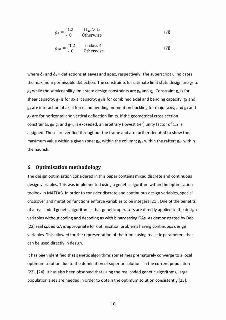
Figure 3 Flowchart of genetic algorithm
Figure 4 Details of eaves haunch cut from universal beam section. The white area in the
figure on the right‐hand side is wastage
START
Generate Initial Population
Frame Analysis
Member ULS Check Member SLS Check
Fitness Evaluation
Fitness Ranking
Elite Preservation
Roulette Selection
Scattered Crossover
Convergence Criteria Satisfied
END
No
Yes
hH

27
Figure 5 Convergence history for different genetic algorithm strategies
(a) Column (b) Rafter
Figure 6 Comparison of optimum cross‐sections for Frame A using UBC3 and FBC2
Fra
me
Wei
gh
t (k
g/m
2 )
28
Figure 7 Optimum frame weight for Lcr = 1.5 m
Fra
me
Wei
ght
(kg/
m2)

29
(a) UBC3
(b) FBC2
Figure 8 Contour of frame weight (kg/m2) for (a) UBC3 and (b) FBC2 with Lcr = 1.5 m

30
Figure 9 Contour of percentage saving in frame weight of FBC2/UBC3 with Lcr = 1.5 m

31
(a)
Figure 10 Contour of percentage increase in frame weight for (a) UBC3 when increasing Lcr
from 1.5 m to 3.5 m, and FBC2 when increasing Lcr from 1.5 m to (b) 2.5m and (c) 3.5 m

32
(b)
Figure 10 Contour of percentage increase in frame weight for (a) UBC3 when increasing Lcr
from 1.5 m to 3.5 m, and FBC2 when increasing Lcr from 1.5 m to (b) 2.5m and (c) 3.5 m

33
(c)
Figure 10 Contour of percentage increase in frame weight for (a) UBC3 when increasing Lcr
from 1.5 m to 3.5 m, and FBC2 when increasing Lcr from 1.5 m to (b) 2.5m and (c) 3.5 m

34
Tables
Table 1 Reliability of genetic algorithm for Frame A using UBC3
Optimisation strategy GA population multiplier
5 10 15 20 25 30
Initial Population (IP)
Search Space Reduction (SSR)
Mean weight (kg per m2)
(Standard deviation)
Normal None 47.82 44.44 43.87 43.31 43.28 43.27
(6.44) (1.84) (1.10) (0.71) (0.49) (0.68)
×6 Larger None 47.76 43.73 43.34 43.21 43.07 43.23
(6.27) (1.20) (0.49) (0.65) (0.63) (0.65)
×12 Larger None 46.05 44.58 44.53 44.27 44.39 44.43
(1.76) (1.09) (0.83) (0.44) (0.63) (0.51)
Normal Yes 45.21 43.53 42.97 43.00 42.89 42.89
(1.91) (0.88) (0.50) (0.52) (0.50) (0.48)
×6 Larger Yes 44.39 43.28 43.12 42.89 42.86 42.85
(1.45) (0.65) (0.49) (0.44) (0.43) (0.45)
×12 Larger Yes 45.00 44.28 44.07 44.06 43.97 43.99
(1.00) (0.82) (0.47) (0.43) (0.27) (0.28)
Table 2 Average number of function evolutions for Frame A using UBC3
Optimisation strategy GA population multiplier
5 10 15 20 25 30
Initial Population (IP)
Search Space Reduction (SSR)
Average number of function evaluations
Normal None 815 1645 2490 3261 3996 4876
×6 Larger None 885 1778 2728 3485 4471 5539
×12 Larger None 984 1975 2985 3961 4939 5869
Normal Yes 783 1592 2379 3129 3954 4747
×6 Larger Yes 884 1755 2647 3513 4376 5266
×12 Larger Yes 1000 1968 2959 3871 4851 5923

35
Table 3 Effect on reliability of different number of genetic algorithm runs
Frame UBC1 UBC2 UBC3 UBC4 FBC1 FBC2 FBC3
(meanweight10runs‐meanweight30runs)/meanweight30runs
A (40 m) 0.02% 0.39% 0.13% ‐0.48% 2.35% 1.25% 1.63%
B (50 m) 0.00% 0.20% 0.00% 0.22% ‐0.38% 1.69% 2.50%
C (60 m) 0.93% 0.39% 4.03%
Table 4 Comparison with previous results in the literature
Benchmark Researchers Column sections Rafter sections Depth of haunch (m) Length of haunch
(m)
Issa and Mohammad (2010) Issa and Mohammad (2010) 457×152×52 406×140×46 0.11 2.45
Phan et al. (2013) 457×152×52 356×127×33 0.49 3.60
UBC3 457×152×52 356×127×33 n/a 5.13
Phan et al. (2013) Phan et al. (2013) 610×229×113 533×210×82 0.515 4.20
UBC3 610×229×113 533×210×82 n/a 4.99

36
Table 5 Optimisation of Frames A & B composed of universal beams
Case Frame Column section Rafter section Haunch section HL (span %)ULS LTB SLS Frame
weight (kg/m2)
g3C g3R g3H Max ofg4C/g5C
Max of g4R/g5R
Max of g6R/g7R
UBC1 A 838×292×176 UB 762×267×173 UB 762×267×173 UB 10.0% 0.80 0.47 0.48 0.85 0.52 0.94 46.75
B 1016×305×272 UB 1016×305×249UB 1016×305×249 UB 10.0% 0.74 0.47 0.45 0.78 0.49 0.97 68.07
UBC2 A 914×305×201 UB 762×267×134 UB 610×305×179 UB 10.0% 0.68 0.74 0.61 0.72 0.58 1.00 42.54
B 1016×305×272 UB 1016×305×249 UB 762×267×197 UB 10.0% 0.74 0.57 0.46 0.78 0.49 0.99 67.10
UBC3 A 914×305×201 UB 686×254×140 UB 686×254×140 UB 14.3% 0.70 0.65 0.51 0.74 0.57 1.00 43.81
B 1016×305×272 UB 1016×305×249 UB 1016×305×249 UB 7.6% 0.72 0.51 0.51 0.77 0.50 1.00 67.12
UBC4 A 914×305×201 UB 762×267×134 UB 610×305×179 UB 14.1% 0.68 0.74 0.61 0.72 0.58 1.00 42.52
B 1016×305×272 UB 1016×305×222 UB 838×292×226 UB 11.5% 0.76 0.58 0.46 0.81 0.51 1.00 65.51
Table 6 Optimisation of Frames A, B & C composed of fabricated beams using Lcr = 1.5 m
Case FrameColumn section dimensions (mm)
Rafter section dimensions (mm)
Haunch section dimensions (mm)
HL (span %)
ULS LTB SLS Frame weight (kg/m2)
g3C g3R g3H Max ofg4C/g5C
Max ofg4R/g5R
Max ofg6R/g7R
FBC1
A 1336×186×177 FB 692×186×114 FB 692×186×114 FB 16.1% 0.82 0.78 0.54 1.00 0.69 1.00 37.59
B 1708×171×273 FB 891×171×170 FB 891×171×170 FB 17.2% 0.77 0.73 0.49 1.00 0.66 1.00 56.09
C 1893×227×365 FB 1110×227×243 FB 1110×227×243 FB 15.3% 0.79 0.65 0.46 0.94 0.57 1.00 72.51
FBC2
A 1262×204×167 FB 784×122×120 FB 784×122×120 FB 12.6% 0.82 0.75 0.63 0.96 0.88 0.98 37.04
B 1352×272×228 FB 1000×89×190 FB 1000×89×190 FB 15.4% 0.89 0.61 0.49 0.94 0.91 0.99 55.47
C 1653×398×316 FB 1241×125×250 FB 1241×125×250 FB 15.8% 0.83 0.61 0.44 0.83 0.82 1.00 70.49
FBC3
A 965×277×143 FB 940×182×136 FB 302×148×103 FB 5.7% 0.94 0.94 0.83 0.98 0.84 0.99 36.06
B 1086×385×202 FB 1425×159×206 FB 231×182×127 FB 7.6% 0.99 0.81 0.69 0.98 0.99 0.98 53.13
C 1530×281×280 FB 1544×239×268 FB 114×509×233 FB 4.3% 0.93 0.94 0.84 0.98 0.68 0.97 66.21

37
Table 7 Optimisation of Frames A, B & C composed of fabricated beams using Lcr = 2.5 m
Case FrameColumn section dimensions (mm)
Rafter section dimensions (mm)
Haunch section dimensions (mm)
HL (span %) ULS LTB SLS Frame
weight (kg/m2)
g3C g3R g3H Max ofg4C/g5C
Max ofg4R/g5R
Max ofg6R/g7R
FBC1
A 1344×232×189 FB 708×232×124 FB 708×232×124 FB 10.7% 0.71 0.74 0.73 0.98 0.75 1.00 39.26
B 1627×251×274 FB 888×251×182 FB 888×251×182 FB 14.1% 0.75 0.68 0.53 1.00 0.68 1.00 57.59
C 1775×324×356 FB 1050×324×248 FB 1050×324×248 FB 16.7% 0.80 0.65 0.43 0.96 0.56 1.00 73.78
FBC2
A 1139×252×174 FB 722×167×117 FB 722×167×117 FB 16.0% 0.80 0.74 0.53 0.97 0.94 0.99 37.91
B 1493×321×256 FB 978×167×194 FB 978×167×194 FB 11.5% 0.75 0.66 0.60 0.87 0.89 0.98 57.49
C 1710×295×324 FB 1126×129×254 FB 1126×129×254 FB 14.7% 0.80 0.64 0.46 0.96 0.98 1.00 71.20
FBC3
A 986×321×156 FB 917×161×133 FB 395×182×128 FB 5.2% 0.84 0.89 0.75 0.94 0.99 0.97 36.93
B 1299×333×213 FB 1253×197×207 FB 290×219×111 FB 4.1% 0.87 0.87 0.81 1.00 0.93 0.95 52.92
C 1395×395×301 FB 1549×213×266 FB 168×355×176 FB 4.8% 0.86 0.92 0.82 0.92 0.92 0.98 67.10
Table 8 Optimal designs with serviceability limits removed
Case FrameColumn section dimensions (mm)
Rafter section dimensions (mm)
Haunch section dimensions (mm)
HL (span %) ULS LTB
Frame weight (kg/m2) g3C g3R g3H
Max ofg4C/g5C
Max ofg4R/g5R
UBC1 A 610×229×113 UB 610×229×113 UB 610×229×113 UB 10% 0.89 0.91 0.86 0.93 0.77 35.47
B 686×254×152 UB 686×254×152 UB 686×254×152 UB 10% 0.95 0.99 0.96 0.99 0.80 46.03
FBC1
A 533×337×110 FB 533×337×110 FB 533×337×110 FB 12.1% 0.89 0.99 0.99 1.00 0.85 34.57
B 671×310×148 FB 671×310×148 FB 671×310×148 FB 10.9% 0.83 0.99 0.99 1.00 0.85 47.01
C 760×374×197 FB 760×374×197 FB 760×374×197 FB 12.3% 0.91 1.00 0.88 1.00 0.76 57.50