Embed Size (px)
DESCRIPTION
Notes on optimal control theory
Citation preview

Section 20.1 fromFundamental methods of Mathematical Economics, McGraw Hill 2005, 4th Edition.By A. C. Chiang & Kevin Wainwright is covered. The nature of optimal controlRead page 631-632 from book. The summary is as follows:
The optimal control problem is
Maximize ∫0
T
F (t , y ,u )dt
Subject to y '=f (t , y , u)y (0 )=A , y (T ) free and u(t) is unrestricted.
t is time, y(t) is known as state variable, u(t) as control variable.
The objective function is an integral ∫0
T
F ( t , y ,u )dt whose integrand F ( t , y , u ) stipulates how the
choice of the control variable u at time t, along with the resulting y at time t, determines our object of maximization at t.
The equation y '=f (t , y , u) is equation of motion for state variable. This equation provides the
mechanism whereby our choice of control variable u can be translated into a specific pattern of movement of the state variable y.
In equationy (0 )=A , y (T ) free, we indicate that initial state, the value of y at t=0, is a constant A,
but the terminal state y (T )is left unrestricted. u(t) is unrestricted its possible for u to be limited to a control region.
Pontryagin’s maximum principalRead page 633-634 from book. The summary is as follows:The HamiltonianThe Hamiltonian is defined as
H ( t , y ,u , λ )=F (t , y , u )+λ ( t ) f (t , y , u)
Where λ (t ) is known as the costate variable, H denotes the Hamiltonian and is a function of four
variables: t, y, u and λ . Like the Lagrange multiplier, the costate variable λ (t ) measures the shadow price of the state variable.
1
The maximum principalThe various components of maximum principal are as follows:
(i)∂ H∂u
=0 and ∂2 H∂u2 <0
(ii) y '=∂ H∂ λ
(state equation)
(iii) λ '=−∂ H∂ y
(costate equation)
(iv) λ (T )=0 (transversality condition)
Condition (i) states that at every time t the value of u(t), the optimal control, must be chosen so as to maximize the value of Hamiltonian over all admissible values of u(t).
Conditions (ii) and (iii) of maximum principal, y '=∂ H∂ λ
and λ'=−∂ H
∂ y give us two equations of
motion, referred to as the Hamiltonian system for the given problem.
Condition (iv), is the transversality condition appropriate for the free-terminal-state problem only.
Example 1: Find the optimal control path that will
Maximize ∫0
1
( y−u2)dt
Subject to y '=uAnd y (0 )=2 , y (1 ) free
Solution:Step I: Write the Hamiltonian and calculate its partial derivatives with respect to y ,u , λ.The Hamiltonian for this problem is
H= y−u2+λu
∂ H∂u
=−2u+ λ ,∂ H∂ λ
=u ,∂ H∂ y
=1 ,∂2 H∂u2 =−2
Step II: Write the various components of maximum principal.The various components of maximum principal are as follows:
(i)∂ H∂u
=−2u+ λ=0∨¿
2
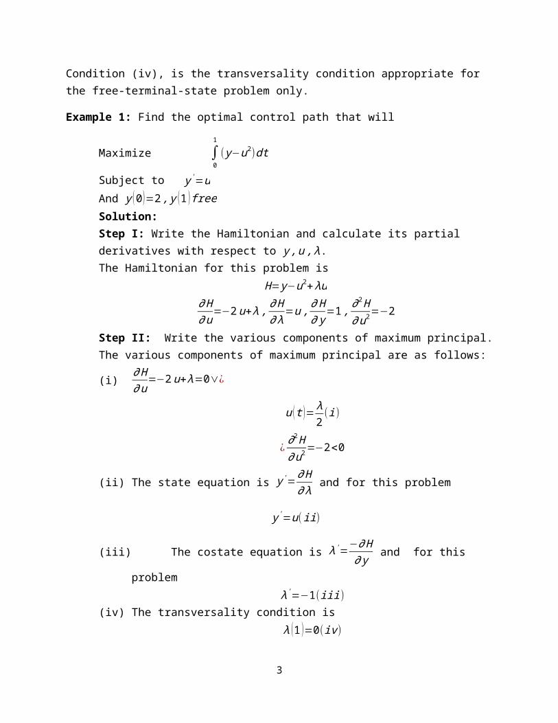
u (t )= λ2(i)
¿ ∂2 H∂u2 =−2<0
(ii) The state equation is y '=∂ H∂ λ
and for this problem
y '=u(ii)
(iii) The costate equation is λ'=−∂ H
∂ y and for this problem
λ '=−1(iii)(iv) The transversality condition is
λ (1 )=0(iv)Equations (ii) and (iii) constitute differential equation system for this problem.
Step III: We want to find u¿), y (t ) and λ (t) from equations (i) to (iii) satisfying the
transversality condition (iv) and initial condition y (0 )=2.
We can first solve for λ by straight integration of (iii) to get
λ (t )=c1−t (c1 arbitrary )(v )
Using the transversality condition λ (1 )=0in (vi), we have0=c1−1∨c1=1
Thus the optimal costate path is λ (t )=1−t(vi)Using λ (t) from (vi) in (i), the corresponding optimal control path is
u (t )=12
(1−t )(vii)
Using (vii) in (ii), we have
y '=1−t2
and by integration, we have
y (t )= t2− t 2
4+c2(c2 arbitrary)
The arbitrary constant canbe definitizeby using theinitial condition y (0 )=2.
Setting t=0 in the preceding equation, we get c2=2. Thus the optimal path for state variable is
y (t )= t2− t 2
4+2.
3

The optimal control path is
u (t )=12
(1−t )∧optimal path for statevariable is y ( t )= t2−t 2
4+2 with costate variable
λ (t )=1−t .
Example 2: Find the optimal control path that will
Maximize ∫0
T
−( 1+u2 )12 dt
Subject to y '=uAnd y (0 )=A , y (T ) free
Solution:Step I: Write the Hamiltonian and calculate its partial derivatives with respect to y ,u , λ.The Hamiltonian for this problem is
H=− (1+u2 )12+ λu
∂ H∂u
= −u
(1+u2)12
+λ ,∂ H∂ λ
=u ,∂ H∂ y
=0 ,∂2 H
∂ u2=−(1+u2 )
−32
Step II: Write the various components of maximum principal.The various components of maximum principal are as follows:
(i)∂ H∂u
= −u
(1+u2)12
+λ=0(i)
¿ ∂2 H
∂u2=−( 1+u2 )
−32 <0
(ii) The state equation is y '=∂ H∂ λ
and for this problem
y '=u(ii)
(iii) The costate equation is λ'=−∂ H
∂ y and for this problem
λ '=0(iii)(iv) The transversality condition is
λ (T )=0 (iv)Equations (ii) and (iii) constitute differential equation system for this problem.
Step III: We want to find u¿), y (t ) and λ (t) from equations (i) to (iii) satisfying the
transversality condition (iv) and initial condition y (0 )=A.
We can first solve for λ by straight integration of (iii) to get
4

λ (t )=c1 (c1 arbitrary )(v )
Using the transversality condition λ (T )=0in (vi), we have0=c1
Thus the optimal costate path is λ (t )=0 (vi)Using λ (t) from (vi) in (i), the corresponding optimal control path is
u (t )=0(vii)
Using (vii) in (ii), we have
y '=0and by integration, we have
y (t )=c2(c2 arbitrary)The arbitrary constant canbe definitizeby using theinitial condition y (0 )=A.
Setting t=0 in the preceding equation, we get c2=A. Thus the optimal path for state variable is
y (t )=A .
The optimal control path is u (t )=0 , optimal path for state variable is y (t )=A with costate
variable λ (t )=0.
Example 3: Find the optimal control path that will
Maximize ∫0
1
( y−u2)dt
Subject to y '=uAnd y (0 )=5 , y (1 ) free
Step I: Write the Hamiltonian and calculate its partial derivatives with respect to y ,u , λ.The Hamiltonian for this problem is
H= y−u2+λu
∂ H∂u
=−2u+ λ ,∂ H∂ λ
=u ,∂ H∂ y
=1 ,∂2 H∂u2 =−2
Step II: Write the various components of maximum principal.The various components of maximum principal are as follows:
(i)∂ H∂u
=−2u+ λ=0∨¿
u (t )= λ2(i)
¿ ∂2 H∂u2 =−2<0
5

(ii) The state equation is y '=∂ H∂ λ
and for this problem
y '=u(ii)
(iii) The costate equation is λ'=−∂ H
∂ y and for this problem
λ '=−1(iii)(iv) The transversality condition is
λ (1 )=0(iv)Equations (ii) and (iii) constitute differential equation system for this problem.
Step III: We want to findu¿), y (t ) and λ (t) from equations (i) to (iii) satisfying the
transversality condition (iv) and initial condition y (0 )=5.
We can first solve for λ by straight integration of (iii) to get
λ (t )=c1−t (c1 arbitrary )(v )
Using the transversality condition λ (1 )=0in (vi), we have0=c1−1∨c1=1
Thus the optimal costate path is λ (t )=1−t(vi)Using λ (t) from (vi) in (i), the corresponding optimal control path is
u (t )=12
(1−t )(vii)
Using (vii) in (ii), we have
y '=1−t2
and by integration, we have
y (t )= t2− t 2
4+c2(c2 arbitrary)
The arbitrary constant canbe definitizeby using theinitial condition y (0 )=5.
Setting t=0 in the preceding equation, we get c2=5. Thus the optimal path for state variable is
y (t )= t2− t 2
4+5.
The optimal control path is
u (t )=12
(1−t )∧optimal path for statevariable is y ( t )= t2−t 2
4+5 with costate variable
λ (t )=1−t .
6

Example 4: Find the optimal control path that will
Maximize ∫0
2
( 2 y−3u−au2 ) dt , a>0
Subject to y '=u+ yAnd y (0 )=5 , y (2 ) free
Step I: Write the Hamiltonian and calculate its partial derivatives with respect to y ,u , λ.The Hamiltonian for this problem is
H=2 y−3u−a u2+λ (u+ y )∂ H∂u
=−3−2 au+ λ ,∂ H∂ λ
=u+ y ,∂ H∂ y
=2+ λ ,∂2 H∂ u2 =−2 a
Step II: Write the various components of maximum principal.The various components of maximum principal are as follows:
(i)∂ H∂u
=−3−2 au+ λ=0∨¿
u (t )= 12a
( λ−3)(i)
¿ ∂2 H∂u2 =−2a<0 as a>0
(ii) The state equation is y '=∂ H∂ λ
and for this problem
y '=u+ y ( ii)
(iii) The costate equation is λ'=−∂ H
∂ y and for this problem
λ '=−2−λ (iii)(iv) The transversality condition is
λ (2 )=0(iv)Equations (ii) and (iii) constitute differential equation system for this problem.
Step III: We want to find u¿), y (t ) and λ (t) from equations (i) to (iii) satisfying the
transversality condition (iv) and initial condition y (0 )=5.
We can write equation (iii) as
λ '+λ=−2(v )
This linear first order ordinary differential equation for λ and its integrating factor is
e∫dt=e t
Multiplying (v) by e t, we have
λ ' e t+λ et=−2e t
7

this yields ddt
[ λ e t ]=−2e t
Integrating both sides, we have
∫ ddt
[ λ e t ]dt=∫−2 e t dt⇒ λ e t=−2 e t+c1
λ (t )=c1 e−t−2 ( c1 arbitrary )(vi)Using the transversality condition λ (2 )=0in (vi), we have
0=c1e−2−2∨c1=2e2
Thus the optimal costate path is λ (t )=2(e2−t−1)(vii)Using λ (t) from (vii) in (i), the corresponding optimal control path is
u (t )= 12a
(2 e2−t−5 ) (viii)
Using (viii) in (ii), we have
y '− y= 12 a
(2 e2−t−5 )(ix)
Solving (ix) by integrating factor method, we have
y (t )= 52 a
− e2−t
2a+c2 et (c2arbitrary )
The arbitrary constant canbe definitizeby using theinitial condition y (0 )=5.
Setting t=0 in the preceding equation, we get c2=e2
2 a-
52 a
+5. Thus the optimal path for
state variable is
y (t )= 52 a
− e2−t
2a+¿
The optimal control path is u (t )= 12a
(2 e2−t−5 )∧optimal path for state variable is
y (t )= 52 a
− e2−t
2a+¿with costate variable λ (t )=2 (e2−t−1 )
Example 5: Find the optimal control path that will
Maximize ∫0
T
(−au+b u2)dt
Subject to y '= y−uAnd y (0 )= yo , y (T ) free
8

Solution:Step I: Write the Hamiltonian and calculate its partial derivatives with respect to y ,u , λ.The Hamiltonian for this problem is
H=−au+b u2+λ ( y−u)∂ H∂u
=−a+2 bu−λ ,∂ H∂ λ
= y−u ,∂ H∂ y
=λ ,∂2 H∂u2 =2 b
Step II: Write the various components of maximum principal.The various components of maximum principal are as follows:
(i)∂ H∂u
=−a+2 bu−λ=0∨¿
u (t )= 12b
( λ+a)(i)
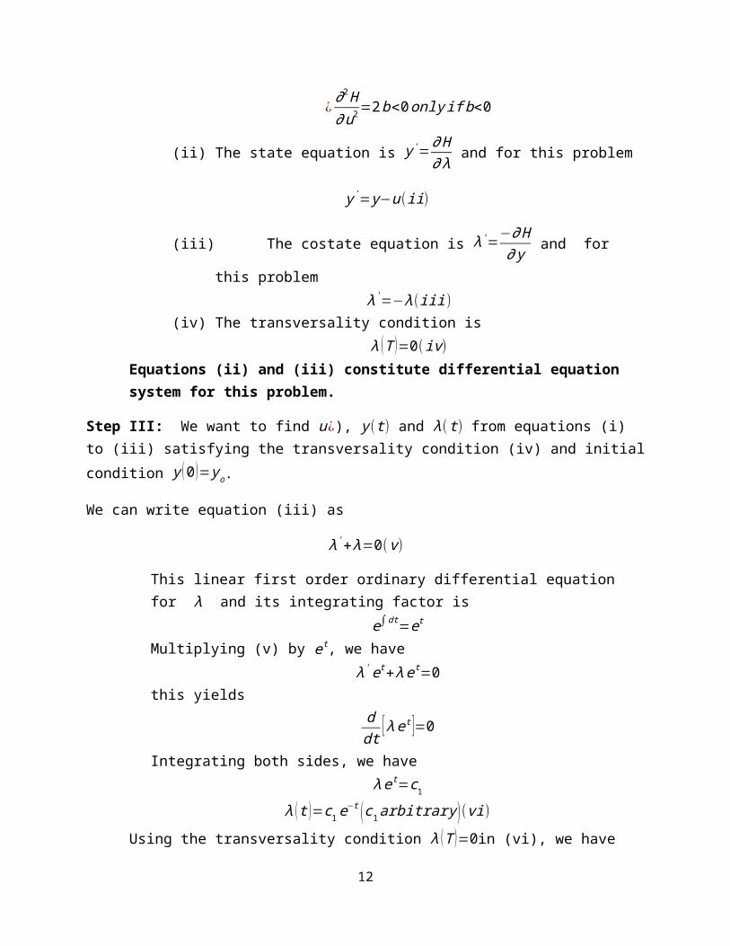
¿ ∂2 H∂u2 =2 b<0 only if b<0
(ii) The state equation is y '=∂ H∂ λ
and for this problem
y '= y−u(ii)
(iii) The costate equation is λ'=−∂ H
∂ y and for this problem
λ '=−λ(iii )(iv) The transversality condition is
λ (T )=0 (iv)Equations (ii) and (iii) constitute differential equation system for this problem.
Step III: We want to find u¿), y (t ) and λ (t) from equations (i) to (iii) satisfying the
transversality condition (iv) and initial condition y (0 )= yo.
We can write equation (iii) as
λ '+λ=0 (v )
This linear first order ordinary differential equation for λ and its integrating factor is
e∫dt=e t
Multiplying (v) by e t, we have
λ ' e t+λ et=0this yields
ddt
[ λ e t ]=0
Integrating both sides, we have
λ e t=c1
9

λ (t )=c1 e−t (c1 arbitrary )(vi)Using the transversality condition λ (T )=0in (vi), we have
0=c1e−T∨c1=0
Thus the optimal costate path is λ (t )=0 (vi)Using λ (t) from (vi) in (i), the corresponding optimal control path is
u (t )= a2b
(vii)
Using (vii) in (ii), we have
y '= y− a2 b
y '− y=−a2 b
(viii)
The integrating factor for (viii) is
e∫−dt=e−t
Multiplying (viii) by e−t, we have
y ' e−t− y e−t=−a2b
e−t
this yields ddt
[ y e−t ]=−a2 b
e−t
Integrating both sides, we have
∫ ddt
[ y e−t ] dt=∫−a2 b
e−t dt⇒ y e−t= a2 b
e−t+c2
y (t )= a2 b
+c2 et ( c2arbitrary )(ix)
The arbitrary constant canbe definitizeby using theinitial condition y (0 )= yo.
Setting t=0 in the preceding equation, we get c2= y o−a
2b. Thus the optimal path for state
variable is
y (t )= a2 b
+( yo−a
2 b)e t
.
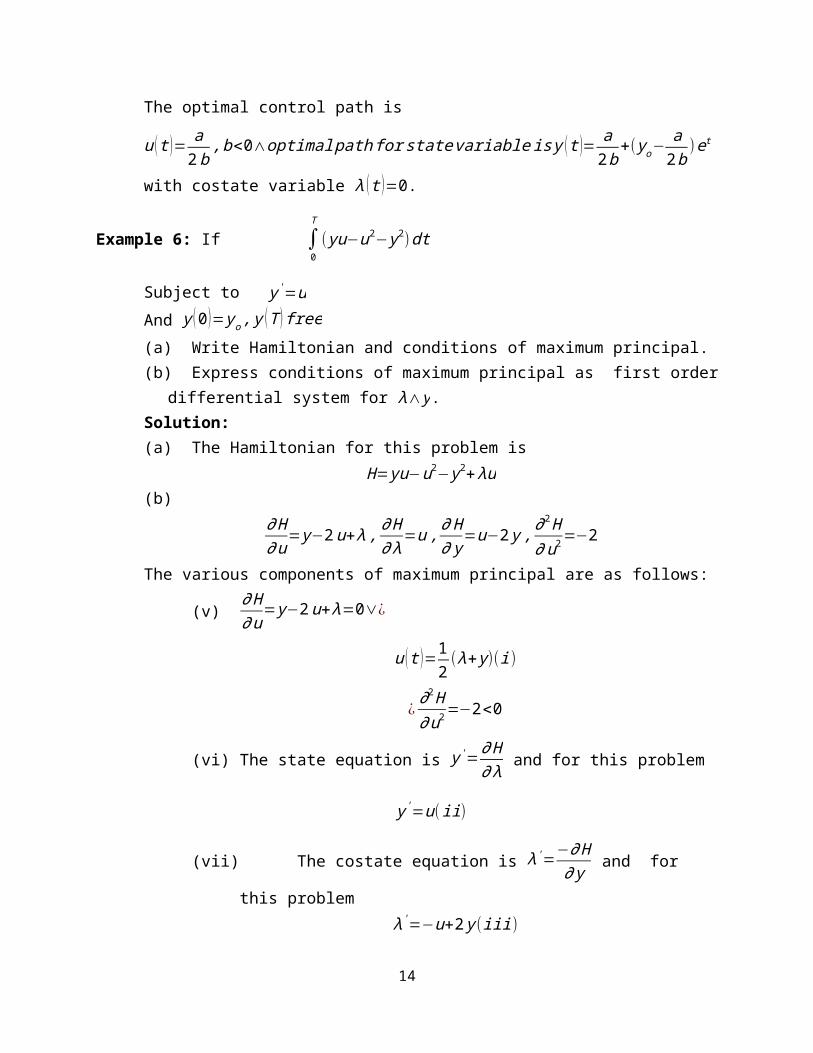
The optimal control path is
u (t )= a2b
,b<0∧optimal path for statevariable is y ( t )= a2 b
+( yo−a
2 b)e t
with costate
variable λ (t )=0.
10

Example 6: If ∫0
T
( yu−u2− y2)dt
Subject to y '=uAnd y (0 )= yo , y (T ) free
(a) Write Hamiltonian and conditions of maximum principal.(b) Express conditions of maximum principal as first order differential system for λ∧ y.Solution:(a) The Hamiltonian for this problem is
H= yu−u2− y2+ λu(b)
∂ H∂u
= y−2 u+λ ,∂ H∂ λ
=u ,∂ H∂ y
=u−2 y ,∂2 H∂ u2 =−2
The various components of maximum principal are as follows:
(v)∂ H∂u
= y−2 u+λ=0∨¿
u (t )=12(λ+ y )(i)
¿ ∂2 H∂u2 =−2<0
(vi) The state equation is y '=∂ H∂ λ
and for this problem
y '=u(ii)
(vii) The costate equation is λ'=−∂ H
∂ y and for this problem
λ '=−u+2 y (iii)(viii) The transversality condition is
λ (T )=0 (iv)(c) Using (i) in (ii) and (iii), we have
y '=12
( λ+ y )
¿
y '− y2= λ
2(v )
And
11
λ '=−12
( λ+ y )+2 y
Or
λ '+ λ2=3 y
2( vi )
Equation (v) and (vi) form first order differential system for λ∧ y . We can solve it for λ∧ y
subject to transversality condition λ (T )=0and initial condition y (0 )= yo .
Section 20.2 fromFundamental methods of Mathematical Economics, McGraw Hill 2005, 4th Edition.By A. C. Chiang & Kevin Wainwright is covered. Fixed terminal pointThe optimal control problem is
Maximize ∫0
T
F ( t , y ,u )dt
Subject to y '=f (t , y , u)y (0 )=A , y (T )= yT and u(t) is unrestricted.
Both T ,∧ yT are given. u(t) is unrestricted its possible for u to be limited to a control region.
The Hamiltonian is defined as
H ( t , y ,u , λ )=F (t , y , u )+λ ( t ) f (t , y , u)The various components of maximum principal are as follows:
(v)∂ H∂u
=0 and ∂2 H∂u2 <0
(vi) y '=∂ H∂ λ
(state equation)
(vii) λ '=−∂ H∂ y
(costate equation)
In this case, no transversality condition is needed as the terminal condition itself should provide information to definitize one constant.
Example 1: Find the optimal control path that will
Maximize ∫0
1
( y−u2)dt
Subject to y '=u
12

And y (0 )=2 , y (1 )=a
Solution:Step I: Write the Hamiltonian and calculate its partial derivatives with respect to y ,u , λ.The Hamiltonian for this problem is
H= y−u2+λu
∂ H∂u
=−2u+ λ ,∂ H∂ λ
=u ,∂ H∂ y
=1 ,∂2 H∂u2 =−2
Step II: Write the various components of maximum principal.The various components of maximum principal are as follows:
(v)∂ H∂u
=−2u+ λ=0∨¿
u (t )= λ2(i)
¿ ∂2 H∂u2 =−2<0
(vi) The state equation is y '=∂ H∂ λ
and for this problem
y '=u(ii)
(vii) The costate equation is λ'=−∂ H
∂ y and for this problem
λ '=−1(iii)Equations (ii) and (iii) constitute differential equation system for this problem.
Step III: We want to find u¿), y (t ) and λ (t) from equations (i) to (iii) satisfying the initial
condition y (0 )=2 and terminal condition y (1 )=a .
Combining (i) and (ii), we have
y '= λ2(iv)
We can first solve for λ by straight integration of (iii) to get
λ (t )=c1−t (c1 arbitrary )(v )
Using (v) in (iv), we have
y '=12
(c1−t )
and by integration, we have
13
y (t )= t2
c1−t 2
4+c2 (c2 arbitrary ) (vi)
The arbitrary constantscanbe definitize byusing the initialcondition y (0 )=2 and and
terminal condition y (1 )=a .
Using y (0 )=2 in (vi), we have2=c2
Using y (1 )=a in (vi), we have
a=12
c1−14+c2
a=12
c1−14+2(asc2=2)
Or c1=2 a−72
Thus the optimal path for state variable is
y (t )=(a−74 ) t−t 2
4+2 (vii)
The optimal path for costate variable and control variable is
λ (t )=2 a−72−t(by ( v ))
And
u (t )=a−74− t
2(by (i ))
Example 2: Find the optimal control path that will
Maximize ∫1
2
( y+ut−u2 ) dt
Subject to y '=uAnd y (1 )=3 , y (2 )=4
Solution:
Step I: Write the Hamiltonian and calculate its partial derivatives with respect to y ,u , λ.The Hamiltonian for this problem is
H= y+ut−u2+ λu
∂ H∂u
=t−2u+ λ ,∂ H∂ λ
=u ,∂ H∂ y
=1 ,∂2 H∂ u2 =−2
Step II: Write the various components of maximum principal.The various components of maximum principal are as follows:
(i)∂ H∂u
=t−2u+ λ=0∨¿
14

u (t )= λ+t2
(i)
¿ ∂2 H∂u2 =−2<0
(ii) The state equation is y '=∂ H∂ λ
and for this problem
y '=u(ii)
(iii) The costate equation is λ'=−∂ H
∂ y and for this problem
λ '=−1(iii)
Step III: We want to find u¿), y (t ) and λ (t) from equations (i) to (iii) satisfying the initial
condition y (1 )=3 and terminal condition y (2 )=4.
Combining (i) and (ii), We have
y '= λ+t2
(iv)
We can first solve for λ by straight integration of (iii) to get
λ (t )=c1−t (c1 arbitrary )(v )
Substituting λ from (v) in (iv), we have
y '=c1
2(vi)
And by straight integration, we have
y=c1
2t +c2(vii)
The arbitrary constantscanbe definitize byusing the initialconditiony (1 )=3∧terminalcondition y (2 )=4.
Using y (1 )=3 in (vii), we have
3=c1
2+c2(viii)
Using y (2 )=4 in (vii), we have4=c1+c2(ix)
Solving (viii) and (ix) for c1 and c2 , we havec1=2 , c2=2
Thus the optimal path for state variable isy (t )=t+2
15

The optimal path for costate variable and control variable is
λ (t )=2−t(by ( v ))
andu (t )=1(by ( i ))
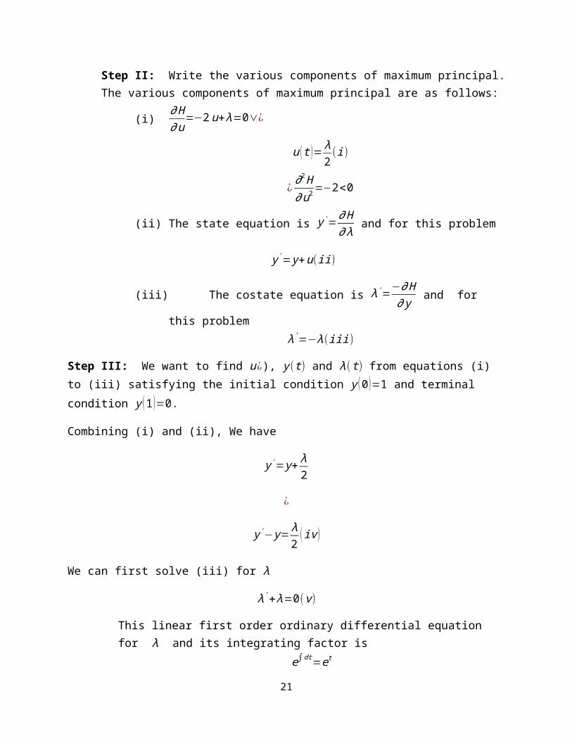
Example 3: Find the optimal control path that will
Maximize ∫0
1
−u2dt
Subject to y '= y+uAnd y (0 )=1 , y (1 )=0
Solution:
Step I: Write the Hamiltonian and calculate its partial derivatives with respect to y ,u , λ.The Hamiltonian for this problem is
H=−u2+ λ( y+u)∂ H∂u
=−2u+ λ ,∂ H∂ λ
= y+u ,∂ H∂ y
= λ ,∂2 H∂ u2 =−2
Step II: Write the various components of maximum principal.The various components of maximum principal are as follows:
(i)∂ H∂u
=−2u+ λ=0∨¿
u (t )= λ2(i)
¿ ∂2 H∂u2 =−2<0
(ii) The state equation is y '=∂ H∂ λ
and for this problem
y '= y+u( ii)
(iii) The costate equation is λ'=−∂ H
∂ y and for this problem
λ '=−λ(iii )
Step III: We want to find u¿), y (t ) and λ (t) from equations (i) to (iii) satisfying the initial
condition y (0 )=1 and terminal condition y (1 )=0.
Combining (i) and (ii), We have
16
y '= y+ λ2
¿
y '− y= λ2
( iv )
We can first solve (iii) for λ
λ '+λ=0 (v )
This linear first order ordinary differential equation for λ and its integrating factor is
e∫dt=e t
Multiplying (v) by e t, we have
λ ' e t+λ et=0this yields
ddt
[ λ e t ]=0
Integrating both sides, we have
λ e t=c1
λ (t )=c1 e−t (c1 arbitrary )(vi)
Substituting λ from (vi) in (iv), we have
y '− y=c1 e−t
2(vii)
The integrating factor for (vii) is
e∫−dt=e−t
Multiplying (vii) by e−t, we have
y ' e−t− y e−t=c1 e−2 t
2this yields
ddt
[ y e−t ]= c1 e−2 t
2Integrating both sides, we have
∫ ddt
[ y e−t ] dt=∫ c1e−2 t
2dt⇒ y e−t=
−c1 e−2 t
4+c2
y (t )=−c1 e−t
4+c2 et ( c2 arbitrary )(viii)
17

The arbitrary constantscanbe definitize byusing the initialconditiony (0 )=1∧terminalcondition y (1 )=0.
Using y (0 )=1 in (viii), we have
1=−c1
4+c2(ix)
Using y (1 )=0 in (viii), we have
0=−c1 e−1
4+c2 e (x)
Solving (ix) and (x) for c1 and c2 , we have
c1=4e2
1−e2 , c2=1
1−e2
Thus the optimal path for state variable is
y (t )= 1
1−e2[e t−e2−t]
The optimal path for costate variable and control variable is
λ (t )= 4e2
1−e2 e−t (by (vi ))
and
u (t )= 2 e2
1−e2 e−t(by (i ))
Section 20.3Fundamental methods of Mathematical Economics, McGraw Hill 2005, 4th Edition.By A. C. Chiang & Kevin Wainwright is covered.
18

The optimal control problem is
Maximize ∫0
T
F ( y , u ) e−rt dt
Subject to y '=f ( y , u)and conditions
19

t is time, y(t) is known as state variable, u(t) as control variable.
Hamiltonian function and Pontryagin’s maximum principalThe Hamiltonian is defined as
H (t , y ,u , λ )=F ( y , u ) e−rt+λ (t ) f ( y ,u )(1)
Where λ (t ) is known as the costate variable, H denotes the Hamiltonian and is a function of four
variables: t, y, u and λ . Like the Lagrange multiplier, the costate variable λ (t ) measures the shadow price of the state variable.
The various components of maximum principal are as follows:
(viii)∂ H∂u
=0 and ∂2 H∂u2 <0
(ix) y '=∂ H∂ λ
(state equation)
(x) λ '=−∂ H∂ y
(costate equation)
Current value Hamiltonian and maximum principalThe current value Hamiltonian is defined as
H c ( y ,u , λ )=F ( y ,u )+μ ( t ) f ( y , u)
Where μ (t ) is known as the costate variable, H denotes the Hamiltonian and is a function of four
variables: t, y, u and λ . Like the Lagrange multiplier, the costate variable μ ( t ) measures the shadow price of the state variable.
The various components of maximum principal are as follows:
(i)∂ H c
∂ u=0 and
∂2 H c
∂ u2 <0
(ii) y '=∂ H c
∂ μ (state equation)
(iii) μ'=−∂ H c
∂ y+rμ (costate equation)
1. Find the optimal control path that will
Maximize ∫0
T
( 2 y−3u−u2 ) e−rt dt
Subject to y '= y+u(d) Write present value Hamiltonian and conditions of maximum principal.(e) Write current value Hamiltonian and conditions of maximum principal.
20
2. Find the optimal control path that will
Maximize ∫0
T
(−2 u−u2)e−rt dt
Subject to y '= y−u(a) Write current value Hamiltonian and conditions of maximum principal (b) Express conditions of maximum principal as first order differential system for
μ∧ y.(c) Solve the differential system obtained in part (b) for μ(t )∧ y (t). Also find the
control variableu(t ).3. Find the optimal control path that will
Maximize ∫0
1
ln (u)e−rt dt
Subject to y '= y−u(a) Write current value Hamiltonian and conditions of maximum principal.(b) Express conditions of maximum principal as first order differential system for
μ∧ y.(f) Solve the differential system obtained in part (b) for μ(t )∧ y (t). Also find the control
variableu(t ).4. Find the optimal control path that will
Maximize ∫0
T
( y−u2)e−rt dt
Subject to y '=u(a) Write current value Hamiltonian and conditions of maximum principal(b) Express conditions of maximum principal as first order differential system for
μ∧ y.(c) Solve the differential system obtained in part (b) for μ(t )∧ y (t). Also find the
control variableu(t ).
21


![Optimal Control and Optimization Methods for Multi-Robot Systems · Optimal control & dynamic programming ! Optimal control [discrete, infinite horizon] ! Dynamic programming solves](https://img.dokumen.tips/doc/110x75/5f73944fbcf5a833b2704885/optimal-control-and-optimization-methods-for-multi-robot-optimal-control-dynamic.jpg)