Embed Size (px)
Citation preview

CHAPTER 3
OPTIMAL CONTROL
“What is now proved was once only imagined.”—William Blake.
3.1 INTRODUCTION
After more than three hundred years of evolution, optimal control theory has been formu-lated as an extension of the calculus of variations. Based on the theoretical foundationlaid by several generations of mathematicians, optimal control has developed into a well-established research area and finds its applications in many scientific fields, ranging frommathematics and engineering to biomedical and management sciences. The maximumprinciple, developed in the late 1950s by Pontryagin and his coworkers [41], is amongthe biggest successes in optimal control. This principle as well as other results in optimalcontrol apply to any problems of the calculus of variations discussed earlier in Chapter 2(and gives equivalent results, as one would expect). This extension is most easily seen byconsidering the prototypical problem of the calculus of variations that consists of choosinga continuously differentiable function x(t), t1 ≤ t ≤ t2, to
minimize:∫ t2
t1
`(t,x(t), x(t)) dt
subject to: x(t1) = x1.
Nonlinear and Dynamic Optimization: From Theory to Practice. By B. Chachuat2007 Automatic Control Laboratory, EPFL, Switzerland
105

106 OPTIMAL CONTROL
Indeed, the above problem is readily transformed into the equivalent problem of finding acontinuously differentiable function u(t), t1 ≤ t ≤ t2, to
minimize:∫ t2
t1
`(t,x(t),u(t)) dt
subject to: x(t) = u(t); x(t1) = x1.
Optimal control refers to this latter class of problems. In optimal control problems, vari-ables are separated into two classes, namely the state (or phase) variables and the controlvariables. The evolution of the former is dictated by the latter, via a set of differentialequations. Further, the control as well as the state variables are generally subject to con-straints, which make many problems in optimal control non-classical, since problems withpath constraints can hardly be handled in the classical calculus of variations. That is, theproblem of optimal control can then be stated as: “Determine the control signals that willcause a system to satisfy the physical constraints and, at the same time, minimize (or maxi-mize) some performance criterion.” A precise mathematical formulation of optimal controlproblems shall be given in 3.2 below.
Despite its successes, however, optimal control theory is by no means complete, es-pecially when it comes to the question of whether an optimal control exists for a givenproblems. The existence problem is of crucial importance, since it does not make muchsense to seek a solution if none exists. As just an example, consider the problem of steeringa system, from a prescribed initial state, to a fixed target, e.g., in minimum time. To find outwhether an optimal control exists, one may start by investigating whether a feasible controlcan be found, i.e., one that satisfies the physical constraints. This latter question is closelyrelated to system controllability in classical control theory, i.e., the ability to transfer thesystem from any initial state to any desired final state in a finite time. Should the systembe uncontrollable, it is then likely that no successful control may be found for some initialstates. And even though the system can be shown to be controllable, there may not exist anoptimal control in the prescribed class of controls. The difficult problem of the existenceof an optimal control shall be further discussed in 3.3.
Another important topic is to actually find an optimal control for a given problem, i.e.,give a ‘recipe’ for operating the system in such a way that it satisfies the constraints in anoptimal manner. Similar to the previous chapters on NLP and on the calculus of variations,our goal shall be to derive algebraic conditions that are either necessary or sufficient foroptimality. These conditions are instrumental for singling out a small class of candidatesfor an optimal control. First, we shall investigate the application of variational methodsto obtain necessary conditions of optimality for problems without state or control pathconstraints in 3.4; this will develop familiarity with the new notation and tools. Then,we shall consider methods based on so-called maximum principles, such as Pontryaginmaximum principle, to address optimal control problems having path constraints in 3.5.
Finally, as most real-world problems are too complex to allow for an analytical solution,computational algorithms are inevitable in solving optimal control problems. As a result,several successful families of algorithms have been developed over the years. We shallpresent both direct and indirect approaches to solving optimal control problems in 3.6.
3.2 PROBLEM STATEMENT
The formulation of an optimal control problem requires several steps: the class of admissiblecontrols is discussed in 3.2.1; the mathematical description (or model) of the system to be

PROBLEM STATEMENT 107
controlled is considered in 3.2.2; the specification of a performance criterion is addressedin 3.2.3; then, the statement of physical constraints that should be satisfied is described in
3.2.4. Optimal criteria are discussed next in 3.2.5. Finally, we close the section with adiscussion on open-loop and closed-loop optimal control laws in 3.2.6.
3.2.1 Admissible Controls
We shall consider the behavior of a system whose state at any instant of time is characterizedbynx ≥ 1 real numbersx1, . . . , xnx (for example, these may be coordinates and velocities).The vector space of the system under consideration is called the phase space. It is assumedthat the system can be controlled, i.e., the system is equipped with controllers whoseposition dictates its future evolution. These controllers are characterized by points u =(u1, . . . , unu) ∈ IRnu , nu ≥ 1, namely the control variables.
In the vast majority of optimal control problems, the values that can be assumed by thecontrol variables are restricted to a certain control regionU , which may be any set in IRnu .In applications, the case where U is a closed region in IRnu is important. For example, thecontrol region U may be a hypercube,
|uj | ≤ 1, j = 1, . . . , nu.
The physical meaning of choosing a closed and bounded control region is clear. The quantityof fuel being supplied to a motor, temperature, current, voltage, etc., which cannot take onarbitrarily large values, may serve as control variables. More general relations, such as
φ(u) = 0,
may also exist among the control variables.We shall call every function u(·), defined on some time interval t0 ≤ t ≤ tf, a control. A
control is an element of a (normed) linear space of real-vector-valued functions. Throughoutthis chapter, we shall consider the class of continuous controls or, more generally, piecewisecontinuous controls (see Fig. 3.1.):
Definition 3.1 (Piecewise Continuous Functions). A real-valued function u(t), t0 ≤ t ≤tf, is said to be piecewise continuous, denoted u ∈ C [t0, tf], if there is a finite (irreducible)partition t0 = θ0 < θ1 < · · · < θN < θN+1 = tf such that u may be regarded as afunction in C [θk, θk+1] for each k = 0, 1, . . . , N .
That is, the class C [t0, tf]nu of nu-dimensional vector-valued analogue of C [t0, tf], con-sists of those controls u with componentsuj ∈ C [t0, tf], j = 1, . . . , nu. The discontinuitiesof one such control are by definition those of any of its components uj .
Note that piecewise continuous controls correspond to the assumption of inertia-lesscontrollers, since the values of u(t) may jump instantaneously when a discontinuity is met.This class of controls appears to be the most interesting for the practical applications of thetheory, although existence of an optimal control is not guaranteed in general, as shall beseen later in 3.3.
The specification of the control region together with a class of controls leads naturallyto the definition of an admissible control:
Definition 3.2 (Admissible Control). A piecewise continuous control u(·), defined onsome time interval t0 ≤ t ≤ tf, with range in the control region U ,
u(t) ∈ U, ∀t ∈ [t0, tf],
108 OPTIMAL CONTROL
is said to be an admissible control.
We shall denote by U[t0, tf] the class of admissible controls on [t0, tf]. It follows fromDefinition 3.1 that every admissible control u ∈ U[t0, tf] is bounded.
PSfrag replacements
t
x(t), u(t)
t0 θ1 θk θN tf
x(·)
u(·)
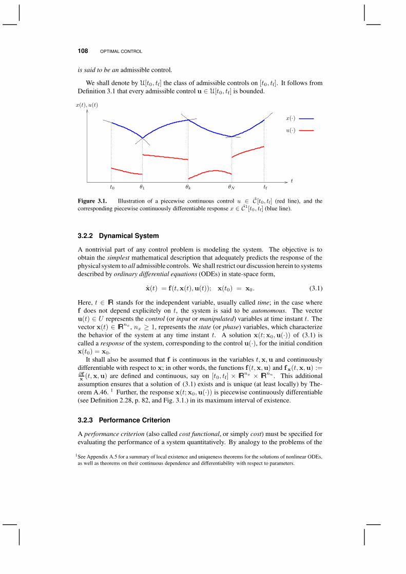
Figure 3.1. Illustration of a piecewise continuous control u ∈ C [t0, tf] (red line), and thecorresponding piecewise continuously differentiable response x ∈ C1[t0, tf] (blue line).
3.2.2 Dynamical System
A nontrivial part of any control problem is modeling the system. The objective is toobtain the simplest mathematical description that adequately predicts the response of thephysical system to all admissible controls. We shall restrict our discussion herein to systemsdescribed by ordinary differential equations (ODEs) in state-space form,
x(t) = f(t,x(t),u(t)); x(t0) = x0. (3.1)
Here, t ∈ IR stands for the independent variable, usually called time; in the case wheref does not depend explicitely on t, the system is said to be autonomous. The vectoru(t) ∈ U represents the control (or input or manipulated) variables at time instant t. Thevector x(t) ∈ IRnx , nx ≥ 1, represents the state (or phase) variables, which characterizethe behavior of the system at any time instant t. A solution x(t;x0,u(·)) of (3.1) iscalled a response of the system, corresponding to the control u(·), for the initial conditionx(t0) = x0.
It shall also be assumed that f is continuous in the variables t,x,u and continuouslydifferentiable with respect to x; in other words, the functions f(t,x,u) and fx(t,x,u) :=∂fx
(t,x,u) are defined and continuous, say on [t0, tf] × IRnx × IRnu . This additionalassumption ensures that a solution of (3.1) exists and is unique (at least locally) by The-orem A.46. 1 Further, the response x(t;x0,u(·)) is piecewise continuously differentiable(see Definition 2.28, p. 82, and Fig. 3.1.) in its maximum interval of existence.
3.2.3 Performance Criterion
A performance criterion (also called cost functional, or simply cost) must be specified forevaluating the performance of a system quantitatively. By analogy to the problems of the
1See Appendix A.5 for a summary of local existence and uniqueness theorems for the solutions of nonlinear ODEs,as well as theorems on their continuous dependence and differentiability with respect to parameters.

PROBLEM STATEMENT 109
calculus of variations (see 2.2.1, p. 63), the cost functional J : U[t0, tf] → IR may bedefined in the so-called Lagrange form,
J(u) :=
∫ tf
t0
`(t,x(t),u(t)) dt. (3.2)
In this chapter, we shall assume that the Lagrangian `(t,x,u) is defined and continuous,together with its partial derivatives `x(t,x,u) on IR × IRnx × IRnu . Moreover, either theinitial time t0 and final time tf may be considered a fixed or a free variable in the optimizationproblem.
The objective functional may as well be specified in the Mayer form,
J(u) :=ϕ(t0,x(t0), tf,x(tf)), (3.3)
with ϕ : IR × IRnx × IR × IRnx → IR being a real-valued function. Again, it shall beassumed throughout that ϕ(t0,x0, tf,xf) and ϕx(t0,x0, tf,xf) exist and are continuous onIR × IRnx × IR × IRnx .
More generally, we may consider the cost functional in the Bolza form, which correspondsto the sum of an integral term and a terminal term as
J(u) :=ϕ(t0,x(t0), tf,x(tf)) +
∫ tf
t0
`(t,x(t),u(t)) dt. (3.4)
Interestingly enough, Mayer, Lagrange and Bolza problem formulations can be shownto be theoretically equivalent:
Lagrange problems can be reduced to Mayer problems by introducing an additionalstate x`, the new state vector x := (x`, x1, . . . , xnx)
T, and an additional differentialequation
x`(t) = `(t,x(t),u(t)); x`(t0) = 0.
Then, the cost functional (3.2) is transformed into one of the Mayer form (3.3) withϕ(t0, x(t0), tf, x(tf)) := x`(tf).
Conversely, Mayer problems can be reduced to Lagrange problems by introducingan additional state variable x`, the new state vector x := (x`,x
T)T, and an additional
differential equation
x`(t) = 0; x`(t0) =1
tf − t0ϕ(t0,x(t0), tf,x(tf)).
That is, the functional (3.3) can be rewritten in the Lagrange form (3.2) with`(t, x(t),u(t)) := x`(t).
Finally, the foregoing transformations can be used to rewrite Bolza problems (3.4)in either the Mayer form or the Lagrange form, while it shall be clear that Mayerand Lagrange problems are special Bolza problems with `(t, x(t),u(t)) := 0 andϕ(t0, x(t0), tf, x(tf)) := 0, respectively.
3.2.4 Physical Constraints
A great variety of constraints may be imposed in an optimal control problem. Theseconstraints restrict the range of values that can be assumed by both the control and thestate variables. One usually distinguishes between point constraints and path constraints;optimal control problems may also contain isoperimetric constraints. All these constraintscan be of equality or inequality type.
110 OPTIMAL CONTROL
Point Constraints. These constraints are used routinely in optimal control problems,especially terminal constraints (i.e., point constraints defined at terminal time). As just anexample, an inequality terminal constraint of the form
ψ(tf,x(tf)) ≤ 0
may arise in a stabilization problems, e.g., for forcing the system’s response to belong toa given target set at terminal time; another typical example is that of a process changeoverwhere the objective is to bring the system from its actual steady state to a new steady state,
ψ′(tf,x(tf)) = 0.
Isoperimetric Constraints. Like problems of the calculus of variations, optimal controlproblems may have constraints involving the integral of a given functional over the timeinterval [t0, tf] (or some subinterval of it),
∫ tf
t0
h(t,x(t),u(t)) dt ≤ C.
Clearly, a problem with isoperimetric constraints can be readily reformulated into an equiv-alent problem with point constraints only by invoking the transformation used previouslyin 3.2.3 for rewriting a Lagrange problem into the Mayer form.
Path Constraints. This last type of constraints is encountered in many optimal controlproblems. Path constraints may be defined for restricting the range of values taken by mixedfunctions of both the control and the state variables. Moreover, such restrictions can beimposed over the entire time interval [t0, tf] or any (nonempty) time subinterval, e.g., forsafety reasons. For example, a path constraint could be define as
φ(t,x(t),u(t)) ≤ 0, ∀t ∈ [t0, tf],
hence restricting the points in phase space to a certain region X ⊂ IRnx at all times. Ingeneral, a distinction is made between those path constraints depending explicitly on thecontrol variables, and those depending only on the state variables (“pure” state constraints)such as
xk(t) ≤ xU , ∀t ∈ [t0, tf],
for some k ∈ 1, . . . , nx. This latter type of constraints being much more problematic tohandle.
Constrained optimal control problems lead naturally to the concepts of feasible controland feasible pair:
Definition 3.3 (Feasible Control, Feasible Pair). An admissible control u(·) ∈ U[t0, tf]is said to be feasible, provided that (i) the response x(·;x0,u(·)) is defined on the entireinterval t0 ≤ t ≤ tf, and (ii) u(·) and x(·;x0,u(·)) satisfy all of the physical (point andpath) constraints during this time interval; the pair (u(·), x(·)) is then called a feasiblepair. The set of feasible controls, Ω[t0, tf], is defined as
Ω[t0, tf] := u(·) ∈ U[t0, tf] : u(·) feasible .

PROBLEM STATEMENT 111
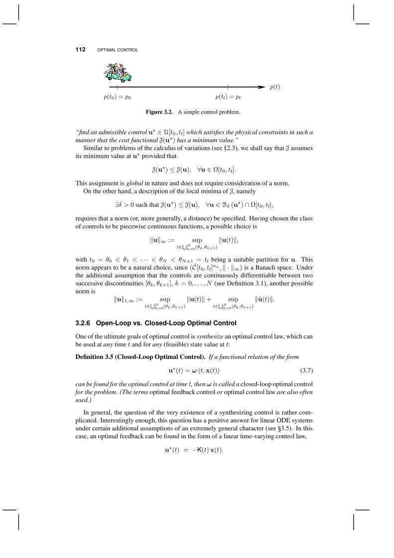
Example 3.4 (Simple Car Control Problem). Consider the control problem to drive a car,initially park at p0, to a fixed pre-assigned destination pf in a straight line (see Fig.3.2.).Here, t denotes time and p(t) represents the position of the car at a given t.
To keep the problem as simple as possible, we approximate the car by a unit point massthat can be accelerated by using the throttle or decelerated by using the brake; the controlu(t) thus represents the force on the car due to either accelerating (u(t) ≥ 0) or decelerating(u(t) ≤ 0) the car. Here, the control region U is specified as
U := u ∈ IR : uL ≤ u(t) ≤ uU,
with uL < 0 < uU , based on the acceleration and braking capabilities of the vehicle.As the state, we choose the 2-vector x(t) := (p(t), p(t)); the physical reason for using
a 2-vector is that we want to know (i) where we are, and (ii) how fast we are going. Byneglecting friction, the dynamics of our system can be expressed based on Newton’s secondlaw of motion as p(t) = u(t). Rewriting this equation in the vector form, we get
x(t) =
[
0 10 0
]
x(t) +
[
01
]
u(t). (3.5)
This is a mathematical model of the process in state form. Moreover, assuming that the carstarts from rest, we have
x(t0) =
[
p0
0
]
. (3.6)
The control problem being to bring the car at pf at rest, we impose terminal constraintsas
x(tf)−[
pf0
]
= 0.
In addition, if the car starts with G litters of gas and there are no service stations on theway, another constraints is
∫ tf
t0
[k1u(t) + k2x2(t)] dt ≤ G,
which assumes that the rate of gas consumption is proportional to both acceleration andspeed with constants of proportionality k1 and k2.
Finally, we turn to the selection of a performance measure. Suppose that the objectiveis to make the car reach point pf as quickly as possible; then, the performance measure J isgiven by
J := tf − t0 =
∫ tf
t0
dt.
An alternative criterion could be to minimize the amount of fuel expended.
3.2.5 Optimality Criteria
Having defined a performance criterion, the set of physical constraints to be satisfied, andthe set of admissible controls, one can then state the optimal control problem as follows:
112 OPTIMAL CONTROL
PSfrag replacements
p(t0) = p0 p(tf) = pf
p(t)
Figure 3.2. A simple control problem.
“find an admissible control u? ∈ U[t0, tf] which satisfies the physical constraints in such amanner that the cost functional J(u?) has a minimum value.”
Similar to problems of the calculus of variations (see 2.3), we shall say that J assumesits minimum value at u? provided that
J(u?) ≤ J(u), ∀u ∈ Ω[t0, tf].
This assignment is global in nature and does not require consideration of a norm.On the other hand, a description of the local minima of J, namely
∃δ > 0 such that J(u?) ≤ J(u), ∀u ∈ Bδ (u?) ∩ Ω[t0, tf],
requires that a norm (or, more generally, a distance) be specified. Having chosen the classof controls to be piecewise continuous functions, a possible choice is
‖u‖∞ := supt∈S
Nk=0
(θk,θk+1)
‖u(t)‖,
with t0 = θ0 < θ1 < · · · < θN < θN+1 = tf being a suitable partition for u. Thisnorm appears to be a natural choice, since (C [t0, tf]nu , ‖ · ‖∞) is a Banach space. Underthe additional assumption that the controls are continuously differentiable between twosuccessive discontinuities [θk, θk+1], k = 0, . . . , N (see Definition 3.1), another possiblenorm is
‖u‖1,∞ := supt∈
S
Nk=0
(θk,θk+1)
‖u(t)‖+ supt∈
S
Nk=0
(θk,θk+1)
‖u(t)‖.
3.2.6 Open-Loop vs. Closed-Loop Optimal Control
One of the ultimate goals of optimal control is synthesize an optimal control law, which canbe used at any time t and for any (feasible) state value at t:
Definition 3.5 (Closed-Loop Optimal Control). If a functional relation of the form
u?(t) = ω (t,x(t)) (3.7)
can be found for the optimal control at time t, thenω is called a closed-loop optimal controlfor the problem. (The terms optimal feedback control or optimal control law are also oftenused.)
In general, the question of the very existence of a synthesizing control is rather com-plicated. Interestingly enough, this question has a positive answer for linear ODE systemsunder certain additional assumptions of an extremely general character (see 3.5). In thiscase, an optimal feedback can be found in the form of a linear time-varying control law,
u?(t) = −K(t)x(t).

EXISTENCE OF AN OPTIMAL CONTROL 113
Obtaining a so-called open-loop optimal control law is much easier from a practicalviewpoint:
Definition 3.6 (Open-Loop Optimal Control). If the optimal control law is determinedas a function of time for a specified initial state value, that is,
u?(t) = ω (t,x(t0)) , (3.8)
then the optimal control is said to be in open-loop form.
Therefore, an open-loop optimal control is optimal only for a particular initial state value,whereas, if an optimal control law is known, the optimal control history can be generatedfrom any initial state. Conceptually, it is helpful to think off the difference between anoptimal control law and an open-loop optimal control as shown in Fig. 3.3. below.
PSfrag replacements
ControllerController ProcessProcess
a. Open-loop optimal control b. Closed-loop optimal control
u?(t) u?(t) x(t)x(t)
opens at t0
Figure 3.3. Open-loop vs. closed-loop optimal control.
Throughout this chapter, we shall mostly consider open-loop optimal control problems,also referred to as dynamic optimization problems in the literature. Note that open-loopoptimal controls are rarely applied directly in practice due to the presence of uncertainty(such as model mismatch, process disturbance and variation in initial condition), whichcan make the system operate sub-optimally or, worse, lead to infeasible operation due toconstraints violation. Yet, the knowledge of an open-loop optimal control law for a givenprocess can provide valuable insight on how to improve system operation as well as someidea on how much can be gained upon optimization. Moreover, open-loop optimal controlsare routinely used in a number of feedback control algorithms such as model predictivecontrol (MPC) and repeated optimization [1, 42]. The knowledge of an open-loop optimalsolution is also pivotal to many implicit optimization schemes including NCO tracking[51, 52].
3.3 EXISTENCE OF AN OPTIMAL CONTROL
Since optimal control problems encompass problems of the calculus of variations, difficul-ties are to be expected regarding the existence of a solution (see 2.4). Apart from the ratherobvious case where no feasible control exists for the problem, the absence of an optimalcontrol mostly lies in the fact that many feasible control sets of interest fail to be compact.
Observe first that when the ODEs have finite escape time for certain admissible controls,the cost functional can be unbounded. One particular sufficient condition for the solutionsof ODEs to be extended indefinitely, as given by Theorem A.52 in Appendix A.5.1, is thatthe responses satisfy an a priori bound
‖x(t;x0,u(·))‖ ≤ α, ∀t ≥ t0,
for every feasible control. In particular, the responses of a linear system x = A(t,u)x +b(t,u), from a fixed initial state, cannot have a finite escape time.

114 OPTIMAL CONTROL
Observe next that when the time interval is unbounded, the corresponding set of feasiblecontrols is itself unbounded, and hence not compact. Therefore, care should always betaken so that the operation be restricted to a compact time interval, e.g., [t0, T ], where T ischosen so large that Ω[t0, tf] 6= ∅ for some tf ∈ [t0, T ]. These considerations are illustratedin an example below.
Example 3.7. Consider the car control problem described in Example 3.4,with the objectiveto find (u(·), tf) ∈ C[t0,∞) × [t0,∞) such that pf is reached within minimal amount offuel expended:
minu(·),tf
J(u, tf) :=
∫ tf
t0
[u(t)]2 dt
s.t. Equations (3.5, 3.6)
x1(tf)− pf = 0
0 ≤ u(t) ≤ 1, ∀t.
The state trajectories being continuous and pf > p0, u(t) ≡ 0 is infeasible and J(u) > 0for every feasible control.
Now, consider the sequence of (constant) admissible controls uk(t) = 1k
, t ≥ t0, k ≥ 1.The response xk(t), t ≥ t0, is easily calculated as
x1(t) =1
2k(t− t0)2 + p0(t− t0)
x2(t) =1
k(t− t0) + p0,
and the target pf is first reached at
tkf = t0 + 4k
(
√
p20 +
2
kpf − p0
)
.
Hence, uk ∈ Ω[t0, tkf ], and we have
J(uk) =
∫ tkf
t0
1
k2dt =
4
k
(
√
p20 +
2
kpf − p0
)
−→ 0,
as k → +∞. That is, inf J(u) = 0, i.e., the problem does not have a minimum.
Even when the time horizon is finite and the system response is bounded for everyfeasible control, an optimal control may not exist. This is because, similar to problems ofthe calculus of variations, the sets of interest are too big to be compact. This is illustratedsubsequently in an example.
Example 3.8. Consider the problem to minimize the functional
J(u) :=
∫ 1
0
√
x(t)2 + u(t)2 dt,

VARIATIONAL APPROACH 115
for u ∈ C [0, 1], subject to the terminal constraint
x(1) = 1,
where the response x(t) is given by the linear initial value problem,
x(t) = u(t); x(0) = 0.
Observe that the above optimal control problem is equivalent to that of minimizing thefunctional
J(x) :=
∫ 1
0
√
x(t)2 + x(t)2 dt,
on D := x ∈ C1[0, 1] : x(0) = 0, x(1) = 1. But since this variational problem does nothave a solution (see Example 2.5, p. 68), it should be clear that the former optimal controlproblem does not have a solution either.
For a optimal control to exist, additional restrictions must be placed on the class ofadmissible controls. Two such possible classes of controls are:
(i) the class Uλ[t0, tf] ⊂ U[t0, tf] of controls which satisfy a Lipschitz condition:
‖u(t)− u(s)‖ ≤ λ‖t− s‖ ∀t, s ∈ [t0, tf];
(ii) the class Ur[t0, tf] ⊂ U[t0, tf] of piecewise constant controls with at most r points ofdiscontinuity.
Existence can also be guaranteed without restricting the controls, provided that certainconvexity assumptions hold.
3.4 VARIATIONAL APPROACH
Sufficient condition for an optimal control problem to have a solution, such as those dis-cussed in the previous section, while reassuring, are not at all useful in helping us findsolutions. In this section (and the next section), we shall describe a set of conditions whichany optimal control must necessarily satisfy. For many optimal control problems, suchconditions allow to single out a small subset of controls, sometimes even a single control.There is thus reasonable chance of finding an optimal control, if one exists, among thesecandidates. However, it should be reemphasized that necessary conditions may delineate anonempty set of candidates, even though an optimal control does not exist for the problem.
In this section, we shall consider optimal control problems having no restriction on thecontrol variables (i.e., the control region U corresponds to IRnu) as well as on the statevariables. More general optimal control problems with control and state path constraints,shall be considered later on in 3.5.
3.4.1 Euler-Lagrange Equations
We saw in 2.5.2 that the simplest problem of the calculus of variations has both its endpointsfixed. In optimal control, on the other hand, the simplest problem involves a free value of
116 OPTIMAL CONTROL
the state variables at the right endpoint (terminal time):
minimize:∫ tf
t0
`(t,x(t),u(t)) dt (3.9)
subject to: x(t) =f (t,x(t),u(t)); x(t0) = x0, (3.10)
with fixed initial time t0 and terminal time tf. A control function u(t), t0 ≤ t ≤ tf, togetherwith the initial value problem (3.10), determines the response x(t), t0 ≤ t ≤ tf (providedit exists). Thus, we may speak of finding a control, since the corresponding response isimplied.
To develop first-order necessary conditions in problems of the calculus of variations(Euler’s equation), we constructed a one-parameter family of comparison trajectoriesx(t) + ηξ(t), with ξ ∈ C1[t0, tf]
nx such that ‖ξ‖1,∞ ≤ δ (see Theorem 2.14 and proof).However, when it comes to optimal control problems such as (3.9,3.10), a variation of thestate trajectory x cannot be explicitely related to a variation of the control u, in general,because the state and control variables are implicitly related by the (nonlinear) differentialequation (3.10). Instead, we shall consider a one-parameter family of comparison trajec-tories u(t) + ηω(t), with ω ∈ C [t0, tf]nu such that ‖ω‖∞ ≤ δ. Then, analogous to theproof of Theorem 2.14, we shall use the geometric characterization for a local minimizerof a functional on a subset of a normed linear space as given by Theorem 2.13. Theseconsiderations lead to the following:
Theorem 3.9 (First-Order Necessary Conditions). Consider the problem to minimize thefunctional
J(u) :=
∫ tf
t0
`(t,x(t),u(t)) dt, (3.11)
subject to
x(t) =f(t,x(t),u(t)); x(t0) = x0, (3.12)
for u ∈ C [t0, tf]nu , with fixed endpoints t0 < tf, where ` and f are continuous in (t,x,u)and have continuous first partial derivatives with respect to x and u for all (t,x,u) ∈[t0, tf]× IRnx × IRnu . Suppose that u? ∈ C [t0, tf]nu is a (local) minimizer for the problem,and letx? ∈ C1[t0, tf]
nx denote the corresponding response. Then, there is a vector functionλ? ∈ C1[t0, tf]
nx such that the triple (u?,x?,λ?) satisfies the system
x(t) =f(t,x(t),u(t)); x(t0) =x0 (3.13)
λ(t) =− `x(t,x(t),u(t))− fx(t,x(t),u(t))Tλ(t); λ(tf) =0 (3.14)
0 =`u(t,x(t),u(t)) + fu(t,x(t),u(t))Tλ(t). (3.15)
for t0 ≤ t ≤ tf. These equations are known collectively as the Euler-Lagrange equations,and (3.14) is often referred to as the adjoint equation (or the costate equation).
Proof. Consider a one-parameter family of comparison controls v(t; η) := u?(t)+ ηω(t),whereω(t) ∈ C [t0, tf]nu is some fixed function, and η is a (scalar) parameter. Based on thecontinuity and differentiability properties of f , we know that there exists η > 0 such that theresponse y(t; η) ∈ C1[t0, tf]
nx associated to v(t; η) through (3.12) exists, is unique, and isdifferentiable with respect to η, for all η ∈ Bη (0) and for all t ∈ [t0, tf] (see Appendix A.5).Clearly, η = 0 provides the optimal response y(t; 0) ≡ x?(t), t0 ≤ t ≤ tf.

VARIATIONAL APPROACH 117
Since the control v(t; η) is admissible and its associated response is y(t, η), we have
J(v(·; η)) =
∫ tf
t0
[
`(t,y(t; η),v(t; η)) + λ(t)T[f(t,y(t; η),v(t; η)) − y(t; η)]
]
dt
=
∫ tf
t0
[
`(t,y(t; η),v(t; η)) + λ(t)Tf(t,y(t; η),v(t; η)) + λ(t)
Ty(t; η)
]
dt
− λ(tf)Ty(tf; η) + λ(t0)
Ty(t0; η),
for any λ ∈ C1[t0, tf]nx and for each η ∈ Bη (0). Based on the differentiability properties
of ` and y, and by Theorem 2.A.59, we have
∂
∂ηJ(v(·; η)) =
∫ tf
t0
[
`u(t,y(t; η),v(t; η)) + fu(t,y(t; η),v(t; η))Tλ(t)
]Tω(t) dt
+
∫ tf
t0
[
`x(t,y(t; η),v(t; η)) + fx(t,y(t; η),v(t; η))Tλ(t) + λ(t)
]Tyη(t; η) dt
− λ(tf)Tyη(tf; η) + λ(t0)
Tyη(t0; η),
for any ω ∈ C [t0, tf]nu and any λ ∈ C1[t0, tf]nx . Taking the limit as η → 0, and since
yη(t0; η) = 0, we get
δJ(u?;ω) =
∫ tf
t0
[
`u(t,x?(t),u?(t)) + fu(t,x?(t),u?(t))Tλ(t)
]Tω(t) dt
+
∫ tf
t0
[
`x(t,x?(t),u?(t)) + fx(t,x?(t),u?(t))Tλ(t) + λ(t)
]Tyη(t; 0) dt
− λ(tf)Tyη(tf; 0),
which is finite for each ω ∈ C [t0, tf]nu and each λ ∈ C1[t0, tf]nx , since the integrand
is continuous on [t0, tf]. That is, δJ(u?;ω) exists for each ω ∈ C [t0, tf]nu and eachλ ∈ C1[t0, tf]
nx .Now, u? being a local minimizer, by Theorem 2.13,
0 =
∫ tf
t0
[
`?x + f?xTλ(t) + λ(t)
]Tyη(t; 0) +
[
`?u + f?uTλ(t)
]Tω(t) dt− λ(tf)
Tyη(tf; 0),
for each ω ∈ C [t0, tf]nu and each λ ∈ C1[t0, tf]nx , where the compressed notations `?z :=
`z(t,x?(t),u?(t)) and f?z := fz(t,x
?(t),u?(t)) are used.Because the effect of a variation of the control on the course of the response is hard
to determine (i.e., yη(t; 0)), we choose λ?(t), t0 ≤ t ≤ tf, so as to obey the differentialequation
λ(t) =− f?xTλ(t)− `?x, (3.16)
with the terminal conditionλ(tf) = 0. Note that (3.16) being a linear system of ODEs, andfrom the regularity assumptions on ` and f , the solution λ? exists and is unique over [t0, tf](see Theorem A.50, p. xiv), i.e., λ ∈ C1[t0, tf]
nx . That is, the condition
0 =
∫ tf
t0
[
`?u + f?uTλ?(t)
]Tω(t) dt,

118 OPTIMAL CONTROL
must hold for anyω ∈ C [t0, tf]nu . In particular, forω(t) such thatωi(t) := `?ui+f?uiTλ?(t)
and ωj(t) = 0 for j 6= i, we get
0 =
∫ tf
t0
[
`?ui + f?uiTλ?(t)
]2
dt,
for each i = 1, . . . , nx, which in turn implies the necessary condition that
0 = `ui(t,x?(t),u?(t)) + fui(t,x
?(t),u?(t))Tλ?(t), i = 1, . . . , nx,
for each t ∈ [t0, tf].
Some comments are in order before we look at an example.
The optimality conditions consist of nu algebraic equations (3.15), together with2 × nx ODEs (3.13,3.14) and their respective boundary conditions. Hence, theEuler-Lagrange equations provide a complete set of necessary conditions. However,the boundary conditions for (3.13) and (3.14) are split, i.e., some are given at t = t0and others at t = tf. Such problems are known as two-point boundary value problems(TPBVPs) and are notably more difficult to solve than IVPs.
In the special case where f(t,x(t),u(t)) := u(t), with nu = nx, (3.15) gives
λ?(t) = −`u(t,x?(t),u?(t)).
Then, from (3.14), we obtain the Euler equation
ddt`u(t,x?(t), x?(t)) = `x(t,x?(t), x?(t)),
together with the natural boundary condition
[`u(t,x?(t), x?(t))]t=tf= 0.
Hence, the Euler-Lagrange equations encompass the necessary conditions of opti-mality derived previously for problems of the calculus of variations (see 2.5).
It is convenient to introduce the Hamiltonian functionH : IR× IRnx× IRnu× IRnx →IR associated with the optimal control problem (3.9,3.10), by adjoining the right-handside of the differential equations to the cost integrand as
H(t,x,u,λ) = `(t,x,u) + λTf(t,x,u). (3.17)
Thus, Euler-Lagrange equations (3.13–3.15) can be rewritten as
x(t) = Hλ; x(t0) = x0 (3.13’)
λ(t) = −Hx; λ(tf) = 0 (3.14’)0 = Hu, (3.15’)
for t0 ≤ t ≤ tf. Note that a necessary condition for the triple (u?,x?,λ?) to give alocal minimum of J is that u?(t) be a stationary point of the Hamiltonian functionwith x?(t) and λ?(t), at each t ∈ [t0, tf]. In some cases, one can express u(t) as a

VARIATIONAL APPROACH 119
function of x(t) and λ(t) from (3.15’), and then substitute into (3.13’,3.14’) to get aTPBVP in the variables x and λ only (see Example 3.10 below).
The variation of the Hamiltonian function along an optimal trajectory is given by
ddtH = Ht +HT
xx +HTuu + fTλ = Ht +HT
uu + fT[
Hx + λ]
= Ht.
Hence, if neither ` nor f depend explicitly on t, we get ddtH ≡ 0, henceH is constant
along an optimal trajectory; in other words, H yields a first integral to the TPBVP(3.13’–3.15’).
The Euler-Lagrange equations (3.13’–3.15’) are necessary conditions both fora minimization and for a maximization problem. Yet, in a minimiza-tion problem, u?(t) must minimize H(t,x?(t), ·,λ?(t)), i.e., the conditionHuu(t,x?(t),u?(t),λ?(t)) ≥ 0 is also necessary. On the other hand, the additionalconditionHuu(t,x?(t),u?(t),λ?(t)) ≤ 0 is necessary in a maximization problem.These latter conditions have not yet been established and shall be discussed later on.
Example 3.10. Consider the optimal control problem
minimize: J(u) :=
∫ 1
0
[
12u(t)
2 − x(t)]
dt (3.18)
subject to: x(t) = 2 [1− u(t)] ; x(0) = 1. (3.19)
To find candidate optimal controls for the problem (3.18,3.19), we start by forming theHamiltonian function
H(x, u, λ) = 12u
2 − x+ 2λ(1− u).Candidate solutions (u?, x?, λ?) are those satisfying the Euler-Lagrange equations, i.e.,
x?(t) = Hλ = 2 [1− u?(t)] ; x?(0) = 1
λ?(t) = −Hx = 1; λ?(1) = 0
0 = Hu = u?(t)− 2λ?(t).
The adjoint equation trivially yields
λ?(t) = t− 1,
and from the optimality condition, we get
u?(t) = 2(t− 1).
(Note that u? is indeed a candidate minimum solution for the problem since Huu = 1 > 0for each 0 ≤ t ≤ 1.) Finally, substituting the optimal control candidate back into (3.19)yields
x?(t) = 6− 4t; x?(0) = 1.
Integrating the latter equation, and drawing the results together, we obtain
u?(t) = 2(t− 1) (3.20)
x?(t) = − 2t2 + 6t+ 1 (3.21)λ?(t) = t− 1. (3.22)

120 OPTIMAL CONTROL
It is also readily verified that H is constant along the optimal trajectory,
H(t, x?(t), u?(t), λ?(t)) = −5.
Finally, we illustrate the optimality of the controlu? by considering the modified controlsv(t; η) := u?(t)+ηω(t), and their associated responses y(t; η). The perturbed cost functionreads:
J(v(t; η)) :=
∫ 1
0
[
1
2[u?(t) + ηω(t)]2 − y(t; η)
]
dt
s.t. y(t; η) = 2 [1− u?(t)− ηω(t)] ; x(0) = 1.
The cost function J(v(t; η)) is represented in Fig. 3.4. for different perturbationsω(t) = tk,k = 0, . . . , 4. Note that the minimum of J(v(t; η)) is always attained at η = 0.
-2.667
-2.6665
-2.666
-2.6655
-2.665
-2.6645
-2.664
-2.6635
-2.663
-2.6625
-2.662
-2.6615
-0.1 -0.05 0 0.05 0.1
PSfrag replacements
η
J(v
(t;η
))
ω(t) = 1
ω(t) = t
ω(t) = t2
ω(t) = t3
ω(t) = t4
Figure 3.4. Function J(v(t; η)) for various perturbations ω(t) = tk, k = 0, . . . , 4, inExample 3.10.
3.4.2 Mangasarian Sufficient Conditions
In essence, searching for a control u? that minimizes the performance measure J meansthat J(u?) ≤ J(u), for all admissible u. That is, what we want to determine is the globalminimum value of J, not merely local minima. (Remind that there may actually be severalglobal optimal controls, i.e., distinct controls achieving the global minimum of J.) Condi-tions under which the necessary conditions (3.13’–3.15’) are also sufficient for optimality,i.e., provide a global optimal control are given by the following:
Theorem 3.11 (Mangasarian Sufficient Condition). Consider the problem to minimizethe functional
J(u) :=
∫ tf
t0
`(t,x(t),u(t)) dt, (3.23)
subject to
x(t) =f(t,x(t),u(t)); x(t0) = x0, (3.24)

VARIATIONAL APPROACH 121
for u ∈ C [t0, tf]nu , with fixed endpoints t0 < tf, where ` and f are continuous in (t,x,u),have continuous first partial derivatives with respect to x and u, and are [strictly] jointlyconvex in x and u, for all (t,x,u) ∈ [t0, tf] × IRnx × IRnu . Suppose that the tripleu? ∈ C [t0, tf]nu , x? ∈ C1[t0, tf]
nx and λ? ∈ C1[t0, tf]nx satisfies the Euler-Lagrange
equations (3.13–3.15). Suppose also that
λ?(t) ≥ 0, (3.25)
for all t ∈ [t0, tf]. Then, u? is a [strict] global minimizer for the problem (3.23,3.24).
Proof. ` being jointly convex in (x,u), for any feasible controluand its associated responsex, we have
J(u)− J(u?) =
∫ tf
t0
[`(t,x(t),u(t)) − `(t,x?(t),u?(t))] dt
≥∫ tf
t0
(
`?xT [x(t)− x?(t)] + `?u
T [u(t)− u?(t)])
dt,
with the usual compressed notation. Since the triple (u?,x?,λ?) satisfies the Euler-Lagrange equations (3.13–3.15), we obtain
J(u)− J(u?) ≥∫ tf
t0
(
−[
f?xTλ?(t) + λ
?(t)]T
[x(t) − x?(t)]
−[
f?uTλ?(t)
]T[u(t)− u?(t)]
)
dt,
Integrating by part the term in λ?(t), and rearranging the terms, we get
J(u)− J(u?) ≥∫ tf
t0
λ?(t)T(f(t,x(t),u(t))− f (t,x?(t),u?(t))− f ?x [x(t)− x?(t)]
−f?u [u(t)− u?(t)]) dt
− λ?(tf)T[x(tf)− x?(tf)] + λ?(t0)
T[x(t0)− x?(t0)] .
Note that the integrand is positive due to (3.25) and the joint convexity of f in (x,u); theremaining two terms are equal to zero due to the optimal adjoint boundary conditions andthe prescribed state initial conditions, respectively. That is,
J(u) ≥ J(u?),
for each feasible control.
Remark 3.12. In the special case where f is linear in (x,u), the result holds without anysign restriction for the costatesλ?(t). Further, if ` is jointly convex in (x,u) andϕ is convexin x, while f is jointly concave in (x,u) and λ?(t) ≤ 0, then the necessary conditions arealso sufficient for optimality.
Remark 3.13. The Mangasarian sufficient conditions have limited applicability for, in mostpractical problems, either the terminal cost, the integral cost, or the differential equationsfail to be convex or concave. 2
2A less restrictive sufficient condition, known as the Arrow sufficient condition, ’only’ requires that the functionM(t,x, λ?) := minu∈U H(t,x,u,λ?), i.e., the minimized Hamiltonian with respect to u ∈ U , be a convexfunction in x. See, e.g., [49] for a survey of sufficient conditions in optimal control theory.
122 OPTIMAL CONTROL
Example 3.14. Consider the optimal control problem (3.18,3.19) in Example 3.10. The in-tegrand is jointly convex in (u, x) on IR2, and the right-hand side of the differential equationis linear in u (and independent of x). Moreover, the candidate solution (u?(t), x?(t), λ?)given by (3.20–3.22) satisfies the Euler-Lagrange equations (3.13–3.15), for each t ∈ [0, 1].Therefore,u?(t) is a global minimizer for the problem (irrespective of the sign of the adjointvariable due to the linearity of (3.19), see Remark 3.12).
3.4.3 Piecewise Continuous Extremals
It may sometimes occur that a continuous control u ∈ C [t0, tf]nu satisfying the Euler-Lagrange equations cannot be found for a particular optimal control problem. It is thennatural to wonder whether such problems have extremals in the larger class of piecewisecontinuous controls C [t0, tf]nu (see Definition 3.1). It is also natural to seek improvedresults in the class of piecewise continuous controls, even though a continuous controlsatisfying the Euler-Lagrange equations could be found. Discontinuous controls give riseto discontinuities in the slope of the response (i.e., x ∈ C1[t0, tf]), and are referred toas corner points (or simply corners) by analogy to classical problems of the calculus ofvariations (see 2.6). The purpose of this subsection is to summarize the conditions thatmust hold at the corner points of an optimal solution.
Consider an optimal control problem of the form (3.9,3.10), and suppose that u? ∈C [t0, tf] is an optimal control for that problem, with associated response x? and adjoint λ
?.
Then, at every possible corner point θ ∈ (t0, tf) of u?, we have
x?(θ−) = x?(θ+) (3.26)
λ?(θ−) = λ
?(θ+) (3.27)
H(θ−, x?(θ), u?(θ−), λ?(θ)) = H(θ+, x?(θ), u?(θ+), λ
?(θ)), (3.28)
where θ− and θ+ denote the time just before and just after the corner, respectively; z(θ−)and z(θ+) denote the left and right limit values of a quantity z at θ, respectively.
Remark 3.15 (Link to the Weierstrass-Erdmann Corner Conditions). It is readilyshown that the corner conditions (3.27)and (3.28)are equivalent to the Weierstrass-Erdmannconditions (2.23) and (2.24) in classical problems of the calculus of variations.
Although corners in optimal control trajectories are more common in problems hav-ing inequality path constraints (either input or state constraints), the following exampleillustrates that problems without path inequality constraint may also exhibit corners.
Example 3.16. Consider the optimal control problem
minimize: J(u) :=
∫ 1
0
[
u(t)2 − u(t)4 − x(t)]
dt (3.29)
subject to: x(t) = −u(t); x(0) = 1 (3.30)
The Hamiltonian function for this problem reads
H(x, u, λ) = u2 − u4 − x− λu.

VARIATIONAL APPROACH 123
Candidate optimal solutions (u?, x?, λ?) are those satisfying the Euler-Lagrange equations
x(t) = Hλ = u(t); x(0) = 1
λ(t) = −Hx = 1; λ?(1) = 0 (3.31)
0 = Hu = 2u(t)− 4u(t)3 − λ(t). (3.32)
The adjoint equation (3.31) has solution λ?(t) = t−1, 0 ≤ t ≤ 1, which upon substitutioninto (3.32) yields
2u?(t)− 4u?(t)3 = t− 1.
Values of the control variable u(t), 0 ≤ t ≤ 1, satisfying the former condition are shownin Fig. 3.16 below. Note that for there is a unique solution u1(t) to the Euler-Lagrangeequations for 0 ≤ t / 0.455, then 3 possible solutions u1(t), u2(t), and u3(t) exist for0.455 / t ≤ 1. That is, candidate optimal controls start with the value u?(t) = u1(t) untilt ≈ 0.455. Then, the optimal control may be discontinuous and switch between u1(t),u2(t), and u3(t). Note, however, that a discontinuity can only occur at those time instantswhere the corner condition (3.28) is satisfied.
-1
-0.5
0
0.5
1
0 0.2 0.4 0.6 0.8 1
PSfrag replacements
t
u(t
)
Hu(t, u(t), λ?(t)) = 0
u1(t)
u2(t)
u3(t)
t≈
0.4
55
Figure 3.5. Values of the control variable u(t), 0 ≤ t ≤ 1, satisfying the Euler-Lagrange equationsin Example 3.16.
3.4.4 Interpretation of the Adjoint Variables
We saw in Chapter 1 on nonlinear programming that the Lagrange multiplier associatedto a particular constraint can be interpreted as the sensitivity of the objective function to achange in that constraint (see Remark 1.61, p. 30). Our objective in this subsection is toobtain a useful interpretation of the adjoint variables λ(t) which are associated to the statevariables x(t).
Throughout this subsection, we consider an optimal control problem of the followingform
minimize: J(u) =
∫ tf
t0
`(t,x(t),u(t)) dt (3.33)
subject to: x(t) = f(t,x(t),u(t)); x(t0) = x0, (3.34)
124 OPTIMAL CONTROL
with fixed initial time t0 and terminal time tf, where ` and f are continuous in (t,x,u),and have continuous first partial derivatives with respect to x and u, for all (t,x,u) ∈[t0, tf]× IRnx × IRnu . Let V(x0, t0) denote the minimum value of J(u), for a given initialstate x0 at t0. For simplicity, suppose that u? ∈ C [t0, tf]nu is the unique control providingthis minimum, and let x? ∈ C1[t0, tf]
nx and λ? ∈ C1[t0, tf]nx denote the corresponding
response and adjoint trajectories, respectively.Now, consider a modification of the optimal control problem (3.33,3.34) in which the
initial state is x0 + ξ, with ξ ∈ IRnx . Suppose that a unique optimal control, v(t; ξ), existsfor the perturbed problem for each ξ ∈ Bδ (0), with δ > 0, and let y(t; ξ) denote thecorresponding optimal response, i.e.,
y(t; ξ) = f(t,y(t; ξ),v(t; ξ)); y(t0; ξ) = x0 + ξ.
Clearly, v(t;0) = u?(t) and y(t;0) = x?(t), for t0 ≤ t ≤ tf. Suppose further that thefunctions v(t; ξ) and y(t; ξ) are continuously differentiable with respect to ξ on Bδ (0).
Appending the differential equation (3.34) in (3.33) with the adjoint variable λ?, wehave
V(y(t0; ξ), t0) :=
∫ tf
t0
`(t,y(t; ξ),v(t; ξ)) dt
=
∫ tf
t0
(
`(t,y(t; ξ),v(t; ξ)) + λ?(t)T[f(t,y(t; ξ),v(t; ξ))− y(t; ξ)]
)
dt.
Then, upon differentiation of V(x0 + ξ, t0) with respect to ξ, we obtain
∂
∂ξV(y(t0; ξ), t0) =
∫ tf
t0
[
`u(t,y(t; ξ),v(t; ξ)) + λ?(t)Tfu(t,y(t; ξ),v(t; ξ))
]Tvξ(t; ξ) dt
+
∫ tf
t0
[
`x(t,y(t; ξ),v(t; ξ)) + λ?(t)Tfx(t,y(t; ξ),v(t; ξ)) + λ
?(t)]T
yξ(t; ξ) dt
− λ?(tf)Tyξ(tf; ξ) + λ?(t0)
Tyξ(t0; ξ),
and taking the limit as ξ → 0 yields
∂
∂ξV(v(t0;ξ), t0)
∣
∣
∣
∣
ξ=0
=
∫ tf
t0
[
`u(t,x?(t),u?(t)) + λ?(t)Tfu(t,x?(t),u?(t))
]Tvξ(t;0) dt
+
∫ tf
t0
[
`x(t,x?(t),u?(t)) + λ?(t)Tfx(t,x?(t),u?(t)) + λ
?(t)]T
yξ(t;0) dt
− λ?(tf)Tyξ(tf;0) + λ?(t0)
Tyξ(t0;0).
Finally, noting that the triple (u?,x?,λ?) satisfies the Euler-Lagrange equations (3.13–3.15), and since v(t0; ξ) = Inx , we are left with
λ?(t0) =∂
∂ξV(v(t0; ξ), t0)
∣
∣
∣
∣
ξ=0
= Vx(x0, t0). (3.35)
That is, the adjoint variable λ(t0) at initial time can be interpreted as the sensitivity of thecost functional to a change in the initial condition x0. In other words, λ(t0) represents themarginal valuation in the optimal control problem of the state at initial time.
VARIATIONAL APPROACH 125
The discussion thus far has only considered the adjoint variables at initial time. We shallnow turn to the interpretation of the adjoint variables λ(t) at any time t0 ≤ t ≤ tf. Westart by proving the so-called principle of optimality, which asserts that any restriction on[t1, tf] of an optimal control on [t0, tf] is itself optimal, for any t1 ≥ t0.
Lemma 3.17 (Principle of Optimality). Let u? ∈ C [t0, tf]nu be an optimal control for theproblem to
minimize:∫ tf
t0
`(t,x(t),u(t)) dt (3.36)
subject to: x(t) = f(t,x(t),u(t)); x(t0) = x0, (3.37)
and let x? ∈ C1[t0, tf]nx denote the corresponding optimal response. Then, for any t1 ∈
[t0, tf], the restriction u?(t), t1 ≤ t ≤ tf, is an optimal control for the problem to
minimize:∫ tf
t1
`(t,x(t),u(t)) dt (3.38)
subject to: x(t) = f(t,x(t),u(t)); x(t1) = x?(t1). (3.39)
Proof. Let V(x0, t0) denote the minimum values of the optimal control problem (3.36,3.37).Clearly,
V(x0, t0) =
∫ t1
t0
`(t,x?(t),u?(t)) dt+∫ tf
t1
`(t,x?(t),u?(t)) dt.
By contradiction, suppose that the restriction u?(t), t1 ≤ t ≤ tf, is not optimal for theproblem (3.38,3.39). Then, there exists a (feasible) control u†(t), t1 ≤ t ≤ tf, that impartsto the functional (3.38) the value
∫ tf
t1
`(t,x†(t),u†(t)) dt <∫ tf
t1
`(t,x?(t),u?(t)) dt.
Further, by joining u?(t), t0 ≤ t ≤ t1, and u†(t), t1 ≤ t ≤ tf, one obtains a piecewisecontinuous control that is feasible and satisfies
∫ t1
t0
`(t,x?(t),u?(t)) dt+
∫ tf
t1
`(t,x†(t),u†(t)) dt < V(x0, t0),
hence contradicting the optimality of u?, t0 ≤ t ≤ tf, for the problem (3.36,3.37).
Back to the question of the interpretation of the adjoint variables, the method used to reach(3.35) at initial time can be applied to the restricted optimal control problem (3.38,3.39),which by Lemma 3.17 has optimal solution u?(t), t1 ≤ t ≤ tf. This method leads to theresult
λ?(t1) = Vx(x?(t1), t1),
and since the time t1 was arbitrary, we get
λ?(t) = Vx(x?(t), t), t0 ≤ t ≤ tf.
That is, if there were an exogenous, tiny perturbation to the state variable at time t and if thecontrol were modified optimally thereafter, the optimal cost value would change at the rate

126 OPTIMAL CONTROL
λ(t); said differently, λ(t) is the marginal valuation in the optimal control problem of thestate variable at time t. In particular, the optimal cost value remains unchanged in case ofan exogenous perturbation at terminal time tf, i.e., the rate of change is Vx(x?(tf), tf) = 0.This interpretation confirms the natural boundary conditions of the adjoint variables in theEuler-Lagrange equations (3.13–3.15).
3.4.5 General Terminal Constraints
So far, we have only considered optimal control problems with fixed initial time t0 andterminal time tf, and free terminal state variables x(tf). However, many optimal controlproblems do not fall into this formulation. Often, the terminal time is free (e.g., in minimumtime problems), and the state variables at final time are either fixed or constrained to lie ona smooth manifold.
In this subsection, we shall consider problems having end-point constraints of the formψ(tf,x(tf)) = 0, with tf being specified or not. Besides terminal constraints, we shall alsoadd a terminal cost (or salvage term) φ(tf,x(tf)) to the cost functional, so that the problemis now in the Bolza form. In the case of a free terminal time problem, tf shall be consideredan additional variable in the optimization problem. Similar to free end-point problems ofthe calculus of variations (see, e.g., 2.5.5 and 2.7.3), we shall then define the optimizationhorizon by extension on a “sufficiently” large interval [t0, T ], and consider the linear spaceC [t0, T ]nu× IR, supplied with the norm ‖(u, t)‖∞ := ‖u‖∞+ |t|, as the class of admissiblecontrols for the problem.
In order to obtain necessary conditions of optimality for problems with terminal con-straints, the idea is to apply the method of Lagrange multipliers described in 2.7.1, byspecializing the normed linear space (X, ‖ · ‖) to (C [t0, T ]nu × IR, ‖(·, ·)‖∞) and consid-ering the Gateaux derivative δJ(u, tf;ω, τ) at any point (u, tf) and in any direction (ω, τ).One such set of necessary conditions is given by the following:
Theorem 3.18 (Necessary Conditions for Problems having Equality Terminal Con-straints). Consider the optimal control problem to
minimize: J(u, tf) :=
∫ tf
t0
`(t,x(t),u(t)) dt+ φ(tf,x(tf)) (3.40)
subject to: Pk(u, tf) := ψk(tf,x(tf)) = 0, k = 1, . . . , nψ (3.41)x(t) = f(t,x(t),u(t)); x(t0) = x0, (3.42)
for u ∈ C [t0, T ]nu , with fixed initial time t0 and free terminal time tf; ` and f are continuousin (t,x,u) and have continuous first partial derivatives with respect to x and u for all(t,x,u) ∈ [t0, T ]× IRnx × IRnu ; φ andψ are continuous and have continuous first partialderivatives with respect to t and x for all (t,x) ∈ [t0, T ]× IRnx . Suppose that (u?, t?f ) ∈C [t0, T ]nu× [t0, T ) is a (local) minimizer for the problem, and let x? ∈ C1[t0, T ]nx denotethe corresponding response. Suppose further that
∣
∣
∣
∣
∣
∣
∣
δP1(u?, t?f ; ω1, τ1) · · · δP1(u
?, t?f ; ωnψ , τnψ )...
. . ....
δPnψ (u?, t?f ; ω1, τ1) · · · δPnψ(u?, t?f ; ωnψ , τnψ )
∣
∣
∣
∣
∣
∣
∣
6= 0, (3.43)
for nψ (independent) directions (ω1, τ1), . . . , (ωnψ , τnψ ) ∈ C [t0, T ]nu × IR. Then, thereexist a function λ? ∈ C1[t0, T ]nx and a vector ν? ∈ IRnψ such that (u?,x?,λ?,ν?, t?f )

VARIATIONAL APPROACH 127
satisfies the Euler-Lagrange equations
x(t) =Hλ(t,x(t),u(t),λ(t)); x(t0) = x0 (3.44)
λ(t) = −Hx(t,x(t),u(t),λ(t)); λ(tf) = Φx(tf,x(tf)) (3.45)0 =Hu(t,x(t),u(t),λ(t)), (3.46)
for all t0 ≤ t ≤ tf, along with the conditions
ψ(tf,x(tf)) = 0 (3.47)Φt(tf,x(tf)) +H(tf,x(tf),u(tf),λ(tf)) = 0, (3.48)
with Φ := φ+ νTψ andH := `+ λTf .
Proof. Consider a one-parameter family of comparison controls v(t; η) := u?(t)+ ηω(t),whereω(t) ∈ C [t0, T ]nu is some fixed function, and η is a (scalar) parameter. Let y(t; η) ∈C1[t0, T ]nx be the response corresponding to v(t; η) through (3.42). In particular, η = 0provides the optimal response y(t; 0) ≡ x?(t), t0 ≤ t ≤ tf.
We show, as in the proof of Theorem 3.9, that the Gateaux variation at (u?, t?f ) in anydirection (ω, τ) ∈ C [t0, T ]nu × IR of the cost functional J subject to the initial valueproblem (3.42) is given by
δJ(u?, t?f ;ω, τ) =
∫ t?f
t0
[
`u(t,x?(t),u?(t)) + fu(t,x?(t),u?(t))Tλ(0)(t)
]Tω(t) dt
+[
φt(t?f ,x
?(t?f )) + `(t?f ,x?(t?f ),u?(t?f )) + f(t?f ,x
?(t?f ),u?(t?f ))
Tλ(0)(t)
]
τ,
with the adjoint variables λ(0)(t), t0 ≤ t ≤ t?f , calculated as
λ(0)
(t) =− `x(t,x?(t),u?(t)) − fx(t,x?(t),u?(t))Tλ(0)(t); λ(0)(t?f ) = φx(t?f ,x
?(t?f )).
On the other hand, the Gateaux variations at (u?, t?f ) in any direction (ω, τ) ∈C [t0, T ]nu × IR of the functionals Pk subject to the initial value problem (3.42) is given by
δPk(u?, t?f ;ω, τ) =
∫ t?f
t0
[
fu(t,x?(t),u?(t))Tλ(k)(t)
]Tω(t) dt
+[
(ψk)t(t?f ,x
?(t?f )) + f(t?f ,x?(t?f ),u?(t?f ))
Tλ(k)(t)
]
τ,
with the adjoint variables λ(k)(t), t0 ≤ t ≤ t?f , given by
λ(k)
(t) =− fx(t,x?(t),u?(t))Tλ(k)(t); λ(k)(t?f ) = (ψk)x(t?f ,x
?(t?f )), (3.49)
for each k = 1, . . . , nψ.Note that, based on the differentiability assumptions on `, φ, ψ and f , the Gateaux
derivatives δJ(u?, t?f ;ω, τ) and δPk(u?, t?f ;ω, τ) exist and are continuous in each direction(ω, τ) ∈ C [t0, T ]nu × IR. Since (u?, t?f ) gives a (local) minimum for (3.40–3.42) andcondition (3.43) holds at (u?, t?f ), by Theorem 2.47 (and Remark 2.49), there exists avector ν? ∈ IRnψ such that
0 = δ(
J +∑nψ
k=1ν?kPk
)
(u?, t?f ; ξ, τ)
=
∫ t?f
t0
Hu(t,x?(t),u?(t),λ?(t))Tω(t) dt
+ [Φt(t?f ,x
?(t?f )) +H(t?f ,x?(t?f ),u?(t?f ),λ?(t?f ))] τ,

128 OPTIMAL CONTROL
for each (ω, τ) ∈ C [t0, T ]nu × IR, where Φ := φ + ν?Tψ, λ? := λ(0) +∑nψ
k=1 ν?kλ
(k),and H := ` + λ?
Tf . In particular, taking τ := 0 and restricting attention to ω(t) such
that ωi(t) := Hui(t,x?(t),u?(t),λ?(t)) and ωj(t) := 0 for j 6= i, we get the necessaryconditions of optimality
Hui(t,x?(t),u?(t),λ?(t)) = 0, i = 1, . . . , nx,
for each t0 ≤ t ≤ t?f . On the other hand, choosing ω(t) := 0, t0 ≤ t ≤ t?f , andτ := Φt(t
?f ,x
?(t?f )) +H(t?f ,x?(t?f ),u
?(t?f ),λ?(t?f )), yields the transversal condition
Φt(t?f ,x
?(t?f )) +H(t?f ,x?(t?f ),u
?(t?f ),λ?(t?f )) = 0.
Finally, since the adjoint differential equations giving λ(0) and λ(k), k = 1, . . . , nψ, arelinear, the adjoint variables λ? must satisfy the following differential equations and corre-sponding terminal conditions
λ?(t) = −Hx(t,x?(t),u?(t),λ?(t)); λ?(t?f ) = Φx(t?f ,x
?(t?f )),
for all t0 ≤ t ≤ t?f .
Observe that the optimality conditions consist of nu algebraic equations (3.46), togetherwith 2×nxODEs (3.44,3.45) and their respective boundary conditions,which determine theoptimal control u?, response x?, and adjoint trajectories λ?. Here again, these equationsyield a challenging TPBVP. In addition, the necessary conditions (3.47) determine theoptimal Lagrange multiplier vector ν?. Finally, for problems with free terminal time,the transversal condition (3.48) determines the optimal terminal time t?f . We thus have acomplete set of necessary conditions.
Remark 3.19 (Reachability Condition). One of the most difficult aspect in applyingTheorem 3.18 is to verify that the terminal constraints satisfy the regularity condition (3.43).In order to gain insight into this condition, consider an optimal control problem of the form(3.40–3.42), with fixed terminal time tf and a single terminal state constraint P(u) :=xj(tf) − xfj = 0, for some j ∈ 1, . . . , nx. The Gateaux variation of P at u? in anydirection ω ∈ C [t0, tf]nu is
δP(u?;ω) =
∫ tf
t0
[
fu(t,x?(t),u?(t))Tλ(j)(t)
]Tω(t) dt,
where λ(j)
(t) = −fx(t,x?(t),u?(t))Tλ(j)(t), t0 ≤ t ≤ tf, with terminal conditions
λ(j)j (tf) = 1 and λ(j)
i (tf) = 0 for i 6= j. By choosing ω(t) := fu(t,x?(t),u?(t))Tλ(j)(t),
t0 ≤ t ≤ tf, we obtain the following sufficient condition for the terminal constraint to beregular:
∫ tf
t0
λ(j)(t)Tfu(t,x?(t),u?(t))fu(t,x?(t),u?(t))
Tλ(j)(t) dt 6=0. (3.50)
This condition can be seen as a reachability condition3 for the system. In other words, ifthis condition does not hold, then it may not be possible to find a control u(t) so that theterminal condition xj(tf) = xfj be satisfied at final time.
3Reachability is defined as follow (see, e.g., [2]):
Definition 3.20 (Reachability). A state xf is said to be reachable at time tf, if for some finite t0 < tf there existsan input u(t), t0 ≤ t ≤ tf, that transfers the state x(t) from the origin at t0, to xf at time tf.
VARIATIONAL APPROACH 129
More generally, for optimal control problems such as (3.40–3.42) with fixed terminal timetf and nψ terminal constraints ψk(x(tf)) = 0, the foregoing sufficient condition becomes
rankΨ = nψ,
where Ψ is a (nψ × nψ) matrix defined by
Ψij :=
∫ tf
t0
λ(i)(t)Tfu(t,x?(t),u?(t))fu(t,x?(t),u?(t))
Tλ(j)(t) dt, 1 ≤ i, j ≤ nψ,
with the adjoint variables λ(k)(t), t0 ≤ t ≤ tf, defined by (3.49).
A summary of the necessary conditions of optimality encountered so far is given here-after, before an example is considered.
Remark 3.21 (Summary of Necessary Conditions). Necessary conditions of optimalityfor the problem
minimize:∫ tf
t0
`(t,x(t),u(t)) dt+ φ(tf,x(tf))
subject to: ψ(tf,x(tf)) = 0,
x(t) = f (t,x(t),u(t)); x(t0) = x0,
are as follows:
Euler-Lagrange Equations:
x = Hλ
λ = −Hx
0 = Hu
, t0 ≤ t ≤ tf;
withH := `+ λTf .
Legendre-Clebsch Condition:
Huu semi-definite positive, t0 ≤ t ≤ tf;
Transversal Conditions:[
H + φt + νTψt]
tf= 0, if tf is free
[
λ− φx + νTψx
]
tf= 0
[ψ]tf= 0, and ψ satisfy a regularity condition;
Example 3.22. Consider the optimal control problem
minimize: J(u) :=
∫ 1
0
12u(t)
2 dt (3.51)
subject to: x(t) = u(t)− x(t); x(0) = 1 (3.52)x(1) = 0. (3.53)

130 OPTIMAL CONTROL
We start by considering the reachability condition (3.50). The adjoint equation corre-sponding to the terminal constraint (3.53) is
λ(1)(t) = λ(1)(t); λ(1)(1) = 1,
which has solution λ(1)(t) = et−1. That is, we have∫ 1
0
λ(j)Tfufu
Tλ(j) dt =
∫ 1
0
e2t−2 dt =1− e2
26= 0.
Therefore, the terminal constraint (3.53) is regular and Theorem 3.18 applies.The Hamiltonian function for the problem reads
H(x, u, λ) = 12u
2 + λ(u− x).
Candidate optimal solutions (u?, x?, λ?) are those satisfying the Euler-Lagrange equations
x(t) = Hλ = u(t)− x(t); x(0) = 1
λ(t) = −Hx = λ(t); λ?(1) = ν
0 = Hu = u(t) + λ(t).
The adjoint equation has solution
λ?(t) = ν?et−1,
and from the optimality condition, we get
u?(t) = −ν?et−1.
(Note that u? is indeed a candidate minimum solution for the problem since Huu = 1 > 0for each 0 ≤ t ≤ 1.) Substituting the optimal control candidate back into (3.52) yields
x?(t) = −ν?et−1 − x(t); x(0) = 1.
Upon integration of the state equation, and drawing the results together, we obtain
u?(t) = − ν?et−1
x?(t) = e−t[
1 +ν?
2e− ν?
2e2t−1
]
= e−t − ν
esinh(t)
λ?(t) = ν?et−1.
(One may also use the fact that H = const. along an optimal trajectory to obtain x?(t).)Finally, the terminal condition x?(1) = 0 gives
ν? =2
e − e−1=
1
sinh(1).
The optimal trajectories u?(t) and x?(t), 0 ≤ t ≤ 1, are shown in Fig. 3.6. below.
Remark 3.23 (Problems having Inequality Terminal Constraints). In case the opti-mal control problem (3.40–3.42) has terminal inequality state constraints of the form

VARIATIONAL APPROACH 131
-1
-0.8
-0.6
-0.4
-0.2
0
0.2
0.4
0.6
0.8
1
0 0.1 0.2 0.3 0.4 0.5 0.6 0.7 0.8 0.9 1
PSfrag replacements
t
u(t
),x(t
)
x?(t)
u?(t)
Figure 3.6. Optimal trajectories u?(t) and x?(t), 0 ≤ t ≤ 1, in Example 3.22.
ψk(tf,x(tf)) ≤ 0 (in lieu of equality constraints), the conditions (3.44–3.46) and (3.48)remain necessary for optimality. On the other hand, the constraint conditions (3.47) shallbe replaced by
ψ(tf,x(tf)) ≤ 0 (3.54)ν ≥ 0 (3.55)
νTψ(tf,x(tf)) = 0. (3.56)
A proof is easily obtained upon invoking Theorem 2.51 instead of Theorem 2.47 in theproof of Theorem 3.18.
3.4.6 Application: Linear Time-Varying Systems with Quadratic Criteria
Consider the problem of bringing the state of a linear time-varying (LTV) system,
x(t) = A(t)x(t) + B(t)u(t), (3.57)
with x(t) ∈ IRnx and u(t) ∈ IRnu , from an initial state x(t0) 6= 0 to a terminal state
x(tf) ≈ 0, tf given,
using “acceptable” levels of the control u(t), and not exceeding “acceptable” levels of thestate x(t) on the path.
A solution to this problem can be obtained by minimizing a performance index made upof a quadratic form in the terminal state plus an integral of quadratic forms in the state andcontrols:
J(u) :=
∫ tf
t0
12
[
u(t)TQ(t)u(t) + x(t)
TR(t)x(t)]
dt+ 12x(tf)
TSfx(tf), (3.58)
where Sf 0, R(t) 0, and Q(t) 0 are symmetric matrices. (In practice, these matricesmust be so chosen that “acceptable” levels of x(tf), x(t), and u(t) are obtained.)

132 OPTIMAL CONTROL
Using the necessary conditions derived earlier in 3.4.5, a minimizing control u? for(3.58) subject to (3.57) must satisfy the Euler-Lagrange equations,
x(t) =Hλ(t,x(t),u(t),λ(t)); x(t0) = x0
λ(t) = −Hx(t,x(t),u(t),λ(t)); λ(tf) = Sfx(tf)
0 =Hu(t,x(t),u(t),λ(t)), (3.59)
where
H(t,x,u,λ) = 12u
TQ(t)u + 12x
TR(t)x + λT[A(t)x + B(t)u].
Conversely, a control u? satisfying the Euler-Lagrange equations is a global optimal controlsince the differential equation is linear, the integral cost is jointly convex in (x,u), and theterminal cost is convex in x.
From (3.59), we have
u?(t) = −Q(t)−1B(t)Tλ?(t), (3.60)
which in turn gives[
x?(t)
λ?(t)
]
=
[
A −BQ−1BT
−R −AT
]
[
x?(t)λ?(t)
]
;x?(t0) = x0
λ?(tf) = Sfx?(tf).
(3.61)
Note that since these differential equations and the terminal boundary condition are homo-geneous, their solutions x?(t) and λ?(t) are proportional to x(t0).
An efficient method for solving the TPBVP (3.61) is the so-called sweep method. Theidea is to determine the missing initial condition λ(t0), so that (3.61) can be integratedforward in time as an initial value problem. For this, the coefficients of the terminal conditionλ?(tf) = Sfx
?(tf) are swept backward to the initial time, so that λ?(t0) = S(t0)x?(t0).
At intermediates times, substituting the relation λ?(t) = S(t)x?(t) into (3.61) yields thefollowing matrix Riccati equation:
S = − SA− ATS + SBQ−1BTS− R; S(tf) = Sf. (3.62)
It is clear that S(t) is a symmetric matrix at each t0 ≤ t ≤ tf since Sf is symmetric and sois (3.62). By integrating (sweeping) (3.62) from tf back to t0, one gets
λ?(t0) = S(t0)x?(t0),
which may be regarded as the equivalent of the boundary terminal condition in (3.61) at anearlier time. Then, onceλ?(t0) is known, x?(t) andλ?(t) are found by forward integrationof (3.61) from x?(t0) andλ?(t0), respectively, which finally gives u?(t), t0 ≤ t ≤ tf, from(3.60).
Even more interesting, one can also use the entire trajectory S(t), t0 ≤ t ≤ tf, todetermine the continuous feedback law for optimal control as
u?(t) = −[
Q(t)−1B(t)TS(t)
]
x?(t). (3.63)
Remark 3.24. The foregoing approach can be readily extended to LQR problems havingmixed state/control terms in the integral cost:
J(u) :=
∫ tf
t0
12
[
u(t)x(t)
]T [ Q PPT R
] [
u(t)x(t)
]
dt+ 12x(tf)
TSfx(tf).

MAXIMUM PRINCIPLES 133
The matrix Riccati equation (3.62) becomes
S = − S(
A− BQ−1PT)
−(
A− BQ−1PT)T
S + SBQ−1BTS + PQ−1PT − R,
the state/adjoint equations as
[
x?(t)
λ?(t)
]
=
[
A− BQ−1PT −BQ−1BT
−R + PQ−1PT −(A− BQ−1PT)T
]
[
x?(t)λ?(t)
]
,
and the control is given by
u?(t) = −Q(t)−1[
P(t)Tx?(t) + B(t)
Tλ?(t)
]
= −Q(t)−1[
P(t)T
+ B(t)TS(t)
]
x?(t).
3.5 MAXIMUM PRINCIPLES
In 3.4, we described first-order conditions that every (continuous or piecewise continu-ous) optimal control must necessarily satisfy, provided that no path restriction is placedon the control or the state variables. In this section, we shall present more general neces-sary conditions of optimality for those optimal control problems having path constraints.Such conditions are known collectively as the Pontryagin Maximum Principle (PMP). Theannouncement of the PMP in the late 1950’s can properly be regarded as the birth of themathematical theory of optimal control.
In 3.5.1, we shall describe and illustrate the PMP for autonomous problems (a completeproof is omitted herein because it is too technical). Two important extensions, one tonon-autonomous problems, and the other to problems involving sets as target data (e.g.,x(tf) ∈ Sf, where Sf is a specified set) shall be discussed in 3.5.2. An application of thePMP to linear time-optimal problems shall be presented in 3.5.3. Then, the case of singularproblems shall be considered in 3.5.4. Finally, necessary conditions for problems withmixed and pure state path constraints shall be presented in 3.5.5 and 3.5.6, respectively.
3.5.1 Pontryagin Maximum Principle for Autonomous Systems
Throughout this subsection, we shall consider the problem to minimize the cost functional
J(u, tf) :=
∫ tf
t0
`(x(t),u(t)) dt,
with fixed initial time t0 and unspecified final time tf, subject to the autonomous dynamicalsystem
x(t) = f(x(t),u(t)); x(t0) = x0,
and a fixed target statex(tf) = xf.
The admissible controls shall be taken in the class of piecewise continuous functions
u ∈ U[t0, T ] := u ∈ C [t0, T ] : u(t) ∈ U for t0 ≤ t ≤ tf,
with tf ∈ [t0, T ], where T is “sufficiently” large, and the nonempty, possibly closed andnonconvex, set U denotes the control region.

134 OPTIMAL CONTROL
Observe that since the problem is autonomous (neither f nor ` show explicit dependenceon time), a translation along the t-axis does not change the properties of the controls. Inother words, if the control u(t), t0 ≤ t ≤ tf, transfers the phase point from x0 to xf, andimparts the value J to the cost functional, then the control u(t+θ), t0−θ ≤ t ≤ tf−θ, alsotransfers the phase point from x0 to xf and imparts the same value J to the cost functional,for any real number θ. This makes it possible to relocate the initial time t0 from which thecontrol is given anywhere on the time axis.
Before we can state the PMP, some notation and analysis is needed. For a given controlu and its corresponding response x, we define the dynamic cost variable c as
c(t) :=
∫ t
t0
`(x(τ),u(τ)) dτ.
If u is feasible, x(tf) = xf for some tf ≥ t0, and the associated cost is J(u, tf) = c(tf).Then, introducing the (nx + 1)-vector x(t)
T:= (c(t),x(t)
T) (extended response), and
defining f(x,u)T
:= (`(x,u), f(x,u)T) (extended system), an equivalent formulation forthe optimal control problem is as follows:
Problem 3.25 (Reformulated Optimal Control Problem). Find an admissible control uand final time tf such that the (nx + 1)-dimensional solution of
˙x(t) = f(x(t),u(t)); x(t0) =
(
0x0
)
,
terminates at(
c(tf)xf
)
(xf the given target state),
with c(tf) taking on the least possible value.
A geometrical interpretation of Problem 3.25 is proposed in Fig. 3.7. below. If welet Π be the line passing through the point (0,xf) and parallel to the c-axis (this lineis made up of all the points (ζ,xf) where ζ is arbitrary), then the (extended) responsecorresponding to any feasible control u passes through a point on Π. Moreover, if u? isa (globally) optimal control, no extended response x := (J(u, tf),xf) can hit the line Πbelow x? := (J(u?, t?f ),xf).
To establish the PMP, the basic idea is to perturb an optimal control, say u?, by changingits value to any admissible vector v over any small time interval. In particular, the corre-sponding perturbations in the response belong to a cone K(t) in the (nx + 1)-dimensionalextended response space (namely, the cone of attainability). That is, if a pair (u?,x?) isoptimal, then K(t?f ) does not contain any vertical downward vector, d = µ(1, 0, . . . , 0)
T,µ < 0, at x?(t?f ) (provided t?f is regular). In other words, IRnx+1 can be separated into twohalf-spaces by means of a support hyperplane passing at the vertex (0,xf) of K(t?f ),
dTx ≤ 0, ∀x ∈ K(t?f ).
it is this latter inequality that leads to the PMP:

MAXIMUM PRINCIPLES 135
PSfrag replacements c
x1
x2
x(t)
x?(t)
Π
(0,x0)(J(u, tf),xf)
(0,xf)
(J(u?, t?f ),xf)
feasible response
optimal response
Figure 3.7. Geometric representation of Problem 3.25. (The c-axis is vertical for clarity.)
Theorem 3.26 (Pontryagin Maximum Principle for Autonomous Systems4). Considerthe optimal control problem
minimize: J(u, tf) :=
∫ tf
t0
`(x(t),u(t)) dt (3.64)
subject to: x(t) = f (x(t),u(t)); x(t0) = x0; x(tf) = xf (3.65)u(t) ∈ U, (3.66)
with fixed initial time t0 and free terminal time tf. Let ` and f be continuous in (x,u) andhave continuous first partial derivatives with respect to x, for all (x,u) ∈ IRnx × IRnu .Suppose that (u?, t?f ) ∈ C [t0, T ]nu × [t0, T ) is a minimizer for the problem, and let x?
denote the optimal extended response. Then, there exists a nx + 1-dimensional piecewisecontinuously differentiable vector function λ
?= (λ?0, λ
?1, . . . , λ
?nx
) 6= (0, 0, . . . , 0) suchthat
˙λ?
(t) =−Hx(x?(t),u?(t), λ?(t)), (3.67)
with H(x,u, λ) := λTf (x,u), and:
(i) the functionH(x?(t),v, λ?(t)) attains its minimum on U at v = u?(t):
H(x?(t),v, λ?(t)) ≥ H(x?(t),u?(t), λ
?(t)), ∀v ∈ U, (3.68)
for every t0 ≤ t ≤ t?f ;
(ii) the following relations
λ?0(t) = const. ≥ 0 (3.69)
H(x?(t),u?(t), λ?(t)) = const., (3.70)
4In the original Maximum Principle formulation [41], the condition (3.68) is in fact a maximum condition, and thesign requirement for the costate variable λ?
0 in (3.69) is reversed. We decided to present the PMP with (3.68) and(3.69) in order that that the resulting necessary conditions be consistent with those derived earlier in 3.4 basedon the variational approach. Therefore, the PMP corresponds to a “minimum principle” herein.
136 OPTIMAL CONTROL
are satisfied at every t ∈ [t0, t?f ]. In particular, if the final time is unspecified, the
following transversal condition holds:
H(x?(t?f ),u?(t?f ), λ?(t?f )) = 0. (3.71)
Proof. A complete proof of the PMP can be found, e.g., in [41, Chapter 2] or in [38,Chapter 5].
The PMP allows to single out, from among all controls whose response starts at x0 andends at some point of Π, those satisfying all of the formulated conditions. Observe thatwe have a complete set of 2× nx + nu + 3 conditions for the nu + 2× nx + 3 variables(u, x, λ, tf). In particular, the extended state x and adjoint λ trajectories are determined by2× nx + 2 ODEs, with the corresponding nx + 1 initial conditions x(t0)
T= (0,x0
T) andthe nx terminal conditions x(tf) = xf, plus the adjoint terminal condition λ0(tf) ≥ 0. Wethus have either one of two possibilities:
(i) If λ0(t) > 0, t0 ≤ t ≤ tf, then the functions λi, 0 ≤ i ≤ nx, are defined up toa common multiple (since the functionH is homogeneous with respect to λ). Thiscase is known as the normal case, and it is common practice to normalize the adjointvariables by taking λ0(t) = 1, t0 ≤ t ≤ tf.
(ii) If λ0(t) = 0, t0 ≤ t ≤ tf, the adjoint variables are determined uniquely. This case isknown as the abnormal case, however, since the necessary conditions of optimalitybecome independent of the cost functional.
Besides differential equations, the minimum condition (3.68) determines the control vari-ables u, and the transversal condition (3.70) determines tf.
Notice that the PMP as stated in Theorem 3.26 applies to a minimization problem. Ifinstead, one wishes to maximize the cost functional (3.64), the sign of the inequality (3.69)should be reversed,
λ?0(t?f ) ≤ 0.
(But the minimum condition (3.68) should not be made a maximum condition for a maxi-mization problem!)
Remark 3.27 (Link to the First-Order Necessary Conditions of 3.4). It may appear onfirst thought that the requirement in (3.68) could have been more succinctly embodied inthe first-order conditions
Hu(u?(t),x?(t),λ?(t)) = 0,
properly supported by the second-order condition
Huu(u?(t),x?(t),λ?(t)) 0,
for each t0 ≤ t ≤ t?f . It turns out, however, that the requirement (3.68) is a much broaderstatement. First, it allows handling restrictions in the control variables, which was not thecase for the first- and second-order conditions obtained with the variational approach in
3.4. In particular, the condition Hu = 0 does not even apply when the minimum of Hoccurs on the boundary of the control regionU . Moreover, like the Weierstrass condition inthe classical calculus of variations (see Theorem 2.36, p. 87), the condition (3.68) allows to
MAXIMUM PRINCIPLES 137
detect strong minima, and not merely weak minima.5 Overall, the PMP can thus be thoughtof as the generalization to optimal control problems of the Euler equation, the Legendrecondition, and the Weierstrass condition in the classical calculus of variations, taken alltogether. Observe also that the PMP is less restrictive that the variational approach since `and f are not required to be continuously differentiable with respect to u (only continuousdifferentiability with respect to x is needed).
Example 3.28. Consider the same optimal control problem as in Example 3.22,
minimize: J(u) :=
∫ 1
0
12u(t)
2 dt (3.72)
subject to: x(t) = u(t)− x(t); x(0) = 1; x(1) = 0, (3.73)
where the controlu is now constrained by the condition that−0.6 ≤ u(t) ≤ 0, for t ∈ [0, 1].The Hamiltonian function for the problem reads
H(x, u, λ0, λ) = 12λ0u
2 + λ(u− x).
The optimal adjoint variables λ?0 and λ? must therefore satisfy the differential equations
λ0(t) = −Hc = 0
λ(t) = −Hx = λ(t),
from which we get
λ?0(t) = K0
λ?(t) = Ket.
(We shall set K0 = 1 subsequently, since the problem (3.72,3.73) is not abnormal.)The PMP imposes that every optimal control u? must be such that
u?(t) ∈ argminvH(x?(t), v, λ?0(t), λ
?(t)) : −0.6 ≤ v ≤ 0,
for each t ∈ [0, 1], from which we get
u?(t) =
0 if λ?(t) ≤ 0−0.6 if λ?(t) ≥ 0.6−λ?(t) = −Ket otherwise
Note that K ≤ 0 implies λ?(t) ≤ 0 at each time, and u?(t) = 0, 0 ≤ t ≤ 1. However, thiscontrol yields an infeasible response (x?(1) 6= 0), and henceK > 0. That is, every optimalcontrol is a piecewise continuous function which takes the values −Ket or −0.6, and hasat most 1 corner point (since λ? is strictly decreasing in [0, 1]):
u?(t) = u?(1)(t) = −Ket, 0 ≤ t ≤ t?s u?(t) = u?(2)(t) = −0.6, t?s < t ≤ 1,
5By analogy to the classical calculus of variations (see 2.3, p. 66), weak minima correspond to “sufficiently” smallperturbations in u that assure negligible higher-order terms both in ‖δx‖2 and ‖δu‖2; on the other hand, strongminima consider more general variations in u that assure negligible higher-order terms in ‖δx‖2 only.
138 OPTIMAL CONTROL
where t?s denotes the (optimal) switching time. In particular, there must be a corner pointsince the control u?(t) = −0.6, 0 ≤ t ≤ 1, yields an infeasible response.
• For the time interval 0 ≤ t ≤ t?s , we have
x?(1)(t) = C1e−t(
1− K
2C1e2t
)
H(u?(1)(t), x?(1)(t), λ
?(t)) = −KC1,
where C1 is a constant of integration.
• For the time interval t?s < t ≤ 1, on the other hand, we have
x?(2)(t) = C2e−t − 0.6
H(u?(2)(t), x?(2)(t), λ
?(t)) = −KC2 +
(−0.6)2
2,
where C2 is another constant of integration.
Moreover, since the arc x?(1) starts at t = 0 with x?(1)(0) = 1, and the arc x?(2) ends at t = 1
with x?(2)(1) = 0, the constants of integration C1 and C2 are given by
C1 = 1 +K
2and C2 = 0.6e.
The Hamiltonian functionH being constant along an optimal solution, we have
H(u?(1)(t?s), x
?(1)(t
?s), λ
?(t?s)) = H(u?(2)(t
?s), x
?(2)(t
?s), λ
?(t?s)),
from which we get
K = −(1− 0.6e)−√
(1− 0.6e)2 − (−0.6)2 ≈ 0.436.
(The other possible value ofK = −(1−0.6e)+√
(1− 0.6e)2 − (−0.6)2 ≈ 0.826 givinga switching time t?s not in the range [0, 1].) Finally, the switching time t?s is deduced fromthe state continuity condition, x?(1)(t
?s) = x?(2)(t
?s). Numerically, we get t?s ≈ 0.320.
The optimal trajectories u?(t) and x?(t), 0 ≤ t ≤ 1, are shown in Fig. 3.8. be-low. Notice, in particular, that the optimal control is continuous. That is, the conditionH(u?(1)(t
?s), x
?(1)(t
?s), λ
?(t?s)) = H(u?(2)(t
?s), x
?(2)(t
?s), λ
?(t?s)) determiningK imposes that
the trajectories x(1) and x(2) be tangent at t?s . These optimal trajectories should also becompared to those obtained in Example 3.22 without restriction placed on the control vari-ables.
3.5.2 Extensions of the Pontryagin Maximum Principle
In this subsection, we shall treat two extensions of the PMP. The first extension is forthe case where the terminal condition x(tf) = xf is replaced by the target set conditionx(tf) ∈ Xf ⊂ IRnx . The second extension is to non-autonomous problems, and makes useof the former.
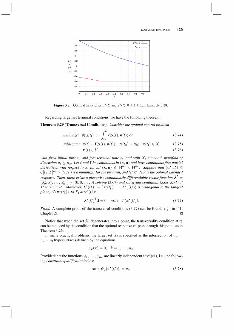
MAXIMUM PRINCIPLES 139
-1
-0.8
-0.6
-0.4
-0.2
0
0.2
0.4
0.6
0.8
1
0 0.1 0.2 0.3 0.4 0.5 0.6 0.7 0.8 0.9 1
PSfrag replacements
t
u(t
),x(t
)
x?(t)
u?(t)
Figure 3.8. Optimal trajectories u?(t) and x?(t), 0 ≤ t ≤ 1, in Example 3.28.
Regarding target set terminal conditions, we have the following theorem:
Theorem 3.29 (Transversal Conditions). Consider the optimal control problem
minimize: J(u, tf) :=
∫ tf
t0
`(x(t),u(t)) dt (3.74)
subject to: x(t) = f(x(t),u(t)); x(t0) = x0; x(tf) ∈ Xf (3.75)u(t) ∈ U, (3.76)
with fixed initial time t0 and free terminal time tf, and with Xf a smooth manifold ofdimension nf ≤ nx. Let ` and f be continuous in (x,u) and have continuous first partialderivatives with respect to x, for all (x,u) ∈ IRnx × IRnu . Suppose that (u?, t?f ) ∈C [t0, T ]nu × [t0, T ) is a minimizer for the problem, and let x? denote the optimal extendedresponse. Then, there exists a piecewise continuously differentiable vector function λ
?=
(λ?0, λ?1, . . . , λ
?nx
) 6= (0, 0, . . . , 0) solving (3.67) and satisfying conditions (3.68–3.71) ofTheorem 3.26. Moreover, λ?(t?f ) := (λ?1(t
?f ), . . . , λ?nx(t
?f )) is orthogonal to the tangent
plane, T (x?(t?f )), to Xf at x?(t?f ):
λ?(t?f )Td = 0, ∀d ∈ T (x?(t?f )). (3.77)
Proof. A complete proof of the transversal conditions (3.77) can be found, e.g., in [41,Chapter 2].
Notice that when the set Xf degenerates into a point, the transversality condition at t?fcan be replaced by the condition that the optimal response x? pass through this point, as inTheorem 3.26.
In many practical problems, the target set Xf is specified as the intersection of nψ =nx − nf hypersurfaces defined by the equations
ψk(x) = 0, k = 1, . . . , nψ.
Provided that the functionsψ1, . . . , ψnψ are linearly independent at x?(t?f ), i.e., the follow-ing constraint qualification holds:
rank[ψx(x?(t?f ))] = nψ, (3.78)
140 OPTIMAL CONTROL
the tangent set T (x?(t?f )) is such that
T (x?(t?f )) = d ∈ IRnx : ψx(x?(t?f )) d = 0,
(see, e.g., Lemma 1.48, p. 23). For the transversal condition (3.77) to be satisfied, it is thusnecessary that λ?(t?f ) be in the subspace spanned by the row vectors of ψx(x?(t?f )); inother words, there must exist a vector ν of Lagrange multipliers such that
λ?(t?f ) = νTψx(x?(t?f )),
hence yielding the same terminal adjoint condition as in Theorem 3.18.
We now turn to the extension of the PMP for non-autonomous problems. We shallconsider the optimal control problem in the same form as in (3.64–3.66), but for the casein which ` and f depend explicitly on time (the control regionU is assumed independent oftime). Thus, the system equations and the cost functional take the form
x(t) = f(t,x(t),u(t)) (3.79)
J(u, tf) :=
∫ tf
t0
`(t,x(t),u(t)) dt.
In order to solve this problem, we shall introduce yet another auxiliary variable, xnx+1,defined by
xnx+1(t) = 1; xnx+1(t0) = t0.
It is obvious that xnx+1(t) = t, t0 ≤ t ≤ tf. Therefore, we get the (nx + 1)-dimensionalsystem
x(t) = f(xnx+1(t),x(t),u(t))
xnx+1(t) = 1.
Next, we apply the autonomous version of the PMP with transversal conditions (Theo-rem 3.29) to find necessary conditions of optimality, in terms of the (nx + 2)-dimensionalvector (c,xT, xnx+1), where
c = `(xnx+1(t),x(t),u(t)); c(t0) = 0.
Using the same notations as in 3.5.1 for the extended response, xT := (c,xT), and
the extended system, fT
:= (`, fT), the equations giving the (nx + 2) adjoint variables
(λT, λnx+1) := (λ0, λ1, . . . , λnx , λnx+1) read
λ0(t) = 0
λi(t) = − λ(t)Tfxi(xnx+1,x,u), i = 1, . . . , nx
λnx+1(t) = − λ(t)Tf t(xnx+1,x,u).
Moreover, the transversal condition at tf requires that Xf (which is parallel to the xnx+1
axis) be orthogonal to the vector (λ1, . . . , λnx , λnx+1). But since Xf is parallel to thexnx+1 axis, it follows that
λnx+1(tf) = 0.

MAXIMUM PRINCIPLES 141
Overall, a version of the PMP for non-autonomous system is as follows:
Theorem 3.30 (Pontryagin Maximum Principle for Non-Autonomous Systems). Con-sider the optimal control problem
minimize: J(u, tf) :=
∫ tf
t0
`(t,x(t),u(t)) dt (3.80)
subject to: x(t) = f(t,x(t),u(t)); x(t0) = x0; x(tf) = xf (3.81)u(t) ∈ U, (3.82)
with fixed initial time t0 and free terminal time tf. Let ` and f be continuous in(t,x,u) and have continuous first partial derivatives with respect to (t,x), for all(t,x,u) ∈ [t0, T ] × IRnx × IRnu . Suppose that (u?, t?f ) ∈ C [t0, T ]nu × [t0, T ) isa minimizer for the problem, and let x? denote the optimal extended response. Then,there exists a (nx + 1)-dimensional, piecewise continuously differentiable vector functionλ?
= (λ?0, λ?1, . . . , λ
?nx
) 6= (0, 0, . . . , 0) such that
˙λ?
(t) =−Hx(t,x?(t),u?(t), λ?(t)), (3.83)
with H(t,x,u, λ) := λTf(t,x,u), and:
(i) the functionH(x?(t),v, λ?(t)) attains its minimum on U at v = u?(t):
H(t,x?(t),v, λ?(t)) ≥ H(t,x?(t),u?(t), λ
?(t)), ∀v ∈ U, (3.84)
for every t0 ≤ t ≤ t?f ;
(ii) the following relations
λ?0(t) = const. ≥ 0 (3.85)
H(t,x?(t),u?(t), λ?(t)) = λ
?(t)
Tf t(t,x
?(t),u?(t)), (3.86)
are satisfied at any t ∈ [t0, t?f ]. Moreover, in the case wherein the final time is
unspecified, t?f is determined from the transversal condition
H(t?f ,x?(t?f ),u?(t?f ), λ
?(t?f )) = 0. (3.87)
3.5.3 Application: Linear Time-Optimal Problems
An interesting application of the PMP is in the special case of a linear time-invariant systemand a linear cost functional,
minimize: J(u, tf) :=
∫ tf
t0
[aTu(t) + bTx(t) + c] dt (3.88)
subject to: x(t) = Fx(t) + Gu(t); x(t0) = x0; x(tf) = xf (3.89)u(t) ∈ U. (3.90)
with fixed initial time t0 and free terminal time tf. In the case where the control regionU isunbounded, no minimum exists, in general, for such problems; this is because the control
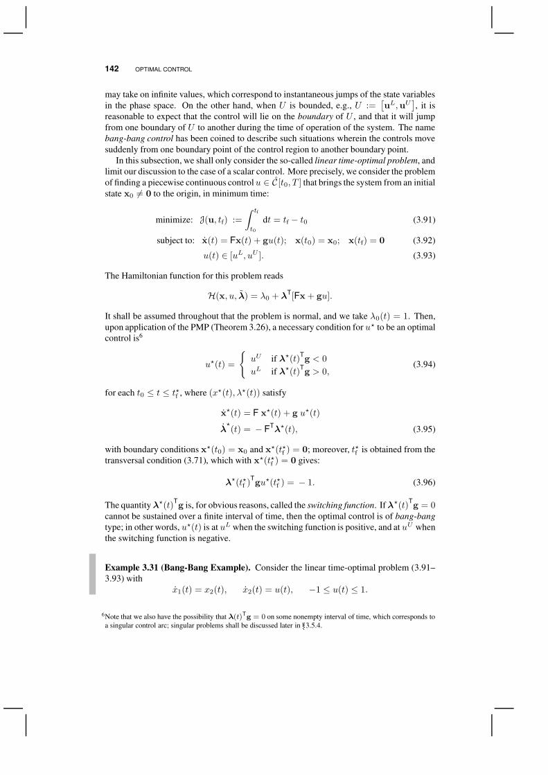
142 OPTIMAL CONTROL
may take on infinite values, which correspond to instantaneous jumps of the state variablesin the phase space. On the other hand, when U is bounded, e.g., U :=
[
uL,uU]
, it isreasonable to expect that the control will lie on the boundary of U , and that it will jumpfrom one boundary of U to another during the time of operation of the system. The namebang-bang control has been coined to describe such situations wherein the controls movesuddenly from one boundary point of the control region to another boundary point.
In this subsection, we shall only consider the so-called linear time-optimal problem, andlimit our discussion to the case of a scalar control. More precisely, we consider the problemof finding a piecewise continuous controlu ∈ C [t0, T ] that brings the system from an initialstate x0 6= 0 to the origin, in minimum time:
minimize: J(u, tf) :=
∫ tf
t0
dt = tf − t0 (3.91)
subject to: x(t) = Fx(t) + gu(t); x(t0) = x0; x(tf) = 0 (3.92)
u(t) ∈ [uL, uU ]. (3.93)
The Hamiltonian function for this problem reads
H(x, u, λ) = λ0 + λT[Fx + gu].
It shall be assumed throughout that the problem is normal, and we take λ0(t) = 1. Then,upon application of the PMP (Theorem 3.26), a necessary condition for u? to be an optimalcontrol is6
u?(t) =
uU if λ?(t)Tg < 0
uL if λ?(t)Tg > 0,
(3.94)
for each t0 ≤ t ≤ t?f , where (x?(t), λ?(t)) satisfy
x?(t) = F x?(t) + g u?(t)
λ?(t) = − FT
λ?(t), (3.95)
with boundary conditions x?(t0) = x0 and x?(t?f ) = 0; moreover, t?f is obtained from thetransversal condition (3.71), which with x?(t?f ) = 0 gives:
λ?(t?f )Tgu?(t?f ) = − 1. (3.96)
The quantityλ?(t)Tg is, for obvious reasons, called the switching function. Ifλ?(t)T
g = 0cannot be sustained over a finite interval of time, then the optimal control is of bang-bangtype; in other words, u?(t) is at uL when the switching function is positive, and at uU whenthe switching function is negative.
Example 3.31 (Bang-Bang Example). Consider the linear time-optimal problem (3.91–3.93) with
x1(t) = x2(t), x2(t) = u(t), −1 ≤ u(t) ≤ 1.
6Note that we also have the possibility that λ(t)Tg = 0 on some nonempty interval of time, which corresponds to
a singular control arc; singular problems shall be discussed later in 3.5.4.

MAXIMUM PRINCIPLES 143
For this simple system, an optimal control u? must satisfy
u?(t) =
1 if λ?2(t) < 0−1 if λ?2(t) > 0.
The adjoint variables λ? verify the differential equations (3.95),
λ?1(t) = 0
λ?2(t) = − λ?1(t),
which are readily solved as
λ1?(t) = A1
λ2?(t) = −A1t+A2,
where A1 and A2 are constants of integration. That is, the switching function λ?(t)Tg =
−A1t + A2 is a linear function of time, and it follows that every optimal control u?(t),t0 ≤ t ≤ t?f , is a piecewise constant function which takes on the values±1, and has at mosttwo intervals on which it is constant.
For the time interval on which u?(t) = 1, we have
x?2(t) = t+K1, x?1(t) =t2
2+K2t+K1 =
1
2(t+K2)
2 +
(
K1 −K2
2
2
)
,
(where K1 and K2 are constants of integration), from which we get
x?1(t) =1
2[x?2(t)]
2 +K, (3.97)
withK = K1− 12K
22 . Thus, the portion of the optimal response for which u(t) = 1
is an arc of the parabola (3.97), along which the phase points move upwards (sincex2 = 1 > 0).
analogously, for the time interval on which u?(t) = −1, we have
x?2(t) = −t+K ′1, x?1(t) =
t2
2+K ′
2t+K′1 = −1
2(−t+K ′
2)2 +
(
K ′1 +
K ′22
2
)
,
from which we obtain
x?1(t) = − 1
2[x?2(t)]
2 +K ′. (3.98)
thus, the portion of the optimal response for whichu(t) = −1 is an arc of the parabola(3.98), along which the phase points move downwards (since x2 = −1 < 0).
Observe that if u? is initially equal to 1, and to−1 afterwards, the response consists of twoadjoining parabolic arcs, and the second arc lies on that parabola defined by (3.98) whichpasses through the origin:
x?1(t) = − 1
2[x?2(t)]
2. (3.99)

144 OPTIMAL CONTROL
Likewise, if u? = −1 first, and u? = 1 afterwards, the second arc lies on that paraboladefined by (3.97) which passes through the origin:
x?1(t) =1
2[x?2(t)]
2. (3.100)
The switching curve is therefore made up of the parabolas (3.99) (for x2 > 0) and (3.100)(for x2 < 0). By inspection, it is apparent that (i) u? = −1 above the switching curve, and(ii) u? = 1 below the switching curve. Overall, the optimal feedback law for the problemmay thus be written as:
u?(t) =
1 if [x?2]2 signx2 < −2x?1 or [x?2]
2 signx2 = −2x?1, x?1 > 0
−1 if [x?2]2 signx2 > −2x?1 or [x?2]
2 signx2 = −2x?1, x?1 < 0.
The switching curve is illustrated in Fig. 3.9. below, along with typical optimal responsesobtained for different initial conditions.
-1.5
-1
-0.5
0
0.5
1
1.5
-1 -0.5 0 0.5 1
PSfrag replacements
x1
x2
x−0
x+0
u ?= +1
u ?= −1
u ?= +1
u ?= −1
switchingcurve
Figure 3.9. Switching curve and typical optimal responses for Example 3.31 — Red line: switchingcurve; blue line: typical path.
3.5.4 Singular Optimal Control Problems
In all the optimal control problems considered so far, the values u?(t) of candidate optimalcontrols could be explicitly determined by a minimum condition such as
H(t,x?(t),v, λ?(t)) ≥ H(t,x?(t),u?(t), λ
?(t)), ∀v ∈ U, (3.101)
at each time instant t ∈ [t0, tf]. However, it may happen for some problems that u?(t)cannot be directly determined by the foregoing condition.

MAXIMUM PRINCIPLES 145
To illustrate this situation, consider the following (scalar) optimal control problem:
minimize: J(u) :=
∫ tf
t0
`0(t,x(t)) + u(t) `1(t,x(t)) dt
subject to: x(t) = f0(t,x(t)) + u(t) f1(t,x(t)); x(t0) = x0; x(tf) = xf
u(t) ∈ U := [uL, uU ],
for u ∈ C [t0, tf], with fixed initial time t0 and final time tf. Since the Hamiltonian functionis affine in the control u (i.e., contains u in at most the first power), we have
H(t,x, u, λ) = H0(t,x, λ) + u(t) H1(t,x, λ),
whereH0 := λ0`
0 + λTf 0, and H1 := λ1`1 + λTf1.
To minimize the Hamiltonian function at a given t ∈ [t0, tf], one has to take u?(t) = uU ifH1(t,x?(t), λ
?(t)) > 0, and u?(t) = uL if H1(t,x?(t), λ
?(t)) < 0. We then have either
one of two situations:
(i) If the term H1(t,x?(t), λ?(t)) vanishes only at isolated times, then the control u
switches from uL to uU or vice versa each timeH1(t,x?(t), λ?(t)) crosses zero; the
control is said to be bang-bang. An illustration of this behavior was given earlier inExample 3.31.
(ii) On the other hand, if H1(t,x?(t), λ?(t)) = 0 can be sustained over some finite
interval (θ1, θ2) ⊂ [t0, tf], then any value ofu ∈ [uL, uU ] trivially meets the minimumcondition (3.101). In other words, the control does not affect the Hamiltonian functionon (θ1, θ2), and we have a singular arc.
For more general scalar optimal control problems of the form (3.80–3.82), singular arcsare obtained when the stationarity condition
Hu(t,x?(t), u, λ?(t)) = 0,
is trivially satisfied by any admissible control on some nonempty subinterval (θ1, θ2) ⊂[t0, tf], i.e., the matrix Huu is singular. In the case of a vector control problem, the subse-quent developments apply readily to each component uk(t), k = 1, . . . , nu, of u(t).
The following idea is used to determine the value of an optimal control along a singulararc. SinceHu = 0 for all t ∈ (θ1, θ2), its successive time derivatives dq
dtqHu, q = 1, 2, . . .,must also vanish on (θ1, θ2). In particular, we may find a smallest positive integer q suchthat
dq
dtqHu(t,x?(t), ·, λ
?(t)) = 0
∂
∂u
[
dq
dtqHu(t,x?(t), ·, λ?(t))
]
6= 0.
Note that if such a smallest integer q exists, it must be even (see, e.g., [29] for a proof).Then, the nonnegative integer p such that q = 2p is called the order of the singular arc. Notealso that singular arcs are not possible at all points of the (x, λ)-space. Along a singular
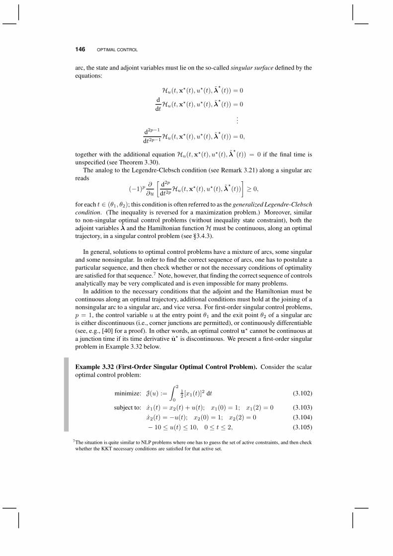
146 OPTIMAL CONTROL
arc, the state and adjoint variables must lie on the so-called singular surface defined by theequations:
Hu(t,x?(t), u?(t), λ?(t)) = 0
ddtHu(t,x?(t), u?(t), λ
?(t)) = 0
...
d2p−1
dt2p−1Hu(t,x?(t), u?(t), λ
?(t)) = 0,
together with the additional equation Hu(t,x?(t), u?(t), λ?(t)) = 0 if the final time is
unspecified (see Theorem 3.30).The analog to the Legendre-Clebsch condition (see Remark 3.21) along a singular arc
reads
(−1)p∂
∂u
[
d2p
dt2pHu(t,x?(t), u?(t), λ
?(t))
]
≥ 0,
for each t ∈ (θ1, θ2); this condition is often referred to as the generalized Legendre-Clebschcondition. (The inequality is reversed for a maximization problem.) Moreover, similarto non-singular optimal control problems (without inequality state constraint), both theadjoint variables λ and the Hamiltonian functionH must be continuous, along an optimaltrajectory, in a singular control problem (see 3.4.3).
In general, solutions to optimal control problems have a mixture of arcs, some singularand some nonsingular. In order to find the correct sequence of arcs, one has to postulate aparticular sequence, and then check whether or not the necessary conditions of optimalityare satisfied for that sequence.7 Note, however, that finding the correct sequence of controlsanalytically may be very complicated and is even impossible for many problems.
In addition to the necessary conditions that the adjoint and the Hamiltonian must becontinuous along an optimal trajectory, additional conditions must hold at the joining of anonsingular arc to a singular arc, and vice versa. For first-order singular control problems,p = 1, the control variable u at the entry point θ1 and the exit point θ2 of a singular arcis either discontinuous (i.e., corner junctions are permitted), or continuously differentiable(see, e.g., [40] for a proof). In other words, an optimal control u? cannot be continuous ata junction time if its time derivative u? is discontinuous. We present a first-order singularproblem in Example 3.32 below.
Example 3.32 (First-Order Singular Optimal Control Problem). Consider the scalaroptimal control problem:
minimize: J(u) :=
∫ 2
0
12 [x1(t)]
2 dt (3.102)
subject to: x1(t) = x2(t) + u(t); x1(0) = 1; x1(2) = 0 (3.103)x2(t) = −u(t); x2(0) = 1; x2(2) = 0 (3.104)− 10 ≤ u(t) ≤ 10, 0 ≤ t ≤ 2, (3.105)
7The situation is quite similar to NLP problems where one has to guess the set of active constraints, and then checkwhether the KKT necessary conditions are satisfied for that active set.
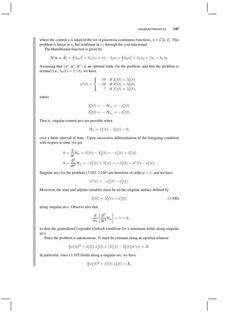
MAXIMUM PRINCIPLES 147
where the control u is taken in the set of piecewise continuous functions, u ∈ C [0, 2]. Thisproblem is linear in u, but nonlinear in x1 through the cost functional.
The Hamiltonian function is given by
H(x, u, λ) = 12λ0x
21 + λ1(x2 + u)− λ2u = 1
2λ0x21 + λ1x2 + (λ1 − λ2)u.
Assuming that (u?,x?,λ?) is an optimal triple for the problem, and that the problem isnormal (i.e., λ0(t) = 1, ∀t), we have
u?(t) =
10 if λ?1(t) < λ?2(t)−10 if λ?1(t) > λ?2(t)
? if λ?1(t) = λ?2(t),
where
λ?1(t) = −Hx1= −x?1(t)
λ?2(t) = −Hx2= −λ?1(t).
That is, singular control arcs are possible when
Hu = λ?1(t)− λ?2(t) = 0,
over a finite interval of time. Upon successive differentiation of the foregoing conditionwith respect to time, we get
0 =ddtHu = λ?1(t)− λ?2(t) = −x?1(t) + λ?1(t)
0 =d2
dt2Hu = −x?1(t) + λ?1(t) = −x?2(t)− u?(t)− x?1(t).
Singular arcs for the problem (3.102–3.105) are therefore of order p = 1, and we have
u?(t) = −x?1(t)− x?2(t).
Moreover, the state and adjoint variables must lie on the singular surface defined by
λ?1(t) = λ?2(t) = x?1(t), (3.106)
along singular arcs. Observe also that
− ∂
∂u
[
d2
dt2Hu]
= 1 > 0,
so that the generalized Legendre-Clebsch condition for a minimum holds along singulararcs.
Since the problem is autonomous,H must be constant along an optimal solution:
12x
?1(t)
2 + λ?1(t) x?2(t) + [λ?1(t)− λ?2(t)]u?(t) = K.
In particular, since (3.105) holds along a singular arc, we have
12x
?1(t)
2 + x?1(t) x?2(t) = K,

148 OPTIMAL CONTROL
which gives a 1-parameter family of hyperbolas in the (x1, x2)-space.Upon application of a numerical optimization procedure, it is found that an optimal
control for the problem (3.102–3.105) consists of 3 arcs:
1. u?(t) = 10, 0 ≤ t ≤ t?1;
2. u?(t) = −x?1(t)− x?2(t), t?1 ≤ t ≤ t?2;
3. u?(t) = −10, t?2 ≤ t ≤ 2.
with the following approximate values for the intermediate times: t?1 ≈ 0.299, and t?2 ≈1.927. This optimal control, together with the optimal response of the system is representedin Fig. 3.10. below. Note that this control is discontinuous at the junction points betweensingular and a non-singular arcs. Hence, all the necessary conditions of optimality aresatisfied.
-10
-5
0
5
10
0 0.5 1 1.5 2
PSfrag replacements
t
u?(t
)
x?1(t)x?2(t)x0
t?1 ≈ 0.299
t?2 ≈ 1.927
u? = −10u? = +10
u? = −x?1 − x?2
-2.5
-2
-1.5
-1
-0.5
0
0.5
1
1.5
0 0.5 1 1.5 2 2.5 3 3.5 4
PSfrag replacementst
u?(t)
x?1(t)
x? 2(t
)
x0
t?1 ≈ 0.299t?2 ≈ 1.927
u? = −10u? = +10
u? = −x?1 − x?2
Figure 3.10. Optimal control and response for Example 3.31 – left plot: optimal control vs. time;right plot: optimal response in the phase space.

MAXIMUM PRINCIPLES 149
The junction phenomenon for higher-order singular control problems is a notoriouslyhard problem, and is still the topic of a great deal of research. In particular, the controlsnear high-order singular surface may exhibit a chattering behavior, i.e, the control has aninfinite number of discontinuities in a finite time interval (see, e.g., [58] for more details).
At first sight, one may reasonably expect that a “nice” optimal control problem shouldhave a “nice” solution, and that most if not all reasonable optimal control problems havesmooth or piecewise smooth solutions. In 1961, A. T. Fuller [21] put this myth to rest byexhibiting a very simple optimal control problem whose solution chatters.
3.5.5 Optimal Control Problems with Mixed Control-State InequalityConstraints
Optimal control problems with state inequality constraints arise frequently in practicalapplications. These problems are notoriously hard to solve, and even the theory is notunambiguous, since there exist various forms of the necessary conditions of optimality. Werefer the reader to [25] for a recent survey of the various forms of the maximum principlefor problems with state inequality constraints. In this subsection, we shall consider optimalcontrol problems with mixed control-state inequality constraints only. Problems with mixedcontrol-state inequality constraints shall be considered later on in 3.5.6.
Consider the problem to find a piecewise continuous control u? ∈ C [t0, T ]nu , withassociated response x? ∈ C1[t0, T ]nx , and a terminal time t?f ∈ [t0, T ], such that thefollowing constraints are satisfied and the cost functional takes on its minimum value:
minimize: J(u, tf) :=
∫ tf
t0
`(t,x(t),u(t)) dt (3.107)
subject to: x(t) = f(t,x(t),u(t)); x(t0) = x0; x(tf) = xf (3.108)gk(t,x(t),u(t)) ≤ 0, k = 1, . . . , ng. (3.109)
In what follows, we shall always assume that the components of g depend explicitly on thecontrol u, and the following constraint qualification holds:
rank[
gu diag (g)]
= ng , (3.110)
along (t,x?(t),u?(t)), t0 ≤ t ≤ t?f . In other words, the gradients with respect to u of allthe active constraints g ≤ 0 must be linearly independent.
A possible way of tackling optimal control problems with mixed inequality constraintsof the form (3.109), is to form a Lagrangian function L by adjoining g to the HamiltonianfunctionH with a Lagrange multiplier vector function µ,
L(t,x,u,λ,µ) := H(t,x,u,λ) + µTg(t,x,u), (3.111)
where
H(t,x,u,λ) := λTf (t,x,u) = λ0`(t,x,u) + λTf(t,x,u). (3.112)
The corresponding necessary conditions of optimality are stated in the following theorem:
Theorem 3.33 (Maximum Principle with Mixed Inequality Constraints). Consider theoptimal control problem (3.107–3.109), with fixed initial time t0 and free terminal time tf,and where `, f , and g are continuous and have continuous first partial derivatives with

150 OPTIMAL CONTROL
respect to (t,x,u) on [t0, T ]× IRnx × IRnu . Suppose that (u?, t?f ) ∈ C [t0, T ]nu × [t0, T )is a minimizer for the problem, and let x? denote the optimal (extended) response. If theconstraint qualification (3.110) holds, then there exist a (nx + 1)-dimensional piecewisecontinuously differentiable vector function λ
?(·) = (λ?0(·),λ?(·)), and a ng-dimensional
piecewise continuous vector function µ?(·), such that (λ?(t),µ?(t)) 6= 0 for every t ∈
[t0, t?f ], and:
(i) the functionH(x?(t),v, λ?(t)) attains its minimum onU(x?(t), t) at v = u?(t), for
every t ∈ [t0, t?f ],
H(t,x?(t),v, λ?(t)) ≥ H(t,x?(t),u?(t), λ
?(t)), ∀v ∈ U(x?(t), t), (3.113)
where U(x, t) := u ∈ IRnu : g(t,x,u) ≤ 0;
(ii) the quadruple (u?,x?, λ?,µ?) verifies the equations
˙x?(t) = Lλ(t,x?(t),u?(t), λ
?(t),µ?(t)) (3.114)
˙λ?
(t) = −Lx(t,x?(t),u?(t), λ?(t),µ?(t)) (3.115)
0 = Lu(t,x?(t),u?(t), λ?(t),µ?(t)), (3.116)
at each instant t of continuity of u?;
(iii) the vector functionµ? is continuous at each instant t of continuity of u?, and satisfies
µ?k(t) gk(t,x?(t),u?(t)) = 0, µ?k(t) ≥ 0, (3.117)
for each k = 1, . . . , ng;
(iv) the relations
λ?0(t) = const. ≥ 0 (3.118)
H(t,x?(t),u?(t), λ?(t)) = −
∫ t?f
t
Lt(τ,x?(τ),u?(τ), λ?(τ),µ?(τ)) dτ,
(3.119)
are satisfied at any t ∈ [t0, t?f ], and, in particular,H(t?f ,x
?(t?f ),u?(t?f ), λ
?(t?f )) = 0.
Proof. A proof of the theorem can be found, e.g., in [48] or [23]. See also [25] for discus-sions.
Similar to problems with simple control constraints of the form u(t) ∈ U , t0 ≤ t ≤ tf,solutions to optimal control problems with mixed inequality constraints consist of severalconstrained and unconstrained arcs, which must be pieced together in order to satisfy allthe necessary conditions. At the junction points between constrained and unconstrainedarcs, the optimal control may or may not be continuous; in the latter case, we get a cornerpoint.8 In particular, the conditions that must hold at any corner point θ ∈ [t0, t
?f ] are
x?(θ−) = x?(θ+) (3.120)
λ?(θ−) = λ
?(θ+) (3.121)
H(θ−,x?(θ),u?(θ−), λ?(θ)) =H(θ+,x?(θ),u?(θ+), λ
?(θ)), (3.122)
8As noted in 3.4.3, corners may occur at any point of an optimal trajectory, although they are more likely to occurat junction points rather than at the middle of unconstrained arcs.

MAXIMUM PRINCIPLES 151
where θ− and θ+ denote the time just before and just after the corner, respectively; z(θ−)and z(θ+) denote the left and right limit values of a quantity z at θ, respectively. Sinceeach component of Lu is also continuous across θ, it follows that µ(t) is continuous ifu?(t) is itself continuous across θ. Unfortunately, there seems to be no a priori method fordetermining the existence of corners.
Remark 3.34 (Extension to General State Terminal Constraints). The Maximum Prin-ciple in Theorem 3.33 can be extended to the case where general terminal constraints arespecified on the state variables (in lieu of the terminal state condition x(tf) = xf) as
ψk(tf,x(tf)) = 0, k = 1, . . . , nψ. (3.123)κk(tf,x(tf)) ≤ 0, k = 1, . . . , nκ, (3.124)
and a terminal term is added to the cost functional (3.107) as
J(u, tf) :=
∫ tf
t0
`(t,x(t),u(t)) dt+ φ(tf,x(tf)), (3.125)
where φ, ψ, and κ are continuous and have continuous first partial derivatives with respectto (t,x), for all (t,x) ∈ [t0, T ]× IRnx . Suppose that the terminal constraints (3.123,3.124)satisfy the constraint qualification
rank
[
ψx 0κx diag (κ)
]
= nψ + nκ, (3.126)
at (t?f ,x?(t?f )). Then, in addition to the necessary conditions of optimality given in Theo-
rem 3.33, there exist Lagrange multiplier vectors ν? ∈ IRnψ and ζ? ∈ IRnκ such that thefollowing transversal conditions hold:
λ?(t?f ) = Φx(t?f ,x?(t?f )) (3.127)
H(t?f ,x?(t?f ),u
?(t?f ),λ?(t?f )) + Φt(t
?f ,x
?(t?f )) = 0, (3.128)
where Φ := λ?0φ+ ν?Tψ + ζ?Tκ. Moreover,
ψk(t?f ,x
?(t?f )) = 0, (3.129)
for each k = 1, . . . , nψ, and
ζ?k κk(t?f ,x
?(t?f )) = 0, ζ?k ≥ 0, (3.130)
for each k = 1, . . . , nκ.
In practice, applying Theorem 3.33 (and Remark 3.34) requires that an assumptionbe made a priori on the sequence of (unconstrained and constrained) arcs in the optimalsolution, as well as on the set of active (inequality) terminal constraints. Then, based onthe postulated structure of the optimal solution, one shall check whether a pair (u(·),x(·)),along with vector functions λ(·), µ(·), and Lagrange multiplier vectors ν?, ζ?, can befound such that all of the necessary conditions of optimality are satisfied. If this is the case,then the corresponding control is a candidate optimal control for the problem; otherwise,one needs to investigate alternative solution structures, i.e., postulate different sequencesof arcs and/or sets of active terminal constraints. An illustration of these considerations ingiven in Example 3.35 hereafter.
152 OPTIMAL CONTROL
Example 3.35 (Optimal Control Problem with Mixed Inequality Constraints). Con-sider the scalar optimal control problem:
minimize: J(u) :=
∫ 1
0
u(t) dt (3.131)
subject to: x(t) = −u(t); x(0) = −1 (3.132)u(t) ≤ 0, x(t)− u(t) ≤ 0, 0 ≤ t ≤ 1, (3.133)
where the control u is taken in the set of piecewise continuous functions, u ∈ C [0, 1].Observe that both path constraints are of mixed type, and can be rewritten as
x(t) ≤ u(t) ≤ 0, 0 ≤ t ≤ 1. (3.134)
The objective being to minimize the integral of u(t), and since u(t) is lower bounded bythe state x(t) via (3.134), a rather natural guess for the optimal solution is to consider thatthe mixed state constraint x(t)−u(t) ≤ 0 is active for each 0 ≤ t ≤ 1. We shall now checkwhether the necessary conditions of optimality in Theorem 3.33 can be satisfied under thischoice.
Let us suppose first that the problem (3.131–3.133) is not abnormal, and take λ0(t) =1 throughout. That is, the Hamiltonian function for the problem reads
H(x, u, λ) = u(1− λ),
and the Lagrangian function, obtained by adjoining the mixed inequality constraints,reads
L(x, u, λ,µ) = H(x, u, λ) + µ1(x− u) + µ2u = (1− λ− µ1 + µ2)u+ µ1x.
The mixed state constraint x(t)−u(t) ≤ 0 being active for each 0 ≤ t ≤ 1, we have
u?(t) = x?(t),
and, from (3.132),x?(t) = −e−t, 0 ≤ t ≤ 1.
x?(t) and, hence, u?(t) are thus negative at any time, and from the complementarityslackness condition (3.117) we get
µ?2(t) = 0, 0 ≤ t ≤ 1.
In turn, the stationarity condition (3.116) yields
0 = 1− λ?(t)− µ?1(t) + µ?2(t) = 1− λ?(t)− µ?1(t),
from which we getµ?1(t) = 1− λ?(t), 0 ≤ t ≤ 1.
From (3.115), the differential equation giving the adjoint variable λ? is
λ?(t) = −µ?1(t) = λ?(t)− 1,

MAXIMUM PRINCIPLES 153
and the terminal state being unspecified, from (3.127), we get
λ?(1) = 0.
Therefore,
λ?(t) = 1− et−1 < 1, 0 ≤ t ≤ 1,
and,
µ?1(t) = et−1 > 0, 0 ≤ t ≤ 1,
hence satisfying the dual condition (3.117).
At this point, the condition (3.119)imposing that the Hamiltonian function be constantalong (u?, x?, λ?) is readily verified,
H(x?(t), u?(t), λ?(t)) = u?(t)(1− λ?(t)) = −e−1, 0 ≤ t ≤ 1.
Finally, the minimum condition (3.113),
u?(t) =
0 if λ?(t) > 1x?(t) if λ?(t) < 1,
is satisfied by the control u?(t) = x?(t), since λ?(t) < 1 at each 0 ≤ t ≤ 1.
Overall, we have checked that all the necessary conditions of optimality are satisfied pro-vided that the mixed state constraint x(t) − u(t) ≤ 0 is active at any time. Therefore,u?(t) = x?(t) = −e−t, 0 ≤ t ≤ 1, is a candidate optimal control for the problem (3.131–3.133).
3.5.6 Optimal Control Problems with Pure State Inequality Constraints
Besides mixed state inequality constraints, it is common to require that one or several statevariables remain nonnegative during the system operation, e.g.,
xi(t) ≥ 0, t0 ≤ t ≤ tf,
for i ∈ 1, . . . , nx. More generally, optimal control problems may have so-called purestate inequality constraints of the form
hk(t,x(t)) ≤ 0, k = 1, . . . , nh.
Pure state constraints are, in principle, more difficult to deal with than mixed control-stateconstraints, since h does not explicitly depend on u, and x can be controlled only indirectlyvia propagation through the state equations. It is therefore convenient to differentiate hwith respect to t as many times as required until it contains a control variable. For the jth
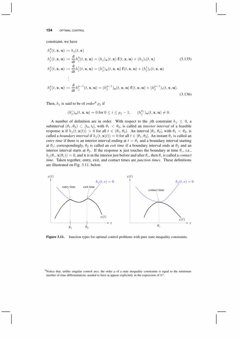
154 OPTIMAL CONTROL
constraint, we have
h0j (t,x,u) := hj(t,x)
h1j (t,x,u) :=
ddth0j (t,x,u) = (hj)x(t,x) f(t,x,u) + (hj)t(t,x) (3.135)
h2j (t,x,u) :=
ddth1j (t,x,u) = (h1
j )x(t,x,u) f(t,x,u) + (h1j )t(t,x,u)
...
hpj (t,x,u) :=ddthp−1j (t,x,u) = (hp−1
j )x(t,x,u) f (t,x,u) + (hp−1j )t(t,x,u).
(3.136)
Then, hj is said to be of order9 pj if
(hij)u(t,x,u) = 0 for 0 ≤ i ≤ pj − 1, (hpjj )u(t,x,u) 6= 0.
A number of definition are in order. With respect to the jth constraint hj ≤ 0, asubinterval (θ1, θ2) ⊂ [t0, tf], with θ1 < θ2, is called an interior interval of a feasibleresponse x if hj(t,x(t)) > 0 for all t ∈ (θ1, θ2). An interval [θ1, θ2], with θ1 < θ2, iscalled a boundary interval if hj(t,x(t)) = 0 for all t ∈ [θ1, θ2]. An instant θ1 is called anentry time if there is an interior interval ending at t = θ1 and a boundary interval startingat θ1; correspondingly, θ2 is called an exit time if a boundary interval ends at θ2 and aninterior interval starts at θ2. If the response x just touches the boundary at time θc, i.e.,hj(θc,x(θc)) = 0, and x is in the interior just before and after θc, then θc is called a contacttime. Taken together, entry, exit, and contact times are junction times. These definitionsare illustrated on Fig. 3.11. below.
PSfrag replacements
t t
x(t)
x(t) x(t)
x(t)
hj(t, x) = 0 hj(t, x) = 0
entry time exit timecontact time
θ1 θ2 θc
Figure 3.11. Junction types for optimal control problems with pure state inequality constraints.
9Notice that, unlike singular control arcs, the order p of a state inequality constraints is equal to the minimumnumber of time differentiations needed to have u appear explicitely in the expression of hp.
MAXIMUM PRINCIPLES 155
We begin with the case of first-order state inequality constraints, pj = 1, i = 1, . . . , nh.Let (u?,x?) be an optimal pair for the problem
minimize: J(u, tf) :=
∫ tf
t0
`(t,x(t),u(t)) dt (3.137)
subject to: x(t) = f(t,x(t),u(t)); x(t0) = x0; x(tf) = xf (3.138)hk(t,x(t)) ≤ 0, k = 1, . . . , nh. (3.139)
We shall always assume that the constraint qualification
rank[
h1u diag (h)
]
= nh, (3.140)
holds at each (t,x?(t),u?(t)); i.e., the gradients of h1j with respect to u of the active
constraints hj = 0, j ∈ 1, . . . , nh, must be linearly independent along an optimaltrajectory.
Suppose that [θ1, θ2] is a boundary interval for the jth constraint. In order to preventhj from being violated, we must have that h1
j (t,x?(t),u?(t)) ≤ 0 for each t ∈ [θ1, θ2].
Hence, one can formally impose the constraint
h1j (t,x
?(t),u?(t)) ≤ 0 whenever hj(t,x?(t)) = 0.
A convenient way of associating a multiplier functionηj(·) to the former condition constraintis by imposing the complementarity slackness condition ηj(t)hj(t,x
?(t)) = 0, whichmakes ηj(t) = 0 each time hj(t,x?(t)) < 0. This also motivates the following definitionof the Lagrangian function:
L1(t,x,u,λ,η) := H(t,x,u,λ) + ηTh1(t,x,u). (3.141)
Since the constraints are adjoined indirectly to form the Lagrangian (i.e., they are adjoinedvia their first time derivative), this approach is called the indirect adjoining approach; itwas first suggested by Pontryagin [41].10
At the entry time θ1 of a boundary interval for the jth constraint, it is necessary to requirethat the interior-point constraint
hj(θ1,x?(θ1)) = 0 (3.142)
be satisfied, i.e., the phase velocity is tangential to the boundary at θ1. These extra constraintsgive rise to jump conditions for the adjoint variables and the Hamiltonian function as
λ?(θ−1 )T
= λ?(θ+1 )T
+ πj(θ1) (hj)x(θ1,x?(θ1)) (3.143)
H[θ−1 ] =H[θ+1 ]− πj(θ1) (hj)t(θ1,x?(θ1)), (3.144)
where πj(θ1) ∈ IR is a Lagrange multiplier. Condition (3.144) determines the entry timeθ1, while πj(θ1) is so chosen that the interior point constraint (3.142) is satisfied; note that
10Another approach referred to as the direct adjoining approach has also been proposed for dealing with stateinequality constrained optimal control problems. In contrast to the indirect approach, the Lagrangian function Lis formed by adjoining directly the constraints (3.139) as
L0(t,x,u, λ, η) := H(t,x,u,λ) + ηTh(t,x).
We refer the interested reader to [25] for a broad discussion of the direct adjoining approach and for comparisonand links between with the indirect approach. See also [27].
156 OPTIMAL CONTROL
πj(θ1) influences (3.142) only indirectly by propagating through the adjoint equations via(3.143). Note also that from the tangency condition (3.142) holding at the entry point θ1
could have been placed at the exit point θ2 instead; we would then have that λ? andH arediscontinuous at θ2, and continuous at θ1.
Overall, these considerations are formalized in the following theorem:
Theorem 3.36 (Maximum Principle with First-Order Pure Inequality Constraints).Consider the optimal control problem (3.137–3.139), with fixed initial time t0 and freeterminal time tf. Here, ` is continuous and has continuous first partial derivatives withrespect to (t,x,u) on [t0, T ]× IRnx × IRnu; f , and h are continuous and have continuouspartial derivatives with respect to (t,x,u) up to second order on [t0, T ] × IRnx × IRnu .Suppose that (u?, t?f ) ∈ C [t0, T ]nu × [t0, T ) is a minimizer for the problem, and let x?
denote the optimal (extended) response. If the constraint qualification (3.140) holds withp1 = · · · = pnh = 1, then there exist a (nx + 1)-dimensional piecewise continuous vectorfunction λ
?(·) = (λ?0(·),λ?(·)) whose continuous segments are continuously differentiable,
a nh-dimensional piecewise continuous vector function η?(·), and Lagrange multipliervectorsπ?(θ1) ∈ IRnh at each point θ1 of discontinuity of λ
?, such that (λ
?(t),η?(t)) 6= 0
for every t ∈ [t0, t?f ], and:
(i) the function H(x?(t),v, λ?(t)) attains its minimum on U 1(x?(t), t) at v = u?(t),
for every t ∈ [t0, t?f ],
H(t,x?(t),v, λ?(t)) ≥ H(t,x?(t),u?(t), λ
?(t)), ∀v ∈ U1(x?(t), t), (3.145)
where U1(x, t) := u ∈ IRnu : h1(t,x,u) ≤ 0 if h(t,x) = 0;
(ii) the quadruple (u?,x?, λ?,η?) verifies the equations
˙x?(t) = L1
λ(t,x?(t),u?(t), λ
?(t),η?(t)) (3.146)
˙λ?
(t) = −L1x(t,x?(t),u?(t), λ
?(t),η?(t)) (3.147)
0 = L1u(t,x?(t),u?(t), λ
?(t),η?(t)), (3.148)
on each interval of continuity of u? and λ?;
(iii) the vector function η? satisfies the conditions
η?k(t) hk(t,x?(t)) = 0, η?k(t) ≥ 0, η?k(t) ≤ 0, (3.149)
for each k = 1, . . . , nh;
(iv) at any entry/contact time θ1, the adjoint function and the Hamiltonian function mayhave discontinuities of the form
λ?(θ−1 )T
= λ?(θ+1 )T
+ π?(θ1)Thx(θ1,x
?(θ1)) (3.150)
H[θ−1 ] =H[θ+1 ]− π?(θ1)Tht(θ1,x?(θ1)), (3.151)
where the Lagrange multiplier vector π?(θ1) satisfies the conditions
π?k(θ1) hk(θ1,x?(θ1)) = 0, π?k(θ1) ≥ 0, π?k(θ1) ≥ η?k(θ+1 ), (3.152)

MAXIMUM PRINCIPLES 157
for each k = 1, . . . , nh;
(v) the relations
λ?0(t?f ) ≥ 0 (3.153)
H(t?f ,x?(t?f ),u
?(t?f ), λ?(t?f )) = 0, (3.154)
are satisfied at the terminal time.
Proof. A proof of the theorem can be found, e.g., in [32]. See also [25] for discussions.
Note the additional complementarity slackness condition η?k(t) ≤ 0, k = 1, . . . , nh, in(3.149), which imposes that the multiplier function ηk(·) be nondecreasing on boundaryintervals of hk, and can only jump upwards in the case it is discontinuous. This conditionis in fact absent in early papers on inequality state constraints, yet its omission may maylead to spurious extremals as shown by [53]. Also omitted in the literature is the necessarycondition π?k(θ1) ≥ η?k(θ+1 ), k = 1, . . . , nh, in (3.152) – see related discussion in [25].
Remark 3.37 (Mixed Sets of Pure and Mixed State Inequality Constraints). Apartfrom the extension of Theorem 3.36 to problems with general state constraints for whichthe reader is referred to Remark 3.34 above, many optimal control problems of interestcontain mixed sets of pure and mixed inequality constraints:
minimize: J(u, tf) :=
∫ tf
t0
`(t,x(t),u(t)) dt (3.155)
subject to: x(t) = f(t,x(t),u(t)); x(t0) = x0; x(tf) = xf (3.156)gk(t,x(t),u(t)) ≤ 0, k = 1, . . . , ng (3.157)hk(t,x(t)) ≤ 0, k = 1, . . . , nh. (3.158)
As a recipe for isolating candidate optimal controls (u?,x?) for such problems, one canadjoin the mixed inequality constraints to the Lagrangian function as
L(t,x,u,λ,µ) := H(t,x,u,λ) + µTg(t,x,u) + ηTh1(t,x), (3.159)
and restrict the control region U 1 as
U1(x, t) := u ∈ IRnu : g(t,x,u) ≤ 0 and h1(t,x,u) ≤ 0 if h(t,x) = 0.
If the strengthened constraint qualification
rank
[
gu diag (g) 0
h1u 0 diag (h)
]
= ng + nh (3.160)
holds, then the necessary conditions of optimality are those given in Theorem 3.36, as wellas the additional conditions
µ?k(t) gk(t,x?(t),u?(t)) = 0, µ?k(t) ≥ 0, (3.161)
for the ng-dimensional piecewise continuous vector function µ?(·) associated with themixed inequality constraints (3.157). However, the reader should be aware that a generaltheorem addressing the problem (3.155–3.158), in the context of the indirect adjoining

158 OPTIMAL CONTROL
approach, was still unavailable until recently in the literature [25] (only various subsets ofthe conditions stated above have been proved).
A simple optimal control problem with mixed and first-order pure state constraints istreated subsequently in Example 3.38.
Example 3.38 (Optimal Control Problem with Both Mixed and First-Order Pure In-equality Constraints). Consider the following scalar optimal control problem, with % ≥ 0:
minimize: J(u) :=
∫ 3
0
e−%tu(t) dt (3.162)
subject to: x(t) = u(t); x(0) = 0 (3.163)0 ≤ u(t) ≤ 3, 0 ≤ t ≤ 3 (3.164)
1− x(t)− (t− 2)2 ≤ 0, 0 ≤ t ≤ 3, (3.165)
with % ≥ 0, where the control u is taken in the set of piecewise continuous functions,u ∈ C [0, 3].
By inspection, it can be argued that a candidate optimal control u? and its optimalresponse x? for the problem (3.162–3.162) are as follows:
u?(t) =
0, 0 ≤ t ≤ 1−
−2(t− 2), 1+ ≤ t ≤ 2−
0, 2+ ≤ t ≤ 3,x?(t) =
0, 0 ≤ t ≤ 1−
1− (t− 2)2, 1+ ≤ t ≤ 2−
1, 2+ ≤ t ≤ 3.
The control u? and its response x? are shown in Fig. 3.12. below. In the first arc, u?(t) isat its lower bound so that the integrand of the cost functional takes on its least value. Attime t = 1, the pure state constraint h := 1 − x − (t − 2)2 becomes active, and u?(t)must be increased so that h does not become violated; minimizing the integrand of the costfunctional in the second arc then consists in taking u?(t) so that h(t, x?(t)) = 0. Finally,u?(t) is again at its lower bound in the third arc, since the state constraint has becomeinactive at t = 2.
Letting g1 := u − 3 and g2 := −u, and noting that the state constraint h is first-orderwith
h1(t, x, u) = x− 2(t− 2) = u− 2(t− 2),
the strengthened constraint qualification (3.160) reads
rank
1 u?(t)− 3 0 0−1 0 −u?(t) 01 0 0 u?(t)− 2(t− 2)
= 3 (3.166)
It is readily checked that this rank condition holds for the pair (u?, x?), along each arc.Hence, it makes sense to check whether (u?, x?) satisfies the necessary conditions of opti-mality presented in Theorem 3.36 and Remark 3.37.
Let us suppose first that the problem (3.131–3.133) is not abnormal, and take λ0(t) =1 throughout. The Hamiltonian function for the problem reads
H(x, u, λ) = u(e−%t + λ).

MAXIMUM PRINCIPLES 159
Moreover, the state constrainth being first-order, the Lagrangian function is obtainedby adjoining both h1 and the control bounds to the Hamiltonian function as
L1(x, u, λ,µ, η) = H(x, u, λ)− µ1(u− 3)− µ2u+ η(u− 2(t− 2)).
From (3.147), we haveλ?(t) = −L1
x = 0,
with λ?(3) = 0 since the terminal state x?(3) is free. Because t = 1 is an entry timefor the state constraint h, the condition (3.150) yield
λ?(1−) = λ?(1+) + π?(1) hx(1, x?(1)) = −π?(1)
where π?(1) is obtained from (3.151) as
π?(1) = e−%.
Notice, in particular, that π?(1) ≥ 0, as imposed by (3.152). Overall, λ? is thus givenby
λ?(t) =
−e−%, 0 ≤ t ≤ 1−
0, 1+ ≤ t ≤ 3.
The mixed state constraint u?(t) − 3 ≤ 0 remaining inactive at any time, (3.161)gives
µ?1(t) = 0, 0 ≤ t ≤ 3.
From the stationarity condition (3.148), we get
0 = L1u = e−%t + λ?(t)− µ?2(t)− η(t),
which, together with (3.149) and (3.161), yields:
µ?2(t) =
e−%t − e−%, 0 ≤ t ≤ 1−
0, 1+ ≤ t ≤ 2−
e−%t, 2+ ≤ t ≤ 3,η?(t) =
0, 0 ≤ t ≤ 1−
e−%t, 1+ ≤ t ≤ 2−
0, 2+ ≤ t ≤ 3.
Observe that the non-negativity requirements η(t) ≥ 0 and µ2(t) ≥ 0 are satisfied atany time, as well as the necessary conditions η(t) ≤ 0 and η(1+) ≤ π(1).
Finally, since λ?(t) + e−%t > 0 for each t > 0, and since 0 < u?(t) < 3whenever h(t, x?(t)) = 0, the control u?(t) achieves the least possible value ofH(t, x?(t), ·, λ?) on the set
U1(t, x) =
u ∈ IR : 0 ≤ u ≤ 3, 0 ≤ t ≤ 1− or 2+ ≤ t ≤ 3u ∈ IR : −2(t− 2) ≤ u ≤ 3, 1+ ≤ t ≤ 2−.
That is, the minimum condition (3.145) is satisfied.
Overall, we have checked that all the necessary conditions of optimality are satisfied forthe pair (u?, x?). Thus, u? is a candidate optimal control for the problem (3.131–3.133).
Note that one obtains a contact point at t = 2 by considering the same example with% < 0.
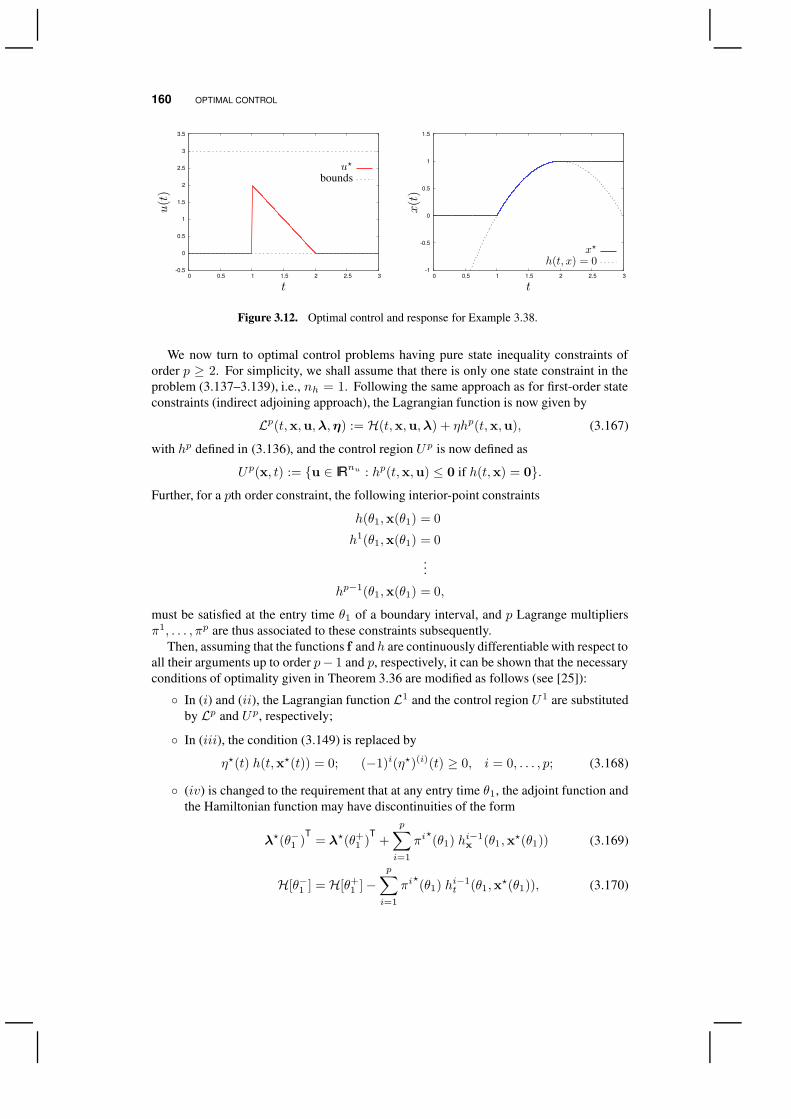
160 OPTIMAL CONTROL
-0.5
0
0.5
1
1.5
2
2.5
3
3.5
0 0.5 1 1.5 2 2.5 3
PSfrag replacements
t
u(t
)
x(t)
bounds
h(t, x) = 0
u?
x?-1
-0.5
0
0.5
1
1.5
0 0.5 1 1.5 2 2.5 3
PSfrag replacements
t
u(t)
x(t
)
boundsh(t, x) = 0
u?
x?
Figure 3.12. Optimal control and response for Example 3.38.
We now turn to optimal control problems having pure state inequality constraints oforder p ≥ 2. For simplicity, we shall assume that there is only one state constraint in theproblem (3.137–3.139), i.e., nh = 1. Following the same approach as for first-order stateconstraints (indirect adjoining approach), the Lagrangian function is now given by
Lp(t,x,u,λ,η) := H(t,x,u,λ) + ηhp(t,x,u), (3.167)
with hp defined in (3.136), and the control region U p is now defined as
Up(x, t) := u ∈ IRnu : hp(t,x,u) ≤ 0 if h(t,x) = 0.Further, for a pth order constraint, the following interior-point constraints
h(θ1,x(θ1) = 0
h1(θ1,x(θ1) = 0
...
hp−1(θ1,x(θ1) = 0,
must be satisfied at the entry time θ1 of a boundary interval, and p Lagrange multipliersπ1, . . . , πp are thus associated to these constraints subsequently.
Then, assuming that the functions f and h are continuously differentiable with respect toall their arguments up to order p− 1 and p, respectively, it can be shown that the necessaryconditions of optimality given in Theorem 3.36 are modified as follows (see [25]):
In (i) and (ii), the Lagrangian function L1 and the control region U 1 are substitutedby Lp and Up, respectively;
In (iii), the condition (3.149) is replaced by
η?(t) h(t,x?(t)) = 0; (−1)i(η?)(i)(t) ≥ 0, i = 0, . . . , p; (3.168)
(iv) is changed to the requirement that at any entry time θ1, the adjoint function andthe Hamiltonian function may have discontinuities of the form
λ?(θ−1 )T
= λ?(θ+1 )T
+
p∑
i=1
πi?(θ1) h
i−1x (θ1,x
?(θ1)) (3.169)
H[θ−1 ] =H[θ+1 ]−p∑
i=1
πi?(θ1) h
i−1t (θ1,x
?(θ1)), (3.170)
NUMERICAL METHODS FOR OPTIMAL CONTROL PROBLEMS 161
where the Lagrange multipliers π1?(θ1), . . . , πp?(θ1) satisfy the conditions
πi?(θ1) h(θ1,x
?(θ1)) = 0, πi?(θ1) ≥ 0, i = 1, . . . , p; (3.171)
Moreover, at any contact time θc, (3.169), (3.170), and (3.171) hold with πi(θc) = 0,for i ≥ 2, and we have the additional conditions
πi?(θc)
≥=
(−1)p−i(η?)(p−k)(θ+c ), for
i = 1,i = 2, . . . , p;
(3.172)
(v) remains unchanged.
Note that all of the above conditions can be generalized readily to problems havingmultiple state inequality constraints h1(t,x(t)) ≤ 0, . . . , hnh(t,x(t)) ≤ 0, possibly ofdifferent orders p1, . . . , pnh .11 In particular, these conditions remain valid in the first-ordercase p1 = · · · = pnh = 1, and thus encompass those given in Theorem 3.36.
Finally, we close the discussion on high-order inequality state constraints by reemphasiz-ing the fact that such constraints give rise to highly complex, possibly ill-behaved, controlproblems. Similar to high-order singular control problems (e.g., the Fuller problem, see
3.5.4), an optimal control may exhibit a chattering behavior near high-order boundary arcs(either at the entry or at the exit point), i.e., the costate variables may have countably manyjumps. An example of this behavior can be found in [43], for a problem having a third-orderinequality state constraint.
3.6 NUMERICAL METHODS FOR OPTIMAL CONTROL PROBLEMS
Unless the system equations, along with the cost functional and the constraints, of theproblem at hand are rather simple, numerical methods must be employed to solve optimalcontrol problems. With the development of economical, high speed computers over the lastfew decades, it has become possible to solve complicated problems in a reasonable amountof time.
Presenting a survey of numerical methods in the field of optimal control is a dauntingtask. Perhaps the most difficult aspect is restricting the scope of the survey to permit ameaningful discussion within a few pages only. In this objective, we shall focus on twotypes of numerical methods, namely, direct solution methods ( 3.6.3) and indirect solutionmethods ( 3.6.2). The distinction between direct and indirect methods can be understoodas follows. A direct method attempts to find a minimum to the objective function in thefeasible set, by constructing a sequence of points converging to that minimum. In contrast,an indirect method attempts to find a minimum point ’indirectly’, by solving the necessaryconditions of optimality. For this reason, indirect methods are often referred to as PMP-based methods or variational methods in the literature. Other approaches not discussedherein include dynamic programming methods [18, 37] and stochastic optimization methods[5].
In many numerical methods, one needs to calculate the values of functionals subject tothe differential equations. Moreover, since these functionals depend on parameters (e.g.,as a result of the parameterization of the control trajectories), there is much interest inevaluating their gradients with respect to the parameters. Before presenting the numerical
11A complex example involving a state third-order inequality constraint, two first-order inequality constraints, anda control constraint can be found in [13].
162 OPTIMAL CONTROL
methods for optimal control, we shall therefore give a close look to the evaluation ofparameter-dependent functionals and their gradients in 3.6.1.
3.6.1 Evaluation of Parameter-Dependent Functionals and their Gradients
In this subsection, our focus is on a Mayer type functional F defined as
F(p) := φ(x(tf),p), (3.173)
where p ∈ P ⊂ IRnp is a vector of time-invariant parameters, and the state x(t) ∈ IRnx isdescribed by a set of parametric ODEs
x(t) = f(t,x,p), t0 ≤ t ≤ tf; x(t0) = h(p). (3.174)
In what follows, `, f and h are always assumed continuous in (t,x,p) with continuous firstpartial derivatives with respect to (x,p), for (t,x,p) ∈ [t0, tf] × IRnx × P . Remind thatboth Lagrange and Bolza type functionals can be converted into the Mayer form by addingan extra state variable and differential equation to (3.174) that correspond to the integrandof the integral term, and then considering the value of this extra state at final time (see 3.2.3on p. 108).
Assuming that a unique solution x(t;p) to the system (3.174) exists for a given p ∈ P ,we wish to calculate the value F(p) as well as its gradient ∇pF(p). Obtaining F(p)requires that the IVP (3.174) be numerically integrated, and a brief overview of numericalmethods for IVPs in ODEs is thus given in 3.6.1.1. On the other hand, the computationof ∇pF(p) is less straightforward, and we shall present three methods for doing this: thefinite differences approach ( 3.6.1.2), the sensitivity approach ( 3.6.1.3), and the adjointapproach ( 3.6.1.4).
3.6.1.1 Initial Value Problems The problem of evaluating the functional F for givenvalues p ∈ P of the parameters consists of computing the value of x(tf) that satisfies
x(t) = f (t,x,p),
for each t0 ≤ t ≤ tf, from the initial value x(t0) = h(p). Numerical methods forsolving the foregoing IVP are relatively mature in comparison to other fields in numericaloptimization. Any numerical methods for ODEs generate an approximate solution step-by-step in discrete increments across the interval of integration, in effect producing a discretesample of approximate values xi of the solution function x(t). Most schemes can beclassified as either one-step or multi-step methods.12
One-Step Methods. A popular family of one-step methods is the Runge-Kutta (RK)schemes. Given an estimate xi of the states at time ti, an new estimate xi+1 at timeti+1 := ti + hi is obtained as
xi+1 = xi +K∑
j=1
ωjf ij ,
wheref ij := f
(
ti + hiτi,xi + hi
∑Kk=1 αjkf ik,p
)
, 1 ≤ j ≤ K,
12An excellent website illustrating numerical methods for solving IVPs in ODEs can be found at http://www.cse.uiuc.edu/eot/modules/ode/.
NUMERICAL METHODS FOR OPTIMAL CONTROL PROBLEMS 163
with 0 ≤ τ1 ≤ · · · ≤ τK ≤ 1, andK ≥ 1 denotes the number of stages in the scheme. RKschemes differ in the choice of the parameters ωi, τi, and αij , which are most convenientlyrepresented in the so-called Butcher diagram:
ω1 α11 · · · α1K
......
. . ....
ωK αK1 · · · αKK
β1 · · · βK
RK schemes are said to be explicit if the Butcher diagram is such that αjk = 0 for j ≤ k),and implicit otherwise. Three common examples of RK schemes are the following:
Euler’s Explicit: Classical Runge-Kutta Explicit: Trapezoidal Implicit:K = 1 K = 4 K = 2
0 0
1
0 0 0 0 012
12 0 0 0
12 0 1
2 0 0
1 0 0 1 0
16
13
13
16
0 0 0
1 12
12
12
12
An obvious appeal of an explicit scheme is that the computation of each integration stepcan be performed without iteration; that is, given the value of xi at time ti, the value ofxi+1 at the next time ti+1 follows directly from available values of f . In contrast, for animplicit scheme, the unknown value xi+1 appears nonlinearly, e.g., the Hermite-Simpsonimplicit method requires
Fi := xi+1 − xi − hi2
[
f (ti+1,xi+1,p) + f(ti,x
i,p)]
= 0. (3.175)
Computing xi+1 from given values of ti, ti+1 and xi thus requires solving the nonlinearexpression (3.175) to drive the defect Fi to zero. The iterations required to solve thisequation are called the corrector iterations. An initial guess to begin the iteration is usuallyprovided by a so-called predictor step. There is considerable latitude in the choice ofpredictor and corrector schemes. For some well-behaved differential equations, a singlepredictor/corrector step is required. On the other hand, it may be necessary to performmultiple corrector iterations when the differential equations are stiff;13 this is generallydone based on Newton’s method (see 1.8.2, p. 34).
Linear Multi-step Methods. The general form of a K-step linear multi-step method isgiven by
xi+1 =
K∑
j=1
αjxi−j+1 + h
K∑
j=0
βjfi−j+1, (3.176)
13An ODE whose solutions decay rapidly towards a common, slowly-varying solution is said to be stiff. Explicitmethods are generally inefficient for solving stiff ODEs because their stability region is relatively small, whichforces the step size to be much smaller than that required to achieve the desired accuracy. Implicit methods requiremore work per step, but their significantly larger stability regions permit much larger steps to be taken, so theyare often much more efficient than explicit methods of comparable accuracy for solving stiff ODEs. (A numericalmethod is said to be stable if small perturbations do not cause the resulting numerical solutions to diverge withoutbound.)
164 OPTIMAL CONTROL
where αj and βj are specified constants, xi is the approximate solution at time ti, andf i := f (ti,x
i,p). If βN = 0, the method is explicit, otherwise it is implicit. Note that theK-past integration steps are assumed to be equally spaced.
The most popular linear multi-step methods are based on polynomial interpolation, andeven methods which are not based on interpolation use interpolation for such purposes aschanging the step size. These methods come in families. Particularly popular for non-stiffproblems is the Adams family, and for stiff problems, the backward differentiation formula(BDF) family.
In a K-step Adams-Bashforth method, the solution is advanced at each step by inte-grating the interpolant of the derivative values atK previous solution points. Specif-ically, for approximate solution points (ti−K+1,x
i−K+1), . . . , (ti,xi), the approxi-
mate solution value xi+1 at time ti+1 = ti + h is given by
x(ti+1) = x(ti) +
∫ ti
ti+1
F(t) dt,
where F(t) is the unique polynomial of degree K − 1 interpolatingf(ti−K+1,x
i−K+1,p), . . . , (ti,xi,p). That is, we have α1 = 1, and αj = 0 for
j > 1, in the general form (3.176). A K-step Adams-Moulton method is derivedsimilarly to a Adams-Bashforth method, except that it interpolates f at the unknownvalue ti+1 as well.
In a K-step BDF method, the solution is advanced at each step by interpolating Kprevious solution points along with the (as yet unknown) new solution point, differ-entiating that interpolant, and requiring the derivative to match the ODE at the newpoint. Specifically, for approximate solution points (ti−K+1,x
i−K+1), . . . , (ti,xi),
the approximate solution value xi+1 at time ti+1 = ti + h is determined by solvingthe implicit equation
X(ti+1) = f(ti+1,xi+1,p)
for xi+1, where X(t) is the unique polynomial of degree K that interpolates(ti−K+1,x
i−K+1), . . . , (ti,xi), (ti+1,x
i+1). Hence, we have β0 6= 0, and βj = 0for j > 1, in the general form (3.176). Note that the simplest member of this familyis the implicit Euler method (i.e., α1 = 1 and β0 = 1):
xi+1 = xi + hf i+1.
BDF methods have relatively large stability regions, so they are particularly suitablefor solving stiff ODEs.
For a K-step method, the method is applied for i ≥ K − 1, and K initial valuesx0, . . . ,xK−1 are needed to start it up. A usual strategy is at a starting point is to graduallyincrease the method’s number of steps, starting fromK = 1. Another approach consists ofusing an appropriate RK method.
Differential-Algebraic Equations. Up to this point, the prototypical IVP (3.174) refersto an explicit ODE system,
x(t) = f(t,x(t),p). (3.177)
NUMERICAL METHODS FOR OPTIMAL CONTROL PROBLEMS 165
However, a more general formulation for an ODE system is the so-called implicit form,
F(t,x(t), x(t),p) = 0,
where the Jacobian matrix Fx is assumed to be nonsingular for all argument values in anappropriate domain. In principle, it is often possible to solve for x in terms of t, x and p,obtaining the explicit form (3.177). However, this transformation may not always be easyor cheap to realize. Also, in general, there may be additional questions of existence anduniqueness of the solutions.
Another extension of explicit ODEs is in systems of the form
x(t) = f (t,x(t),y(t),p) (3.178)0 = g(t,x(t),y(t),p), (3.179)
where the ODEs (3.178) now depend on additional variables y(t), and the pair (x(t),y(t))is forced to satisfy the algebraic constraints (3.179). Such systems are called differentialalgebraic equations (DAEs) in semi-explicit form. More generally, DAEs can be specifiedin fully-implicit form,
F(t, z(t), z(t),p) = 0, (3.180)
with the new variable zT := (xT,yT), and where the Jacobian matrix Fz is now singular.Note that the general theory for DAEs is much more recent and less developed than
for ODEs, and it is still subject to intense research activity [11]. Since a DAE involves amixture of differential and algebraic equations, one may hope that applying analytical timedifferentiations to a given system and eliminating, as needed, repeatedly if necessary, willyield an explicit ODE system for all the unknown variables. This turns out to be the case inmost situations (unless the problem is singular). In particular, the number of differentiationsneeded for this transformation is called the index of the DAE system.14 According to thisdefinition, ODEs have index 0. An index-2 DAE system is illustrated in Example 3.39below.
Example 3.39 (Index-2 DAE System). Consider the DAE system
z1(t)− q(t) = 0
z1(t)− z2(t) = 0.
where q(t) is a given smooth function. Differentiating the first equation gives
z2(t) = z1(t) = q(t),
and, by differentiating the resulting equation, we then get
z2(t) = z1(t) = q(t).
Hence, the index is 2 since two rounds of differentiation were needed.
14Formally, the index of a DAE system of the form (3.180) is defined as the minimum number of times that part orall of the equations must be differentiated in order to obtain an ODE system.

166 OPTIMAL CONTROL
The index of a DAE system is closely connected to the question of initial conditionsspecification. While n initial conditions must be given to fully specify the solution of anODE system of size n, a DAE system of size n will in general havem degrees of freedom,with m being anywhere between 0 and n. Which m pieces of information are needed todetermine the DAE solution may be a difficult issue, or at least not immediately obvious. Inother words, one must specify consistent initial conditions in the sense that the constraints ofthe system must be satisfied. To illustrate it, consider the DAE system in Example 3.39. Thevariable z1 at initial time must satisfy the obvious constraint z1(t) = q(t), but there is alsoa hidden constraints z2(t) = q(t) which the solution must satisfy at any time. Therefore,the only possible consistent initial conditions are z1(t0) = q(t0), z2(t0) = q(t0), i.e., theDAE system has zero degree of freedom!
The special case of semi-explicit DAEs (3.178,3.179) is encountered in many practicalproblems. It is readily shown that a sufficient condition for semi-explicit DAEs to haveindex 1, is that the Jacobian matrix gy be nonsingular. In the index-1 case, one can thendistinguish between the differential variables x(t) and the algebraic variables y(t).
Remark 3.40 (Link between DAEs and the Euler-Lagrange Equations). The Euler-Lagrange equations (3.13–3.15), which are part of the necessary conditions of optimality foroptimal control problems, are DAEs in semi-explicit form. Provided that the Hamiltonianfunction is nonsingular (i.e.,Huu is not trivially equal to zero, see 3.5.4), these equationshave index 1, and the differential variables are thus clearly identified to be the states andadjoints, whereas the algebraic variables correspond to the controls. But if the Hamiltonianfunction is now singular, the Euler-Lagrange equations have high index (≥ 2), which impliesthat the problem contains hidden constraints. These extra constraints correspond preciselyto the equations defining the singular surface, i.e.,
Hu = 0,ddtHu = 0, . . . ,
d2p
dt2pHu = 0,
where p denotes the order of singularity. Obviously, there exists strong connections be-tween high-index Euler-Lagrange equations and singularity optimal control problems. Thesituation is similar for optimal control problems with high-order state inequality constraints(see 3.5.6).
Numerical methods for solving DAEs are mostly limited to index-1 systems. Fortunately,this is the case for many practical systems. For higher-index systems to be handled, itis necessary to first transform the DAEs into index-1 form (e.g., by applying successivedifferentiation), before a solution can be computed. The first general technique for solvingfully implicit index-1 DAEs was proposed by Gear in 1971, It utilizes BDF methods similarto those used for ODEs, i.e., the derivative z is replaced by the derivative of the polynomialinterpolating the solution computed over the preceding K-steps along with the (as yetunknown) new solution point. The simplest example of a BDF method is the implicit Eulermethod that replaces (3.180) with
F
(
ti+1, zi+1,
zi+1 − zi
h,p
)
= 0.
The resulting nonlinear system in the variable zi+1 is usually solved by some form ofNewton’s method at each time step.
Implementation and Software. Regardless of whether a one-step or multi-step methodis utilized, a successful implementation must address the accuracy of the solution. How

NUMERICAL METHODS FOR OPTIMAL CONTROL PROBLEMS 167
well does the discrete solution xi for i = 0, 1, . . ., produced by the integration schemeagree with the true solution x(t)? All well-implemented integration schemes incorporatesome mechanism for adjusting the integration step-size and/or the order of the method tocontrol the integration error.15
A variety of excellent and widely used software for IVPs is readily available. Majordifferences between codes lie in the numerical scheme used, whether index-1 DAEs can beaccommodated, and whether sparse systems can be handled efficiently (especially usefulfor large-scale systems). A number of free numerical integration codes is given in Tab. 3.1.
Table 3.1. Popular codes doing numerical integration of ODEs/DAEs.
Solver Website Lic. Characteristics
DASSL http://www.engineering.ucsb.edu/
~cse/software.html
free BDF schemes, ODEs and index-1 DAEs,dense or banded Jacobian
DASPK2.0 http://www.engineering.ucsb.edu/
~cse/software.html
free same as DASSL, designed for sparse,large-scale systems
CVODE http://acts.nersc.gov/sundials/ free Adams-Moulton and BDF schemes,ODEs only, designed for dense or sparse,large-scale systems
IDA http://acts.nersc.gov/sundials/ free BDF schemes, ODE and index-1 DAEproblems, consistent initialization
The codes listed in Tab. 3.1. are stand-alone (either in C or fortran77). Moreover,various integration schemes are available in the MATLAB environment, both for ODEs(Runge-Kutta, Adams, BDF schemes) and index-1 DAEs (BDF schemes).
3.6.1.2 Gradients via Finite Differences We now turn to the problem of calculat-ing the gradient ∇pF(p) of the functional (3.173), subject to the IVP in ODEs (3.174).The easiest way of getting an estimate of ∇pF(p) is to consider a forward differenceapproximation so that:
∇pjF(p) ≈F(p1, . . . , pj + δpj , . . . , pnp)− F(p)
δpj, (3.181)
for each j = 1, . . . , np. In practice, the variations δpj can be chosen as
δpj = εa + pjεr,
where εa and εr are small absolute and relative perturbations parameters, respectively; often,εa and εr are chosen as the square-roots of the absolute and relative tolerances used in thenumerical integration code.
A practical procedure for calculating both the value and the gradient of F is as follows:
Initial StepIntegrate the ODEs (3.174) once with the actual parameter values p;Calculate the value of F(p).
Loop: j = 1, . . . , np
15It should be stressed that error control mechanism in numerical integration schemes is inherently local, i.e., itcan only guarantee the accuracy of the solution from one step to the next. That is, if the numerical scheme takesmany integration steps, the error accumulates and there is no guarantee that the discrete solution will be a goodapproximation or even close to the desired solution in the end.

168 OPTIMAL CONTROL
Set pi := pi, i 6= j; pj := pj + δpj ;Integrate the ODEs (3.174) once with the perturbed parameter values p;Calculate the value of F(p), and
∇pjF(p) ≈ F(p)− F(p)
δpj.
End Loop
Observe that a gradient calculation with the forward difference approach requires np+1integrations of the ODEs (3.174), which can be computationally expensive when np islarge. On the other hand, however, this approach does not bring any additional complexityother than integrating the ODEs for the system, and applies readily to the case of (index-1)DAEs. A more accurate approximation (2nd-orderapproximation)can be obtained by usingcentered finite differences as
∇pjF(p) ≈F(p1, . . . , pj + δpj , . . . , pnp)− F(p1, . . . , pj − δpj , . . . , pnp)
2δpj, (3.182)
although this requires 2 functional evaluations per parameter, i.e., an overall 2× np ODEsintegrations for a single gradient evaluation.
A major limitation of the finite differences approach lies in its accuracy. It is easy tosee why the difference formulas (3.181) do not provide accurate values. If δpj is small,then cancellation error reduces the number of significant figures in the gradient estimate,especially when the function values are obtained with limited accuracy from a numericalintegration code. On the other hand, if δpj is not small, then truncation errors (i.e., higher-order terms) become significant. Even if δpj is optimally chosen, it is well known that∇pF(p) will be accurate to only about 1
2 of the significant digits of F(p) (or 23 if the cen-
tered formula (3.182) is used). This motivates the forward and adjoint (reverse) sensitivityapproaches of gradient calculation presented subsequently.
3.6.1.3 Gradients via Forward Sensitivity Analysis Consider the IVP in ODEs(3.174) for given parameter values p ∈ P ,
x(t;p) = f(t,x(t;p),p); x(t0;p) = h(p). (3.183)
and suppose that (3.183) has a unique solution x(t;p), t0 ≤ t ≤ tf. The functions f andh being continuously differentiable with respect to (x,p) and p, respectively, the solutionx(t;p) of (3.174) is itself continuously differentiable with respect to p in a neighborhoodof p, at each t ∈ [t0, tf] (see Appendix A.5.3). In particular, the first-order state sensitivityfunctions xpj (t;p), j = 1, . . . , np, are given by (A.15), or equivalently,
xpj (t;p) = fx(t,x(t;p),p) xpj (t;p) + fpj (t,x(t;p),p); xpj (t0;p) = hpj (p).(3.184)
The foregoing equations are called the sensitivity equations with respect to parameter pj ; ingeneral, they are linear, non-homogeneous differential equations,and become homogeneousin the case where f pj = 0.
Once the state sensitivity functions are known at t = tf, and since φ is continuouslydifferentiable with respect to x and p, the gradient ∇pF(p) of the functional (3.173) at pcan be calculated as
∇pjF(p) = φx(x(tf;p),p)Txpj (tf;p) + φpj (x(tf;p),p), (3.185)
NUMERICAL METHODS FOR OPTIMAL CONTROL PROBLEMS 169
for each j = 1, . . . , np.A practical procedure calculating both the value and the gradient of F at p is as follows:
State and Sensitivity Numerical Integration: t0 → tf
x(t) = f(t,x(t),p); x(t0) = h(p)
xp1(t) = fx(t,x(t),p) xp1(t) + fp1(t,x(t),p); xp1(t0) = hp1(p)
......
xpnp (t) = fx(t,x(t),p) xpnp (t) + f pnp (t,x(t),p); xpnp (t0) = hpnp (p)
Function and Gradient Evaluation:
F(p) = φ(x(tf),p)
∇p1F(p) = φx(x(tf),p)Txp1(tf) + φp1(x(tf),p)
...
∇pnpF(p) = φx(x(tf),p)Txpnp (tf) + φpnp (x(tf),p)
Observe that the state and state sensitivity equations are solved simultaneously, so thata local error control can be performed on both the state and state sensitivity variables.However, the size of the state/sensitivity system grows proportionally to the number ofstates and parameters as (nx + 1) × np, which can lead to computationally intractableproblems if both nx and np are large. In response to this, effective methods have beendeveloped in recent years that take advantage of the special structure of the problem. Thesemethods are usually based on implicit multi-step integration schemes (see 3.6.1.1, 163),and exploit the fact that the sensitivity equations (3.184) are linear and all share the sameJacobian matrix with the original system (3.183). Three well-established methods, whichdiffer in the way the corrector formula is solved while sharing the same predictor step, arethe following:
Staggered direct methods [31]: At each time step, the states are computed first bythe nonlinear corrector step, and the state sensitivities are then obtained by solvinga linear system. This method is sometimes considered to be inefficient because itrequires that the Jacobian matrix be evaluated and factored16 at every time step.
Simultaneous corrector methods [39]: The state and sensitivity variables are com-puted simultaneously by the nonlinear corrector step. This method is more efficientbecause it evaluates and factors the Jacobian matrix only when necessary.
Staggered corrector method [20]: This method is similar to the staggered directmethod, except that it uses the factorization of the Jacobian matrix at some past stepto solve the linear sensitivity system. This saves on the number of factorizations ofthe Jacobian matrix, which can be the most expensive part of the computations forsystems having many state variables but relatively few parameters.
16Here, we refer to the LU factorization of the Jacobian matrix, which is used in the corrector step for calculatingthe inverse of the Jacobian matrix

170 OPTIMAL CONTROL
Note that all these methods apply equally well for fully implicit, index-1 DAE systemsof the form (3.180). In this case the sensitivity DAEs read:
Fx xpj + Fx xpj + Fpj = 0, (3.186)
for each j = 1, . . . , np. Obviously, consistent initial state sensitivities must be specified tothe sensitivity DAEs; they are obtained upon direct differentiation of the initial conditionsof the original DAEs.
A variety of excellent and widely used codes is available for forward sensitivity analysisof IVPs in ODEs and DAEs, such as those listed in Tab. 3.2. hereafter. Note that the version7.4 of MATLAB does not have a function doing forward sensitivity analysis.
Table 3.2. Popular codes doing forward sensitivity analysis of ODEs/DAEs.
Solver Website Lic. Characteristics
DSL48S http://yoric.mit.edu/dsl48s.html free foracad.
based on DASSLa, ODEs and index-1DAEs, sparse Jacobian
DASPK3.0 http://www.engineering.ucsb.edu/
~cse/software.html
free foracad.
based on DASSLa, ODEs, index-1DAEs and Hessenberg index-2 DAEs
CVODES http://acts.nersc.gov/sundials/ free based on CVODEa, ODEs only
aSee Tab. 3.1.
3.6.1.4 Gradients via Adjoint Sensitivity Analysis Some problems require thegradient of a functional with respect to a large number of parameters. For these problems,particularly if the number of state variables is also large, both the finite differences approach( 3.6.1.2) and the forward sensitivity approach ( 3.6.1.3) are intractable. This motivates thethird class of methods, namely adjoint sensitivity analysis (also called reverse sensitivityanalysis), for computing the gradient of a functional [19].
Consider the functional (3.173), subject to the IVP in ODEs (3.174), at a point p ∈ P .Analogous to 3.6.1.3, we shall suppose that (3.183) has a unique solution x(t;p), t0 ≤t ≤ tf. Then, adjoining the differential equations to the functional using smooth multiplierfunctions λ ∈ C1[t0, tf]
nx , we form the augmented functional
F(p) := φ(x(tf;p),p) +
∫ tf
t0
λ(t)T [f(t,x(t;p),p)− x(t,p)] dt.
Since x = f (t,x,p) at each t ∈ [t0, tf], the gradient ∇pjF(p), i = 1, . . . , np, is obtainedby applying the chain rule of differentiation:
∇pjF(p) =∇pj F(p) (3.187)
= φpj (x(tf),p) + φx(x(tf),p)Txpj (tf) (3.188)
+
∫ tf
t0
λ(t)T [
fpj (t,x(t),p) + fx(t,x(t),p) xpj (t)− xpj (t)]
dt.
By integration by parts, we have∫ tf
t0
λ(t)Txpj (t) dt =
[
λ(t)Txpj (t)
]tf
t0−∫ tf
t0
λ(t)Txpj (t) dt.

NUMERICAL METHODS FOR OPTIMAL CONTROL PROBLEMS 171
Thus, (3.188) becomes
∇pjF(p) = φpj (x(tf),p) + λ(t0)Thpj (p) + [φx(x(tf),p)− λ(tf)]
Txpj (tf)
+
∫ tf
t0
[
λ(t)Tfpj (t,x(t),p) +[
fx(t,x(t),p)Tλ(t) + λ(t)
]Txpj (t)
]
dt.
The foregoing expression being verified for any smooth function λ(·), it is convenient tochoose λ(·) so as to eliminate the terms depending on the sensitivity variables xpj :
λ?(t) = −fx(t,x(t),p)
Tλ?(t); λ?(tf) = φx(x(tf),p),
from which we obtain
∇pjF(p) = φpj (x(tf),p) + λ?(t0)Thpj (p) +
∫ tf
t0
λ?(t)Tfpj (t,x(t),p) dt. (3.189)
for each j = 1, . . . , np. Interestingly, the expression of ∇pjF(p) can be seen as the sumof 3 contributions: (i) the direct influence of the parameter pj on the cost functional; (ii)the influence of pj through the initial conditions; and (iii) the influence of pj through thesystem dynamics.
A practical procedure for calculating both the value and the gradient of F at p is asfollows:
State Numerical Integration: t0 → tf
x(t) = f(t,x(t),p); x(t0) = h(p);
Store the state values x(t) at mesh points, t0 < t1 < t2 < · · · < tM = tf.
Adjoint Numerical Integration: tf → t0
λ(t) = − fx(t,x(t),p)Tλ(t); λ(tf) = φx(x(tf),p)
q1(t) = − f p1(t,x(t),p)Tλ(t); q1(tf) = 0
...
qnp(t) = − f pnp (t,x(t),p)Tλ(t); qnp(tf) = 0;
Evaluate the right-hand-sides of the adjoint equations by interpolating the state valuesx(t), tk ≤ t ≤ tk+1, between mesh points x(tk) and x(tk+1).
Function and Gradient Evaluation:
F(p) = φ(x(tf),p)
∇p1F(p) = φp1 (x(tf),p) + λ?(t0)Thp1(p) + q1(t0)
...
∇pnpF(p) = φpnp (x(tf),p) + λ?(t0)Thpnp (p) + qnp(t0)

172 OPTIMAL CONTROL
In number of remarks are in order. The state and adjoint equations are integrated forwardand backward in time, respectively, from their natural initial/terminal conditions. This way,the adjoint equations are stable provided that the state equations are themselves stable [15].However, integrating the adjoint equations backward in time requires that the state valuesbe “reconstructed” at each time instant. This can be done by storing all the necessaryinformation about the state variables at each time step during the forward integration,and then interpolating these values during the backward integration; possible interpolationschemes are linear interpolation (requires x(t) at each time step only), or cubic Hermiteinterpolation (requires both x(t) and x(t) at each time step).
It is convenient to introduce quadrature variables qi, i = 1, . . . , np, and appending thecorresponding equations to the adjoint system, for calculating the integral term in (3.189).Most numerical solver allow dealing with quadrature variables very efficiently since theydo not enter into the Jacobian matrix.
In terms of computational efficiency, the cost of the forward sensitivity method ( 3.6.1.3)is roughly proportional to the number np of sensitivity parameters, and is insensitive tothe number of functionals (e.g., F1, . . . ,FnF
). For the adjoint sensitivity method, on theother hand, the computational cost is proportional to the number nF of functionals andis insensitive to the number np of parameters. The adjoint sensitivity method is there-fore advantageous over the forward sensitivity method when the number of sensitivityparameters is large, and the number of functionals is small. Observe also that the adjointsensitivity method has a disadvantage that it can only compute the gradient of a specifiedfunctional;,unlike the forward sensitivity approach which provide the state sensitivities atany time, the intermediate results of the adjoint variables cannot be exploited.
Remark 3.41 (Extension to Functionals Defined at Multiple Time Instants). A usefulextension of the adjoint sensitivity method described previously is in the situation wherethe functional depends on the state values at multiple (fixed) time instants,17
F′(p) :=
N∑
k=1
φk(x(tk),p), (3.190)
where t0 < t1 < t2 < · · · < tN = tf, subject to the IVP in ODEs (3.174). It can be shownthat the gradient ∇pjF
′(p), i = 1, . . . , np, at p ∈ P is given by
∇pjF(p) =
N∑
k=1
[
φkpj (x(tk),p) +
∫ tk
tk−1
λ?(t)Tfpj (t,x(t),p) dt
]
+ λ?(t0)Thpj (p),
where the adjoint variables λ? are the solutions to the ODEs
λ?(t) = −fx(t,x(t),p)
Tλ?(t),
from the terminal conditionλ?(tN ) = φNx (x(tN ),p),
and satisfying the jump conditions
λ?(t−k ) = λ?(t+k ) + φkx(x(tk),p).
17Such functionals arise frequently, e.g., in parameter identification problems where the objective is to calculatethe parameter values minimizing the gap between a set of measurements and the model prediction, at given timeinstants.
NUMERICAL METHODS FOR OPTIMAL CONTROL PROBLEMS 173
The extension of the adjoint method to the case of index-1, fully implicit DAE systemshas also been proposed recently (see [15] for details).
Although they are less straightforward to implement than forward sensitivity methods,mainly due to the need to store the state profile, adjoint methods are not difficult to automate.Several codes are available for adjoint sensitivity analysis of IVPs in ODEs and DAEs. Welist some of these codes in Tab. 3.2. below. Note that the version 7.4 of MATLAB doesnot have a function doing adjoint sensitivity analysis.
Table 3.3. Popular codes doing adjoint sensitivity analysis of ODEs/DAEs.
Solver Website Lic. Characteristics
DASPKadjoint http://www.engineering.ucsb.edu/
~cse/software.html
free foracad.
based on DASPK3.0a (still underdevelopment)
CVODES http://acts.nersc.gov/sundials/ free based on CVODEb, ODEs only
aSee Tab. 3.2.bSee Tab. 3.1.
3.6.2 Indirect Methods
Having presented numerical methods for calculating the values and gradients of generalfunctionals, we are now ready to investigate numerical methods for solving optimal controlproblems. Our focus in this subsection is on indirect methods. Essentially, indirect methodsattempt to solve optimal control problems by seeking a solution to the (closed system of)necessary conditions of optimality (NCOs), such as those presented earlier in 3.4 and 3.5.
Many indirect methods use iterative procedures based on successive linearization to finda solution to the system of NCOs. A nominal solution is chosen that satisfies part of theNCOs, then this nominal solution is modified by successive linearization so as to meet theremaining NCOs. Popular indirect methods for optimal control include quasi-linearizationmethods, gradient methods such as control vector iteration, and indirect shooting methods(see [12]). Only the latter class of methods shall be considered herein. We shall firstpresent the indirect shooting method for optimal control problems having terminal equalityconstraints only ( 3.6.2.1), and then discuss its extensions to encompass problems withterminal and/or path inequality constraints ( 3.6.2.2).
3.6.2.1 Indirect Shooting Methods To set forth the basic ideas of indirect shootingmethods, we consider first the relatively simple class of problems treated in 3.4.5: Findu? ∈ C1[t0, T ]nu and t?f ∈ [t0, T ) to
minimize: J(u, tf) :=
∫ tf
t0
`(t,x(t),u(t)) dt+ φ(tf,x(tf)) (3.191)
subject to: x(t) = f (t,x(t),u(t)); x(t0) = x0 (3.192)ψk(tf,x(tf)) = 0, k = 1, . . . , nψ. (3.193)
Provided that the problem (3.191–3.193) is normal and (u?, t?f ) is an optimal solution,there must exist a quintuple (u?(·),x?(·),λ?(·),ν?, t?f ) which satisfies the Euler-Lagrange
174 OPTIMAL CONTROL
equations
x?(t) =Hλ(t,x?(t),u?(t),λ?(t)); x?(t0) = x0 (3.194)
λ?(t) = −Hx(t,x?(t),u?(t),λ?(t)); λ?(t?f ) = Φx(t?f ,x
?(t?f )) (3.195)0 =Hu(t,x(t),u(t),λ(t)), (3.196)
for all t0 ≤ t ≤ t?f , along with the transversal conditions
ψ(t?f ,x?(t?f )) = 0 (3.197)
Φt(t?f ,x(t?f )) +H(t?f ,x
?(t?f ),u?(t?f ),λ
?(t?f )) = 0, (3.198)
with Φ := φ+ ν?Tψ andH := `+ λ?Tf .
Observe that if the adjoint values λ?(t0) at initial time, the Lagrange multipliers ν?,and the terminal time t?f were known, the Euler-Lagrange equations could be integrated,all together, forward in time. Hence, the idea of indirect shooting is to guess the valuesof λ?(t0), ν?, and t?f , and then iteratively improve these estimates to satisfy the adjointterminal conditions and the transversal conditions. (For this reason, this approach is alsoreferred to as boundary conditions iteration (BCI) in the literature.) In other words, onewants to find (λ?(t0),ν
?, t?f ) such that
b(λ?(t0),ν?, t?f ) :=
λ? + φx + ν?Tφx
ψ
`+ λ?Tf + φt + ν?φt
t=t?f
= 0.
In particular, a Newton iteration can be used to improve the estimates. An algorithmimplementing the indirect shooting approach for optimal control problems having equalityterminal constraints is given in the following.
Initialization StepLet ε > 0 be a termination scalar, and choose initial values λ0
0, ν0, t0f . Let k = 0and go to the main step.
Main Step
1. Calculate the defect b(λk0 ,νk, tkf ) in the boundary and transversal conditions.
If ‖b(λk0 ,νk, tkf )‖ < ε, stop;
2. Calculate the gradients ∇λ0b(λk0 ,ν
k, tkf ), ∇νb(λk0 ,νk, tkf ),∇tfb(λk0 ,ν
k, tkf )of the defect;
3. Solve the linear system
∇λ0b(λk0 ,ν
k, tkf )T
∇νb(λk0 ,νk, tkf )
T
∇tfb(λk0 ,νk, tkf )
T
T
dkλdkνdktf
= −b(λk0 ,νk, tkf )
to get the directions dkλ, dkν and dktf.
NUMERICAL METHODS FOR OPTIMAL CONTROL PROBLEMS 175
4. Compute the new estimates
λk+10 = λk0 + dkλ
νk+1 = νk + dkν
tk+1f = tkf + dktf
.
5. Replace k ← k + 1, and go to step 1.
A number of remarks are in order.
Obviously, the same procedure applies in the absence of terminal constraints, or ifthe terminal time is fixed. It suffices to reduce the number of free variables, and keeponly the relevant necessary conditions in the defect function b.
Instead of iterating on the adjoint initial conditions λk0 , one may as well guess thestate terminal conditions xkf = xk(tkf ), and integrate the Euler-Lagrange equationsbackward in time (starting from the guessed terminal time tkf ).
At each Newton iterate, one must supply the gradient of the functionals b(λk0 ,νk, tkf ).
Although any of the methods described in 3.6.1.2 through 3.6.1.4 can be used, theforward sensitivity analysis approach is often the most efficient, since the number ofparameters is usually small, and there are as many functionals as parameters. Notethat, for problems with unspecified final time, it is necessary to make a change ofvariables so that the time range be fixed, e.g., to [0, 1]; this way, the final time t?fbecomes a parameter of the problem, and both the forward and adjoint sensitivityanalysis can be conducted. Yet another alternative to avoid gradient calculation is toapply a quasi-Newton method using a DFP or BFGS update scheme for estimatingthe Jacobian matrix. (see 1.8.3.2).
An illustration of the indirect shooting method is presented in Example 3.42 below.
Example 3.42 (Indirect Shooting Method). Consider the following scalar optimal controlproblem with terminal state equality constraint:
minimize: J(u) :=
∫ 1
0
12u(t)
2 dt (3.199)
subject to: x(t) = u(t)[1− x(t)]; x(0) = −1; x(1) = 0, (3.200)
with u ∈ C [0, 1]. Provided that u? is an optimal for this problem, there must exist aquadruple (u?, x?, λ?, ν?) such that
x?(t) = Hλ = u?(t)[1− x?(t)]; x?(0) = −1; x?(1) = 0
λ?(t) = −Hx = u?(t)λ?(t); λ?(1) = ν?
0 = Hu = u(t) + λ(t)[1− x(t)].We now apply the indirect shooting approach to find one such quadruple. A full-step Newtonalgorithm is used here to find the unspecified adjoint conditions λ?(0) and the Lagrangemultiplier ν? such that
b(λ?(0), ν?) =
(
λ(1)− νx(1)
)
= 0,
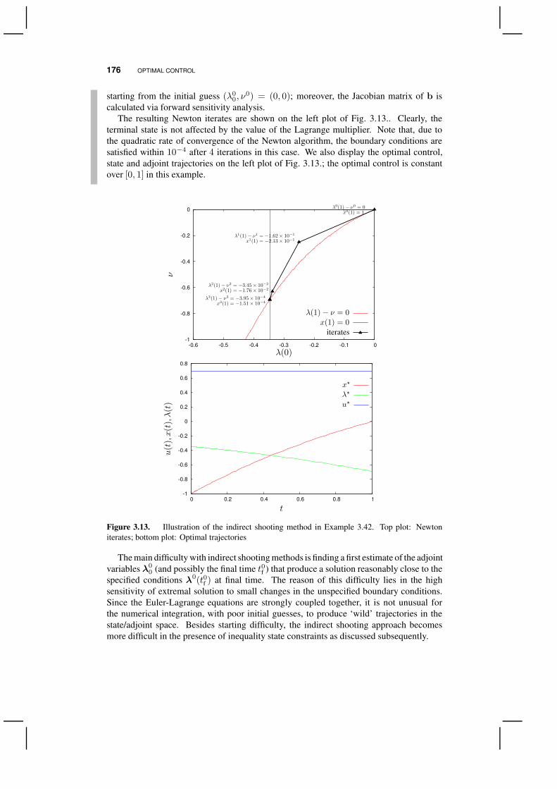
176 OPTIMAL CONTROL
starting from the initial guess (λ00, ν
0) = (0, 0); moreover, the Jacobian matrix of b iscalculated via forward sensitivity analysis.
The resulting Newton iterates are shown on the left plot of Fig. 3.13.. Clearly, theterminal state is not affected by the value of the Lagrange multiplier. Note that, due tothe quadratic rate of convergence of the Newton algorithm, the boundary conditions aresatisfied within 10−4 after 4 iterations in this case. We also display the optimal control,state and adjoint trajectories on the left plot of Fig. 3.13.; the optimal control is constantover [0, 1] in this example.
-1
-0.8
-0.6
-0.4
-0.2
0
-0.6 -0.5 -0.4 -0.3 -0.2 -0.1 0
PSfrag replacements
λ(0)
νλ(1)− ν
x(1)
λ(1)− ν = 0x(1) = 0
λ0(1)− ν0 = 0x0(1) = 1
λ1(1)− ν1 = −1.62× 10−1
x1(1) = −2.13× 10⁻¹
λ2(1)− ν2 = −3.45× 10−2
x2(1) = −1.76× 10⁻²
λ3(1)− ν3 = −3.95× 10−4
x3(1) = −1.51× 10⁻⁴t
u(t), x(t), λ(t)
x?
λ?
u?iterates
-1
-0.8
-0.6
-0.4
-0.2
0
0.2
0.4
0.6
0.8
0 0.2 0.4 0.6 0.8 1
PSfrag replacementsλ(0)
νλ(1)− ν
x(1)λ(1)− ν = 0
x(1) = 0λ0(1)− ν0 = 0
x0(1) = 1λ1(1)− ν1 = −1.62× 10−1
x1(1) = −2.13× 10⁻¹
λ2(1)− ν2 = −3.45× 10−2
x2(1) = −1.76× 10⁻²
λ3(1)− ν3 = −3.95× 10−4
x3(1) = −1.51× 10⁻⁴
t
u(t
),x(t
),λ(t
)
x?
λ?
u?
iterates
Figure 3.13. Illustration of the indirect shooting method in Example 3.42. Top plot: Newtoniterates; bottom plot: Optimal trajectories
The main difficulty with indirect shooting methods is finding a first estimate of the adjointvariables λ0
0 (and possibly the final time t0f ) that produce a solution reasonably close to thespecified conditions λ0(t0f ) at final time. The reason of this difficulty lies in the highsensitivity of extremal solution to small changes in the unspecified boundary conditions.Since the Euler-Lagrange equations are strongly coupled together, it is not unusual forthe numerical integration, with poor initial guesses, to produce ‘wild’ trajectories in thestate/adjoint space. Besides starting difficulty, the indirect shooting approach becomesmore difficult in the presence of inequality state constraints as discussed subsequently.
NUMERICAL METHODS FOR OPTIMAL CONTROL PROBLEMS 177
3.6.2.2 Indirect Shooting with Inequality State Constraints For those simpleoptimal control problems having no inequality constraints and whose solution consists of asingle arc, the indirect shooting method proceeds by iteratively refining the estimates of theadjoint variables at initial time, together with the Lagrange multipliers and the terminal time.The situation gets more complicated for problems containing either terminal or path inequal-ity constraints. In this case, one has to postulate the sequence of constrained/unconstrainedarcs and the active terminal constraints a priori, then calculate the control, state, adjoint,and multiplier functions that satisfy the Euler-Lagrange equations, and finally check thatthe multipliers satisfy all of the sign conditions. If part of the sign conditions are not met,then the postulated sequence of arcs cannot be optimal; a new sequence of arcs must beselected, and the optimization procedure is repeated until all the NCOs are satisfied.
Particularly difficult to solve are problems having inequality state constraints, since theadjoint trajectories may be discontinuous at the entry time of boundary arcs. In this case, thenecessary conditions of optimality yield a nonlinear multi-point boundary value problem(MPBVP), i.e., additional conditions must also hold at interior points (see 3.5.6).
Besides the need of specifying rather accurate estimates for the adjoint variables at initialtime and entry/contact times, another severe drawback of indirect shooting methods is thatdetailed a priori knowledge of the stucture of the optimal solution must be available. Inparticular, the direct methods presented in the following subsection do not require such an apriori knowledge, and can be used to identify the various types of arcs present in an optimalsolution, as well as the active set of terminal constraints.
3.6.3 Direct Methods
Numerical methods that avoid the drawbacks of indirect methods can be found in the so-called direct optimization methods, which have been studied extensively over the last 30years, and have proved to be powerful tools for solving practical optimal control problems.The basic idea of direct optimization methods is to discretize the control problem, and thenapply NLP techniques to the resulting finite-dimensional optimization problem. Thesemethods use only control and/or state variables as optimization variables and dispensecompletely with adjoint variables. Moreover, adjoint variables can be obtained by post-optimal calculations using the Lagrange multipliers of the resulting nonlinear optimizationproblem [14]. Another advantage is that they can be readily extended to problems describedby DAE systems. Of course, an obvious drawback of direct methods is that they providesuboptimal solutions only, due to the discretization of the control profiles.
In this section, we shall present two popular direct methods, namely, the sequentialmethod (3.6.3.1) and the simultaneous method (3.6.3.2), which differ in the level of dis-cretization. The pros and cons of either methods will be discussed, and several illustrativeexamples will be given. In order to set forth the principles of direct methods, we shallconsider the following optimal control problem throughout:

178 OPTIMAL CONTROL
Problem 3.43. Find u? ∈ C1[t0, tf]nu and v? ∈ IRnv to
minimize: J(u) :=
∫ tf
t0
`(t,x(t),u(t),v) dt+ φ(x(tf),v) (3.201)
subject to: x(t) = f(t,x(t),u(t),v); x(t0) = h(v) (3.202)ψj(x(tf),v) = 0, j = 1, . . . , nψ (3.203)κj(x(tf),v) ≤ 0, j = 1, . . . , nκ (3.204)gj(t,x(t),u(t),v) ≤ 0, j = 1, . . . , ng (3.205)
u(t) ∈ [uL,uU ], v ∈ [vL,vU ]. (3.206)
In this formulation, the optimization horizon is fixed. However, free final time problemscan be easily handled by normalizing the time horizon, and considering the actual final timetf as an extra time-invariant parameter in the time-invariant parameter vector v.
3.6.3.1 Direct Sequential Methods In direct sequential methods, the control vari-ables u(·) are parameterized by a finite set of parameters, and the optimization is carriedout in the parameter space; hence, this approach is often referred to as control vector pa-rameterization (CVP) in the literature.
A convenient way to parameterize the controls is by subdividing the optimization horizon[t0, tf] into ns ≥ 1 control stages,
t0 < t1 < t2 < · · · < tns = tf,
and using low-order polynomials on each interval, so that
u(t) = Uk(t,ωk), tk−1 ≤ t ≤ tk.
withωk ∈ IRnkω . Clearly, different orders may be used for different control variables and/orfor different control intervals. For simplicity, we shall assume here that the same polynomialorder M is employed for each control variable in all stages.
In practice, Lagrange polynomials are often employed to approximate the controls. Instage k, the jth control variable is then given by
uj(t) = Ukj (t,ωk) =M∑
i=0
ωkijφ(M)i (τ (k)), tk−1 ≤ t ≤ tk (3.207)
where τ (k) =t−tk−1
tk−tk−1∈ [0, 1] stands for the normalized time in stage k, and φ(M)
i (·)denotes the Lagrange polynomial of order M ,18
φ(M)i (τ) :=
1, if M = 0M∏
q=0q 6=i
τ − τqτi − τq
, if M ≥ 1, (3.208)
18Lagrange polynomials have the property that φ(M)i (τq) = δi,q . Hence, at each collocation point τq , q =
0, . . . , M , we have:uj(tk−1 + τq(tk − tk−1)) = ωk
qj .
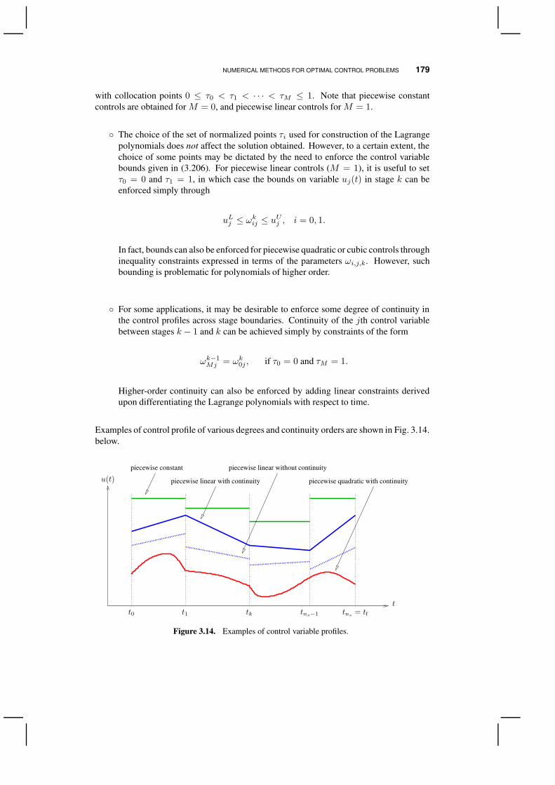
NUMERICAL METHODS FOR OPTIMAL CONTROL PROBLEMS 179
with collocation points 0 ≤ τ0 < τ1 < · · · < τM ≤ 1. Note that piecewise constantcontrols are obtained for M = 0, and piecewise linear controls for M = 1.
The choice of the set of normalized points τi used for construction of the Lagrangepolynomials does not affect the solution obtained. However, to a certain extent, thechoice of some points may be dictated by the need to enforce the control variablebounds given in (3.206). For piecewise linear controls (M = 1), it is useful to setτ0 = 0 and τ1 = 1, in which case the bounds on variable uj(t) in stage k can beenforced simply through
uLj ≤ ωkij ≤ uUj , i = 0, 1.
In fact, bounds can also be enforced for piecewise quadratic or cubic controls throughinequality constraints expressed in terms of the parameters ωi,j,k. However, suchbounding is problematic for polynomials of higher order.
For some applications, it may be desirable to enforce some degree of continuity inthe control profiles across stage boundaries. Continuity of the jth control variablebetween stages k − 1 and k can be achieved simply by constraints of the form
ωk−1Mj = ωk0j , if τ0 = 0 and τM = 1.
Higher-order continuity can also be enforced by adding linear constraints derivedupon differentiating the Lagrange polynomials with respect to time.
Examples of control profile of various degrees and continuity orders are shown in Fig. 3.14.below.
PSfrag replacements
t
u(t)
t0 t1 tk tns−1 tns = tf
piecewise constant
piecewise linear with continuity
piecewise linear without continuity
piecewise quadratic with continuity
Figure 3.14. Examples of control variable profiles.
180 OPTIMAL CONTROL
Upon parameterization of the controls by (3.207), the problem (3.201–3.206) is trans-formed into a finite dimensional optimization problem of the following form:
minimize:ns∑
k=1
∫ tk
tk−1
`(t,x(t),Uk(t,ωk),v) dt+ φ(x(tns),v) (3.209)
subject to: x(t) = f(t,x(t),Uk(t,ωk),v), tk−1 ≤ t ≤ tk, k = 1, . . . , ns (3.210)x(t0) = h(v) (3.211)ψ(x(tns),v) = 0 (3.212)κ(x(tns),v) ≤ 0 (3.213)
g(t,x(t),Uk(t,ωk),v) ≤ 0, tk−1 ≤ t ≤ tk, k = 1, . . . , ns (3.214)
ωk ∈ [ωL,ωU ], v ∈ [vL,vU ], (3.215)
where the optimization parameters are (ω1, . . . ,ωns ,v). Observe that the path inequalityconstraints (3.214) consist of an infinite number of constraints, since they must hold at eacht0 ≤ t ≤ tf. Several approaches have been suggested to make path constraints tractable:
Transcription as integral constraints [54]: One possible measure of the violation ofthe jth path constraint (3.214) is
Gj(ω1, . . . ,ωns ,v) :=
ns∑
k=1
∫ tk
tk−1
max0; gj(t,x(t),Uk(t,ωk),v)2 dt.
However, this transcription has the disadvantage that the equality constraint so ob-tained, Gj = 0, does not satisfy the usual constraint qualification because ∇Gj = 0whenever Gj = 0 (see Remark 1.52, p. 25). A possible workaround consists ofrelaxing the equality constraint as
Gj ≤ ε,where ε > 0 is a small nonnegative constant. Although this makes the problemregular, slow convergence is often observed in practice.
Discretization as interior-point constraints [57]: Another straightforward techniqueis to approximate the path inequality constraints (3.214) by imposing pointwise in-equality constraints,
gj(tk,q ,x(tk,q),Uk(tk,q ,ω
k),v) ≤ 0,
at a given set of points tk,q ∈ [tk−1, tk], in each stage k = 1, . . . , ns. A disadvantageof this approach is that a rather large number of points tk,q might be necessary toensure that the path constraints (3.214) are actually not violated between consecutivetk,q’s. A hybrid approach combining the discretization approach with the formertranscription approach is also possible.
With these reformulations, the parameterized problem (3.209–3.215) consists of a finitenumber of functionals in either the Mayer or the Lagrange form, subject to an IVP inODEs. For fixed values of the parameters, one can thus calculate the values of the objectiveand constraint functionals by using standard numerical integration algorithms ( 3.6.1.1).Further, the gradient of the objective and constraint functionals can be calculated with thesensitivity equations of the ODE system ( 3.6.1.3) or by integration of the adjoint equations
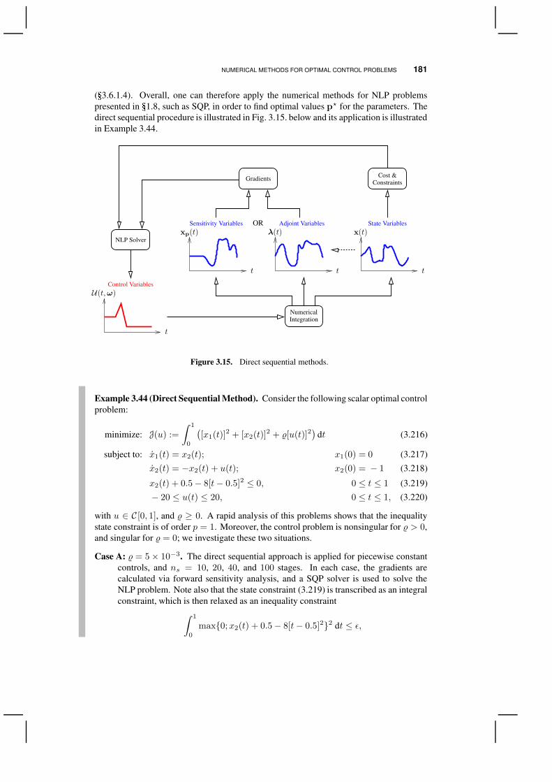
NUMERICAL METHODS FOR OPTIMAL CONTROL PROBLEMS 181
( 3.6.1.4). Overall, one can therefore apply the numerical methods for NLP problemspresented in 1.8, such as SQP, in order to find optimal values p? for the parameters. Thedirect sequential procedure is illustrated in Fig. 3.15. below and its application is illustratedin Example 3.44.
OR
PSfrag replacements
t
t tt
U(t,ω)
x(t)λ(t)xp(t)NLP Solver
(Param. p)
Gradients
NumericalIntegration
Cost &Constraints
Control Variables
State VariablesSensitivity Variables Adjoint Variables
Figure 3.15. Direct sequential methods.
Example 3.44 (Direct Sequential Method). Consider the following scalar optimal controlproblem:
minimize: J(u) :=
∫ 1
0
(
[x1(t)]2 + [x2(t)]
2 + %[u(t)]2)
dt (3.216)
subject to: x1(t) = x2(t); x1(0) = 0 (3.217)x2(t) = −x2(t) + u(t); x2(0) = − 1 (3.218)
x2(t) + 0.5− 8[t− 0.5]2 ≤ 0, 0 ≤ t ≤ 1 (3.219)− 20 ≤ u(t) ≤ 20, 0 ≤ t ≤ 1, (3.220)
with u ∈ C [0, 1], and % ≥ 0. A rapid analysis of this problems shows that the inequalitystate constraint is of order p = 1. Moreover, the control problem is nonsingular for % > 0,and singular for % = 0; we investigate these two situations.
Case A: % = 5× 10⁻³. The direct sequential approach is applied for piecewise constantcontrols, and ns = 10, 20, 40, and 100 stages. In each case, the gradients arecalculated via forward sensitivity analysis, and a SQP solver is used to solve theNLP problem. Note also that the state constraint (3.219) is transcribed as an integralconstraint, which is then relaxed as an inequality constraint
∫ 1
0
max0;x2(t) + 0.5− 8[t− 0.5]22 dt ≤ ε,

182 OPTIMAL CONTROL
with ε = 10−6.
The results of the direct sequential approach are presented in Fig. 3.16., with theoptimal piecewise controls u? and the optimal response x?2 shown on the left andright plots, respectively. The corresponding optimal cost values are reported thefollowing table:
ns 10 20 40 100
J(u?) 1.79751 × 10⁻¹ 1.71482 × 10⁻¹ 1.69614 × 10⁻¹ 1.69161 × 10⁻¹
Observe that the reduction in the optimal cost value is negligible when ns ≥ 40stages; this behavior is in fact typical of control parameterization methods. However,by refining the control profile, one can obtain a better idea of the sequence of con-strained/unconstrained arcs within the optimal solution. While it is unclear whicharcs compose the solution for ns = 10, it becomes obvious, e.g., for ns = 100,that we have three arcs: the first and third arcs are (nonsingular) interior arcs; andthe second arc is a boundary arc for the state inequality constraint. Furthermore,the optimal control appears to be continuous at both the entry and exit times of theboundary arc. To confirm it, a possibility would be to apply the indirect shootingmethod ( 3.6.2.1), by using the present results as initial guess, and check whether allthe necessary conditions of optimality are satisfied.
Case B: % = 0. The results of the direct sequential approach, obtained with the same as-sumptions as in case A, are presented in Fig. 3.16.. The corresponding optimal costvalues are reported the following table:
ns 10 20 40 100
J(u?) 1.13080 × 10⁻¹ 0.97320 × 10⁻¹ 0.96942 × 10⁻¹ 0.96893 × 10⁻¹
Similar to case A, the improvement of the optimal cost value becomes marginalfor ns ≥ 40. (The optimal cost values are lower here since the control is no longerpenalized in the cost functional.) Interestingly, the optimal solution is now composedof four arcs. By inspection, it is not hard to see that: the first arc is a boundary arcfor the control constraint u(t) ≤ 20; the second and fourth arcs are interior arcs; andthe third arc is a boundary arc for the state inequality constraint. Regarding interiorarcs in particular, we have:
0 =Hu = λ2(t)
0 =ddtHu = λ2(t) = −2x2(t)− λ1(t) + λ2(t)
0 =d2
dt2Hu = −2x2(t)− λ1(t) + λ2(t) = −2[u(t)− x2(t)]− 2x1(t)
Hence, both interior arcs are singular arcs of order p = 1, and u?(t) = x?2(t)−x?1(t)along these arcs. Moreover, the optimal control appears to be discontinuous at thefunction between boundary and interior arcs. Again, it would be interesting to confirmthese results upon application of an indirect shooting method ( 3.6.2.1).
Since the ODEs are solved at each iteration of the NLP solver, direct sequential methodsare often called feasible path methods. These methods are known to be very robust as

NUMERICAL METHODS FOR OPTIMAL CONTROL PROBLEMS 183
-4
-2
0
2
4
6
8
10
12
14
0 0.2 0.4 0.6 0.8 1
PSfrag replacements
t
u?(t)u?(t
)
x?2(t)x2(t) + 0.5− 8[t− 0.5]2 = 0
Optimal Results for ns = 10 Stages
Optimal Results for ns = 20 StagesOptimal Results for ns = 40 Stages
Optimal Results for ns = 100 Stages-1
-0.5
0
0.5
1
1.5
0 0.2 0.4 0.6 0.8 1
PSfrag replacements
t
u?(t)
x?2(t)
x? 2(t
)
x2(t) + 0.5− 8[t− 0.5]2 = 0
Optimal Results for ns = 10 Stages
Optimal Results for ns = 20 StagesOptimal Results for ns = 40 Stages
Optimal Results for ns = 100 Stages
-4
-2
0
2
4
6
8
10
12
14
0 0.2 0.4 0.6 0.8 1
PSfrag replacements
t
u?(t)
u?(t
)
x?2(t)x2(t) + 0.5− 8[t− 0.5]2 = 0
Optimal Results for ns = 10 Stages
Optimal Results for ns = 20 Stages
Optimal Results for ns = 40 StagesOptimal Results for ns = 100 Stages
-1
-0.5
0
0.5
1
1.5
0 0.2 0.4 0.6 0.8 1
PSfrag replacements
t
u?(t)
x?2(t)
x? 2(t
)
x2(t) + 0.5− 8[t− 0.5]2 = 0
Optimal Results for ns = 10 Stages
Optimal Results for ns = 20 Stages
Optimal Results for ns = 40 StagesOptimal Results for ns = 100 Stages
-4
-2
0
2
4
6
8
10
12
14
0 0.2 0.4 0.6 0.8 1
PSfrag replacements
t
u?(t)
u?(t
)
x?2(t)x2(t) + 0.5− 8[t− 0.5]2 = 0
Optimal Results for ns = 10 StagesOptimal Results for ns = 20 Stages
Optimal Results for ns = 40 Stages
Optimal Results for ns = 100 Stages-1
-0.5
0
0.5
1
1.5
0 0.2 0.4 0.6 0.8 1
PSfrag replacements
t
u?(t)
x?2(t)
x? 2(t
)
x2(t) + 0.5− 8[t− 0.5]2 = 0
Optimal Results for ns = 10 StagesOptimal Results for ns = 20 Stages
Optimal Results for ns = 40 Stages
Optimal Results for ns = 100 Stages
-4
-2
0
2
4
6
8
10
12
14
0 0.2 0.4 0.6 0.8 1
PSfrag replacements
t
u?(t)
u?(t
)
x?2(t)x2(t) + 0.5− 8[t− 0.5]2 = 0
Optimal Results for ns = 10 StagesOptimal Results for ns = 20 StagesOptimal Results for ns = 40 Stages
Optimal Results for ns = 100 Stages
-1
-0.5
0
0.5
1
1.5
0 0.2 0.4 0.6 0.8 1
PSfrag replacements
t
u?(t)
x?2(t)
x? 2(t
)
x2(t) + 0.5− 8[t− 0.5]2 = 0
Optimal Results for ns = 10 StagesOptimal Results for ns = 20 StagesOptimal Results for ns = 40 Stages
Optimal Results for ns = 100 Stages
Figure 3.16. Results of the direct sequential approach as applied to Example 3.44 with % = 5×10⁻³
(case A), for ns = 10, 20, 40, and 100. Left plots: optimal piecewise control u?; right plots: optimalresponse x2
?
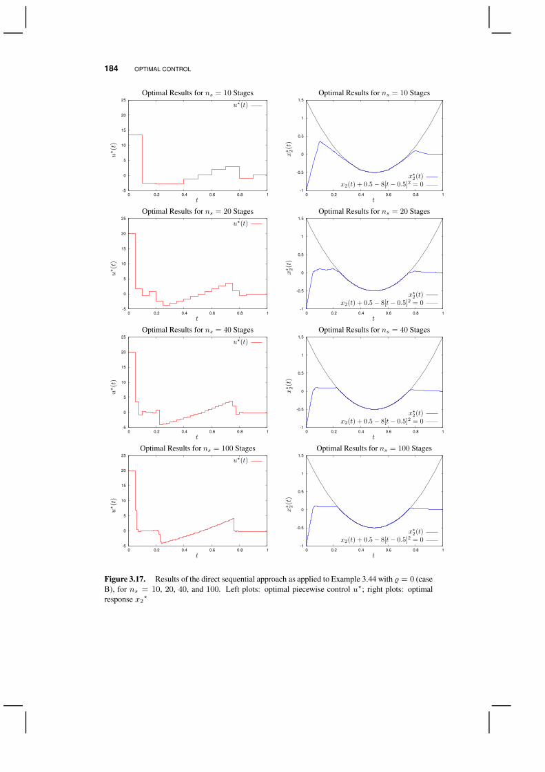
184 OPTIMAL CONTROL
-5
0
5
10
15
20
25
0 0.2 0.4 0.6 0.8 1
PSfrag replacements
t
u?(t)u?(t
)
x?2(t)x2(t) + 0.5− 8[t− 0.5]2 = 0
Optimal Results for ns = 10 Stages
Optimal Results for ns = 20 StagesOptimal Results for ns = 40 Stages
Optimal Results for ns = 100 Stages-1
-0.5
0
0.5
1
1.5
0 0.2 0.4 0.6 0.8 1
PSfrag replacements
t
u?(t)
x?2(t)
x? 2(t
)
x2(t) + 0.5− 8[t− 0.5]2 = 0
Optimal Results for ns = 10 Stages
Optimal Results for ns = 20 StagesOptimal Results for ns = 40 Stages
Optimal Results for ns = 100 Stages
-5
0
5
10
15
20
25
0 0.2 0.4 0.6 0.8 1
PSfrag replacements
t
u?(t)
u?(t
)
x?2(t)x2(t) + 0.5− 8[t− 0.5]2 = 0
Optimal Results for ns = 10 Stages
Optimal Results for ns = 20 Stages
Optimal Results for ns = 40 StagesOptimal Results for ns = 100 Stages
-1
-0.5
0
0.5
1
1.5
0 0.2 0.4 0.6 0.8 1
PSfrag replacements
t
u?(t)
x?2(t)x? 2(t
)
x2(t) + 0.5− 8[t− 0.5]2 = 0
Optimal Results for ns = 10 Stages
Optimal Results for ns = 20 Stages
Optimal Results for ns = 40 StagesOptimal Results for ns = 100 Stages
-5
0
5
10
15
20
25
0 0.2 0.4 0.6 0.8 1
PSfrag replacements
t
u?(t)
u?(t
)
x?2(t)x2(t) + 0.5− 8[t− 0.5]2 = 0
Optimal Results for ns = 10 StagesOptimal Results for ns = 20 Stages
Optimal Results for ns = 40 Stages
Optimal Results for ns = 100 Stages-1
-0.5
0
0.5
1
1.5
0 0.2 0.4 0.6 0.8 1
PSfrag replacements
t
u?(t)
x?2(t)
x? 2(t
)
x2(t) + 0.5− 8[t− 0.5]2 = 0
Optimal Results for ns = 10 StagesOptimal Results for ns = 20 Stages
Optimal Results for ns = 40 Stages
Optimal Results for ns = 100 Stages
-5
0
5
10
15
20
25
0 0.2 0.4 0.6 0.8 1
PSfrag replacements
t
u?(t)
u?(t
)
x?2(t)x2(t) + 0.5− 8[t− 0.5]2 = 0
Optimal Results for ns = 10 StagesOptimal Results for ns = 20 StagesOptimal Results for ns = 40 Stages
Optimal Results for ns = 100 Stages
-1
-0.5
0
0.5
1
1.5
0 0.2 0.4 0.6 0.8 1
PSfrag replacements
t
u?(t)
x?2(t)
x? 2(t
)
x2(t) + 0.5− 8[t− 0.5]2 = 0
Optimal Results for ns = 10 StagesOptimal Results for ns = 20 StagesOptimal Results for ns = 40 Stages
Optimal Results for ns = 100 Stages
Figure 3.17. Results of the direct sequential approach as applied to Example 3.44 with % = 0 (caseB), for ns = 10, 20, 40, and 100. Left plots: optimal piecewise control u?; right plots: optimalresponse x2
?
NUMERICAL METHODS FOR OPTIMAL CONTROL PROBLEMS 185
long as the dynamic system is stable in the control/parameter range of interest. Moreover,they guarantee the accuracy of the state variables through the error control mechanismof the numerical integration solvers. However, finding an optimal, or even a feasiblesolution, may prove difficult when the system is unstable or the response is undefined forcertain control/parameter values. In addition, much computational effort may be wastedin obtaining accurate state values when the controls/parameters are far from their optimalvalues. These considerations motivate the direct simultaneous methods which are presentedin the following subsection.
3.6.3.2 Direct Simultaneous Methods In direct simultaneous methods, the originaloptimal control problem (3.201–3.206)is transcribed into a finite dimensional NLP problemthrough the discretization of all the variables, i.e., both the control and the state variables.Accordingly, this approach is often referred to as full discretization in the literature.
Regarding the control variables first, similar parameterizations as those described in thedirect sequential approach (3.6.3.1) can be used; for the jth control variable in the controlstage k, we have
uj(t) = Ukj (t,ωk) =
N∑
i=0
ωki,jφ(M)i (
t−tk−1
tk−tk−1), tk−1 ≤ t ≤ tk,
with φ(M)i (·) given by (3.208). In particular, piecewise constant or piecewise linear control
parameterizations are often considered in practical applications.To approximate the state variables, on the other hand, a family of polynomials is also
considered on each interval, so that
x(t) = Xk(t, ξk), tk−1 ≤ t ≤ tk, k = 1, . . . , ns,
with ξk ∈ IRnkξ . For simplicity, we shall assume subsequently that the polynomials have the
same order N for each state variable and each stage. Different polynomial representationshave been suggested in the literature:
Lagrange Polynomials [35]: Similar to the control parameterization, the jth statevariable in stage k is calculated as
xj(t) = X kj (t, ξk) =
N∑
i=0
ξki,jφ(N)i (
t−tk−1
tk−tk−1), tk−1 ≤ t ≤ tk, (3.221)
with φ(N)i (·) given by (3.208).
Monomial Basis Representation [4]: The jth state variable in stage k is calculated as
xj(t) = X kj (t, ξk) = ξk0,j + (tk − tk−1)N∑
i=1
ξki,jΩ(N)i ( t−tk−1
tk−tk−1), tk−1 ≤ t ≤ tk,
(3.222)
where Ω(N)i (·) is a polynomial of order N satisfying
Ω(N)i (0) := 0
ddt
Ω(N)i (τq) := δi,q , q = 1, . . . , N,

186 OPTIMAL CONTROL
with collocation points 0 = τ0 ≤ τ1 < τ2 < · · · < τN ≤ 1.
By using either of the foregoing polynomial representations, the problem (3.201–3.206)can be rewritten into the following form:
minimize:ns∑
k=1
∫ tk
tk−1
`(t,X k(t, ξk),Uk(t,ωk),v) dt+ φ(X ns(tns , ξns),v) (3.223)
subject to: Xkt (tk,q , ξ
k) = f(tk,q ,Xk(tk,q , ξ
k),Uk(tk,q ,ωk),v) (3.224)
X1(t0, ξ
1) = h(v); Xk(tk, ξ
k) = Xk−1(tk , ξ
k−1) (3.225)ψ(Xns(tns , ξ
ns),v) = 0 (3.226)κ(Xns(tns , ξ
ns),v) ≤ 0 (3.227)
g(tk,q ,Xk(tk,q , ξ
k),Uk(tk,q ,ωk),v) ≤ 0 (3.228)
ξk ∈ [ξL, ξU ], ω ∈ [ωL,ωU ], v ∈ [vL,vU ], (3.229)
where tk,q := tk−1 + τq(tk − tk−1), with k = 1, . . . , ns, and q = 1, . . . , N .A number of remarks are in order:
The continuous differential equations (3.202) are discretized into (N + 1) equalityconstraints (3.224) in each time stage, k = 1, . . . , ns; moreover, the conditions(3.225) are imposed so that the state variables are continuous at the junctions betweenconsecutive time stages. That is, a common characteristic of direct simultaneousmethods is that the differential equations are, in general, satisfied at the solutionof the optimization problem only; for this reason, these methods are often calledinfeasible path methods.
The inequality state constraints (3.205) are also discretized into a finite number ofinequality constraints (3.228), which must hold at every collocation point in eachtime stage. Hence, an advantage of simultaneous methods over sequential methodsis that they allow handling state inequality constraints more easily, i.e., by enforcinginterior-point inequality constraint at collocation points.
The time stages t1, . . . , tns can be optimized very easily in direct simultaneous meth-ods, together with the other parameters (ξ1, . . . , ξns ,ω1, . . . ,ωns ,v).
Unlike sequential methods, direct simultaneous methods have the advantage of not wast-ing computational effort in obtaining feasible solutions to the ODEs, away from the solutionof the optimization problem. This also allows to handle efficiently those dynamic systemsfor which instabilities occur in the range of inputs, or for which a solution does not existfor certain inputs. On the other hand, however, only the converged solution satisfies theODEs, while the intermediate solutions have no physical meaning. Moreover, one doesnot know a priori how many time stages and collocation points should be taken for obtain-ing an accurate solution to the ODEs. Finally, the resulting NLP problem in the variables(ξ1, . . . , ξns ,ω1, . . . ,ωns ,v) is a large-scale NLP problem which may be difficult to solve.This difficulty has led to the development of special decomposition techniques to solve suchNLP problems.

NOTES AND REFERENCES 187
3.7 NOTES AND REFERENCES
Only a brief discussion on the problem of existence of an optimal solution has been givenin 3.3. A comprehensive treatment of the existence problem can be found in the bookby Macki and Strauss [38, Chapter 4]. For a more mathematical presentation of existenceresults, the interested reader is referred to the book by Cesari [16].
The seminal textbook for the variational approach presented in 3.4 is the book by Brysonand Ho [12]. The book by Kamien and Schwartz [28] has also been useful in writing thischapter, especially regarding the interpretation of the adjoint variables.
In this chapter, we have also limited our presentation of the sufficient conditions to theso-called Mangasarian conditions. More general sufficient conditions can be found in thesurvey paper by Seierstad and Sydstæter [49]. For local sufficient conditions, we refer theinterested reader to the book by Bryson and Ho [12, Chapter 6].
Regarding 3.5 on maximum principles for optimal control problems, the referencetextbook is that by Pontryagin and coworkers [41]; a proof of the Pontryagin MaximumPrinciple can also be found in [38, Chapter 5]. The indirect adjoining approach for optimalcontrol problems with pure path constraints was originally introduced by Pontryagin [41].For a recent survey on maximum principles for problems having both mixed and pure stateconstraints, see the paper by [25]. A comprehensive discussion of necessary conditions forsingular control problems, including second order necessary conditions, can be found inthe paper by Kelley and coworkers [29].
For a general introduction to numerical methods for initial value problems in ODEsand DAEs see the book by Brenan, Campbell and Petzold [11], or Ascher and Petzold [3].Concerning the calculation of gradients for functionals with ODEs embedded, see, e.g.,[45, 56] for the forward sensitivity approach and [54] for the adjoint sensitivity approach.A detailed discussion of indirect solution methods for optimal control problems, includingthe indirect shooting approach, can be found in [12]. Finally, for more information on directsolution methods, see [54, 56] for the sequential approach and [8, 9] for the simultaneousapproach.