Embed Size (px)
Citation preview

Design of Experiments:
The D-Optimal Approach and Its
Implementation As a Computer Algorithm
Fabian Triefenbach
15th January 2008
Bachelor’s Thesis in Information and Communication Technology
15 ECTS
Supervisor at UmU: Jurgen Borstler
Supervisor at FH-SWF: Thomas Stehling
Examiner: Per Lindstrom
Umea UniversityDepartment of Computing Science
SE-901 87 UMEASWEDEN
South Westphalia University of Applied SciencesDepartment of Engineering and Business Sciences
D-59872 MESCHEDEGERMANY


Abstract
Motivation: The use of experiments in an effective way to analyze and optimize agiven process is a problem statement which should be paid more attention to in theengineering community. Frequently, experiments are first performed and the measureddata is analyzed afterwards. In contrast to this, statistical methods, like the concept ofDesign of Experiments, should be used to plan experimental designs and perform sets ofwell selected experiments to get the most informative combination out of the given fac-tors. Problem Statement: The Swedish company Umetrics AB is developing specialsoftware tools which deal with this field of statistical experimental design. Inside thesoftware MODDE a feature for the creation of a special design type, the D-optimal de-sign, is given. The aim of the present thesis is the reimplementation of this program unitwith improvements in the quality of the generated designs and the computational ef-fort. Approach: D-optimal designs are based on a computer-aided exchange procedurewhich creates the optimal set of experiments. An intensive literature study brings forthsix different approaches to handle this exchange with a computer algorithm. In detail acomparison and evaluation of the Fedorov procedure, the modified Fedorov procedure,the DETMAX algorithm, the k-exchange algorithm, and the kl-exchange algorithm isperformed. Based on this, a new algorithm, the modified kl-exchange algorithm, is devel-oped and used for the implementation in C++. Results: The outcome of the presentthesis is an implementation of the four most advisable algorithms. The Fedorov andnormal Fedorov algorithm generate the best designs considering the D-optimality of thedesigns but are very time-consuming for big data sets. As an alternative the k-exchangealgorithm and a modified version of the kl-exchange algorithm are implemented to cre-ate comparable designs with a much higher computational efficiency. Conclusion: Thenew implementation of the D-optimal process creates designs which are at least com-parable to the old approach considering the quality or D-optimality of the designs. Inaddition to this, the computational efficiency, especially regarding big data sets with10 and more factors, is higher. The selection of the adequate algorithm for the givenproblem formulation has to be performed by the user. As a future work, this processshould be carried out to an automatic procedure based on a complexity analysis of thefour implemented alternatives.
keywords: D-Optimal Designs, Design of Experiments, Exchange Algorithms, (Mod-ified) Fedorov Algorithm, k-Exchange Algorithm, (Modified) kl-Exchange Algorithm,Mitchell’s DETMAX Algorithm, Bayesian Modification, Inclusions, Mixture Designs,Sequential Start Design, Qualitative Factors.


Acknowledgement
Overall, I would like to thank my German institute, the South Westphalia University ofApplied Science in Meschede, and my host university in Sweden, the Umea University,for making this thesis possible. Especially my both supervisors, Prof. Borstler andProf. Stehling, helped to arrange an agreement and gave me the chance to write mythesis abroad. With reference to the received assistance during my thesis, I appreciatethe encouragement of both supervisors. In addition to this, I would like to thank myexaminer Per Lindstrom.
The second group of people I would like to give thanks to is the whole staff of thecompany Umetrics AB. My advisors, Ake Nordahl and Joakim Sundstrom, have alwaysbeen great contact persons and were obliging in any situation. Also the other staffmembers helped me with advices and at least improved my Swedish skills. Therefore, Iwould like to thank Jonas, Conny, Erik, Lennart, Anders, Jerker and all the rest of thepersonnel at the Umea headquarter. Special thanks are targeted at Ing-Marie Olssonfor her previous work and the backup during the development process. Tack ska ni ha.


Dedication
I dedicate this thesis to my family and my girlfriend Christina, who gave me such astrong support during the whole development process. Thank you.


Contents
1 Introduction 11.1 Thesis Outline . . . . . . . . . . . . . . . . . . . . . . . . . . . . . . . . 11.2 Design of Experiments . . . . . . . . . . . . . . . . . . . . . . . . . . . . 2
1.2.1 Preface . . . . . . . . . . . . . . . . . . . . . . . . . . . . . . . . 21.2.2 Experiments . . . . . . . . . . . . . . . . . . . . . . . . . . . . . 21.2.3 Factors & Responses . . . . . . . . . . . . . . . . . . . . . . . . . 21.2.4 Basic Principles of DoE . . . . . . . . . . . . . . . . . . . . . . . 41.2.5 Model Concept . . . . . . . . . . . . . . . . . . . . . . . . . . . . 41.2.6 Experimental Objectives . . . . . . . . . . . . . . . . . . . . . . . 5
1.3 Experimental Designs . . . . . . . . . . . . . . . . . . . . . . . . . . . . 71.3.1 Statistical Designs . . . . . . . . . . . . . . . . . . . . . . . . . . 71.3.2 General Notation . . . . . . . . . . . . . . . . . . . . . . . . . . . 8
1.4 MODDE 8 and Umetrics AB . . . . . . . . . . . . . . . . . . . . . . . . 81.4.1 Umetrics AB, Umea . . . . . . . . . . . . . . . . . . . . . . . . . 81.4.2 MODDE Version 8.0 . . . . . . . . . . . . . . . . . . . . . . . . . 9
2 D-Optimal Designs 102.1 The Need for D-Optimal Designs . . . . . . . . . . . . . . . . . . . . . . 10
2.1.1 Irregular Experimental Regions . . . . . . . . . . . . . . . . . . . 102.1.2 Inclusion of Already Performed Experiments . . . . . . . . . . . 112.1.3 The Use of Qualitative Factors . . . . . . . . . . . . . . . . . . . 112.1.4 Reducing the Number of Experiments . . . . . . . . . . . . . . . 122.1.5 Fitting of Special Regression Models . . . . . . . . . . . . . . . . 13
2.2 The D-Optimal Approach . . . . . . . . . . . . . . . . . . . . . . . . . . 132.2.1 Candidate Set . . . . . . . . . . . . . . . . . . . . . . . . . . . . 132.2.2 Design Matrix . . . . . . . . . . . . . . . . . . . . . . . . . . . . 132.2.3 Information and Dispersion Matrix . . . . . . . . . . . . . . . . . 14
2.3 Criteria for the Best D-Optimal Design . . . . . . . . . . . . . . . . . . 142.4 A Basic Example . . . . . . . . . . . . . . . . . . . . . . . . . . . . . . . 162.5 Fitting the Model . . . . . . . . . . . . . . . . . . . . . . . . . . . . . . . 182.6 Scaling . . . . . . . . . . . . . . . . . . . . . . . . . . . . . . . . . . . . . 19
vii
viii CONTENTS
2.7 Number of Design Runs . . . . . . . . . . . . . . . . . . . . . . . . . . . 202.8 Bayesian Modification . . . . . . . . . . . . . . . . . . . . . . . . . . . . 20
2.8.1 The Addition of Potential Terms . . . . . . . . . . . . . . . . . . 202.8.2 Scaling the Factors . . . . . . . . . . . . . . . . . . . . . . . . . . 212.8.3 Bayesian Example . . . . . . . . . . . . . . . . . . . . . . . . . . 22
3 D-Optimal Designs as a Computer Algorithm 243.1 Exchange Algorithms . . . . . . . . . . . . . . . . . . . . . . . . . . . . . 24
3.1.1 General Exchange Procedure . . . . . . . . . . . . . . . . . . . . 253.1.2 DETMAX Algorithm . . . . . . . . . . . . . . . . . . . . . . . . 253.1.3 Fedorov Algorithm . . . . . . . . . . . . . . . . . . . . . . . . . . 273.1.4 Modified Fedorov Algorithm . . . . . . . . . . . . . . . . . . . . . 283.1.5 k-Exchange Algorithm . . . . . . . . . . . . . . . . . . . . . . . . 293.1.6 kl-Exchange Algorithm . . . . . . . . . . . . . . . . . . . . . . . 303.1.7 Modified kl-Exchange Algorithm . . . . . . . . . . . . . . . . . . 32
3.2 Generation of the Start Design . . . . . . . . . . . . . . . . . . . . . . . 323.3 Comparison of Exchange Algorithms . . . . . . . . . . . . . . . . . . . . 34
4 The Implementation in C++ 374.1 Purpose & Goal . . . . . . . . . . . . . . . . . . . . . . . . . . . . . . . . 37
4.1.1 Current Implementation . . . . . . . . . . . . . . . . . . . . . . . 374.1.2 Task & Goal . . . . . . . . . . . . . . . . . . . . . . . . . . . . . 374.1.3 Preliminaries for a Reimplementation . . . . . . . . . . . . . . . 38
4.2 Final Implementation . . . . . . . . . . . . . . . . . . . . . . . . . . . . 384.2.1 Input & Output . . . . . . . . . . . . . . . . . . . . . . . . . . . 384.2.2 Integration & Program Flow . . . . . . . . . . . . . . . . . . . . 414.2.3 Variables . . . . . . . . . . . . . . . . . . . . . . . . . . . . . . . 434.2.4 Exchange Algorithms . . . . . . . . . . . . . . . . . . . . . . . . 454.2.5 Features . . . . . . . . . . . . . . . . . . . . . . . . . . . . . . . . 50
5 Summary & Conclusions 575.1 Summary . . . . . . . . . . . . . . . . . . . . . . . . . . . . . . . . . . . 575.2 Conclusions . . . . . . . . . . . . . . . . . . . . . . . . . . . . . . . . . . 585.3 Limitations . . . . . . . . . . . . . . . . . . . . . . . . . . . . . . . . . . 595.4 Future Work . . . . . . . . . . . . . . . . . . . . . . . . . . . . . . . . . 59
Refrences 60
Nomenclature 62
A Source Code 65

List of Figures
1.1 Factors & Responses . . . . . . . . . . . . . . . . . . . . . . . . . . . . . 31.2 COST Approach & DoE . . . . . . . . . . . . . . . . . . . . . . . . . . . 41.3 Symmetrical Distribution of Experiments . . . . . . . . . . . . . . . . . 51.4 Experimental Objectives . . . . . . . . . . . . . . . . . . . . . . . . . . . 61.5 Comparison of Statistical Designs . . . . . . . . . . . . . . . . . . . . . . 7
2.1 Examples for Irregular Experimental Regions . . . . . . . . . . . . . . . 112.2 Design With Multi-Level Qualitative Factors . . . . . . . . . . . . . . . 122.3 Distribution of the Candidate Set . . . . . . . . . . . . . . . . . . . . . . 172.4 Distribution of the Design Matrix . . . . . . . . . . . . . . . . . . . . . . 172.5 Rule of Sarrus for the Calculation of a Determinant . . . . . . . . . . . 182.6 Distribution of Normal and Bayesian Design Matrix . . . . . . . . . . . 22
3.1 Flow Chart of the D-Optimal Process . . . . . . . . . . . . . . . . . . . 24
4.1 Screenshot: MODDE Design Wizard — Factor Definition . . . . . . . . 394.2 Screenshot: MODDE Design Wizard — D-Optimal Specification . . . . 404.3 Screenshot: MODDE Design Wizard — Evaluation Page . . . . . . . . . 414.4 Screenshot: MODDE Worksheet . . . . . . . . . . . . . . . . . . . . . . 414.5 Program Flow I . . . . . . . . . . . . . . . . . . . . . . . . . . . . . . . . 424.6 Program Flow II . . . . . . . . . . . . . . . . . . . . . . . . . . . . . . . 434.7 Layout of the Extended Model Matrix . . . . . . . . . . . . . . . . . . . 444.8 Use of Indices to Calculate the Delta-Matrix . . . . . . . . . . . . . . . . 504.9 Layout of the Candidate Set . . . . . . . . . . . . . . . . . . . . . . . . . 514.10 Layout of the Sequential Start Design . . . . . . . . . . . . . . . . . . . 54
ix

x LIST OF FIGURES

List of Tables
1.1 22 Full Factorial Design . . . . . . . . . . . . . . . . . . . . . . . . . . . 8
2.1 Minimum Number of Design Runs for Screening Designs . . . . . . . . . 122.2 Candidate Set for Two Factors with Three Levels . . . . . . . . . . . . . 162.3 Determinants of Different Designs . . . . . . . . . . . . . . . . . . . . . 18
3.1 Comparison of Different Algorithms . . . . . . . . . . . . . . . . . . . . 343.2 Comparison of Different Algorithms (Bayesian Modification) . . . . . . . 36
4.1 List of Variables . . . . . . . . . . . . . . . . . . . . . . . . . . . . . . . 444.2 List of Potential Terms . . . . . . . . . . . . . . . . . . . . . . . . . . . . 524.3 Columns Needed to Handle Qualitative Factors . . . . . . . . . . . . . . 55
5.1 Comparison of the Old and New Implementation . . . . . . . . . . . . . 58
xi

xii LIST OF TABLES

List of Algorithms
3.1 DETMAX algorithm by Mitchell (1974) . . . . . . . . . . . . . . . . . . . 263.2 Fedorov Algorithm (1972) . . . . . . . . . . . . . . . . . . . . . . . . . . . 283.3 Modified Fedorov Algorithm by Cook & Nachtsheim (1980) . . . . . . . . 293.4 k-Exchange Algorithm by Johnson & Nachtsheim (1983) . . . . . . . . . 303.5 kl-Exchange Algorithm by Atkinson & Donev (1989) . . . . . . . . . . . 313.6 Modified kl-Exchange Algorithm . . . . . . . . . . . . . . . . . . . . . . . 33
xiii

xiv LIST OF ALGORITHMS

List of C++ Listings
4.1 Fedorov Algorithm . . . . . . . . . . . . . . . . . . . . . . . . . . . . . . 454.2 Modified Fedorov Algorithm . . . . . . . . . . . . . . . . . . . . . . . . . 464.3 k-Exchange Algorithm . . . . . . . . . . . . . . . . . . . . . . . . . . . . 464.4 Modified kl-Exchange Algorithm . . . . . . . . . . . . . . . . . . . . . . 484.5 Function: calculateDeltaMatrix() . . . . . . . . . . . . . . . . . . . . . . 494.6 Function: doBayesianScaling() . . . . . . . . . . . . . . . . . . . . . . . 524.7 Function: createQ() . . . . . . . . . . . . . . . . . . . . . . . . . . . . . 534.8 Function: exchangePoints( int xi, int xj, bool bdublicates) . . . . . . . . 53
xv

xvi LIST OF C++ LISTINGS

Chapter 1
Introduction
1.1 Thesis Outline
The present thesis depicts the development process of a C++ computer algorithm togenerate D-optimal designs in the field of Design of Experiments (DoE).
The report starts with the description of the basic principles of DoE and explainsthe elementary methods and definitions used in this field. In general, DoE is a conceptthat uses a desired set of experiments to optimize or investigate a studied object. Afterthis brief overview about the concept, a special design type, the D-optimal design isexamined in the following chapter. D-Optimality characterizes the selection of a specialset of experiments which fulfills a given criterion. From the ground up, the whole conceptof D-optimal designs and their application is shown. Starting with the algebraic andgeometric approach, more statistical and methodical details are illustrated afterwards.
The generation of the D-optimal design is accomplished by the use of an exchangealgorithm. Chapter 3 of this report contains a review and comparison of existing algo-rithms which are presented in diverse publications. The comparison considers Mitchell’s(1974) DETMAX algorithm, the Fedorov (1972) procedure, the modified Fedorov pro-cedure by Cook & Nachtsheim (1980), the k-exchange by Johnson & Nachtsheim (1983)and the kl-exchange algorithm (Atkinson & Donev 1989). In addition to this, a modifiedversion of the kl-exchange is developed and included in the investigation. The algorithmsare explained in detail and evaluated depending on the computational efficiency and thequality of the generated designs. In order to make the created designs independent onan assumed model, a Bayesian modification of the process is introduced and exemplifiedin chapter 2.
Chapter 4 gives detailed information about the implementation of the D-optimalselection process. The work described in this chapter is done at the Umetrics ABoffice in Umea, Sweden, and will be implemented in a future release of the MODDEsoftware. Starting with an explicitly definition of the requirements, the program flowand integration of the new source code is explained. After this, a description of the fourimplemented algorithm is given and clarified with extracts from the C++ source code.The chapter ends with a description of the main features of the implementation andexplains the realization in more detail.
The thesis ends with a summary of the work and analyses the achievements made bythe final implementation with a conclusion. After this discusion of the result, a prospectof the future work based on the present thesis is given.
1

2 Chapter 1. Introduction
1.2 Design of Experiments
1.2.1 Preface
Experiments are used in nearly every area to solve problems in an effective way. Theseexperimentations can be found both in daily life and in advanced scientific areas. A pre-sentable example for an ordinary experiment is the baking of a cake, where the selectionand the amount of the ingredients influence the taste. In this basic example, the ingre-dients are flour, butter, eggs, sugar and baking powder. The aim of the experimenteris to create the cake with the best taste. A possible outcome of the first baking processis a cake that is too dry. As a result, the experimenter reduces the amount of flour orenhances the amount of butter. In order to bake the best cake, the recipe should bechanged for every new cake. As a result of this process, we get a set of different recipeswhich lead to different tasting cakes.
Similar observations are used in the scientific area to find significant informationabout a studied object. An object can be, e.g., a chemical mixture, a mechanicalcomponent or every other product. A good example in this field is the development of aspecial oil which has to be observed under different conditions, like high pressure or lowtemperature. Finding the optimal mixture which has the best performance in differentsituations, is one of the most important stages during such a development process.
1.2.2 Experiments
In general, an experiment is an observation which leads to characteristic informationabout a studied object. The classical purpose for such an observation is a hypothesisthat has to be veryfied or falsified with an investigation. In this classical approach, theexperimental setup is chosen for the specified problem statement and the experimentertests if the hypothesis is true or false (Trochim 2006).
In the present thesis, we deal with another use of experiments. With the con-cept of Design of Experiments (DoE) we use a set of well selected experiments whichhas to be performed by the experimenter. The aim of this so-called design is to op-timize a process or system by performing each experiment and to draw conclusionsabout the significant behavior of the studied object from the results of the experi-ments. The examples in the preface follow this basic idea and show two useful situ-ations where DoE is applicable. Considering the costs for a single experiment, mini-mizing the amount of performed experiments is always an aim. With DoE, this num-ber is kept as low as possible and the most informative combination of the factorsis chosen (Eriksson et al. 2000). Hence, DoE is an effective and economical solution.
The term experiment is used in DoE even if we do not have a hypothesis to test. Toavoid misunderstandings, we strictly have to differentiate between the notation of DoEand normal experimental design. The following section of this introduction deals withthe general approach of DoE and gives definitions used in the field.
1.2.3 Factors & Responses
We always have two types of variables when we perform experiments in the field ofDoE, responses and factors. The response gives us information about the investigatedsystem, and the factors are used to manipulate it. Normal factors can be set to two or

1.2. Design of Experiments 3
more values and have a defined range. The factors can be divided into three groups,depending on different criteria.
Figure 1.1: Factors & Responses: A process or a system can be manipulated by one ormore different input factors. These modifications takes effect on the responses and canbe measured.
Controllable & Uncontrollable Factors
One way to differentiate factors is to divide them into controllable and uncontrollablefactors. The controllable factors are normal process factors that are easy to monitorand investigate. The experimenter can observe them and has the opportunity to changethem. By contrast, an uncontrolled factor is hard to regulate because it is mostly adisturbance value or an external influence. Uncontrolled factors can have a high im-pact on the response and therefore should always be considered during the experiments(Eriksson et al. 2000, Wu & Hamada 2000). A good example of a controlled factoris the temperature inside a closed test arrangement. In contrast to this, the outsidetemperature is an example of an uncontrolled factor which can not be influenced.
Quantitative & Qualitative Factors
Another method to categorize factors in the broader sense is to distinguish betweenquantitative and qualitative factors. The values of a quantitative factor have a givenrange and a continuous scale, whereas qualitative factors have only distinct values (Wu& Hamada 2000, Montgomery 1991). To use the earlier example, the temperature canbe seen as a quantitative value. An example of a qualitative factor is the differentiationbetween variant types of oil, developed by different suppliers.
Process & Mixture Factors
The third group consists of process and mixture factors. Process factors can be changedindependently and do not influence each other. They are normally expressed by anamount or level and can be seen as regular factors. Mixture factors stand for theamounts of ingredients in a mixture. They all are part of a formulation and add up toa value of 100%. A mixture factor cannot be changed independently, so special designsare needed to deal with this type of factors (Eriksson et al. 2000, Montgomery 1991).
Responses
As described above, a response is the general condition of a studied system during thechange of the factors. It is possible and often useful to measure multiple responsesthat react differently on the factor adjustments. A response can either be a continuous

4 Chapter 1. Introduction
or a discrete value (Wu & Hamada 2000). A discrete scale, e.g., can be an ordinalmeasurement with three values (good, OK, bad). These values are hard to process, soit is always recommended to use a continuous scale if possible.
1.2.4 Basic Principles of DoE
To understand the basic idea of DoE, we should first examine how experimental designwas done traditionally. As Eriksson et al. (2000, p. 2) describe, the intuitive approachis to ‘chang[e] the value of one separate factor at a time until no further improvementis accomplished’. Figure 1.2 illustrates how difficult finding the optimum can be withthis co-called COST approach (Change Only one Separate factor at a Time). Theexperimenter does not know at which value the changing of the factor x1 should bestopped because a further improvement can not be observed. But the exact value isvery important considering it in combination with the later adjusted factor x2.
Figure 1.2: COST Approach & DoE, based on Eriksson et al. (2000, p. 3, fig. 0.1):Changing all factors simultaneously, as shown in the lower right corner, gives betterinformation about the optimum than the COST approach where all factors are changedsuccessively.
The given situation from figure 1.2 can also be investigated with the use of DoE.In this case, we create a special set of experiments around a so-called center-point. Asshown in the lower right corner of the diagram, we use a uniform set of experimentswhich allows obtaining a direction for a better result. These basic examples clearlyshow the advantages of changing all relevant factors at the same time and consequentlyshow the importance of DoE (Wu & Hamada 2000, Eriksson et al. 2000).
As shown above, the basic concept of DoE is to arrange a symmetrical distributionof experiments around a center-point. With a given range for all input factors, thecalculation of this point is easy. Figure 1.3 shows a simple example with the factorsx1 (200 to 400), x2 (50 to 100) and x3 (50 to 100). The calculated center-point in themiddle of the cubic pattern has the coordinates 300/75/75.
1.2.5 Model Concept
The base for DoE is an approximation of reality with the help of a mathematical model.The important aspects of the investigated system are represented by the use of fac-

1.2. Design of Experiments 5
Figure 1.3: Symmetrical Distribution of Experiments, based on Eriksson et al. (2000,p. 8, fig. 1.1): The three factors x1, x2 and x3 are, depending on their range, ordered ina cubic pattern around the center-point experiment (standard).
tors and responses. A model is never 100% right, but simply helps to transport thecomplexity of the reality into an equation which is easy to handle (Eriksson et al. 2000).
The simplest one is a linear model where the g factors x1, x2, . . . , xg influence theresponse y in the following way:
y = β0 + β1x1 + · · ·+ βpxg + ε. (1.1)
In this case β1, β2, . . . , βg represents the regression coefficients and ‘ε is the random partof the model which is assumed to be normally disturbed with mean 0 and variance σ2’(Wu & Hamada 2000, p. 12). We can extend this equation to one with N multipleresponses and arrive at:
yi = β0 + β1xi1 + · · ·+ βgxig + εi, i = 1, . . . , N, (1.2)
where yi stands for the ith response with the factors xi1, xi2, . . . , xig. All of the Nequations can be written in matrix notation as:
Y = Xβ + ε, (1.3)
where the N × (g + 1) model matrix X contains all factors for the responses and Y andε are N × 1 vectors. The regression coefficients β are the unknown parameter in themodel (Wu & Hamada 2000).
Y =
y1
...yN
, X =
1 x11 · · · x1g
......
. . ....
1 xN1 · · · xNg
, β =
β1
...βN
, ε =
ε1...
εN
(1.4)
The selection of the model is an important step during an investigation. Therefore,the experimenter should pay a lot of attention to this point. Aside from the linearmodel, there are other mathematical models as interactions or quadratic ones. They aredescribed in detail in section 2.5.
1.2.6 Experimental Objectives
The term experimental objective is generally understood as the purpose for the creationof a design and can be divided into three significant types of designs.

6 Chapter 1. Introduction
Screening
A screening design is normally performed in the beginning of an investigation whenthe experimenter wants to characterize a process. In this case, characterizing meansto determine the main factors and investigate the changes of the response by varyingeach factor (Montgomery 1991). Due to its characteristic of identifying ‘significantmain effects, rather than interaction effects’ (NIST/SEMATECH 2007, ch. 5.3.3.4.6),screening designs are often used to analyze designs with a large number of input factors.This identification of the critical process factors can be very useful for later optimizationprocesses because only a subset of the factors has to be considered.
Optimization
After the described screening, it is common to do an optimization. This design gives theexperimenter detailed information about the influence of the factors and it determinesthe combination of factors that leads to the best response. Or in simple terms, the designhelps to find the optimal experimental point by predicting response values for all possiblefactor combinations (Montgomery 1991). Response Surface Modeling (RSM) ‘allow[s]us to estimate interaction and even quadratic effects, and therefore gives us an idea ofthe [. . . ] shape of the response surface we are investigating’ (NIST/SEMATECH 2007,ch. 5.3.3). Hence, RSM is normally used to find these improved or optimized processsettings and helps to determine the settings of the input factors that are needed toobtain a desired output.
Robustness Test
Normally a robustness test is the last design that is created before a process is broughtto completion. Its aim is to figure out how the factors have to be adjusted to guaranteerobustness. In this case, robustness means that small fluctuations of the factors do notaffect the response in a distinct way. If a process does not accomplish this test, thebounds have to be altered to claim robustness (Eriksson et al. 2000).
Figure 1.4: Experimental Objectives: In DoE it is common to perform the three experi-mental objectives in the here displayed order. A screening design gives information aboutthe important factors. After that, an optimization is performed where these importantfactors are used to get the best response. The last step is a robustness test.

1.3. Experimental Designs 7
1.3 Experimental Designs
1.3.1 Statistical Designs
Aside from the experimental objectives, we have to decide which type of statisticaldesign we want to use. There are three basic types for a regular experimental regionwhich have different features and application areas.
Full Factorial Designs
The first design shown in figure 1.5 is a full factorial design. We call it full because thewhole cube, including all its corners, is investigated. In addition to this, some replicatedcenter-point experiments are made. Figure 1.5 shows them as a snowflake in the middleof the cube. The factors have two levels of investigation, so for k factors we need 2k
design runs. This type of design is normally used for screening in combination with alinear or an interaction model (Eriksson et al. 2000).
Fractional Factorial Designs
A fractional design does not consider all possible corners and reduces the number ofdesign runs by choosing only a fraction of the 2k runs of the full factorial design. Figure1.5 shows an example, where only four of the possible eight points are investigated. Frac-tional factorial designs are normally used for screening and robustness tests (Erikssonet al. 2000).
Composite Designs
The last design type for a regular experimental area is the composite design. It combinesthe investigations done by a factorial design, the corners and replicated center-points,with the use of axial experiments. The right-hand cube in figure 1.5 shows an exampleof three factors where axial experiments are placed on the six squares. The factorsnormally have three or five levels of investigation and due to this, quadratic models areused (Eriksson et al. 2000).
Figure 1.5: Comparison of Statistical Designs, based on Eriksson et al. (2000, p. 15,fig. 1.13): These pictures shows three different designs for an investigation with threefactors and a center-point. The first one shows an example of a full factorial designwhere all possible corners are investigated. The fractional factorial design in the middleconsiders only a fraction of all design points and needs just half of the runs. The lastcube shows a composite designs which has six additional axial experiments.

8 Chapter 1. Introduction
Experimental Region
The regular experimental region gives these three designs a uniform geometrical formand makes them easy to handle. In chapter 2 we see that other designs exists, e.g., whenthe experimental region becomes irregular. In this case, the above described designs arenot applicable and the use of other solutions is indispensable (Eriksson et al. 2000).
1.3.2 General Notation
In figure 1.5 we use a graphical way of illustrating the single experiments. Besides this, itis common to present the data in table form. Table 1.1 shows the 22 full factorial examplefrom above in three different notations. Because of the two levels of investigation, weonly use the factors minimum and maximum to represent the unscaled data. Otherdesign families, like the composite one, have values between these bounds.
To simplify the values and make them easier to handle, normally an orthogonalscaling is done. After that, all factors have a range of 2 and values between -1 and 1.The standard notation to present the orthogonal scaled factors is done with the algebraicsigns + and =. The center-points are denoted by 0. The problem with this notation isthat values between the three steps (=,0,+) cannot be indicated. For this reason the useof an extended notation is necessary. Table 1.1 shows both notations for a full factorialdesign with seven runs (Eriksson et al. 2000).
unscaled factors standard notation extended notation
No. x1 x2 x1 x2 x1 x2
1 100 30 + + 1 12 100 10 + = 1 -13 50 30 = + -1 14 50 10 = = -1 -15 75 20 0 0 0 06 75 20 0 0 0 07 75 20 0 0 0 0
Table 1.1: 22 Full Factorial Design: Example of a full factorial design with two factorsand three replicated center-points. The first two columns show the unscaled values intheir original units. They are followed by the orthogonal scaled data that is displayed intwo different ways, the standard and the extended notation.
1.4 MODDE 8 and Umetrics AB
1.4.1 Umetrics AB, Umea
The company Umetrics AB is a software developer, working with DoE and multivariatedata analysis. Founded in 1987 by a group from the Department of Organic Chemistryat Umea University, the company has become an international acting concern which isa member of MKS Instruments Inc. since 2006. Umetrics is located in Umea, Sweden,and has additional offices in the UK, USA and Malmo, Sweden. Besides this, Umetricshas sales offices and provides training in over 25 locations worldwide. Umetrics offers

1.4. MODDE 8 and Umetrics AB 9
different types of software solution for analyzing data. The strong combination of graph-ical functionality and analytic methods is used to deal with multivariate data analysis,DoE, batch processes and on-line data analyzing.
1.4.2 MODDE Version 8.0
The software package MODDE uses the principles of DoE to analyze processes or prod-ucts and helps the user to get valuable information from the raw data. With differentanalyzing and visualization tools, the user gets help to understand complex processes andhas the opportunity to improve the processes by performing suggested experimental de-signs. With a user-friendly design wizard and easy visualization methods, the evaluationof raw data and the corresponding decision making is simple.
The implementation of the D-optimal process, described in chapter 4 of the presentthesis, is done at the Umetrics office in Umea, Sweden, and will be implemented in afuture release of the MODDE software.

10 Chapter 1. Introduction
Chapter 2
D-Optimal Designs
2.1 The Need for D-Optimal Designs
Chapter 1 introduces the basic principles of DoE and uses the three standard designsfor regular experimental areas to clarify the concept. Besides these design families, wehave other design alternatives that are useful in certain situations. In the present thesis,we deal with the computer generated D-optimal designs which are required when:
� the experimental region is irregular,
� already performed experiments have to be included,
� qualitative factors have more than two levels,
� the number of design runs has to be reduced,
� special regression models must be fitted,
� or process and mixture factors are used in the same design.
2.1.1 Irregular Experimental Regions
The experimental region is defined by the investigated factors. The single type of eachfactor, their space and the total amount of factors influence the shape of the area. Toillustrate the region, the use of a simple plot is the most effective tool. In the priorchapter, we describe the use of quadratic or cubic designs, but besides these, otherexperimental regions like hypercubes et cetera, can be found (Eriksson et al. 2000).
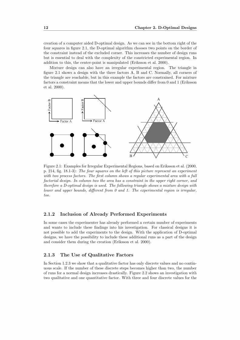
All of these areas have no restriction in the problem formulation. A restriction meansthat, e.g., one corner of the region is not accessible for experimentation. The middlecolumn of figure 2.1 shows an example of a quadratic design with a constraint in theupper right corner. This corner is not investigated and therefore a normal design isnot applicable. Reasons for this can be that the experimenter wants to prevent specialfactor combinations or that this corner cannot be investigated due to outside influences(Eriksson et al. 2000).
There are two ways to handle the irregular experimental area of figure 2.1. Theeasiest one is to shrink down the area until it has a quadratic form again, but this woulddistort the whole investigation and is not recommended. A more effective solution is the
11
12 Chapter 2. D-Optimal Designs
creation of a computer aided D-optimal design. As we can see in the bottom right of thefour squares in figure 2.1, the D-optimal algorithm chooses two points on the border ofthe constraint instead of the excluded corner. This increases the number of design runsbut is essential to deal with the complexity of the constricted experimental region. Inaddition to this, the center-point is manipulated (Eriksson et al. 2000).
Mixture design can also have an irregular experimental region. The triangle infigure 2.1 shows a design with the three factors A, B and C. Normally, all corners ofthe triangle are reachable, but in this example the factors are constrained. For mixturefactors a constraint means that the lower and upper bounds differ from 0 and 1 (Erikssonet al. 2000).
Figure 2.1: Examples for Irregular Experimental Regions, based on Eriksson et al. (2000,p. 214, fig. 18.1-3): The four squares on the left of this picture represent an experimentwith two process factors. The first column shows a regular experimental area with a fullfactorial design. In column two the area has a constraint in the upper right corner, andtherefore a D-optimal design is used. The following triangle shows a mixture design withlower and upper bounds, different from 0 and 1. The experimental region is irregular,too.
2.1.2 Inclusion of Already Performed Experiments
In some cases the experimenter has already performed a certain number of experimentsand wants to include these findings into his investigation. For classical designs it isnot possible to add the experiments to the design. With the application of D-optimaldesigns, we have the possibility to include these additional runs as a part of the designand consider them during the creation (Eriksson et al. 2000).
2.1.3 The Use of Qualitative Factors
In Section 1.2.3 we show that a qualitative factor has only discrete values and no contin-uous scale. If the number of these discrete steps becomes higher than two, the numberof runs for a normal design increases drastically. Figure 2.2 shows an investigation withtwo qualitative and one quantitative factor. With three and four discrete values for the

2.1. The Need for D-Optimal Designs 13
both qualitative factors, a full factorial design would need 4 ∗ 3 ∗ 2 = 24 design runs tosolve this problem.
The D-optimal approach reduces the number of design runs to only 12 experiments.These experiments, shown in figure 2.2 as filled circles, are chosen to guarantee a bal-anced design that is spread over the whole experimental region. ‘A balanced design hasthe same number of runs for each level of a qualitative factor’ (Eriksson et al. 2000,p. 245).
Figure 2.2: Design With Multi-Level Qualitative Factors, based on Eriksson et al. (2000,p. 214, fig. 18.4): This picture shows the experimental region for an screening investi-gation with 3 factors. Factor A and B are qualitative and have three or four discretelevels. Factor C is a normal quantitative factor with values between -1 and +1. The filledcircles represent the point chosen by an D-optimal algorithm. A full 4 ∗ 3 ∗ 2 factorialdesign would select all 24 points.
2.1.4 Reducing the Number of Experiments
The classical designs from section 1.2.3 are very inefficient if the number of factorsincreases. Table 2.1 shows examples for the minimum number of runs for a full factorial,a fractional factorial and a D-optimal design. The needed runs for a D-optimal designare always lower and do not increases as fast as the classical design with a growingnumber of factors (Umetrics 2006).
Factors Full Factorial Fractional Factorial D-Optimal
5 32 16 166 64 32 287 128 64 358 256 64 439 512 128 52
Table 2.1: Minimum Number of Design Runs for Screening Designs.

14 Chapter 2. D-Optimal Designs
2.1.5 Fitting of Special Regression Models
D-Optimal designs give the opportunity to modify the underlying model in differentways. As equation 2.1 shows, it is possible to delete selected terms if the experimenterknows that they are unimportant for the response. This allows reducing the number ofruns without having big influence on the investigation.
y = β0 + β1x1 + β2x2 + β3x3 + β12x12 +»»»»XXXXβ13x13 + β23x23 + ε (2.1)
The second possible model modification is the addition of single higher order terms.With classical designs it is only possible to change the whole model, e.g., from an inter-action to a quadratic model. In contrast to this, D-optimal designs allow the additionof independent model terms. The following equation gives an example of a linear modelwith an additional interaction term.
y = β0 + β1x1 + β2x2 + β3x3 + β23x23 + ε (2.2)
2.2 The D-Optimal Approach
A D-optimal design is a computer aided design which contains the best subset of allpossible experiments. Depending on a selected criterion and a given number of designruns, the best design is created by a selection process.
2.2.1 Candidate Set
The candidate set is a matrix that contains all theoretically and practically possibleexperiments, where ‘each row represents an experiment and each columns a variable’(de Aguiar et al. 1995, p. 201). This so-called matrix of candidate points has N rowsand is represented by ξN .
For a simple investigation with two factors, x1 and x2, the candidate set has twocolumns and four rows. We get four rows because we only consider the 2k experimentswhich have a minimum or maximum value for the factors. The selection of other ex-periments can be useful in special cases but is not considered in this basic example.Equation 2.3 shows the candidate set in the extended notation.
ξ4 =
−1 −1−1 11 −11 1
(2.3)
2.2.2 Design Matrix
The design matrix X is a n × p matrix that depends on a model with p coefficients.The number of rows n can be chosen by the experimenter and represents the number ofexperiments in the design. With a given model and a candidate matrix, the constructionof the design matrix is easy. Each column contains a combination of the factors fromthe candidate set, depending on the terms in the model. The matrix can also be calledmodel matrix, but in most cases the model matrix means a N×p matrix which containsthe model-dependent rows for all candidates (de Aguiar et al. 1995).

2.3. Criteria for the Best D-Optimal Design 15
We use the earlier candidate set ξ4 and the model from equation 2.4 for a simpleexample with n = 4 design runs.
y = β0 + β1x1 + β2x2 + β12x1x2 + ε (2.4)
As a result, we have a model matrix with four rows and four columns, where all candi-dates from ξ4 are used in the design. Normally, the candidate set contains much moreexperiments and the model matrix is only a small subset.
X =
1 −1 −1 11 −1 1 −11 1 −1 −11 1 1 1
(2.5)
The first column of X represents the constant term β0, so it only contains ones. Columntwo and three are the model terms for the investigated factors, x1 and x2, taken fromthe candidate set ξ4. The last column of X represents an interaction between the bothfactors. Hence, we have to multiply the two columns from the candidate set.
With a bigger candidate set, the number of possible subsets of ξN increases and theselection of the design matrix has to be done depending on a special criterion. ‘Thebest combination of these points is called optimal and the corresponding design matrixis called optimal design matrix’ X* (de Aguiar et al. 1995, p. 202). We deal with thedifferent criteria in section 2.3.
2.2.3 Information and Dispersion Matrix
To use the later described criteria for the selection of the best design, we need to definetwo other types of matrices. The first one is the so-called information matrix (X ′X).This matrix is the multiplication of the transpose of the design matrix X ′ and X itself.The dispersion matrix (X ′X)−1 is the inverse matrix of this calculation (de Aguiaret al. 1995). The background of these equations can be found in the least-squaresestimate β for an assumed model. A model with the matrix notation
y = Xβ + ε (2.6)
has the best set of coefficients according to least squares given by
β = (X ′X)−1X ′y. (2.7)
Further information on the least square estimator can be found in Box et al. (1978) orWu & Hamada (2000).
2.3 Criteria for the Best D-Optimal Design
In the following section, we discuss the different criteria for a D-optimal design. All ofthem belong to the group of information-based criteria because they try to maximizethe information matrix (X ′X).

16 Chapter 2. D-Optimal Designs
D-Optimality (Determinant)
The D-Optimality is the most common criterion ‘which seeks to maximize |X ′X|, thedeterminant of the information matrix (X ′X) of the design’ (NIST/SEMATECH 2007,ch. 5.5.2). This means that the optimal design matrix X* contains the n experimentswhich maximizes the determinant of (X ′X). Or in other words, the n runs ‘span thelargest volume possible in the experimental region’ (Eriksson et al. 2000, p. 216). Equa-tion 2.8 shows the selection of X* out of all possible design matrices chosen from ξN .This connection between the design matrix and the determinant also explains the useof the “D” in the term D-optimal designs.
∣∣X*′X*∣∣ = max
ξnΞN
(|X ′X|) (2.8)
Maximizing the determinant of the information matrix (X ′X) is equivalent to minimiz-ing the determinant of the dispersion matrix (X ′X)−1. This correlation is very usefulto keep the later calculations as short as possible.(de Aguiar et al. 1995).
|X ′X| = 1|(X ′X)−1| (2.9)
A-Optimality (Trace)
Another criterion for an optimal design is called the A-criterion. The design matrix isconsidered as A-optimal when the trace of the dispersion matrix (X ′X)−1 is minimum.In this case, the trace of the square matrix is the sum of the elements on the main diag-onal. Minimizing the trace of the matrix is similar to minimizing the average varianceof the estimated coefficients.
trace(X*′X*)−1 = minξnΞN
(trace(X ′X)−1
)(2.10)
trace(X ′X)−1 =p∑
i=1
cii (2.11)
A-optimal designs are rarely used because it is more computationally difficult to updatethem during the selection process.
V-optimality (Average Prediction Variance)
As de Aguiar et al. (1995, p. 203) describe, ‘the variance function or leverage is ameasurement of the uncertainty in the predicted response’. This variance of predicationfor a single candidate χi can be calculated with the equation
d(χi) = χ′i ∗ (X ′X)−1 ∗ χi, (2.12)
where χi equals a vector that describes a single experiment and χ′i represents the trans-pose of this vector. With the selection of a V-optimal design, the choose candidateshave the lowest average variance of prediction, as shown in equation 2.13.
1n
n∑
i=1
χ′i ∗ (X*′X*)−1 ∗ χi = minξnΞN
(1n
n∑
i=1
χ′i ∗ (X ′X)−1 ∗ χi
)(2.13)

2.4. A Basic Example 17
G-Optimality (Maximum Prediction Variance)
The last criterion is called G-optimal and deals also with the variance of prediction ofthe candidate points. The selected optimal design matrix is chosen to minimize thehighest variance of prediction in the design.
max(χ′i ∗ (X*′X*)−1 ∗ χi
)= min
ξnΞN
(max
(χ′i ∗ (X ′X)−1 ∗ χi
))(2.14)
G-Efficiency
In most cases, the G-criterion is not used to find the best design during the selectionprocess but is applied to choose between several similar designs which were created withanother criterion, like D-optimality. For this comparison the so-called G-efficiency isused. It is defined by
Geff = 100% ∗(
p
n ∗ dmax(χ)
), (2.15)
where p is the number of model terms or coefficients, n is the number of design runs anddmax(χ) is the largest variance of prediction in the model matrix X. The G-efficiencycan be seen as a comparison of a D-optimal design and a fractional factorial design.Consequently, the efficiency is given in a percentage scale.
Condition Number
The condition number (CN) is an evaluation criteria like the G-efficiency and is used torate an already created D-optimal design. It evaluates the sphericity and the symmetryof the D-optimal design by calculating ‘the ratio between the largest and smallest sin-gular values of’ X (Eriksson et al. 2000, p. 220). A design with a condition number of 1would be orthogonal, while an increasing condition number indicates a less orthogonaldesign.
2.4 A Basic Example
This example is taken from Eriksson et al. (2000) and uses an investigation with twofactors, x1 and x2, to demonstrate the D-optimal approach in a geometrical way. Thetwo factors are investigated in three levels, -1, 0 and 1. The corresponding candidateset is listed in table 2.2.
Nr. 1 2 3 4 5 6 7 8 9
x1 -1 -1 -1 0 0 0 1 1 1x2 -1 0 1 -1 0 1 -1 0 1
Table 2.2: Candidate Set for Two Factors with Three Levels.
If we would display the candidate set with the matrix notation, the matrix ξ9 wouldcontain two columns, one for each factor, and N = 9 experiments. Figure 2.3 shows thenine candidates from ξ9 as a plot over the experimental area.
Considering a design with only three design runs, we have 9!/(3! ∗ 6!) = 84 possiblesubsets out of this candidate set. In this example, we evaluate four possible design

18 Chapter 2. D-Optimal Designs
Figure 2.3: Distribution of the Candidate Set, based on Eriksson et al. (2000, p. 218,fig. 18.22): This picture shows the distribution of the candidates over the experimentalregion. The investigation considers two factors with three levels and therefore ninecandidate points.
matrices and compare them depending on the D-criteria. Equation 2.16 shows the fourselected subset in the matrix notation and figure 2.4 displays the experimental regionwith the corresponding candidates.
ξ3A =
−1 −10 01 1
, ξ3B =
0 −1−1 00 1
, ξ3C =
−1 −11 00 1
, ξ3D =
−1 −11 −1−1 1
(2.16)
Figure 2.4: Distribution of the Design Matrix, based on Eriksson et al. (2000, p. 218,fig. 18.23-27): For four different design matrices, the distribution of the selected candi-dates is shown over the experimental region. The designs are taken from the candidateset ξ9 from figure 2.3.
To compute the optimality of these designs, we need to select a model first. In orderto keep the example as simple as possible, we choose the following linear model:
y = β0 + β1x1 + β2x2 + ε. (2.17)
Comparing the designs depending on the D-criterion is only possible if we calculate thedeterminants of the information matrix (X ′X) for each of the four designs. In thisexample, we only show the calculation for the subset ξ3B , but the principle will be thesame for all. First, we have to create the model depending design matrix X and itstranspose X ′. With the linear model, we have a simple design matrix that containsthe constant β0 in the first column and the two factors in the following columns. The
2.5. Fitting the Model 19
calculation of the information matrix is simple the multiplication of these both matrices.
(X ′BXB) =
1 1 10 −1 0−1 0 1
∗
1 0 −11 −1 01 0 1
=
3 −1 0−1 1 00 0 2
(2.18)
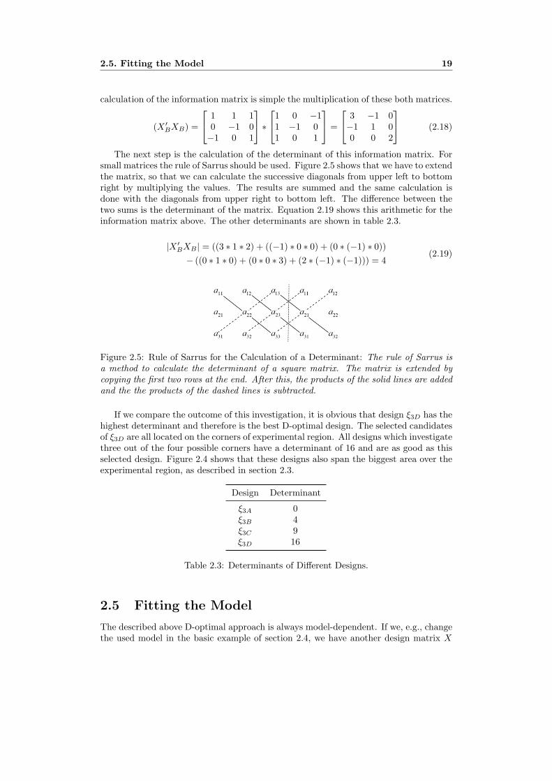
The next step is the calculation of the determinant of this information matrix. Forsmall matrices the rule of Sarrus should be used. Figure 2.5 shows that we have to extendthe matrix, so that we can calculate the successive diagonals from upper left to bottomright by multiplying the values. The results are summed and the same calculation isdone with the diagonals from upper right to bottom left. The difference between thetwo sums is the determinant of the matrix. Equation 2.19 shows this arithmetic for theinformation matrix above. The other determinants are shown in table 2.3.
|X ′BXB | = ((3 ∗ 1 ∗ 2) + ((−1) ∗ 0 ∗ 0) + (0 ∗ (−1) ∗ 0))− ((0 ∗ 1 ∗ 0) + (0 ∗ 0 ∗ 3) + (2 ∗ (−1) ∗ (−1))) = 4
(2.19)
Figure 2.5: Rule of Sarrus for the Calculation of a Determinant: The rule of Sarrus isa method to calculate the determinant of a square matrix. The matrix is extended bycopying the first two rows at the end. After this, the products of the solid lines are addedand the the products of the dashed lines is subtracted.
If we compare the outcome of this investigation, it is obvious that design ξ3D has thehighest determinant and therefore is the best D-optimal design. The selected candidatesof ξ3D are all located on the corners of experimental region. All designs which investigatethree out of the four possible corners have a determinant of 16 and are as good as thisselected design. Figure 2.4 shows that these designs also span the biggest area over theexperimental region, as described in section 2.3.
Design Determinant
ξ3A 0ξ3B 4ξ3C 9ξ3D 16
Table 2.3: Determinants of Different Designs.
2.5 Fitting the Model
The described above D-optimal approach is always model-dependent. If we, e.g., changethe used model in the basic example of section 2.4, we have another design matrix X

20 Chapter 2. D-Optimal Designs
and consequently another information matrix (X ′X). Hence, the selection of the modelis an important step of the problem formulation. In section 1.2.5, we explain the basicmodel concept with an example of a linear model. In the following paragraphs, thismodel is used, and in some case also interaction or quadratic terms are mentioned. Tohandle more complex investigations, we examine these models in more detail.
Linear Models
Linear models are used for screening designs or robustness tests. Inside the model eachfactor only appears as a linear term. In this case, a linear term means a combinationof a coefficient βi and a factor xi. A linear model with three factors has the followingequation:
y = β0 + β1x1 + β2x2 + β3x3 + ε. (2.20)
Interaction Models
Interaction models are more complex than linear ones but are used for the same exper-imental objectives as their linear counterpart. The interaction model contains the sameterms like the linear model but has additional interaction terms. An interaction term isthe combination of two factors xi and xj with a conjoint coefficient βij . Equation 2.21gives an example of an interaction model with three factors.
y = β0 + β1x1 + β2x2 + β3x3 + β12x1x2 + β13x1x3 + β23x2x3 + ε (2.21)
Quadratic Models
The third commonly used model is the quadratic model. It extends the interactionmodel with additional quadratic terms for each factor. A quadratic term is the squareof a factor xi with its coefficient βii. Quadratic models are the most complex of thethree basic model types and are used for optimization processes. In the same way asthe former models, a quadratic model with three factors has the following equation:
y = β0 + β1x1 + β2x2 + β3x3 + β11x21 + β22x
22 + β33x
23
+β12x1x2 + β13x1x3 + β23x2x3 + ε.(2.22)
2.6 Scaling
Scaling means that the raw data, which has different upper and lower bounds for eachfactor, is reduced to a set of data where all factors have the same range. We use a kindof scaling in section 1.3.2 when we explain the general and extended notation to displaythe candidate set. Scaling can be done in three different ways. For D-optimal designsthe orthogonal scaling is the most common, but the other ones are applicable, too.
Orthogonal Scaling
When an orthogonal scaling is performed, the factors are scaled and centered dependingon the high and low values from the factor definition and the midrange of the values.An original factor xi is scaled as follows:
zi =xi − M
R, (2.23)
2.7. Number of Design Runs 21
where M is the midrange of all values in the candidate set and R represents the rangebetween the high and low value from the factor definition.
M =max x + min x
2, R =
max xdef −min xdef
2(2.24)
Midrange Scaling
A midrange scaling only centers the values depending on the midrange of the highestand lowest factor value in the candidate set. The values are not scaled. Equation 2.25gives the arithmetic for this calculation.
zi = xi − M (2.25)
Unit Variance Scaling
The last scaling is called unit variance scaling and also uses the midrange of the highestand lowest factor value to center the data. In addition to this, a scaling depending onthe standard deviation σ of the values is performed. The following equation shows thecalculation for an unscaled factor xi.
zi =xi − M
σ(2.26)
2.7 Number of Design Runs
In order to fit a optimality criterion from section 2.3, we have to define the numberof experiments we want to have in the design. The selection of this factor n is veryimportant because changing the number of the design runs alters the model matrix andanother optimal design is chosen. There are no rules to define this number, but theminimum is model-dependent. A model with p coefficients can only be investigatedwith a D-optimal design which has at least p runs. In most cases, it is useful to createdifferent designs that differ in the number of runs and compare the efficiency of thedesigns. A design with a few more or less design runs than the desired one can have ahigher determinant and hence is the best design to perform.
2.8 Bayesian Modification
D-optimal designs use different criteria to choose the best design from a pool of allpossible factor combinations. For all these criteria, the selection process is stronglymodel-dependent and therefore the experimenter should pay attention to the choice ofthe model. Changing one or more coefficients creates a different model matrix whichleads to another optimal design.
2.8.1 The Addition of Potential Terms
This dependence on the assumed model can be a problem if the model is not chosencarefully. A Bayesian modification reduces this influence of the model by adding addi-tional potential terms. Considering a model with p primary terms, we add q potentialterms and the model matrix X has the following form:
X = (Xpri|Xpot). (2.27)

22 Chapter 2. D-Optimal Designs
The additional terms are normally not included in the model and have a higher degreethan the primary terms. The selection of the potential terms is problem-dependent andis explained in detail in chapter 4 (DuMouchel & Jones 1994).
2.8.2 Scaling the Factors
In order to profit from the Bayesian modification, the primary and potential terms haveto be scaled in different ways. Each non constant primary term has a range of 2 andvaries from -1 to 1. Normally, these terms are scaled and centered with the orthogonalscaling.
max(Xpri) = 1, min(Xpri) = −1 (2.28)
For the Bayesian modification, DuMouchel & Jones (1994, p. 39) defined that the po-tential terms have the following condition:
max(Xpot)−min(Xpot) = 1, (2.29)
where the maximum and minimum values ‘are taken over the set of candidate points forthe design’. The scaling of the potential terms is ‘achieved by performing a regression ofthe potential terms on the primary terms, using the candidate points [. . . ] to computeα and Z’ (DuMouchel & Jones 1994, p. 40).
α = (X ′priXpri)−1 ∗X ′
priXpot (2.30)
R = Xpot −Xpri ∗ α (2.31)
Z =R
max(R)−min(R)(2.32)
In this case, α is the least square coefficient of Xpot on Xpri and R represents the residualof this regression. The used minimum and maximum values are taken column-wise overthe whole candidate set. The outcoming matrix Z is the scaled and centered version ofthe potential terms and is used in the model matrix instead of Xpot.
X = (Xpri|Z) (2.33)
To use the Bayesian modified model matrix with normal D-optimal criteria, we haveto update the dispersion matrix (X ′X)−1 by adding a further matrix. This so-calledQ-matrix is a (p+q)× (p+q) diagonal matrix with zeros in the first p diagonal elementsand ones in the last q diagonal elements. Depending on a chosen τ -value, we modify thedispersion matrix as follows: (
X ′X +Q
τ2
)−1
. (2.34)
DuMouchel & Jones (1994, p. 40) defined that ‘[t]he value τ = 1 is a suitable defaultchoice, implying that the effect of any potential term is not expected to be much largerthan the residual standard error’.
2.8. Bayesian Modification 23
2.8.3 Bayesian Example
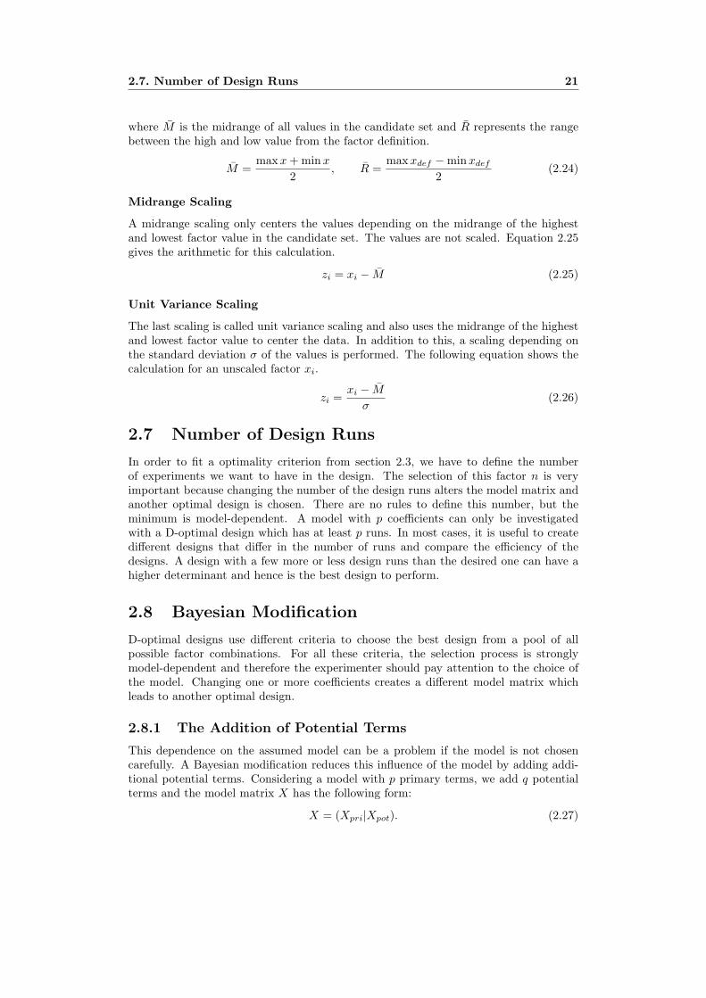
Using the basic example from section 2.4 and increasing the number of design runsto n = 5, a normal selection process with D-optimality as estimation criterion createsan optimal design X*
norm that chooses all four corners of the experimental region. Inaddition to this, the fifth point is a replicate of one of the already selected corners.The left area in figure 2.6 shows a possible combination of the five selected points, andequation 2.35 gives the matrix notation. The calculated determinant for this optimaland model-dependent design is 512.
X*norm =
1 −1 −1 11 −1 1 −11 1 −1 −11 1 1 11 −1 1 −1
(2.35)
A Bayesian modification changes the selection process by modifying the model matrixwith additional potential terms. The selected experiments are displayed in figure 2.6 onthe right side. In our example, we use the simple interaction model from equation 2.17and add the pure quadratic terms β11x
21 and β22x
22. With this modification, the primary
and potential terms of the optimal design matrix X*bay have the following form:
X*bay,prim =
1 −1 −1 11 −1 1 −11 1 −1 −11 1 1 11 0 0 0
, X*bay,pot =
1 11 11 11 10 0
(2.36)
The primary term matrix contains four model-dependent columns, where the first onerepresents the constant, column two and three are the normal factors x1 and x2, andthe last column contains the interaction term x1 ∗ x2. The two columns of the potentialterm matrix are simply the squares of the factors x1 and x2.
Figure 2.6: Distribution of Normal and Bayesian Design Matrix, based on DuMouchel &Jones (1994, p. 42, fig. 1): This picture shows the distribution of the selected candidatesby a normal D-optimal selection process on the left and the Bayesian modification onthe right. The candidates are shown over the experimental region and taken from thecandidate set ξ9 from section 2.4.
After the Bayesian scaling of the potential terms, we combine the primary termmatrix with the modified potential matrix Z. Equation 2.37 shows the new design

24 Chapter 2. D-Optimal Designs
matrix X*bay with the scaled potential terms in the last two columns. The lower values
of the q additional terms shows that the terms in Z are less important than the p primaryterms in the original design matrix.
X*bay =
1 −1 −1 1 0.2 0.21 −1 1 −1 0.2 0.21 1 −1 −1 0.2 0.21 1 1 1 0.2 0.21 0 0 0 −0.8 −0.8
(2.37)
To complete this example, we have to add the Q-Matrix to the dispersion matrix(X ′X)−1 before we can select the optimal design matrix X*
bay with the highest de-terminant. For our investigation with p = 4 primary and q = 2 potential terms, Q is a6× 6 diagonal matrix with the following values:
Q =
0 0 0 0 0 00 0 0 0 0 00 0 0 0 0 00 0 0 0 0 00 0 0 0 1 00 0 0 0 0 1
. (2.38)
A comparison of the two designs with the D-optimal criterion shows that the determi-nant, taken over the primary terms, of the matrix X*
norm is higher than the determinantof X*
bay. However, an observation of figure 2.6 indicates that a Bayesian modified versionof the D-optimal approach selects a better design, without duplicates. In addition tothis, the selection is minor model-dependent.
∣∣∣X*′normX*
norm
∣∣∣ = 516,∣∣∣X*′
bay,primX*bay,prim
∣∣∣ = 320 (2.39)

Chapter 3
D-Optimal Designs as aComputer Algorithm
3.1 Exchange Algorithms
Chapter 2 describes the basic principles and criteria for the construction of D-optimaldesigns but does not explain the selection process itself. Based on the complexity ofthe D-optimal designs and the huge number of possible combinations of experiments,computer algorithms are used for the selection process. The present thesis only dealswith the so-called exchange algorithms. Figure 3.1 summarizes the basic steps whichhave to be performed before such an exchange algorithm is applicable.
Figure 3.1: Flow Chart of the D-Optimal Process.
An exchange algorithm selects the optimal design matrix X* by exchanging one ormore points from a generated start design and repeats this exchanges until the bestmatrix seems to be found. The algorithms can be differentiated in two groups where arank-1 algorithm adds and deletes the points sequentially, and a rank-2 algorithm realizesthe exchange by a simultaneous adding and deleting process (Meyer & Nachtsheim 1995).We now explain and evaluate six different algorithms which are universally applicable
25

26 Chapter 3. D-Optimal Designs as a Computer Algorithm
but differ in the used computing time and the quality or efficiency of the generateddesigns.
3.1.1 General Exchange Procedure
In order to begin the selection process, we have to create a start design with n experi-ments in the design matrix Xn. The aim of an exchange algorithm is to remove or addpoints to this design matrix and determine the effect of the modification. With referenceto section 2.2, we call the information matrix (X ′
nXn) and use the following equationfor the variance of prediction of a single candidate χx:
d(χx) = χ′x ∗ (X ′nXn)−1 ∗ χx. (3.1)
The addition of a new experiment χj to the design matrix Xn, creates a new matrixXn+1, and as de Aguiar et al. (1995) showed, the relation between these two matricescan be expressed by the use of the information matrices. Equation 3.2 shows thisinterconnection with the use of the added single candidate χj and its transpose.
(X ′n+1Xn+1) = (X ′
nXn) + (χj ∗ χ′j) (3.2)
Furthermore, the influence of the exchange can be used to update the determinant ofthe new matrix without calculating it in the ordinary way. In this case, the determinantincreases proportional to the variance of prediction d(χj) of the added point χj .
∣∣X ′n+1Xn+1
∣∣ = |X ′nXn| ∗ (1 + d(χj)) (3.3)
Removing an experiment χi from the design matrix relies on the same fundamentalsand is given with the following equations:
(X ′n−1Xn−1) = (X ′
nXn)− (χi ∗ χ′i), (3.4)∣∣X ′
n−1Xn−1
∣∣ = |X ′nXn| ∗ (1− d(χi)) . (3.5)
The selection of the added and removed points among the candidate set is different ineach algorithm and is discussed in the following sections (de Aguiar et al. 1995).
3.1.2 DETMAX Algorithm
The DETMAX algorithm was published by Mitchell (1974) and is a typical rank-1algorithm. With a random start design of n runs, the algorithm tries to improve thedeterminant of the information matrix by either adding or deleting a point. The addedexperiment χj is the one with the highest variance of prediction d(χj). As equation 3.3shows, this experiment leads to the maximum possible increase of the determinant. Thedeleted point χi is the one with the lowest variance of prediction because an exchangeof this point decreases the determinant the least. If a point is added or deleted first, ischosen randomly. The result of such an exchange process is a determinant that is higheror equal than the previous one.
So far this algorithm would be the Wynn-Mitchell algorithm from 1972, but Mitchell(1974) modified this approach to gain more flexibility and allowed excursions in thedesign. In this case, an excursion means that a n + 1-point design must not be reducedimmediately to a n-point design but can become a design with n + 2 points. Therefore,the replacement of more than one point of the original design can be possible during one

3.1. Exchange Algorithms 27
iteration. The limit of excursions is defined by Mitchell (1974) to be k = 6. Consideringa design with the currently best n points, the algorithm adds or deletes up to k pointsuntil the excursion limit is reached. The size of the created designs varies from n − kto n + k. If no improvement in the determinant is found during this excursion, all thecreated design are saved in a list F that contains failure designs. This set F is usedfor the next excursion where we consider two different rules defined by Mitchell (1974,p. 204):
Letting D be the current design at any point during the course of an excur-sion, the rules for continuing are as follows:
(i) If the number of points in D exceed n, subtract a point if D is not inF and add a point otherwise.
(ii) If the number of points in D is less than n, add a point if D is not inF and subtract a point otherwise.
The following listing 3.1 shows the use of these excursion rules and visualizes the flowof the algorithm with a simple and abstract programming notation.
create random design with desired number of points;while excursion limit is not reached do
if number of candidates equals number of desired runs thenrandomize between adding or deleting a point;
else if number of candidates is bigger than number of desired runs thenif new designs is not inside set of failure design then
delete candidate with lowest variance of prediction;else
add candidate with highest variance of prediction;
else if number of candidates is smaller than number of desired runs thenif new designs is not inside set of failure design then
add candidate with highest variance of prediction;else
delete candidate with lowest variance of prediction;
if no improvement of the determinant is found thensave design to list of failure designs;
elseclear list of failure designs;
Algorithm 3.1: DETMAX algorithm by Mitchell (1974).

28 Chapter 3. D-Optimal Designs as a Computer Algorithm
With an empty set of failure designs F , the algorithm simply adds and subtractspoints, as described in the first paragraph of this section. Considering the failure designsof previous iterations, the algorithm always ‘proceeds in the direction of a n-point design,unless it comes to a design in F , which has already lead to failure. Then it reversesdirection [. . . ]’ (Mitchell 1974, p. 204). If an excursion improves the design, the failuredesigns in F are deleted and a new start is performed (de Aguiar et al. 1995, Mitchell1974).
3.1.3 Fedorov Algorithm
Fedorov’s (1972) algorithm is a simultaneous exchange method which always keeps thesize n of the desired design without any excursions. After the generation of a randomstart design, the algorithm selects a point χi from the design that should be removedby a point χj from the candidate set. The procedure of adding and removing a point isdone in one step and can be denoted as a real exchange. The effect of such an exchangecan be shown by the use of the information matrix. With reference to equation 3.2 and3.4, an exchange is a simultaneous addition and subtraction of a point.
(X ′newXnew) = (X ′
oldXold)− (χi ∗ χ′i) + (χj ∗ χ′j) (3.6)
In contrast to the general exchange from section 3.1.1, Fedorov (1972) considered theinteraction between the variance functions of the two candidates for the calculation ofthe new determinant. Instead of adding and deleting the variance of prediction of thetwo points according to equation 3.3 and 3.5, he defined a so-called “delta”-functionwhich changes the determinant of the the matrix in the following way:
|X ′newXnew| = |X ′
oldXold| ∗ (1 + ∆(χi, χj)) . (3.7)
The calculation of the ∆-value for a couple of χi and χj uses the variance of predictionof both points and a combined variance function called d(χi, χj).
∆(χi, χj) = d(χj)−[d(χi) d(χj)− (d(χi, χj))
2]− d(χi) (3.8)
d(χi, χj) = χ′i ∗ (X ′nXn)−1 ∗ χj = χ′j ∗ (X ′
nXn)−1 ∗ χi (3.9)
The basic idea of the Fedorov algorithm is to calculate the ∆-value for all possiblecouples (χi,χj) and select the one with the highest value. The point χi is taken from thecurrently selected design, and χj can either be taken from the remaining points or fromthe whole candidate set. Considering only the remaining points is called an exhaustingsearch which avoids duplicated points in the design. With a non-exhausting search, theselection of an experiment which has to be performed twice is possible. As equation 3.7shows, the points with the highest ∆-value increase the determinant most. If more thanone couple with the same ∆-value is found, the algorithm chooses randomly among them.While couples with a positive ∆-value are found, the algorithm exchanges the points andupdates the information and dispersion matrix. Sometimes the algorithm finds couplesthat increase the determinant so little that no significant difference is achieved. Toavoid the algorithm dealing with the exchange of these couples, Fedorov (1972) defineda threshold value εfed and breaks the algorithm if the maximum ∆-value is smaller thanεfed. 10−6 is a common value for εfed (de Aguiar et al. 1995, Fedorov 1972). The generaloutline of the algorithm is given in listing 3.2.

3.1. Exchange Algorithms 29
create random design with desired number of points;while couples with positive delta are found do
for design point χ1 to design point χn docalculate variance of prediction d(χi) for this design point;for support point χ1 to support point χN do
calculate variance of prediction d(χj) for this support point;calculate variance function d(χi, χj) for this couple;calculate delta function ∆(χi, χj) for this couple;check if maximum delta and save couple;
if maximum delta is positive thenif more then one couple with same maximum delta then
select couple randomly;exchange selected point χi with χj ;update information and dispersion matrix;reset maximum delta;
Algorithm 3.2: Fedorov Algorithm (1972).
3.1.4 Modified Fedorov Algorithm
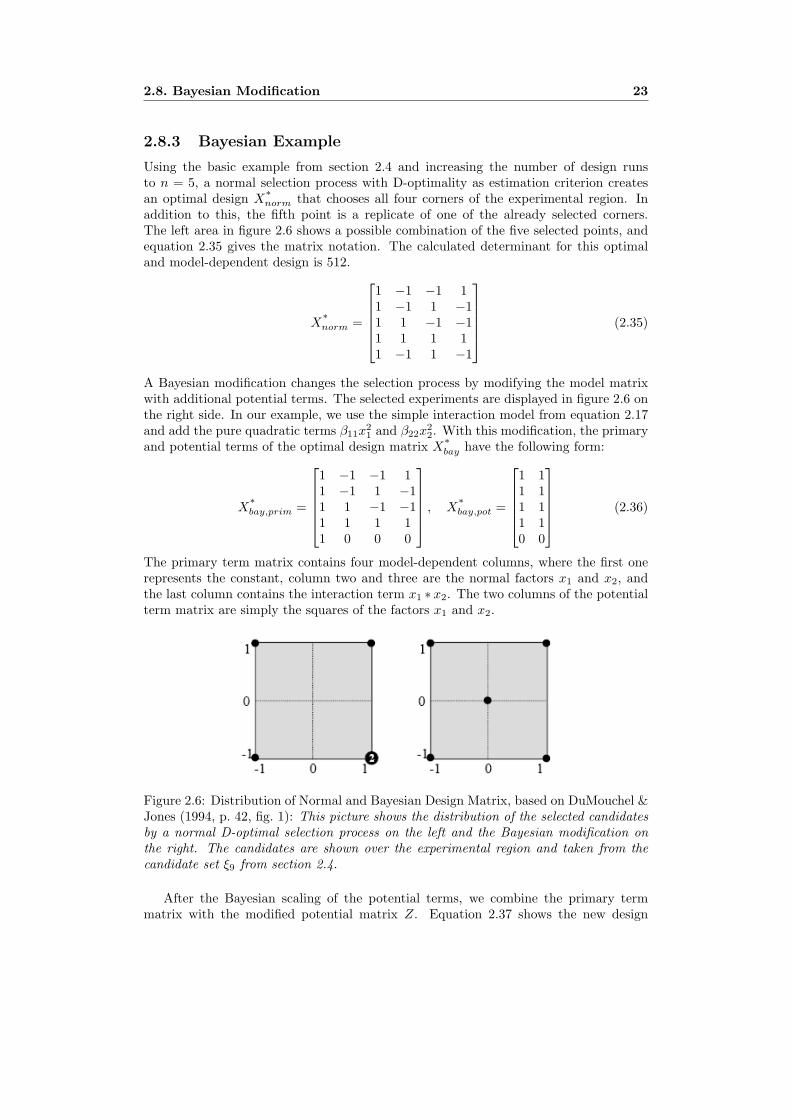
Cook & Nachtsheim (1980) made a comparison of different algorithms for constructingexact D-optimal designs and invented an own algorithm depending on the basic Fedorovalgorithm from 1972. The normal algorithm by Fedorov calculates the ∆-values for allpossible exchange couples during one iteration but only uses one of the values to performan exchange. This calculation is expensive to use. With the modified version by Cook& Nachtsheim (1980, p. 317), each iteration of the normal algorithm ‘is broken downinto [n] stages, one for each support point in the design at the start of the iteration.’With a randomly ordered design matrix, the algorithm starts with the first supportpoint χi and calculates the ∆-values for all possible couples with this fixed supportpoint. After finding the best exchange for this point, the design is updated and the nextsupport point is suggested for an exchange. In other words, one iteration of the normalFedorov algorithm is modified to exchange up to n design points if the determinantwould increase (Cook & Nachtsheim 1980, Atkinson & Donev 1989). This behavior isvisualized in listing 3.3.
The difference between the two approaches can be made clear with a simple example.Considering a desired design with n = 5 runs and a candidate set with N = 20 experi-ments, n ∗N = 100 possible couples can be suggested for an exchange. Each iterationof the Fedorov algorithm calculates these 100 ∆-values for all possible couples and usesonly one of them for an exchange. By contrast, the modified version of the algorithmstarts with the first design point and only calculates the 20 ∆-values for the possiblecouples including this point. After this, an exchange is performed and the dispersionmatrix has to be updated. The algorithm goes on with the next design point and cal-culates again 20 ∆-values. Overall, both algorithm calculate the 100 values during oneiteration, but the modified version exchanges up to 5 points during this procedure.
A study by Cook & Nachtsheim (1980) and the data presented in the followingchapter 3.3 show that the modified approach can be twice as fast as the normal Fedorov
30 Chapter 3. D-Optimal Designs as a Computer Algorithm
create random design with desired number of points;while couples with positive delta are found do
for design point χ1 to design point χn docalculate variance of prediction d(χi) for this design point;for support point χ1 to support point χN do
calculate variance of prediction d(χj) for this support point;calculate variance function d(χi, χj) for this couple;calculate delta function ∆(χi, χj) for this couple;select couple with maximum delta;if maximum delta is positive then
if more then one couple with same maximum delta thenselect couple randomly;
exchange selected point χi with χj ;update information and dispersion matrix;reset maximum delta;
Algorithm 3.3: Modified Fedorov Algorithm by Cook & Nachtsheim (1980).
algorithm and creates design with a comparable efficiency. The additional time neededto update the dispersion matrix after each exchange is adjusted by the profit of themultiple exchanges.
3.1.5 k-Exchange Algorithm
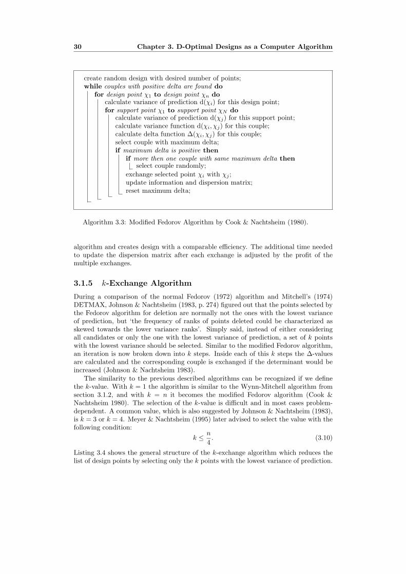
During a comparison of the normal Fedorov (1972) algorithm and Mitchell’s (1974)DETMAX, Johnson & Nachtsheim (1983, p. 274) figured out that the points selected bythe Fedorov algorithm for deletion are normally not the ones with the lowest varianceof prediction, but ‘the frequency of ranks of points deleted could be characterized asskewed towards the lower variance ranks’. Simply said, instead of either consideringall candidates or only the one with the lowest variance of prediction, a set of k pointswith the lowest variance should be selected. Similar to the modified Fedorov algorithm,an iteration is now broken down into k steps. Inside each of this k steps the ∆-valuesare calculated and the corresponding couple is exchanged if the determinant would beincreased (Johnson & Nachtsheim 1983).
The similarity to the previous described algorithms can be recognized if we definethe k-value. With k = 1 the algorithm is similar to the Wynn-Mitchell algorithm fromsection 3.1.2, and with k = n it becomes the modified Fedorov algorithm (Cook &Nachtsheim 1980). The selection of the k-value is difficult and in most cases problem-dependent. A common value, which is also suggested by Johnson & Nachtsheim (1983),is k = 3 or k = 4. Meyer & Nachtsheim (1995) later advised to select the value with thefollowing condition:
k ≤ n
4. (3.10)
Listing 3.4 shows the general structure of the k-exchange algorithm which reduces thelist of design points by selecting only the k points with the lowest variance of prediction.

3.1. Exchange Algorithms 31
create random design with desired number of points;while couples with positive delta are found do
calculate variance of prediction d(χi) for all design points;select k design points with lowest variance of prediction;for design point χ1 to design point χk do
calculate variance of prediction d(χi) for this design point;for support point χ1 to support point χN do
calculate variance of prediction d(χj) for this support point;calculate variance function d(χi, χj) for this couple;calculate delta function ∆(χi, χj) for this couple;select couple with maximum delta;if maximum delta is positive then
if more then one couple with same maximum delta thenselect couple randomly;
exchange selected point χi with χj ;update information and dispersion matrix;reset maximum delta;
Algorithm 3.4: k-Exchange Algorithm by Johnson & Nachtsheim (1983).
Continuing the example with n = 5 and N = 20, the k-exchange speeds up theselection process by reducing the complete number of calculated ∆-values. Similar tothe modified Fedorov procedure, each iteration of the basic Fedorov algorithm is brokendown into ∆-calculations for each design point. But depending on the defined k-value,the algorithm only considers some of the design points. With k = 3 the k-exchangealgorithm calculates three times the 20 ∆-values and performs up to three exchanges.This approach has a higher computational efficiency compared to the modified Fedorovprocedure. Especially for huge data set with a high value of n, the definition of thek-value has an impact. The quality of the design is not always as good as the onefrom the normal Fedorov algorithm, but with respect to the needed computing time,the algorithm gives good results. A detailed analysis of the efficiency and quality of thedesigns follows in section 3.3.
3.1.6 kl-Exchange Algorithm
The kl-exchange is also a modification of the basic Fedorov algorithm from 1972 andtherefore a typical rank-2 algorithm. Developed by Atkinson & Donev (1989), thisalgorithm reduces the list of support and exchange points before calculating the ∆-values for all possible couples. The use of the k points with the lowest variance ofprediction is similar to the k-exchange procedure. In addition to this, we only considerthe l candidates with the highest variance of prediction among the support points. Bydefining k = n and l = N , this algorithm is the normal Fedorov procedure. A normalinitialization of the algorithm with k < n and l < N reduces the amount of calculated ∆-values and speed up the algorithm. Like the normal Fedorov algorithm, the kl-exchangeselects the points with the highest ∆-value and performs a single exchange. Even ifthe name of the kl-exchange sound like a modification of the k-exchange by Cook &

32 Chapter 3. D-Optimal Designs as a Computer Algorithm
Nachtsheim (1980), we have to observe that the kl-procedure relies on the basic Fedorovalgorithm and does not perform multiple exchanges during one iteration. Only theconcept of picking the k point with the lowest variance of prediction is similar to thek-exchange algorithm.
Atkinson & Donev (1989) defined two modifications of this algorithm. The first oneis similar to the basic idea of the modified Fedorov algorithm by Cook & Nachtsheim(1980) and performs more than one exchange during each iteration. With the selectionof l = 1, this changed kl-exchange becomes either the modified Fedorov algorithm withk = n or the k-exchange with k < n. The second modification changes the selectioncriteria for the k and l points. Instead of a variance dependent choice, the algorithmselects randomly among the design and support points (Atkinson & Donev 1989). Inlisting 3.5 the basic version is shown without any modification.
create random design with desired number of points;while couples with positive delta are found do
calculate variance of prediction d(χi) for all design points;select k design points with lowest variance of prediction;calculate variance of prediction d(χj) for all support points;select l support points with highest variance of prediction;for design point χ1 to design point χk do
calculate variance of prediction d(χi) for this design point;for support point χ1 to support point χl do
calculate variance of prediction d(χj) for this support point;calculate variance function d(χi, χj) for this couple;calculate delta function ∆(χi, χj) for this couple;check if maximum delta and save couple;
if maximum delta is positive thenif more then one couple with same maximum delta then
select couple randomly;exchange selected point χi with χj ;update information and dispersion matrix;reset maximum delta;
Algorithm 3.5: kl-Exchange Algorithm by Atkinson & Donev (1989).
Compared with the normal Fedorov algorithm, the kl-exchange reduces the amountof calculated ∆-values between each iteration. Our example with n = 5, N = 20 andk = l = 3 leads to the calculation of only k ∗ l = 3 ∗ 3 = 9 ∆-values. Compared with the100 couples of the normal Fedorov algorithm, this kl-approach speeds up the calculationin an effective way. Admittedly, we have to observe that the amount of performediterations of the kl-exchange can be higher because not all couples are considered foran exchange, and therefore the algorithm has to perform more loops. But in general,the kl-exchange algorithm creates designs very fast and in most cases gives acceptableresults considering the D-optimality.
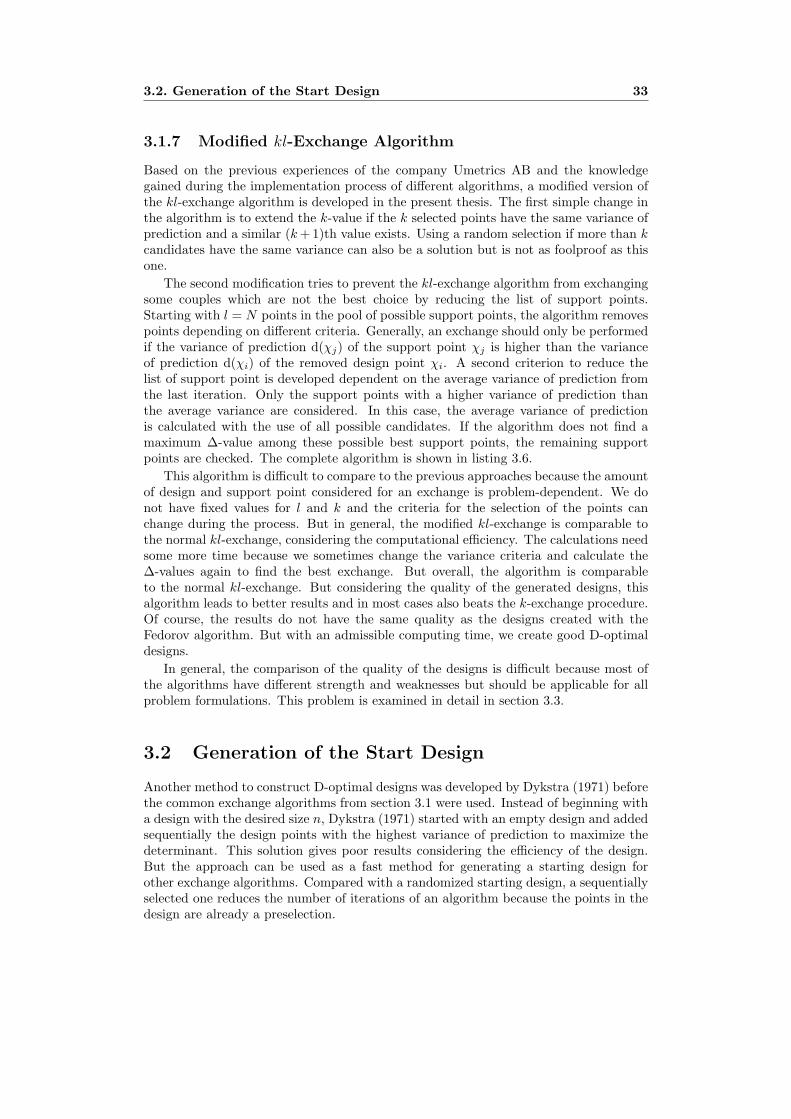
3.2. Generation of the Start Design 33
3.1.7 Modified kl-Exchange Algorithm
Based on the previous experiences of the company Umetrics AB and the knowledgegained during the implementation process of different algorithms, a modified version ofthe kl-exchange algorithm is developed in the present thesis. The first simple change inthe algorithm is to extend the k-value if the k selected points have the same variance ofprediction and a similar (k + 1)th value exists. Using a random selection if more than kcandidates have the same variance can also be a solution but is not as foolproof as thisone.
The second modification tries to prevent the kl-exchange algorithm from exchangingsome couples which are not the best choice by reducing the list of support points.Starting with l = N points in the pool of possible support points, the algorithm removespoints depending on different criteria. Generally, an exchange should only be performedif the variance of prediction d(χj) of the support point χj is higher than the varianceof prediction d(χi) of the removed design point χi. A second criterion to reduce thelist of support point is developed dependent on the average variance of prediction fromthe last iteration. Only the support points with a higher variance of prediction thanthe average variance are considered. In this case, the average variance of predictionis calculated with the use of all possible candidates. If the algorithm does not find amaximum ∆-value among these possible best support points, the remaining supportpoints are checked. The complete algorithm is shown in listing 3.6.
This algorithm is difficult to compare to the previous approaches because the amountof design and support point considered for an exchange is problem-dependent. We donot have fixed values for l and k and the criteria for the selection of the points canchange during the process. But in general, the modified kl-exchange is comparable tothe normal kl-exchange, considering the computational efficiency. The calculations needsome more time because we sometimes change the variance criteria and calculate the∆-values again to find the best exchange. But overall, the algorithm is comparableto the normal kl-exchange. But considering the quality of the generated designs, thisalgorithm leads to better results and in most cases also beats the k-exchange procedure.Of course, the results do not have the same quality as the designs created with theFedorov algorithm. But with an admissible computing time, we create good D-optimaldesigns.
In general, the comparison of the quality of the designs is difficult because most ofthe algorithms have different strength and weaknesses but should be applicable for allproblem formulations. This problem is examined in detail in section 3.3.
3.2 Generation of the Start Design
Another method to construct D-optimal designs was developed by Dykstra (1971) beforethe common exchange algorithms from section 3.1 were used. Instead of beginning witha design with the desired size n, Dykstra (1971) started with an empty design and addedsequentially the design points with the highest variance of prediction to maximize thedeterminant. This solution gives poor results considering the efficiency of the design.But the approach can be used as a fast method for generating a starting design forother exchange algorithms. Compared with a randomized starting design, a sequentiallyselected one reduces the number of iterations of an algorithm because the points in thedesign are already a preselection.

34 Chapter 3. D-Optimal Designs as a Computer Algorithm
create random design with desired number of points;while couples with positive delta are found do
calculate variance of prediction d(χi) for all design points;if more than k design points have same lowest variance of prediction then
extend given k;select k design points with lowest variance of prediction;calculate variance of prediction d(χj) for all support points;calculate average variance of prediction over whole candidate set;select l support points with higher variance of prediction than the averagevalue;for design point χ1 to design point χk do
calculate variance of prediction d(χi) for this design point;for support point χ1 to support point χl do
calculate variance of prediction d(χj) for this support point;if variance of the support point is higher than the variance of thedesign point then
calculate variance function d(χi, χj) for this couple;calculate delta function ∆(χi, χj) for this couple;check if maximum delta and save couple;
if maximum delta is negative thenselect N − l support points that have not been checked;for design point χ1 to design point χk do
calculate variance of prediction d(χi) for this design point;for support point χ1 to support point χN−l do
calculate variance of prediction d(χj) for this support point;calculate variance function d(χi, χj) for this couple;calculate delta function ∆(χi, χj) for this couple;check if maximum delta and save couple;
if maximum delta is positive thenif more then one couple with same maximum delta then
select couple randomly;exchange selected point χi with χj ;update information and dispersion matrix;reset maximum delta;
Algorithm 3.6: Modified kl-Exchange Algorithm.

3.3. Comparison of Exchange Algorithms 35
Galil & Kiefer (1980) used the idea of a sequential start design for Mitchell’s (1974)DETMAX algorithm and changed the start design to contain some random points in thebeginning. Thereafter, the design is sequentially filled with the best support points. Thenumber of the t random points was defined by Galil & Kiefer (1980) to be ‘considerablesmaller than k for moderate k [. . . ]’. Atkinson & Donev (1989) referred to this topic byusing a sequential start design for the kl-exchange algorithm. They defined the numberof random selected points t as a randomly chosen integer with the following condition:
0 ≤ t ≤ min([
12p
], N − 1
), (3.11)
where[12p
]denotes the integer part of the fraction and p is the number of used factors.
3.3 Comparison of Exchange Algorithms
Generally, a comparison of the algorithms has to be done depending on two main criteria.The first one is the used computing time to create a D-optimal design, and the secondone is the quality of the design. This quality or efficiency of the design can be evaluatedby the criteria taken from section 2.3. In this analysis we use the D-Optimality orits analog, the determinant to evaluate the optimal designs. Comparing other criteria,like the condition number or the G-Efficiency, can lead to other results than the onesshown in this section. The base for the given data in this comparison is an analysis ofthe four algorithms implemented at Umetrics AB. The case study was performed withan interaction model with 5, 7 or 9 factors. The software MODDE is used to createthe desired designs and calculates their efficiency, the logarithm of the determinant.During the calculation of 10 designs for each model and algorithm, the computing timeis measured and the mean value is calculated. The collected data can be found in table3.1.
5 factors 7 factors 9 factorstime/ms log(Det) time/ms log(Det) time/ms log(Det)
Fedorov 21.9 20.47 424.8 43.74 6887.2 75.33mod. Fedorov 21.8 20.47 286.7 43.74 3535.4 75.36k-exchange 10.9 20.47 84.6 43.71 669.2 74.83
mod. kl-exchange 20.3 20.47 126.6 43.72 931.7 74.99
Table 3.1: Comparison of Different Algorithms: This comparison is based on the imple-mented algorithms from chapter 4. Depending on an interaction model with five, sevenor nine factors, a set of ten designs has been created for each algorithm and model. Thecomputing time is the average value of the ten calculations and the efficiency is takenform the best of the designs. The best values of each column are printed in bold.
During the description of the algorithms in section 3.1, we show that some of themodifications are used to reduce the amount of calculations before an exchange is per-formed. The Fedorov algorithm, e.g., calculates the ∆-value for all possible couples andonly performs one exchange depending on this data. With a large number of factors,this approach is very expensive to use. The modified version by Cook & Nachtsheim(1980) reduces the number of calculations by performing up to n exchanges during each

36 Chapter 3. D-Optimal Designs as a Computer Algorithm
iteration and speeds up the algorithm by using more than one of the values. Table 3.1shows that the average computing time used for the modified Fedorov algorithm canbe up to 50% faster than the normal algorithm from 1972. Especially with large inputdata, the difference between the two algorithms becomes obviously. Other algorithms,like the k-exchange by Johnson & Nachtsheim (1983) or the modified kl-exchange, aremuch faster in the creation of D-optimal designs and can be used for huge numbers offactors. The k-exchange, e.g., can handle the interaction model with nine factors fromtable 3.1 ten-times faster than the basic Fedorov procedure. The Mitchell algorithm isnot implemented during the work of the present thesis but was studied and comparedby Johnson & Nachtsheim (1983). The evaluated data, depending on different modelsand factor setting, showed that the DETMAX algorithm has a computing time whichis comparable with the normal k-exchange.
Admittedly, a fast algorithm is not expedient if the created design has not the desiredquality or D-optimality. Hence, we have to compare the algorithms depending on thetime used and the quality of the created design. At this point we have to realize thatthe measured data from table 3.1 is difficult to evaluate. All of the algorithms can trapinto a so-called local optimum and stop the exchange process even if the best designis not found yet. With an increasing number of factors or model terms, the amountof local optima increases, too. Therefore, most of the D-optimal designs are differenteven if they rely on the same algorithm. In addition to this, the randomized functionsduring the selection process influence the outcome. Table 3.1 only shows the efficiencyof the best design out of ten generated possibilities. In general, it is recommended tocreate more than one design and to select the best one out of a pool of possible designs.The determinant of the information matrix (X ′X) for a small test, like the one in table3.1 with five factors, has the same value for all algorithms. In this case, it does notmatter which algorithm is used, they all create at least one design out of ten with thesame efficiency. If the number of factors increases or the model gets more complex,the Fedorov and modified Fedorov normally create the best designs, but in general, theselection of the best algorithm is problem-dependent. The modified kl-exchange, e.g.,creates better designs than the Fedorov or modified Fedorov in some cases or is at leastcomparable. Indeed, this algorithm is much faster than the Fedorov version and shouldbe preferred.
The findings from the above paragraph bear on the data presented in table 3.1 andadditional random samples. All of them are based on the implemented versions of thealgorithms inside the software MODDE. Therefore, this data is only an indicator thatleads to suppositions which algorithm should be used according to different aims. Inaddition to this, only the four implemented algorithms are considered. A comparisonof all algorithms under the same test condition does not exist in literature. Therefore,the selection of the four algorithms is based on two different comparisons. The first onewas performed by Cook & Nachtsheim (1980) and analyzes Mitchell’s (1974) DETMAX,the Fedorov procedure, the modified Fedorov procedure, the Wynn-Mitchell algorithm,and some other negligible algorithms. The conclusion of the article is that the bestdesigns are created with the Fedorov or modified Fedorov, but the Wynn-Mitchell al-gorithm should be used if a fast generation is more important. The second evaluationwas performed by Johnson & Nachtsheim (1983) and compared the Fedorov algorithm,the modified Fedorov algorithm, the k-exchange procedure, DETMAX ,and the Wynn-Mitchell algorithm. The outcome of this paper is the advice of the authors to use theWynn-Mitchell algorithm or its rough equivalent procedure, the k-exchange. Based onthese findings and the single publications of the algorithms, the four algorithms from

3.3. Comparison of Exchange Algorithms 37
table 3.1 are implemented in MODDE. Our small case study approves the advises fromJohnson & Nachtsheim (1983) and Cook & Nachtsheim (1980) but in order to havea reliable comparison, a separated complexity analysis has to be performed where allalgorithms are compared under the same criteria with the use of different problem for-mulations. But such an investigation goes beyond the limits of the present thesis.
Overall, the finding of the optimal combination of computing time and efficiency ofthe generated design is a difficult topic and cannot be concluded with a strict advicewhich algorithm to use. To sum up briefly, the modified Fedorov algorithm is similarto the normal Fedorov procedure if we consider the quality of the design but needsless computing time. Actually, both algorithms need a lot of calculations if the inputdata becomes big. Hence, for small designs the modified Fedorov algorithm by Cook &Nachtsheim (1980) should be used. For bigger designs the use of the simple k-exchangeor the modified kl-exchange is advisable. The created designs are a bit inferior in somecases, but with respect to the computing time this is the best choice. If the experimenterwants to create exact D-optimal designs and has the opportunity to evaluate a problemformulation with different algorithms and different parameters, this is the suggested wayto find the optimal design.
Generally, we discourage creating exact D-optimal designs because the selection ofthe right model is difficult and should be handled with care. To refer back to section 2.8,we repeat the same case study from table 3.1 with the use of a Bayesian modificationand try to confirm the findings from above. The addition of the potential terms makesthe designs more model-independent, and consequently the efficiency of the designs is abit below the ones created by the normal D-optimal process in table 3.1. A comparisonof both studies shows that the outstanding values follow the same regularity and provethe suggestions for the right algorithm selection.
5 factors 7 factors 9 factorstime/ms log(Det) time/ms log(Det) time/ms log(Det)
Fedorov 51.6 19.46 798.8 43.41 11343.4 74.66mod. Fedorov 35.8 19.46 295.6 43.41 4303.0 74.77k-exchange 21.9 19.46 129.5 43.16 915.5 74.32
mod. kl-exchange 31.3 19.46 215.7 42.71 1394.4 74.43
Table 3.2: Comparison of Different Algorithms (Bayesian Modification): This compar-ison belongs to the same case study as table 3.1, but the model matrix is extended withadditional potential terms to make the selected designs more model-independent.

38 Chapter 3. D-Optimal Designs as a Computer Algorithm
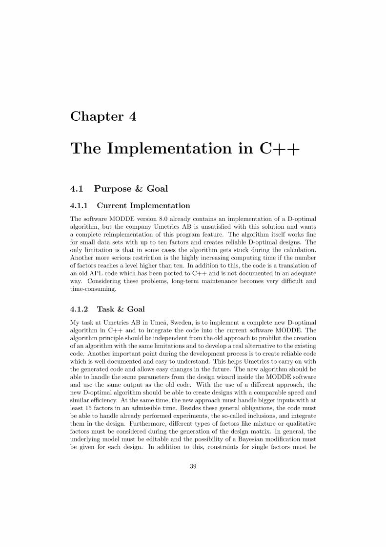
Chapter 4
The Implementation in C++
4.1 Purpose & Goal
4.1.1 Current Implementation
The software MODDE version 8.0 already contains an implementation of a D-optimalalgorithm, but the company Umetrics AB is unsatisfied with this solution and wantsa complete reimplementation of this program feature. The algorithm itself works finefor small data sets with up to ten factors and creates reliable D-optimal designs. Theonly limitation is that in some cases the algorithm gets stuck during the calculation.Another more serious restriction is the highly increasing computing time if the numberof factors reaches a level higher than ten. In addition to this, the code is a translation ofan old APL code which has been ported to C++ and is not documented in an adequateway. Considering these problems, long-term maintenance becomes very difficult andtime-consuming.
4.1.2 Task & Goal
My task at Umetrics AB in Umea, Sweden, is to implement a complete new D-optimalalgorithm in C++ and to integrate the code into the current software MODDE. Thealgorithm principle should be independent from the old approach to prohibit the creationof an algorithm with the same limitations and to develop a real alternative to the existingcode. Another important point during the development process is to create reliable codewhich is well documented and easy to understand. This helps Umetrics to carry on withthe generated code and allows easy changes in the future. The new algorithm should beable to handle the same parameters from the design wizard inside the MODDE softwareand use the same output as the old code. With the use of a different approach, thenew D-optimal algorithm should be able to create designs with a comparable speed andsimilar efficiency. At the same time, the new approach must handle bigger inputs with atleast 15 factors in an admissible time. Besides these general obligations, the code mustbe able to handle already performed experiments, the so-called inclusions, and integratethem in the design. Furthermore, different types of factors like mixture or qualitativefactors must be considered during the generation of the design matrix. In general, theunderlying model must be editable and the possibility of a Bayesian modification mustbe given for each design. In addition to this, constraints for single factors must be
39

40 Chapter 4. The Implementation in C++
considered and the calculation of the center-points has to be done before the design isshown on the worksheet. If more than one design is created, the possibility to select thedesign depending on the different optimal criteria has to be given in the design wizard.To sum up briefly, the requirements are:
1. Handling of more than 15 factors,
2. a computational efficiency which is comparable with the old implementation,
3. creation of designs which have a comparable optimality,
4. handling of the parameters from the design wizard,
5. output of the designs on the evaluation page and the worksheet of MODDE,
6. the possibility of a Bayesian modification must be given,
7. inclusion must be considered during the design generation,
8. the model must be editable,
9. mixture and qualitative factors must be handled,
10. center-point have to be added to the design,
11. and the code must be well structured and documented.
4.1.3 Preliminaries for a Reimplementation
Umetrics AB does not target the implementation of a certain algorithm. Therefore,an investigation of the different opportunities and a comparison of the approaches isnecessary before the implementation is started. Depending on the publications usedin chapter 3, the basic Fedorov algorithm is used for a preliminary investigation withMathWorks MATLAB. This analysis is used to get a basic overview about the generalexchange procedure and the necessary matrix calculations. The basis for this investi-gation are some MATLAB source files written by Ing-Marie Olsson from Umetrics AB.These files are independently developed from the current implementation in MODDE.In order to improve the knowledge about the D-optimal topic, the original files are re-coded, extended, and restructured to get acquainted with the whole D-optimal process.The modified files are used to test and investigate different D-optimal approaches andcalculations. Besides the Fedorov algorithm, the use of a Bayesian modification, the or-thogonal scaling, and the generation of the model-dependent design matrix are includedin this investigation. The revised files can be found in Appendix A.
4.2 Final Implementation
4.2.1 Input & Output
In MODDE the user can utilize the design wizard to create D-optimal designs with auser-friendly interface. The first step is the definition of the factors. Figure 4.1 shows ascreenshot of the wizard where the user has to define the factors, their types, and theirsettings. The possible options for the type and use of a factor are described in section1.2.3 and can be used to create, e.g., mixture designs. The settings are needed to define
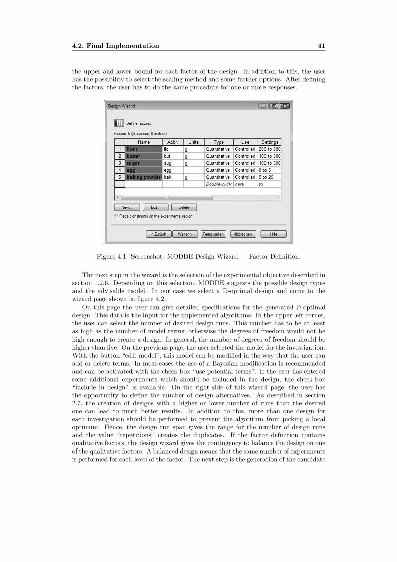
4.2. Final Implementation 41
the upper and lower bound for each factor of the design. In addition to this, the userhas the possibility to select the scaling method and some further options. After definingthe factors, the user has to do the same procedure for one or more responses.
Figure 4.1: Screenshot: MODDE Design Wizard — Factor Definition.
The next step in the wizard is the selection of the experimental objective described insection 1.2.6. Depending on this selection, MODDE suggests the possible design typesand the advisable model. In our case we select a D-optimal design and come to thewizard page shown in figure 4.2.
On this page the user can give detailed specifications for the generated D-optimaldesign. This data is the input for the implemented algorithms. In the upper left corner,the user can select the number of desired design runs. This number has to be at leastas high as the number of model terms; otherwise the degrees of freedom would not behigh enough to create a design. In general, the number of degrees of freedom should behigher than five. On the previous page, the user selected the model for the investigation.With the button “edit model”, this model can be modified in the way that the user canadd or delete terms. In most cases the use of a Bayesian modification is recommendedand can be activated with the check-box “use potential terms”. If the user has enteredsome additional experiments which should be included in the design, the check-box“include in design” is available. On the right side of this wizard page, the user hasthe opportunity to define the number of design alternatives. As described in section2.7, the creation of designs with a higher or lower number of runs than the desiredone can lead to much better results. In addition to this, more than one design foreach investigation should be performed to prevent the algorithm from picking a localoptimum. Hence, the design run span gives the range for the number of design runsand the value “repetitions” creates the duplicates. If the factor definition containsqualitative factors, the design wizard gives the contingency to balance the design on oneof the qualitative factors. A balanced design means that the same number of experimentsis performed for each level of the factor. The next step is the generation of the candidate

42 Chapter 4. The Implementation in C++
Figure 4.2: Screenshot: MODDE Design Wizard — D-Optimal Specification.
set. In general, MODDE creates the candidate set depending on the factor definitionand uses this data set for the calculation. Alternatively, the user can import an owncandidate set or edit the suggested one. The last group of options, in the bottom rightcorner, is new for the reimplementation of the D-optimal algorithm and gives the usermore options for the exchange procedure itself. The selection of the algorithm can bedone problem-dependent and additional parameters, like the k-value for the modifiedkl-exchange or the normal k-exchange by Cook & Nachtsheim (1980), can be defined.Normally, a sequential start design is recommended, but in some cases, the user needsthe opportunity to use the basic randomized start design to create other designs. Therandomized function can be used by deactivating the check-box “use sequential startdesign”. This features is explained in detail in section 4.2.5. The last option in thedesign wizard is the question if the user wants to have duplicated design points in thedesign or not. If this point is deactivated, the algorithm only considers the remainingsupport points for an exchange. In comparison to this, the use of duplicated design pointsinvokes a non-exhausting exchange procedure where all candidates are considered. Inthis case a design with replicated experiments is possible.
After all parameters are set, the algorithm is called and creates the desired numberof designs. The designs are listed on the next page of the wizard, shown in figure4.3. Depending on the four criteria: G-efficiency, the logarithm of the determinant, thenormalized logarithm of the determinant, and the condition number, the user has toselect the favored design.

4.2. Final Implementation 43
Figure 4.3: Screenshot: MODDE Design Wizard — Evaluation Page.
The selected design is printed out on the worksheet. Figure 4.4 shows an example ofa design with five factors. In general, the center-points and inclusions are part of thisdesign and placed in the first and last rows. The factors are unscaled and presented intheir normal range, as defined in the beginning of the design wizard.
Figure 4.4: Screenshot: MODDE Worksheet.
4.2.2 Integration & Program Flow
The core of the new D-optimal algorithm is placed in a class called newDopt with thesource file newDopt.cpp and the header file newDopt.h. The class name is chosen in thisway to implement the new code next to the existing version Dopt.cpp. The created filescan be found in Appendix A.
In general, the design wizard starts the creation of the D-optimal designs by call-ing the public function compute() of the class newDopt. This class itself is inheritedfrom the class design which is used inside MODDE for all design types. The param-eters and settings from the wizard are sent to the D-optimal algorithm inside the two

44 Chapter 4. The Implementation in C++
instances pModelSpec and pDOptSpec. The model specification contains detailed infor-mation about the factor constellation inside the model, the types of factors, and furtherinformation. The D-optimal specification contains the settings for the D-optimal algo-rithm, like the number of runs, the chosen algorithm, and so on. The general outline ofthe program flow can be seen in figure 4.5.
Figure 4.5: Program Flow I: This figure shows the general program flow of the newimplemented source code. With the specifications from the design wizard, the functioncompute() of the class newDopt is called. This function generates the extended modelmatrix and calls makeDopt() for each design. MakeDopt() selects the best design matrixwith an exchange algorithm and saves the design in the class DOptData.
The present thesis only deals with the algorithms to create D-optimal designs de-pending on an existing candidate set. Therefore, the generation of a new candidateset is implemented with a call of the old function generateCandidateSet(). This gener-ated candidate set and the specifications from the design wizard are the basis for thefollowing D-optimal algorithms. Depending on the model specification and the factorvalues in the candidate set, the first step is the generation of the model matrix for allcandidates. As described in section 2.2.2, the model matrix is a N × p matrix for all Ncandidates, where each of the p model terms is represented in one column. In general,this calculation can be easily done with the data provided in the model specificationand the simple candidate set. Only some special cases like mixtures or qualitative fac-tors should be handled cautiously. These special cases are explained in detail in section4.2.5. If the use of a Bayesian modification is selected in the design wizard, the modelmatrix is extended with the additional scaled potential terms. Which potential termshave to be added is model-dependent and is described in the following section. After themodification the model matrix contains all primary and potential model terms whichcan be used for the following calculations. Now, the function makeDopt() is called foreach of the desired designs. Depending on the given design run span and the numberof repetitions, the calculation is called until all designs are created. For each design,a new starting design is generated. The design can either be sequentially or randomly

4.2. Final Implementation 45
created depending on the selection in the design wizard. The start design is the basisfor the following exchange algorithm and should be different for each generation. Anexplanation of the implemented exchange algorithms follows later in this section. Oncethe generation of a D-optimal design is finished, the data is saved in the class DOptData,and the calculation for the next design is invoked. Inside DOptData the design matrixand the efficiency depending on different criteria are saved. The class DOptData is al-ready implemented in MODDE and therefore kept from the old implementation. Theclass is only modified to fit the requirements of the new approach. After all designs arecreated, the evaluation page of the design wizard pops up and lists the saved designs.After the selection by the user, the design is converted back into the unscaled data andprinted out on the worksheet.
Figure 4.6: Program Flow II: This picture shows the interaction between the normal useractivities inside the design wizard and the D-optimal generation process. The wizardstarts the generation, saves the designs in DoptData, and lists them in the evaluationpage. The selected design is printed out on the worksheet.
4.2.3 Variables
In order to find the optimal design matrix, different matrix calculations and exchangeprocedures are required. In this section we show the important member variables usedfor the calculation and define their types. Table 4.1 shows a list of these variables.
The class UmPointer is developed by Umetrics AB and represents a self- deallocatingpointer which can be used for different types of variables. The types FMatrix, FVector,and I2Vector belong to a math library used in MODDE, where F stands for float andI2 for integer. The keyword matrix is used for a multidimensional array with specialfunctionality for matrix multiplications or modifications. The vector class is similar tothis but has only one dimension.
As described in the first paragraph of this section, the specifications from the de-sign wizard are saved in two instances, one for the model information and one for theD-optimal settings. They have the names mpModelSpec and mpDOptSpec and are ac-cessible members in the whole newDopt class. An instance of the class DOptData is alsoimplemented as a member variable to save the created designs and make them availablefor the worksheet.
The generated candidate set is saved in two different ways. First, we have theunscaled data set, called mpUCS, taken as a float matrix from the existing code. Here,each factor represents one column and each candidate one row of the matrix. This is the
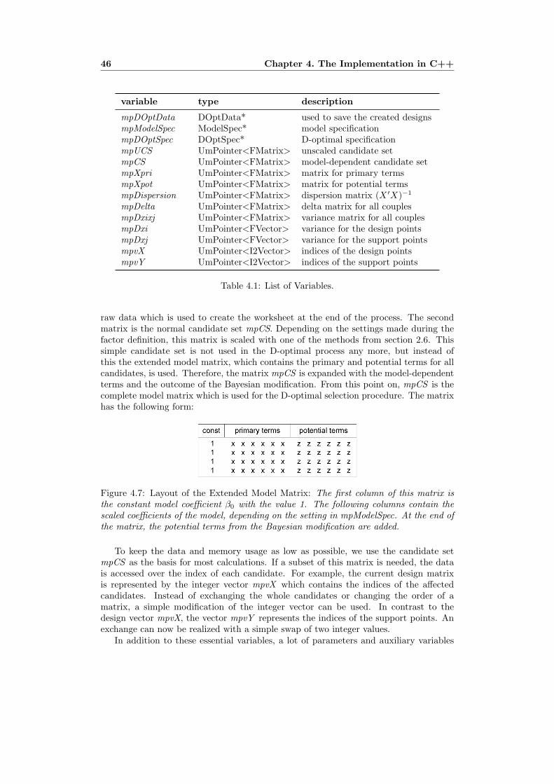
46 Chapter 4. The Implementation in C++
variable type description
mpDOptData DOptData* used to save the created designsmpModelSpec ModelSpec* model specificationmpDOptSpec DOptSpec* D-optimal specificationmpUCS UmPointer<FMatrix> unscaled candidate setmpCS UmPointer<FMatrix> model-dependent candidate setmpXpri UmPointer<FMatrix> matrix for primary termsmpXpot UmPointer<FMatrix> matrix for potential termsmpDispersion UmPointer<FMatrix> dispersion matrix (X ′X)−1
mpDelta UmPointer<FMatrix> delta matrix for all couplesmpDxixj UmPointer<FMatrix> variance matrix for all couplesmpDxi UmPointer<FVector> variance for the design pointsmpDxj UmPointer<FVector> variance for the support pointsmpvX UmPointer<I2Vector> indices of the design pointsmpvY UmPointer<I2Vector> indices of the support points
Table 4.1: List of Variables.
raw data which is used to create the worksheet at the end of the process. The secondmatrix is the normal candidate set mpCS. Depending on the settings made during thefactor definition, this matrix is scaled with one of the methods from section 2.6. Thissimple candidate set is not used in the D-optimal process any more, but instead ofthis the extended model matrix, which contains the primary and potential terms for allcandidates, is used. Therefore, the matrix mpCS is expanded with the model-dependentterms and the outcome of the Bayesian modification. From this point on, mpCS is thecomplete model matrix which is used for the D-optimal selection procedure. The matrixhas the following form:
Figure 4.7: Layout of the Extended Model Matrix: The first column of this matrix isthe constant model coefficient β0 with the value 1. The following columns contain thescaled coefficients of the model, depending on the setting in mpModelSpec. At the end ofthe matrix, the potential terms from the Bayesian modification are added.
To keep the data and memory usage as low as possible, we use the candidate setmpCS as the basis for most calculations. If a subset of this matrix is needed, the datais accessed over the index of each candidate. For example, the current design matrixis represented by the integer vector mpvX which contains the indices of the affectedcandidates. Instead of exchanging the whole candidates or changing the order of amatrix, a simple modification of the integer vector can be used. In contrast to thedesign vector mpvX, the vector mpvY represents the indices of the support points. Anexchange can now be realized with a simple swap of two integer values.
In addition to these essential variables, a lot of parameters and auxiliary variables

4.2. Final Implementation 47
are used in order to solve independent problems. These variables are explained whenthey are used to keep this section as compact as possible.
4.2.4 Exchange Algorithms
Depending on the findings from chapter 3, the following four exchange algorithms aresuggested for an implementation:
� Fedorov Algorithm,
� Modified Fedorov Algorithm,
� k-Exchange Algorithm,
� Modified kl-Exchange Algorithm.
The Fedorov algorithm from 1972 and its modified version by Cook & Nachtsheim(1980) showed the best results over all tests and should be used for small data sets.With an increasing number of factors, the k-exchange algorithm and the modified kl-exchange algorithm created comparable designs with a much higher computational effi-ciency. Hence, these two algorithms should be used for huge data sets.
The DETMAX algorithm by Mitchell (1974) and Johnson & Nachtsheim’s (1983)the basic kl-exchange algorithm are not considered for an implementation. The reasonfor this is the similarity in the created designs compared with the k-exchange algorithmand the modified kl-exchange algorithm. In addition to this, the DETMAX algorithmhas a complete different approach and is not familiar with the other solutions. Thefour selected algorithms can be implemented next to each other while using the samefundamentals like the calculation of the ∆-value or the exchange procedure.
Fedorov Algorithm
Depending on the calculated dispersion matrix (X ′X)−1, the function calculateDelta-Matrix() is called. Inside this function the necessary variance of prediction for thedesign and support points is calculated and the complete matrix of ∆-values is filledfor all possible couples. In addition to this, the indices of the suggested design andsupport points with the maximum ∆-value are saved in the member variables mixi andmixj. This data is used to start an exchange between the two integer vectors mpvX andmpvY. A swap of the values creates a new design matrix, and corresponding to this, thedispersion matrix has to be updated. This simple flow of actions is repeated until thefunction calculateDeltaMatrix() does not find a ∆-value bigger than mfepsilon. In thisimplementation the threshold value εfed is set to 10−6. The following listing shows theC++ routines for the Fedorov algorithm.
1 i f ( meAlgorithm == Fedorov )2 {3 // c a l c u l a t e d i s p e r s i on matrix (Xd ’*Xd)ˆ−1 fo r the f i r s t time4 ca l cu l a t eD i spe r s i onMat r i x ( ) ;5 // c a l c u l a t e the d e l t a va lue s f o r a l l coup l e s and f ind b i g g e s t6 ca l cu l a t eDe l taMat r ix ( ) ;7 // loop u n t i l no d e l t a b i g g e r e i s found8 while ( ( mfmaxdelta >= f e p s i l o n ) && ( icount < imaxloops ) ){9 // exchange the from ca l cu l a t eDe l t aMat r i x ( ) found coup le
10 exchangePoints ( mixi , mixj , mbal lowdubl icates ) ;11 //update the d i s p e r s i on matrix with the new poin t

48 Chapter 4. The Implementation in C++
12 updateDispers ionMatr ix ( mixi ) ;13 // c a l c u l a t e a l l d e l t a va lue s with the new d i s p e r s i on matrix14 ca l cu l a t eDe l taMat r i x ( ) ;15 }16 }
C++ Listing 4.1: Fedorov Algorithm.
Modified Fedorov Algorithm
Instead of implementing the modified Fedorov algorithm as an autonomous routine,the knowledge from section 3.1.5 is used. As Johnson & Nachtsheim (1983) noted, themodified Fedorov algorithm can be seen as a special case of the k-exchange procedure.Instead of considering k of the design points, the modified Fedorov algorithm checks alln points for a possible exchange. Based on this, the implementation can be done witha simple call of the normal k-exchange algorithm with k = n. Again, the procedure isshown in a C++ listing.
1 i f ( meAlgorithm == Modif iedFedorov )2 {3 mik = miruns ;4 meAlgorithm = KExchange ;5 }
C++ Listing 4.2: Modified Fedorov Algorithm.
k-Exchange Algorithm
The k-exchange is similar to the Fedorov procedure but only considers k of the designpoints for an exchange and performs up to k exchanges during each iteration. The algo-rithm also starts with the calculation of the dispersion matrix, but instead of calculatingthe ∆-values for all couples, the variance of prediction for the design points is calcu-lated. Depending on this float vector mpDxi, the indices of the k design points with thelowest variance of prediction are saved. The calculation of the variance vector and theevaluation is done inside the function calculateDxiVector(mik), where mik represents thek-value. The selected indices are saved in the integer vector mpvkListLow. Inside thefollowing loop shown in line 12 of listing 4.3, the ∆-values for the k points are calculated.In this case the function calculateDeltaRow(m) calculates the row of the ∆-matrix forthe corresponding candidate m, where m is one of the k considered design points. If asuggested exchange is found inside calculateDeltaRow(m), the corresponding couple isexchanged and the dispersion matrix has to be updated. If none of the k design pointscan be exchanged with a better point, the algorithm breaks. Otherwise, the selection ofk design points is started again.
1 i f ( meAlgorithm == KExchange )2 {3 // c a l c u l a t e d i s p e r s i on matrix (Xd ’*Xd)ˆ−1 fo r the f i r s t time4 ca l cu l a t eD i spe r s i onMat r i x ( ) ;5 // boo l va lue to check i f one o f the d e l t a s was p o s i t i v e (> f e p s i l o n )6 bool bposde l ta = fa l se ;7 while ( true ){
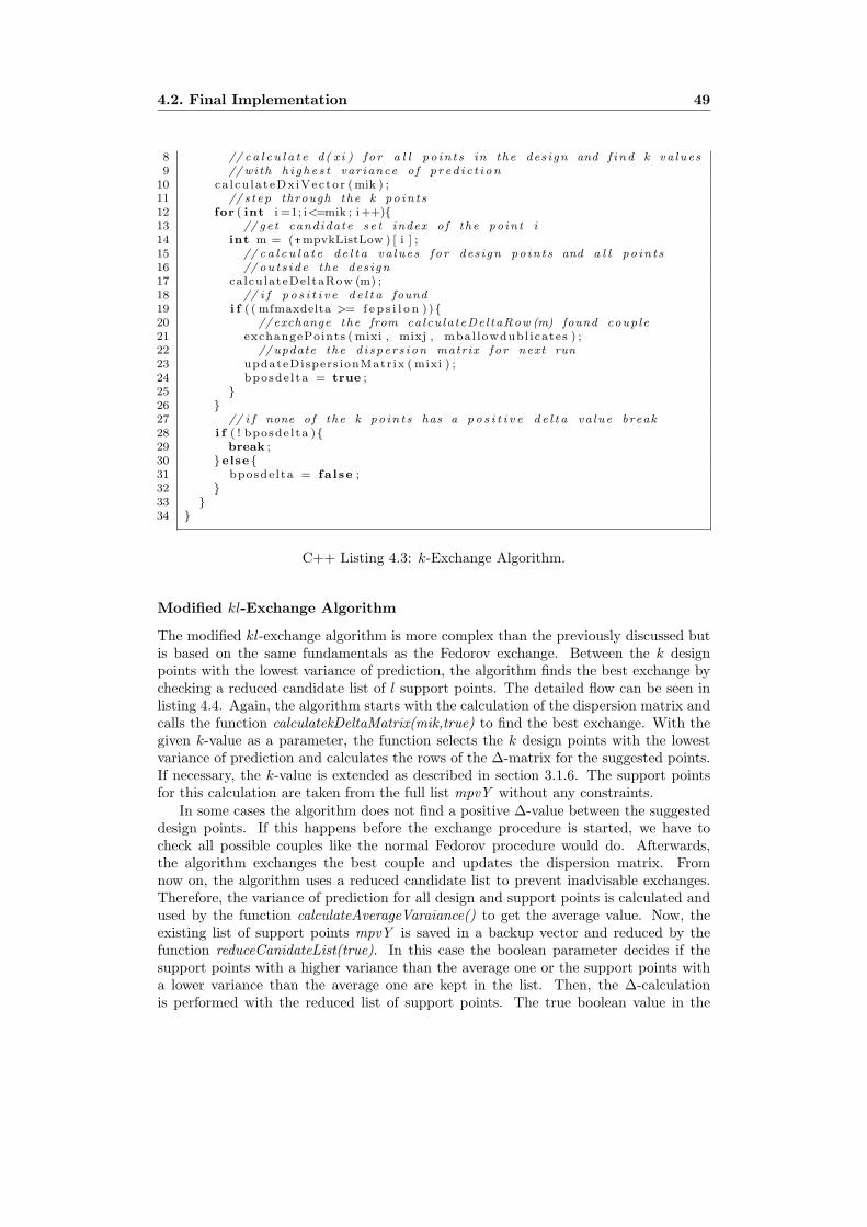
4.2. Final Implementation 49
8 // c a l c u l a t e d ( x i ) f o r a l l po in t s in the des ign and f ind k va lue s9 //with h i g h e s t var iance o f p r ed i c t i on
10 ca l cu la t eDx iVec to r (mik ) ;11 // s t ep through the k po in t s12 for ( int i =1; i<=mik ; i++){13 // ge t candidate s e t index o f the po in t i14 int m = (*mpvkListLow ) [ i ] ;15 // c a l c u l a t e d e l t a va lue s f o r des ign po in t s and a l l po in t s16 // ou t s i d e the des ign17 calculateDeltaRow (m) ;18 // i f p o s i t i v e d e l t a found19 i f ( ( mfmaxdelta >= f e p s i l o n ) ){20 // exchange the from calcu la teDel taRow (m) found coup le21 exchangePoints ( mixi , mixj , mbal lowdubl icates ) ;22 //update the d i s p e r s i on matrix f o r next run23 updateDispers ionMatr ix ( mixi ) ;24 bposde l ta = true ;25 }26 }27 // i f none o f the k po in t s has a p o s i t i v e d e l t a va lue break28 i f ( ! bposde l ta ){29 break ;30 } else {31 bposde l ta = fa l se ;32 }33 }34 }
C++ Listing 4.3: k-Exchange Algorithm.
Modified kl-Exchange Algorithm
The modified kl-exchange algorithm is more complex than the previously discussed butis based on the same fundamentals as the Fedorov exchange. Between the k designpoints with the lowest variance of prediction, the algorithm finds the best exchange bychecking a reduced candidate list of l support points. The detailed flow can be seen inlisting 4.4. Again, the algorithm starts with the calculation of the dispersion matrix andcalls the function calculatekDeltaMatrix(mik,true) to find the best exchange. With thegiven k-value as a parameter, the function selects the k design points with the lowestvariance of prediction and calculates the rows of the ∆-matrix for the suggested points.If necessary, the k-value is extended as described in section 3.1.6. The support pointsfor this calculation are taken from the full list mpvY without any constraints.
In some cases the algorithm does not find a positive ∆-value between the suggesteddesign points. If this happens before the exchange procedure is started, we have tocheck all possible couples like the normal Fedorov procedure would do. Afterwards,the algorithm exchanges the best couple and updates the dispersion matrix. Fromnow on, the algorithm uses a reduced candidate list to prevent inadvisable exchanges.Therefore, the variance of prediction for all design and support points is calculated andused by the function calculateAverageVaraiance() to get the average value. Now, theexisting list of support points mpvY is saved in a backup vector and reduced by thefunction reduceCanidateList(true). In this case the boolean parameter decides if thesupport points with a higher variance than the average one or the support points witha lower variance than the average one are kept in the list. Then, the ∆-calculationis performed with the reduced list of support points. The true boolean value in the

50 Chapter 4. The Implementation in C++
function call calculatekDeltaMatrix(mik,true) achieves a second variance check duringthe ∆-calculation. Only couples whose support point has a higher variance of predictionthan the design point are considered for an exchange.
If no positive ∆-value is found during this check, the algorithm switches the listmpvY by restoring the old list and calling the function reduceCanidateList(false) whichselects only the points with a variance of prediction less or equal the average one. Thefunction calculatekDeltaMatrix(mik,false) is called without a variance check and findsthe best possible exchange. Afterwards, the list of support points is restored and thenext iteration begins. If the whole process does not find a positive ∆, the algorithmbreaks.
1 i f ( meAlgorithm == ModifiedKLExchange )2 {3 // average var iance o f p r ed i c t i on over the whole candidate s e t4 mfavVar=0.0 ;5 // va lue and id o f the l a s t exchanged po in t to prevent a6 // reve r s e exchange7 mi l a s t exva l = 0 ;8 m i l a s t ex id = 0 ;9 // c a l c u l a t e the d i s p e r s i on matrix (Xd ’ * Xd)ˆ−1 fo r the f i r s t time
10 ca l cu l a t eD i spe r s i onMat r i x ( ) ;11 // c a l c u l a t e the d e l t a va lue s f o r the k des ign po in t s ( var iance o f12 // the candidate > var iance o f des ign po in t ) and f ind b i g g e s t d e l t a13 ca l cu la t ekDe l taMatr ix (mik , true ) ;14 // i f no max d e l t a i s found during the k des ign po in t s check again15 // fo r a l l po in t s ( k=miruns , no var iance c r i t e r i a )16 i f ( mfmaxdelta<f e p s i l o n ){17 ca l cu la t ekDe l taMatr ix ( miruns , fa l se ) ;18 }19 // loop wh i l e p o s i t i v e d e l t a s are found20 while ( ( mfmaxdelta >= f e p s i l o n ) && ( icount < imaxloops ) ){21 // exchange the from ca l cu l a t e kDe l t aMat r i x ( ) found coup le22 exchangePoints ( mixi , mixj , mbal lowdubl icates ) ;23 //update the d i s p e r s i on matrix (Xd ’*Xd)ˆ−124 updateDispers ionMatr ix ( mixi ) ;25 // c a l c u l a t e the vec tor with the d ( x j ) and d( x i ) func t i on26 // ( var iance o f p r ed i c t i on ) and ge t the average var iance27 // o f t he se v e c t o r s28 ca l cu la t eDxjVecto r ( ) ;29 ca l cu la t eDx iVec to r ( ) ;30 ca l cu lateAverageVara iance ( ) ;31 // save the l i s t o f cand ida tes (mpvY) and crea t e a reduced32 // the l i s t to speed up the a lgor i thm . the reduced l i s t33 // conta ins only the po in t t ha t have a var iance o f p r ed i c t i on34 //> the average one from the l a s t i t e r a t i o n35 saveCanidateL i s t ( ) ;36 reduceCanidateL i s t ( true ) ;37 // fo r the next run : c a l c u l a t e the d e l t a va lue s f o r the k des ign38 // po in t s ( var iance o f the candidate > var iance o f des ign po in t )39 //and f ind b i g g e s t d e l t a40 ca l cu la t ekDe l taMatr ix (mik , true ) ;41 // r e s t o r e the be f o r e saved candidate s e t (mpvY)42 r e s t o r eCan ida t eL i s t ( ) ;43 // i f no max d e l t a was found in the reduced candidate se t , take44 // the cand ida tes t ha t haven ’ t been cons idered in the45 // i n v e s t i g a t i on , c a l c u l a t e the d e l t a s and r e s t o r e the candidate46 // s e t (no var iance c r i t e r i a )47 i f ( mfmaxdelta<f e p s i l o n ){48 reduceCanidateL i s t ( fa l se ) ;

4.2. Final Implementation 51
49 ca l cu la t ekDe l taMatr ix (mik , fa l se ) ;50 r e s t o r eCan ida t eL i s t ( ) ;51 }52 }53 }
C++ Listing 4.4: Modified kl-Exchange Algorithm.
Delta-Calculation
All of the four algorithm call a slightly different function to calculate the needed ∆-values. Listing 4.5 shows, e.g., the function calculateDeltaMatrix() which is used by theFedorov algorithm. The function calculates the variance of prediction of the design andthe support points with the functions calculateDxiVector() and calculateDxjVector() anduses this data to calculate the ∆-values for all possible couples. The values are savedin the matrix mpDelta and the coordinates of the couple with the biggest ∆-value aresaved in mixi and mixj.
1 void newDopt : : ca l cu l a t eDe l taMat r ix ( )2 // c a l c u l a t e a l l d e l t a va lue s f o r a l l po in t s in the des ign3 {4 // r e s e t i d s o f p o s s i b l e exchange points , r e s e t maxdelta5 mixi = 0 ;6 mixj = 0 ;7 mfmaxdelta = −99.9;8 // ge t d ( x i ) vec to r f o r des ign po in t s9 ca l cu la t eDx iVecto r ( ) ;
10 // ge t d ( x j ) vec to r f o r support po in t s11 ca l cu la t eDxjVecto r ( ) ;12 // s t ep through a l l coup l e s o f x i and x j and c a l c u l a t e t h e i r d e l t a s13 for ( int i = 1+miInc l ; i<=miruns ; i++){14 for ( int j = 1 ; j<=mpvY−>NVal ( ) ; j++){15 // ge t d ( xi , x j ) f o r t h i s coup le16 (*mpDxixj ) [ i ] [ j ]= ca l cu l a t eDx i x j ( i , j ) ;17 // ge t d e l t a ( xi , x j ) f o r t h i s coup le18 (*mpDelta ) [ i ] [ j ]= ca l c u l a t eDe l t a ( i , j ) ;19 // check i f t h i s d e l t a i s maximum and save coord ina te s20 i f ( (*mpDelta ) [ i ] [ j ]>mfmaxdelta ){21 mfmaxdelta = (*mpDelta ) [ i ] [ j ] ;22 mixi = i ;23 mixj = j ;24 }25 }26 }27 }
C++ Listing 4.5: Function: calculateDeltaMatrix().
The other implemented algorithms have similar solutions but the number of consideredcouples is smaller. The data is also saved inside mpDelta even if not all storage positionsof the array are used. The connection between the candidate set mpCS, the design vectormpvX, the support vector mpvY, the variance vectors mpDxi and mpDxj, and the ∆-matrix mpDelta is shown in figure 4.8. The current design is realized by the use of theindices of the candidates. Each of these candidates has a variance of prediction whichis saved in mpDxi or mpDxj. These float values are also connected by the indices of the

52 Chapter 4. The Implementation in C++
candidates. The ∆-matrix mpDelta combines the design and support points to couplesand uses the corresponding variances for the calculation.
Figure 4.8: Use of Indices to Calculate the Delta-Matrix: This picture shows the con-nection between the candidate set, the design vectors, and the ∆-matrix. The vectors Xand Y contain the indices of the candidate points which are currently in the design Xor in the list of support points Y. The arrow show an example how the ∆-value for thecouple (6,7) is calculated.
4.2.5 Features
Besides the normal exchange procedure, the implementation of the D-optimal processintegrates some additional features. Those features also have been implemented in theold version but are completely new implemented in the present thesis. In this sectionsome of them are explained in detail, and in some cases the used C++ source code isprovided and outlined to clarify the approach.
Inclusions
An inclusion is an already performed experiment which should be integrated into theoptimal design matrix. Theses experiments are entered by the user and have to bepresent in the created worksheet. Therefore, theses candidates have to be consideredduring the generation of the start design and during the exchange procedure. Lettingo be the number of included candidates, the easiest way is to place the inclusions ontop of the candidate set and handle the following calculations with an offset of o points.This means, when the starting design is generated the first o points are taken from thecandidate set followed by the randomly or sequentially included points. The exchangeprocedure works with the same concept. For the first o candidates no ∆ is calculatedand therefore, the points are not considered for an exchange. Attention should be paidto the calculation of the dispersion matrix and efficiency. Here, the inclusions have tobe considered because they are part of the evaluated design. Table 4.9 shows a simpleexample of a candidate set with inclusions and center-points. In this implementationthe integer variable miIncl contains the offset value.

4.2. Final Implementation 53
Figure 4.9: Layout of the Candidate Set: The candidate set contains the inclusions in thefirst rows. These candidates will not be exchanged and are present in the final worksheet.All following candidates are normal support points. The last row of the matrix is thecenter-point.
Center-Points
A center-point is a candidate which has the mean value of the upper and lower bounds ofeach factor definition as a value. Above all, we have to differentiate between two differentapplications of center-points. On the one hand, we have the additional center-pointswhich are normally used to test the robustness of an already created D-optimal design.Therefore, the additional center-points, normally three, are not considered during thenormal exchange procedure and they are added after the generation. On the other hand,one center-point is included in the candidate set as a possible candidate. This candidateis handled like a normal support point and is considered during the start design and theexchange process. In order to keep the candidate set clear, the center-point is normallyadded in the last row. This makes the selection of the additional center-points easy andthe candidate can be used as a normal support point. The placement of the center-pointcan also be seen in figure 4.9. To add the robustness testing center-point to the finaldesign, the function addCentroids() is called. Here, the design matrix is expanded withthe desired number of center-points taken from the last row of the unscaled candidateset mpUCS.
Bayesian Modification
The Bayesian modification, described in section 2.8, is realized by a call of the functionaddPotentialTerms(). Inside this function the matrix with the primary terms Xpri isanalyzed, and depending on the model and the factor definitions, the potential termsfrom table 4.2 are added to the matrix Xpot.
After the creation of the matrix, the Bayesian scaling is applied. Listing 4.6 shows theC++ code of the scaling procedure implemented in the function doBayesianScaling().The first step is to calculate the α-matrix which contains the least square coefficientsof Xpot on Xpri. Depending on this calculation, the residual of the regression is savedin the matrix R. The matrix calculations are solved with the math library of MODDE.The needed column-wise maximum and minimum values of R can easily be extracted asa float vector by the use of the class FMatrix. These two float vectors, Rmax and Rmin,are used for the final calculation of the Z-matrix mpZ which is defined in equation2.32 of section 2.8.2. In order to finish the Bayesian modification, the new Z-matrixis attached to the candidate set with the function updateCS(). In general, the τ -valuein this implementation is set to one. With this default the Q-matrix is a simple diag-

54 Chapter 4. The Implementation in C++
modelprocess factors mixture factorscount potential terms count potential terms
linear all interactions up to 20 all interactionsall squaresa,b up to 20 all squares
interation missing interactionsall squaresa,b
quadratic
missing squaresall interactions
up to 10 all cubesb up to 12 all cubesup to 6 all three-way inter. up to 6 all three-way inter.
special cubic up to 6 all three-way inter.
cubic up to 6 all three-way inter.a only included if no interaction terms are added or the model contains a square valueb factor must be quantitative or multilevel
Table 4.2: List of Potential Terms: This table shows the selection of the potential termsbased on the assumed model and the type of the used factors. We differentiate betweenprocess and mixture factors in general. Depending on the amount of factors, differentpotential terms are added to the matrix.
onal matrix with ones in the diagonal if the column belongs to a potential term. Thesimple construction of this matrix is shown in listing 4.7. During the calculation of thedispersion matrix, this matrix is considered, as shown in equation 2.34.
1 void newDopt : : doBayes ianSca l ing ( )2 // alpha = (Xpri ’ * Xpri)ˆ−1 * Xpri ’ * Xpot3 //R = Xpot − (Xpri * alpha )4 //Z = R / (max(R) −min(R))5 {6 // c a l c u l a t e the needed transpose o f Xpri7 for ( int j = 1 ; j<=mpXpri−>NRow( ) ; j++){8 for ( int k = 1 ; k<=mpXpri−>NCol ( ) ; k++){9 (*mpXpriT ) [ k ] [ j ] = (*mpXpri ) [ j ] [ k ] ;
10 }11 }12 // c a l c u l a t e a lpha13 mpAlpha . r e s e t (new FMatrix ( (*mpXpriT)* (*mpXpri ) ) ) ;14 mpAlpha−>MInv ( ) ;15 (*mpAlpha) = ((*mpAlpha )* (*mpXpriT ) )* (*mpXpot ) ;16 // c a l c u l a t e R17 mpR. r e s e t (new FMatrix ( (*mpXpot) − ( (*mpXpri )* (*mpAlpha ) ) ) ) ;18 // ge t max o f each column of R19 FVector Rmax = mpR−>MaxCol ( ) ;20 // ge t min o f each column of R21 FVector Rmin = mpR−>MinCol ( ) ;22 // c a l c u l a t e Z23 mpZ. r e s e t (new FMatrix (mpR−>NRow( ) ,mpR−>NCol ( ) , 0 . 0 , 1 ) ) ;24 for ( int i =1; i<=mpR−>NRow( ) ; i++){25 for ( int j =1; j<=mpR−>NCol ( ) ; j++){26 (*mpZ) [ i ] [ j ] = (*mpR) [ i ] [ j ] / (Rmax[ j ]−Rmin [ j ] ) ;27 }28 }

4.2. Final Implementation 55
29 }
C++ Listing 4.6: Function: doBayesianScaling().
1 void newDopt : : createQ ( )2 // c r ea t e s a matrix with ones in the d iagona l i f the column3 // be longs to a p o t e n t i a l term4 {5 // square matrix6 mpQ. r e s e t (new FMatrix ( micols , micols , 0 . 0 , 1 ) ) ;7 // fo r p o t e n t i a l terms add ones in the diagonal ,8 // a l l o the r s are zeros9 for ( int i=miprimterms+1; i <=(miprimterms+mipotterms ) ; i++){
10 (*mpQ) [ i ] [ i ]=1;11 }12 }
C++ Listing 4.7: Function: createQ().
Duplicated Design Points
The previous chapters explains the difference between an exhausting and a non-exhaustingsearch method for the selection of the support points. Because of different aims duringthe generation of a design, the implementation gives the user the possibility to selectwhether duplicated points should be avoided or not. The default option is not to useduplicated experiments. The two main differences between the approaches can be seenduring the creation of the start design and the exchange procedure. If no duplicated ex-periments are allowed, the start design is generated by picking the points out of a list ofthe remaining support points. With allowing repeated experiments, the support pointsare selected from the full set of candidate points. During the exchange procedure thevector of support points mpvY contains either the remaining candidates which are notconsidered in the current design or the full candidate set. If an exchange is performed,normally both points from the design vector mpvX and the support vector mpvY areexchanged. But if duplicated points are allowed in the design, the support vectors mustnot be changed. Only the design is updated with a new point. Listing 4.8 shows thefunction which is used to perform an exchange.
1 void newDopt : : exchangePoints ( int xi , int xj , bool bdub l i c a t e s )2 // exchanges two po in t s ( des ign po in t from X with support po in t3 //from Y)4 {5 // save the exchange to prevent r eve r s e exchange6 mi l a s t exva l = (*mpvX) [ x i ] ;7 m i l a s t ex id = x i ;8 // exchange the po in t x i from X with the po in t from Y9 i f ( ! bdub l i c a t e s ){
10 int temp = (*mpvY) [ x j ] ;11 (*mpvY) [ x j ]=(*mpvX) [ x i ] ;12 (*mpvX) [ x i ]=temp ;13 // i f d u p l i c a t e s are al lowed , j u s t copy the candidate14 // in to the des ign wi thout changing Y15 } else {16 (*mpvX) [ x i ]=(*mpvY) [ x j ] ;

56 Chapter 4. The Implementation in C++
17 }18 }
C++ Listing 4.8: Function: exchangePoints( int xi, int xj, bool bdublicates).
If the option “allow duplicated points” is activated in the design wizard, we haveto consider two checks to avoid problems during the design creation. First, we have tocheck if the entered inclusions are already parts of the candidate set. In this case wehave to delete one of the duplicated experiments. The second check is performed toexamine if the selected number of design runs is higher than the amount of candidates.This means that the number of support points must be high enough to fill the startingdesign with the desired number of runs. If this is not possible, the user must considerduplicated experiments in the design or add further candidates.
Start Design
The randomized start design is based on a repeated exchange process between the designvector mpvX and the vector of support points mpvY. Instead of just shuffling a list ofpoints, the use of the exchange procedure can handle the duplicated option, mentionedabove. First, the list of design points is filled continuously with candidates until thenumber of desired runs is reached. Then, the list of support points is initialized withthe remaining points or with all candidates depending on the option in the wizard. Theexchange procedure now randomly generates indices for both lists and takes care of theexchanges. During this process the fixed inclusions in the first rows of the start designare considered.
If we use the sequential start design, as described in section 3.2, the randomized de-sign can be used as a basis for the generation process. The design consists of three typesof support points which are added consecutively. The first group are the o inclusionswhich have to be in each design. These points are followed by q randomized points,where the integer q itself is a randomized number. The missing n− o− q design pointsare chosen from the list of support points to increase the determinant most. Figure 4.10shows the layout of the sequential start design.
Figure 4.10: Layout of the Sequential Start Design: This table shows the general struc-ture of a sequential start design. The inclusions and random points are taken from arandomized design. The missing support points are added depending on their varianceof prediction.

4.2. Final Implementation 57
With an already generated randomized design with the o inclusions in the first row,the first o + q design point can be used for the selection process of the first additionalpoint. The dispersion matrix of the design with these points has to be calculated, andcorresponding to this, the point with the highest variance of prediction can be foundand added to the design. This process is repeated until the desired number of designruns is reached. The source code for the creation of both start designs can be found inappendix A.
Mixture Factors
In order to handle mixture designs, the candidate set is modified by removing one of thefactor definitions. Considering, e.g., a design with three mixture factors, we only need toperform the D-optimal process with two of the definitions because they sum up to 100%and therefore the missing factors can be calculated after the exchange procedure. If thefactors have the values a=0.3 and b=0.5, consequently the factor c must be equal to 0.2.This modification speeds up the algorithm, but the excluded factor has to be consideredduring the creation of the primary and potential terms. To handle this problem, theindex of the factor is saved in the variable miexclfactor. Each term is checked if itcontains the excluded factor and if needed the indices are fixed inside the functionsaddPrimaryTerms() and addPotentialTerms().
Qualitative and Quantitative Factors
Qualitative factors have at least two discrete values and can also be used in D-optimaldesigns. Inside the candidate set these factors are represented in distinct columns de-pending on the number of levels. This means the data is displayed in a binary codingwhere x columns can represent 2x discrete values. A qualitative factor with, e.g., threelevels A, B and C uses two columns to represent the data in a valuable way. Table4.3 shows the number of needed columns for different factor levels. Building the modelmatrix depending on the normal model specification is difficult because each of the qual-itative factors each has an expanded count. With the use of offset values this problemis also solved in the functions addPrimaryTerms() and addPotentialTerms().
Levels Columns
2 13-4 25-8 39-16 4
Table 4.3: Columns Needed to Handle Qualitative Factors.
Balanced Designs
Using the qualitative factors mentioned above, the user has the opportunity to use theD-optimal process only for the creation of balanced designs. These designs contain thesame number of experiments for each level of a qualitative factor. Considering, e.g., adesign with a qualitative factor which has three discrete values A, B, and C, a balanceddesign with n = 12 runs contains four experiments with value A, four with value B,

58 Chapter 4. The Implementation in C++
and four with value C. The exchange procedure of the D-optimal algorithms does notautomatically create balanced designs, but with the function IsBalanced(PtrI2VectorpDesignN, std::map<int,int>*pBalancedQualSetting) a generated design vector can beanalyzed. If the option “use balanced only” is activated in the design wizard, theevaluation page only shows the created designs which fulfill the balancing criteria. Inorder to avoid the calculation of design which cannot be balanced due to their numberof runs, a check before the call of the function makeDopt() is performed. A design witha desired number of runs which is not a multiple of the amount of discrete factor valuescannot be balanced. In our example above, only designs with n = z ∗ 3 design runs canbe balanced. If more than one qualitative factor is used in the design, the user has toselect the one to balance on in the wizard. The number of discrete values and the indexof the factor is saved in the variable std::map<int,int>*pBalancedQualSetting which isused for the verification of the designs.
Irregular Experimental Region
An irregular experimental region can be handled with the D-optimal implementationlike a normal symmetrical area. Instead of a candidate set which uses the upper andlower bounds of each factor, the defined constraints are used to change the candidateset. Depending on this changed candidates, the D-optimal algorithm performs a normalexchange until the optimal design matrix is found.
Chapter 5
Summary & Conclusions
5.1 Summary
The aim of the present thesis is the development and documentation of a D-optimalprocess to create designs which fulfill different criteria. In Chapter 1 and 2, the basicprinciples and the need for such D-optimal designs are shown and exemplified. With theuse of the model concept and simple statistical design, the reader has the opportunity toget started with the concept of DoE. We clarify that normal designs are not applicablein situations with, e.g., an irregular experimental region or when already performedexperiments have to be included in the design. To take up our example from the prefacein chapter 1, the baking of a cake can now be analyzed with the use of DoE, e.g., witha full factorial design. To expand this problem formulation for a D-optimal design, wesimply have to consider some recipes of already baked cakes which have to be includedin the design.
The D-optimal process is used to select the optimal combination of experimentsout of all possible designs. This selection process depends on the given criteria fromsection 2.3 and is solved by a computer algorithm. A goal before the implementationcan be started is the selection of a suitable exchange algorithm. Chapter 3 deals withthis topic and explains and analyses six different algorithms which differentiate in thecomputational efficiency and the quality of the created designs. The outcome of thiscomparison is the implementation of four different algorithms, the Fedorov algorithm,the modified Fedorov algorithm, the k-exchange algorithm, and the modified kl-exchangealgorithm. All of these exchange approaches are problem-dependent, and therefore thechoice of only one algorithm to fulfill all requirements is impossible. The implementedFedorov and modified Fedorov algorithm create the best designs considering the D-optimality but are very time-consuming. Therefore, the k-exchange should be applied ifthe number of factors reaches a level of 10 or more. In this case the Fedorov algorithmis also adaptable, but the calculation needs much time. Considering the advice tocreate more than one design and select the best one, the k-exchange creates normallycomparable result. In some cases the k-exchange algorithm shows weakness when, e.g.,more than k design points have the same lowest variance of prediction. To avoid this, themodified kl-exchange algorithm developed during the present thesis should be applied.In general, this approach needs a longer computing time than the k-exchange algorithmbut generates better results for huge data sets with, e.g., 15 factors. Overall, the advicewhich algorithm to use is difficult and one of the reasons why up to four of the algorithms
59
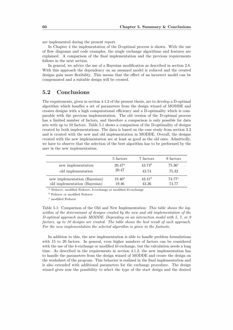
60 Chapter 5. Summary & Conclusions
are implemented during the present report.In Chapter 4 the implementation of the D-optimal process is shown. With the use
of flow diagrams and code examples, the single exchange algorithms and features areexplained. A comparison of the final implementation and the previous requirementsfollows in the next section.
In general, we advice the use of a Bayesian modification as described in section 2.8.With this approach the dependency on an assumed model is reduced and the createddesigns gain more flexibility. This means that the effect of an incorrect model can becompensated and a suitable design will be created.
5.2 Conclusions
The requirements, given in section 4.1.2 of the present thesis, are to develop a D-optimalalgorithm which handles a set of parameters from the design wizard of MODDE andcreates designs with a high computational efficiency and a D-optimality which is com-parable with the previous implementation. The old version of the D-optimal processhas a limited number of factors, and therefore a comparison is only possible for datasets with up to 10 factors. Table 5.1 shows a comparison of the D-optimality of designscreated by both implementations. The data is based on the case study from section 3.3and is created with the new and old implementation in MODDE. Overall, the designscreated with the new implementation are at least as good as the old ones. Admittedly,we have to observe that the selection of the best algorithm has to be performed by theuser in the new implementation.
5 factors 7 factors 9 factors
new implementation 20.47a 43.74b 75.36c
old implementation 20.47 43.74 75.32
new implementation (Bayesian) 19.46a 43.41b 74.77c
old implementation (Bayesian) 19.46 43.36 74.77a Fedorov, modified Fedorov, k-exchange or modified kl-exchangeb Fedorov or modified Fedorovc modified Fedorov
Table 5.1: Comparison of the Old and New Implementation: This table shows the log-arithm of the determinant of designs created by the new and old implementation of theD-optimal approach inside MODDE. Depending on an interaction model with 5, 7, or 9factors, up to 10 designs are created. The table shows the best result of each approach.For the new implementation the selected algorithm is given in the footnote.
In addition to this, the new implementation is able to handle problem formulationswith 15 to 20 factors. In general, even higher numbers of factors can be consideredwith the use of the k-exchange or modified kl-exchange, but the calculation needs a longtime. As described in the requirements in section 4.1.2, the new implementation hasto handle the parameters from the design wizard of MODDE and create the design onthe worksheet of the program. This behavior is realized in the final implementation andis also extended with additional parameters for the exchange procedure. The designwizard gives now the possibility to select the type of the start design and the desired
5.3. Limitations 61
algorithm and allows selecting if duplicated support points should be considered. Duringthe selection process the application of a Bayesian modification is possible. The addi-tional features demanded by Umetrics AB like handling of inclusions, mixture designs,quantitative factors et cetera are all implemented and explained in detail in section 4.2.5of the present thesis.
5.3 Limitations
The developed D-optimal process has no real limitations considering the requirementsfrom section 4.1.2. But during the testing of the algorithm one weakness of the modifiedkl-exchange was found. The algorithm is not able to handle designs which have a toolow number of degrees of freedom. If the number is below five, the created designs havea weak D-optimality and should not be used. In this case, the use of another algorithmis advised. In general, the design wizard warns the user for all four algorithms if thenumber of degrees of freedom is below five and designs should not be created underthese conditions, even if the other algorithms can handle the problem. To avoid a lownumber of degrees of freedom we have to increase the number of design runs or removemodel terms.
A restriction of the D-optimal process in general is the risk that the algorithm cantrap into a local optimum and stop the selection process before the optimal matrix isfound. To avoid this problem, the creation of more than one design is advised in anycase. Between the created designs the user can select the design with the best quality.
5.4 Future Work
The selection of the used algorithm has to be performed by the user inside the designwizard. This manually process could be automated based on a complexity analysis ofthe different algorithms implemented in MODDE. This analysis must contain a hugeset of problem formulations and evaluate which algorithm should be used to find theD-optimality for the given situation. The present thesis gives the base for such an inves-tigation which can easily be performed with the MODDE software. The outcome of suchan analysis could be a suggestion of two algorithms for each problem-formulation. Thefirst suggested algorithm should be selected in order to create the design with the bestefficiency or D-optimality. In most cases this will be the Fedorov or modified Fedorov,but also other results are possible. The second suggestion should be the algorithm whichcan be used to create acceptable designs in an admissible time.
An extension of the new implementation can be done in the area of balanced designs.The user has the possibility to target the D-optimal process to create those balanceddesigns if the problem formulation contains qualitative factors. Currently, MODDEcreates a wide range of designs and selects only the balanced ones out of this pool.In general, this approach can be modified by influencing the generation of the singledesigns with respect to a blocking option. Possible reference for such a modification area current study of Goos & Donev (2005) or the publication made by Atkinson & Donev(1989).

62 Chapter 5. Summary & Conclusions

References
Atkinson, A. C. & Donev, A. N. (1989), ‘The Construction of Exact D-optimumExperimental Designs with Application to Blocking Response Surface Designs’,Biometrika 76(3), 515–526.
Box, G. E. P., Hunter, W. G. & Hunter, J. S. (1978), Statistics for Experimenters: AnIntroduction to Design, Data Analysis and Model Building, John Wiley & Sons,INC., New York.
Cook, R. D. & Nachtsheim, C. J. (1980), ‘A Comparison of Algorithms for ConstructingExact D-Optimal Designs’, Technometrics 22(3), 315–324.
de Aguiar, P. F., Bourguignon, B., Khots, M. S., Massart, D. L. & Phan-Than-Luu,R. (1995), ‘D-optimal Designs’, Chemometrics and Intelligent Laboratory Systems30(2), 199–210.
Donev, A. N. & Atkinson, A. C. (1988), ‘An Adjustment for the Construction of ExactD-Optimum Experimental Designs’, Technometrics 30(4), 429–434.
DuMouchel, W. & Jones, B. (1994), ‘A Simple Bayesian Modification of D-OptimalDesigns to Reduce Dependence on an Assumed Model’, Technometrics 36(1), 37–47.
Dykstra, O. (1971), ‘The Argumentation of Experimental Data to Maximize |X ′X|’,Technometrics 13(3), 682–688.
Eriksson, L., Johansson, E., Kettaneh-Wold, N., Wikstrom, C. & Wold, S. (2000),Design of Experiments: Principles and Applications, Learnways AB, Umea.
Fedorov, V. V. (1972), ‘Theory of Optimal Experiments (Review)’, Biometrika59(3), 697–698. Translated and edited by W. J. Studden and E. M. Klimko.
Galil, Z. & Kiefer, J. (1980), ‘Time- and Space-Saving Computer Methods, Related toMitchell’s DETMAX, for Finding D-Optimum Designs’, Technometrics 22(3), 301–318.
Goos, P. & Donev, A. N. (2005), ‘Blocking Response Surface Designs’, ComputationalStatistics and Data Analysis 51(2), 1075–1088.
Johnson, M. E. & Nachtsheim, C. J. (1983), ‘Some Guidelines for Constructing ExactD-Optimal Designs on Convex Design Spaces’, Technometrics 25(3), 271–277.
Meyer, R. K. & Nachtsheim, C. J. (1995), ‘The Coordinate-Exchange Algorithm forConstructing Exact Optimal Experimental Designs’, Technometrics 37(1), 60–69.
63

64 REFERENCES
Mitchell, T. J. (1974), ‘An Algorithm for the Construction of D-Optimal ExperimentalDesigns’, Technometrics 16(2), 203–210.
Montgomery, D. C. (1991), Design and Analysis of Experiments, third edn, John Wiley& Sons, INC., USA.
Morris, M. D. (2000), ‘Three Technometrics Experimental Design Classics’, Technomet-rics 42(1), 26–27.
NIST/SEMATECH (2007), e-Handbook of Statistical Methods. URL: http://www.itl.nist.gov/div898/handbook/, visited 2007-12-10.
Powell, M. J. D. (1964), ‘An Efficient Method for Finding the Minimum of a Function ofSeveral Variables Without Calculating Derivatives’, The Computer Journal 7, 155–162.
StatSoft (2007), Electronic Statistics Textbook. URL: http://www.statsoft.com/textbook/stathome.html, visited 2007-12-04.
Trochim, W. M. (2006), Research Methods Knowledge Base. URL: http://www.socialresearchmethods.net/kb/design.php, visited 2007-12-22.
Umetrics (2006), MODDE 8 - User Guide & Tutorial, 8.0 edn, Umea.
Weiss, M. A. (1996), Algorithms, Data Structures and Problem Solving with C++,ADDISON-WESLEY, USA.
Wu, C. F. J. & Hamada, M. (2000), Design of Experiments: Planing, Analysis andParameter Design Optimization, John Wiley & Sons, INC., USA.

Nomenclature
(X ′X) information matrix
(X ′X)−1 dispersion matrix
α least square coefficient of Xpri on Xpot
M midrange of a factor
R range of a factor
βi coefficient of the model
χi single candidate (experiment)
χ′i transpose of a single candidate (experiment)
ε experimental error
εfed treshold value (Fedorov)
βi least squares estimate of βi
d(χi) variance of prediction for a single candidate
dmax(χ) maximal variance of prediction of the model matrix
σ standard deviation
τ τ -value of the Bayesian modification
ξN matrix of candidate points
ξn matrix of chosen candidate points from ξN
g number of factors of a model
Geff G-efficiency
N number of candidate points
n number of design runs
o number of inclusions
p number of primary terms (model terms)
65

66 Nomenclature
Q Q-matrix of the Bayesian modification
q number of potential terms
R residual of α
X design matrix
X* optimal design matrix
X ′ transpose of X
xi variable of the model
Xpot matrix of the potential terms
X ′pot transpose of Xpot
Xpri matrix of the primary terms
X ′pri transpose of Xpri
y response of the model
Z Bayesian model matrix
zi scaled candidate (experiment)
CN Condition Number
COST Change Only one Separate factor at a Time
DoE Design of Experiments
RSM Response Surface Modeling

Declaration of Authorship
I, Fabian Triefenbach, confirm that the present thesis and the work presented in it aremy own achievement. It is expressed in my own words and every uses made within it ofthe works of any other author are referenced at their point of use.
Fabian Triefenbach
Umea, 15th January 2008

68 Nomenclature

Appendix A
Source Code
69

70 Chapter A. Source Code
Preliminary Investigation with MATLAB
filename description
ftDOptimal.m main fileftBayesian.m Bayesian modificationftAlgorithm.m fedorov exchange algorithm
matlabcomplete.pdf all files as printable pdf
Implementation in C++
filename description
newDopt.cpp class for the D-optimal processnewDopt.hDOPTDATA.cpp class to save created designsDOPTDATA.h
cppcomplete.pdf all files as printable pdf


![Kriging-based generation of optimal databases as forward ...bilicz/research/manuscript/ip2010.pdf · Classical Design-Of-Experiments (DOE, see [2, 3, 4] ... The approach consists](https://img.dokumen.tips/doc/110x75/5a88dc4e7f8b9a9f1b8e9a28/kriging-based-generation-of-optimal-databases-as-forward-biliczresearchmanuscript.jpg)