Optimal and Additive Loss Reserving for Dependent Lines of

Optimal and Additive Loss Reserving for Dependent Lines of Business

Klaus D. Schmidt Lehrstuhl fiir Versicherungsmathematik

Techrdsche Universidit Dresden

A b s t r a c t .

In the present paper we review and extend two stochastic models f o r l o s s resenting and study their impact on extensions of the additive method and of the chain-ladder method. The first of these models is a particular linear model while the second one is a sequential model which is composed of a finite number of conditional linear models. These models lead to multivariate extensions of the additive method and of the chain-ladder method, respectively, which turn out to resoh-e the problem of additiviq'.

Keywords. Loss reserving; dependent lines of business; additivity; multivariate additive method; multivariate chain-ladder method.

1. INTRODUCTION

For a portfolio consisting of several fines of business, it is well-known that the chain-

ladder predictors for the aggregate portfolio usually differ from the sums of the chain-ladder

predictors for the different lines of business; see Ajne [1994] and Klemmt [2004]. It is one of

the purposes of the present paper to point out that the non-coincidence between a chain-

ladder predictor for the aggregate portfolio and the sum of the corresponding chain-ladder

predictors for the different lines of business has its origin in the univariate character of the

chain-ladder method which neglects dependence between the different fines of business.

The problem of dependence between different lines of business has already been

addressed by Holmberg [1994]. His paper is remarkable since it adopts a general point of

view and considers

- correlation within accident ),ears,

- correlation between accident years, and

- correlation between different lines of business.

Nevertheless, the major part of Holmberg's paper is devoted to correlation within and

between accident ),ears and the author expresses the opinion that , in practical applications,

the great majority of the effects causing correlation between different fines of business are

already captured in the correlation within and between accident years. It is another purpose

Casualty Actuarial Society Forum, Fall 2006 319

Optimal and Additive Loss Reserving

of the present paper to show that correlation between different lines of business can be

modelled and that the resulting models, combined with a general optimality criterion, lead to

multivariate predictors which are superior to the univariate ones. Here and in the sequel, the

term univaffate refers to prediction for a single line of business and the term multivariate refers

to simultaneous prediction for several lines of business or for different t3-pes of losses (like

paid and incurred losses) of the same line of business.

The papers by Ajne [1994] and Holmberg [1994] were sfighdy preceded in time by a

paper by Mack [1993] which, similar to the paper by Hachemeister and Stanard [1975],

turned out to be path-breaking in the discussion of stochastic models for the chain-ladder

method. In the model of Mack, dependence within accident years is expressed by

conditioning, but it is also assumed that the accident years are independent. The assumption

of independent accident years was subsequendy relaxed in the model of Schnaus presented

by Schmidt and Schnaus [1996]. Both of these models are univariate and hence do not

reflect dependence between lines of business.

After the publication of the paper of Mack [1993], about a decade had to pass before the

emergence of the first bivariate models related to the chain-ladder method. One of these

models, due to Quarg and Mack [2004], expresses dependence between the paid and

incurred losses of a single line of business (a topic which had already been studied before by

HaUiwell [1997] within the theory of linear models) and has been used as a foundation for

the construction of certain bivariate predictors which are now -known as Munich chain-

ladder predictors. The other of these models, due to Braun [2004], expresses dependence

between two lines of business and has been used to construct new estimators for the

prediction errors of the univariate chain-ladder predictors, but it has not been used to

construct bivariate predictors. Each of these models extends the model of Mack.

Quite recently, Pr6hl and Schmidt [2005] as well as Hess, Schmidt and Zocher [2006]

proposed multivariate models which reflect dependence between an arbitrary number of

lines of business. The model of Prthl and Schmidt extends the model of Braun in essentially

the same way as the model of Schnaus extends the model of Mack, while the model of Hess,

Schmidt and Zocher extends in a rather straightforward way the particular linear model

which may be used to justify the additive method; see Radtke and Schmidt [2004]. These

models, combined with a general optimality criterion, lead to multivariate versions of the

chain-ladder method and of the additive method, respectively, which turn out to resolve the

320 Casualty Actuarial Society Forum, Fall 2006


problem of additivit3'.

In the present paper we review these recent multivariate models and methods of loss

reserving. In order to avoid the accumulation of technicalities, we start with a systematic

review of the univariate case (Section 2) and of prediction in conditional linear models

(Section 3). We then pass to the multivariate case (Section 4) and show that, the optimal

multivariate predictors for the single lines of business sum up to the corresponding

predictors for the aggregate portfolio (Section 5). We also show how the unbiased estimators

of variances and covariances proposed by Braun [2004] can be adapted to the multivariate

models considered here (Section 6). We conclude with some complementary remarks

(Section 7) and a numerical example illustrating the multivariate chain-ladder method

(Section 8).

Throughout this paper, let (D, 5 r, P) be a probability space on which all random

variables, random vectors and random matrices are defined. We assume that all random

variables are square integrable and that all random vectors and random matrices have square

integrable coordinates. Moreover, all equalities and inequalities involving random variables

are understood to hold almost surely with respect to the probability measure P.

2. U N I V A R I A T E L O S S P R E D I C T I O N

In the present section we review two univariate stochastic models which are closely

related to two current methods of loss reserving.

We consider a single fine of business which is described by a family {Zi,k}i,k~{o,1 ...... } of

random variables. We interpret Zi,k as the loss of acddentyear i which is reported or settled

in development year k, and hence in calendar year i + k, and we refer to Zi,k as the incrementalloss of accident year i and development year k.

We assume that the incremental losses Zi,k are observable for calendar },ears i + k < n and

that they are non-observable for calendar }'ears i + k > n + 1. The obsetwable incremental losses

are represented by the following run-offtriangl~.

C a s u a l t y A c t u a r i a l S o c i e t y Forum, Fa l l 2 0 0 6 321

O p t i m a l a n d A d d i t i v e L o s s R e s e r v i n g

A c c i d e n t D e v e l o p m e n t Y e a r

Y e a r 0 1 . . . k . . . n - i . . . n - 1 n

0 Z0 , 0 Z0,1 . . . Z o , k . . . ZO,n_ i . . . Z o , n _ 1 Z o , n

1 Z,,o Zl,l ... Zl,k ... &, . - i "'" &,.-i i i ! i i i Zi.o Zi,1 . . . Z i , , . . . Z i , , - i

! ! i !

n - k Z , _ , . o Z . _ , a . . . Z . _ , , ,

n - 1 Z . q , , Z . -1 ,1

n l w , 0

Besides the incremental losses, we also consider the cumula t i ve losses Si,lt which are defined by

k Si,k := 5". Z,,,.

1=0

Then the cumulative losses Si,k are observable for calendar years i + k < n and they are

non-observable for calendar years i + k > n + 1. Just like the observable incremental losses,

the observable cumulative losses are represented by a run-of f triangle:

A c c i d e n t D e v e l o p m e n t Year

Year 0 1 ... k ... n - i ... n - 1 n

o So,o So,1 ... so,, ... So.,_i .." So.,-~ So,,

1 Sl,o Sl,l . . . Sl,k . - . Sl,n-i "'" S l ,n - I

i ! i ! i

i Si,o Si,1 . . . Ss,k . . . S i ,n - i

i i i i n - k S._, ,o S . - ka . . . S ._ , , ,

n - 1 S._1,o S . - l a

n Sn~o

O f course, the incremental losses can be recovered from the cumulative losses.

2.1 Univariate Additive Model

Let us first consider the univariate additive model:

Un iva r i a t e Addi t ive Model : There ex i s t real n u m b e r s v0, vl . . . . . v . > 0 a n d

322 Casualty Actuarial Society F o r u m , Fall 2006


¢So, ~1 . . . . . a . > 0 as u,ell as realparameters ~o, ~1 . . . . . ~. such that

E[Zi,k] = vigk

and

= ~ v i c k i f i = j and k = l cov[ Zi ,k ~ Zj,I ]

L 0 else

holds for all i , j , k , l ~ {0, 1 . . . . . n}.

For i, k ~ {0, 1 . . . . . n} such that i + k > n + 1, the est imators and predictors

x-', n-k Z GAD := /~j=O j,k

~ n - k V " j=O 1

Zi, k := k

: = &.-i + v , E l=n-i+l

are said to be the est imators and the predictors o f the (univaffate) additive method. U n d e r the

assumpt ions o f the additive model , these es t imators and predictors are indeed reasonable, as

will be s h o w n in Section 4 below.

2.2 Univar iate Cha in -Ladder M o d e l

Let us n o w consider the univariate chain-ladder model due to Schnaus which was

p roposed by Schmidt and Schnaus [1996] and is a slight bu t convenien t extension o f the

model o f Mack [1993].

T h e chain- ladder model is a sequential model since it involves successive condi t ioning

with respect to the c~ -algebras Go, G1 . . . . . ~ . - t where, for each k ¢ {0.1 . . . . . n}, the a -

algebra

Gk-1

represents the in format ion provided by the cumulat ive losses Sj,I o f accident years

j ~ {0, 1 . . . . . n - k + 1} and deve lopmen t years l ~ {0, 1 . . . . . k - 1}, which is at the same t ime

the informat ion provided by the incremental losses Zi,l o f accident years

j ~ {0, 1 . . . . . n - k + 1} and deve lopmen t years l e {0, 1 . . . . . k - 1}.

We assume that Si,k > 0 holds for all i , k ~ {0, 1 . . . . . n}.


Optimal and Addif ive Loss Reserving

Univar ia te C h a i n - L a d d e r Model : For each k ~ {I . . . . . n}, there exists a random variable q~k

and a sttict[y positive random variable ~k such that

E ~*-~ [Si,k ] = Si,k-~ ~,

and

covq,_l(Si,,,Sj,k) = { ~i,,_lo k i f i =

holds for all i, j ~ {0, 1 . . . . . n - k + 1}.

For i, k ~ [0, 1 . . . . . n} such that i + k > n + 1, the estimators and predictors

n-k (ocL := Ej=oS,,k

yT-kS j=O j,k-1

k

: = si._i l-I l=n-i+l

^CL (such that S;,.-i = Si,.-i) are said to be the estimators and the predictors of the (univariate)

chain-ladder method. Under the assumptions of the chain-ladder model, these estimators and

predictors are indeed reasonable, as will be shown in Section 4.

3. E S T I M A T I O N A N D P R E D I C T I O N I N T H E C O N D I T I O N A L L I N E A R M O D E L

In the present section we consider a random vector X and a sub-a-algebra G of F. The

cr -algebra G represents information which is provided by some other random quantities.

Cond i t iona l L inea r Model : There exists a G-measurable random matrix A and a G"

measurable random vector fJ such that

EaIX] = Ap.

The random matrix A is assumed to be observable and is said to be the design malrix and

the random vector ~ is assumed to be non-observable and is said to be the parameter vector or

the parameter for short.

In the subsequent discussion, we assume that the assumption of the conditional linear

model is fulfilled.


OpHmal and Additive Loss Reserving

We assume further that some of the coordinates of X are observabk whereas some other

coordinates are non-observable. Then the random vector X1 consisting of the observable

coordinates of X and the random vector X2 consisting of the non-observable coordinates

of X satisfy

E a[xl] = A1 I~

Ea[X2] = A2

for some submatrices A1 and A2 of A.

We also assume that the matrix A1 has full column rank, that the random matrices

£ n := vara[Xl]

£21 := cova[X2,Xl]

are -known, and that ~'~ll is (almost surely) invertible.

Since the random vector Xa is non-observable, only the random vector X1 can be used

for the estimation of the parameter 13.

3.2 G a u s s - M a r k o v E s t i m a t i o n

Let us first consider the estimation problem for a random vector of the form CI3, where

C is a q -measurable random matrix of suitable dimension.

A random variable ¢/ is said to be an estimator o f C~ if it is a measurable transformation

of the observable random vector X 1. For an estimator Y of C~, the random variable

[ ( i " - c -

is said to be the q -conditional expected squared estimation error of ¢/. Since

E~ [ ( ¢ / - C ~ ) ' ( ¢ / - C J ~ ) ] = trace(vara[~']) + E ~ [ q I - C ~ ] ' E a [ ¢ I - C ~ ]

the q-conditional expected squared estimation error is determined by the q-conditional

variance of the estimator and the q-conditional expectation of the estimation error. An

obsetwable random vector ~r is said to be

- a linear estimator of C]3 if there exists a q-measurable random matrix Q. such that

~' = Q_x,.

- a q-conditionally unbiased estimatorof CI3 if Eg[¢/] = E~[CI3].


Opt ima l and A d d i t i v e Loss Reserving

- a Gauss-Markov predictor of C~ if it is a G-conditionally unbiased linear estimator of CI3

and minimizes the ~-condJtional expected squared estimation error over all G-

conditionally unbiased linear estimators of C~.

We have the following result:

3.1 Proposition (Gauss-Markov Theorem for Estimators). There exists a unique Gauss-

Markov estimator qGM(c~) of C~ and it satisqes

~,GM (CI3) = C(A'IZ~AI)-I A'IY-7~XI.

In particular, qGM (CI3) = cqGM (~).

Proposition 3.1 implies that the coordinates of the Gauss-Markov estimator

fiGM := (A;Y-I-IAa)-IAIEI-~XI

of the parameter ~ coincide with the Ganss-Markov estimators of its coordinates.

3.2 G a u s s - M a r k o v P r e d i c t i o n

Let us now consider the prediction problem for a non-observable random vector of the

form DX2, where D is a matrix of suitable dimension.

A random variable ¢/ is said to be a predictor of DX2 if it is a measurable transformation

of the observable random vector X1. For a predictor ~r of DX2, the random variable

E q ~(¢/- DX2)'(¢/- DX2)I is said to be the G-conditional expected squared prediction error of ¢/. Since

E q [ (¢ / - DXz)'(~r _ DX2)1 = trace (var q [~r _ DXz ]) + E q [~r _ DX2 ~'E ~ [4/_ DXz J

the G-conditional expected squared prediction error is determined by the ~-conditional

variance and the g -conditional expectation of the prediction error. An observable random

vector 4/ is said to be

- a linear predictor of DX2 if there exists a q-measurable random matrix Q_ such that

~' = Q.X,.

- ~-conditional[y unbiasedpredictor of DX 2 if Eq[¢/] = Eq[CI3].

- a Gauss-Markov predictor of DXz if it is a G -conditionally unbiased linear predictor of

DX2 and minimizes the ~-conditional expected squared prediction error over all ~;-

326 Casua l ty Ac tua r i a l Soc i e ty Forum, Fall 2006


conditionally unbiased linear predictors of DX2.

We have the following result:

3.2 Proposition (Gauss-Markov Theorem for Predictors). There exists a unique

Gauss-Markov predictor "yGM(DX2) of DX2 and it satisfies

Y~(DX~) : I ~ ( A ~ TM + ~ . ; ; (X~ - A ~ ) ) .

In particular, qGM (DX2) = DY TM (X2).

Proposition 3.2 shows that the Gauss-Markov predictor

:= A2 cM + Z2,Z ; (x l - cM)

of the non-observable random vector X2 depends not only on the Gauss-Markov estimator

[~GM of the parameter ~ but also on the G-conditional covariance E21 between the non-

observable random vector X2 and the observable random vector X1. Moreover, the final

assertion of Proposition 3.2 implies that the coordinates of the Gauss-Markov predictor of

the non-observable random vector coincide with the Gauss-Markov predictors of its

coordinates.

For a single non-observable random variable, the Gauss-Markov predictor has been

determined by Goldberger [1962]; see also Rao and Toutenburg [1995]. We also refer to the

paper by Halliwell [1996] and to the discussion of his paper by Schmidt [1999a] and Hamer

[1999] and the author's response by HaUiwell [1999]. Related results can also be found in

Radtke and Schmidt [2004] and in Schmidt [1998, 2004].

The proof of Propositions 3.1 and 3.2 can be achieved in exactly the same way as in the

unconditional case (which corresponds to the case G = {0,ff2}, where the G-conditional

expectations, variances and covatiances are nothing else than the ordinary expectations,

variances and covariances).

It is sometimes also of interest to predict a random vector of the form

ox. o,

An obvious candidate is the predictor



(x,) ~/GM(Dx):=(D1 D2) ~ M "

Extending the definitions and repeating the discussion with X in the place of X2, it is easily

seen that the predictor ~rGM(Dx) is indeed the Gauss-Markov predictor of DX; see also

Hamer [1999] for the even more general case of Gauss-Markov estimation/prediction of the

target quantit 3, D013 + DIX1 + DzX2.

4. M U L T I V A R I A T E L O S S P R E D I C T I O N

We are n o w prepared to consider mult ivariate loss predict ion.

We consider m lines of business all having the same number of development years. The

m lines of business may be interpreted as subportfolios of an aggregate portfolio.

For the line of business i7 ¢ {1 . . . . , m}, we denote by

and

the incremental loss and the cumulative loss, respectively, of accident )'ear i ~ (0, 1 . . . . , n}

and development year k ~ {0, 1 . . . . . n}.

For i,k ~ {0, 1, ..., n}, we thus obtain the m-dimensional random vectors

(7(p)~ Zi , k := ~ i , k /pc{1 ...... }

and

(c(p) Si,k := ~"i,k h,~{l,...,,,}

of incremental losses and cumulative losses of the combined subportfofios. The observable

incremental losses and the observable cumulative losses are represented by the run-off

triangles

3 2 8 C a s u a l t y A c t u a r i a l S o c i e t y Forum, F a l l 2 0 0 6

Optima/andAdditive Loss Reserving

Accident Deve lopment Y e a r

Y e a r 0 1 . . . k . . . n - i . . . n - 1 n

0 Zo,o Zoa ... Zo,, ... Zo,.-i ' " Zo,.-i Zo,.

1 Zl,o Zla .. . Zl,k . . . Z l , . - i ... Z~.._,

: i : i i i Zl,o Zi,l . ' . Z i , k . . . Z i , n - i

n - k Z.-,.0 Z . - , a ... Z._,.,

i : i n - 1 Z . - l , o Z . - l a

n Zn, 0

and

A c c i d e n t D e v e l o p m e n t Y e a r

Y e a r 0 1 . . . k . . . n - i . . . n - 1 n

0 So,o Soa .-- So,~ . . . So, . - i ' " So . . -1 So , .

1 Sl,o S l a -- . $1, , . . . Sl , . - i "'" S1. -1 i : i ! i i Si,o Si,1 . . . S i , k . . . S i , n - i

: i i : n - k S.-k,o S.-ka ... S._,,,

n - 1 S . -1 ,o S.-1,1

n Sn, 0

We can n o w present multivariate extensions o f the models considered in Section 2:

4.1 Multivariate Additive Model

Let us first consider a multivariate extension o f the additive model which applies to the

combined subportfol ios and was p roposed by Hess, Schmidt and Z o c h e r [2006].

M u l t i v a r i a t e A d d i t i v e M o d e l : There exis t positive definite diagonal m a ~ c e s Vo, Vl . . . . . V. and

postTive definite (ymmetnc matn'ces Y'o, Y'l . . . . . Y. . as well as parameter vectors ~o , ~1 . . . . . ~ . such tha t

E[Zl,k] = ViG

a n d


Optima/and Additive Loss Reserving

X11/Zx-, xi1/2 c o v [ Z i , k , Z j , l ] = U ~ k ' j i f i = j and k = l

0 else

holds for all i, j , k,l ~ {0, 1 . . . . . n}.

In the subsequent discussion, we assume that the assumption of the multivariate additive

model is fulfilled and that the matrices V0, V1 . . . . . V, are known.

Because of the assumption on the expectations of the incremental losses, the multivariate

additive model is a linear model. This can be seen as follows: Define

e~0

~k-1 IS:= ~,

~k+l

and, for all i, k ~ {0, 1 . . . . . n}, define

Ai,k:=(O 0 ... 0 Vi 0 ... O)

where the matrix Vi occurs in position 1 + k. Then we have

E [Zi,k ] = Ai,k~

for all i , k e { 0 , 1 . . . . . n}. Let Z1 and A1 denote a block vector and a block matrix

consisting of the vectors Zi,k and the matrices Ai,k with i + k _< n (arranged in the same

order) and let Z2 and A2 denote a block vector and a block matrix consisting of the vectors

Zi,k and the matrices Ai,k with i + k _> n + 1. Then we have

E[Z~] = Ad3 E[z~] = A~I~.

Therefore, the multivariate additive model is indeed a linear model.

The following result provides formulas for the Gauss-Markov estimators of the

parameters of the multivariate additive model:

4.1 Theorem. For each k ~ {0,1 . . . . . n}, the Gauss-Markov estimator ~ M of ~k satires

3 3 0 C a s u a l t y A c t u a r i a l S o c i e t y Forum, Fall 2 0 0 6


-1 n-k n-k ( "e xtl l lv-l,~rl l 2 ~ "e mtl l 2 v - i v i l 2 ~ ~,-1,z = / ~ , j ~k , j I / - .ak ' j " k *j I ' j L'j.k • kj=0 ) j=0

Proof. Because of the diagonal block structure of Y'n = var[Z1] and the block structure

of A1 we obtain

,,',,.r:,,, :aiad2VJ'2VvJ'q kj=0 )k~{0,....,l

and

n-k 'K" Ixr l /2"g~- lv1/2\ v - l ' 7 A'lZ#Z,=[~,.~--- -k j , ~ ,

ke{O }

Now the Gauss-Markov Theorem for estimators yields

¢¢ ' n-k n-k ~CM = (A~Z71XA1)qA,ly.TlXZ, ,~ wl/2v-iVi/2 ~ ,e Wi/2v- lVl /2 ,w- , ,7 = / / z - , U " ' * ., l ~ j ,,,,k j ) v j ,t..,j.k|

kk, j=o .) /=O Jke{O,...,n}

and hence

~M = ¢v~*. .v2v-,v!/2Y' r÷*, . , , .~- ,V, /~,V- , . t o" ; , , o , k

for all k e {0,1 . . . . . n}. q

The following result provides formulas for the Gauss-Markov predictors of the non-

observable incrementa l losses and for the Gaus s -M arkov predictors o f the non-obse rvab le

cumulative losses:

4.2 Theorem. For all i , k e {0, 1 . . . . . n} such that i + k > n + 1, the Gauss-Markov predictor ^ G M

Zi.* of Zi.k satisfies

"~M = v, ~ Zi ,k

Si,* of Si,k satisfies and the Gauss-Markov predictor ^ GM

k .G~ ~ . Si, k = Si,n_ i + V i

l=n-i+l

Proof. Since Y'21 = cov[Zl,Z2] = O, the first assertion is immediate from the Gauss-

Markov Theorem for predictors and the second assertion follows from the final remark of



Section 3.

The Gauss-Markov Theorem for predictors implies that

- the Gauss-Markov predictors of the sum of the non-observable incremental losses of a

given accident year,

- the Gauss-Markov predictors of the sum of the non-observable incremental losses of a

given calendar ),ear, and

- the Gauss-Markov predictors of the sum of all non-observable incremental losses

are obtained by summation over the Gauss-Markov predictors of the corresponding single

non-observable incremental losses.

For i, k ~ {0, 1 . . . . . n} such that i + k > n + 1, the estimators and predictors

=

tf=0 ' " ' " J , . , o .

i,k k ^ AD Si,k = S;,n-i + Vi X ~1 AD

l=n-i+l

are said to be the estimators and predictors of the multivariate additive method. Except for

m = 1 or k = n they usually differ from the estimators and predictors

(.-k .~-1 . - k

':=I,x0v'j ,.oXZ" 7"i,k := Vi~k

k

Si,* := Si,n-i + Vi ~ ~l l=n-i+l

whose coordinates coincide with those of the univariate additive method.

4.2 Multivariate Chain-Ladder Model

Let us now consider a multivariate extension of the chain-ladder model which applies to

the combined subportfolios and was proposed by Pr6hl and Schmidt [2005]. This model is a

slight but convenient extension of the model of Braun [2004]; see also Kremer [2005].

The multivariate chain-ladder model involves successive conditioning with respect to the

-algebras G0, Gt . . . . . G.-I where, for each k ~ {0, 1 . . . . . n}, the a -algebra


Oplimal and Addilive Loss Reserving

~k-I

represents the information provided by the cumulative losses Si,t of accident years

j ~ {0, 1 . . . . . n - k + 1} and development ),ears l ~ {0, 1 . . . . . k - 1}, which is at the same time

the information provided by the incremental losses Zi,t of accident years

j e {0, 1 . . . . . n - k + l } and development years l ~ {0, 1 . . . . . k - l } .

For all i, k ~ {0, 1 . . . . . n}, we denote by

Ai,k := diag(Si,,)

the diagonal random matrix whose diagonal elements are the coordinates of the random

vector Si,k.

We assume that all coordinates of Si,k are strictly positive. Then each Ai,k is invertible

and the identity

Si,k -1 = Ai,k-1 (Ai,k-1 Si,k )

holds for all i e {0, 1 . . . . . n} and k ~ {0, 1 . . . . . n}.

Multivariate Chain-Ladder Model: For each k ~ {0,1 . . . . . n}, there eaqsts a random

parameter vector ~k and a posilive definite (ymmettic random maOix ~'k such that

E a~-' [S/ ,k] = Ai,k-1 - Ok

and

AI /2 '~ A I / 2 cov ~*-~fS S l _ / ~ i k - l ~ k ~ i ~ - I = J t i,k, J'kJ-- ~ O ' [ , Zfe/sei

holds for all i , j ~ {0, 1 . . . . . n - k + 1}.

In the subsequent discussion, we assume that the assumption of the multivariate chain-

ladder model is fulfilled.

The multivariate chain-ladder model consists of n conditional linear models

corresponding to the development years k e {1 . . . . . n}. This can be seen as follows: Fix

k ~ {1 . . . . . n}, let S1 and Al denote a block vector and a block matrix consisting of the

random vectors Si,k and the random matrices Ai, k with i _< n - k (arranged in the same

order) and let S2 := S.-k+l,k and A2 := An-k+l,k. Then the random vectors Sl and S2 and

the random matrices A1 and A2 depend on k and we have



E a~-' [Sl ] = Al*k

£a*-, [S2] = A2¢k-

Therefore, the multivariate chain-ladder model consists indeed of n conditional linear

models.

The following result provides formulas for the Gauss-Markov estimators of the

parameters in the multivariate chain-ladder model:

4.3 Theorem. For each k ~ {1 . . . . . n}, the Gauss-Markov esHmator ~GM of ~#k satioqes

-1 n-k n-k - ( X " A 1 / 2 = A1/2 ~ X~IA1/2 X Al/2 ~A-1 e -- | d.~ ~i,k-ll"JkL~i,k-I ] /~ k~ j , k -1 kLtj ,k-I JLl j ,k - lOj ,k"

k.j=0 J j=0

Theorem 4.3 is immediate from the Gauss-Markov Theorem for estimators.

The following result provides formulas for the Gauss-Markov predictors of the

cumulative losses of the first non-observable calendar year:

4.4 Theorem: For each i ~ {1, n}, the Gauss-Markovpredictor ^ GM . . . . Si,n-i+ 1 o f Si,n_i+ 1 sali~es

^ GM ^ GM Si,n_i+ 1 = Ai ,n_i~i ,n_i+ 1 .

Theorem 4.4 is immediate from the Gauss-Markov Theorem for predictors.

For i ,k ~ {1 . . . . . n} such that i + k 2 n + 1, the estimators and predictors

, C L ( n ~ k A l / 2 Z - IA ! /2 "~-I . £ kC A~2_ l~ . ~ iA~ f f_ 1 )AT tk_ iS j , k

^CL ~CL ~CL Si,k '= Lai,k-l~'k

with

^CL . = I diag(Si,"-i) i f k = n - i + l

Ai'k-1 ' [diag(SC}_l) else

are said to be the estimators and predictors of the mulHvanate chain-ladder method. Except for

m = 1 or k = n they usually differ from the estimators and predictors

( . - k .~-I ._~

,.oXS" ii,k := Aj,k~,


with


:=Idiag(Si,,_i) i f k = n - i + l

/~i,k-1 [diag(,~i,kq) else

whose coordinates coincide with those of the univatiate chain-ladder method.

In the case i + k = n + 1, the multivariate chain-ladder predictors are justified by Theorem

4.4, but another justification is needed in the case i + k > n + 2; this can be achieved by

minimizing the Gk-1-conditional expected prediction error over the collection of all

predictors Si,k of Si,k satisf)4ng

S i , k ^ C L ^ := Ai,k_l~k

for some {~k-1-conditionally unbiased linear estimator ~k of ~k; see Schmidt [1999b] for

the univariate case. We have the following result:

4.5 Theorem. For all i, k ~ {1 . . . . . n} such that i + k k n + 1, the chain-ladder predictor Si,, ^ ct

minimizes the qk-1 -conditional expectedprediction error over allpredictors Si,k of Si.k sati~5,ing

S i , k " ^ C L * • = Ai,k-l~,

for some Gk-1 -conditionally unbiased linear estimator ~k of II**.

A proof of Theorem 4.5 will be given in the Appendix.

The optimalit 3, of the multivariate chain-ladder method guaranteed by Theorem 4.5 is

sequential and one-step ahead. Of course, one would like to have a condition ensuring some

kind of global optimality of the chain-ladder predictors; however, even in the univariate case,

no such condition seems to be "known.

To illustrate the situation without introducing additional notation, let us recall two results

for the univariate case:

- The assumption of the univariate chain-ladder model is fulfilled in the model of Mack

[1993] in which it is assumed that the accident ),ears are independent and that the

parameters {Pk and ~k are non-random; see Schmidt and Schnaus [1996]. Under the

assumptions of the model of Mack, it can be shown that all chain-ladder predictors are

unbiased, but it can also be shown that many other predictors are unbiased as well.

Therefore, unbiasedness does not distinguish the chain-ladder predictors among all other

predictors.

C a s u a l t y A c t u a r i a l Soc i e ty Forum, Fall 2006 335


- One might hope that the chain-ladder predictors minimize the G,-1-conditional expected

squared predictor error over all predictors of the form

k ~,,, :=s,,,_, FI (0,

l=n-i+l

where, for each l ~ { n - i + 1 . . . . . k), (0t is a Gt-conditionally unbiased linear estimator

of cOt. Again, under the assumptions of the model of Mack, it has been shown in

Schmidt [1997] that this -kind of optimality may fail for the chain-ladder predictors.

Thus, even in the univariate case and under the stronger assumptions of the model of Mack,

it remains an open question whether there exists a condition which is less restrictive than the

sequential optimality criterion of Theorem 4.5 and still ensures some -kind of global

optimality of the chain-ladder predictors.

5. A D D I T I V I T Y

Let 1 denote the m-dimensional vector with all coordinates being equal to 1. For

i, k e {0, 1 . . . . . n} define

Zi ,k := l 'Zi, ,

Si,k := l'Sl,k.

We shall now study prediction of the non-observable incremental losses Zi , k and of the

non-observable cumulative losses Si,k of the aggregate portfolio.


In the multivariate additive model it is immediate from the Gauss-Markov Theorem for

predictors that, for all i , k ~ {0, 1 . . . . . n} such that i + k > n + 1, the Gauss-Markov predictor

2G, M of Z i , , and the Gauss-Markov predictor ~ffM of Si,k satisfy

GM 1,~AD Zi ,k = i ,k

~,~ ,,~^D = a oi. k .

This means that the Gauss-Markov predictors for the aggregate portfolio are obtained by

summation over the Gauss-Markov predictors for the single lines of business. Therefore, the

multivariate additive method is consistent in the sense that there is no problem of additivity.

Warning: One might believe that the Gauss-Markov predictors for the aggregate



portfolio could also be obtained by appl)4ng the univariate additive method to the aggregate

portfolio. This, however, is not the case since the multivariate additive model for the

combined subportfolios does not lead to a univariate additive model for the aggregate

portfolio.

5.2 Mul t ivar ia te C h a i n - L a d d e r M o d e l

In the multivariate chain-ladder model it is immediate from the Gauss-Markov Theorem

for predictors that, for all i ¢ {1 . . . . . n}, the Gauss-Markov predictor sGMi+ l of Si,.-i+l

satisfies

~GM ,,~CL i ,n- i+l = I oi ,n_i+ 1.

This means that the Gauss-Markov predictors for the aggregate portfolio are obtained by

summation over the multivariate Gauss-Markov predictors for the different lines of

business. Moreover, it is easy to see that, for all i ,k ~ {0, 1 . . . . . n} such that i + k > n + 2,

the predictor

Si',k := 1'S cL

1,,~ CL #kCL = at t-ai,k_l.~V" k

/~CL X' ~*CL = ~Oi,k_l] uv'k

minimizes the ~k-I-conditional expected prediction error over all predictors Si.k of S/.k

satisf3dng

:= . Lai ,k- l ' .~ k

"CL , ~ = (S;.,_,) ~

for some ~k-l -conditionally unbiased linear predictor ~k of ~k. Therefore, the multivariate

chain-ladder method is consistent in the sense that there is no problem of additivit T.

Warning: As in the case of the multivariate additive model, it would be a serious mistake

to predict the non-observable cumulative losses of the aggregate portfolio on the basis of the

observable cumulative losses of the aggregate portfolio since such an approach would ignore

the correlation structure between the different lines of business; see Pr6hl and Schmidt

[20051.



6. E S T I M A T I O N O F T H E V A R I A N C E P A R A M E T E R S

In the case m = 1, which is the univariate case, the variance parameters 5.0, 1~1 . . . . . Y-.

drop out in the formulas for the Gauss-Markov predictors in the multivariate additive model

and in the multivariate chain-ladder model.

In the case m > 2, only the variance parameter y.n drops out in the formulas for the

Gauss-Markov predictors in the multivariate additive model and in the multivariate chain-

ladder model; in this case, the variance parameters 5,.o, ~1,--. ,Y'n-I must be estimated.

6.1 M u l t i v a r i a t e A d d i t i v e M o d e l

Under the assumptions of the multivariate additive model and for k _< n - 1, the random

matrix

~.;,~._ 1 ~ v - ' / ' , z • - 7 - ~ _ h z . i , i , * - v ~ ) ( z ~ , * - v ~ k ) ' v ; '/~ • "--'~ j=0

is a positive semidefinite estimator of the positive definite matrix Y.,; moreover, its diagonal

elements are unbiased estimators of the diagonal elements of Y-, whereas its non-diagonal

elements slightly underestimate the corresponding elements of Y-k.

Although unbiasedness of an estimator is usually considered to be desirable, this property

would not be helpful in the present situation since any estimator of Y.~ has to be inverted

and since the inverse of an unbiased estimator of Y'k is very likely to be biased an}way.

Moreover, the relative bias of the estimators proposed before can be shown to be very small.

By contrast, for any estimator of I;k, the property of being positive semidefinite is a

necessary, although not sufficient, condition for being positive definite and hence invertible.

In fact, the estimator of Yk proposed before is always singular when k > n - m + 2 since in

this case the dimension of the linear space generated by any realizations of the random

vectors ¥~/2(Zi,k-Vj~k) with j ~ { 0 , 1 . . . . . n-k} is at most m - 1 such that there exists

at least one nonzero vector which is orthogonal to each of the realizations of these random

vectors; moreover, the realizations of the random vectors V)/2 (Zi, k - V j ~ k ) may be linearly

dependent also for some k -< n - m + 1, which implies that the corresponding realization of

the estimator of Y'k proposed before may be singular also for some k _< n - m + 1.

In practical applications, it is thus necessary to check whether the estimators proposed

3 3 8 C a s u a l t y A c t u a r i a l S o c i e t y Forum, F a l l 2 0 0 6

Oplima/ and Additive Loss Reserving

before are invertible or not, and to modify those estimators which are not invertible. Such

modifications could be obtained by extrapolation or by the use of external information; see

below.


Under the assumptions of the multivariate chain-ladder model and for k < n - 1, the

random matrix

1 ~k AI/2 / ¢ xCL :=7_b ~i,k-l~°~,k--Aj.*-~k)(Si,k A ,~,,A1/2 - - z a j )k_ l , ~ k ] I.-t i , k - I

" - - ~ j = 0

is a positive semidefinite estimator of the positive definite matrix Y'k; moreover, its diagonal

elements are unbiased estimators of the diagonal elements of Y~k whereas its non-diagonal

elements slightly underestimate the corresponding elements of Xk and hence differ from the

unbiased estimators proposed by Braun [2004].

The comments on the variance estimators proposed for the multivariate additive model

apply as well to the variance estimators proposed for the multivariate chain-ladder model.

6.3 Extrapolation

In the case where the proposed estimators of the variances for late development years

are singular or almost singular, it could be reasonable to replace these estimators with

estimators obtained by extrapolation from the estimators for the first development years

which are usually invertible.

6.4 Iteration

In both models, one may try to improve the estimators of the variances and hence the

Gauss-Markov estimators of the parameters by iteration, as proposed by Kremer [2005].

However, the iterates of some of the estimators of the variances may again be singular, and it

seems to be difficult to prove that the resulting empirical Gauss-Markov estimators of the

parameters are indeed improved by iteration.

6.5 E x t e r n a l I n f o r m a t i o n

In both models, another possibility for the estimation of the variance parameters

Y'0, Y'l . . . . . Y~,-1 consists in the use of external information, which is not contained in the


Optimal and Addilive Loss Reserving

run-off triangle and could be obtained, e. g., from the run-off triangle of a similar portfolio

or from market statistics.

7. REMARKS

Another bivariate model of loss reserving is the model of Quarg and Mack [2004]. Under

the assumptions of their model, Quarg and Mack propose bivariate chain-ladder predictors

for the paid and incurred cumulative losses of a single .line of business with the aim of

reducing the gap between the univariate chain-ladder predictors for the, paid and incurred

cumulative losses; see also Verdier and Klinger [2005] for a related model. None of these

two models is contained in the multivariate models proposed in the present paper.

Since no conditions at all are imposed on the character of the different lines of business

in the multivariate models presented here, the multivariate method and the multivariate

chain-ladder method could, in principle, also be applied to the paid and incurred cumulative

losses of a single line of business.

Let us finally note that the problem of additivity can also be solved in quite different

models like credibilit 3, models; see Radtke and Schrmdt [2004] and Schmidt [2004].

8. A NUMERICAL EXAMPLE

In this section we present a numerical example for the multivariate chain-ladder method

in the case of m = 2 subportfolios and n = 3 development years.

8.1 The Data

The following run-off triangles contain the observable cumulative losses S]~ ), S],~ ), and

S/,, of the two subportfolios and of the aggregate portfolio, respectively:

Subporffo~o 1

AY DY 0 1 2 3

0 2423 3123 3 5 6 7 3812 1 2841 3422 3952 2 3700 3977 3 5231


Oplima/ and Addilive Loss Reserving

Subpo~fo~o 2

AY DY

0 1 2 3

0 3546 6 5 7 8 7 6 5 0 8123 1 4001 7 5 6 6 8822

2 4040 7813 3 43O0

Aggregate Po~fofio

AY DY

0 1 2 3

0 5969 9701 11217 11935 1 6842 10988 12774 2 7740 11790 3 9531

8.2 Univariate Chain-Ladder Method

Applying the univariate chain-ladder method to each of these run-off triangles 3fields the

univariate chain-ladder factors (CLF) and the univariate chain-ladder predictors of the non-

observable cumulative losses:

Subpo~fofio 1

AY DY

0 1 2 3

0 2423 3 1 2 3 3 5 6 7 3812 1 2841 3 4 2 2 3 9 5 2 4223 2 3700 3 9 7 7 4 5 6 9 4883 3 5231 6 1 4 0 7 0 5 4 7538

CLF 1.1738 1.1488 1.0687



Subpo~fo~o 2

AY DY 0 1 2 3

0 3546 6578 7650 8123 1 4001 7 5 6 6 8822 9367 2 4040 7813 9099 9662 3 4300 8148 9490 10076 CLF 1.8950 1.1646 1.0618

Aggregate Po~fofio

AY DY 0 1 2 3

0 5969 9701 11217 11935 1 6842 10988 12774 13592 2 7740 11790 13672 14547 3 9531 15063 17467 18585 CLF 1.8950 1.1646 1.0618

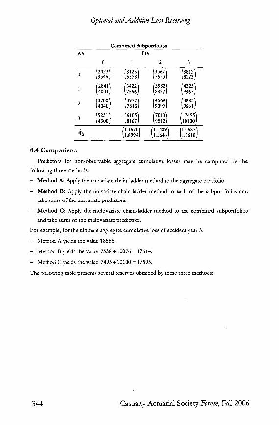
8.3 Multivariate Chain-Ladder Method

We now combine the run-off triangles of the two subportfolios into a single run-off triangle

which contains the vectors Si.k of cumulative losses:

Combined Subportfolios

AY DY

0 1 2 3

(2423 / /3123/ (3567~ 0 k3546] k6578] k7650]

/2841 / (3422] /3952] 1 ~4001] k7566] k8822]

I3700/ 13977 2 k4040] k7813]

[5231 / 3 k4300]

( 3812~ 8123]

Transforming the vectors Si,, of cumulative losses into diagonal matrices, we obtain the

following run-off triangle for the matrices Ai, k = diag(Si,,) which is completed by the

vectors ~ , of univariate chain-ladder factors:



Combined Subportfolios AY DY

0 1 2 3

0 (24203 354~)(312g 657~) 1 (28401 4000) (342~ 756~) 2 (3700 4040) (397~ 781~) 3 ('"a .0~)

/1.1738 / /1.14881 (1.0687 / ~k ~1.8950] ~1.1646] ~1.0618]

For the estimators of the variances we thus obtain

~ L 35.4968 = -14.3861

-14.3861) 5.9200

and hence

~ t =( 0.2637 0.0926 / 0.0926 0.0325]

(~CL) -1 ( 1.8616 4.5239) = 4.5239 11.1624

(~L) -1 (25876.4330 = k .73727 .6467

-73727.6467 / 210097.0596 ]

Note that estimators of the variances Y'0 and Y'3 are not needed. App134ng the multivariate chain-ladder method to the combined subportfolios )4elds the multivariate chain-ladder

predictors of the non-observable cumulative losses:



Combined Subportfolios AY DY

0 1 2 3

{2423~ /3123 / [3567~ [3812 / 0 ~3546] ~6578] ~7650] ~8123]

[2841 / /3422 / [3952 / /4223 / 1 ~4001] ~7566] ~8822] ~93671

/5231] /6105 / {7013 / [ 7495 / 3 ~4300] ~81671 ~95121 ~10100]

[1.1670 / {1.1489 / (1.0687] ~k ~1.8994] ~1.1646] ~1.0618]

8.4 Comparison Predictors for non-observable aggregate cumulative losses may be computed by the

following three methods:

- Method A: Apply the univariate chain-ladder method to the aggregate portfolio.

- Method B: Apply the univariate chain-ladder method to each of the subportfolios and

take sums of the univariate predictors.

- Method C: Apply the multivariate chain-ladder method to the combined subportfolios

and take sums of the multivariate predictors.

For example, for the ultimate aggregate cumulative loss of accident year 3,

- Method A )felds the value 18585.

- Method B yields the value 7538 + 10076 = 17614.

- Method C )fields the value 7495 + 10100 = 17595.

The following table presents several reserves obtained by these three methods:



R e s e r v e M e t h o d A M e t h o d B M e t h o d C

Accident Year 1 818 817 817



Total 12628 11655 11635

Calendar Year 4 8231 7452 7436



Total 12628 11655 11635

Due to round-off errors, some of the total reserves differ slightly from the sums of the

reserves over accident ),ears of calendar years. In the present example, the results obtained

by Methods B and C are quite similar, but they differ considerably from those obtained by

Method A.

8 . 5 P r e l i m i n a r y C o n c l u s i o n s

Of course, one should not draw general conclusions from a single numerical example.

Nevertheless, the present example and experience with other sets of data justify the

following rule of thumb:

- Method C is optimal when the model assumptions and the optimality criteria for the

multivariate chain-ladder method can be accepted.

- Method B may in many cases provide a reasonable approximation to Method C.

- Method A may be disastrous since it ignores correlation between the different lines of

business.

Experience with other sets of data also indicates that the similarities and differences between

the three methods may vary with

- the lines of business under consideration,

- the number of lines of business, and

- the number of development years.

It is therefore indispensable for the actuary to acquire practical experience for every

combined portfolio of interest.

C a s u a l t y A c t u a r i a l S o c i e t y Forum, Fa l l 2 0 0 6 3 4 5


A P P E N D I X

Here we give a p roof o f Theorem 4.5.

Proof . Consider an), q*-I-conditionally unbiased linear estimator ~ , o f ~ , . Then there

exist q , - i -measurable matrices Q.0,k-1, Q.1,,-1 . . . . . Q_,-ka-1 satisfying

n-k ~'* = E Q. ._ ,S j , ,

j=0

~--, n-k 1,% A and /..j=oM-j,k-1 j,k-I = I. Also, letting

CL .-- (~kA1 /2 Z -1A1/z ~-1 'A 1/2 Z -1A1/2 \A -1

we obtain

~CL n-k CL = y~ Q.i,k-lSs,,

j=0

~'~n-k f .~CL A and /%j=o%~j,k_l j,k-1 = I. We thus obtain

n-It ,,-~ CL \A (Q.j.,-1 - q _ j , , - . s,*-i = O.

j=0

Since

n-k -1 CL _ ( ~ , / 2 , e - , . , / , "1 (varq,-,[Sik]) - '

this yields

,.- [S . ,S , , , ] (O . . , , , _ , ) j=0 I=0

j=O

= ~.~ (Q_j,k-1 ¢"~ CL "~A [ r A1/2 *j"-IA1/2 l - " ,< . j ,k - I ] j ,k - ] | / _ . s,k-1 k s,k-I I

j=O \ s=O , .), =O.

Since i + k >_ n + 1, we also have coy 0- ' I s j , , , Si,, ] = 0 and thus

346 Casual ty Actuar ia l Society,Forum, Fall 2 0 0 6


^ eL COVq,-,E~i,k_Si,k,S;,,] = covG,-,[aCL_I~k -- Lai,/e-I'~'k~CL t.kCL, Si,k ]

^CL C O V G J , _ , E I ~ k _ , C L , s , , , ] = A i , k _ 1

^ CL n - k . = Ai,k-' X (Q_j,k-1- Q_jC',~-I ) cOVG'-I [Sj.k,Si,k] j=0

= O .

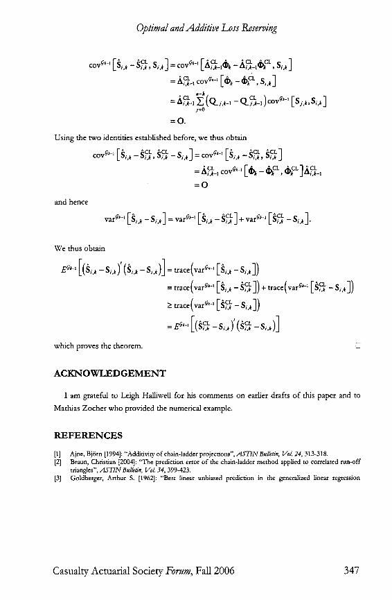
Using the two identities established before, we thus obtain

COVG,_, r ~ ~CL ~CL Si,k] COVG,_I [ g ^CL SI.k]'CL L ° / k - o i , , o , , = . . , - Si, k ,

_ . ~ C L . . . . ~ , -~ F , , ~ , ~ C L , , ~ C L " I , ~ c t . -- ~t i ,k-I ~ " L"vk -- "~"k , ~Vk ..]t'~i,k-I

= 0

and hence

^ CL -- Si,/t ] . vaV*-*ESi,'-S',']=vara*-'[S"-Si,'] + ' ° ' q * - ' F ~ : c L , -'" t : ' , , *

We thus obtain

EG*-'[(Si.,-Si,,) ' (S,.,-Si.,)]=trace(var%-'[Si.i-Si.,])

= trace(varY,_, [ ~ i , , _ ~CL ] ) + trace(vara,_l [~CL _ S i , , ] )

> t race(var %-' [S i CL -- Si, ̀ ] )

t ^ CL = 1 (S, . - S , . ) ]

which proves the theorem.

A C K N O W L E D G E M E N T

I am grateful to Leigh HalliweU for his comments on earlier drafts of this paper and to

Mathias Zocher who provided the numerical example.

R E F E R E N C E S

[1] Ajne, Bjtrn [1994]: "Additivit T of chain-ladder projections",ASTINBullain, Vol. 24, 313-318. !2] Braun, Christian [2004]: "The prediction error of the chain-ladder method applied to correlated run-off

triangles", ASTIN Bulktin, Vol. 34, 399-423. [3] Goldberger, Arthur S. [1962]: "Best linear unbiased prediction in the generalized linear regression



model",.]. American StatisticalAssocialion, Vol. 57, 369-375. [4] Hachemeister, Charles A., and James N. Stanard [1975]: "IBNR claims count estimation with static lag

functions", Unpublished. [5] Halliwell, Leigh J. [1996]: "Loss prediction by generalized least squares", PCAS, Vol. LX,'XXIII, 436-489. [6] Halliwell, Leigh J. [1997]: "Conjoint prediction of paid and incurred losses", CAS Forum Summer 1997,

V0/. I, 241-379. [7] Halliwell, Leigh J. [1999]: "Loss prediction by generalized least squares - Author's response", PC.AS, Vol.

LXXXV/, 764-769. [8] Hamer, Michael D. [1999]: "Loss prediction by generalized least squares - Discussion", PCAS, Vol.

LXXXI/ / , 748-763. [9] Hess, Klaus T., and Klaus D. Schmidt [2002]: "A comparison of models for the chain-ladder method",

Insurance Mathematics and Economics, Vol. 31, 351-364. [10] Hess, Klaus T., Klaus D. Schmidt and Mathias Zocher [2006]: "Multivariate loss reserving in the

multivariate additive model", Insurance Mathematics and Economics (in press). [11] Holmberg, Randall D. [1994]: "Correlation and the measurement of loss rese~,e variability", CAS Forum

Spring 1994, 247-278. [12] Klemmt, Heinz J. [2004]: "Trennung yon Schadenarten und Additivitiit bei Chain-Ladder Prognosen",

Paper presented at the 2004 Fall Meeting of the German ASTIN Group in Miinchen. [13] Kremer, Erhard [2005]: "The correlated chain-ladder method for reserving in case of correlated claims

developments", BIh~ter DGVFM, Vol. 27, 315-322. [14] Mack, Thomas [1993]: "Distribution-free calculation of the standard error of chain-ladder reserve

estimates", ASTIN Bulkttn, Vol. 23, 213-225. [15] Pr6hl, Carsten, and Klaus D. Schmidt [2005]: "Multivariate chain-ladder", Dresdner Schnflen zur

Versicherungsmathematik 3/2005, Paper presented at the International ASTIN Colloquium 2005 in Zfirich. [16] Quarg, Gerhard, and Thomas Mack [2004]: "Munich chain-ladder - A reserxdng method that reduces the

gap between IBNR projections based on paid losses and IBNR projections based on incurred losses", BlaSter DCVFM, Vol. 26, 597-630.

[17] Radtke, Michael, and Klaus D. Schmidt (eds.) [2004]: Handbuch gut Schadenreserderun£ Karlsruhe, Verlag Versicherungswirts cha ft.

[18] Rao, C. Radharkrischna, and Helge Toutenburg [1995]: la'near Models- Least Squares and Alternatives, Berlin - Heidelberg - New York, Springer.

[19] Schmidt, Klaus D. [1997]: "Non-optimal prediction by the chain-ladder method", Insurance, Mathematics and Economics, Vol. 21, 17-24.

[20] Schmidt, Klaus D. [1998]: "Prediction in the linear model - A direct approach", M'etr/ka, Vol. 48, 141- 147.

[21] Schmidt, Klaus D. [1999@ "Loss prediction by generalized least squares - Discussion", PCAS, Vol. LXXXV/ , 736-747.

[22] Schmidt, Klaus D. [1999b]: "Chain ladder prediction and asset liability management", Bldtter DGVM, Vol. 24, 1-9.

[23] Schmidt, Klaus D. [2004]: "Prediction", Eng,clopedia of Actuarial Sdence, Vol. 3, 1317-1321, Chichester, Wiley.

[24] Sehmidt, Klans D., and Anja Schnaus [1996]: "An extension of Mack's model for the chain-ladder method", ASTIN Bulletin, Vol. 26, 247-262.

[25] Verdier, Bertrand, and Arrur Klinger [2005]: "JAB chain - A model based calculation of paid and incurred loss development factors", Paper presented at the International ASTIN Colloquium 2005 in Ziirich.



Biography of the Author: The author is professor for actuarial mathematics at Technische Universit/it Dresden. His main interests are

mathematical models in loss reserving and reinsurance as well as linear and credibility models in non-life insurance. He has a degree in mathematics and economics from Universit/it Ziirich and a PhD in mathematics from Universit/it Mannheim. He is an academic correspondent o f the CAS and a member o f the DAV (Deutsche Aktuar-Vereinigung) with particular engagement in working parties on education and loss reserving. Besides his publications on loss reserving, the author has compiled a Bibliograpl9, on Loss Reserving which is available on the Web under ht tp: / /www.math. tu-dresden.de/s to/schmidt /ds~a'n/reserve.pdf .



C O N T E N T S

1. Introduction

2. Univariate Loss Prediction

2.1 Urfivariate Additive Model

2.2 Univariate Chain-Ladder Model

3. Estimation and Prediction in the Conditional Linear Model

3.2 Gauss-Markov Estimation

3.2 Gauss-Markov Prediction

4. M u l t i v a r i a t e Loss Prediction



5. A d d i t i v i t y



6. Estimation of the Variance Parameters



6.3 Extrapolation

6.4 Iteration

6.5 External Information

7. Remarks

8. A N u m e r i c a l E x a m p l e

8.1 The Data

8.2 Univariate Chain-Ladder Method

8.3 Multivariate Chain-Ladder Method

8.4 Comparison

350 C a s u a l t y A c t u a r i a l S o c i e t y Forum, Fal l 2006


8.5 Preliminary Conclusions

Appendix

Acknowledgement

References


Documents

Optimal and Additive Loss Reserving for Dependent Lines of

References

Casualty Actuarial Society Forum, Fall 2006 351