Claims Reserving With R

Claims reserving with R:

ChainLadder-0.2.0 Package Vignette

Alessandro Carrato, Markus Gesmann, Dan Murphy,

Mario Wuthrich and Wayne Zhang

March 4, 2015

Abstract

The ChainLadder package provides various statistical methods which are

typically used for the estimation of outstanding claims reserves in general

insurance, including those to estimate the claims development results as re-

quired under Solvency II.

1

Contents

1 Introduction 4

1.1 Claims reserving in insurance . . . . . . . . . . . . . . . . . . . . . 4

2 The ChainLadder package 5

2.1 Motivation . . . . . . . . . . . . . . . . . . . . . . . . . . . . . . . 5

2.2 Brief package overview . . . . . . . . . . . . . . . . . . . . . . . . 5

2.3 Installation . . . . . . . . . . . . . . . . . . . . . . . . . . . . . . . 6

3 Using the ChainLadder package 6

3.1 Working with triangles . . . . . . . . . . . . . . . . . . . . . . . . 6

3.1.1 Plotting triangles . . . . . . . . . . . . . . . . . . . . . . . 8

3.1.2 Transforming triangles between cumulative and incrementalrepresentation . . . . . . . . . . . . . . . . . . . . . . . . . 9

3.1.3 Importing triangles from external data sources . . . . . . . . 10

3.1.4 Copying and pasting from MS Excel . . . . . . . . . . . . . 13

4 Chain-ladder methods 13

4.1 Basic idea . . . . . . . . . . . . . . . . . . . . . . . . . . . . . . . 13

4.2 Mack chain-ladder . . . . . . . . . . . . . . . . . . . . . . . . . . . 17

4.3 Munich chain-ladder . . . . . . . . . . . . . . . . . . . . . . . . . . 21

4.4 Bootstrap chain-ladder . . . . . . . . . . . . . . . . . . . . . . . . 23

4.5 Multivariate chain-ladder . . . . . . . . . . . . . . . . . . . . . . . 26

4.6 The "triangles" class . . . . . . . . . . . . . . . . . . . . . . . . 27

4.7 Separate chain ladder ignoring correlations . . . . . . . . . . . . . . 28

4.8 Multivariate chain ladder using seemingly unrelated regressions . . . 30

4.9 Other residual covariance estimation methods . . . . . . . . . . . . 31

4.10 Model with intercepts . . . . . . . . . . . . . . . . . . . . . . . . . 34

4.11 Joint modelling of the paid and incurred losses . . . . . . . . . . . . 36

5 Clark’s methods 37

5.1 Clark’s LDF method . . . . . . . . . . . . . . . . . . . . . . . . . . 38

5.2 Clark’s Cap Cod method . . . . . . . . . . . . . . . . . . . . . . . 40

2

6 Generalised linear model methods 41

7 One year claims development result 46

7.1 CDR functions . . . . . . . . . . . . . . . . . . . . . . . . . . . . . 46

8 Model Validation with tweedieReserve 47

9 Using ChainLadder with RExcel and SWord 49

10 Further resources 50

10.1 Other insurance related R packages . . . . . . . . . . . . . . . . . . 50

10.2 Presentations . . . . . . . . . . . . . . . . . . . . . . . . . . . . . 51

10.3 Further reading . . . . . . . . . . . . . . . . . . . . . . . . . . . . 51

11 Training and consultancy 51

References 55

3

1 Introduction

1.1 Claims reserving in insurance

The insurance industry, unlike other industries, does not sell products as such butpromises. An insurance policy is a promise by the insurer to the policyholder to payfor future claims for an upfront received premium.

As a result insurers don’t know the upfront cost for their service, but rely on histor-ical data analysis and judgement to predict a sustainable price for their offering. InGeneral Insurance (or Non-Life Insurance, e.g. motor, property and casualty insur-ance) most policies run for a period of 12 months. However, the claims paymentprocess can take years or even decades. Therefore often not even the delivery dateof their product is known to insurers.

In particular losses arising from casualty insurance can take a long time to settle andeven when the claims are acknowledged it may take time to establish the extentof the claims settlement cost. Claims can take years to materialize. A complexand costly example are the claims from asbestos liabilities, particularly those inconnection with mesothelioma and lung damage arising from prolonged exposureto asbestos. A research report by a working party of the Institute and Faculty ofActuaries estimated that the un-discounted cost of UK mesothelioma-related claimsto the UK Insurance Market for the period 2009 to 2050 could be around £10bn,see [GBB+09]. The cost for asbestos related claims in the US for the worldwideinsurance industry was estimate to be around $120bn in 2002, see [Mic02].

Thus, it should come as no surprise that the biggest item on the liabilities side of aninsurer’s balance sheet is often the provision or reserves for future claims payments.Those reserves can be broken down in case reserves (or outstanding claims), whichare losses already reported to the insurance company and losses that are incurredbut not reported (IBNR) yet.

Historically, reserving was based on deterministic calculations with pen and paper,combined with expert judgement. Since the 1980’s, with the arrival of personalcomputer, spreadsheet software became very popular for reserving. Spreadsheets notonly reduced the calculation time, but allowed actuaries to test different scenariosand the sensitivity of their forecasts.

As the computer became more powerful, ideas of more sophisticated models startedto evolve. Changes in regulatory requirements, e.g. Solvency II1 in Europe, havefostered further research and promoted the use of stochastic and statistical tech-niques. In particular, for many countries extreme percentiles of reserve deteriorationover a fixed time period have to be estimated for the purpose of capital setting.

Over the years several methods and models have been developed to estimate boththe level and variability of reserves for insurance claims, see [Sch11] or [PR02] foran overview.

1See http://ec.europa.eu/internal_market/insurance/solvency/index_en.htm

4

http://ec.europa.eu/internal_market/insurance/solvency/index_en.htm

In practice the Mack chain-ladder and bootstrap chain-ladder models are used bymany actuaries along with stress testing / scenario analysis and expert judgementto estimate ranges of reasonable outcomes, see the surveys of UK actuaries in2002, [LFK+02], and across the Lloyd’s market in 2012, [Orr12].

2 The ChainLadder package

2.1 Motivation

The ChainLadder [GMZ14] package provides various statistical methods which aretypically used for the estimation of outstanding claims reserves in general insurance.The package started out of presentations given by Markus Gesmann at the Stochas-tic Reserving Seminar at the Institute of Actuaries in 2007 and 2008, followed bytalks at Casualty Actuarial Society (CAS) meetings joined by Dan Murphy in 2008and Wayne Zhang in 2010.

Implementing reserving methods in R has several advantages. R provides:

• a rich language for statistical modelling and data manipulations allowing fastprototyping

• a very active user base, which publishes many extension

• many interfaces to data bases and other applications, such as MS Excel

• an established framework for End User Computing, including documentation,testing and workflows with version control systems

• code written in plain text files, allowing effective knowledge transfer

• an effective way to collaborate over the internet

• built in functions to create reproducible research reports2

• in combination with other tools such as LATEX and Sweave or Markdown easyto set up automated reporting facilities

• access to academic research, which is often first implemented in R

2.2 Brief package overview

This vignette will give the reader a brief overview of the functionality of the Chain-Ladder package. The functions are discussed and explained in more detail in therespective help files and examples, see also [Ges14].

A set of demos is shipped with the packages and the list of demos is available via:

2For an example see the project: Formatted Actuarial Vignettes in R, http://www.favir.net/

5

http://www.favir.net/

R> demo(package="ChainLadder")

and can be executed via

R> library(ChainLadder)

R> demo("demo name")

For more information and examples see the project web site: http://code.google.com/p/chainladder/

2.3 Installation

You can install ChainLadder in the usual way from CRAN, e.g.:

R> install.packages('ChainLadder')

For more details about installing packages see [Tea12b]. The installation was suc-cessful if the command library(ChainLadder) gives you the following message:

R> library(ChainLadder)

ChainLadder version 0.2.0

Type ?ChainLadder to access overall documentation and

vignette('ChainLadder') for the package vignette.

Type demo(ChainLadder) to get an idea of the functionality of this package.

See demo(package='ChainLadder') for a list of more demos.

More information is available on the ChainLadder project web-site:

http://code.google.com/p/chainladder/

To suppress this message use the statement:

suppressPackageStartupMessages(library(ChainLadder))

3 Using the ChainLadder package

3.1 Working with triangles

Historical insurance data is often presented in form of a triangle structure, showingthe development of claims over time for each exposure (origin) period. An originperiod could be the year the policy was written or earned, or the loss occurrence

6



period. Of course the origin period doesn’t have to be yearly, e.g. quarterly ormonthly origin periods are also often used. The development period of an originperiod is also called age or lag. Data on the diagonals present payments in thesame calendar period. Note, data of individual policies is usually aggregated tohomogeneous lines of business, division levels or perils.

Most reserving methods of the ChainLadder package expect triangles as input datasets with development periods along the columns and the origin period in rows. Thepackage comes with several example triangles. The following R command will listthem all:

R> require(ChainLadder)

R> data(package="ChainLadder")

Let’s look at one example triangle more closely. The following triangle shows datafrom the Reinsurance Association of America (RAA):

R> ## Sample triangle

R> RAA

dev

origin 1 2 3 4 5 6 7 8 9 10

1981 5012 8269 10907 11805 13539 16181 18009 18608 18662 18834

1982 106 4285 5396 10666 13782 15599 15496 16169 16704 NA

1983 3410 8992 13873 16141 18735 22214 22863 23466 NA NA

1984 5655 11555 15766 21266 23425 26083 27067 NA NA NA

1985 1092 9565 15836 22169 25955 26180 NA NA NA NA

1986 1513 6445 11702 12935 15852 NA NA NA NA NA

1987 557 4020 10946 12314 NA NA NA NA NA NA

1988 1351 6947 13112 NA NA NA NA NA NA NA

1989 3133 5395 NA NA NA NA NA NA NA NA

1990 2063 NA NA NA NA NA NA NA NA NA

This triangle shows the known values of loss from each origin year and of annualevaluations thereafter. For example, the known values of loss originating from the1988 exposure period are 1351, 6947, and 13112 as of year ends 1988, 1989, and1990, respectively. The latest diagonal – i.e., the vector 18834, 16704, . . . 2063from the upper right to the lower left – shows the most recent evaluation available.The column headings – 1, 2,. . . , 10 – hold the ages (in years) of the observationsin the column relative to the beginning of the exposure period. For example, forthe 1988 origin year, the age of the 1351 value, evaluated as of 1988-12-31, is threeyears.

The objective of a reserving exercise is to forecast the future claims development inthe bottom right corner of the triangle and potential further developments beyonddevelopment age 10. Eventually all claims for a given origin period will be settled,

7

but it is not always obvious to judge how many years or even decades it will take.We speak of long and short tail business depending on the time it takes to pay allclaims.

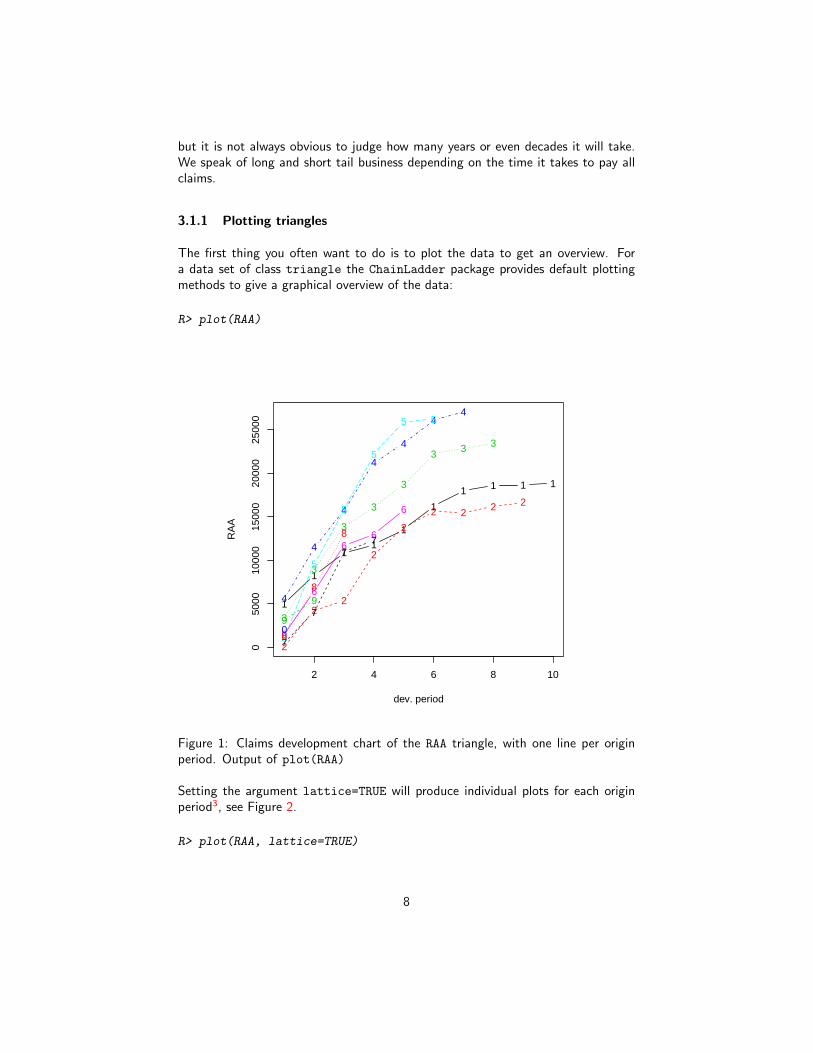
3.1.1 Plotting triangles

The first thing you often want to do is to plot the data to get an overview. Fora data set of class triangle the ChainLadder package provides default plottingmethods to give a graphical overview of the data:

R> plot(RAA)

1

1

11

1

1

1 1 1 1

2 4 6 8 10

050

0010

000

1500

020

000

2500

0

dev. period

RA

A

2

22

2

2

2 2 2 2

3

3

3

3

3

3 3 3

4

4

4

4

4

44

5

5

5

5

5 5

6

6

66

6

7

7

77

8

8

8

9

9

0

Figure 1: Claims development chart of the RAA triangle, with one line per originperiod. Output of plot(RAA)

Setting the argument lattice=TRUE will produce individual plots for each originperiod3, see Figure 2.

R> plot(RAA, lattice=TRUE)

8

dev. period

0

5000

10000

15000

20000

25000

●

●

● ●●

●● ● ● ●

1981

2 4 6 8 10

●

●●

●

●● ● ● ●

1982

●

●

●●

●

● ● ●

1983

2 4 6 8 10

●

●

●

●●

● ●

1984

●

●

●

●

● ●

1985

●

●

●●

●

1986

●

●

●●

1987

0

5000

10000

15000

20000

25000

●

●

●

1988

0

5000

10000

15000

20000

25000

2 4 6 8 10

●●

1989

●

1990

Figure 2: Claims development chart of the RAA triangle, with individual panels foreach origin period. Output of plot(RAA, lattice=TRUE)

You will notice from the plots in Figures 1 and 2 that the triangle RAA presentsclaims developments for the origin years 1981 to 1990 in a cumulative form. For moreinformation on the triangle plotting functions see the help pages of plot.triangle,e.g. via

R> ?plot.triangle

3.1.2 Transforming triangles between cumulative and incremental repre-

sentation

The ChainLadder packages comes with two helper functions, cum2incr and incr2cumto transform cumulative triangles into incremental triangles and vice versa:

R> raa.inc <- cum2incr(RAA)

R> ## Show first origin period and its incremental development

3ChainLadder uses the lattice package for plotting the development of the origin years inseparate panels.

9

http://cran.r-project.org/package=lattice

R> raa.inc[1,]

1 2 3 4 5 6 7 8 9 10

5012 3257 2638 898 1734 2642 1828 599 54 172

R> raa.cum <- incr2cum(raa.inc)

R> ## Show first origin period and its cumulative development

R> raa.cum[1,]

1 2 3 4 5 6 7 8 9 10

5012 8269 10907 11805 13539 16181 18009 18608 18662 18834

3.1.3 Importing triangles from external data sources

In most cases you want to analyse your own data, usually stored in data bases. Rmakes it easy to access data using SQL statements, e.g. via an ODBC connection4,for more details see [Tea12a]. The ChainLadder packages includes a demo toshowcase how data can be imported from a MS Access data base, see:

R> demo(DatabaseExamples)

In this section we use data stored in a CSV-file5 to demonstrate some typical op-erations you will want to carry out with data stored in data bases. CSV standsfor comma separated values, stored in a text file. Note many European countriesuse a comma as decimal point and a semicolon as field separator, see also the helpfile to read.csv2. In most cases your triangles will be stored in tables and notin a classical triangle shape. The ChainLadder package contains a CSV-file withsample data in a long table format. We read the data into R’s memory with theread.csv command and look at the first couple of rows and summarise it:

R> filename <- file.path(system.file("Database",

package="ChainLadder"),

"TestData.csv")

R> myData <- read.csv(filename)

R> head(myData)

origin dev value lob

1 1977 1 153638 ABC

2 1978 1 178536 ABC

3 1979 1 210172 ABC

4See the RODBC and DBI packages5Please ensure that your CSV-file is free from formatting, e.g. characters to separate units of

thousands, as those columns will be read as characters or factors rather than numerical values.

10

http://cran.r-project.org/package=RODBC

http://cran.r-project.org/package=DBI

4 1980 1 211448 ABC

5 1981 1 219810 ABC

6 1982 1 205654 ABC

R> summary(myData)


Min. : 1 Min. : 1.00 Min. : -17657 AutoLiab :105

1st Qu.: 3 1st Qu.: 2.00 1st Qu.: 10324 GeneralLiab :105

Median : 6 Median : 4.00 Median : 72468 M3IR5 :105

Mean : 642 Mean : 4.61 Mean : 176632 ABC : 66

3rd Qu.:1979 3rd Qu.: 7.00 3rd Qu.: 197716 CommercialAutoPaid: 55

Max. :1991 Max. :14.00 Max. :3258646 GenIns : 55

(Other) :210

Let’s focus on one subset of the data. We select the RAA data again:

R> raa <- subset(myData, lob %in% "RAA")

R> head(raa)


67 1981 1 5012 RAA

68 1982 1 106 RAA

69 1983 1 3410 RAA

70 1984 1 5655 RAA

71 1985 1 1092 RAA

72 1986 1 1513 RAA

To transform the long table of the RAA data into a triangle we use the functionas.triangle. The arguments we have to specify are the column names of theorigin and development period and further the column which contains the values:

R> raa.tri <- as.triangle(raa,

origin="origin",

dev="dev",

value="value")

R> raa.tri

dev

origin 1 2 3 4 5 6 7 8 9 10

1981 5012 3257 2638 898 1734 2642 1828 599 54 172

1982 106 4179 1111 5270 3116 1817 -103 673 535 NA

1983 3410 5582 4881 2268 2594 3479 649 603 NA NA

1984 5655 5900 4211 5500 2159 2658 984 NA NA NA

11

1985 1092 8473 6271 6333 3786 225 NA NA NA NA

1986 1513 4932 5257 1233 2917 NA NA NA NA NA

1987 557 3463 6926 1368 NA NA NA NA NA NA

1988 1351 5596 6165 NA NA NA NA NA NA NA

1989 3133 2262 NA NA NA NA NA NA NA NA

1990 2063 NA NA NA NA NA NA NA NA NA

We note that the data has been stored as an incremental data set. As mentionedabove, we could now use the function incr2cum to transform the triangle into acumulative format.

We can transform a triangle back into a data frame structure:

R> raa.df <- as.data.frame(raa.tri, na.rm=TRUE)

R> head(raa.df)

origin dev value

1981-1 1981 1 5012

1982-1 1982 1 106

1983-1 1983 1 3410

1984-1 1984 1 5655

1985-1 1985 1 1092

1986-1 1986 1 1513

This is particularly helpful when you would like to store your results back into adata base. Figure 3 gives you an idea of a potential data flow between R and databases.

RODBCsqlQuery

as.triangle

R: ChainLadder

sqlSave

DB

stored

ract

rm les

many

ck into

Figure 3: Flow chart of data between R and data bases.

12

3.1.4 Copying and pasting from MS Excel

Small data sets in Excel can be transfered to R backwards and forwards with viathe clipboard under MS Windows.

Copying from Excel to R Select a data set in Excel and copy it into the clipboard,then go to R and type:

R> x <- read.table(file="clipboard", sep="\t", na.strings="")

Copying from R to Excel Suppose you would like to copy the RAA triangle intoExcel, then the following statement would copy the data into the clipboard:

R> write.table(RAA, file="clipboard", sep="\t", na="")

Now you can paste the content into Excel. Please note that you can’t copy listsstructures from R to Excel easily.

4 Chain-ladder methods

The classical chain-ladder is a deterministic algorithm to forecast claims based onhistorical data. It assumes that the proportional developments of claims from onedevelopment period to the next are the same for all origin years.

4.1 Basic idea

Most commonly as a first step, the age-to-age link ratios are calculated as the volumeweighted average development ratios of a cumulative loss development triangle fromone development period to the next Cik, i, k = 1, . . . , n.

fk =

∑n−ki=1 Ci,k+1∑n−ki=1 Ci,k

(1)

R> n <- 10

R> f <- sapply(1:(n-1),

function(i){

sum(RAA[c(1:(n-i)),i+1])/sum(RAA[c(1:(n-i)),i])

}

)

R> f

[1] 2.999 1.624 1.271 1.172 1.113 1.042 1.033 1.017 1.009

13

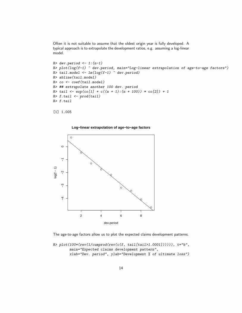
Often it is not suitable to assume that the oldest origin year is fully developed. Atypical approach is to extrapolate the development ratios, e.g. assuming a log-linearmodel.

R> dev.period <- 1:(n-1)

R> plot(log(f-1) ~ dev.period, main="Log-linear extrapolation of age-to-age factors")

R> tail.model <- lm(log(f-1) ~ dev.period)

R> abline(tail.model)

R> co <- coef(tail.model)

R> ## extrapolate another 100 dev. period

R> tail <- exp(co[1] + c((n + 1):(n + 100)) * co[2]) + 1

R> f.tail <- prod(tail)

R> f.tail

[1] 1.005

●

●

●

●

●

●

●

●

●

2 4 6 8

−4

−3

−2

−1

0

Log−linear extrapolation of age−to−age factors

dev.period

log(

f − 1

)

The age-to-age factors allow us to plot the expected claims development patterns.

R> plot(100*(rev(1/cumprod(rev(c(f, tail[tail>1.0001]))))), t="b",

main="Expected claims development pattern",

xlab="Dev. period", ylab="Development % of ultimate loss")

14

●

●

●

●

●

●

●

●● ● ● ● ● ●

2 4 6 8 10 12 14

2040

6080

100

Expected claims development pattern

Dev. period

Dev

elop

men

t % o

f ulti

mat

e lo

ss

The link ratios are then applied to the latest known cumulative claims amount toforecast the next development period. The squaring of the RAA triangle is calcu-lated below, where an ultimate column is appended to the right to accommodatethe expected development beyond the oldest age (10) of the triangle due to the tailfactor (1.005) being greater than unity.

R> f <- c(f, f.tail)

R> fullRAA <- cbind(RAA, Ult = rep(0, 10))

R> for(k in 1:n){

fullRAA[(n-k+1):n, k+1] <- fullRAA[(n-k+1):n,k]*f[k]

}

R> round(fullRAA)

1 2 3 4 5 6 7 8 9 10 Ult

1981 5012 8269 10907 11805 13539 16181 18009 18608 18662 18834 18928

1982 106 4285 5396 10666 13782 15599 15496 16169 16704 16858 16942

1983 3410 8992 13873 16141 18735 22214 22863 23466 23863 24083 24204

1984 5655 11555 15766 21266 23425 26083 27067 27967 28441 28703 28847

1985 1092 9565 15836 22169 25955 26180 27278 28185 28663 28927 29072

1986 1513 6445 11702 12935 15852 17649 18389 19001 19323 19501 19599

1987 557 4020 10946 12314 14428 16064 16738 17294 17587 17749 17838

1988 1351 6947 13112 16664 19525 21738 22650 23403 23800 24019 24139

15

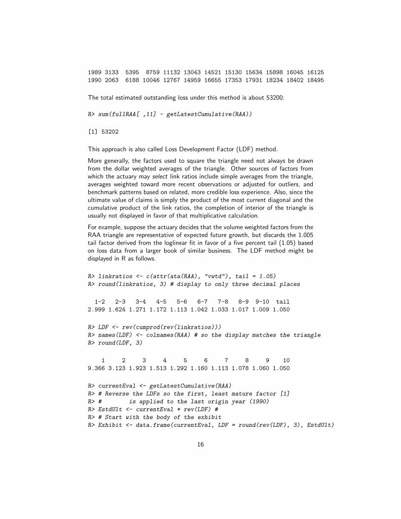
1989 3133 5395 8759 11132 13043 14521 15130 15634 15898 16045 16125

1990 2063 6188 10046 12767 14959 16655 17353 17931 18234 18402 18495

The total estimated outstanding loss under this method is about 53200:

R> sum(fullRAA[ ,11] - getLatestCumulative(RAA))

[1] 53202

This approach is also called Loss Development Factor (LDF) method.

More generally, the factors used to square the triangle need not always be drawnfrom the dollar weighted averages of the triangle. Other sources of factors fromwhich the actuary may select link ratios include simple averages from the triangle,averages weighted toward more recent observations or adjusted for outliers, andbenchmark patterns based on related, more credible loss experience. Also, since theultimate value of claims is simply the product of the most current diagonal and thecumulative product of the link ratios, the completion of interior of the triangle isusually not displayed in favor of that multiplicative calculation.

For example, suppose the actuary decides that the volume weighted factors from theRAA triangle are representative of expected future growth, but discards the 1.005tail factor derived from the loglinear fit in favor of a five percent tail (1.05) basedon loss data from a larger book of similar business. The LDF method might bedisplayed in R as follows.

R> linkratios <- c(attr(ata(RAA), "vwtd"), tail = 1.05)

R> round(linkratios, 3) # display to only three decimal places

1-2 2-3 3-4 4-5 5-6 6-7 7-8 8-9 9-10 tail

2.999 1.624 1.271 1.172 1.113 1.042 1.033 1.017 1.009 1.050

R> LDF <- rev(cumprod(rev(linkratios)))

R> names(LDF) <- colnames(RAA) # so the display matches the triangle

R> round(LDF, 3)

1 2 3 4 5 6 7 8 9 10

9.366 3.123 1.923 1.513 1.292 1.160 1.113 1.078 1.060 1.050

R> currentEval <- getLatestCumulative(RAA)

R> # Reverse the LDFs so the first, least mature factor [1]

R> # is applied to the last origin year (1990)

R> EstdUlt <- currentEval * rev(LDF) #

R> # Start with the body of the exhibit

R> Exhibit <- data.frame(currentEval, LDF = round(rev(LDF), 3), EstdUlt)

16

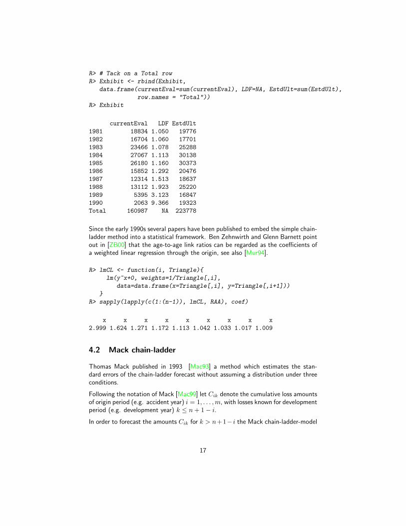
R> # Tack on a Total row

R> Exhibit <- rbind(Exhibit,

data.frame(currentEval=sum(currentEval), LDF=NA, EstdUlt=sum(EstdUlt),

row.names = "Total"))

R> Exhibit

currentEval LDF EstdUlt

1981 18834 1.050 19776

1982 16704 1.060 17701

1983 23466 1.078 25288

1984 27067 1.113 30138

1985 26180 1.160 30373

1986 15852 1.292 20476

1987 12314 1.513 18637

1988 13112 1.923 25220

1989 5395 3.123 16847

1990 2063 9.366 19323

Total 160987 NA 223778

Since the early 1990s several papers have been published to embed the simple chain-ladder method into a statistical framework. Ben Zehnwirth and Glenn Barnett pointout in [ZB00] that the age-to-age link ratios can be regarded as the coefficients ofa weighted linear regression through the origin, see also [Mur94].

R> lmCL <- function(i, Triangle){

lm(y~x+0, weights=1/Triangle[,i],

data=data.frame(x=Triangle[,i], y=Triangle[,i+1]))

}

R> sapply(lapply(c(1:(n-1)), lmCL, RAA), coef)

x x x x x x x x x

2.999 1.624 1.271 1.172 1.113 1.042 1.033 1.017 1.009

4.2 Mack chain-ladder

Thomas Mack published in 1993 [Mac93] a method which estimates the stan-dard errors of the chain-ladder forecast without assuming a distribution under threeconditions.

Following the notation of Mack [Mac99] let Cik denote the cumulative loss amountsof origin period (e.g. accident year) i = 1, . . . ,m, with losses known for developmentperiod (e.g. development year) k ≤ n+ 1− i.

In order to forecast the amounts Cik for k > n+1− i the Mack chain-ladder-model

17

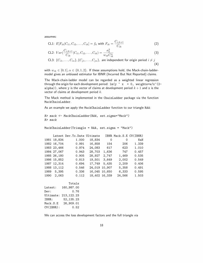
assumes:

CL1: E[Fik|Ci1, Ci2, . . . , Cik] = fk with Fik =Ci,k+1

Cik(2)

CL2: V ar(Ci,k+1

Cik|Ci1, Ci2, . . . , Cik) =

σ2k

wikCαik

(3)

CL3: {Ci1, . . . , Cin}, {Cj1, . . . , Cjn}, are independent for origin period i 6= j

(4)

with wik ∈ [0; 1], α ∈ {0, 1, 2}. If these assumptions hold, the Mack-chain-ladder-model gives an unbiased estimator for IBNR (Incurred But Not Reported) claims.

The Mack-chain-ladder model can be regarded as a weighted linear regressionthrough the origin for each development period: lm(y ~ x + 0, weights=w/x^(2-

alpha)), where y is the vector of claims at development period k + 1 and x is thevector of claims at development period k.

The Mack method is implemented in the ChainLadder package via the functionMackChainLadder.

As an example we apply the MackChainLadder function to our triangle RAA:

R> mack <- MackChainLadder(RAA, est.sigma="Mack")

R> mack

MackChainLadder(Triangle = RAA, est.sigma = "Mack")

Latest Dev.To.Date Ultimate IBNR Mack.S.E CV(IBNR)

1981 18,834 1.000 18,834 0 0 NaN

1982 16,704 0.991 16,858 154 206 1.339

1983 23,466 0.974 24,083 617 623 1.010

1984 27,067 0.943 28,703 1,636 747 0.457

1985 26,180 0.905 28,927 2,747 1,469 0.535

1986 15,852 0.813 19,501 3,649 2,002 0.549

1987 12,314 0.694 17,749 5,435 2,209 0.406

1988 13,112 0.546 24,019 10,907 5,358 0.491

1989 5,395 0.336 16,045 10,650 6,333 0.595

1990 2,063 0.112 18,402 16,339 24,566 1.503

Totals

Latest: 160,987.00

Dev: 0.76

Ultimate: 213,122.23

IBNR: 52,135.23

Mack.S.E 26,909.01

CV(IBNR): 0.52

We can access the loss development factors and the full triangle via

18

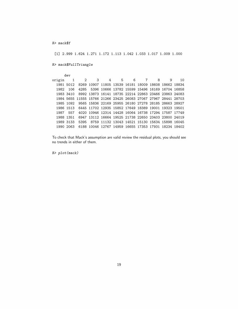
R> mack$f

[1] 2.999 1.624 1.271 1.172 1.113 1.042 1.033 1.017 1.009 1.000

R> mack$FullTriangle

dev

origin 1 2 3 4 5 6 7 8 9 10

1981 5012 8269 10907 11805 13539 16181 18009 18608 18662 18834

1982 106 4285 5396 10666 13782 15599 15496 16169 16704 16858

1983 3410 8992 13873 16141 18735 22214 22863 23466 23863 24083

1984 5655 11555 15766 21266 23425 26083 27067 27967 28441 28703

1985 1092 9565 15836 22169 25955 26180 27278 28185 28663 28927

1986 1513 6445 11702 12935 15852 17649 18389 19001 19323 19501

1987 557 4020 10946 12314 14428 16064 16738 17294 17587 17749

1988 1351 6947 13112 16664 19525 21738 22650 23403 23800 24019

1989 3133 5395 8759 11132 13043 14521 15130 15634 15898 16045

1990 2063 6188 10046 12767 14959 16655 17353 17931 18234 18402

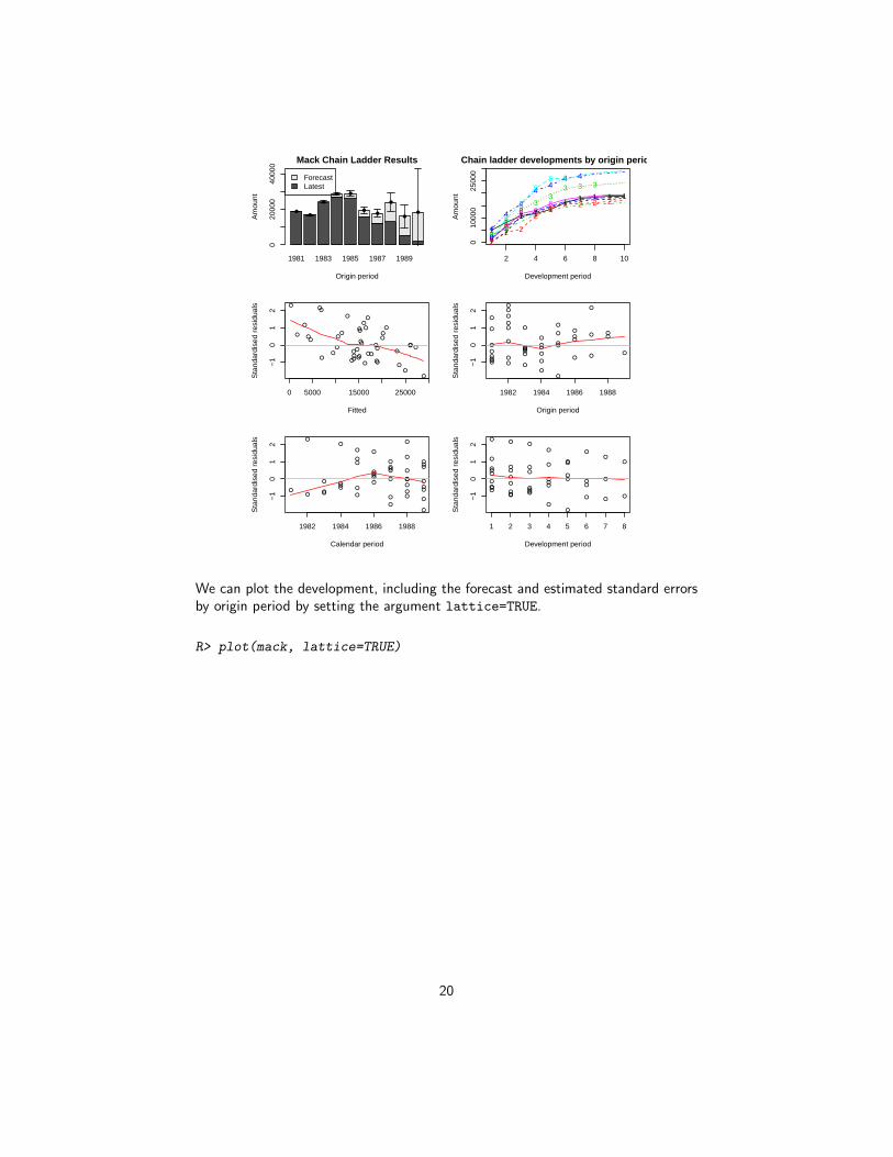
To check that Mack’s assumption are valid review the residual plots, you should seeno trends in either of them.

R> plot(mack)

19

1981 1983 1985 1987 1989

ForecastLatest

Mack Chain Ladder Results

Origin period

Am

ount

020

000

4000

0

●●

●

● ●

●●

●

●●

2 4 6 8 10

010

000

2500

0

Chain ladder developments by origin period

Development period

Am

ount

11

1 1 11

1 1 1 1

22 2

22

2 2 2 2

3

3

33

33 3 3

4

44

44

4 4

5

5

5

55 5

6

6

6 66

77

7 7

8

8

8

99

0

●

●

●

●

●

●● ●

●

●●

●

●

●

●

●

●

●

●

●

●●

●●●

●

●

●

●

●●

●

●

●

●

●

●

●●

●

●

●●

●

0 5000 15000 25000

−1

01

2

Fitted

Sta

ndar

dise

d re

sidu

als

●

●

●

●

●

●● ●

●

●●

●

●

●

●

●

●

●

●

●

●●

● ●●

●

●

●

●

●●

●

●

●

●

●

●

●●

●

●

●●

●

1982 1984 1986 1988

−1

01

2

Origin period

Sta

ndar

dise

d re

sidu

als

●

●

●

●

●

●● ●

●

●●

●

●

●

●

●

●

●

●

●

●●

● ●●

●

●

●

●

●●

●

●

●

●

●

●

●●

●

●

●●

●

1982 1984 1986 1988

−1

01

2

Calendar period

Sta

ndar

dise

d re

sidu

als

●

●

●

●

●

●●●

●

●●

●

●

●

●

●

●

●

●

●

●●

●●●

●

●

●

●

● ●

●

●

●

●

●

●

●●

●

●

●●

●

1 2 3 4 5 6 7 8

−1

01

2

Development period

Sta

ndar

dise

d re

sidu

als

We can plot the development, including the forecast and estimated standard errorsby origin period by setting the argument lattice=TRUE.

R> plot(mack, lattice=TRUE)

20

Chain ladder developments by origin period

Development period

Am

ount

0

10000

20000

30000

40000

1981

2 4 6 8 10

1982 1983

2 4 6 8 10

1984

1985 1986 1987

0

10000

20000

30000

40000

1988

0

10000

20000

30000

40000

2 4 6 8 10

1989 1990

Chain ladder dev. Mack's S.E.

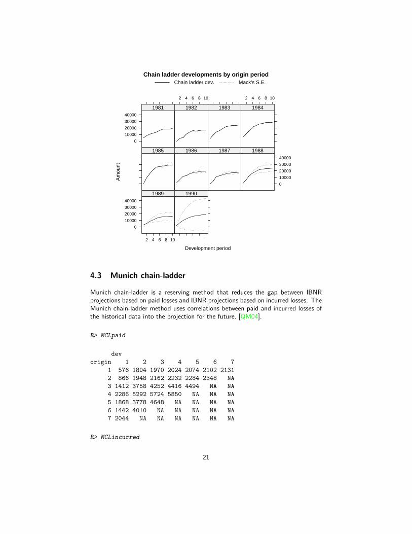
4.3 Munich chain-ladder

Munich chain-ladder is a reserving method that reduces the gap between IBNRprojections based on paid losses and IBNR projections based on incurred losses. TheMunich chain-ladder method uses correlations between paid and incurred losses ofthe historical data into the projection for the future. [QM04].

R> MCLpaid

dev

origin 1 2 3 4 5 6 7

1 576 1804 1970 2024 2074 2102 2131

2 866 1948 2162 2232 2284 2348 NA

3 1412 3758 4252 4416 4494 NA NA

4 2286 5292 5724 5850 NA NA NA

5 1868 3778 4648 NA NA NA NA

6 1442 4010 NA NA NA NA NA

7 2044 NA NA NA NA NA NA

R> MCLincurred

21

dev

origin 1 2 3 4 5 6 7

1 978 2104 2134 2144 2174 2182 2174

2 1844 2552 2466 2480 2508 2454 NA

3 2904 4354 4698 4600 4644 NA NA

4 3502 5958 6070 6142 NA NA NA

5 2812 4882 4852 NA NA NA NA

6 2642 4406 NA NA NA NA NA

7 5022 NA NA NA NA NA NA

R> op <- par(mfrow=c(1,2))

R> plot(MCLpaid)

R> plot(MCLincurred)

R> par(op)

R> # Following the example in Quarg's (2004) paper:

R> MCL <- MunichChainLadder(MCLpaid, MCLincurred, est.sigmaP=0.1, est.sigmaI=0.1)

R> MCL

MunichChainLadder(Paid = MCLpaid, Incurred = MCLincurred, est.sigmaP = 0.1,

est.sigmaI = 0.1)

Latest Paid Latest Incurred Latest P/I Ratio Ult. Paid Ult. Incurred

1 2,131 2,174 0.980 2,131 2,174

2 2,348 2,454 0.957 2,383 2,444

3 4,494 4,644 0.968 4,597 4,629

4 5,850 6,142 0.952 6,119 6,176

5 4,648 4,852 0.958 4,937 4,950

6 4,010 4,406 0.910 4,656 4,665

7 2,044 5,022 0.407 7,549 7,650

Ult. P/I Ratio

1 0.980

2 0.975

3 0.993

4 0.991

5 0.997

6 0.998

7 0.987

Totals

Paid Incurred P/I Ratio

Latest: 25,525 29,694 0.86

Ultimate: 32,371 32,688 0.99

R> plot(MCL)

22

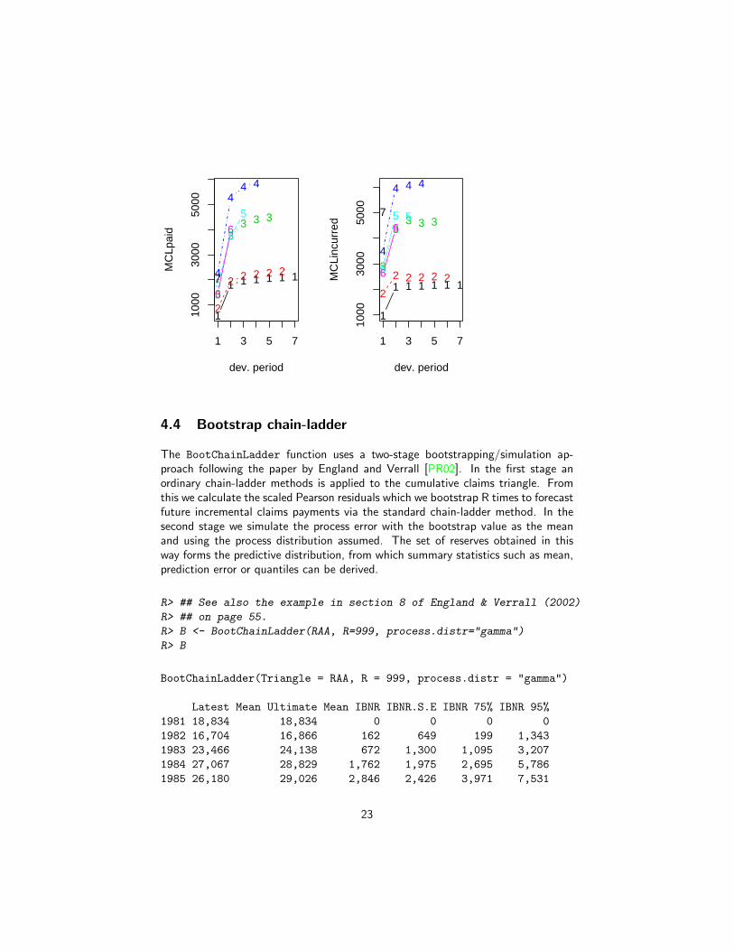
1

1 1 1 1 1 1

1 3 5 7

1000

3000

5000

dev. period

MC

Lpai

d

2

2 2 2 2 2

3

33 3 3

4

44 4

5

5

5

6

6

7

1

1 1 1 1 1 1

1 3 5 7

1000

3000

5000

dev. period

MC

Linc

urre

d

2

2 2 2 2 23

33 3 3

4

4 4 4

5

5 5

6

67

4.4 Bootstrap chain-ladder

The BootChainLadder function uses a two-stage bootstrapping/simulation ap-proach following the paper by England and Verrall [PR02]. In the first stage anordinary chain-ladder methods is applied to the cumulative claims triangle. Fromthis we calculate the scaled Pearson residuals which we bootstrap R times to forecastfuture incremental claims payments via the standard chain-ladder method. In thesecond stage we simulate the process error with the bootstrap value as the meanand using the process distribution assumed. The set of reserves obtained in thisway forms the predictive distribution, from which summary statistics such as mean,prediction error or quantiles can be derived.

R> ## See also the example in section 8 of England & Verrall (2002)

R> ## on page 55.

R> B <- BootChainLadder(RAA, R=999, process.distr="gamma")

R> B

BootChainLadder(Triangle = RAA, R = 999, process.distr = "gamma")

Latest Mean Ultimate Mean IBNR IBNR.S.E IBNR 75% IBNR 95%

1981 18,834 18,834 0 0 0 0

1982 16,704 16,866 162 649 199 1,343

1983 23,466 24,138 672 1,300 1,095 3,207

1984 27,067 28,829 1,762 1,975 2,695 5,786

1985 26,180 29,026 2,846 2,426 3,971 7,531

23

1986 15,852 19,614 3,762 2,494 5,227 8,467

1987 12,314 17,827 5,513 3,197 7,413 11,409

1988 13,112 24,059 10,947 4,898 14,042 19,747

1989 5,395 16,224 10,829 6,083 14,616 22,060

1990 2,063 18,443 16,380 13,259 23,602 39,797

Totals

Latest: 160,987

Mean Ultimate: 213,860

Mean IBNR: 52,873

IBNR.S.E 18,918

Total IBNR 75%: 64,450

Total IBNR 95%: 85,548

R> plot(B)

Histogram of Total.IBNR

Total IBNR

Fre

quen

cy

0 40000 80000 140000

050

150

0 50000 100000 150000

0.0

0.4

0.8

ecdf(Total.IBNR)

Total IBNR

Fn(

x)

●●●●●●●●●●●●●●●●●●●●●●●●●●●●●●●●●●●●●●●●●●●●●●●●●●●●●●●●●●●●●●●●●●●●●●●●●●●●●●●●●●●●●●●●●●●●●●●●●●●●●●●●●●●●●●●●●●●●●●●●●●●●●●●●●●●●●●●●●●●●●●●●●●●●●●●●●●●●●●●●●●●●●●●●●●●●●●●●●●●●●●●●●●●●●●●●●●●●●●●●●●●●●●●●●●●●●●●●●●

●

●●●●●●●●●●●●●●●●●

●●●●●●●●●●●

●●●●●●●●●●●●●●●●●●●●

●●●●●

●●●●

●

●

●●●●●●●●

●●●●●●●●●●●●●●

●●●●●●●●

●●●●●●●

●

●●●●●●●●●●●●●●●●●●●●●●●●●●●●●●●●●● ●●●●

●●●●●●●●●●●●●●●●●●●●●●●●●●

●

●●●●●

●●●●●●●●●●●●●●●●●●●●●●●●

●●●●●●●●●●●●●●●●●●●

●●●●●●●●●

●●

●●●●●●●●●

●

●

●●●

●●●●

●

●

●

●

●

●●

●●●●●●

1981 1984 1987 1990

0e+

004e

+04

8e+

04

Simulated ultimate claims cost

origin period

ultim

ate

clai

ms

cost

s

●●●●●●●●●●●●●●●●●●●●●●●●●●●●●●●●●●●●●●●●●●●●●●●●●●●●●●●●●●●●●●●●●●●●●●●●●●●●●●●●●●●●●●●●●●●●●●●●●●●●●●●●●●●●●●●●●●●●●●●●●●●●●●●●●●●●●●●●●●●●●●●●●●●●●●●●●●●●●●●●●●●●●●●●●●●●●●●●●●●●●●●●●●●●●●●●●●●●●●●●●●●●●●●●●●●●●●●●●●●●●●●●●●●●●●●●●●●●●●●●●●●●●●●●●●●●●●●●●●●●●●●●●●●●●●●●●●●●●●●●●●●●●●●●●●●●●●●●●●●●●●●●●●●●●●●●●●●●●●●●●●●●●●●●●●●●●●●●●●●●●●●●●●●●●●●●●●●●●●●●●●●●●●●●●●●●●●●●●●●●●●●●●●●●●●●●●●●●●●●●●●●●●●●●●●●●●●●●●●●●●●●●●●●●●●●●●●●●●●●●●●●●●●●●●●●●●●●●●●●●●●●●●●●●●●●●●●●●●●●●●●●●●●●●●●●●●●●●●●●●●●●●●●●●●●●●●●●●●●●●●●●●●●●●●●●●●●●●●●●●●●●●●●●●●●●●●●●●●●●●●●●●●●●●●●●●●●●●●●●●●●●●●●●●●●●●●●●●●●●●●●●●●●●●●●●●●●●●●●●●●●●●●●●●●●●●●●●●●●●●●●●●●●●●●●●●●●●●●●●●●●●●●●●●●●●●●●●●●●●●●●●●●●●●●●●●●●●●●●●●●●●●●●●●●●●●●●●●●●●●●●●●●●●●●●●●●●●●●●●●●●●●●●●●●●●●●●●●●●●●●●●●●●●●●●●●●●●●●●●●●●●●●●●●●●●●●●●●●●●●●●●●●●●●●●●●●●●●●●●●●●●●●●●●●●●●●●●●●●●●●●●●●●●●●●●●●●●●●●●●●●●●●●●●●●●●●●●●●●●●●●●●●●●●●●●●●●●●●●●●●●●●●●●●●●●●●●●●●●●●●●●●●●●●●●●●●●●●●●●●●●●●●●●●●●●●●●●●●●●●●●●●●●●●●●●●●●●●●●●●●●●●●●●●●●●●●●●●●●● ●●●●●●●●●●●●●●●●●●●●●●●●●●●●●●●●●●●●●●●●●●●●●●●●●●●●●●●●●●●●●●●●●●●●●●●●●●●●●●●●●●●●●●●●●●●●●●●●●●●●●●●●●●●●●●●●●●●●●●●●●●●●●●●●●●●●●●●●●●●●●●●●●●●●●●●●●●●●●●●●●●●●●●●●●●●●●●●●●●●●●●●●●●●●●●●●●●●●●●●●●●●●●●●●●●●●●●●●●●●●●●●●●●●●●●●●●●●●●●●●●●●●●●●●●●●●●●●●●●●●●●●●●●●●●●●●●●●●●●●●●●●●●●●●●●●●●●●●●●●●●●●●●●●●●●●●●●●●●●●●●●●●●●●●●●●●●●●●●●●●●●●●●●●●●●●●●●●●●●●●●●●●●●●●●●●●●●●●●●●●●●●●●●●●●●●●●●●●●●●●●●●●●●●●●●●●●●●●●●●●●●●●●●●●●●●●●●●●●●●●●●●●●●●●●●●●●●●●●●●●●●●●●●●●●●●●●●●●●●●●●●●●●●●●●●●●●●●●●●●●●●●●●●●●●●●●●●●●●●●●●●●●●●●●●●●●●●●●●●●●●●●●●●●●●●●●●●●●●●●●●●●●●●●●●●●●●●●●●●●●●●●●●●●●●●●●●●●●●●●●●●●●●●●●●●●●●●●●●●●●●●●●●●●●●●●●●●●●●●●●●●●●●●●●●●●●●●●●●●●●●●●●●●●●●●●●●●●●●●●●●●●●●●●●●●●●●●●●●●●●●●●●●●●●●●●●●●●●●●●●●●●●●●●●●●●●●●●●●●●●●●●●●●●●●●●●●●●●●●●●●●●●●●●●●●●●●●●●●●●●●●●●●●●●●●●●●●●●●●●●●●●●●●●●●●●●●●●●●●●●●●●●●●●●●●●●●●●●●●●●●●●●●●●●●●●●●●●●●●●●●●●●●●●●●●●●●●●●●●●●●●●●●●●●●●●●●●●●●●●●●●●●●●●●●●●●●●●●●●●●●●●●●●●●●●●●●●●●●●●●●●●●●●●●●●●●●●●●●●●●●●●●●●●●●●●●●●●●●●●●●●●●●●●●●●●●●●●●●●●●●●●●●●●●●●●●●●●●●●●●●●●●●●●●●●●●●●●●●●●●●●●●●●●●●●●●●●●●●●●●●●●●●●●●●●●●●●●●●●●●●●●●●●●●●●●●●●●●●●●●●●●●●●●●●●●●●●●●●●●●●●●●●●●●●●●●●●●●●●●●●●●●●●●●●●●●●●●●●●●●●●●●●●●●●●●●●●●●●●●●●●●●●●●●●●●●●●●●●●●●●●●●●●●●●●●●●●●●●●●●●●●●●●●●●●●●●●●●●●●●●●●●●●●●●●●●●●●●●●●●●●●●●●●●●●●●●●●●●●●●●●●●●●●●●●●●●●●●●●●●●●●●●●●●●●●●●●●●●●●●●●●●●●●●●●●●●●●●●●●●●●●●●●●●●●●●●●●●●●●●●●●●●●●●●●●●●●●●●●●●●●●●●●●●●●●●●●●●●●●●●●●●●●●●●●●●●●●●●●●●●●●●●●●●●●●●●●●●●●●●●●●●●●●●●●●●●●●●●●●●●●●●●●●●●●●●●●●●●●●●●●●●●●●●●●●●●●●●●●●●●●●●●●●●●●●●●●●●●●●●●●●●●●●●●●●●●●●●●●●●●●●●●●●●●●●●●●●●●●●●●●●●●●●●●●●●●●●●●●●●●●●●●●●●●●●●●●●●●●●●●●●●●●●●●●●●●●●●●●●●●●●●●●●●●●●●●●●●●●●●●●●●●●●●●●●●●●●●●●●●●●●●●●●●●●●●●●●●●●●●●●●●●●●●●●●●●●●●●●●●●●●●●●●●●●●●●●●●●●●●●●●●●●●●●●●●●●●●●●●●●●●●●●●●●●●●●●●●●●●●●●●●●●●●●●●●●●●●●●●●●●●●●●●●●●●●●●●●●●●●●●●●●●●●●●●●●●●●●●●●●●●●●●●●●●●●●●●●●●●●●●●●●●●●●●●●●●●●●●●●●●●●●●●●●●●●●●●●●●●●●●●●●●●●●●●●●●●●●●●●●●●●●●●●●●●●●●●●●●●●●●●●●●●●●●●●●●●●●●●●●●●●●●●●●●●●●●●●●●●●●●●●●●●●●●●●●●●●●●●●●●●●●●●●●●●●●●●●●●

●●●●●●●●●●●●●●●●●●●●●●●●●●●●●●●●●●●●●●●●●●●●●●●●●●●●●●●●●●●●●●●●●●●●●●●●●●●●●●●●●●●●●●●●●●●●●●●●●●●●●●●●●●●●●●●●●●●●●●●●●●●●●●●●●●●●●●●●●●●●●●●●●●●●●●●●●●●●●●●●●●●●●●●●●●●●●●●●●●●●●●●●●●●●●●●●●●●●●●●●●●●●●●●●●●●●●●●●●●●●●●●●●●●●●●●●●●●●●●●●●●●●●●●●●●●●●●●●●●●●●●●●●●●●●●●●●●●●●●●●●●●●●●●●●●●●●●●●●●●●●●●●●●●●●●●●●●●●●●●●●●●●●●●●●●●●●●●●●●●●●●●●●●●●●●●●●●●●●●●●●●●●●●●●●●●●●●●●●●●●●●●●●●●●●●●●●●●●●●●●●●●●●●●●●●●●●●●●●●●●●●●●●●●●●●●●●●●●●●●●●●●●●●●●●●●●●●●●●●●●●●●●●●●●●●●●●●●●●●●●●●●●●●●●●●●●●●●●●●●●●●●●●●●●●●●●●●●●●●●●●●●●●●●●●●●●●●●●●●●●●●●●●●●●●●●●●●●●●●●●●●●●●●●●●●●●●●●●●●●●●●●●●●●●●●●●●●●●●●●●●●●●●●●●●●●●●●●●●●●●●●●●●●●●●●●●●●●●●●●●●●●●●●●●●●●●●●●●●●●●●●●●●●●●●●●●●●●●●●●●●●●●●●●●●●●●●●●●●●●●●●●●●●●●●●●●●●●●●●●●●●●●●●●●●●●●●●●●●●●●●●●●●●●●●●●●●●●●●●●●●●●●●●●●●●●●●●●●●●●●●●●●●●●●●●●●●●●●●●●●●●●●●●●●●●●●●●●●●●●●●●●●●●●●●●●●●●●●●●●●●●●●●●●●●●●●●●●●●●●●●●●●●●●●●●●●●●●●●●●●●●●●●●●●●●●●●●●●●●●●●●●●●●●●●●●●●●●●●●●●●●●●●●●●●●●●●●●●●●●●●●●●●●●●●●●●●●●●●●●●●●●●●●●●●●●●●●●●●●●●●●●●●●●●●●●●●●●●●●● ●●●●●●●●●●●●●●●●●●●●●●●●●●●●●●●●●●●●●●●●●●●●●●●●●●●●●●●●●●●●●●●●●●●●●●●●●●●●●●●●●●●●●●●●●●●●●●●●●●●●●●●●●●●●●●●●●●●●●●●●●●●●●●●●●●●●●●●●●●●●●●●●●●●●●●●●●●●●●●●●●●●●●●●●●●●●●●●●●●●●●●●●●●●●●●●●●●●●●●●●●●●●●●●●●●●●●●●●●●●●●●●●●●●●●●●●●●●●●●●●●●●●●●●●●●●●●●●●●●●●●●●●●●●●●●●●●●●●●●●●●●●●●●●●●●●●●●●●●●●●●●●●●●●●●●●●●●●●●●●●●●●●●●●●●●●●●●●●●●●●●●●●●●●●●●●●●●●●●●●●●●●●●●●●●●●●●●●●●●●●●●●●●●●●●●●●●●●●●●●●●●●●●●●●●●●●●●●●●●●●●●●●●●●●●●●●●●●●●●●●●●●●●●●●●●●●●●●●●●●●●●●●●●●●●●●●●●●●●●●●●●●●●●●●●●●●●●●●●●●●●●●●●●●●●●●●●●●●●●●●●●●●●●●●●●●●●●●●●●●●●●●●●●●●●●●●●●●●●●●●●●●●●●●●●●●●●●●●●●●●●●●●●●●●●●●●●●●●●●●●●●●●●●●●●●●●●●●●●●●●●●●●●●●●●●●●●●●●●●●●●●●●●●●●●●●●●●●●●●●●●●●●●●●●●●●●●●●●●●●●●●●●●●●●●●●●●●●●●●●●●●●●●●●●●●●●●●●●●●●●●●●●●●●●●●●●●●●●●●●●●●●●●●●●●●●●●●●●●●●●●●●●●●●●●●●●●●●●●●●●●●●●●●●●●●●●●●●●●●●●●●●●●●●●●●●●●●●●●●●●●●●●●●●●●●●●●●●●●●●●●●●●●●●●●●●●●●●●●●●●●●●●●●●●●●●●●●●●●●●●●●●●●●●●●●●●●●●●●●●●●●●●●●●●●●●●●●●●●●●●●●●●●●●●●●●●●●●●●●●●●●●●●●●●●●●●●●●●●●●●●●●●●●●●●●●●●●●●●●●●●●●●●●●●●●●●●●●●●●●

●●●●●●●●●●●●●●●●●●●●●●●●●●●●●●●●●●●●●●●●●●●●●●●●●●●●●●●●●●●●●●●●●●●●●●●●●●●●●●●●●●●●●●●●●●●●●●●●●●●●●●●●●●●●●●●●●●●●●●●●●●●●●●●●●●●●●●●●●●●●●●●●●●●●●●●●●●●●●●●●●●●●●●●●●●●●●●●●●●●●●●●●●●●●●●●●●●●●●●●●●●●●●●●●●●●●●●●●●●●●●●●●●●●●●●●●●●●●●●●●●●●●●●●●●●●●●●●●●●●●●●●●●●●●●●●●●●●●●●●●●●●●●●●●●●●●●●●●●●●●●●●●●●●●●●●●●●●●●●●●●●●●●●●●●●●●●●●●●●●●●●●●●●●●●●●●●●●●●●●●●●●●●●●●●●●●●●●●●●●●●●●●●●●●●●●●●●●●●●●●●●●●●●●●●●●●●●●●●●●●●●●●●●●●●●●●●●●●●●●●●●●●●●●●●●●●●●●●●●●●●●●●●●●●●●●●●●●●●●●●●●●●●●●●●●●●●●●●●●●●●●●●●●●●●●●●●●●●●●●●●●●●●●●●●●●●●●●●●●●●●●●●●●●●●●●●●●●●●●●●●●●●●●●●●●●●●●●●●●●●●●●●●●●●●●●●●●●●●●●●●●●●●●●●●●●●●●●●●●●●●●●●●●●●●●●●●●●●●●●●●●●●●●●●●●●●●●●●●●●●●●●●●●●●●●●●●●●●●●●●●●●●●●●●●●●●●●●●●●●●●●●●●●●●●●●●●●●●●●●●●●●●●●●●●●●●●●●●●●●●●●●●●●●●●●●●●●●●●●●●●●●●●●●●●●●●●●●●●●●●●●●●●●●●●●●●●●●●●●●●●●●●●●●●●●●●●●●●●●●●●●●●●●●●●●●●●●●●●●●●●●●●●●●●●●●●●●●●●●●●●●●●●●●●●●●●●●●●●●●●●●●●●●●●●●●●●●●●●●●●●●●●●●●●●●●●●●●●●●●●●●●●●●●●●●●●●●●●●●●●●●●●●●●●●●●●●●●●●●●●●●●●●●●●●●●●●●●●●●●●●●●●●●●●●●●●●●●●●●● ●●●●●●●●●●●●●●●●●●●●●●●●●●●●●●●●●●●●●●●●●●●●●●●●●●●●●●●●●●●●●●●●●●●●●●●●●●●●●●●●●●●●●●●●●●●●●●●●●●●●●●●●●●●●●●●●●●●●●●●●●●●●●●●●●●●●●●●●●●●●●●●●●●●●●●●●●●●●●●●●●●●●●●●●●●●●●●●●●●●●●●●●●●●●●●●●●●●●●●●●●●●●●●●●●●●●●●●●●●●●●●●●●●●●●●●●●●●●●●●●●●●●●●●●●●●●●●●●●●●●●●●●●●●●●●●●●●●●●●●●●●●●●●●●●●●●●●●●●●●●●●●●●●●●●●●●●●●●●●●●●●●●●●●●●●●●●●●●●●●●●●●●●●●●●●●●●●●●●●●●●●●●●●●●●●●●●●●●●●●●●●●●●●●●●●●●●●●●●●●●●●●●●●●●●●●●●●●●●●●●●●●●●●●●●●●●●●●●●●●●●●●●●●●●●●●●●●●●●●●●●●●●●●●●●●●●●●●●●●●●●●●●●●●●●●●●●●●●●●●●●●●●●●●●●●●●●●●●●●●●●●●●●●●●●●●●●●●●●●●●●●●●●●●●●●●●●●●●●●●●●●●●●●●●●●●●●●●●●●●●●●●●●●●●●●●●●●●●●●●●●●●●●●●●●●●●●●●●●●●●●●●●●●●●●●●●●●●●●●●●●●●●●●●●●●●●●●●●●●●●●●●●●●●●●●●●●●●●●●●●●●●●●●●●●●●●●●●●●●●●●●●●●●●●●●●●●●●●●●●●●●●●●●●●●●●●●●●●●●●●●●●●●●●●●●●●●●●●●●●●●●●●●●●●●●●●●●●●●●●●●●●●●●●●●●●●●●●●●●●●●●●●●●●●●●●●●●●●●●●●●●●●●●●●●●●●●●●●●●●●●●●●●●●●●●●●●●●●●●●●●●●●●●●●●●●●●●●●●●●●●●●●●●●●●●●●●●●●●●●●●●●●●●●●●●●●●●●●●●●●●●●●●●●●●●●●●●●●●●●●●●●●●●●●●●●●●●●●●●●●●●●●●●●●●●●●●●●●●●●●●●●●●●●●●●●●●●●●●●●●●●●●●●●●●●●●●●●●●●●●●●●●●●●●●●●●●●●●●●●●●●●●●●●●●●●●●●●●●●●●●●●●●●●●●●●●●●●●●●●●●●●●●●●●●●●●●●●●●●●●●●●●●●●●●●●●●●●●●●●●●●●●●●●●●●●●●●●●●●●●●●●●●●●●●●●●●●●●●●●●●●●●●●●●●●●●●●●●●●●●●●●●●●●●●●●●●●●●●●●●●●●●●●●●●●●●●●●●●●●●●●●●●●●●●●●●●●●●●●●●●●●●●●●●●●●●●●●●●●●●●●●●●●●●●●●●●●●●●●●●●●●●●●●●●●●●●●●●●●●●●●●●●●●●●●●●●●●●●●●●●●●●●●●●●●●●●●●●●●●●●●●●●●●●●●●●●●●●●●●●●●●●●●●●●●●●●●●●●●●●●●●●●●●●●●●●●●●●●●●●●●●●●●●●●●●●●●●●●●●●●●●●●●●●●●●●●●●●●●●●●●●●●●●●●●●●●●●●●●●●●●●●●●●●●●●●●●●●●●●●●●●●●●●●●●●●●●●●●●●●●●●●●●●●●●●●●●●●●●●●●●●●●●●●●●●●●●●●●●●●●●●●●●●●●●●●●●●●●●●●●●●●●●●●●●●●●●●●●●●●●●●●●●●●●●●●●●●●●●●●●●●●●●●●●●●●●●●●●●●●●●●●●●●●●●●●●●●●●●●●●●●●●●●●●●●●●●●●●●●●●●●●●●●●●●●●●●●●●●●●●●●●●●●●●●●●●●●●●●●●●●●●●●●●●●●●●●●●●●●●●●●●●●●●●●●●●●●●●●●●●●●●●●●●●●●●●●●●●●●●●●●●●●●●●●●●●●●●●●●●●●●●●●●●●●●●●●●●●●●●●●●●●●●●●●●●●●●●●●●●●●●●●●●●●●●●●●●●●●●●●●●●●●●●●●●●●●●●●●●●●●●●●●●●●●●●●●●●●●●●●●●●●●●●●●●●●●●●●●●●●●●●●●●●●●●●●●●●●●●●●●●●●●●●●●●●●●●●●●●●●●●●●●●●●●●●●●●●●●●●●●●●●●●●●●●●●●●●●●●●●●●●●●●●●●●●●●●●●●

●●●●●●●●●●●●●●●●●●●●●●●●●●●●●●●●●●●●●●●●●●●●●●●●●●●●●●●●●●●●●●●●●●●●●●●●●●●●●●●●●●●●●●●●●●●●●●●●●●●●●●●●●●●●●●●●●●●●●●●●●●●●●●●●●●●●●●●●●●●●●●●●●●●●●●●●●●●●●●●●●●●●●●●●●●●●●●●●●●●●●●●●●●●●●●●●●●●●●●●●●●●●●●●●●●●●●●●●●●●●●●●●●●●●●●●●●●●●●●●●●●●●●●●●●●●●●●●●●●●●●●●●●●●●●●●●●●●●●●●●●●●●●●●●●●●●●●●●●●●●●●●●●●●●●●●●●●●●●●●●●●●●●●●●●●●●●●●●●●●●●●●●●●●●●●●●●●●●●●●●●●●●●●●●●●●●●●●●●●●●●●●●●●●●●●●●●●●●●●●●●●●●●●●●●●●●●●●●●●●●●●●●●●●●●●●●●●●●●●●●●●●●●●●●●●●●●●●●●●●●●●●●●●●●●●●●●●●●●●●●●●●●●●●●●●●●●●●●●●●●●●●●●●●●●●●●●●●●●●●●●●●●●●●●●●●●●●●●●●●●●●●●●●●●●●●●●●●●●●●●●●●●●●●●●●●●●●●●●●●●●●●●●●●●●●●●●●●●●●●●●●●●●●●●●●●●●●●●●●●●●●●●●●●●●●●●●●●●●●●●●●●●●●●●●●●●●●●●●●●●●●●●●●●●●●●●●●●●●●●●●●●●●●●●●●●●●●●●●●●●●●●●●●●●●●●●●●●●●●●●●●●●●●●●●●●●●●●●●●●●●●●●●●●●●●●●●●●●●●●●●●●●●●●●●●●●●●●●●●●●●●●●●●●●●●●●●●●●●●●●●●●●●●●●●●●●●●●●●●●●●●●●●●●●●●●●●●●●●●●●●●●●●●●●●●●●●●●●●●●●●●●●●●●●●●●●●●●●●●●●●●●●●●●●●●●●●●●●●●●●●●●●●●●●●●●●●●●●●●●●●●●●●●●●●●●●●●●●●●●●●●●●●●●●●●●●●●●●●●●●●●●●●●●●●●●●●●●●●●●●●●●●●●●●●●●●●●●●●●● ●●●●●●●●●●●●●●●●●●●●●●●●●●●●●●●●●●●●●●●●●●●●●●●●●●●●●●●●●●●●●●●●●●●●●●●●●●●●●●●●●●●●●●●●●●●●●●●●●●●●●●●●●●●●●●●●●●●●●●●●●●●●●●●●●●●●●●●●●●●●●●●●●●●●●●●●●●●●●●●●●●●●●●●●●●●●●●●●●●●●●●●●●●●●●●●●●●●●●●●●●●●●●●●●●●●●●●●●●●●●●●●●●●●●●●●●●●●●●●●●●●●●●●●●●●●●●●●●●●●●●●●●●●●●●●●●●●●●●●●●●●●●●●●●●●●●●●●●●●●●●●●●●●●●●●●●●●●●●●●●●●●●●●●●●●●●●●●●●●●●●●●●●●●●●●●●●●●●●●●●●●●●●●●●●●●●●●●●●●●●●●●●●●●●●●●●●●●●●●●●●●●●●●●●●●●●●●●●●●●●●●●●●●●●●●●●●●●●●●●●●●●●●●●●●●●●●●●●●●●●●●●●●●●●●●●●●●●●●●●●●●●●●●●●●●●●●●●●●●●●●●●●●●●●●●●●●●●●●●●●●●●●●●●●●●●●●●●●●●●●●●●●●●●●●●●●●●●●●●●●●●●●●●●●●●●●●●●●●●●●●●●●●●●●●●●●●●●●●●●●●●●●●●●●●●●●●●●●●●●●●●●●●●●●●●●●●●●●●●●●●●●●●●●●●●●●●●●●●●●●●●●●●●●●●●●●●●●●●●●●●●●●●●●●●●●●●●●●●●●●●●●●●●●●●●●●●●●●●●●●●●●●●●●●●●●●●●●●●●●●●●●●●●●●●●●●●●●●●●●●●●●●●●●●●●●●●●●●●●●●●●●●●●●●●●●●●●●●●●●●●●●●●●●●●●●●●●●●●●●●●●●●●●●●●●●●●●●●●●●●●●●●●●●●●●●●●●●●●●●●●●●●●●●●●●●●●●●●●●●●●●●●●●●●●●●●●●●●●●●●●●●●●●●●●●●●●●●●●●●●●●●●●●●●●●●●●●●●●●●●●●●●●●●●●●●●●●●●●

● Mean ultimate claim

●●●●●●●●●●●●●●●●●●●●●●●●●●●●●●●●●●●●●●

●●●●●●●●●●●

●●●●●●●●●●●●●●●●●●●●●●

●●●●●●●●●●●●●●●●●

●●●●●●●●●●●●

1981 1984 1987 1990

040

0080

00

Latest actual incremental claimsagainst simulated values

origin period

late

st in

crem

enta

l cla

ims

●●●●●●●●●●●●●●●●●●●●●●●●●●●●●●●●●●●●●●●●●●●●●●●●●●●●●●●●●●●●●●●●●●●●●●●●●●●●●●●●●●●●●●●●●●●●●●●●●●●●●●●●●●●●●●●●●●●●●●●●●●●●●●●●●●●●●●●●●●●●●●●●●●●●●●●●●●●●●●●●●●●●●●●●●●●●●●●●●●●●●●●●●●●●●●●●●●●●●●●●●●●●●●●●●●●●●●●●●●●●●●●●●●●●●●●●●●●●●●●●●●●●●●●●●●●●●●●●●●●●●●●●●●●●●●●●●●●●●●●●●●●●●●●●●●●●●●●●●●●●●●●●●●●●●●●●●●●●●●●●●●●●●●●●●●●●●●●●●●●●●●●●●●●●●●●●●●●●●●●●●●●●●●●●●●●●●●●●●●●●●●●●●●●●●●●●●●●●●●●●●●●●●●●●●●●●●●●●●●●●●●●●●●●●●●●●●●●●●●●●●●●●●●●●●●●●●●●●●●●●●●●●●●●●●●●●●●●●●●●●●●●●●●●●●●●●●●●●●●●●●●●●●●●●●●●●●●●●●●●●●●●●●●●●●●●●●●●●●●●●●●●●●●●●●●●●●●●●●●●●●●●●●●●●●●●●●●●●●●●●●●●●●●●●●●●●●●●●●●●●●●●●●●●●●●●●●●●●●●●●●●●●●●●●●●●●●●●●●●●●●●●●●●●●●●●●●●●●●●●●●●●●●●●●●●●●●●●●●●●●●●●●●●●●●●●●●●●●●●●●●●●●●●●●●●●●●●●●●●●●●●●●●●●●●●●●●●●●●●●●●●●●●●●●●●●●●●●●●●●●●●●●●●●●●●●●●●●●●●●●●●●●●●●●●●●●●●●●●●●●●●●●●●●●●●●●●●●●●●●●●●●●●●●●●●●●●●●●●●●●●●●●●●●●●●●●●●●●●●●●●●●●●●●●●●●●●●●●●●●●●●●●●●●●●●●●●●●●●●●●●●●●●●●●●●●●●●●●●●●●●●●●●●●●●●●●●●●●●●●●●●●●●●●●●●●●●●●●●●●●●●●●●●●●●●●●●●●●●●●●●●●●●●●●●●●●●●●●●●●●●●●●●●●●●●●●●●●●●●●●●●●●●●●●●●●●●●●●●●●●●●●●●●●●●●●●●●●●●●●●●●●●●●●●●●●●●●●●●●●●●●●●●●●●●●●●●●●●●●●●●●●●●●●●●●●●●●●●●●●●●●●●●●●●●●●●●●●●●●●●●●●●●●●●●●●●●●●●●●●●●●●●●●●●●●●●●●●●●●●●●●●●●●●●●●●●●●●●●●●●●●●●●●●●●●●●●●●●●●●●●●●●●●●●●●●●●●●●●●●●●●●●●●●●●●●●●●●●●●●●●●●●●●●●●●●●●●●●●●●●●●●●●●●●●●●●●●●●●●●●●●●●●●●●● ●●●●●●●●●●●●●●●●●●●●●●●●●●●●●●●●●●●●●●●●●●●●●●●●●●●●●●●●●●●●●●●●●●●●●●●●●●●●●●●●●●●●●●●●●●●●●●●●●●●●●●●●●●●●●●●●●●●●●●●●●●●●●●●●●●●●●●●●●●●●●●●●●●●●●●●●●●●●●●●●●●●●●●●●●●●●●●●●●●●●●●●●●●●●●●●●●●●●●●●●●●●●●●●●●●●●●●●●●●●●●●●●●●●●●●●●●●●●●●●●●●●●●●●●●●●●●●●●●●●●●●●●●●●●●●●●●●●●●●●●●●●●●●●●●●●●●●●●●●●●●●●●●●●●●●●●●●●●●●●●●●●●●●●●●●●●●●●●●●●●●●●●●●●●●●●●●●●●●●●●●●●●●●●●●●●●●●●●●●●●●●●●●●●●●●●●●●●●●●●●●●●●●●●●●●●●●●●●●●●●●●●●●●●●●●●●●●●●●●●●●●●●●●●●●●●●●●●●●●●●●●●●●●●●●●●●●●●●●●●●●●●●●●●●●●●●●●●●●●●●●●●●●●●●●●●●●●●●●●●●●●●●●●●●●●●●●●●●●●●●●●●●●●●●●●●●●●●●●●●●●●●●●●●●●●●●●●●●●●●●●●●●●●●●●●●●●●●●●●●●●●●●●●●●●●●●●●●●●●●●●●●●●●●●●●●●●●●●●●●●●●●●●●●●●●●●●●●●●●●●●●●●●●●●●●●●●●●●●●●●●●●●●●●●●●●●●●●●●●●●●●●●●●●●●●●●●●●●●●●●●●●●●●●●●●●●●●●●●●●●●●●●●●●●●●●●●●●●●●●●●●●●●●●●●●●●

●●●●●●●●●●●●●●●●●●●●●●●●●●●●●●●●●●●●●●●●●●●●●●●●●●●●●●●●●●●●●●●●●●●●●●●●●●●●●●●●●●●●●●●●●●●●●●●●●●●●●●●●●●●●●●●●●●●●●●●●●●●●●●●●●●●●●●●●●●●●●●●●●●●●●●●●●●●●●●●●●●●●●●●●●●●●●●●●●●●●●●●●●●●●●●●●●●●●●●●●●●●●●●●●●●●●●●●●●●●●●●●●●●●●●●●●●●●●●●●●●●●●●●●●●●●●●●●●●●●●●●●●●●●●●●●●●●●●●●●●●●●●●●●●●●●●●●●●●●●●●●●●●●●●●●●●●●●●●●●●●●●●●●●●●●●●●●●●●●●●●●●●●●●●●●●●●●●●●●●●●●●●●●●●●●●●●●●●●●●●●●●●●●●●●●●●●●●●●●●●●●●●●●●●●●●●●●●●●●●●●●●●●●●●●●●●●●●●●●●●●●●●●●●●●●●●●●●●●●●●●●●●●●●●●●●●●●●●●●●●●●●●●●●●●●●●●●●●●●●●●●●●●●●●●●●●●●●●●●●●●●●●●●●●●●●●●●●●●●●●●●●●●●●●●●●●●●●●●●●●●●●●●●●●●●●●●●●●●●●●●●●●●●●●●●●●●●●●●●●●●●●●●●●●●●●●●●●●●●●●●●●●●●●●●●●●●●●●●●●●●●●●●●●●●●●●●●●●●●●●●●●●●●●●●●●●●●●●●●●●●●●●●●●●●●●●●●●●●●●●●●●●●●●●●●●●●●●●●●●●●●●●●●●●●●●●●●●●●●●●●●●●●●●●●●●●●●●●●●●●●●●●●●●●●●●●●●●●●●●●●●●●●●●●●●●●●●●●●●●●●●●●●●●●●●●●●●●●●●●●●●●●●●●●●●●●●●●●●●●●●●●●●●●●●●●●●●●●●●●●●●●●●●●●●●●●●●●●●●●●●●●●●●●●●●●●●●●●●●●●●●●●●●●●●●●●●●●●●●●●●●●●●●●●●●●●●●●●●●●●●●●●●●●●●●●●●●●●●●●●●●●●●●●●●●●●●●●●●●●●●●●●●●●●●●●●●●●●●●●●●●●●●●●●●●●●●●●●●●●●●●●●●●●●●●●●●●●●●●●●●●●●●●●●●●●●●●●●●●●●●●●●●●●●●●●●●●●●●●●●●●●●●●●●●●●●●●●●●●●●●●●●●●●●●●●●●●●●●●●●●●●●●●●●●●●●●●●●●●●●●●●●●●●●●●●●●●●●●●●●●●●●●●●●●●●●●●●●●●●●●●●●●●●●●●●●●●●●●●●●●●●●●●●●●●●●●●●●●●●●●●●●●●●●●●●●●●●●●●●●●●●●●●●●●●●●●●●●●●●●●●●●●●●●●●●●●●●●●●●●●●●●●●●●●●●●●●●●●●●●●●●●●●●●●●●●●●●●●●●●●●●●●●●●●●●●●●●●●●●●●●●●●●●●●●●●●●●●●●●●●●●●●●●●●●●●●●●●●●●●●●●●●●●●●●●●●●●●●●●●●●●●●●●●●●●●●●●●●●●●●●●●●●●●●●●●●●●●●●●●●●●●●●●●●●●●●●●●●●●●●●●●●●●●●●●●●●●●●●●●●●●●●●●●●●●●●●●●●●●●●●●●●●●●●●●●●●●●●●●●●●●●●●●●●●●●●●●●●●●●●●●●●●●●●●●●●●●●●●●●●●●●●●●●●●●●●●●●●●●●●●●●●●●●●●●●●●●●●●●●●●●●●●●●●●●●●●●●●●●●●●●●●●●●●●●●●●●●●●●●●●●●●●●●●●●●●●●●●●●●●●●●●●●●●●●●●●●●●●●●●●●●●●●●●●●●●●●●●●●●●●●●●●●●●●●●●●●●●●●●●●●●●●●●●●●●●●●●●●●●●●●●●●●●●●●●●●●●●●●●●●●●●●●●●●●●●●●●●●●●●●●●●●●●●●●●●●●●●●●●●●●●●●●●●●●●●●●●●●●●●●●●●

●●●●●●●●●●●●●●●●●●●●●●●●●●●●●●●●●●●●●●●●●●●●●●●●●●●●●●●●●●●●●●●●●●●●●●●●●●●●●●●●●●●●●●●●●●●●●●●●●●●●●●●●●●●●●●●●●●●●●●●●●●●●●●●●●●●●●●●●●●●●●●●●●●●●●●●●●●●●●●●●●●●●●●●●●●●●●●●●●●●●●●●●●●●●●●●●●●●●●●●●●●●●●●●●●●●●●●●●●●●●●●●●●●●●●●●●●●●●●●●●●●●●●●●●●●●●●●●●●●●●●●●●●●●●●●●●●●●●●●●●●●●●●●●●●●●●●●●●●●●●●●●●●●●●●●●●●●●●●●●●●●●●●●●●●●●●●●●●●●●●●●●●●●●●●●●●●●●●●●●●●●●●●●●●●●●●●●●●●●●●●●●●●●●●●●●●●●●●●●●●●●●●●●●●●●●●●●●●●●●●●●●●●●●●●●●●●●●●●●●●●●●●●●●●●●●●●●●●●●●●●●●●●●●●●●●●●●●●●●●●●●●●●●●●●●●●●●●●●●●●●●●●●●●●●●●●●●●●●●●●●●●●●●●●●●●●●●●●●●●●●●●●●●●●●●●●●●●●●●●●●●●●●●●●●●●●●●●●●●●●●●●●●●●●●●●●●●●●●●●●●●●●●●●●●●●●●●●●●●●●●●●●●●●●●●●●●●●●●●●●●●●●●●●●●●●●●●●●●●●●●●●●●●●●●●●●●●●●●●●●●●●●●●●●●●●●●●●●●●●●●●●●●●●●●●●●●●●●●●●●●●●●●●●●●●●●●●●●●●●●●●●●●●●●●●●●●●●●●●●●●●●●●●●●●●●●●●●●●●●●●●●●●●●●●●●●●●●●●●●●●●●●●●●●●●●●●●●●●●●●●●●●●●●●●●●●●●●●●●●●●●●●●●●●●●●●●●●●●●●●●●●●●●●●●●●●●●●●●●●●●●●●●●●●●●●●●●●●●●●●●●●●●●●●●●●●●●●●●●●●●●●●●●●●●●●●●●●●●●●●●●●●●

●●●●●●●●●●●●●●●●●●●●●●●●●●●●●●●●●●●●●●●●●●●●●●●●●●●●●●●●●●●●●●●●●●●●●●●●●●●●●●●●●●●●●●●●●●●●●●●●●●●●●●●●●●●●●●●●●●●●●●●●●●●●●●●●●●●●●●●●●●●●●●●●●●●●●●●●●●●●●●●●●●●●●●●●●●●●●●●●●●●●●●●●●●●●●●●●●●●●●●●●●●●●●●●●●●●●●●●●●●●●●●●●●●●●●●●●●●●●●●●●●●●●●●●●●●●●●●●●●●●●●●●●●●●●●●●●●●●●●●●●●●●●●●●●●●●●●●●●●●●●●●●●●●●●●●●●●●●●●●●●●●●●●●●●●●●●●●●●●●●●●●●●●●●●●●●●●●●●●●●●●●●●●●●●●●●●●●●●●●●●●●●●●●●●●●●●●●●●●●●●●●●●●●●●●●●●●●●●●●●●●●●●●●●●●●●●●●●●●●●●●●●●●●●●●●●●●●●●●●●●●●●●●●●●●●●●●●●●●●●●●●●●●●●●●●●●●●●●●●●●●●●●●●●●●●●●●●●●●●●●●●●●●●●●●●●●●●●●●●●●●●●●●●●●●●●●●●●●●●●●●●●●●●●●●●●●●●●●●●●●●●●●●●●●●●●●●●●●●●●●●●●●●●●●●●●●●●●●●●●●●●●●●●●●●●●●●●●●●●●●●●●●●●●●●●●●●●●●●●●●●●●●●●●●●●●●●●●●●●●●●●●●●●●●●●●●●●●●●●●●●●●●●●●●●●●●●●●●●●●●●●●●●●●●●●●●●●●●●●●●●●●●●●●●●●●●●●●●●●●●●●●●●●●●●●●●●●●●●●●●●●●●●●●●●●●●●●●●●●●●●●●●●●●●●●●●●●●●●●●●●●●●●●●●●●●●●●●●●●●●●●●●●●●●●●●●●●●●●●●●●●●●●●●●●●●●●●●●●●●●●●●●●●●●●●●●●●●●●●●●●●●●●●●●●●●●●●●●●●●●●●●●●●●●●●●●●●●●●●●●●●●●●●●●●●●●●●●●●●●●●●●●●●●●●●●●●●●●●●●●●●

●●●●●●●●●●●●●●●●●●●●●●●●●●●●●●●●●●●●●●●●●●●●●●●●●●●●●●●●●●●●●●●●●●●●●●●●●●●●●●●●●●●●●●●●●●●●●●●●●●●●●●●●●●●●●●●●●●●●●●●●●●●●●●●●●●●●●●●●●●●●●●●●●●●●●●●●●●●●●●●●●●●●●●●●●●●●●●●●●●●●●●●●●●●●●●●●●●●●●●●●●●●●●●●●●●●●●●●●●●●●●●●●●●●●●●●●●●●●●●●●●●●●●●●●●●●●●●●●●●●●●●●●●●●●●●●●●●●●●●●●●●●●●●●●●●●●●●●●●●●●●●●●●●●●●●●●●●●●●●●●●●●●●●●●●●●●●●●●●●●●●●●●●●●●●●●●●●●●●●●●●●●●●●●●●●●●●●●●●●●●●●●●●●●●●●●●●●●●●●●●●●●●●●●●●●●●●●●●●●●●●●●●●●●●●●●●●●●●●●●●●●●●●●●●●●●●●●●●●●●●●●●●●●●●●●●●●●●●●●●●●●●●●●●●●●●●●●●●●●●●●●●●●●●●●●●●●●●●●●●●●●●●●●●●●●●●●●●●●●●●●●●●●●●●●●●●●●●●●●●●●●●●●●●●●●●●●●●●●●●●●●●●●●●●●●●●●●●●●●●●●●●●●●●●●●●●●●●●●●●●●●●●●●●●●●●●●●●●●●●●●●●●●●●●●●●●●●●●●●●●●●●●●●●●●●●●●●●●●●●●●●●●●●●●●●●●●●●●●●●●●●●●●●●●●●●●●●●●●●●●●●●●●●●●●●●●●●●●●●●●●●●●●●●●●●●●●●●●●●●●●●●●●●●●●●●●●●●●●●●●●●●●●●●●●●●●●●●●●●●●●●●●●●●●●●●●●●●●●●●●●●●●●●●●●●●●●●●●●●●●●●●●●●●●●●●●●●●●●●●●●●●●●●●●●●●●●●●●●●●●●●●●●●●●●●●●●●●●●●●●●●●●●●●●●●●●●●●●●●●●●●●●●●●●●●●●●●●●●●●●●●●●●●●●●●●●●●●●●●●●●●●●●●●●●●●●●●●●●●●●●●●●●●●●●●●●●●●●●●●

●●●●●●●●●●●●●●●●●●●●●●●●●●●●●●●●●●●●●●●●●●●●●●●●●●●●●●●●●●●●●●●●●●●●●●●●●●●●●●●●●●●●●●●●●●●●●●●●●●●●●●●●●●●●●●●●●●●●●●●●●●●●●●●●●●●●●●●●●●●●●●●●●●●●●●●●●●●●●●●●●●●●●●●●●●●●●●●●●●●●●●●●●●●●●●●●●●●●●●●●●●●●●●●●●●●●●●●●●●●●●●●●●●●●●●●●●●●●●●●●●●●●●●●●●●●●●●●●●●●●●●●●●●●●●●●●●●●●●●●●●●●●●●●●●●●●●●●●●●●●●●●●●●●●●●●●●●●●●●●●●●●●●●●●●●●●●●●●●●●●●●●●●●●●●●●●●●●●●●●●●●●●●●●●●●●●●●●●●●●●●●●●●●●●●●●●●●●●●●●●●●●●●●●●●●●●●●●●●●●●●●●●●●●●●●●●●●●●●●●●●●●●●●●●●●●●●●●●●●●●●●●●●●●●●●●●●●●●●●●●●●●●●●●●●●●●●●●●●●●●●●●●●●●●●●●●●●●●●●●●●●●●●●●●●●●●●●●●●●●●●●●●●●●●●●●●●●●●●●●●●●●●●●●●●●●●●●●●●●●●●●●●●●●●●●●●●●●●●●●●●●●●●●●●●●●●●●●●●●●●●●●●●●●●●●●●●●●●●●●●●●●●●●●●●●●●●●●●●●●●●●●●●●●●●●●●●●●●●●●●●●●●●●●●●●●●●●●●●●●●●●●●●●●●●●●●●●●●●●●●●●●●●●●●●●●●●●●●●●●●●●●●●●●●●●●●●●●●●●●●●●●●●●●●●●●●●●●●●●●●●●●●●●●●●●●●●●●●●●●●●●●●●●●●●●●●●●●●●●●●●●●●●●●●●●●●●●●●●●●●●●●●●●●●●●●●●●●●●●●●●●●●●●●●●●●●●●●●●●●●●●●●●●●●●●●●●●●●●●●●●●●●●●●●●●●●●●●●●●●●●●●●●●●●●●●●●●●●●●●●●●●●●●●●●●●●●●●●●●●●●●●●●●●●●●●●●●●●●●●●●●●●●●●●●●●●●●●●●●● ●●●●●●●●●●●●●●●●●●●●●●●●●●●●●●●●●●●●●●●●●●●●●●●●●●●●●●●●●●●●●●●●●●●●●●●●●●●●●●●●●●●●●●●●●●●●●●●●●●●●●●●●●●●●●●●●●●●●●●●●●●●●●●●●●●●●●●●●●●●●●●●●●●●●●●●●●●●●●●●●●●●●●●●●●●●●●●●●●●●●●●●●●●●●●●●●●●●●●●●●●●●●●●●●●●●●●●●●●●●●●●●●●●●●●●●●●●●●●●●●●●●●●●●●●●●●●●●●●●●●●●●●●●●●●●●●●●●●●●●●●●●●●●●●●●●●●●●●●●●●●●●●●●●●●●●●●●●●●●●●●●●●●●●●●●●●●●●●●●●●●●●●●●●●●●●●●●●●●●●●●●●●●●●●●●●●●●●●●●●●●●●●●●●●●●●●●●●●●●●●●●●●●●●●●●●●●●●●●●●●●●●●●●●●●●●●●●●●●●●●●●●●●●●●●●●●●●●●●●●●●●●●●●●●●●●●●●●●●●●●●●●●●●●●●●●●●●●●●●●●●●●●●●●●●●●●●●●●●●●●●●●●●●●●●●●●●●●●●●●●●●●●●●●●●●●●●●●●●●●●●●●●●●●●●●●●●●●●●●●●●●●●●●●●●●●●●●●●●●●●●●●●●●●●●●●●●●●●●●●●●●●●●●●●●●●●●●●●●●●●●●●●●●●●●●●●●●●●●●●●●●●●●●●●●●●●●●●●●●●●●●●●●●●●●●●●●●●●●●●●●●●●●●●●●●●●●●●●●●●●●●●●●●●●●●●●●●●●●●●●●●●●●●●●●●●●●●●●●●●●●●●●●●●●●●●●●●●●●●●●●●●●●●●●●●●●●●●●●●●●●●●●●●●●●●●●●●●●●●●●●●●●●●●●●●●●●●●●●●●●●●●●●●●●●●●●●●●●●●●●●●●●●●●●●●●●●●●●●●●●●●●●●●●●●●●●●●●●●●●●●●●●●●●●

● Latest actual

Quantiles of the bootstrap IBNR can be calculated via the quantile function:

R> quantile(B, c(0.75,0.95,0.99, 0.995))

$ByOrigin

IBNR 75% IBNR 95% IBNR 99% IBNR 99.5%

24

1981 0.0 0 0 0

1982 199.5 1343 2529 3521

1983 1095.4 3207 5099 6307

1984 2694.9 5786 7489 8836

1985 3971.4 7531 10465 11566

1986 5226.9 8467 11712 12062

1987 7412.8 11409 14884 15834

1988 14041.8 19747 24040 26395

1989 14615.7 22060 28295 29253

1990 23602.1 39797 55436 60462

$Totals

Totals

IBNR 75%: 64450

IBNR 95%: 85548

IBNR 99%: 105298

IBNR 99.5%: 118912

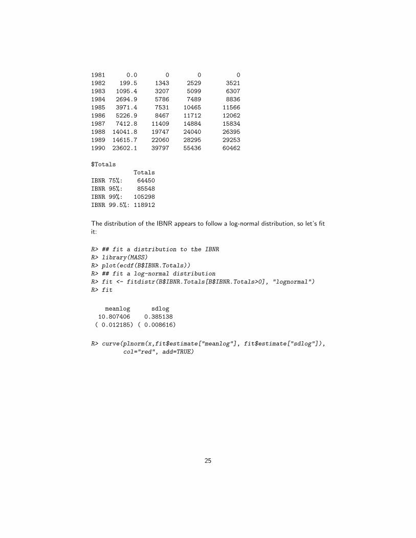
The distribution of the IBNR appears to follow a log-normal distribution, so let’s fitit:

R> ## fit a distribution to the IBNR

R> library(MASS)

R> plot(ecdf(B$IBNR.Totals))

R> ## fit a log-normal distribution

R> fit <- fitdistr(B$IBNR.Totals[B$IBNR.Totals>0], "lognormal")

R> fit

meanlog sdlog

10.807406 0.385138

( 0.012185) ( 0.008616)

R> curve(plnorm(x,fit$estimate["meanlog"], fit$estimate["sdlog"]),

col="red", add=TRUE)

25

0 50000 100000 150000

0.0

0.2

0.4

0.6

0.8

1.0

ecdf(B$IBNR.Totals)

x

Fn(

x)

4.5 Multivariate chain-ladder

The Mack chain ladder technique can be generalized to the multivariate settingwhere multiple reserving triangles are modelled and developed simultaneously. Theadvantage of the multivariate modelling is that correlations among different tri-angles can be modelled, which will lead to more accurate uncertainty assessments.Reserving methods that explicitly model the between-triangle contemporaneous cor-relations can be found in [PS05, MW08b]. Another benefit of multivariate loss re-serving is that structural relationships between triangles can also be reflected, wherethe development of one triangle depends on past losses from other triangles. Forexample, there is generally need for the joint development of the paid and incurredlosses [QM04]. Most of the chain-ladder-based multivariate reserving models can besummarised as sequential seemingly unrelated regressions [Zha10]. We note anotherstrand of multivariate loss reserving builds a hierarchical structure into the model toallow estimation of one triangle to“borrow strength”from other triangles, reflectingthe core insight of actuarial credibility [ZDG12].

Denote Yi,k = (Y(1)i,k , · · · , Y

(N)i,k ) as an N×1 vector of cumulative losses at accident

year i and development year k where (n) refers to the n-th triangle. [Zha10] specifies

26

the model in development period k as:

Yi,k+1 = Ak +Bk · Yi,k + ǫi,k, (5)

where Ak is a column of intercepts and Bk is the development matrix for develop-ment period k. Assumptions for this model are:

E(ǫi,k|Yi,1, · · · , Yi,I+1−k) = 0. (6)

cov(ǫi,k|Yi,1, · · · , Yi,I+1−k) = D(Y−δ/2i,k )ΣkD(Y

−δ/2i,k ). (7)

losses of different accident years are independent. (8)

ǫi,k are symmetrically distributed. (9)

In the above, D is the diagonal operator, and δ is a known positive value thatcontrols how the variance depends on the mean (as weights). This model is referredto as the general multivariate chain ladder [GMCL] in [Zha10]. A important specialcase where Ak = 0 and Bk’s are diagonal is a naive generalization of the chainladder, often referred to as the multivariate chain ladder [MCL] [PS05].

In the following, we first introduce the class "triangles", for which we have definedseveral utility functions. Indeed, any input triangles to the MultiChainLadder

function will be converted to "triangles" internally. We then present loss reservingmethods based on the MCL and GMCL models in turn.

4.6 The "triangles" class

Consider the two liability loss triangles from [MW08b]. It comes as a list of twomatrices :

R> str(liab)

List of 2

$ GeneralLiab: num [1:14, 1:14] 59966 49685 51914 84937 98921 ...

$ AutoLiab : num [1:14, 1:14] 114423 152296 144325 145904 170333 ...

We can convert a list to a "triangles" object using

R> liab2 <- as(liab, "triangles")

R> class(liab2)

[1] "triangles"

attr(,"package")

[1] "ChainLadder"

We can find out what methods are available for this class:

27

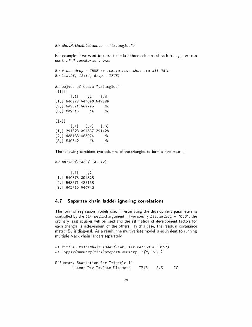
R> showMethods(classes = "triangles")

For example, if we want to extract the last three columns of each triangle, we canuse the "[" operator as follows:

R> # use drop = TRUE to remove rows that are all NA's

R> liab2[, 12:14, drop = TRUE]

An object of class "triangles"

[[1]]

[,1] [,2] [,3]

[1,] 540873 547696 549589

[2,] 563571 562795 NA

[3,] 602710 NA NA

[[2]]

[,1] [,2] [,3]

[1,] 391328 391537 391428

[2,] 485138 483974 NA

[3,] 540742 NA NA

The following combines two columns of the triangles to form a new matrix:

R> cbind2(liab2[1:3, 12])

[,1] [,2]

[1,] 540873 391328

[2,] 563571 485138

[3,] 602710 540742

4.7 Separate chain ladder ignoring correlations

The form of regression models used in estimating the development parameters iscontrolled by the fit.method argument. If we specify fit.method = "OLS", theordinary least squares will be used and the estimation of development factors foreach triangle is independent of the others. In this case, the residual covariancematrix Σk is diagonal. As a result, the multivariate model is equivalent to runningmultiple Mack chain ladders separately.

R> fit1 <- MultiChainLadder(liab, fit.method = "OLS")

R> lapply(summary(fit1)$report.summary, "[", 15, )

$`Summary Statistics for Triangle 1`

Latest Dev.To.Date Ultimate IBNR S.E CV

28

Total 11343397 0.6482 17498658 6155261 427289 0.0694



Total 8759806 0.8093 10823418 2063612 162872 0.0789

$`Summary Statistics for Triangle 1+2`


Total 20103203 0.7098 28322077 8218874 457278 0.0556

In the above, we only show the total reserve estimate for each triangle to reduce theoutput. The full summary including the estimate for each year can be retrieved usingthe usual summary function. By default, the summary function produces reservestatistics for all individual triangles, as well as for the portfolio that is assumed tobe the sum of the two triangles. This behaviour can be changed by supplying theportfolio argument. See the documentation for details.

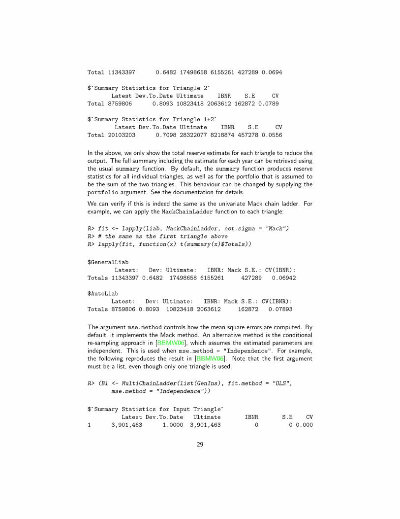
We can verify if this is indeed the same as the univariate Mack chain ladder. Forexample, we can apply the MackChainLadder function to each triangle:

R> fit <- lapply(liab, MackChainLadder, est.sigma = "Mack")

R> # the same as the first triangle above

R> lapply(fit, function(x) t(summary(x)$Totals))

$GeneralLiab

Latest: Dev: Ultimate: IBNR: Mack S.E.: CV(IBNR):

Totals 11343397 0.6482 17498658 6155261 427289 0.06942

$AutoLiab

Latest: Dev: Ultimate: IBNR: Mack S.E.: CV(IBNR):

Totals 8759806 0.8093 10823418 2063612 162872 0.07893

The argument mse.method controls how the mean square errors are computed. Bydefault, it implements the Mack method. An alternative method is the conditionalre-sampling approach in [BBMW06], which assumes the estimated parameters areindependent. This is used when mse.method = "Independence". For example,the following reproduces the result in [BBMW06]. Note that the first argumentmust be a list, even though only one triangle is used.

R> (B1 <- MultiChainLadder(list(GenIns), fit.method = "OLS",

mse.method = "Independence"))

$`Summary Statistics for Input Triangle`


1 3,901,463 1.0000 3,901,463 0 0 0.000

29

2 5,339,085 0.9826 5,433,719 94,634 75,535 0.798

3 4,909,315 0.9127 5,378,826 469,511 121,700 0.259

4 4,588,268 0.8661 5,297,906 709,638 133,551 0.188

5 3,873,311 0.7973 4,858,200 984,889 261,412 0.265

6 3,691,712 0.7223 5,111,171 1,419,459 411,028 0.290

7 3,483,130 0.6153 5,660,771 2,177,641 558,356 0.256

8 2,864,498 0.4222 6,784,799 3,920,301 875,430 0.223

9 1,363,294 0.2416 5,642,266 4,278,972 971,385 0.227

10 344,014 0.0692 4,969,825 4,625,811 1,363,385 0.295

Total 34,358,090 0.6478 53,038,946 18,680,856 2,447,618 0.131

4.8 Multivariate chain ladder using seemingly unrelated re-

gressions

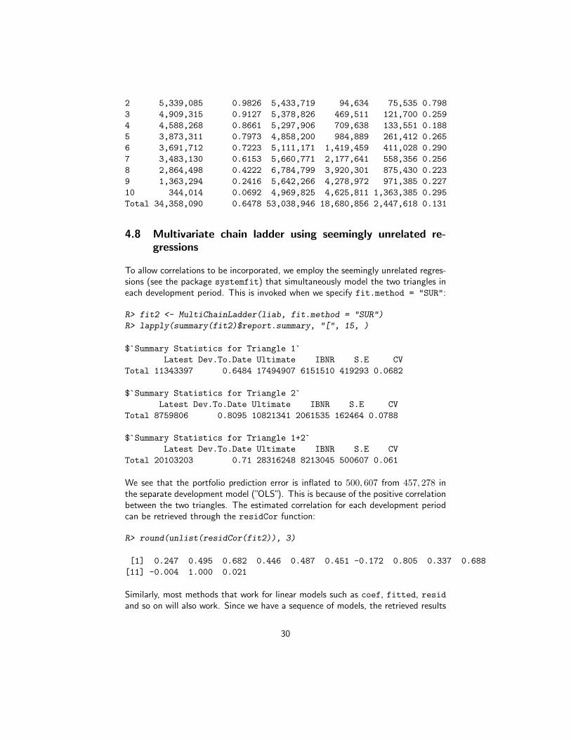
To allow correlations to be incorporated, we employ the seemingly unrelated regres-sions (see the package systemfit) that simultaneously model the two triangles ineach development period. This is invoked when we specify fit.method = "SUR":

R> fit2 <- MultiChainLadder(liab, fit.method = "SUR")

R> lapply(summary(fit2)$report.summary, "[", 15, )



Total 11343397 0.6484 17494907 6151510 419293 0.0682



Total 8759806 0.8095 10821341 2061535 162464 0.0788



Total 20103203 0.71 28316248 8213045 500607 0.061

We see that the portfolio prediction error is inflated to 500, 607 from 457, 278 inthe separate development model (”OLS”). This is because of the positive correlationbetween the two triangles. The estimated correlation for each development periodcan be retrieved through the residCor function:

R> round(unlist(residCor(fit2)), 3)

[1] 0.247 0.495 0.682 0.446 0.487 0.451 -0.172 0.805 0.337 0.688

[11] -0.004 1.000 0.021

Similarly, most methods that work for linear models such as coef, fitted, residand so on will also work. Since we have a sequence of models, the retrieved results

30

from these methods are stored in a list. For example, we can retrieve the estimateddevelopment factors for each period as

R> do.call("rbind", coef(fit2))

eq1_x[[1]] eq2_x[[2]]

[1,] 3.227 2.2224

[2,] 1.719 1.2688

[3,] 1.352 1.1200

[4,] 1.179 1.0665

[5,] 1.106 1.0356

[6,] 1.055 1.0168

[7,] 1.026 1.0097

[8,] 1.015 1.0002

[9,] 1.012 1.0038

[10,] 1.006 0.9994

[11,] 1.005 1.0039

[12,] 1.005 0.9989

[13,] 1.003 0.9997

The smaller-than-one development factors after the 10-th period for the secondtriangle indeed result in negative IBNR estimates for the first several accident yearsin that triangle.

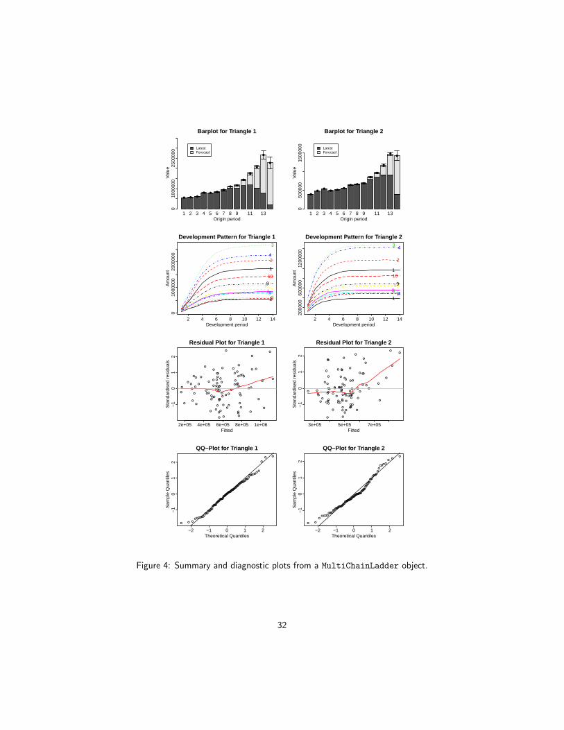
The package also offers the plot method that produces various summary and di-agnostic figures:

R> parold <- par(mfrow = c(4, 2), mar = c(4, 4, 2, 1),

mgp = c(1.3, 0.3, 0), tck = -0.02)

R> plot(fit2, which.triangle = 1:2, which.plot = 1:4)

R> par(parold)

The resulting plots are shown in Figure 4. We use which.triangle to suppressthe plot for the portfolio, and use which.plot to select the desired types of plots.See the documentation for possible values of these two arguments.

4.9 Other residual covariance estimation methods

Internally, the MultiChainLadder calls the systemfit function to fit the regressionmodels period by period. When SUR models are specified, there are several waysto estimate the residual covariance matrix Σk. Available methods are "noDfCor","geomean", "max", and "Theil" with the default as "geomean". The method"Theil" will produce unbiased covariance estimate, but the resulting estimate maynot be positive semi-definite. This is also the estimator used by [MW08b]. However,this method does not work out of the box for the liab data, and is perhaps one

31

1 2 3 4 5 6 7 8 9 11 13

Barplot for Triangle 1

Origin period

Val

ue0

1000

000

2500

000 Latest

Forecast

● ● ●

● ● ●●

● ●

●

●

●

●

●

1 2 3 4 5 6 7 8 9 11 13

Barplot for Triangle 2

Origin period

Val

ue0

5000

0015

0000

0

LatestForecast

●●

●● ●

●● ● ●

●

●

●

●●

2 4 6 8 10 12 14

010

0000

020

0000

0

Development Pattern for Triangle 1

Development period

Am

ount

1234567

89

10

1

2

3

4

2 4 6 8 10 12 14

2000

0060

0000

1200

000

Development Pattern for Triangle 2

Development period

Am

ount

12

3 456

789

101

2

3 4

●

●

●●

●

●

●

●

●

●

●

●

●

●

●

●

●

●

●

●

●

●

●

●

●

●

●

●●

●

●

●

●

●

●

●

●

●

●

●●

●

●

●

●

●

●●

●

●

●

●

●

●

●

●

●

●

●

●

●●

●

●

●

●

●

●

●

●●

●

●

●

●●

●

●

●

●

●●

●

●

●

●

●

●

●

●

●

2e+05 4e+05 6e+05 8e+05 1e+06

−1

01

2

Residual Plot for Triangle 1

Fitted

Sta

ndar

dise

d re

sidu

als

●

●

●●

●

●

●

● ●

●

●

●

●

●

●

●

●

●

●

●●

●

●

●

●

●

●

●●

●

●

●

●

●

●

●

●

●

●

●

●

●

●

●

●

●

●

●

●

●

●

●

● ●

●

●

●

●

●

●

●

●

●

●

●

●

●

●

●

●

●●

●

●

●

●

●

●

●●

●●

●

●

●●

●

●

●

●

●

3e+05 5e+05 7e+05

−1

01

2

Residual Plot for Triangle 2

Fitted

Sta

ndar

dise

d re

sidu

als

●

●

●●

●

●

●

●

●

●

●

●

●

●

●

●

●

●

●

●

●

●

●

●

●

●

●

●●

●

●

●

●

●

●

●

●

●

●

●●

●

●

●

●

●

●●

●

●

●

●

●

●

●

●

●

●

●

●

●●

●

●

●

●

●

●

●

●●

●

●

●

●●

●

●

●

●

●●

●

●

●

●

●

●

●

●

●

−2 −1 0 1 2

−1

01

2

QQ−Plot for Triangle 1

Theoretical Quantiles

Sam

ple

Qua

ntile

s

●

●

●●

●

●

●

●●

●

●

●

●

●

●

●

●

●

●

●●

●

●

●

●

●

●

●●

●

●

●

●

●

●

●

●

●

●

●

●

●

●

●

●

●

●

●

●

●

●

●

●●

●

●

●

●

●

●

●

●

●

●

●

●

●

●

●

●

●●

●

●

●

●

●

●

●●

●●

●

●

●●

●

●

●

●

●

−2 −1 0 1 2

−1

01

2

QQ−Plot for Triangle 2


Sam

ple

Qua

ntile

s

Figure 4: Summary and diagnostic plots from a MultiChainLadder object.

32

of the reasons [MW08b] used extrapolation to get the estimate for the last severalperiods.

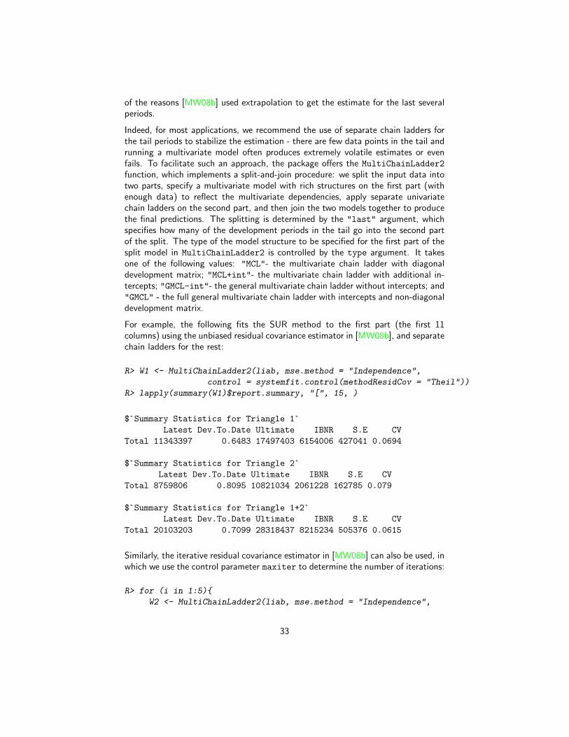
Indeed, for most applications, we recommend the use of separate chain ladders forthe tail periods to stabilize the estimation - there are few data points in the tail andrunning a multivariate model often produces extremely volatile estimates or evenfails. To facilitate such an approach, the package offers the MultiChainLadder2

function, which implements a split-and-join procedure: we split the input data intotwo parts, specify a multivariate model with rich structures on the first part (withenough data) to reflect the multivariate dependencies, apply separate univariatechain ladders on the second part, and then join the two models together to producethe final predictions. The splitting is determined by the "last" argument, whichspecifies how many of the development periods in the tail go into the second partof the split. The type of the model structure to be specified for the first part of thesplit model in MultiChainLadder2 is controlled by the type argument. It takesone of the following values: "MCL"- the multivariate chain ladder with diagonaldevelopment matrix; "MCL+int"- the multivariate chain ladder with additional in-tercepts; "GMCL-int"- the general multivariate chain ladder without intercepts; and"GMCL" - the full general multivariate chain ladder with intercepts and non-diagonaldevelopment matrix.

For example, the following fits the SUR method to the first part (the first 11columns) using the unbiased residual covariance estimator in [MW08b], and separatechain ladders for the rest:

R> W1 <- MultiChainLadder2(liab, mse.method = "Independence",

control = systemfit.control(methodResidCov = "Theil"))

R> lapply(summary(W1)$report.summary, "[", 15, )



Total 11343397 0.6483 17497403 6154006 427041 0.0694



Total 8759806 0.8095 10821034 2061228 162785 0.079



Total 20103203 0.7099 28318437 8215234 505376 0.0615

Similarly, the iterative residual covariance estimator in [MW08b] can also be used, inwhich we use the control parameter maxiter to determine the number of iterations:

R> for (i in 1:5){

W2 <- MultiChainLadder2(liab, mse.method = "Independence",

33

control = systemfit.control(methodResidCov = "Theil", maxiter = i))

print(format(summary(W2)@report.summary[[3]][15, 4:5],

digits = 6, big.mark = ","))

}

IBNR S.E

Total 8,215,234 505,376

IBNR S.E

Total 8,215,357 505,443

IBNR S.E

Total 8,215,362 505,444

IBNR S.E

Total 8,215,362 505,444

IBNR S.E

Total 8,215,362 505,444

R> lapply(summary(W2)$report.summary, "[", 15, )



Total 11343397 0.6483 17497526 6154129 427074 0.0694



Total 8759806 0.8095 10821039 2061233 162790 0.079



Total 20103203 0.7099 28318565 8215362 505444 0.0615

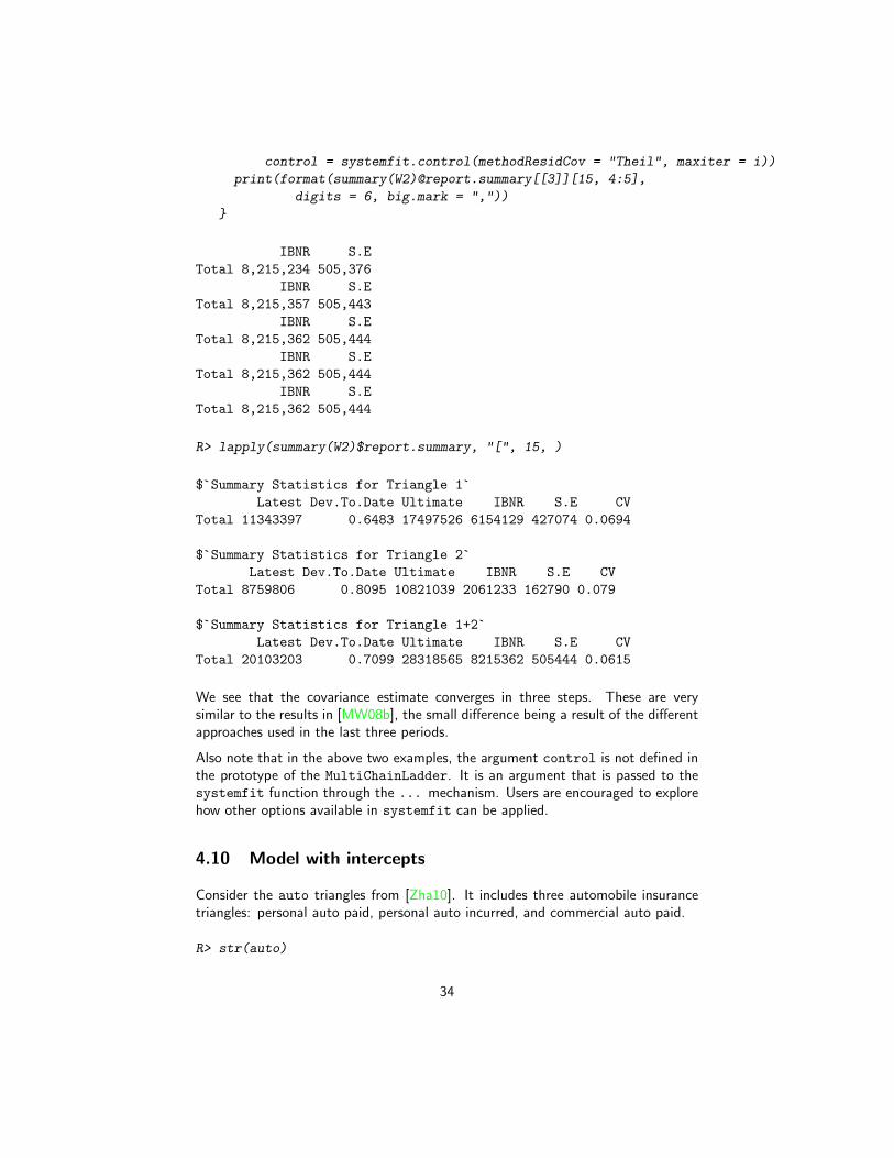
We see that the covariance estimate converges in three steps. These are verysimilar to the results in [MW08b], the small difference being a result of the differentapproaches used in the last three periods.

Also note that in the above two examples, the argument control is not defined inthe prototype of the MultiChainLadder. It is an argument that is passed to thesystemfit function through the ... mechanism. Users are encouraged to explorehow other options available in systemfit can be applied.

4.10 Model with intercepts

Consider the auto triangles from [Zha10]. It includes three automobile insurancetriangles: personal auto paid, personal auto incurred, and commercial auto paid.

R> str(auto)

34

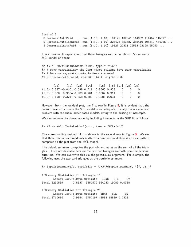
List of 3

$ PersonalAutoPaid : num [1:10, 1:10] 101125 102541 114932 114452 115597 ...

$ PersonalAutoIncurred: num [1:10, 1:10] 325423 323627 358410 405319 434065 ...

$ CommercialAutoPaid : num [1:10, 1:10] 19827 22331 22533 23128 25053 ...

It is a reasonable expectation that these triangles will be correlated. So we run aMCL model on them:

R> f0 <- MultiChainLadder2(auto, type = "MCL")

R> # show correlation- the last three columns have zero correlation

R> # because separate chain ladders are used

R> print(do.call(cbind, residCor(f0)), digits = 3)

[,1] [,2] [,3] [,4] [,5] [,6] [,7] [,8] [,9]

(1,2) 0.327 -0.0101 0.598 0.711 0.8565 0.928 0 0 0

(1,3) 0.870 0.9064 0.939 0.261 -0.0607 0.911 0 0 0

(2,3) 0.198 -0.3217 0.558 0.380 0.3586 0.931 0 0 0

However, from the residual plot, the first row in Figure 5, it is evident that thedefault mean structure in the MCL model is not adequate. Usually this is a commonproblem with the chain ladder based models, owing to the missing of intercepts.

We can improve the above model by including intercepts in the SUR fit as follows:

R> f1 <- MultiChainLadder2(auto, type = "MCL+int")

The corresponding residual plot is shown in the second row in Figure 5. We seethat these residuals are randomly scattered around zero and there is no clear patterncompared to the plot from the MCL model.

The default summary computes the portfolio estimates as the sum of all the trian-gles. This is not desirable because the first two triangles are both from the personalauto line. We can overwrite this via the portfolio argument. For example, thefollowing uses the two paid triangles as the portfolio estimate:

R> lapply(summary(f1, portfolio = "1+3")@report.summary, "[", 11, )



Total 3290539 0.8537 3854572 564033 19089 0.0338



Total 3710614 0.9884 3754197 43583 18839 0.4323

35

●

● ●

●

●

●

●

●●

●

●

●

●

●

●

●

●

●

●

●

●

●

●

●

●

●

●

●

●

●

●

●

●

●

●

●

●

●

●

●

●

●

●

●

●

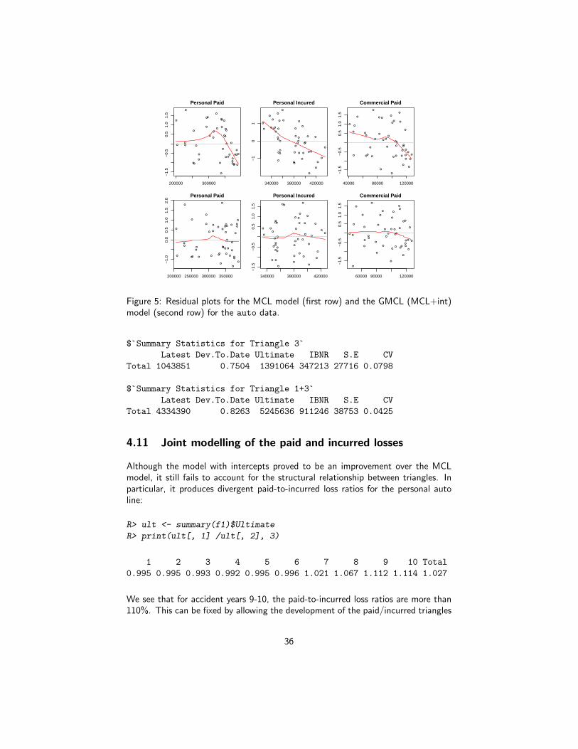
200000 300000

−1.

5−

0.5

0.5

1.0

1.5

Personal Paid

Fitted

●

●

●

●

●

●

●

●●

●

●

●

●

●

●

●

●

●

●

●

●

●

●

●●

●

●

●

●

●

●

●

●

●

●

●

●●

●

●●

●

●

●

●

340000 380000 420000

−1

01

Personal Incured

Fitted

Sta

ndar

dise

d re

sidu

als

●

●

●

●

●

●

●●

●

●

●

●

●

●

●

●

●●

●●

●

●

●

●

●●

●●

●

●

●

●

●

●

●

●

●●

●

●

●

●

●

●

●

40000 80000 120000

−1.

5−

0.5

0.5

1.0

1.5

Commercial Paid

Fitted

●

●

●

●

●

●

●

●● ●

●

●

●

●

●

●

●

●

●

●

●●

●

●

●

●●

●●

●

●

●

●

●

●

●

●

●

●

●

●

●

●

●

●

200000 250000 300000 350000

−1.

00.

00.

51.

01.

52.

0

Personal Paid

●

●

●

●

●

●

●

●

●

●

●

●

●

●

●

●

●

●

●

●

●

●

●

●

●

●

●

●

●

●

●

●

●

●

●

●

●

●

●

●

●

●

●

●

●

340000 380000 420000

−1.

5−

0.5

0.5

1.0

1.5

Personal Incured

Sta

ndar

dise

d re

sidu

als

●●

●

●

●

●

●

●●

●

●

●

●

●

●

●

●

●

●

●

●

●

●

●

●

●

●

●

●

●

●

●

●

● ●

●

●

●

●

●

●

●

●

●

●

60000 80000 120000

−1.

5−

0.5

0.5

1.0

1.5

Commercial Paid

Figure 5: Residual plots for the MCL model (first row) and the GMCL (MCL+int)model (second row) for the auto data.



Total 1043851 0.7504 1391064 347213 27716 0.0798



Total 4334390 0.8263 5245636 911246 38753 0.0425

4.11 Joint modelling of the paid and incurred losses

Although the model with intercepts proved to be an improvement over the MCLmodel, it still fails to account for the structural relationship between triangles. Inparticular, it produces divergent paid-to-incurred loss ratios for the personal autoline:

R> ult <- summary(f1)$Ultimate

R> print(ult[, 1] /ult[, 2], 3)

1 2 3 4 5 6 7 8 9 10 Total

0.995 0.995 0.993 0.992 0.995 0.996 1.021 1.067 1.112 1.114 1.027

We see that for accident years 9-10, the paid-to-incurred loss ratios are more than110%. This can be fixed by allowing the development of the paid/incurred triangles

36

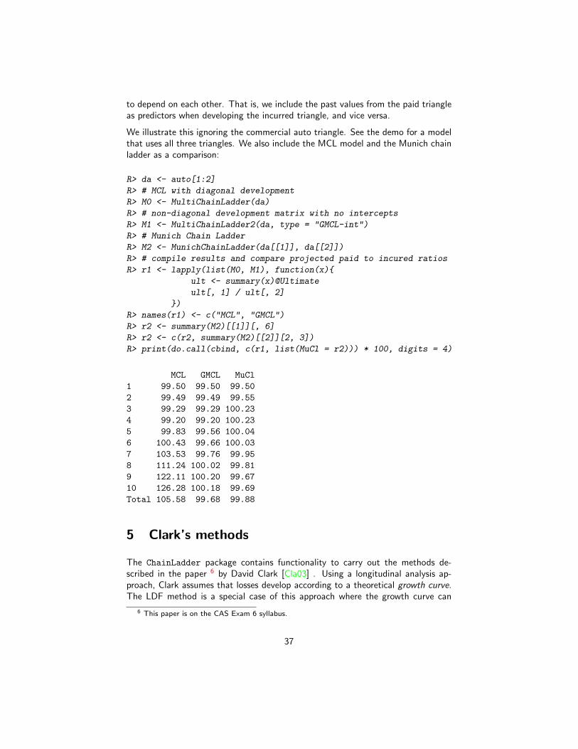
to depend on each other. That is, we include the past values from the paid triangleas predictors when developing the incurred triangle, and vice versa.

We illustrate this ignoring the commercial auto triangle. See the demo for a modelthat uses all three triangles. We also include the MCL model and the Munich chainladder as a comparison:

R> da <- auto[1:2]

R> # MCL with diagonal development

R> M0 <- MultiChainLadder(da)

R> # non-diagonal development matrix with no intercepts

R> M1 <- MultiChainLadder2(da, type = "GMCL-int")

R> # Munich Chain Ladder

R> M2 <- MunichChainLadder(da[[1]], da[[2]])

R> # compile results and compare projected paid to incured ratios

R> r1 <- lapply(list(M0, M1), function(x){

ult <- summary(x)@Ultimate

ult[, 1] / ult[, 2]

})

R> names(r1) <- c("MCL", "GMCL")

R> r2 <- summary(M2)[[1]][, 6]

R> r2 <- c(r2, summary(M2)[[2]][2, 3])

R> print(do.call(cbind, c(r1, list(MuCl = r2))) * 100, digits = 4)

MCL GMCL MuCl

1 99.50 99.50 99.50

2 99.49 99.49 99.55

3 99.29 99.29 100.23

4 99.20 99.20 100.23

5 99.83 99.56 100.04

6 100.43 99.66 100.03

7 103.53 99.76 99.95

8 111.24 100.02 99.81

9 122.11 100.20 99.67

10 126.28 100.18 99.69

Total 105.58 99.68 99.88

5 Clark’s methods

The ChainLadder package contains functionality to carry out the methods de-scribed in the paper 6 by David Clark [Cla03] . Using a longitudinal analysis ap-proach, Clark assumes that losses develop according to a theoretical growth curve.The LDF method is a special case of this approach where the growth curve can

6 This paper is on the CAS Exam 6 syllabus.

37

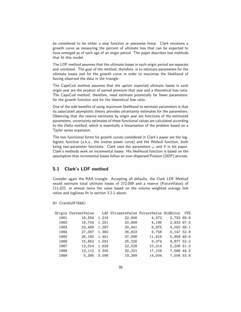
be considered to be either a step function or piecewise linear. Clark envisions agrowth curve as measuring the percent of ultimate loss that can be expected tohave emerged as of each age of an origin period. The paper describes two methodsthat fit this model.

The LDF method assumes that the ultimate losses in each origin period are separateand unrelated. The goal of the method, therefore, is to estimate parameters for theultimate losses and for the growth curve in order to maximize the likelihood ofhaving observed the data in the triangle.

The CapeCod method assumes that the apriori expected ultimate losses in eachorigin year are the product of earned premium that year and a theoretical loss ratio.The CapeCod method, therefore, need estimate potentially far fewer parameters:for the growth function and for the theoretical loss ratio.

One of the side benefits of using maximum likelihood to estimate parameters is thatits associated asymptotic theory provides uncertainty estimates for the parameters.Observing that the reserve estimates by origin year are functions of the estimatedparameters, uncertainty estimates of these functional values are calculated accordingto the Delta method, which is essentially a linearisation of the problem based on aTaylor series expansion.

The two functional forms for growth curves considered in Clark’s paper are the log-logistic function (a.k.a., the inverse power curve) and the Weibull function, bothbeing two-parameter functions. Clark uses the parameters ω and θ in his paper.Clark’s methods work on incremental losses. His likelihood function is based on theassumption that incremental losses follow an over-dispersed Poisson (ODP) process.

5.1 Clark’s LDF method

Consider again the RAA triangle. Accepting all defaults, the Clark LDF Methodwould estimate total ultimate losses of 272,009 and a reserve (FutureValue) of111,022, or almost twice the value based on the volume weighted average linkratios and loglinear fit in section 3.2.1 above.

R> ClarkLDF(RAA)

Origin CurrentValue Ldf UltimateValue FutureValue StdError CV%

1981 18,834 1.216 22,906 4,072 2,792 68.6

1982 16,704 1.251 20,899 4,195 2,833 67.5

1983 23,466 1.297 30,441 6,975 4,050 58.1

1984 27,067 1.360 36,823 9,756 5,147 52.8

1985 26,180 1.451 37,996 11,816 5,858 49.6

1986 15,852 1.591 25,226 9,374 4,877 52.0

1987 12,314 1.829 22,528 10,214 5,206 51.0

1988 13,112 2.305 30,221 17,109 7,568 44.2

1989 5,395 3.596 19,399 14,004 7,506 53.6

38

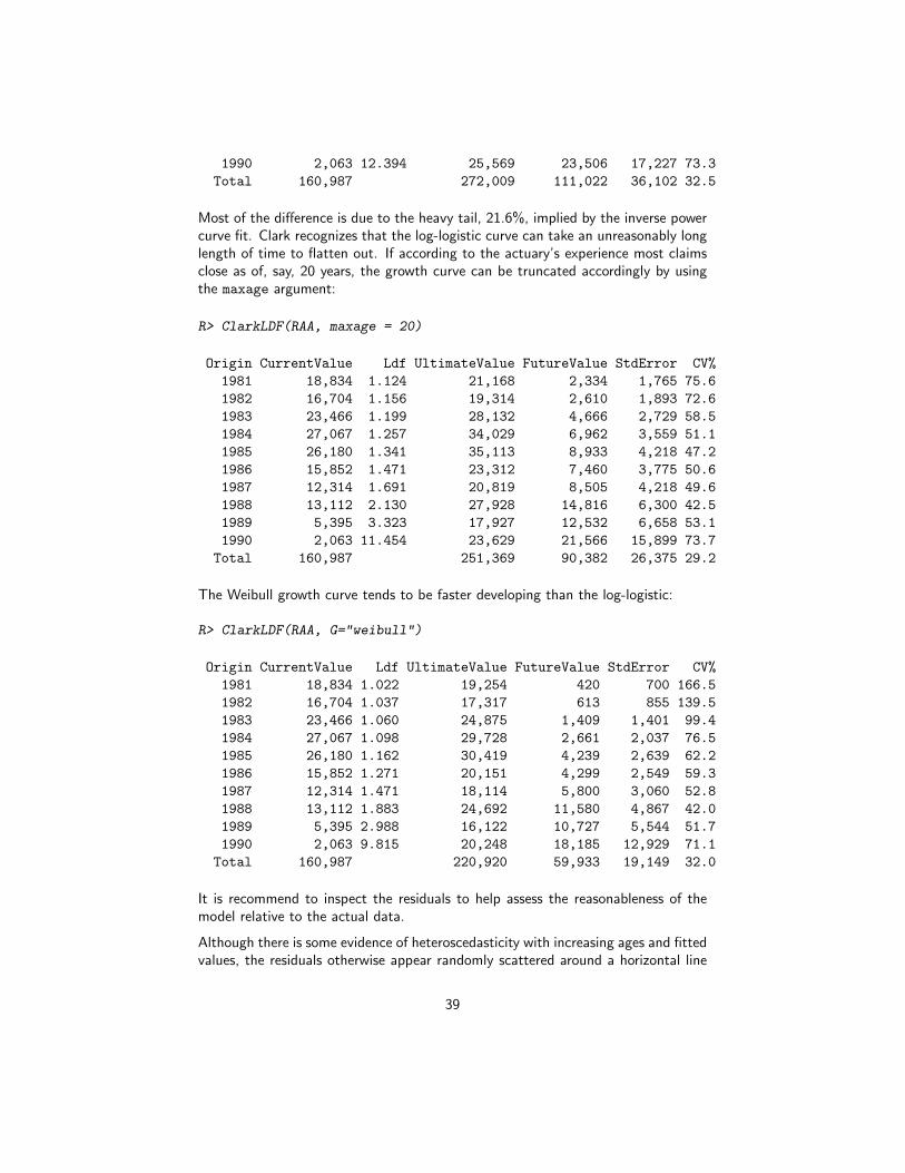
1990 2,063 12.394 25,569 23,506 17,227 73.3

Total 160,987 272,009 111,022 36,102 32.5

Most of the difference is due to the heavy tail, 21.6%, implied by the inverse powercurve fit. Clark recognizes that the log-logistic curve can take an unreasonably longlength of time to flatten out. If according to the actuary’s experience most claimsclose as of, say, 20 years, the growth curve can be truncated accordingly by usingthe maxage argument:

R> ClarkLDF(RAA, maxage = 20)


1981 18,834 1.124 21,168 2,334 1,765 75.6

1982 16,704 1.156 19,314 2,610 1,893 72.6

1983 23,466 1.199 28,132 4,666 2,729 58.5

1984 27,067 1.257 34,029 6,962 3,559 51.1

1985 26,180 1.341 35,113 8,933 4,218 47.2

1986 15,852 1.471 23,312 7,460 3,775 50.6

1987 12,314 1.691 20,819 8,505 4,218 49.6

1988 13,112 2.130 27,928 14,816 6,300 42.5

1989 5,395 3.323 17,927 12,532 6,658 53.1

1990 2,063 11.454 23,629 21,566 15,899 73.7

Total 160,987 251,369 90,382 26,375 29.2

The Weibull growth curve tends to be faster developing than the log-logistic:

R> ClarkLDF(RAA, G="weibull")


1981 18,834 1.022 19,254 420 700 166.5

1982 16,704 1.037 17,317 613 855 139.5

1983 23,466 1.060 24,875 1,409 1,401 99.4

1984 27,067 1.098 29,728 2,661 2,037 76.5

1985 26,180 1.162 30,419 4,239 2,639 62.2

1986 15,852 1.271 20,151 4,299 2,549 59.3

1987 12,314 1.471 18,114 5,800 3,060 52.8

1988 13,112 1.883 24,692 11,580 4,867 42.0

1989 5,395 2.988 16,122 10,727 5,544 51.7

1990 2,063 9.815 20,248 18,185 12,929 71.1

Total 160,987 220,920 59,933 19,149 32.0

It is recommend to inspect the residuals to help assess the reasonableness of themodel relative to the actual data.

Although there is some evidence of heteroscedasticity with increasing ages and fittedvalues, the residuals otherwise appear randomly scattered around a horizontal line

39

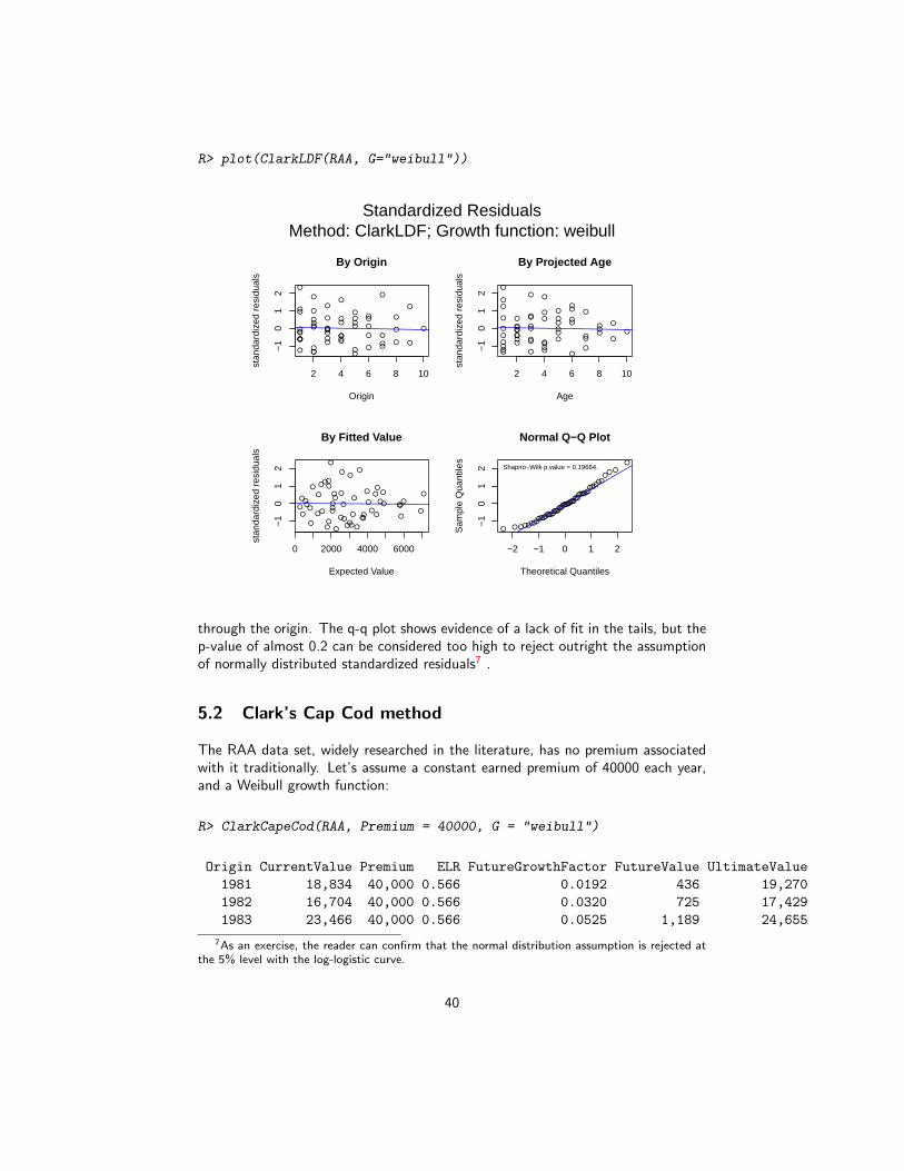
R> plot(ClarkLDF(RAA, G="weibull"))

●

●

●

●

●

●

●●

●

●

●

●●

●

●

●

●●

●●

●

●

●

●

●

●

●

●

●

●

●●

●●

●

●

●

●

●●

●

●

●

●

●

●

●

● ●●

●

●●

●

●

2 4 6 8 10

−1

01

2

By Origin

Origin

stan

dard

ized

res

idua

ls

●

●

●

●

●

●

●●

●

●

●

●●●

●

●

●●

●●

●

●

●

●

●

●

●

●

●

●

●●

●●

●

●

●

●

●●

●

●

●

●

●

●

●

●●●●

●●

●

●

2 4 6 8 10

−1

01

2

By Projected Age

Age

stan

dard

ized

res

idua

ls●

●

●

●

●

●

●●

●

●

●

●●

●

●

●

●●

●●

●

●

●

●

●

●

●

●

●

●

●●

●●

●

●

●

●

●●

●

●

●

●

●

●

●

● ●●●

●●

●

●

0 2000 4000 6000

−1

01

2

By Fitted Value

Expected Value

stan

dard

ized

res

idua

ls

●

●

●

●

●

●

●●

●

●

●

●●

●

●

●

●●

●●

●

●

●

●

●

●

●

●

●

●

●●

●●

●

●

●

●

●●

●

●

●

●

●

●

●

●●●

●

●●

●

●

−2 −1 0 1 2

−1

01

2

Normal Q−Q Plot


Sam

ple

Qua

ntile

sShapiro−Wilk p.value = 0.19684.

Standardized ResidualsMethod: ClarkLDF; Growth function: weibull

through the origin. The q-q plot shows evidence of a lack of fit in the tails, but thep-value of almost 0.2 can be considered too high to reject outright the assumptionof normally distributed standardized residuals7 .

5.2 Clark’s Cap Cod method

The RAA data set, widely researched in the literature, has no premium associatedwith it traditionally. Let’s assume a constant earned premium of 40000 each year,and a Weibull growth function:

R> ClarkCapeCod(RAA, Premium = 40000, G = "weibull")

Origin CurrentValue Premium ELR FutureGrowthFactor FutureValue UltimateValue

1981 18,834 40,000 0.566 0.0192 436 19,270

1982 16,704 40,000 0.566 0.0320 725 17,429

1983 23,466 40,000 0.566 0.0525 1,189 24,655

7As an exercise, the reader can confirm that the normal distribution assumption is rejected atthe 5% level with the log-logistic curve.

40

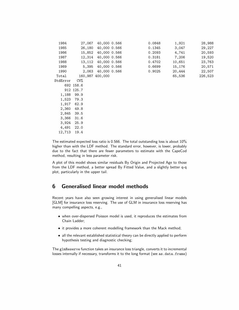
1984 27,067 40,000 0.566 0.0848 1,921 28,988

1985 26,180 40,000 0.566 0.1345 3,047 29,227

1986 15,852 40,000 0.566 0.2093 4,741 20,593

1987 12,314 40,000 0.566 0.3181 7,206 19,520

1988 13,112 40,000 0.566 0.4702 10,651 23,763

1989 5,395 40,000 0.566 0.6699 15,176 20,571

1990 2,063 40,000 0.566 0.9025 20,444 22,507

Total 160,987 400,000 65,536 226,523

StdError CV%

692 158.6

912 125.7

1,188 99.9

1,523 79.3

1,917 62.9

2,360 49.8

2,845 39.5

3,366 31.6

3,924 25.9

4,491 22.0

12,713 19.4

The estimated expected loss ratio is 0.566. The total outstanding loss is about 10%higher than with the LDF method. The standard error, however, is lower, probablydue to the fact that there are fewer parameters to estimate with the CapeCodmethod, resulting in less parameter risk.

A plot of this model shows similar residuals By Origin and Projected Age to thosefrom the LDF method, a better spread By Fitted Value, and a slightly better q-qplot, particularly in the upper tail.

6 Generalised linear model methods

Recent years have also seen growing interest in using generalised linear models[GLM] for insurance loss reserving. The use of GLM in insurance loss reserving hasmany compelling aspects, e.g.,

• when over-dispersed Poisson model is used, it reproduces the estimates fromChain Ladder;

• it provides a more coherent modelling framework than the Mack method;

• all the relevant established statistical theory can be directly applied to performhypothesis testing and diagnostic checking;

The glmReserve function takes an insurance loss triangle, converts it to incrementallosses internally if necessary, transforms it to the long format (see as.data.frame)

41

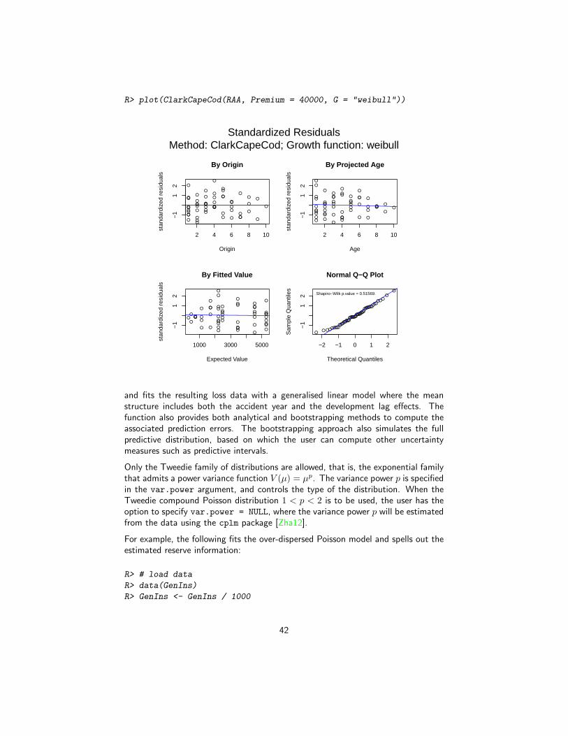
R> plot(ClarkCapeCod(RAA, Premium = 40000, G = "weibull"))

●

●

●

●

●●

●

●

●

●

●●

● ●

●

●

●

●

●

●

●

●●

●

●

●●

●

●

●

●

●

● ●

●

●●

●

●

●

●

●

●

●

●

●

●

●●● ● ●

●

●●

2 4 6 8 10

−1

12

By Origin

Origin

stan

dard

ized

res

idua

ls

●

●

●

●

●●

●

●

●

●

●●

●●

●

●

●

●

●

●

●

●●

●

●

●●

●

●

●

●

●

●●

●

●●●

●

●

●

●

●

●

●

●

●

●● ●●●

●

●●

2 4 6 8 10

−1

12

By Projected Age

Age

stan

dard

ized

res

idua

ls●

●

●

●

●●

●

●

●

●

●●

●●

●

●

●

●

●

●

●

●●

●

●

●●

●

●

●

●

●

●●

●

●●●

●

●

●

●

●

●

●

●

●

●●●●●

●

●●

1000 3000 5000

−1

12

By Fitted Value

Expected Value

stan

dard

ized

res

idua

ls

●

●

●

●

●●

●

●

●

●

●●

●●

●

●

●

●

●

●

●

●●

●

●

●●

●

●

●

●

●

● ●

●

●●

●

●

●

●

●

●

●

●

●

●

●●● ●●

●

●●

−2 −1 0 1 2

−1

12

Normal Q−Q Plot


Sam

ple

Qua

ntile

sShapiro−Wilk p.value = 0.51569.

Standardized ResidualsMethod: ClarkCapeCod; Growth function: weibull

and fits the resulting loss data with a generalised linear model where the meanstructure includes both the accident year and the development lag effects. Thefunction also provides both analytical and bootstrapping methods to compute theassociated prediction errors. The bootstrapping approach also simulates the fullpredictive distribution, based on which the user can compute other uncertaintymeasures such as predictive intervals.

Only the Tweedie family of distributions are allowed, that is, the exponential familythat admits a power variance function V (µ) = µp. The variance power p is specifiedin the var.power argument, and controls the type of the distribution. When theTweedie compound Poisson distribution 1 < p < 2 is to be used, the user has theoption to specify var.power = NULL, where the variance power p will be estimatedfrom the data using the cplm package [Zha12].

For example, the following fits the over-dispersed Poisson model and spells out theestimated reserve information:

R> # load data

R> data(GenIns)

R> GenIns <- GenIns / 1000

42

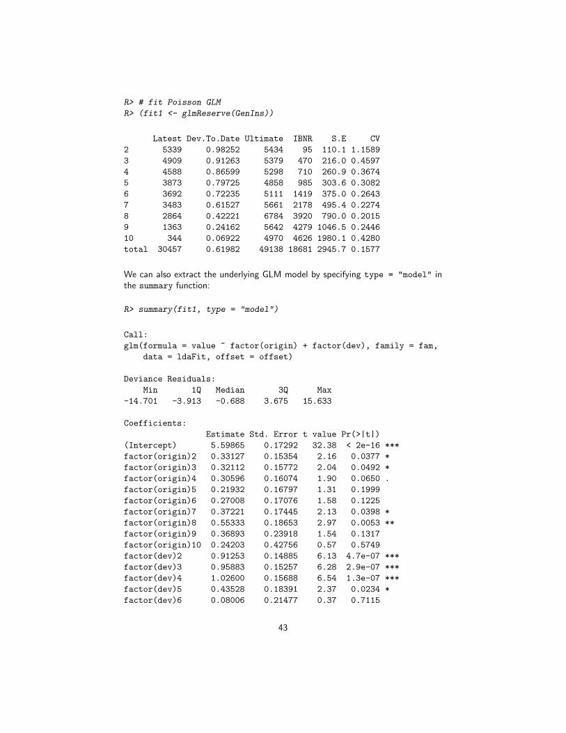
R> # fit Poisson GLM

R> (fit1 <- glmReserve(GenIns))


2 5339 0.98252 5434 95 110.1 1.1589

3 4909 0.91263 5379 470 216.0 0.4597

4 4588 0.86599 5298 710 260.9 0.3674

5 3873 0.79725 4858 985 303.6 0.3082

6 3692 0.72235 5111 1419 375.0 0.2643

7 3483 0.61527 5661 2178 495.4 0.2274

8 2864 0.42221 6784 3920 790.0 0.2015

9 1363 0.24162 5642 4279 1046.5 0.2446

10 344 0.06922 4970 4626 1980.1 0.4280

total 30457 0.61982 49138 18681 2945.7 0.1577

We can also extract the underlying GLM model by specifying type = "model" inthe summary function:

R> summary(fit1, type = "model")

Call:

glm(formula = value ~ factor(origin) + factor(dev), family = fam,

data = ldaFit, offset = offset)

Deviance Residuals:

Min 1Q Median 3Q Max

-14.701 -3.913 -0.688 3.675 15.633

Coefficients:

Estimate Std. Error t value Pr(>|t|)

(Intercept) 5.59865 0.17292 32.38 < 2e-16 ***

factor(origin)2 0.33127 0.15354 2.16 0.0377 *

factor(origin)3 0.32112 0.15772 2.04 0.0492 *

factor(origin)4 0.30596 0.16074 1.90 0.0650 .

factor(origin)5 0.21932 0.16797 1.31 0.1999

factor(origin)6 0.27008 0.17076 1.58 0.1225

factor(origin)7 0.37221 0.17445 2.13 0.0398 *

factor(origin)8 0.55333 0.18653 2.97 0.0053 **

factor(origin)9 0.36893 0.23918 1.54 0.1317

factor(origin)10 0.24203 0.42756 0.57 0.5749

factor(dev)2 0.91253 0.14885 6.13 4.7e-07 ***

factor(dev)3 0.95883 0.15257 6.28 2.9e-07 ***

factor(dev)4 1.02600 0.15688 6.54 1.3e-07 ***

factor(dev)5 0.43528 0.18391 2.37 0.0234 *

factor(dev)6 0.08006 0.21477 0.37 0.7115

43

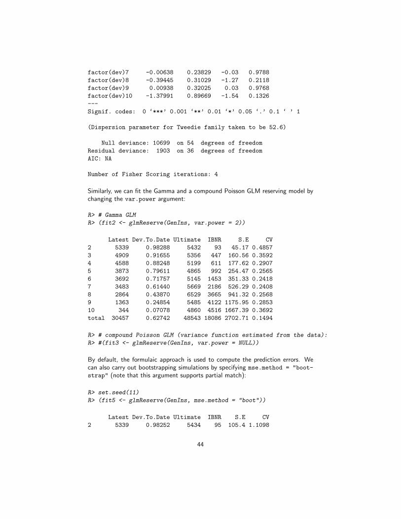
factor(dev)7 -0.00638 0.23829 -0.03 0.9788

factor(dev)8 -0.39445 0.31029 -1.27 0.2118

factor(dev)9 0.00938 0.32025 0.03 0.9768

factor(dev)10 -1.37991 0.89669 -1.54 0.1326

---

Signif. codes: 0 ‘***’ 0.001 ‘**’ 0.01 ‘*’ 0.05 ‘.’ 0.1 ‘ ’ 1

(Dispersion parameter for Tweedie family taken to be 52.6)

Null deviance: 10699 on 54 degrees of freedom

Residual deviance: 1903 on 36 degrees of freedom

AIC: NA

Number of Fisher Scoring iterations: 4

Similarly, we can fit the Gamma and a compound Poisson GLM reserving model bychanging the var.power argument:

R> # Gamma GLM

R> (fit2 <- glmReserve(GenIns, var.power = 2))


2 5339 0.98288 5432 93 45.17 0.4857

3 4909 0.91655 5356 447 160.56 0.3592

4 4588 0.88248 5199 611 177.62 0.2907

5 3873 0.79611 4865 992 254.47 0.2565

6 3692 0.71757 5145 1453 351.33 0.2418

7 3483 0.61440 5669 2186 526.29 0.2408

8 2864 0.43870 6529 3665 941.32 0.2568

9 1363 0.24854 5485 4122 1175.95 0.2853

10 344 0.07078 4860 4516 1667.39 0.3692

total 30457 0.62742 48543 18086 2702.71 0.1494

R> # compound Poisson GLM (variance function estimated from the data):

R> #(fit3 <- glmReserve(GenIns, var.power = NULL))

By default, the formulaic approach is used to compute the prediction errors. Wecan also carry out bootstrapping simulations by specifying mse.method = "boot-

strap" (note that this argument supports partial match):

R> set.seed(11)

R> (fit5 <- glmReserve(GenIns, mse.method = "boot"))


2 5339 0.98252 5434 95 105.4 1.1098

44

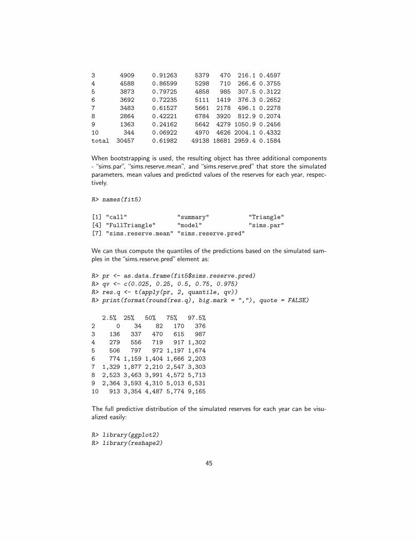
3 4909 0.91263 5379 470 216.1 0.4597

4 4588 0.86599 5298 710 266.6 0.3755

5 3873 0.79725 4858 985 307.5 0.3122

6 3692 0.72235 5111 1419 376.3 0.2652

7 3483 0.61527 5661 2178 496.1 0.2278

8 2864 0.42221 6784 3920 812.9 0.2074

9 1363 0.24162 5642 4279 1050.9 0.2456

10 344 0.06922 4970 4626 2004.1 0.4332

total 30457 0.61982 49138 18681 2959.4 0.1584

When bootstrapping is used, the resulting object has three additional components- “sims.par”, “sims.reserve.mean”, and “sims.reserve.pred” that store the simulatedparameters, mean values and predicted values of the reserves for each year, respec-tively.

R> names(fit5)

[1] "call" "summary" "Triangle"

[4] "FullTriangle" "model" "sims.par"

[7] "sims.reserve.mean" "sims.reserve.pred"

We can thus compute the quantiles of the predictions based on the simulated sam-ples in the“sims.reserve.pred”element as:

R> pr <- as.data.frame(fit5$sims.reserve.pred)

R> qv <- c(0.025, 0.25, 0.5, 0.75, 0.975)

R> res.q <- t(apply(pr, 2, quantile, qv))

R> print(format(round(res.q), big.mark = ","), quote = FALSE)

2.5% 25% 50% 75% 97.5%

2 0 34 82 170 376

3 136 337 470 615 987

4 279 556 719 917 1,302

5 506 797 972 1,197 1,674

6 774 1,159 1,404 1,666 2,203

7 1,329 1,877 2,210 2,547 3,303

8 2,523 3,463 3,991 4,572 5,713

9 2,364 3,593 4,310 5,013 6,531

10 913 3,354 4,487 5,774 9,165

The full predictive distribution of the simulated reserves for each year can be visu-alized easily:

R> library(ggplot2)

R> library(reshape2)

45

R> prm <- melt(pr)

R> names(prm) <- c("year", "reserve")

R> gg <- ggplot(prm, aes(reserve))

R> gg <- gg + geom_density(aes(fill = year), alpha = 0.3) +

facet_wrap(~year, nrow = 2, scales = "free") +

theme(legend.position = "none")

R> print(gg)

7 One year claims development result

The stochastic claims reserving methods considered above predict the lower (un-known) triangle and assess the uncertainty of this prediction. For instance, Mack’suncertainty formula quantifies the total prediction uncertainty of the chain-ladderpredictor over the entire run-off of the outstanding claims. Modern solvency consid-erations, such as Solvency II, require a second view of claims reserving uncertainty.This second view is a short-term view because it requires assessments of the one-year changes of the claims predictions when one updates the available informationat the end of each accounting year. At time t ≥ n we have information

Dt = {Ci,k; i+ k ≤ t+ 1} .

This motivates the following sequence of predictors for the ultimate claim Ci,K attimes t ≥ n

C(t)i,K = E[Ci,K |Dt].

The one year claims development results (CDR), see Merz-Wuthrich [MW08a,MW14], consider the changes in these one year updates, that is,

CDRi,t+1 = C(t)i,K − C

(t+1)i,K .

The tower property of conditional expectation implies that the CDRs are on average0, that is, E[CDRi,t+1|Dt] = 0 and the Merz-Wuthrich formula [MW08a, MW14]assesses the uncertainty of these predictions measured by the following conditionalmean square error of prediction (MSEP)

msepCDRi,t+1|Dt(0) = E

[(CDRi,t+1 − 0)

2∣∣∣Dt

].

The major difficulty in the evaluation of the conditional MSEP is the quantificationof parameter estimation uncertainty.

7.1 CDR functions

The one year claims development result (CDR) can be estimate via the generic CDRfunction for objects of MackChainLadder and BootChainLadder.

46

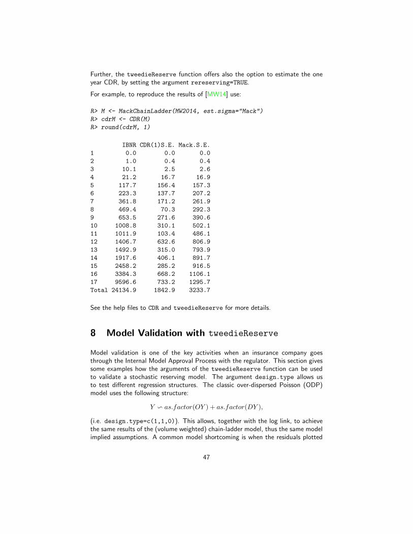
Further, the tweedieReserve function offers also the option to estimate the oneyear CDR, by setting the argument rereserving=TRUE.

For example, to reproduce the results of [MW14] use:

R> M <- MackChainLadder(MW2014, est.sigma="Mack")

R> cdrM <- CDR(M)

R> round(cdrM, 1)

IBNR CDR(1)S.E. Mack.S.E.

1 0.0 0.0 0.0

2 1.0 0.4 0.4

3 10.1 2.5 2.6

4 21.2 16.7 16.9

5 117.7 156.4 157.3

6 223.3 137.7 207.2

7 361.8 171.2 261.9

8 469.4 70.3 292.3

9 653.5 271.6 390.6

10 1008.8 310.1 502.1

11 1011.9 103.4 486.1

12 1406.7 632.6 806.9

13 1492.9 315.0 793.9

14 1917.6 406.1 891.7

15 2458.2 285.2 916.5

16 3384.3 668.2 1106.1

17 9596.6 733.2 1295.7

Total 24134.9 1842.9 3233.7

See the help files to CDR and tweedieReserve for more details.

8 Model Validation with tweedieReserve

Model validation is one of the key activities when an insurance company goesthrough the Internal Model Approval Process with the regulator. This section givessome examples how the arguments of the tweedieReserve function can be usedto validate a stochastic reserving model. The argument design.type allows usto test different regression structures. The classic over-dispersed Poisson (ODP)model uses the following structure:

Y ∽ as.factor(OY ) + as.factor(DY ),

(i.e. design.type=c(1,1,0)). This allows, together with the log link, to achievethe same results of the (volume weighted) chain-ladder model, thus the same modelimplied assumptions. A common model shortcoming is when the residuals plotted

47

by calendar period start to show a pattern, which chain-ladder isn’t capable tomodel. In order to overcome this, the user could be then interested to change theregression structure in order to try to strip out these patterns [GS05]. For example,a regression structure like:

Y ∽ as.factor(DY ) + as.factor(CY ),

i.e. design.type=c(0,1,1) could be considered instead. This approach returnsthe same results of the arithmetic separation method, modelling explicitly inflationparameters between consequent calendar periods. Another interesting assumptionis the assumed underlying distribution. The ODP model assumes the following:

Pi,j ∽ ODP (mi,j , φ ·mi,j),

which is a particular case of a Tweedie distribution, with p parameter equals to 1.Generally speaking, for any random variable Y that obeys a Tweedie distribution,the variance V[Y ] relates to the mean E[Y ] by the following law:

V[Y ] = a · E[Y ]p,

where a and p are positive constants. The user is able to test different p val-ues through the var.power function argument. Besides, in order to validate theTweedie’s p parameter, it could be interesting to plot the likelihood profile at definedp values (through the p.check argument) for a given a dataset and a regressionstructure. This could be achieved setting the p.optim=TRUE argument, as follows:

R> p_profile <- tweedieReserve(MW2008, p.optim=TRUE,

p.check=c(0,1.1,1.2,1.3,1.4,1.5,2,3),

design.type=c(0,1,1),

rereserving=FALSE,

bootstrap=0,

progressBar=FALSE)

R> # 0 1.1 1.2 1.3 1.4 1.5 2 3

R> # ........Done.

R> # MLE of p is between 0 and 1, which is impossible.

R> # Instead, the MLE of p has been set to NA .

R> # Please check your data and the call to tweedie.profile().

R> # Error in if ((xi.max == xi.vec[1]) | (xi.max == xi.vec[length(xi.vec)])) { :

R> # missing value where TRUE/FALSE needed

This example shows, see Figure 6, that the MLE of p seems to be between 0 and1, which is not possible as Tweedie models aren’t defined for 0 < p < 1, thus theError message. But, despite this, we can conclude that overall a value p=1 could bereasonable for this dataset and the chosen regression function, as anyway it seemsto be near the MLE. Other sensitivities could be run on:

• Bootstrap type (parametric / semi-parametric), via the bootstrap argument

48

0.0 0.5 1.0 1.5 2.0 2.5 3.0

−640

−620

−600

−580

−560

−540

−520

p index

L

Figure 6: Likelihood profile of regression structure

• Bias adjustment (if using semi-parametric bootstrap), via the boot.adj ar-gument

Please refer to help(tweedieReserve) for additional information.

9 Using ChainLadder with RExcel and SWord

The ChainLadder package comes with example files which demonstrate how itsfunctions can be embedded in Excel and Word using the statconn interface[BN07].

The spreadsheet is located in the Excel folder of the package. The R command

R> system.file("Excel", package="ChainLadder")

will tell you the exact path to the directory. To use the spreadsheet you will needthe RExcel-Add-in [BN07]. The package also provides an example SWord file,demonstrating how the functions of the package can be integrated into a MS Wordfile via SWord [BN07]. Again you find the Word file via the command:

R> system.file("SWord", package="ChainLadder")

The package comes with several demos to provide you with an overview of thepackage functionality, see

R> demo(package="ChainLadder")

49

http://rcom.univie.ac.at/

10 Further resources

Other useful documents and resources to get started with R in the context ofactuarial work:

• Introduction to R for Actuaries [DS06].

• Computational Actuarial Science with R [Cha14]

• Modern Actuarial Risk Theory – Using R [KGDD01]

• An Actuarial Toolkit [MSH+06].

• Mailing list R-SIG-insurance8: Special Interest Group on using R in actuarialscience and insurance

10.1 Other insurance related R packages

Below is a list of further R packages in the context of insurance. The list is byno-means complete, and the CRAN Task Views ’Empirical Finance’ and ProbabilityDistributions will provide links to additional resources. Please feel free to contactus with items to be added to the list.

• cplm: Likelihood-based and Bayesian methods for fitting Tweedie compoundPoisson linear models [Zha12].

• lossDev: A Bayesian time series loss development model. Features includeskewed-t distribution with time-varying scale parameter, Reversible JumpMCMC for determining the functional form of the consumption path, anda structural break in this path [LS11].

• favir: Formatted Actuarial Vignettes in R. FAViR lowers the learning curveof the R environment. It is a series of peer-reviewed Sweave papers that usea consistent style [Esc11].

• actuar: Loss distributions modelling, risk theory (including ruin theory), sim-ulation of compound hierarchical models and credibility theory [DGP08].

• fitdistrplus: Help to fit of a parametric distribution to non-censored orcensored data [DMPDD10].

• mondate: R package to keep track of dates in terms of months [Mur11].

• lifecontingencies: Package to perform actuarial evaluation of life contin-gencies [Spe11].

• MRMR: Multivariate Regression Models for Reserving [Fan13].

8https://stat.ethz.ch/mailman/listinfo/r-sig-insurance

50

https://stat.ethz.ch/mailman/listinfo/r-sig-insurance

http://cran.r-project.org/web/views/Finance.html

http://cran.r-project.org/web/views/Distributions.html

http://cran.r-project.org/web/views/Distributions.html

mailto:[email protected]

https://stat.ethz.ch/mailman/listinfo/r-sig-insurance

10.2 Presentations

Over the years the contributors of the ChainLadder package have given numerouspresentations and most of those are still available on-line:

• A re-reserving algorithm to derive the one-year reserve risk view, R in Insur-ance, London, Alessandro Carrato, 2013.

• Bayesian Hierarchical Models in Property-Casualty Insurance, Wayne Zhang,2011

• ChainLadder at the Predictive Modelling Seminar, Institute of Actuaries,November 2010, Markus Gesmann, 2011

• Reserve variability calculations, CAS spring meeting, San Diego, Jimmy CurcioJr., Markus Gesmann and Wayne Zhang, 2010

• The ChainLadder package, working with databases and MS Office interfaces,presentation at the ”R you ready?”workshop , Institute of Actuaries, MarkusGesmann, 2009

• The ChainLadder package, London R user group meeting, Markus Gesmann,2009

• Introduction to R, Loss Reserving with R, Stochastic Reserving and ModellingSeminar, Institute of Actuaries, Markus Gesmann, 2008

• Loss Reserving with R , CAS meeting, Vincent Goulet, Markus Gesmann andDaniel Murphy, 2008

• The ChainLadder package R-user conference Dortmund, Markus Gesmann,2008

10.3 Further reading

Other papers and presentations which cited ChainLadder : [Orr07], [Nic09], [Zha10],[MNNV10], [Sch10], [MNV10], [Esc11], [Spe11]

11 Training and consultancy

Please contact us if you would like to discuss tailored training or consultancy.

51

http://chainladder.googlecode.com/files/ChainLadder_Markus_20010Nov10.pdf

http://chainladder.googlecode.com/files/ChainLadder_Markus_20010Nov10.pdf

http://chainladder.googlecode.com/files/CAS-Spring-Meeting-2010-C21.pdf

http://chainladder.googlecode.com/files/ChainLadder_Markus_20090724.pdf

http://chainladder.googlecode.com/files/ChainLadder_Markus_20090724.pdf

http://chainladder.googlecode.com/files/ChainLadder_at_London_R_User_Group_20090331.pdf

http://chainladder.googlecode.com/files/Introduction_to_R_20081203.pdf

http://chainladder.googlecode.com/files/Loss_Reserving_in_R_20081203.pdf

http://chainladder.googlecode.com/files/LossReserving%20with%20R%2020081113.pdf

http://chainladder.googlecode.com/files/ChainLadderPackage_Dortmund_2008.pdf

mailto:[email protected]

References

[BBMW06] M. Buchwalder, H. Buhlmann, M. Merz, and M.V Wuthrich. Themean square error of prediction in the chain ladder reserving method(mack and murphy revisited). North American Actuarial Journal,36:521–542, 2006.

[BN07] Thomas Baier and Erich Neuwirth. Excel :: Com :: R. ComputationalStatistics, 22(1), April 2007. Physica Verlag.

[Cha14] Arthur Charpentier, editor. Computational Actuarial Science with R.Chapman and Hall/CRC, 2014.

[Cla03] David R. Clark. LDF Curve-Fitting and Stochastic Reserving: A Max-imum Likelihood Approach. Casualty Actuarial Society, 2003. CASFall Forum.

[DGP08] C Dutang, V. Goulet, and M. Pigeon. actuar: An R package foractuarial science. Journal of Statistical Software, 25(7), 2008.

[DMPDD10] Marie Laure Delignette-Muller, Regis Pouillot, Jean-Baptiste Denis,and Christophe Dutang. fitdistrplus: help to fit of a parametric dis-tribution to non-censored or censored data, 2010. R package version0.1-3.

[DS06] Nigel De Silva. An introduction to r: Examples for actuaries. http://toolkit.pbwiki.com/RToolkit, 2006.

[Esc11] Benedict Escoto. favir: Formatted Actuarial Vignettes in R, 0.5-1edition, January 2011.

[Fan13] Brian A. Fannin. MRMR: Multivariate Regression Models for Reserv-ing, 2013. R package version 0.1.3.

[GBB+09] Brian Gravelsons, Matthew Ball, Dan Beard, Robert Brooks, NaomiCouchman, Brian Gravelsons, Charlie Kefford, Darren Michaels,Patrick Nolan, Gregory Overton, Stephen Robertson-Dunn, Emil-iano Ruffini, Graham Sandhouse, Jerome Schilling, Dan Sykes,Peter Taylor, Andy Whiting, Matthew Wilde, and John Wilson.B12: Uk asbestos working party update 2009. http://www.

actuaries.org.uk/research-and-resources/documents/

b12-uk-asbestos-working-party-update-2009-5mb, October2009. Presented at the General Insurance Convention.

[Ges14] Markus Gesmann. Claims reserving and IBNR. In ComputationalActuarial Science with R, pages 656–Page. Chapman and Hall/CRC,2014.

52

http://toolkit.pbwiki.com/RToolkit

http://toolkit.pbwiki.com/RToolkit

http://www.actuaries.org.uk/research-and-resources/documents/b12-uk-asbestos-working-party-update-2009-5mb



[GMZ14] Markus Gesmann, Dan Murphy, and Wayne Zhang. ChainLadder:Mack-, Bootstrap and Munich-chain-ladder methods for insuranceclaims reserving, 2014. R package version 0.2.0.

[GS05] Gigante and Sigalotti. Model risk in claims reserving with glm. Gior-nale dell IIA, LXVIII:55 – 87, 2005.

[KGDD01] R. Kaas, M. Goovaerts, J. Dhaene, and M. Denuit. Modern actuarialrisk theory. Kluwer Academic Publishers, Dordrecht, 2001.

[LFK+02] Graham Lyons, Will Forster, Paul Kedney, Ryan Warren, and HelenWilkinson. Claims Reserving Working Party paper. Institute of Actu-aries, October 2002.

[LS11] Christopher W. Laws and Frank A. Schmid. lossDev: Robust LossDevelopment Using MCMC, 2011. R package version 3.0.0-1.

[Mac93] Thomas Mack. Distribution-free calculation of the standard error ofchain ladder reserve estimates. ASTIN Bulletin, 23:213–225, 1993.

[Mac99] Thomas Mack. The standard error of chain ladder reserve estimates:Recursive calculation and inclusion of a tail factor. Astin Bulletin, Vol.29(2):361 – 266, 1999.

[Mic02] Darren Michaels. APH: how the love carnal andsilicone implants nearly destroyed Lloyd’s (slides).http://www.actuaries.org.uk/research-and-

resources/documents/aph-how-love-carnal-and-silicone-

implants-nearly-destroyed-lloyds-s, December 2002. Pre-sented at the Younger Members’ Convention.

[MNNV10] Maria Dolores Martinez Miranda, Bent Nielsen, Jens Perch Nielsen,and Richard Verrall. Cash flow simulation for a model of outstand-ing liabilities based on claim amounts and claim numbers. CASS,September 2010.

[MNV10] Maria Dolores Martinez Miranda, Jens Perch Nielsen, and RichardVerrall. Double Chain Ladder. ASTIN, Colloqiua Madrid edition,2010.

[MSH+06] Trevor Maynard, Nigel De Silva, Richard Holloway, Markus Gesmann,Sie Lau, and John Harnett. An actuarial toolkit. introducing TheToolkit Manifesto. http://www.actuaries.org.uk/sites/all/

files/documents/pdf/actuarial-toolkit.pdf, 2006. GeneralInsurance Convention.

[Mur94] Daniel Murphy. Unbiased loss development factors. PCAS, 81:154 –222, 1994.

53

http://www.actuaries.org.uk/research-and-resources/documents/aph-how-love-carnal-and-silicone-implants-nearly-destroyed-lloyds-s



http://www.actuaries.org.uk/sites/all/files/documents/pdf/actuarial-toolkit.pdf

http://www.actuaries.org.uk/sites/all/files/documents/pdf/actuarial-toolkit.pdf

[Mur11] Daniel Murphy. mondate: Keep track of dates in terms of months,2011. R package version 0.9.8.24.

[MW08a] Michael Merz and Mario V. Wuthrich. Modelling the claims devel-opment result for solvency purposes. CAS E-Forum, Fall:542–568,2008.

[MW08b] Michael Merz and Mario V. Wuthrich. Prediction error of the mul-tivariate chain ladder reserving method. North American ActuarialJournal, 12:175–197, 2008.

[MW14] Michael Merz and Mario V. Wuthrich. Claims run-off uncertainty: thefull picture. SSRN Manuscript, 2524352, 2014.

[Nic09] Luke Nichols. Multimodel Inference for Reserving. Australian Pruden-tial Regulation Authority (APRA), December 2009.

[Orr07] James Orr. A Simple Multi-State Reserving Model. ASTIN, ColloqiuaOrlando edition, 2007.

[Orr12] James Orr. GIROC reserving research workstream. Institute of Actu-aries, November 2012.

[PR02] P.D.England and R.J.Verrall. Stochastic claims reserving in generalinsurance. British Actuarial Journal, 8:443–544, 2002.

[PS05] Carsten Prohl and Klaus D. Schmidt. Multivariate chain-ladder. Dres-dner Schriften zur Versicherungsmathematik, 2005.

[QM04] Gerhard Quarg and Thomas Mack. Munich chain ladder. Munich ReGroup, 2004.

[Sch10] Ernesto Schirmacher. Reserve variability calculations, chain ladder,R, and Excel. http://www.casact.org/affiliates/cane/0910/

schirmacher.pdf, September 2010. Presentation at the CasualtyActuaries of New England (CANE) meeting.

[Sch11] Klaus D. Schmidt. A bibliography on loss reserving. http://www.

math.tu-dresden.de/sto/schmidt/dsvm/reserve.pdf, 2011.

[Spe11] Giorgio Alfredo Spedicato. Introduction to lifecontingencies Package.StatisticalAdvisor Inc, 0.0.4 edition, November 2011.

[Tea12a] R Development Core Team. R Data Import/Export. R Foundation forStatistical Computing, 2012. ISBN 3-900051-10-0.

[Tea12b] R Development Core Team. R Installation and Administration. RFoundation for Statistical Computing, 2012. ISBN 3-900051-09-7.

[ZB00] Ben Zehnwirth and Glen Barnett. Best estimates for reserves. Pro-ceedings of the CAS, LXXXVII(167), November 2000.

54

http://www.casact.org/affiliates/cane/0910/schirmacher.pdf

http://www.casact.org/affiliates/cane/0910/schirmacher.pdf

http://www.math.tu-dresden.de/sto/schmidt/dsvm/reserve.pdf

http://www.math.tu-dresden.de/sto/schmidt/dsvm/reserve.pdf

[ZDG12] Yanwei Zhang, Vanja Dukic, and James Guszcza. A bayesian nonlinearmodel for forecasting insurance loss payments. Journal of the RoyalStatistical Society, Series A, 175:637–656, 2012.

[Zha10] Yanwei Zhang. A general multivariate chain ladder model. Insurance:Mathematics and Economics, 46:588 – 599, 2010.

[Zha12] Yanwei Zhang. Likelihood-based and bayesian methods for tweediecompound poisson linear mixed models. Statistics and Computing,2012. forthcoming.

55

Documents

Claims Reserving With R