Embed Size (px)
Citation preview

DISSERTATION
Optical Communicationsfrom
High-Altitude Platforms
ausgefuhrt zum Zwecke der Erlangung des akademischen Gradeseines Doktors der technischen Wissenschaften
eingereicht an der Technischen Universitat WienFakultat fur Elektrotechnik und Informationstechnik
von
DI Franz FidlerCarl-Appel-Straße 7/20.1
A-1100 Wien
geboren am 19. April 1978 in NeunkirchenMatrikelnummer 9825883
Wien, im September 2007


Begutachter:
Univ. Prof. Dr. Walter R. LeebUniv. Doz. Dr. Peter Winzer


To my daughter Victoria


Abstract
Innovative technologies are required to satisfy the ever increasing bandwidth demand associ-ated with new communication services. Free space laser communications - with its ability totransmit information via a collimated laser beam at high data rates using compact, low-massterminals, while avoiding interference problems and without exhausting the radio-frequencybandwidths - is a promising candidate in the field. While optical intersatellite links are state-of-the-art technology, laser communication from ground suffers from cloud coverage, harshweather conditions, and atmospheric turbulence. To find a remedy, current research concen-trates on optical communications from or to high-altitude platforms (HAPs) - aircrafts whichare situated well above the clouds - where the atmospheric impact on a laser beam is lesssevere than directly above ground.
Within this thesis, some key concepts and technological requirements of an optical linkoperating in the Gbit/s-regime between a HAP and a satellite are investigated. Such a linkcould serve as a broadband communication channel if data from several sensors or RF commu-nication terminals onboard the HAP is to be transmitted to a satellite, or if the HAP worksas a data relay station, receiving information from a satellite.
Because the laser beam has to travel through the atmosphere, I investigate a channelmodel for the HAP-to-satellite link which allows to quantitatively estimate the impairmentsdue to atmospheric turbulence, such as additional beam spreading or wavefront distortions.Compared to traditional models I additionally take into account the reduced amount of at-mospheric turbulence at high altitudes, the effects of pointing errors and beam wander, theGaussian shape of the laser beam, and the HAP moving speed. Contrary to satellite-groundlinks the scintillation parameter σ2
I is always smaller one, which is typical for the weak tur-bulence regime. My channel model accounts for background light, which is scattered by theatmosphere or is self-emitted and reflected from the Earth’s surface. Background light, quan-titatively described by its power spectral density, acts as an additional noise source within thecommunication system. For the satellite-to-HAP downlink background noise is significantlyreduced compared to a satellite-to-ground link.
The impossibility of in-line amplification asks for highly sensitive receivers. This sensitivityis also influenced by the quality of the transmit signal and the used modulation format. Inthe course of describing the transmitter setup, I assess the potential of using long-wavelengthvertical-cavity surface-emitting lasers (VCSELs) as light sources in free-space links, by mea-suring their static and dynamic characteristics at modulation bandwidths up to 10 GHz. Threemodulation techniques, namely intensity modulation, phase modulation, and polarization mod-ulation are discussed and their effect on the sensitivity of an optically preamplified receiveris assessed. By using an RZ coded transmit signal the theoretical limit of receiver sensitivity,the quantum limit, is approached to within 1.6 dB, at a bit-error-probability (BEP) of 10−9. Ialso investigate the possibility of using an avalanche-photodiode (APD) based receiver withoutpreamplification, which would bear the advantage of avoiding single-mode fiber coupling intoan optical preamplifier.
All parameters affecting the optical communication system’s performance are investigatedby self-developed simulation programs. The impact of atmospheric turbulence, backgroundnoise originating from Earth and its atmosphere, losses within the transmitter and receiverassembly, as well as the impact of using forward error correction (FEC) on the achievablepower margin at a certain target BEP are calculated. Thus, I show the feasibility of anoptical communication link through the atmosphere between a HAP at 20 km height and ageostationary (GEO) satellite at the wavelength of 1550 nm and for data rates up to 10 Gbit/swhen using return-to-zero (RZ) intensity modulation in combination with FEC.
i

ii

Kurzfassung
Die durch das Angebot von neuen Kommunikationsdiensten standig wachsende Nachfrage nachBandbreite kann nur durch die Entwicklung von innovativen Technologien befriedigt werden.Ein vielversprechendes Konzept auf diesem Sektor ist die Freiraumubertragung mittels Laser-strahlen, bei der Datenraten von mehreren Gbit/s ubertragen werden konnen. Der Hauptvorteilder Verwendung von Tragerfrequenzen im optischen Bereich im Gegensatz zur herkommlichenMikrowellentechnik ist die kleine Strahldivergenz. Aktuelle Forschungsprojekte beschaftigensich mit optischer Kommunikation von hochfliegenden Plattformen (HAPs), das sind Flug-gerate, die sich uber der Wolkendecke befinden, wodurch der Einfluß der Atmosphare auf denLaserstrahl im Vergleich zu erdnahen Schichten stark reduziert wird.
Die vorliegende Dissertation definiert Anforderungen und Konzepte einer breitbandigenoptischen Datenubertragung zwischen HAPs und Satelliten. Eine Verbindung dieser Art bietetdie Moglichkeit, Sensor- und Kommunikations-Daten von HAPs zu Satelliten mit mehrerenGb/s zu ubertragen oder Daten von Satelliten zu empfangen.
In meiner Arbeit untersuche ich anhand eines Kanalmodells fur eine HAP-Satelliten Strecke,die Einflusse der Atmosphare auf den Laserstrahl, wie z.B. die Strahlaufweitung oder Wellen-frontverzerrungen. Dabei berucksichtige ich die Reduktion der Turbulenzen mit steigenderHohe, Fehler in der Strahlausrichtung, die turbulenzbedingte Strahlwanderung, die annaherndGauß’sche Form des Laserstrahls im Fernfeld, sowie die Bewegungsgeschwindigkeit des HAPs.Im Gegensatz zu Boden-Satelliten Verbindungen ergibt sich ein Szintillationsindex σ2
I < 1,charakteristisch fur den Bereich schwacher Turbulenz. Die von den Empfangsteleskopen aufdem HAP und auf dem Satelliten aufgenommene spektrale Leistungsdichte der Strahlung vonder Erde und der irdischen Atmosphare wird berechnet und der Einfluss auf die Qualitat derUbertragung analysiert. Fur die Satelliten-zu-HAP Abwartsstrecke im Vergleich zu Satelliten-zu-Boden Verbindungen ergeben sich deutlich reduzierte Werte des Hintergrundrauschens.
Da eine Zwischenverstarkung des optischen Signals nicht moglich ist, muß der Signalpe-gel am Empfanger optimal ausgenutzt werden. Die Empfindlichkeit der Empfangsendgeratewird dabei auch durch die Qualitat der Sendesignale und durch die Wahl eines geeignetenModulationsformats beeinflußt. Im Zuge der Beschreibung des Sendeterminals prasentiereich statische und dynamische Messungen zur Charakterisierung von langwelligen vertikal-emittierenden Laserquellen (VCSELs), um ihre Eignung als Lichtquelle in optischen Frei-strahlubertragungssystemen bei Datenraten bis zu 10 Gbit/s zu beurteilen. Weiters wird derEinfluß von drei Modulationsarten - Intensitatsmodulation, Phasenmodulation und Polari-sationsmodulation - auf die Empfangerempfindlichkeit eines optisch vorverstarkten Direkt-empfangers behandelt. Durch Verwendung eines impulscodierten RZ (return-to-zero) Signalsgelingt es, der theoretischen Grenze der Empfangerempfindlichkeit, dem Quantenlimit, bis auf1.6 dB bei einer Bitfehlerwahrscheinlichkeit von 10−9 nahe zu kommen. Als Alternative zumoptisch vorverstarkten Empfanger untersuche ich Empfanger mit Lawinenphotodioden (APDs)ohne Vorverstarkung, bei denen die Einkopplung in eine monomodige Faser vermieden wird.
Mit Hilfe eigens entwickelter Simulationsprogramme, denen eine detaillierte Modellierungdes Ubertragungssystems - bestehend aus Sender, atmospharischem Kanal und Empfanger -zugrunde liegt, untersuche ich den Einfluss verschiedenster Parameter auf die Leistungsfahigkeitdes Kommunikationssystems. Auch der Einfluss von Forwarts-Fehlerkorrektur (FEC) auf dasLeistungsbudget und die erzielbare Bitfehlerwahrscheinlichkeit wird evaluiert. Mit Hilfe die-ser Methoden demonstriere ich, dass optische Freistrahl-Kommunikation bei einer Wellenlangevon 1550 nm zwischen einem HAP in 20 km Hohe und einem geostationaren (GEO) Satellitenbei Datenraten bis zu 10 Gbit/s und unter Verwendung von RZ Intensitatsmodulation undFEC moglich ist.
iii

iv
“Be as careful of the books you read, as of the company youkeep; for your habits and character will be as much influ-enced by the former as by the latter.”
E. Paxton Hood, British writer, 1820-1885
Acknowledgement
I would like to express my gratitude to my supervisor, Prof. Walter R. Leeb, who has alwaysbeen generous towards me with his time, knowledge, and experience; providing me a challeng-ing, instructive and highly positive Ph.D.-experience. Major results of this work could nothave been obtained without his enthusiasm and ability to motivate.
Furthermore, I am sincerely indebted to Peter Winzer. I greatly appreciate his full supportand confidence in any situation and thank him for his interest and good discussions. His com-ments and critical questions improved the scientific quality of this thesis significantly.
I would like to thank my colleagues Morio Toyoshima, Martin Pfennigbauer, Gerhard Schmid,Roland Lindinger, Robert Felkel and Oswald Wallner for various discussions, reaching frombasic physics to word processing. Zoran Sodnik from the European Space Agency (ESA),Guy Baister, Thomas Dreischer, and Klaus Kudielka from Oerlikon Space, as well as JoachimHorwath and Markus Knapek from Deutsches Zentrum fur Luft- und Raumfahrt (DLR) werealways willing to share their hands-on experience with aerospace systems and free space laserlinks. I owe special thanks to Prof. Larry Andrews from University of Central Florida fordiscussing some of the basics of atmospheric turbulence with me.
I am also indebted to a number of people who provided substantial support to my work. Theseare Christophe Dorrer from Unversity of Rochester, Werner Klaus from National Institute ofInformation and Communications Technology (NICT), as well as Samir Cerimovic, JasminGrosinger, Christian Hambeck, and Perica Jurcevic from Vienna University of Technology.
Major parts of this work were performed under ESA/ESTEC contracts. I am also grateful forthe funding provided by Hochschuljubilaumsstiftung der Stadt Wien.
I also want to thank my parents Hildegard and Franz Fidler, my sister Cornelia, and mybrother Thomas. Special thanks go to my wife Doris for her patience, understanding, andoverall support.
v

vi

Contents
1 Introduction 1
1.1 High altitude platforms . . . . . . . . . . . . . . . . . . . . . . . . . . . . . . . 21.2 Free space optical communications . . . . . . . . . . . . . . . . . . . . . . . . . 51.3 HAP-to-GEO satellite scenario . . . . . . . . . . . . . . . . . . . . . . . . . . . 71.4 Scope of work . . . . . . . . . . . . . . . . . . . . . . . . . . . . . . . . . . . . . 11
2 Channel model for optical links through the atmosphere 15
2.1 Atmospheric impact on laser beam propagation . . . . . . . . . . . . . . . . . . 152.1.1 Absorption and scattering . . . . . . . . . . . . . . . . . . . . . . . . . . 162.1.2 Fading . . . . . . . . . . . . . . . . . . . . . . . . . . . . . . . . . . . . . 172.1.3 Beam spread loss . . . . . . . . . . . . . . . . . . . . . . . . . . . . . . . 352.1.4 Coupling efficiency into a single-mode fiber . . . . . . . . . . . . . . . . 362.1.5 Summary . . . . . . . . . . . . . . . . . . . . . . . . . . . . . . . . . . . 42
2.2 Background radiation . . . . . . . . . . . . . . . . . . . . . . . . . . . . . . . . 442.2.1 Radiation from Earth . . . . . . . . . . . . . . . . . . . . . . . . . . . . 452.2.2 Radiation from the atmosphere . . . . . . . . . . . . . . . . . . . . . . . 46
3 Optical communication subsystem 49
3.1 Optical modulation formats: Assessment of performance and complexity . . . . 513.1.1 Intensity modulation . . . . . . . . . . . . . . . . . . . . . . . . . . . . . 523.1.2 Phase modulation . . . . . . . . . . . . . . . . . . . . . . . . . . . . . . 553.1.3 Polarization modulation . . . . . . . . . . . . . . . . . . . . . . . . . . . 583.1.4 Comparison of modulation formats . . . . . . . . . . . . . . . . . . . . . 61
3.2 Transmitter . . . . . . . . . . . . . . . . . . . . . . . . . . . . . . . . . . . . . . 643.2.1 Principle . . . . . . . . . . . . . . . . . . . . . . . . . . . . . . . . . . . 643.2.2 Vertical-cavity surface-emitting laser . . . . . . . . . . . . . . . . . . . . 65
3.2.2.1 Static characteristics of VCSELs . . . . . . . . . . . . . . . . . 673.2.2.2 Dynamic characteristics of VCSELs . . . . . . . . . . . . . . . 693.2.2.3 Characterization of frequency chirp in VCSELs . . . . . . . . . 733.2.2.4 Comparison between DFB-laser and VCSEL . . . . . . . . . . 76
3.2.3 External modulator . . . . . . . . . . . . . . . . . . . . . . . . . . . . . 79
vii

3.2.4 Booster amplifier . . . . . . . . . . . . . . . . . . . . . . . . . . . . . . . 793.3 Receiver . . . . . . . . . . . . . . . . . . . . . . . . . . . . . . . . . . . . . . . . 80
3.3.1 Principle . . . . . . . . . . . . . . . . . . . . . . . . . . . . . . . . . . . 803.3.2 Optically preamplified receiver vs. APD-based receiver . . . . . . . . . . 81
3.3.2.1 Optically preamplified receiver . . . . . . . . . . . . . . . . . . 813.3.2.2 APD-based receiver without preamplification . . . . . . . . . . 863.3.2.3 Summary . . . . . . . . . . . . . . . . . . . . . . . . . . . . . . 94
3.4 Link budget . . . . . . . . . . . . . . . . . . . . . . . . . . . . . . . . . . . . . . 943.4.1 Optical antenna gain . . . . . . . . . . . . . . . . . . . . . . . . . . . . . 95
3.4.1.1 Transmit antenna gain . . . . . . . . . . . . . . . . . . . . . . 953.4.1.2 Receive antenna gain . . . . . . . . . . . . . . . . . . . . . . . 96
3.4.2 Link loss . . . . . . . . . . . . . . . . . . . . . . . . . . . . . . . . . . . . 963.4.3 Terminal assembly loss . . . . . . . . . . . . . . . . . . . . . . . . . . . . 973.4.4 Power margin . . . . . . . . . . . . . . . . . . . . . . . . . . . . . . . . . 973.4.5 Influence of fading on the link budget . . . . . . . . . . . . . . . . . . . 100
3.4.5.1 Loss based on “long term” average BEP . . . . . . . . . . . . 1013.4.5.2 Loss based on “short term” instantaneous BEP . . . . . . . . . 103
3.4.6 Influence of forward error correction coding on the link budget . . . . . 1043.4.6.1 Loss due to temporal fluctuations . . . . . . . . . . . . . . . . 1063.4.6.2 Loss based on “short term” BEP when using FEC . . . . . . . 107
3.4.7 Summary - link budget . . . . . . . . . . . . . . . . . . . . . . . . . . . 108
4 Summary 1114.1 Developed tools . . . . . . . . . . . . . . . . . . . . . . . . . . . . . . . . . . . . 1124.2 Future prospects . . . . . . . . . . . . . . . . . . . . . . . . . . . . . . . . . . . 115
Appendices 117
A Formulas - Atmospheric impact on laser beam propagation 119A.1 General sub-parameters . . . . . . . . . . . . . . . . . . . . . . . . . . . . . . . 119A.2 Wind speed . . . . . . . . . . . . . . . . . . . . . . . . . . . . . . . . . . . . . . 123A.3 Fried parameter . . . . . . . . . . . . . . . . . . . . . . . . . . . . . . . . . . . . 123A.4 Variance of angle of arrival fluctuations . . . . . . . . . . . . . . . . . . . . . . 123A.5 Uplink scintillation index . . . . . . . . . . . . . . . . . . . . . . . . . . . . . . 124A.6 Downlink scintillation index . . . . . . . . . . . . . . . . . . . . . . . . . . . . . 126A.7 Probability of fade . . . . . . . . . . . . . . . . . . . . . . . . . . . . . . . . . . 127A.8 Probability of surge . . . . . . . . . . . . . . . . . . . . . . . . . . . . . . . . . 128A.9 Expected number of fades per second . . . . . . . . . . . . . . . . . . . . . . . . 129A.10 Mean fade time . . . . . . . . . . . . . . . . . . . . . . . . . . . . . . . . . . . . 130A.11 Beam spread loss . . . . . . . . . . . . . . . . . . . . . . . . . . . . . . . . . . . 130
viii

A.12 Coupling efficiency into single-mode fiber . . . . . . . . . . . . . . . . . . . . . 130
B SimToolPhD - Receiver model 133B.1 Optically preamplified receiver . . . . . . . . . . . . . . . . . . . . . . . . . . . 133B.2 APD-based receiver . . . . . . . . . . . . . . . . . . . . . . . . . . . . . . . . . 134B.3 Receiver sensitivity . . . . . . . . . . . . . . . . . . . . . . . . . . . . . . . . . . 135
C Datasheets 137C.1 Vertilas VCSEL . . . . . . . . . . . . . . . . . . . . . . . . . . . . . . . . . . . . 138C.2 RayCan VCSEL . . . . . . . . . . . . . . . . . . . . . . . . . . . . . . . . . . . 140C.3 DFB/EAM laser module . . . . . . . . . . . . . . . . . . . . . . . . . . . . . . . 143C.4 Pin-receiver . . . . . . . . . . . . . . . . . . . . . . . . . . . . . . . . . . . . . . 144C.5 APD-receiver . . . . . . . . . . . . . . . . . . . . . . . . . . . . . . . . . . . . . 145
D Abbreviations, constants, and symbols 147D.1 List of abbreviations . . . . . . . . . . . . . . . . . . . . . . . . . . . . . . . . . 147D.2 List of physical and mathematical constants . . . . . . . . . . . . . . . . . . . . 149D.3 List of Latin symbols . . . . . . . . . . . . . . . . . . . . . . . . . . . . . . . . . 149D.4 List of Greek symbols . . . . . . . . . . . . . . . . . . . . . . . . . . . . . . . . 154
Bibliography 157
Curriculum Vitae 169
ix

x

Chapter 1
Introduction
“Heavier-than-air flying machines? Such things are impossible.”
Lord Kelvin, British scientist, 1824-1907
“Heavier-than-air flying machines? Such things are impossible.” This quote originatesfrom William Thomson (also known as Lord Kelvin), who was a British physicist and engineer,widely known for developing the Kelvin scale of absolute temperature. However, his statementabout the “flying machines” from 1895 proved wrong when in 1903 the Wright brothers builtthe world’s first1 successful powered airplane and made a controlled (and definitely heavier-than-air) human flight. Their engineering masterpiece inspired others, to develop and construct“flying machines” which were able to reach even higher altitudes, establishing one altituderecord after the other.
At the same time that the Wright brothers developed their aircrafts, the Russian scientistKonstantin E. Tsiolkovsky published the first academic treatise on rocketry, dealing withmachines designed to exit and work beyond the Earth’s atmosphere. The idea of using satellitesfor communication (to the ground and between each other), was brought up first in 1928 bythe Austrian engineer Herman Potocnik2, who specialized in rocketry after studying electricalengineering at the Vienna University of Technology. His ideas should become reality in 1957,when the Soviet Union launched the first artificial “communication” satellite Sputnik 1.
Since then, the development of satellites proceeded rapidly, and so did the demand in com-munication bandwidth. Optical communications - with its ability to transmit information via alaser beam at high-data-rates, using compact, low-mass terminals, while avoiding interferenceproblems and without exhausting the radio-frequency bandwidths - provided the solution forthis growing data rate demand. The first European optical communication satellite (SPOT-4 )was launched in 1998; others, like ARTEMIS (launched in 2000) and TerraSAR-X (launchedin 2007) followed. Today, optical communication links between satellites are reality.
In a related scenario, in optical satellite-to-ground links, the main problem is the blockingof the laser beam due to cloud coverage. To find a remedy, current research concentrateson optical links from the satellite to high flying “platforms”, known as HAPs (high altitudeplatforms) [2], which are situated well above the clouds. From these HAPs the data may bedistributed to several ground stations via radio-frequency (RF) links, or to other HAPs in
1Before, in 1890 the French engineer Clement Ader constructed a self-powered aircraft which succeeded in
taking off and flying uncontrolled a distance of approximately 50 m.2Also the idea of a geosynchronous satellite for communication purposes including the calculation of its
altitude was first published in 1928 by Herman Potocnik [1].
1

2 CHAPTER 1. Introduction
areas with less cloud coverage allowing for optical HAP-to-ground links.My thesis deals with the investigation of such optical communication links from or to HAPs.
I will discuss possible communication scenarios, thoroughly characterize the impairments in-troduced by the atmospheric channel, assess possible transmitter and receiver setups for lasercommunication terminals (LCTs), and estimate the performance of optical communicationlinks between HAPs and satellites.
1.1 High altitude platforms
High altitude platforms (HAPs) are quasi-stationary vehicles - like helium filled airships -floating and operating in the stratosphere. Remotely-operated or auto-controlled lightweightplanes at such altitudes, which need to fly against the wind or in a circular path, are generallyrefered to as unmanned aerial vehicles (UAVs). HAPs and UAVs provide a platform forscientific, military, or commercial payloads at typical heights of 17 to 22 km, which is wellabove civil air routes, jet-streams, and clouds, but substantially below orbiting satellites [3].HAPs and UAVs with endurance between 12 hours and 1 year may be powered by fuel,regenerative fuel cells, and/or solar energy. Similar to the way satellites are powered, solarpower can be used, as in the stratosphere no clouds will block out the sunlight [4]. Currently,
High-altitude-platforms (HAPs)
(a) HAA (USA) (b) HALE (EU) (c) X-Station (CH)
Unmanned-aerial-vehicles (UAVs)
(d) Global Hawk (e) Helios (f) Global Observer (g) Zephyr(USA) (USA) (USA) (UK)
Figure 1.1: (a)-(c) Artists’ images of high altitude platforms (HAPs) in development. (d)-(g)
Examples of unmanned aerial vehicles (UAVs). [5, 6, 7, 8, 9, 10]
a lot of effort is put into the development of these platforms themselves. While HAPs are stillin their infancy, awaiting first test flights, UAVs are more mature and already in use. UAVsat lower altitudes than 15 km have long been used for military purposes. Figure 1.1 and Table1.1 give an overview of some state-of-the-art aircraft and airships for high altitudes.

1.1 High altitude platforms 3
Manufacturer Country Name Altitude Fig. Ref.
Lockheed Martin/ USA High Altitude Airship (HAA) 20 km 1.1a) [5]NASA Endurance Airship (HALE)
Lindstrand Balloons/ EU High Altitude Long 20 km 1.1b) [5]ESA Endurance Airship (HALE)
StratXX Holding AG Swiss X-Station 21 km 1.1c) [6]
Northrop Grumman/ USA Global Hawk 20 km 1.1d) [7]US Air Force
AeroVironment/ USA Helios 15 km .. 1.1e) [8]NASA 30 km
AeroVironment USA Global Observer 20 km 1.1f) [9]
QinetiQ/ UK Zephyr/Mercator 18 km 1.1g) [10]UK Ministry of Defence
Table 1.1: Overview of high altitude platforms (HAPs) and unmanned aerial vehicles (UAVs).
Applications
The applications of HAPs have been the subject of considerable interest and activity interna-tionally for the past few years [2, 11]. There are several ongoing and already finished projectsworldwide, including programmes in the USA (Helios), Europe (CAPANINA, HeliNet), andAsia (SkyNet) often involving national space agencies like NASA, ESA, JAXA, or KARI.
• HAPs may be used as platforms for remote sensing, which means that data about anobject is collected via various sensors without getting into direct contact with the objectitself. Possible scenarios are
– geographical mapping with high resolution for cartography,
– astronomical observations,
– traffic monitoring to allow for traffic management in the case of traffic jams, bigevents (e.g. concerts or festivals), accidents, or disasters,
– monitoring of natural disasters like forest fires, flooding, earthquakes, or avalanchesand mudflows,
– collection of meteorological data by remote sensing of clouds and the atmosphere,and
– scientific remote sensing to monitor complex environmental media - like air, land,ice covered regions, and water - and their interfaces.
• Especially in scarcely populated areas with little or no infrastructure or in the event of adisaster, broadcasting or telecommunication using HAPs or UAVs may be of great

4 CHAPTER 1. Introduction
importance. Wireless ”last mile” services with high bandwidth for mobile services andcellular networks provide a base for telephony and data communication, like Internetbrowsing, video-on-demand, e-commerce, video conferences, or interactive gaming.
• A new application for free-space optical communications is quantum cryptography,which may use pairs of entangled photons to generate a secure key. HAPs or UAVs canbe used to accommodate the source of such entangled photons and distribute them tousers on the ground, to other HAPs, or to a satellite.
• HAPs and UAVs are also considered as candidates for long-endurance surveillancemissions, e.g. at coastlines and country boarders, or for military purposes.
• Because of the large coverage area, HAPs/UAVs can play an active role in navigationand localization systems like the global positioning system (GPS ) or its Europeancounterpart Galileo, to accurately detect the position of a target on the ground or in theair.
In all these scenarios the platform may wish to send a large amount of data from a numberof sensors or users to a ground-station or to a satellite via a high-data rate link. Whileradio-frequency (RF) links are typically limited to a few 100 Mbit/s [12, 13], free-space opticalcommunication links may offer much larger bandwidths, allowing for data rates up to 10 Gbit/s(per wavelength) [13, 14, 15]. Therefore, it is important to investigate the ability of HAPsand UAVs to serve as an optical relay station (an optical backhaul), which would allow forbandwidth demanding data communication.
Advantages
By combining the features of terrestrial and satellite communication systems, HAP-basedsystems offer a number of benefits [2, 11, 3]:
Wide service coverage: Because of the high altitudes of HAPs and UAVs the service areathat can be covered is significantly larger compared to terrestrial infrastructure or air-planes. One HAP can serve an area with a diameter of approximately 200 to 500 km.
Reduced shadowing from terrain: Compared with terrestrial infrastructure, fewer prob-lems with obstruction have to be expected because of the large elevation angle.
Environmental advantages: By reducing the need for terrestrial infrastructure and becausethere is no need for a launch vehicle such as a rocket, the mainly solar powered UAVsand HAPs help to protect the environment.
Rapid deployment: A platform may be positioned within a few hours, much faster than anyterrestrial infrastructure with such a large coverage. This has advantages for providersaiming for a rapid operational availability, for fast bridging or filling a network gap, orin the case of an emergency or a disaster.

1.2 Free space optical communications 5
Easy servicing: Contrary to a satellite, HAPs can be brought down for payload repair,upgrading, or reconfiguration. Modifications on the vehicle itself can be carried outbefore it is put into operation again.
No space qualification: The often time and money consuming space qualification of com-ponents - like it is required for instruments onboard a satellite - is omitted.
Low cost: In terms of procurement and launch costs a HAP or UAV is considerably cheaperthan a satellite. Especially in remote areas the reduction of costs when replacing terres-trial infrastructure, i.e. a large number of ground stations and their backhaul links, byone platform may be significant.
Less atmospheric influence: Compared to a communication link between ground stationand satellite, a scenario involving HAPs or UAVs suffers from less influence due toatmosphere, i.e. reduced atmospheric attenuation and turbulence. Because HAPs/UAVsare situated well above the clouds [4, 16], a HAP-to-satellite communication scenario iswell suited for optical free-space communication, leading to a very high communicationcapacity.
Close range: Because of the intermediate position of a HAP between ground and satellite,the link can be closed more easily. Also the signal delay from a HAP to the ground isnegligible compared to satellite-ground links, reducing the propagation delay by a factorof 1800 relative to a downlink from a geostationary (GEO) satellite, and by a factor of20 relative to a downlink from a low earth orbiting (LEO) satellite.
1.2 Free space optical communications
Laser based free-space communication systems are attractive contenders when high-rate dataare to be transmitted. Their narrow beam divergence (due to the small wavelength) comparedto radio-frequency (RF) links allows interference-free and secure operation and leads to ahigh antenna gain even with small telescope diameters [13, 14, 12]. Typical optical antennadiameters - below 30 cm - in general lead to a reduced flight terminal mass and small momentumdisturbances onboard a satellite or a UAV when compared to RF communication systems [17].
During the last years, airborne laser communication systems have received increasing inter-est in Europe, mainly because of the success of ESA’s semi-conductor laser inter-satellite linkexperiment (SILEX) [18]. The European space agency implemented an optical communica-tion link between two satellites, ARTEMIS (with the OPALE terminal) and SPOT-4 (with thePASTEL terminal), at a data rate of 50 Mbit/s. A laser link between a satellite (ARTEMIS)and an optical ground station (OGS) at Teneriffa (Spain) was also established [19]. One of themain goals of the SILEX project was to verify the pointing, acquisition, and tracking (PAT)ability of the laser communication terminals (LCTs) onboard the satellites (cf. Section 3). The

6 CHAPTER 1. Introduction
PAT system (which is independent of the data rate) has the task of setting up and trackingthe link, which is difficult to achieve due to the small divergence angle of a laser beam [20].
In Japan, JAXA’s optical inter-orbit communications engineering test satellite (OICETS)was launched in summer 2005, and a laser communication link with ARTEMIS was successfullyestablished [21]. A German satellite, TerraSAR-X, accommodating a LCT which allows foroptical communications at data rates of up to 5.5 Gbit/s [22], was launched in June 2007.
While these ventures all dealt with inter-satellite or ground-to-satellite communication, theaim of the European CAPANINA project [23] was to develop optical broadband technologiesto be used on HAPs. Trials using a stratospheric balloon, flying at an altitude of 24 km fornine hours, were carried out [16]. The DLR (Deutsches Zentrum fur Luft- und Raumfahrt)performed a 622 Mbit/s optical downlink with a bit error probability (BEP) better than 10−9
from the stratosphere to an optical receiver on the ground over a total link distance of 64 km.Also a 1.25 Gbit/s downlink was established within the CAPANINA trial, but no bit errormeasurement was performed. Intensity modulation (IM) with direct detection (DD) at acommunication wavelength of 1550 nm was the chosen transmission scheme. The data sourcewith a pseudo-random bit-sequence (PRBS) of length 223− 1 drove a laser diode module withan output power of 1 mW which was optically amplified by means of an Erbium-doped fiberamplifier (EDFA) to a transmitted output power of 100 mW. Figure 1.2 shows the stratosphericballoon as well as the optical terminal developed for the CAPANINA experiments.
(a) stratospheric balloon (b) CAPANINA laser communication terminal
Figure 1.2: (a) Stratospheric balloon and (b) optical communication terminal used for the
CAPANINA trial [23].
No experiments, but propagation simulations for the case of a horizontal laser link betweentwo stratospheric HAPs were already performed by DLR [4]. These simulations togetherwith communication link budget calculations show that high-data-rate laser communicationsbetween HAPs at an altitude of 20 km is feasible for link distances up to 600 km.
But not only HAPs, also conventional airplanes flying at altitudes up to 10 km are con-

1.3 HAP-to-GEO satellite scenario 7
sidered as platforms to accommodate laser communication terminals. As part of the LOLA(Liaison Optique Laser Aeroportee) project, ESA established six links between an optical ter-minal mounted on a Dassault Mystere 20 business jet and the ARTEMIS satellite [24]. Thegoal of this trial was to verify the pointing ability of the terminal mounted in the jet whichwas flying at altitudes between 6 km and 10 km. Also some communication data (audio andvideo) was transmitted.
1.3 HAP-to-GEO satellite scenario
In clear sky conditions there is only little attenuation, allowing for establishment of an opticallink between a satellite and a ground station. Unfortunately, even light clouds will interruptthe link, causing attenuation of several tens of dB [13]. The same holds true for communicationlinks between HAPs and ground like in the case of the CAPANINA trial [16]. However, becausethe platforms are situated well above the clouds [4, 16], free-space optical communication linksare an ideal option for HAP-to-HAP and HAP-to-satellite transmission.
Definition of parameters
While previous studies mainly dealt with ground-to-satellite, ground-to-HAP, intersatellite,and HAP-to-HAP links [12, 25, 26, 4, 16], my work will concentrate on optical communica-tion between a HAP and a satellite. Such a scenario would allow to establish a broadband(backhaul) link, which is required to globally receive from and distribute data to HAPs.
Henceforth, to ease the notation of parameters, I will no longer speak of UAVs but only ofHAPs. UAVs will be treated as HAPs with a slightly higher moving velocity, vHAP . Figure 1.3illustrates an uplink from a HAP to a satellite. The satellite is situated at a height hSAT abovethe ground, which may range from 400 km for a low Earth orbiting (LEO) satellite to 35786 kmfor a geostationary (GEO) satellite. The HAP altitude, hHAP , gives the height above ground atwhich the high-altitude platform (HAP) is situated. According to [3], the value range for thisparameter is between 17 km and 22 km. The platform moves with a velocity vHAP , describingthe horizontal moving speed above ground, which may range from 0 km/min in the case ofa quasi-geostationary HAP to 15 km/min in the case of a fast moving UAV3. An additionalincrease in turbulence due to eddies generated by the special shape of the aircraft is not takeninto account in this work. If not mentioned otherwise, I will use the default parameter set formy studies as given in Table 1.2.
The HAP telescope diameter, DHAP , is the transmit telescope diameter in the uplink caseand the receive telescope diameter in the downlink. Typically, the telescope diameters ofoptical antennas onboard of satellites may vary between 0.05 m and 0.2 m. Large telescopediameters bear the advantage of a high antenna gain (cf. Section 3.4.1), but lead to largerintensity fluctuations at the receiver due to turbulence (cf. Section 2.1.2) and to a significant
3The US Airforce UAV ”Global Hawk”, e.g., has a moving speed of 11 km/min [27].

8 CHAPTER 1. Introduction
HAP velocity[m/s]
zenithangle [º]
HAP
pointingerror [rad]
satellite
LOS
Figure 1.3: Schematic of HAP-to-satellite communication scenario illustrating important pa-
rameters like velocity, zenith angle, and angular pointing error (LOS...line-of-sight).
increase in overall terminal mass. The satellite telescope diameter, DSAT , is the transmittelescope diameter in the downlink case and the receive telescope diameter in the uplink. Itmay also vary from 0.05 m and 0.2 m in this study. As shown in Fig.1.3 the zenith angle, ζ,is defined as the angle between the direction to the zenith and the direction of the laser beamtowards the satellite.
The pointing error, α, is an offset angular deviation of the laser beam from the line of sight(LOS) direction between transmitter and receiver. It can arise from stress or fabrication defectsin the telescope structure and/or from the inability to compensate exactly for transmitter orreceiver motion. As such it may correspond to an error in the calculated point-ahead angle.
With the divergence factor, df , one can take into account that a truncation of the beamby the primary mirror and an obscuration of the transmitted beam by a secondary mirror ina Cassegrainian telescope influences the beam divergence. The divergence factor enters thefar-field diffraction limited 1/e2 half angle beam divergence in the form
θ = dfλ
DTX, (1.1)
where λ is the wavelength and DTX is the transmit telescope diameter. As in reference [28],I assume that the beam truncation - i.e. the ratio of DTX and the 1/e2 laser beam spot size

1.3 HAP-to-GEO satellite scenario 9
wout of the outgoing beam - is always optimized with respect to maximum on-axis gain ofthe transmit telescope (cf. eqn.(1.2)). This leads to a divergence factor of df = 0.71 for theideal case of an non-truncated beam, to df = 0.942 for the unobscured but truncated case, todf = 0.898 for an obscuration ratio of 0.2, or to df = 0.8 for an obscuration ratio of 0.4. Figure1.4 sketches the intensity distribution of the laser beam (without atmospheric turbulence) atthe transmit telescope, in the near-field, and in the far-field when using an unobscured off-axis mirror transmit telescope (Schiefspiegler) with diameter DTX = 0.135 m and an optimumbeam truncation of [28]
DTX/wout = 2.24. (1.2)
The input field to the transmit telescope has a Gaussian amplitude function
Ein(r) =
√2
πw2in
exp(−r2
w2in
)exp
(jkr2
2R
), (1.3)
where r is a radial coordinate, win is the distance from the axis to the 1/e2 intensity point,k = 2π
λ is the wave number, and R is the curvature of the phase front [28]. The first term isa proportionality constant to normalize the incident power to one. In the near-field, i.e. fortransmission distances shorter than the Rayleigh distance 2D2
TX/λ, the intensity distributionis clearly perturbed because of the initial truncation of the beam (cf. Fig.1.4(b)). In the farfield, i.e. for transmission distances L 2D2
TX/λ, the beam profile can be approximated by aGaussian shape again (cf. Fig.1.4(c)).
Parameter Symbol Default value
HAP/UAV altitude hHAP 20 kmSatellite altitude hSAT 35786 kmHAP/UAV telescope diameter DHAP 0.135 mSatellite telescope diameter DSAT 0.135 mHAP velocity vHAP 0 km/minUAV velocity vHAP 11 km/minZenith angle ζ 50
Pointing error α 0Divergence factor df 0.942Communication wavelength λ 1550 nm
Table 1.2: Default parameter set for the HAP-to-GEO communication scenario.
Selection of wavelength
While existing satellite laser communication terminals use AlGaAs semiconductor lasers withwavelengths around 830 nm [19], recent research activities concentrate on a communicationwavelength of λ = 1550 nm [4, 29, 30]. For this work I also want to focus on 1550 nm for thefollowing reasons:

10 CHAPTER 1. Introduction
Figure 1.4: Intensity distribution of a propagating beam at 1550 nm without the influence of
atmospheric turbulence (a) at the transmit telescope, (b) in the near field after a transmission
distance of 200 m, (c) in the far-field at the GEO satellite. The transmit telescope is an
unobscured Schiefspiegler with diameter DTX = 0.135 m and with beam truncation optimized
for maximum on-axis gain.
• Because of the intensive commercial development of devices by the fiber industry, a wideselection of inexpensive and reliable electro-optic components are available at 1550 nm[31]. Compact and efficient laser sources based on InGaAsP, like distributed-feedback(DFB) lasers or vertical-cavity surface-emitting lasers (VCSELs), offer modulation ca-pabilities with bandwidths up to 12 GHz (cf. Section 3.2). By applying Erbium-dopedfiber amplifiers (EDFAs), high optical transmit powers can be achieved [32]. Avalanche-photodiodes (APDs) or PIN detectors with low noise levels and good sensitivities areavailable off-the-shelf and allow for robust reception [33].
• It is important that the communication wavelength is not impaired by atmosphericabsorption lines. A spectral ”window” with low attenuation is available at wavelengthsaround 1552.4 nm [34]. Also the effect of Rayleigh scattering strongly diminishes at longerwavelengths (cf. Section 2.1.1), reducing interference from atmospheric background noisewhich would impair the receiver performance.
• An important issue, especially when directing a narrow laser beam towards a manned

1.4 Scope of work 11
spacecraft like the international-space station (ISS) or a manned HAP, is eye-safety.Compared to the near-infrared region, the wavelength of 1550 nm is safe because thelens of the human eye does not transmit and focus light at this wavelength into thecornea very well [35].
• The larger diffraction limited beam divergence for equal transmit antenna apertures at1550 nm when compared to the near-infrared region (cf. eqn.(1.1)) might be seen as adisadvantage concerning the link loss due to beam divergence. However, a large beamdivergence might be required anyway due to pointing, acquisition, and tracking (PAT)limitations.
• Concerning the impact of atmospheric turbulence on laser beam propagation, the wave-length dependence on important parameters (like the Fried parameter or the scintillationindex) is such that fading is more detrimental at shorter wavelengths (cf. Section 2.1.2).Therefore, the wavelength of 1550 nm has to be favored over other typical communicationwavelengths such as 850 nm [19] or 1064 nm [36].
1.4 Scope of work
To thoroughly assess the performance of an optical HAP-to-satellite link at the wavelength of1550 nm, I performed the following tasks:
• Chapter 2 deals with the channel model of the communication link through the atmo-sphere: In Section 2.1 I discuss several impairments which are caused by atmospheric tur-bulence. Based on analytical models and measurements given in literature [37, 34, 25, 26]for ground-to-satellite links, I developed mathematical models which I tailored to the en-visaged path between a HAP (situated well above the clouds) and a GEO satellite. Thisis necessary because traditional models do not account correctly for the reduced amountof atmosphere at high altitudes, do not include the effect of a pointing error and of beamwander in the case of strong turbulence, or they are simply inadequate for high UAVmoving speeds. Using my channel model it is possible to calculate (for the up- and thedownlink),
– the atmospheric loss due to absorption and scattering at high altitudes and varyingzenith angles,
– the beam spread loss caused by atmospheric turbulence,
– the coupling efficiency and coupling loss into a single-mode fiber (which can beseverely degraded in the downlink due to phasefront distortions caused by atmo-spheric turbulence), as well as
– fading related parameters like the probability of fade, the expected number of fadesper second, or the mean fade time.

12 CHAPTER 1. Introduction
Calculated results for such losses and power fluctuations, i.e. fading, caused by atmo-spheric turbulence in a typical HAP-to-satellite communication scenario (as specified inTable 1.2) are also presented in Section 2.1. My numerical predictions agree with thelimited amount of reported data given, e.g., in [4, 37, 38].
In Section 2.2, I calculate the background noise power density which is added to theoptical signal and caused by background radiation from the Earth and from the sky(because light is scattered from the atmosphere). Other than in [34, 26], I not only takeinto account the self-emission but also the reflected sunlight from the Earth’s surface.In the case of sky radiance, I incorporate into my model the fact that the scatteredradiation decreases with increasing height.
• Chapter 3 deals with the design and the performance estimation of the optical commu-nications subsystem: In general, an optical free-space communication system consistsof two parts, the optical communication subsystem (which deals with all aspects of theinformation transfer itself) and the pointing, acquisition, and tracking (PAT) subsystem.The latter has the function of setting up and tracking the link, which is very critical dueto the narrow beam divergence of the laser beam [20]. Although the two subsystemsare considered equally important, I will not address the PAT system in my work, as thethorough design of such a system would ask for vibration measurements onboard a HAP,which are not available yet. However, a brief overview of PAT systems in general can befound in Chapter 3 and in literature, e.g. [26, 39].
In Section 3.1, I address the impact of various optical modulation formats on the perfor-mance and complexity of the communication subsystem. Calculated receiver sensitivities,which I tailored to the envisaged GEO-to-HAP scenario, are presented. A simulationtool developed within my research group (SimTool) as well as commercially availablesoftware (VPI Transmission Maker) were used for the computations. In a concludingtrade-off between sensitivity and system complexity, I select the most promising modu-lation format for our scenario, which is return-to-zero (RZ) intensity modulation.
In the subsequent section about the transmitter setup, I report measurements aimingat the characterization of a new and potentially important semiconductor laser sourceat the wavelength of 1550 nm, namely a vertical-cavity surface-emitting laser (VCSEL).Modifying the electrical package of the lasers, we were the first group world-wide to showdirect modulation at 10 Gbit/s of such a VCSEL.
For a comparison of the performance of two different direct-detection receivers, the op-tically preamplified and the APD-based receivers (without preamplification), I had toreprogram the simulation software SimTool. My modifications are explained in Section3.3, where I also present the minimum optical input power which is required in ourscenario to achieve a bit-error-probability of 10−9.
In Section 3.4, I present detailed link budget calculations for a GEO-to-HAP link, which

1.4 Scope of work 13
take into account all possible losses that might occur in the transmitter, the channel,and the receiver. My computations show that the link can be closed at a data rate of1 Gbit/s, and at 10 Gbit/s with the use of forward-error-correction (FEC). I introducemathematical concepts, which allow to quantitatively take into account the advanta-geous effect of FEC, as well as the detrimental influence of power fluctuations caused byatmospheric turbulence. Using these mathematical expressions, I show that error-freeoptical communication (i.e. a BEP = 10−9) is possible with a certain probability.
• Chapter 4 summarizes my main findings, stating that an optical communication linkbetween a HAP and a GEO satellite is feasible at data rates of up to 10 Gbit/s. It alsogives an overview of the simulation tools I developed within the scope of this work. Thisset of programs allow a complete performance assessment for optical communicationlinks (at various zenith angles) through the atmosphere when using intensity modula-tion. Chapter 4 closes with suggestions for future work in the field of optical free-spacecommunication which may be based upon this thesis.

14 CHAPTER 1. Introduction

Chapter 2
Channel modeling for optical free
space links through the atmosphere
“In this house, we obey the laws of thermodynamics!”
H. Simpson, cartoon character
The communication channel refers to the medium used to transport information fromthe transmitter to the receiver, which in our case is air (in the Earth’s atmosphere) as well asvacuum (in space). Each channel shares characteristics, which allow using a common model onhow the channel affects the transmitted signal. When designing a communication system, itis often reasonable to begin with detailing this channel model, because it usually influencesthe (optimum) transmitter and receiver setups.
The optical communication channel through the atmosphere between a HAP and a satellitecan be modeled by attenuation of the transmitted signal, followed by the introduction ofadditive noise. The attenuation term is a simplification of the underlying physical processesand captures the change in signal power over the course of the transmission. The noise in themodel captures external interference, e.g., due to background light.
In the following sections I present a detailed and partly self-developed channel model for aHAP-to-satellite optical communication link, which describes the atmospheric impact on laserbeam propagation as well as the background noise power density which is added to the opticalsignal due to background radiation.
2.1 Atmospheric impact on laser beam propagation
The Earth’s atmosphere extends approximately 700 km above the surface and consists of sev-eral distinct layers [40]. Pronounced density is found within the lowest 20 km [37], still influ-encing a HAP-to-satellite link. When a laser beam propagates through a turbulent mediumlike the atmosphere, one observes several disturbances [37]:
• the laser light is scattered or absorbed (atmospheric attenuation),
• the beam divergence is larger than in the diffraction-limited case (beam spread),
15

16 CHAPTER 2. Channel model for optical links through the atmosphere
• the beam is displaced (beam wander), and
• the phase front is distorted.
These phenomena result in loss of power and (the latter two) in intensity fluctuations at thereceiver (fading) and - in the worst case - may lead to a link failure.
In order to assess the performance of an optical communication link, it is important tofind quantitative expressions for each degradation caused by the atmosphere. While somemeasured data and mathematical models are available in literature [37, 34, 25] for ground-to-satellite links, such information is scarce or even non-existent for optical links from or toHAPs. In the following sections I am going to discuss each degrading effect in detail, then Iwill present methods for the quantitative estimation of losses and power fluctuations causedby the atmosphere in HAP-to-satellite links. I based my studies on established analyticaland empirical models given in literature [37, 34, 38], adapted these formulas to the envisagedscenario, and where possible compared my results to measured data provided by organizationslike ESA, DLR, NICT, or JPL(NASA).
2.1.1 Absorption and scattering
When transmitting an optical signal on a vertical path through the atmosphere, some 1 to2 dB of atmospheric loss have to be expected for clear skies, at zenith, and at a wavelengthof λ = 1550 nm due to absorption and scattering [34]. Absorption occurs when the opticalfield transfers energy to the molecular constituents of the atmosphere. It exhibits a strongdependence on wavelength [37, 34]. Atmospheric scattering due to molecular sized particlesis called Rayleigh scattering. For objects large compared to the wavelength, Mie scatteringoccurs. Rayleigh scattering is dominant for clear sky conditions and - being proportional toλ−4 - for short wavelengths, while Mie scattering does not depend on the wavelength thatstrongly [37, 34]. A spectral ”window” with very low attenuation is available at wavelengthsaround 1552.4 nm (cf. Fig.2.1).
0.72 0.94 1.13 1.38 1.9 2.7 4.3 6 15
wavelength [ m]λ μ
tran
smis
sion [
%]
100
80
60
40
20
0
clear skyzenith
Figure 2.1: Atmospheric transmission as a function of the wavelength [34].

2.1 Atmospheric impact on laser beam propagation 17
Different weather conditions can cause variations of the atmospheric loss by several ordersof magnitude. Usually all weather phenomena (and thus also cloud coverage) happen insidethe troposphere, which extends up to a height of 11 km. In reference [4] the maximum cirrusaltitude is given with approximately 19 km. The influence of the atmosphere on an opticallink from a HAP at 20 km height to a satellite is therefore much smaller than it is for a linkfrom ground station to satellite.
For this study, the atmospheric loss from a 20 km altitude towards a GEO satellite isestimated to be in the range of aatm = 0.22 dB at zenith (ζ = 0) and at a wavelength ofλ = 1550 nm [4]. According to [13] the variation of the atmospheric attenuation with zenithangle, which is the angle between zenith and the LOS between transmit and receive telescope(cf. Fig.1.3), can be calculated as
aatm(ζ) = aatm(0) sec (ζ), (2.1)
because the path through the atmosphere lengthens by the factor sec (ζ) = 1/ cos (ζ). Equation(2.1) leads to the results shown in Fig.2.2.
0 10 20 30 40 50 60 700.2
0.4
0.6
0.8
1
1.2
1.4
1.6
zenith angle ζ [°]
atm
osph
eric
loss
a atm [d
B]
HAP altitude hHAP
hHAP
= 10 km
hHAP
= 15 km
hHAP
= 20 km
Figure 2.2: Calculated atmospheric loss (eqn.2.1) versus zenith angle at the wavelength of
λ = 1550 nm for a path from a HAP to a satellite. (Values for aatm at zenith and at altitudes
of 10, 15, and 20 km taken from [4].)
2.1.2 Fading
Variations of the received signal intensity due to interferometric effects and beam wander areusually called fading, and are caused by changes in the characteristics of the propagation

18 CHAPTER 2. Channel model for optical links through the atmosphere
path with time or space: Turbulent motion of the atmosphere in the presence of temperatureand pressure gradients causes disturbances in the atmosphere’s refractive index in the form ofeddies, acting as random optical lenses which refract the propagating light.
Atmospheric turbulence models describe the power spectrum of refractive index fluctua-tions. In this work I assume a Gaussian beam shape together with the atmospheric turbulencespectrum given by Andrews [37] as basis for the theoretical calculation of the fade statistics.
The lowest-order transverse electromagnetic Gaussian beam is a solution of the paraxialHelmholtz equation
∇2E + k2E = 0, (2.2)
where E is the transversal field of the wave and k = 2π/λ is the wave number related to thewavelength λ. Under the assumption that the change in field distribution is negligible withpropagation distance z, the field of a Gaussian wave can be described as [14, 37]
E(r, z) = E0 exp(− r2
W 2(z)
)exp
(−j kr2
2R(z)
)exp (−j [kz − Φ(z)])
w0
W (z), (2.3)
where we can identify the amplitude
A0 = E0 exp(− r2
W 2(z)
), (2.4)
the phase
ϕ0 = exp(−j[kr2
2R(z)+ kz − Φ(z)
]), (2.5)
and a normalization factor w0/W (z) which assures that the total power of the beam along thepropagation path z stays constant. The time factor exp (−jωt) of the field is usually omittedin wave propagation studies [37]. In eqn.(2.3), r denotes the radial distance from the centerline of the beam (i.e. from the z-axis), w0 is the radius at which the field amplitude falls to1/e of that on the beam axis in the plane z = 0, W (z) is the beam radius in a distance z = L
and can be calculated according to [41]
W (z) = w0
√1 +
(λz
πw20
)2
, (2.6)
R(z) is the phasefront curvature
R(z) = z
√1 +
(πw2
0
λz
)2
, (2.7)
and Φ(z) is a phase term which is given by [14]
Φ(z) = arctan(λz
πw20
). (2.8)
In the far-field and in the case of no atmospheric turbulence, the spreading of a Gaussian beamcan be described by the (diffraction limited) 1/e2 beam divergence angle
θDL = arctan(W (z)z
)=
λ
πw0. (2.9)

2.1 Atmospheric impact on laser beam propagation 19
0 5 10 15 20 250
5
10
15
20
25
30
35
40
45
50w
ind
spee
d [m
/s]
height [km]
(a)
0 5 10 15 20 2510
−19
10−18
10−17
10−16
10−15
10−14
10−13
stru
ctur
e pa
ram
eter
C n2 (h)
[m−
2/3 ]
height [km]
(b)
Figure 2.3: (a) Windspeed profile vs. height, calculated using the Bufton wind model. (b)
Structure parameter vs. height, calculated using the Hufnagle-Valley model. (dashed-dotted
line...vwind = 0 m/s, C2n(0) = 10−17 m−2/3, solid line...vwind = 3 m/s, C2
n(0) = 1.7·10−14 m−2/3,
dashed line...vwind = 20 m/s, C2n(0) = 10−13 m−2/3)
Structure parameter
The structure parameter, C2n(h), represents the total amount of energy contained in the
stochastic field of the refractive index fluctuations [37]. It is a measure of turbulence strength,required for the calculation of important fading related parameters like the scintillation indexor the Fried parameter (cf. sections below), and varies as a function of height h above ground.For the calculation of C2
n(h) the Hufnagle-Valley model,
C2n(h) = 5.94 · 10−3 m−8/3 s2
(vRMS
27
)2(
h
105 m
)10
exp(−h
1000 m
)+2.7 · 10−16 exp
(−h
1500 m
)+ C2
n(0) exp(−h
100 m
). (2.10)
is one of the most used models in the field [40], which requires the structure constant atground, C2
n(0), as an input parameter. As shown in Fig.2.3(b), near-ground levels may rangefrom 10−17 m−2/3 (during night and weak turbulence conditions) to 10−13 m−2/3 (during dayand strong turbulence conditions).

20 CHAPTER 2. Channel model for optical links through the atmosphere
Wind speed
The rms wind speed, vRMS , is required as an input parameter for the Hufnagle-Valley model.It is calculated by the Bufton wind model [37, 42, 43], which we write as
vRMS =
115 · 103
∫ 20·103
5·103
(vwind + vT exp
[−(h− hTdT
)2])2
dh
1/2
. (2.11)
The quantity h is the height, vwind is the ground wind speed, vT is the wind speed at thetropopause, hT is the height of the tropopause, and dT its thickness. If not mentioned otherwiseI assume vwind = 3 m/s, vT = 30 m/s, hT = 9.4 km, dT = 4.8 km, and a structure constanton ground of C2
n(0) = 1.7 · 10−14 m−2/3 for my calculations, which are typical values for clearsky and weak turbulence conditions [37]. Figure 2.3(a) shows a typical wind speed profile vs.height, calculated using the Bufton wind model, which is in good accordance with measureddata given in [44, 45]. It reveals the relatively mild wind at HAP altitudes between 17 and22 km, leading to reduced turbulence, i.e. a small structure parameter (cf. Fig.2.3(b)).
When calculating temporal statistics (like the number of fades per second or the meanfading time), the mean wind speed transverse to the optical beam is required:
vt(h) = vmov(h) + vwind + vT exp
[−(h− hTdT
)2]. (2.12)
The height-dependent velocity term vmov(h) is caused by the HAP movement relative to thegeostationary satellite which I calculated as
vmov(h) =ωS
[√(hSAT + rEarth)2 − (rEarth + h)2 sin2 (ζ)− (rEarth + h) cos (ζ)
]cos (ζ)
, (2.13)
where rEarth is the Earth’s radius and ωS is a height-independent angular velocity of the laserbeam derived from the HAP moving speed (cf. Figure 2.4):
ωS =vHAP cos (ζ)
L. (2.14)
Fried parameter
The Fried parameter (or atmospheric coherence diameter), r0 in [m], is an important quan-tity used to describe the influence of atmospheric turbulence on a propagating beam [46]. Ithas two physical interpretations:
1. The Fried parameter corresponds to the diameter of an aperture over which there is 1rad of rms phase distortion [47].

2.1 Atmospheric impact on laser beam propagation 21
ζ
γhHAP
hSAT
rEarth
rEarth
L
Satellite
HAPvHAP
vn
ωS
geocenter
earth's surface
Figure 2.4: HAP moving speed vHAP and angular velocity of laser beam ωs in a HAP-from/to-
GEO communication scenario (L...link length, hHAP ...HAP altitude, hSAT ...satellite altitude,
rEarth...Earth’s radius, ζ = 90−γ...zenith angle, vn...HAP speed component normal to LOS).
2. It equals a diffraction limited aperture with diameter r0 which produces the same di-vergence angle as atmospheric turbulence would add to the diffraction limited diver-gence angle of a telescope with diameter D, resulting in an effective divergence angleθeff =
√(λ/D)2 + (λ/r0)2 [26].
In accordance with [37, 38] I calculate the Fried parameter as
r0 =[0.423k2 sec(ζ)
∫ hSAT
hHAP
C2n(h)dh
]−3/5
, (2.15)
using the optical wave number k in [rad/m], the zenith angle ζ in [rad], the HAP altitude hHAPin [m], the satellite altitude hSAT in [m], and the structure parameter C2
n(h) in [m−2/3 ] atheight h. Figure 2.5(a) shows the decrease of the Fried parameter with increasing zenith angle,which corresponds to an increase in phase distortion over a certain aperture, i.e. an increasein turbulence. Very large values of r0, which are of advantage with respect to fading, can befound at high platform altitudes (cf. Fig.2.5(c)). While at ground, e.g. at the optical groundstation (OGS) in Tenerife, the Fried parameter varies between 20 mm and 200 mm for strongand weak turbulence [26], respectively, the Fried parameter for a HAP to satellite link is largerthan 2.5 m even for strong turbulence. Figure 2.5(b) illustrates the wavelength dependence ofthe Fried parameter, clearly showing the advantage of a 1550-nm communication wavelengthcompared to shorter wavelengths at 850 nm or 1064 nm. With increasing wavelength the beamdivergence increases, leading to less phasefront distortions (e.g. the amount of rms phasedistortion in the uplink decreases over a certain aperture) and therefore to an increased Friedparameter, to less scintillation, fading, and beam spread loss.

22 CHAPTER 2. Channel model for optical links through the atmosphere
0 20 40 600
10
20
30
40
50
60
70
80
90
zenith angle ζ [°]
Frie
d pa
ram
eter
r 0 [m]
(a)
0.8 1 1.2 1.4 1.60
10
20
30
40
50
60
70
wavelength λ [µm]
Frie
d pa
ram
eter
r 0 [m]
(b)
18 20 220
20
40
60
80
100
platform altitude hHAP
[km]
Frie
d pa
ram
eter
r 0 [m]
(c)
Figure 2.5: Fried parameter r0 for a GEO-from/to-HAP link vs. (a) zenith angle ζ, (b)
wavelength λ, and (c) platform altitude hHAP (calculated according to eqn.(2.15), parameters
as given in Table 1.2, dashed-dotted line ... vwind = 0 m/s, C2n(0) = 10−17 m−2/3, solid line ...
vwind = 3 m/s, C2n(0) = 1.7·10−14 m−2/3, dashed line ... vwind = 20 m/s, C2
n(0) = 10−13 m−2/3).
Scintillation
In an optical link through the atmosphere one may distinguish between two main effectscausing fluctuations in received intensity (and thus fades):
1. Because of random deflections during propagation through turbulent atmosphere, thebeam profile moves randomly off the LOS between transmitter and receiver. The instan-taneous center of the beam, i.e. the point of maximum intensity1, is randomly displacedin the receiver plane, which is commonly called beam wander (cf. Fig.2.6(a)). Beamwander is caused mainly by large-scale turbulence near the transmitter and thereforecan typically be neglected for downlink scenarios [37].
2. The effect caused by small random index-of-refraction fluctuations is commonly describedas scintillation (cf. Fig.2.6(b)). It leads to both the temporal variation in receivedintensity and the spatial variation within a receiver aperture.
A quantitative measure for the temporal effect is the scintillation index, σ2I , i.e. the
variance of intensity fluctuations normalized to the square of the mean intensity,
σ2I =〈I2〉〈I〉2
− 1, (2.16)
1In the following chapters I will also refer to the instantaneous point of maximum intensity as the ”hot spot”.

2.1 Atmospheric impact on laser beam propagation 23
where 〈I〉 is the temporal mean intensity of the optical wave at the receiver [37]. Thescintillation index is generally used to characterize the strength of turbulence for anoptical link. Such, σ2
I ≤ 1 corresponds to weak fluctuations, whereas σ2I > 1 is refereed
to as moderate-to-strong fluctuation regime.
beamintensity
withturbulence
withoutturbulence
x
(b)
y
x
withoutturbulence
withturbulence
(a)
Figure 2.6: (a) Beam wander: Displacement of the center of the beam due to large-scale
turbulence. (b) Scintillation: Intensity profile fluctuations due to interference effects within
the beam (x, y ... transverse coordinates).
Reference [38] states that the results for uplink paths, based on conventional (Rytov)theory, do not correctly account for the effects of beam wander on the scintillation index. Itherefore calculated the fading parameters using and modifying new analytical models (cf.Appendix A) as given in [37, 38], distinguishing between three cases:
• When speaking of an untracked beam I fully take into account the effects of beamwander.
• In the case of a tracked beam, I assume the removal of the root-mean-square (rms) beamwander displacement, i.e. a compensation of the movement of the instantaneous centerof the beam with a tracking time constant much smaller than the time constant of theatmospheric fluctuations. However, in practice this objective might not be obtainablein case of large beams and strong turbulence, because the beam then tends to break upinto multiple beams, thereby creating more than one hot spot.
• Therefore, I also perform calculations for a tip-tilt corrected beam, i.e. in the casethat tracking is performed by means of closed-loop beam tilt control via a tiltable mirrorat the transmitter [38, 48], which removes the rms ”tilt” displacement from the far-fieldbeam. This tip-tilt corrected case corresponds to the removal of the Zernike polynomialsof the 2nd (x-tilt) and 3rd (y-tilt) order [40]. The Zernike polynomials are a set oforthogonal polynomials that arise in the Taylor expansion of a wavefront function withcircular pupil and are used to describe wavefront errors [47].

24 CHAPTER 2. Channel model for optical links through the atmosphere
0 0.5 10
0.002
0.004
0.006
0.008
0.01
normalized pointing error α/θeff
scin
till
atio
n i
nd
exs
I2
(a) untracked beam
0 0.5 10
0.002
0.004
0.006
0.008
0.01
normalized pointing error α/θeff
(b) tip-tilt corr. beam
0 0.5 10
0.002
0.004
0.006
0.008
0.01
normalized pointing error α/θeff
(c) tracked beam
0 20 40 600
0.2
0.4
0.6
0.8
1x 10
-3
zenith angle ζ [°]0 20 40 60
0
0.2
0.4
0.6
0.8
1x 10
-3
zenith angle ζ [°]0 20 40 60
0
0.2
0.4
0.6
0.8
1x 10
-3
zenith angle ζ [°]
(i) (ii) (iii)
(iv) (v) (vi)
(vii) (viii) (ix)
(x) (xi) (xii)
(xiii) (xiv) (xv)
Figure 2.7: Uplink scintillation index for a HAP-to-GEO scenario vs. normalized pointing error
αn = α/θeff (θeff ...effective transmit antenna divergence angle in the presence of atmospheric
turbulence), zenith angle ζ, platform altitude hHAP , wavelength λ, and transmit telescope
diameter DTX for (a) an untracked beam, (b) a tip-tilt corrected beam, and (c) a tracked
beam. (dashed-dotted line...vwind = 0 m/s, C2n(0) = 10−17 m−2/3, solid line...vwind = 3 m/s,
C2n(0) = 1.7 · 10−14 m−2/3, dashed line...vwind = 20 m/s, C2
n(0) = 10−13 m−2/3)

2.1 Atmospheric impact on laser beam propagation 25
Figure 2.7 presents the uplink scintillation index σ2I in different turbulence conditions. For
the calculations, using the formulas as given in Appendix A.5, a point receiver at the GEOsatellite is assumed. When comparing the untracked to the tracked beam, one finds that ithas a slightly larger scintillation index. For large pointing errors, the scintillation index in theuntracked case is smaller than in the tip-tilt corrected case, because tilt-correction is performedfor α = 0, leading to an additional error in the case of α 6= 0. The scintillation index for aperfectly tracked beam is always smaller than for the other cases. Figures 2.7(iv) to (vi) showthat the scintillation index varies only slightly between zenith angles of 0 and 40, while itincreases steeply from 40 to 70 because of the longer slant paths through the atmosphere.The scintillation also increases with decreasing platform altitude. The reason is twofold, firstthe wind speed is higher at 17 km than at 22 km (cf. Figure 2.3(a)), second the amount ofturbulent atmosphere through which the beam has to pass is larger at lower HAP altitudes.The wavelength dependence of the on-axis scintillation index for the uplink is also presentedin Fig.2.7 between 800 nm and 1600 nm. The increase in scintillation index with decreasingwavelength is much larger in the case of an untracked beam than for a tip-tilt corrected or fora perfectly tracked beam. Because of the smaller beam divergence θDL ∝ λ/DHAP at lowerwavelengths a good tracking system is even more important. But also with perfect tracking alarge wavelength is of advantage with respect to scintillation.
My calculations show that in the uplink scenario for a tracked beam at 1550 nm the scin-tillation index is always smaller than unity even at large zenith angles and at a low HAPaltitude of hHAP = 17 km. In literature σ2
I ≤ 1 is generally referred to as the weak turbulenceregime [37]. At high altitudes and low zenith angles, i.e. in regions where we have very lowturbulence, the scintillation index becomes nearly independent of the wavelength and of thequality of the tracking system, which means that beam wander is negligible.
Figure 2.8: Uplink scintillation index log(σ2I
)for a HAP-to-GEO scenario vs. transmit tele-
scope diameter DTX = DHAP and normalized pointing error αn = α/θeff (θeff ...effective
transmit antenna divergence angle in the presence of atmospheric turbulence), (a) for an un-
tracked beam, (b) a tip-tilt corrected beam, and (c) a perfectly tracked beam.

26 CHAPTER 2. Channel model for optical links through the atmosphere
Figure 2.7(vii) to (ix) as well as Fig.2.8 illustrate the variation of the scintillation indexwith varying pointing error and transmit telescope diameter. For small pointing errors theoptimum transmit telescope diameter with respect to fading is between 175 mm and 200 mmin the untracked case, on the order of 200 mm to 300 mm in the tip-tilt corrected case, andranges up to 1 m for a tracked beam. The behavior that the scintillation index of a collimateduplink beam can decrease by orders of magnitude with increasing transmit telescope diameteris consistent with measured and simulated data given in [49] and was also predicted in [37] forperfect compensation of beam wander. As shown in Fig.2.8(a) and (b), insufficient trackingmeasures lead to a trade-off between small fading (at small telescope diameters) and highantenna gain (at large telescope diameters). In contrast, in the case of perfect tracking, theoptimum antenna diameter with respect to both, fading and gain, might be large at smallpointing errors (cf. Fig.2.8(c)). Because the beam divergence is low at large transmit telescopediameters, complete compensation of beam wander leads to small scintillation at the receivingtelescope. For pointing errors larger than half the beam divergence, very small transmittelescope diameters (DHAP r0) are of advantage with respect to fading also for trackedbeams, because of their larger beam divergence.
The correlation width is defined as the 1/e2 point of the normalized covariance function ofintensity, which in turn describes how the intensity fluctuations at one point in the beam arecorrelated with those at another point [37]. In practical uplink scenarios, the receive telescopediameter is always smaller than the transverse correlation width2 of the beam, which causes thereceiver at the satellite to behave like a point receiver [37]. Not so in the downlink case, wherethe most severe turbulence occurs just in front of the HAP. The receiving aperture diameter isa multiple of the correlation width, leading to decreasing scintillation with increasing telescopediameter (cf. Fig.2.9(d)). This beneficial effect is generally known as aperture averaging [37,50]. While a very large RX telescope leads to high antenna gain and reduced scintillation inthe downlink, I choose DHAP = 0.135 m as a reasonable telescope size at the HAP. At thisdiameter the scintillation index is minimum in the uplink for a tip-tilt-corrected beam and asmall normalized angular pointing error of αn = 0.1, but the telescope still has reasonable sizeand weight to be put on a platform.
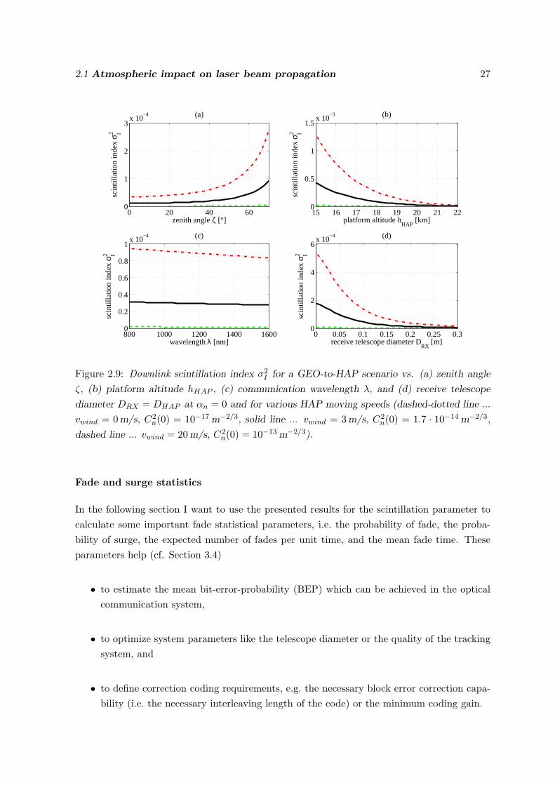
Because of diffraction, the cross section of the downlink laser beam will be much largerthan the diameter of the turbulent eddies in the atmosphere. Therefore, negligible beamwander, which would be caused mainly by large-scale turbulence near the transmitter, isexpected for the downlink. As shown in Fig.2.9(a) and (b), the scintillation index increaseswith increasing zenith angle ζ and decreasing platform altitude because the beam has to travelover a larger distance through the atmospheric layers. As in the uplink, the largest variationis found between 40 < ζ ≤ 70 and 15 km < hHAP ≤ 19 km. Figure 2.9(c) illustrates thewavelength dependence of the downlink scintillation index, showing the advantage of using alarge communication wavelength, especially in high turbulence conditions.
2The transverse correlation width for an uplink path is typically tens of meters or more.
2.1 Atmospheric impact on laser beam propagation 27
0 20 40 600
1
2
3x 10
−4
zenith angle ζ [°]
scin
tilla
tion
inde
x σI2
(a)
15 16 17 18 19 20 21 220
0.5
1
1.5x 10
−3
platform altitude hHAP
[km]
scin
tilla
tion
inde
x σI2
(b)
800 1000 1200 1400 16000
0.2
0.4
0.6
0.8
1x 10
−4
wavelength λ [nm]
scin
tilla
tion
inde
x σI2
(c)
0 0.05 0.1 0.15 0.2 0.25 0.30
2
4
6x 10
−4
receive telescope diameter DRX
[m]
scin
tilla
tion
inde
x σI2
(d)
Figure 2.9: Downlink scintillation index σ2I for a GEO-to-HAP scenario vs. (a) zenith angle
ζ, (b) platform altitude hHAP , (c) communication wavelength λ, and (d) receive telescope
diameter DRX = DHAP at αn = 0 and for various HAP moving speeds (dashed-dotted line ...
vwind = 0 m/s, C2n(0) = 10−17 m−2/3, solid line ... vwind = 3 m/s, C2
n(0) = 1.7 · 10−14 m−2/3,
dashed line ... vwind = 20 m/s, C2n(0) = 10−13 m−2/3).
Fade and surge statistics
In the following section I want to use the presented results for the scintillation parameter tocalculate some important fade statistical parameters, i.e. the probability of fade, the proba-bility of surge, the expected number of fades per unit time, and the mean fade time. Theseparameters help (cf. Section 3.4)
• to estimate the mean bit-error-probability (BEP) which can be achieved in the opticalcommunication system,
• to optimize system parameters like the telescope diameter or the quality of the trackingsystem, and
• to define correction coding requirements, e.g. the necessary block error correction capa-bility (i.e. the necessary interleaving length of the code) or the minimum coding gain.
28 CHAPTER 2. Channel model for optical links through the atmosphere
Probability of fade
The probability of fade, P (F > FT ), describes the probability that the loss (or fading depth),F , of the instantaneous received intensity, I, with respect to the received mean on-axis intensityis larger than a fade threshold FT . The term “on-axis” is defined as the line-of-sight (LOS)between the centers of the transmit and the receive telescope. The fade threshold parameterFT , in [dB], corresponds to the difference between the received on-axis mean intensity 〈I(0, L)〉after the transmission distance L and a smaller intensity threshold level IT , i.e.
FT = 10 log(〈I(0, L)〉
IT
). (2.17)
The probability of fade is deduced from mathematical models for the probability densityfunction (PDF), p(I), of the randomly fading irradiance signal [37, 51, 52, 53]. Assuming thatthe intensity fluctuation is an ergodic3 process, the probability of fade as a function of thethreshold level becomes the cumulative probability of the intensity, i.e.
P (F > FT ) = P (I < IT ) =∫ IT
0p(I)dI. (2.18)
In the weak fluctuation regime, the time-variant intensity of an optical wave can be describedby a lognormal PDF [54]
p(I) =1
I√
2πσ2I
exp
−[ln(
II(0,L)
)+ 2α2L2
W 2eff
+ 0.5σ2I
]2
2σ2I
, (2.19)
whereWeff (cf. eqn.(2.29)) is the effective beam radius at the receiver. In the strong fluctuationregime the gamma-gamma PDF
p(I) =2 (αpβp)
(αp+βp)/2
Γ(αp)Γ(βp)〈I(α,L)〉
(I
〈I(α,L)〉
)(αp+βp)/2−1
Kαp−βp
(2
√αpβpI
〈I(α,L)〉
), (2.20)
is a more accurate description [37]. Here Γ(x) =∫∞
0 e−ttx−1dt denotes the gamma function,whereas Kαp−βp(x) represents the modified Bessel function of the second kind and of orderαp − βp [37]. As an input, eqn.(2.20) requires the two parameters, αp and βp, which accountfor large-scale and small-scale intensity fluctuations and are given in [37]. For the case of anuplink, I derived new expressions for these parameters, which - different from the formulasgiven in [37] - take into account the pointing error and the effect of beam wander: Accordingto [51], the intensity, I, of the received optical wave can be modeled as a product I = xy,where x arises from large-scale turbulence and y from small-scale turbulence. If we assumethat x and y are statistically independent random processes, the second moment of intensityis
〈I2〉 = 〈x2〉〈y2〉 = (1 + σ2x)(1 + σ2
y), (2.21)
3For an ergodic process ensemble averages are equal to time averages.
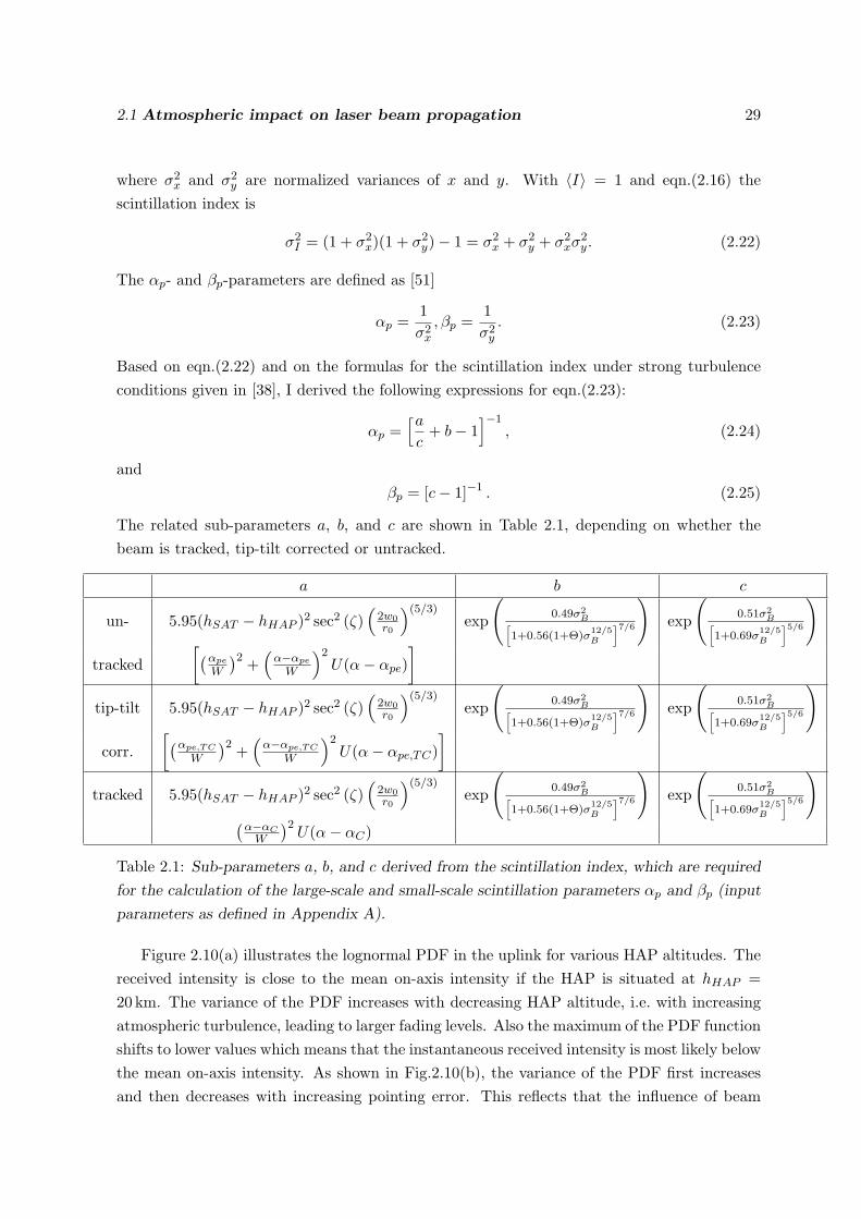
2.1 Atmospheric impact on laser beam propagation 29
where σ2x and σ2
y are normalized variances of x and y. With 〈I〉 = 1 and eqn.(2.16) thescintillation index is
σ2I = (1 + σ2
x)(1 + σ2y)− 1 = σ2
x + σ2y + σ2
xσ2y . (2.22)
The αp- and βp-parameters are defined as [51]
αp =1σ2x
, βp =1σ2y
. (2.23)
Based on eqn.(2.22) and on the formulas for the scintillation index under strong turbulenceconditions given in [38], I derived the following expressions for eqn.(2.23):
αp =[ac
+ b− 1]−1
, (2.24)
andβp = [c− 1]−1 . (2.25)
The related sub-parameters a, b, and c are shown in Table 2.1, depending on whether thebeam is tracked, tip-tilt corrected or untracked.
a b c
un- 5.95(hSAT − hHAP )2 sec2 (ζ)(
2w0r0
)(5/3)exp
(0.49σ2
B[1+0.56(1+Θ)σ
12/5B
]7/6
)exp
(0.51σ2
B[1+0.69σ
12/5B
]5/6
)tracked
[(αpe
W
)2 +(α−αpe
W
)2U(α− αpe)
]tip-tilt 5.95(hSAT − hHAP )2 sec2 (ζ)
(2w0r0
)(5/3)exp
(0.49σ2
B[1+0.56(1+Θ)σ
12/5B
]7/6
)exp
(0.51σ2
B[1+0.69σ
12/5B
]5/6
)corr.
[(αpe,TC
W
)2 +(α−αpe,TC
W
)2U(α− αpe,TC)
]tracked 5.95(hSAT − hHAP )2 sec2 (ζ)
(2w0r0
)(5/3)exp
(0.49σ2
B[1+0.56(1+Θ)σ
12/5B
]7/6
)exp
(0.51σ2
B[1+0.69σ
12/5B
]5/6
)(α−αCW
)2U(α− αC)
Table 2.1: Sub-parameters a, b, and c derived from the scintillation index, which are required
for the calculation of the large-scale and small-scale scintillation parameters αp and βp (input
parameters as defined in Appendix A).
Figure 2.10(a) illustrates the lognormal PDF in the uplink for various HAP altitudes. Thereceived intensity is close to the mean on-axis intensity if the HAP is situated at hHAP =20 km. The variance of the PDF increases with decreasing HAP altitude, i.e. with increasingatmospheric turbulence, leading to larger fading levels. Also the maximum of the PDF functionshifts to lower values which means that the instantaneous received intensity is most likely belowthe mean on-axis intensity. As shown in Fig.2.10(b), the variance of the PDF first increasesand then decreases with increasing pointing error. This reflects that the influence of beam

30 CHAPTER 2. Channel model for optical links through the atmosphere
0.1 0.2 0.3 0.4 0.5 0.6 0.7 0.8 0.9 1 1.10
0.1
0.2
0.3
0.4
0.5
0.6
0.7
0.8
0.9
1
normalized intensity I
norm
aliz
ed P
DF
αn=0
αn=0.2
αn=0.4
αn=0.6
αn=0.8
αn=1
0.2 0.4 0.6 0.8 1 1.2 1.4 1.6 1.8 20
0.1
0.2
0.3
0.4
0.5
0.6
0.7
0.8
0.9
1
normalized intensity I
norm
aliz
ed P
DF
hHAP = 1 km
hHAP = 5 km
hHAP = 10 km
hHAP = 15 km
hHAP = 20 km
(a) (b)
Figure 2.10: Normalized lognormal probability density function of the intensity for an un-
tracked uplink beam: (a) for varying HAP altitudes hHAP (αn = 0), (b) for different normal-
ized pointing errors αn = α/θeff (hHAP = 20 km).
wander is more severe if the (point) receiver is situated at the slope of the Gaussian beamthan at its peak or at its tail.
Figure 2.11 shows the probability for a fading larger than 1 dB as a function of the HAPaltitude in the uplink in different turbulence conditions. Below a height of h = 14 km, anuntracked beam clearly leads to a higher probability of fade than a tip-tilt corrected beam ora tracked beam. The often used standard Rytov model [54] approximates the tip-tilt correctedcase very well. At typical HAP altitudes - between 17 km and 22 km - the effect of beamwander becomes more and more negligible; the probability of fade for an untracked beam, atip-tilt corrected beam, and a tracked beam become virtually equal.
Probability of surge
The term surge denotes the event when the currently received intensity rises above the (tempo-ral) mean of the received intensity [55]. The probability of surge, P (S ≥ ST ), describes theprobability that the surge (or excess), S, of the instantaneous received intensity with respectto the received mean on-axis intensity after a link distance L is larger than the surge thresholdST . The surge threshold parameter, ST in [dB], giving the difference between the receivedon-axis mean intensity 〈I(0, L)〉 at α = 0 and a higher intensity threshold level IT , is definedas
ST = −10 log(〈I(0, L)〉
IT
). (2.26)
Following the approach for the probability of fade one can write the expression for the proba-bility of surge as
P (S ≥ ST ) = P (I ≥ IT ) =∫ ∞IT
p(I)dI = 1−∫ IT
0p(I)dI. (2.27)

2.1 Atmospheric impact on laser beam propagation 31
0 5 10 15 200
0.1
0.2
0.3
0.4
0.5
HAP altitude hHAP
[km]
prob
abili
ty o
f fad
e P
(F>
1 dB
)
(a) untracked beam
0 5 10 15 200
0.1
0.2
0.3
0.4
0.5
HAP altitude hHAP
[km]
prob
abili
ty o
f fad
e P
(F>
1 dB
)
(b) tracked beam
0 5 10 15 200
0.1
0.2
0.3
0.4
0.5
HAP altitude hHAP
[km]
prob
abili
ty o
f fad
e P
(F>
1 dB
)
(c) tip−tilt corr. beam
0 5 10 15 200
0.1
0.2
0.3
0.4
0.5
HAP altitude hHAP
[km]
prob
abili
ty o
f fad
e P
(F>
1 dB
)
(d) Rytov model
Figure 2.11: Uplink probability of a fading larger than 1 dB vs. HAP altitude for (a) an un-
tracked beam, (b) a tracked beam, (c) a tip-tilt corrected beam, and (d) when using the stan-
dard Rytov model for calculation (dashed-dotted line ... vwind = 0 m/s, C2n(0) = 10−17 m−2/3,
solid line ... vwind = 3 m/s, C2n(0) = 1.7 · 10−14 m−2/3, dashed line ... vwind = 20 m/s,
C2n(0) = 10−13 m−2/3).
Temporal statistical parameters
Temporal statistical parameters are, e.g., the expected number of fades per second orthe mean fade time. The number of fades per second gives the mean number of crossingsper second of the received intensity I below a specific threshold value IT , i.e. the mean numberof fades per unit time with a certain fading depth FT . The mean fade time in [s] representsthe average time at which the signal stays below a defined threshold FT . It depends on theprobability of fade as well as on the expected average number of fades per unit time.
When calculating temporal statistics, I treat the turbulent eddies as frozen in space whichmove across the observation path with an rms wind speed4
vt,RMS =
[1
50 · 103 − hHAP
∫ 50·103
hHAP
vt(h)2dh
]1/2
cos (ζ). (2.28)
4This assumption and the formula are in good accordance with the Taylor frozen turbulence hypothesis as
described in reference [37].

32 CHAPTER 2. Channel model for optical links through the atmosphere
fade level F [dB]Tfade level F [dB]T
fade level F [dB]T
0 5 10
10-5
100
fade level F [dB]T
pro
bab
ilit
y o
f fa
de
P(F
>F
T)
(a) probability of fade
0 0.5 110
-200
10-100
100
surge level S [dB]Tpro
bab
ilit
y o
f su
rge
P(S
>S
T)
(b) probability of surge an=a/q
eff
00.10.20.30.40.50.60.70.80.91
0 5 10
100
fade level F [dB]T
num
ber
of
fades
per
sec
ond
(c) number of fades, vHAP = 0 km/min
0 5 10
10-2
100
102
mea
n f
ade
tim
e [s
](d) mean fade time, vHAP =0 km/min
an=a/qeff
00.10.20.30.40.50.60.70.80.91
0 5 10
100
num
ber
of
fades
per
sec
ond
(e) number of fades, vHAP =11 km/min
0 5 1010
-4
10-2
100
mea
n f
ade
tim
e [s
]
(f) mean fade time, vHAP =11 km/min
00.10.20.30.40.50.60.70.80.91
an=a/q
eff
10-3
103
10-3
103
Figure 2.12: Uplink fade statistical parameters: (a) probability of fade, (b) probability of
surge, (c) expected number of fades per second for a HAP, (d) mean fade time for a HAP, (e)
expected number of fades per second for a UAV with vHAP = 11 km/min, (f) mean fade time
for a UAV with vHAP = 11 km/min.
For this formula, I changed the integration interval and the associated normalization of theBufton wind model (given in [37]) so that it ranges from the altitude of the HAP up to the

2.1 Atmospheric impact on laser beam propagation 33
mesosphere. The input parameter vt(h) takes into account the moving speed of the HAP andis calculated according to eqn.(2.12).
In Fig.2.12(a) I present the probability of fade in the uplink case as a function of thefading level FT for various normalized pointing errors αn. The probability of fade increaseswith increasing pointing error because it is calculated relative to the mean on-axis intensity,and because the Gaussian beam shape leads to higher scintillation at higher αn (cf. Fig.2.7).The probability of a surge - as shown in Fig.2.12(b) - is very small, especially for large pointingerrors. Figure 2.12(c) and (e) illustrate the expected number of fades per second as a functionof fading depth. At αn = 0.1 and a fading level of 0.1 dB, the number of fades per unittime is approximately 5 for a quasi-stationary HAP, but increases to 290 for a UAV movingwith vHAP = 11 km/min, because the turbulent atmospheric layers move faster in transversedirection to the laser beam. With increasing pointing error, a shift of the maximum numberof fades to higher fading levels is observed. This is because the instantaneous center of thebeam is no longer pointing at the center of the receiving telescope in the case of αn > 0,even if there is no turbulence. Because along the line-of-sight (LOS) between transmitter andreceiver (cf. Fig.1.3) the scintillation behavior is nearly identical, the maximum number offades decreases only slightly with increasing pointing error. The increase of the scintillationindex with increasing pointing error leads to a broadening of the curves as shown in Fig.2.12(c)and (e).
Figure 2.12(d) illustrates the increasing fade time with increasing pointing error. Forinstance, the mean fading time of a 2 dB fade is only 8 ms at αn = 0.3 but rises to 1 s atαn = 0.5. In order to compensate for burst errors by means of a forward-error correction (FEC)in combination with long data interleavers (as discussed in Section 3.4.6), a low pointing error istherefore of great importance because it reduces the length of burst errors. The required bursterror correction capability of an FEC is also reduced if the HAP moves faster (cf. Fig.2.12(d)and (f)) because fast moving atmospheric layers lead to short fadings - then only a smallnumber of consecutive data bits are disturbed.
Figure 2.13(a) shows the probability of fade in the downlink case. Although the scintillationindex is constant across the beam profile - so that off-axis and on-axis fluctuations are nearlyidentical - the pointing error still influences the probability of fade. This effect of a pointingerror on signal fading is mainly caused by the changes in the mean intensity due to the Gaussianbeam profile. It leads to an inherent loss of the received intensity at αn 6= 0 relative to themean received on-axis intensity in the case of αn = 0.
Unlike in the uplink case, the shape of the curves for the expected number of fades persecond are similar for all pointing errors (cf. Fig.2.13(c) and (e)), because the scintillationindex is invariant with respect to αn. The maximum expected number of fades per second fora HAP is approximately 31, with a mean duration of one single fade of 16 ms for zero pointingerror (cf. Fig.2.13(d)). The shift of the maximum number of fades to higher fading levels withincreasing pointing error is a consequence of normalizing the fading depth to the mean on-axis

34 CHAPTER 2. Channel model for optical links through the atmosphere
e f
Figure 2.13: Downlink fade statistical parameters for a point receiver: (a) probability of fade,
(b) probability of surge, (c) expected number of fades per second for a HAP, (d) mean fade
time for a HAP, (e) expected number of fades per second for a UAV with vHAP = 11 km/min,
(f) mean fade time for a UAV with vHAP = 11 km/min.
intensity, i.e. to αn = 0. For a moving HAP with velocity vHAP = 11 km/min the number offades are significantly larger than for vHAP = 0 km/min - leading also to shorter fading times -

2.1 Atmospheric impact on laser beam propagation 35
because the turbulent atmospheric layers move faster in transverse direction to the laser beam.
2.1.3 Beam spread loss
Atmospheric turbulence causes beam spread (cf. Fig.2.14) beyond the diffraction limiteddivergence θDL, leading to an effective divergence angle, θeff , which causes a degradation ofthe mean received optical power by a factor (θeff/θDL)2. For the calculation of this, additional,beam spread loss abs in [dB], I compare the diffraction limited beam radius WDL (determinedby the transmit telescope) of a Gaussian beam [41] to the effective beam radius [37]
Weff = WDL
[1 +
(DTX
r0
)5/3]3/5
, (2.29)
of the same beam but in the presence of turbulence, leading to
abs = 20log10
(Weff
WDL
), (2.30)
andabs = 20 log10[1 + (DTX/r0)(5/3)](3/5). (2.31)
x
y
θDL θeff
ω0DTX
(a) transmitter
(b) near-field
(c) far-field
WDL
Weff
spot-sizewith turbulence
spot-sizewithoutturbulence
Figure 2.14: Intensity distribution of a propagating laser beam (solid lines...beam spread
due to diffraction , dashed lines...beam spread due to diffraction and turbulence) (a) at the
transmitter, (b) in the near field, and (c) in the far field. Broadening of the beam due to
turbulence leads to additional loss in power.
For downlink paths only high-altitude turbulence - which is weak and relatively far awayfrom the transmitting source - has an influence on beam broadening. It is found that in thedownlink - where turbulent eddies are small compared to the beam diameter - the effectivespot size, Weff , is essentially the same as the diffractive spot size, WDL, [54]. Hence, beam
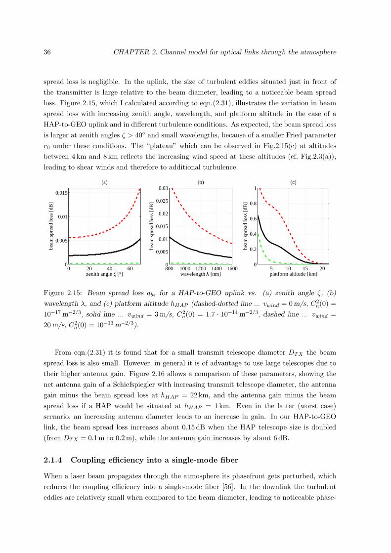
36 CHAPTER 2. Channel model for optical links through the atmosphere
spread loss is negligible. In the uplink, the size of turbulent eddies situated just in front ofthe transmitter is large relative to the beam diameter, leading to a noticeable beam spreadloss. Figure 2.15, which I calculated according to eqn.(2.31), illustrates the variation in beamspread loss with increasing zenith angle, wavelength, and platform altitude in the case of aHAP-to-GEO uplink and in different turbulence conditions. As expected, the beam spread lossis larger at zenith angles ζ > 40 and small wavelengths, because of a smaller Fried parameterr0 under these conditions. The “plateau” which can be observed in Fig.2.15(c) at altitudesbetween 4 km and 8 km reflects the increasing wind speed at these altitudes (cf. Fig.2.3(a)),leading to shear winds and therefore to additional turbulence.
0 20 40 600
0.005
0.01
0.015
zenith angle ζ [°]
beam
spr
ead
loss
[dB
]
(a)
800 1000 1200 1400 16000
0.005
0.01
0.015
0.02
0.025
0.03
wavelength λ [nm]
beam
spr
ead
loss
[dB
]
(b)
5 10 15 200
0.2
0.4
0.6
0.8
1
platform altitude [km]
beam
spr
ead
loss
[dB
]
(c)
Figure 2.15: Beam spread loss abs for a HAP-to-GEO uplink vs. (a) zenith angle ζ, (b)
wavelength λ, and (c) platform altitude hHAP (dashed-dotted line ... vwind = 0 m/s, C2n(0) =
10−17 m−2/3, solid line ... vwind = 3 m/s, C2n(0) = 1.7 · 10−14 m−2/3, dashed line ... vwind =
20 m/s, C2n(0) = 10−13 m−2/3).
From eqn.(2.31) it is found that for a small transmit telescope diameter DTX the beamspread loss is also small. However, in general it is of advantage to use large telescopes due totheir higher antenna gain. Figure 2.16 allows a comparison of these parameters, showing thenet antenna gain of a Schiefspiegler with increasing transmit telescope diameter, the antennagain minus the beam spread loss at hHAP = 22 km, and the antenna gain minus the beamspread loss if a HAP would be situated at hHAP = 1 km. Even in the latter (worst case)scenario, an increasing antenna diameter leads to an increase in gain. In our HAP-to-GEOlink, the beam spread loss increases about 0.15 dB when the HAP telescope size is doubled(from DTX = 0.1 m to 0.2 m), while the antenna gain increases by about 6 dB.
2.1.4 Coupling efficiency into a single-mode fiber
When a laser beam propagates through the atmosphere its phasefront gets perturbed, whichreduces the coupling efficiency into a single-mode fiber [56]. In the downlink the turbulenteddies are relatively small when compared to the beam diameter, leading to noticeable phase-

2.1 Atmospheric impact on laser beam propagation 37
front distortions within the receiving aperture (cf. Fig.2.17(b)). In the uplink the turbulenteddies are right in front of the transmitter and comparatively large relative to the opticalbeam. This leads to a large beam spread causing the phasefront disturbance to be negligiblewithin the small receiving aperture at the satellite (cf. Fig.2.17(c)).
In this Section I deal with the influence of a phase front disturbance in the downlink whencoupling into a single-mode fiber (SMF), e.g. when a single-mode coupled Erbium doped fiberamplifier (EDFA) is used as an optical preamplifier within the receiver. The Fresnel lossoccurring at the fiber’s input facet is not taken into account for these calculations. I calculatethe decrease in coupling efficiency assuming a perfectly aligned fiber relative to the couplinglens and a deterministic input field E with constant amplitude (cf. Fig.2.17(a)).
To describe the influence of the atmosphere on the phasefront of a propagating beam inthe downlink case I use the following formalism: The spatial phasefront disturbances after apropagation distance L can be described by the phase structure function [57]
Dϕ(ρd, L) = 〈(ϕ1 − ϕ2)2〉, (2.32)
where ϕ1 − ϕ2 denotes the phase difference at two points on the phase front separated by thedistance ρd. According to [40] the structure function for downlink channels can be modeledby
Dϕ(ρd, L) = 2.914k2ρ5/3d sec ζ
∫ hSAT
hHAP
C2n(h)dh, (2.33)
0.1 0.15 0.2 0.25 0.3105
106
107
108
109
110
111
112
113
114
115
telescope diameter DTX
[m]
gain
[dB
]
antenna gain [dB]antenna gain − beam spread loss [dB] at h
HAP=22 km
antenna gain − beam spread loss [dB] at hHAP
=1 km
Figure 2.16: Dependence of transmit antenna gain and beam spread loss on the transmit
antenna diameter DTX .

38 CHAPTER 2. Channel model for optical links through the atmosphere
apertureplane
focalplane
single-modefiber
circular pupil
a
2ρ
perturbedphasefront
wav
eguid
e
atmosphere
atmosphere
wav
eguid
e
(a) (c)(b)
Figure 2.17: (a) Coupling geometry: A thin lens focuses the incident field E, which is assumed
to have a constant amplitude but a statistically disturbed phase, onto the bare end of a single-
mode fiber. (b) Downlink: Negligible beam spread, large phasefront disturbance over receiving
aperture. (c) Uplink: Negligible phasefront disturbance, large beam spreading.
which, in combination with eqn.(2.15) for the Fried parameter r0, allows to calculate themean-square phase variation over an aperture of diameter D [47]
σ2ϕ = 1.0299
(D
r0
)5/3
. (2.34)
This formula confirms our interpretation of the Fried parameter r0 given in Section 2.1.2 asan aperture where the rms phase error is approximately 1 rad.
In the receiver, the optical input field E - which is collected by the receive telescope - isfocussed by a thin, diffraction limited lens to the bare end of a single-mode fiber, whose fielddistribution of the fundamental mode F0 is given by [14]
F0(r) ∝
J0(V
√1−B(r/ρ))
J0(V√
1−B)r ≤ ρ
K0(V√B(r/ρ))
K0(V√B)
r > ρ(2.35)
with ρ being the core radius of the single-mode fiber, J0 the Bessel function of the first kindand of zero order, K0 the modified Bessel function of the second kind and of zero order, V anormalized frequency, and B a normalized propagation constant. The coupling efficiency η isdefined as the ratio of the power carried by the fiber mode and the power available in the focalplane. It is possible - and often more convenient - to calculate the coupling efficiency in theaperture plane A [56], i.e. just in front of the coupling lens (cf. Fig.2.17). Then η is given by
η =∣∣∣∣∫∫
AEF ∗dA
∣∣∣∣2 (2.36)

2.1 Atmospheric impact on laser beam propagation 39
where E is the input field normalized to its overall power, and F ∗ is the conjugate complex ofthe field distribution of the fiber mode, backpropagated to the aperture plane A (cf. AppendixA.12):
F (r′) = F−1F0(r) =∫∫
AF0(r) exp [−j2π (νxx+ νyy)]dνxdνy
= H−1F0(r) = 2π∫ ∞
0F0(r)J0
(2π
r′
λfr
)rdr, (2.37)
where F−1 denotes the inverse Fourier transform and H−1 is the inverse Hankel transform.Inserting eqn.(2.35) into eqn.(2.37) yields
F (r′) = 2πρ2
λf
UJ1(U)J0(2π r′
λf ρ)− (2π r′
λf ρ)J0(U)J1(2π r′
λf ρ)
J0(U)(U2 −
(2π r′
λf ρ)2)
+
+ 2πρ2
λf
WK1(W )J0(2π r′
λf ρ)− (2π r′
λf ρ)K0(W )J1(2π r′
λf ρ)
K0(W )(W 2 +
(2π r′
λf ρ)2)
, (2.38)
with f being the focal length of the coupling lens, U = V√
1−B, and W = V√B. For a
fiber perfectly aligned relative to the coupling lens and for a deterministic input field E withconstant amplitude, η can be derived from eqn.(2.36) as
η =4χ2
(J2
1 (U)J2
0 (U)+K2
1 (U)K2
0 (U)
)·
·∣∣∣∣∫ χ
0
[UJ1(U)J0(r′)− r′J0(U)J1(r′)
J0(U) (U2 − r′2)+
+WK1(W )J0(r′)− r′K0(W )J1(r′)
K0(W ) (W 2 + r′2)
]exp
(jΦ(r′)
)r′dr′
∣∣∣∣2 , (2.39)
where χ is a design-parameter, which when optimized for maximum coupling efficiency atthe normalized single-mode cut-off frequency V = 2.405 equals χopt = 2.05 [56]. The phasefunction Φ(r′) covers any deviations from an ideal plane wavefront of the input field E. In thecase of a perfect phasefront, Φ(r′) = const., a maximum coupling efficiency of ηmax = 78.6%is achieved (cf. Fig.2.18(a) and [56]). To find the influence of a phasefront disturbance charac-terized by an rms value expressed in fractions of the wavelength λ, RMSλ, I model the phasefunction after a normal distribution with mean µϕ = 0 and standard deviation σϕ. Figure2.18(a) shows the coupling efficiency as a function of the rms phasefront perturbation in frac-tions of the wavelength. As expected, the characteristic is rather flat for small perturbations,but drops dramatically to very small values for large disturbances.
I have calculated the temporal mean value of the coupling efficiency into a SMF as afunction of the zenith angle for the following three scenarios (cf. Fig.2.18(b)): (i) a GEO-to-HAP link with the HAP at hHAP = 20 km and a receive telescope diameter of DRX = 0.135 m,

40 CHAPTER 2. Channel model for optical links through the atmosphere
(ii) a GEO-to-HAP link with DRX = 0.135 m and hHAP = 2400 m, and (iii) an GEO-to-groundlink withDRX = 1 m at the OGS. At high altitudes, η is roughly invariant with zenith angle andvery close to the maximum possible coupling efficiency of 78.6%. With decreasing height alsothe coupling efficiency decreases, due to increasing turbulence leading to noticeable phasefrontperturbations especially at zenith angles ζ > 50. If the diameter of the receive telescope islarge - like at the OGS - the phasefront perturbation over the aperture is very large, leadingto a poor coupling efficiency which in practice might well exclude the use of a single-modereceiver.
If the spatial period of the phasefront perturbation is clearly smaller than the pupil diam-eter, the normalized mean power coupling efficiency is often estimated by the Strehl ratio SR
[58]:η
ηmax= SR. (2.40)
The Strehl ratio is the ratio of peak power in the center of the image plane compared to thatof an equivalent unaberrated (diffraction-limited) system. It is useful to have an approximatepredictor for the coupling efficiency based on SR, which is also a standard indicator of theperformance of classical and adaptive (astronomical) imaging systems [59]. Under generalconditions, not limited to weak fluctuations, the Strehl ratio for an untracked beam can beapproximated by the expression [38]
SRuntr =[1 + (DRX/r0)5/3
]−6/5. (2.41)
Another widely used empirical formula is the Marechal approximation [59]
SRmar = exp [−σ2ϕ], (2.42)
where σ2ϕ is the variance of the phase aberration across the receiving aperture. An estimation
of the coupling efficiency using these approximations is shown in Fig.2.18(c), showing goodagreement with the computationally more intensive calculation of Fig.2.18(b).
The phase variance averaged over a circular aperture of diameter D as given in eqn.(2.34)drops to
σ2ϕ = 0.134
(D
r0
)5/3
(2.43)
if the tip and tilt components of the atmospheric perturbations are removed [47]. Thus applyingtip-tilt correction reduces the phase variance by a factor of 1.0299/0.134 = 7.7, independentof the diameter of the telescope. To account for active target tracking I incorporated eqn.(1.2)into the expression for the tilt-corrected Strehl ratio given in [38], leading to
SRtilt =
[1 +
(0.983− 0.856
1 + 0.007 (DRX/r0)5/3
)(DRX/r0)5/3
]−6/5
, (2.44)
which is in good accordance with the formulas given in [47] and with simulation results in[38, 58]. Figure 2.19 compares the coupling loss into a single-mode fiber for an untracked

2.1 Atmospheric impact on laser beam propagation 41
1 20 40 60 80 100 1200
0.2
0.4
0.6
0.8
1
coupli
ng e
ffic
iency
η
phasefront perturbation (λ/RMS )λ
(a)
0 20 40 60zenith angle °ζ [ ]
(ii)
(i)
(iii)
(i)
(ii)
(iii)0
0.2
0.4
0.6
0.8
1
coupli
ng e
ffic
iency
η
0
0.2
0.4
0.6
0.8
1
coupli
ng e
ffic
iency
η
(b) (c)
0 20 40 60
zenith angle °ζ [ ]
Figure 2.18: (a) Coupling efficiency η for a single-mode fiber as a function of the rms phasefront
perturbation RMSλ given in fractions of the wavelength λ. (b) Coupling efficiency and (c)
estimation of coupling efficiency using the Strehl ratio (dashed line...Andrews approximation,
eqn.(2.41), dashed-dotted line...Marechal approximation, eqn.(2.42)) vs. zenith angle for three
different link scenarios: (i) GEO-to-HAP with hHAP = 20 km and DRX = 0.135 m, (ii) GEO-
to-HAP with hHAP = 2400 m and DRX = 0.135 m, and (iii) GEO-to-OGS with hOGS = 2400 m
and DRX = 1 m.
beam (eqn.(2.41)) and for a tip-tilt corrected system (eqn.(2.44)) in a GEO-to-HAP downlink(for different turbulence conditions and using the parameters given in Table 1.2). The couplingloss shown here is normalized to the minimum coupling efficiency of 78.6%. When tracking isperformed by means of a tiltable mirror, the coupling loss is noticeable reduced.
From the results shown in Fig.2.18(c) and Fig.2.19 I conclude that using a telescope withD less than a few times r0 will, after tip-tilt correction, lead to a residual phase variance whichis small compared to unity and will therefore result in close-to-diffraction-limited performance.When comparing the results of Fig.2.19(a) to the diagrams shown in Fig.2.15, we observe thatthe beam spread loss in the uplink equals the coupling loss in the downlink. This is due tothe reciprocity of the optical communication link when the light is coupled into a single-modefiber, both at the terminal onboard the HAP and at the satellite.

42 CHAPTER 2. Channel model for optical links through the atmosphere
0 20 40 600
0.005
0.01
0.015
zenith angle ζ [°]
norm
aliz
ed c
oupl
ing
loss
[dB
]
0 20 40 600
0.5
1
1.5
2x 10
−3
zenith angle ζ [°]
norm
aliz
ed c
oupl
ing
loss
[dB
]
800 1000 1200 1400 16000
0.005
0.01
0.015
0.02
0.025
0.03
wavelength λ [nm]
norm
aliz
ed c
oupl
ing
loss
[dB
]
(a) untracked beam
800 1000 1200 1400 16000
0.002
0.004
0.006
0.008
0.01
wavelength λ [nm]
norm
aliz
ed c
oupl
ing
loss
[dB
]
(b) tip−tilt corrected beam
5 10 15 200
0.2
0.4
0.6
0.8
1
platform altitude [km]
norm
aliz
ed c
oupl
ing
loss
[dB
]
5 10 15 200
0.05
0.1
0.15
0.2
platform altitude [km]
norm
aliz
ed c
oupl
ing
loss
[dB
]
Figure 2.19: Normalized coupling loss into a single-mode fiber for a HAP-to-GEO downlink vs.
zenith angle ζ, wavelength λ, and platform altitude hHAP in the case of (a) an untracked beam
and (b) a tip-tilt corrected beam. (dashed-dotted line ... vwind = 0 m/s, C2n(0) = 10−17 m−2/3,
solid line ... vwind = 3 m/s, C2n(0) = 1.7 · 10−14 m−2/3, dashed line ... vwind = 20 m/s,
C2n(0) = 10−13 m−2/3).
2.1.5 Summary
The following statements summarize my results on the atmospheric impact on laser beampropagation in a HAP-GEO optical communication scenario:
• At the wavelength of 1550 nm there is a transmission window with a very low atmosphericattenuation of 0.22 dB at zenith (cf. Fig.(2.2)).
• Because the HAP is situated well above the clouds, changing weather conditions do notinfluence the communication link [4].
• As the impact of turbulence on the laser beam increases with increasing zenith angle,one should avoid communication links at zenith angles ζ > 50, where the atmosphericloss, the Fried parameter, and the scintillation index degrade significantly.
• Like in the downlink, where the effect of beam wander is negligible, beam wander ef-fects become negligible at HAP altitudes larger than approximately 14 km also in uplink

2.1 Atmospheric impact on laser beam propagation 43
communication scenarios (cf. Fig.(2.7)).
• Small fading depths can be achieved by keeping the pointing error small (cf. Fig.(2.12))and by using a large communication wavelength, such as 1550 nm, leading to a smallscintillation index (cf. Fig.(2.7)). Small fading depths allow for a smaller coding gainwhich reduces the complexity of error correcting codes.
• Short fading times can be achieved by keeping the pointing error small or by increasingthe HAP velocity (cf. Fig.(2.12) and Fig.(2.13)). A short fading time highly relaxes therequirements on the burst error correction capability of an FEC.
• With respect to fading it is of advantage to use small telescope diameters (cf. Fig.(2.8)).This results in a less severe influence of any pointing error. Of course one has to finda trade-off between low fading and high antenna gain. The transmit telescope diametercan be made larger the better the tracking scheme and the smaller the pointing error.
• Most fading-related parameters are strongly wavelength dependent. With decreasingwavelength the Fried parameter decreases, leading to an increasing scintillation indexand therefore to stronger fading. Because of the smaller beam divergence at lower wave-lengths, the impact of a pointing error on fading at, e.g., 850 nm is stronger than at1550 nm (cf. Fig.(2.7)).
• Although the scintillation index in the downlink is invariant with pointing errors α, theyare still detrimental for downlink channels because the mean intensity decreases in theradial direction according a Gaussian function (cf. Fig.(2.13)).
• The Strehl ratio - a standard indicator of the performance of classical imaging systems - isa good approximation for the coupling efficiency into a single-mode fiber (cf. Fig.(2.18)).
• While the phase perturbations in a downlink to an optical ground station may preventthe usage of a single mode EDFA in the receiver because of a low coupling efficiency, thephase aberrations are much smaller in typical GEO-to-HAP links, allowing for single-mode coupling if required (cf. Section(2.1.4)).
• Tip-tilt correction by means of a tiltable mirror to reduce phasefront abberations causedby the atmosphere is sufficient in order to achieve close-to-diffraction-limited perfor-mance. It greatly reduces the coupling loss into a SMF in the downlink as well as thebeam spread loss in the uplink (cf. Section(2.1.4)).

44 CHAPTER 2. Channel model for optical links through the atmosphere
2.2 Background radiation
In an optical communication link the receiver not only detects the signal from the transmitterbut also unwanted light from celestial bodies [13]. This may have a degrading effect on systemperformance. The spectral radiance5 of electromagnetic radiation at all wavelengths λ from aself-emitting source at temperature Tse is described by Planck´s law of black body radiation[60]:
R(λ, Tse) =2hc2
λ5
1exp (hc/λkTse)− 1
, (2.45)
where h and k are Planck’s and Boltzmann’s constant, and c is the speed of light. The majorsource of background radiation is the Sun. When the receiver is at the satellite sunlight isreflected from Earth; for a receiver at a HAP, a certain amount of background radiance hasto be expected from the sky due to scattered sunlight.
Principle
By employing the definition of the spectral radiance, the power spectral density in [W/m]accepted by the receiver’s telescope originating from a radiating body is
Nback(λ) = AeffD2RXπ
4L2R(λ), (2.46)
depending on DRX , the receive telescope diameter, L, the distance between the receiver andthe radiation source, and Aeff , the area of the source as seen from the receiver. It is importantto note that if the solid angle subtended by the source Ωs = D2
sπ/4L2 (where Ds is the diameter
of the radiation source) appears bigger than the receiver field of view (FOV) ΩFOV = πθ2FOV /4
the effective area is
Aeff =πθ2
FOV L2
4, (2.47)
where θFOV is the planar angle of the receiver’s FOV. For Ωs < ΩFOV the effective area isgiven as
Aeff =D2sπ
4. (2.48)
With the definitions of the number of spatial mode [61]
m =
ΩFOVΩDL
Ωs > ΩFOV
ΩsΩDL
Ωs < ΩFOV
(2.49)
with ΩDL = 4λ2/D2RXπ for the diffraction limited case, the power spectral density per fre-
quency unit in [W/Hz] becomes
Nback(f) = Nback(λ)λ2
c= m
λ4
cR(λ). (2.50)
5The spectral radiance is the unpolarized radiant power into an angle increment per unit area of source and
unit wavelength - given in [W / m3 sr] and commonly measured in [W / m2 nm sr].

2.2 Background radiation 45
2.2.1 Radiation from Earth
The radiation from Earth is caused by self emission as well as by reflected sunlight. Its spectralirradiance6 caused by these two effects can be calculated according to [62] as
Hrefl(λ) = R(λ, Tse,Sun)Ωs, (2.51)
andHself (λ) = (1−A)R(λ, Tse,Earth)Ωs, (2.52)
where the albedo A is the ratio of the amount of electromagnetic radiation reflected by theEarths surface to the amount incident upon it, Tse,Earth is its effective surface temperature forself emission, and Tse,Sun is the temperature of the sun.
With these formulas, eqn.(2.50) can be modified to express the background power spectraldensity as a function of the spectral irradiance:
Nback(f) = mλ4
cΩs
(Hself (λ)(1−A)
+Hrefl(λ)), (2.53)
where the spectral irradiance can be calculated with [61, 62, 26]
H(λ) = Hpeak(M,Teff )2.9 · 10−11m5K5
(λTeff )5 [exp (hc/λkTeff )− 1]. (2.54)
The maximum value of H(λ) concerning wavelength is denoted by [62]
Hpeak(M,Teff ) =3.1 · 10−9W/m210−M/2.5 max (R(λ, Teff ))∫ 0.61µm
0.51µm R(λ, Teff )dλ. (2.55)
It depends on the effective temperature, Teff , and on the magnitude, M , of the object. Thebrightness of an object relative to a reference star is called magnitude, with dimension 1. Forthe calculation of Hself (λ) this is the effective temperature of the Earth, while for Hrefl(λ) itis the temperature of the Sun.
Celestial body L [km] Ds [km] M Albedo Teff [K] Tse [K]
Sun 149.597 · 106 1.392 · 106 4.8 - 5900 -Earth 35786 12756.2 −22 0.22 5400 300
Table 2.2: Parameters for the calculation of power spectral density for the Earth (values taken
from [26, 34, 63, 64]).
The power spectral density Nback(f) caused by background radiation from Earth as afunction of the wavelength for a diffraction limited receive telescope with diameter DRX =0.135 m is shown in Fig.2.20. It is calculated using the parameters from Table 2.2. At thewavelength of λ = 1550 nm it amounts to Nback(f) = 2.89 · 10−25 W/Hz. Both self emissionand reflectance are taken into account, which is the reason why the curve shows two humps.
6The spectral irradiance is the radiant power incident upon a surface per unit surface area and unit wave-
length - given in [W/m3] and commonly measured in [W/m2nm].

46 CHAPTER 2. Channel model for optical links through the atmosphere
0.1 1 10 10
−34
10−32
10−30
10−28
10−26
10−24
10−22
10−20
wavelength λ [µm]
spec
tral
bac
kgro
und
nois
e po
wer
den
sity
N
back
(f)
[W/H
z]
1.55
Figure 2.20: Background noise power spectral density Nback(f) of the Earth received by a
diffraction limited telescope.
2.2.2 Radiation from the atmosphere
An unavoidable source of background radiation in the downlink case is the spectral radi-ance caused by the atmosphere due to scattering of incident radiation and to emission byatmospheric particles as a result of absorption of incident radiation [60]. Since the Earth’satmosphere represents a source extending over the whole hemisphere, m = ΩFOV /ΩDL (cf.eqn.(2.49)) applies for a HAP, independent of the telescope size. Measured spectral radianceR(λ) at sea level as a function of the wavelength for clear sky in daytime conditions is givenin [34], Fig.6-6. During nighttime, sky radiance caused by zodiacal light, galactic light, andscattered starlight can be approximated by [26]
R(λ) = Rpeak(λ)2.9 · 10−11m5K5
(λTeff )5 [exp (hc/λkTeff )− 1], (2.56)
with Rpeak(λ) = 2.9 W/m3sr and Teff = 6170 K. A simple model presented in [65] assumesthat the intensity of the scattered radiation decreases with increasing height according to
Nback(f, h) = Nback(f, 0) exp(− h
hs
), (2.57)
with h being the height above ground, given in [km], and hs = 7 km. The resulting powerspectral densities as received from sea level and from a HAP at an altitude of 20 km at awavelength of 1550 nm are given in Table 2.3.

2.2 Background radiation 47
Atmosphere conditions Nback(f) [W/Hz] h [km]
Day time, clear sky 1.544 · 10−26 0Day time, clear sky 8.867 · 10−28 20
Day time, sunlit clouds 1.544 · 10−25 0
Night time, clear sky 3.566 · 10−33 0Night time, clear sky 2.048 · 10−34 20
Table 2.3: Power spectral density of background radiation caused by the atmosphere at λ =1550 nm.

48 CHAPTER 2. Channel model for optical links through the atmosphere

Chapter 3
Optical communication subsystem
“Im Verkehr mit der Erde hat die Verstandigung mittelsLichttelegraphie den Nachteil, unverlasslich zu sein, weil ihreAnwendbarkeit davon abhangt, dass die Gegenstation auf derErde wolkenfrei ist. ”
H. Potocnik, Austrian engineer, 1892-1929
In optical free-space links, the required technical setup can be divided into two basic sub-systems ([15], cf. Fig.3.1): The optical communication subsystem deals with all aspectsof the information transport itself. The selection of an appropriate modulation format, trans-mitter and receiver setup, where the properties are tailored to the communication channel, isimportant to achieve a satisfactory performance. Quantitative measures for the performanceare for example the bit error probability (BEP) and the power margin. Link budget calcula-tions, taking into account all possible losses which might occur in transmitter, channel, andreceiver, are used to evaluate the achievable power margin at a certain target BEP.
PAT systems are also an essential part for successfully establishing optical free-spacelinks. As their name suggests, they operate in three phases for setting up the link [26, 20]:
Pointing is done by directing the transmission laser towards the receiver, based on a-prioriknowledge of the transmitter and receiver positions. A rough estimate of this informationis calculated from the orbit parameters of the satellite. Pointing is performed either bymoving the whole telescope with a two-axis gimbal or by applying a coarse pointingmirror.
To compensate for the pointing error caused by the finite speed of light and the relativevelocity of the two terminals, a point-ahead angle is applied to direct the transmit beamto the location where the receive terminal will be after the propagation time.
Acquisition is the process when the exact position of the receiver is located and the transmitlaser has to be readjusted towards this new location. Two techniques are commonlyused. One is to place a beacon laser at the transmit satellite (or the HAP) and point ittowards the receive HAP (or satellite). Generally, one or more separate lasers, operatingat wavelengths differing from that of the communication laser are used to generate thebeacon. The PAT system has to find this beacon, which is usually done by movingthe beacon beam within an uncertainty area, while the other terminal also scans theuncertainty region using a detector with a narrow field-of-view. Another approach is
49

50 CHAPTER 3. Optical communication subsystem
to place a retro-reflector at the receiver. For detecting the receiver, the PAT systemscans with the transmit laser (or an additional beacon laser) over the uncertainty area.As soon as the laser hits the retro-reflector it gets reflected back to the PAT system.The system can detect this reflection and with it, the receiver. Then the tracking phasebegins.
Tracking assures that the transmit laser is kept targeted onto the receiver. Coarse tracking,which is performed first, is done by means of a control loop driving a coarse pointingmirror. A fine tracking loop controls the fine steering mirror (which should have abandwidth of ≥ 1 kHz to accommodate vibrations [26]). The tracking function measuresthe angular error between the direction of the incoming and outgoing beams (taking intoaccount also the point ahead angle), which serves as a feedback for the tracking mirrors.CCD-arrays, CMOS-arrays (active pixel sensors), or quadrant (avalanche) photo diodes(QPDs) can be employed as tracking sensors. Often CCDs are employed for coarsetracking and QPDs for fine tracking because the former offer a wider FOV and the latterare more accurate [26].
Nonideal tracking leads to a tracking error which can have a high impact on the linkattenuation and therefore has to be considered in the link budget calculations.
transmitter
TX data
receiver
RX data
duplexer fine pointing telescope
coarsepointing
aquisition &tracking sensor
trackingmirror
out
in
(a) (b)
optical output signaloptical input signalelectrical signalcontrol signal
Figure 3.1: Laser communication terminal structure consisting of (a) communication subsys-
tem and (b) pointing, acquisition, and tracking (PAT) system [20].
In the following sections I want to present a detailed assessment of the performance of theoptical communication subsystem:
• First I will address the impact that the use of various optical modulation formats hason the performance and complexity of the communication subsystem. To quantitatively

3.1 Optical modulation formats: Assessment of performance and complexity 51
assess the performance of an optical receiver, its sensitivity is an often used criterion. It isdefined as the minimum input power required to achieve a certain bit error ratio. Aftera general discussion about the principles and the associated transmitter and receiverstructures of each modulation format (as given in literature, e.g. [66]), I am going topresent calculated receiver sensitivities, where I tailored the underlying system model tothe envisaged GEO-to-HAP scenario. A simulation tool developed within our researchgroup (SimTool) [67, 68] as well as commercially available software (VPI TransmissionMaker) were used for the computations. In a concluding trade-off between sensitivityand system complexity I select the most promising modulation format for our scenario,which is return-to-zero (RZ) intensity modulation.
• In a subsequent section about the transmitter setup, I report in detail the measurements Iperformed with the aim to characterize a new and potentially important semiconductorlaser source at the wavelength of 1550 nm, namely a vertical-cavity surface-emittinglaser (VCSEL). I show that, even though VCSELs are commercially available only fora comparatively short time, they offer some advantages when compared to traditionaledge-emitters such as distributed feedback (DFB) lasers.
• For a comparison of the performance of two different direct-detection receivers, opticallypreamplified and APD-based receivers (without preamplification), I had to reprogramthe simulation tool SimTool. My modifications are explained in Section 3.3, where I alsopresent the minimum optical input power which is required in our scenario to achieve abit-error-ratio of 10−9.
• In the last subsection, I present detailed link budget calculations, which take into accountall possible losses that might occur in the transmitter, in the channel, and in the receiver.My computations show that the communication link can be closed at a data rate of1 Gbit/s. At 10 Gbit/s additional performance enhancement measures, such as the useof forward-error-correction (FEC), are necessary. I present mathematical expressions,which allow to quantitatively take into account the advantageous effect of FEC, as wellas the detrimental influence of power fluctuations caused by atmospheric turbulence.Using this models I show that error-free optical communication (i.e. a BEP = 10−9) ispossible with a certain probability.
3.1 Optical modulation formats: Assessment of performance
and complexity
If information is to be transmitted over an optical free space channel, several ways exist how toimprint the data onto the laser beam. We can modulate the amplitude, the phase (frequency),or the polarization of the optical signal [66]. The selection of an optimum modulation formatallows to efficiently transmit information in terms of signal-to-noise ratio, data rate, and BEP.

52 CHAPTER 3. Optical communication subsystem
One important decision in the design of a communication link is the choice of an appro-priate signalling alphabet. Encoding M bits into one symbol using 2M states of the transmitsignal (e.g. 2M amplitude levels for amplitude shift keying) reduces the symbol rate Rs toR/M , with R being the bit rate. This offers the advantage of reduced speed requirements forthe optoelectronic components. However, for the same average transmit power and a constantsignal space, the BEP can be shown to increase with M [66]. Thus, if optoelectronic compo-nents are available for operation at a bandwidth of the order of the data rate (which is thecase for the scenario in mind), the choice of M = 1 is optimum.
Multilevel coding schemes that use pulses shorter than the bit duration are more robustwith regard to background radiation. A prominent example for such a scheme is pulse positionmodulation (PPM) [69]. However, such modulation formats have the disadvantage that a highexcess electrical bandwidth is needed to encode and decode the pulses with timing accuracyon a sub-bit-duration scale. Therefore, they are presently only competitive at low data rates(R < 1 Gbit/s).
In the following sections I discuss the impact of three different modulation techniques -intensity modulation, phase modulation, and polarization modulation - on the performance andcomplexity of the communication subsystem. A short description of the principle transmitterand receiver structure is followed by calculations of the receiver sensitivity for the GEO-to-HAP scenario, which are compared to the theoretical quantum-limited performance that canbe achieved with each modulation format. Finally, I present a trade-off between sensitivityand system complexity where I select the most promising modulation format for our scenario.
3.1.1 Intensity modulation
Two common modulation methods are used for amplitude modulation1 in today’s opticaltransmission systems, non-return-to-zero (NRZ) and return-to-zero (RZ) coding.
Principle
Non-return-to-zero on/off keying (NRZ OOK) is the simplest and most commonly used opticalintensity modulation (IM) format. By switching light on and off, the data is modulated ontothe optical carrier (cf. Fig. 3.2(a)). Here, the pulse duration Tp, i.e. the time where opticalpower is on, equals the bit duration Tb. The envelope of the pulse power in the time domain
1In communication engineering, the terms intensity modulation and amplitude modulation are often used as
synonyms, even though amplitude and intensity are not equal. The intensity is proportional to the square of
the amplitude (i.e. to the squared modulus of the complex amplitude of the electrical field).

3.1 Optical modulation formats: Assessment of performance and complexity 53
lasersource
externalmodulator
TX data
Transmitter
pulsecarver
frequency ff
op
tica
l p
ow
er
spec
tral
den
sity
f + Rf - R
10 d
B
time t
1/R
op
tica
l p
ow
er
c c c
10 d
B 1/R
frequency fo
pti
cal
po
wer
spec
tral
den
sity
time t
op
tica
l p
ow
er
f f + Rf - Rc c c
(a) NRZ (b) RZ
f=R for 50%RZf=R/2 for 33%RZ
Figure 3.2: Transmitter structure for intensity modulation, consisting of a laser source, an
external NRZ modulator, and an RZ pulse carver: (a) Optical spectrum and eye diagram of a
typical NRZ signal and (b) for an RZ signal (fc...center frequency, R...data rate) [66].
preamplifierEDFA
opticalbandpass
PIN photodiodemodule
decisionlogic
RX data
Receiver
electricallow-pass
Figure 3.3: Optically preamplified receiver structure for intensity modulation, consisting of an
optical preamplifier, an optical bandpass filter (fiber Bragg grating - FBG), a pin-photodiode,
a transimpedance amplifier, and an electrical low-pass.
may be approximated by [70]
|g1(t)|2 =
E12Tb
[1− sin
(παTb
(α2Tb − t
))], t ∈ [0, αTb]
E1Tb, t ∈ [αTb, Tb]
E12Tb
[1− sin
(παTb
(t−
(1 + α
2
)Tb))]
, t ∈ [Tb, (1 + α)Tb]
0, else
(3.1)
where E1 denotes the optical energy for a “1”-bit, α ∈ [0, 1] is the roll-off factor whichdetermines the rise and fall time of the envelope of the optical pulse power, and Tb is the bitduration.
Apart from its simplicity the advantage of NRZ is its bandwidth-efficiency (compareFig. 3.2(a) to Fig. 3.2(b)). The spacing of the spikes in the spectrum equals the data rate

54 CHAPTER 3. Optical communication subsystem
R. For ideal rectangular NRZ signals, all tones, except for the one at the center frequencyfc, would vanish. If the bandwidth at the transmitter and the receiver is limited, NRZ maysuffer from intersymbol-interference (ISI), leading to a small eye opening and a poor receiversensitivity.
Return-to-zero on/off keying (RZ OOK) is an impulsive coding modulation format. Itis usually generated out of a NRZ signal by means of a pulse carver [67]. This could beeither a sinusoidally driven electro-absorption modulator (EAM) or a Mach-Zehnder modulator(MZM). The pulse duration is specified by the duty cycle
DC =TpTb≤ 1. (3.2)
Typical values for the duty cycle of RZ pulses produced by a MZM are 33 % or 50 % [66, 68].For a mathematical description of the time domain signal it is necessary to replace Tb by Tp
in eqn.(3.1). For RZ, pulses are well separated in time. Therefore, the pattern effects fromlimited NRZ drive signal bandwidths are eliminated. The use of RZ yields in an improvedsensitivity of some 2 to 3 dB over NRZ [71]. This advantage comes at the expense of a broaderoptical spectrum (see Fig. 3.2a) and more complicated transmitter structures.
Theoretical work and experimental demonstrations [72, 73] aiming at a BEP of 10−9 haveshown optically preamplified receiver sensitivities down to 68 ppb for NRZ, approaching thequantum limit to within 2.2 dB, and 43 ppb for RZ, which is only 0.5 dB above the theoreticalquantum limit. The quantum limit of the optically preamplified receiver sensitivity taken asa reference here is 41 ppb. It is calculated assuming no polarization filtering, a chi-squareddistribution of the ASE noise after detection and a Gaussian distribution of the shot noise[74, 75].
Application of intensity modulation in HAP-to-satellite scenario
To calculate the BEP of a single-mode coupled receiver with optical preamplification (assketched in Fig.3.3) a simulation tool developed within our research group (SimTool) [67, 68]was used. Among the input parameters are the input pulse form, the background noise, theEDFA’s properties (noise figure and gain), the optical filter characteristics as well as band-width, conversion gain and noise of the diode module. Table 3.1 shows the used parameterswhich I tailored to the envisaged satellite-to-HAP scenario.
The calculated receiver sensitivities at a BEP of 10−9 for NRZ and RZ as a function of theoptical filter with bandwidth Bo, which was modeled as a fiber Bragg grating (FBG) bandpassfilter, are given in Fig.3.4. The electrical filter bandwidths (Be = 0.8R for NRZ and Be = 2.3Rfor RZ) were optimized to obtain maximum sensitivity. With NRZ, 74 ppb are required, whichis approximately 2.6 dB above the quantum limit. RZ coding with a duty cycle of 33% leadsto a sensitivity of 62 ppb at the optimum filter bandwidths, i.e. 1.8 dB above the quantumlimit. Depending on the optical bandwidth, a sensitivity gain of up to 2 dB can be achievedwhen using RZ instead of NRZ modulation because RZ coding is more tolerant with respect

3.1 Optical modulation formats: Assessment of performance and complexity 55
Parameter Value
Number of polarization modes 2
Extinction ratio of MZM ε = 20 dB
Preamplifier gain G = 39 dBPreamplifier noise figure F = 3.8 dB
Communication wavelength λ = 1550 nm
Detector sensitivity S = 0.8 A/WTransimpedance 1800ΩElectrical noise Nel = 10 pA/
√Hz
Dark current Id = 0.1 nA
Electrical filter fifth-order Bessel lowpassElectrical filter bandwidth optimized
Optical filter fiber Bragg gratingOptical filter bandwidth optimized
Background noise power density Nback = 8.867 · 10−28 W/Hz(clear sky, day, hHAP = 20 km)
RZ duty cycle 33%Pulse roll-off factor α = 0.4
PRBS length 27 − 1
Table 3.1: Parameters used for simulation of the receiver sensitivity of an optically preamplified
direct-detection (DD) receiver.
to suboptimum filtering (cf. Fig.3.4). This is especially important at data rates < 10 Gbit/s,where optimum optical filter bandwidths might not be technologically feasible. Dispersion freeFBG bandpass filters for example can be fabricated with bandwidths down to 0.15 nm [76],which at λ = 1550 nm corresponds to 18.7 GHz. At R = 1 Gbit/s this is much larger than theoptimum filter bandwidths of Bo = 1.8 GHz for NRZ and Bo = 3 GHz for RZ.
3.1.2 Phase modulation
Phase shift keyed (PSK) modulation formats carry the information in the optical phase. Indirect-detection (DD) receivers, the phase of the preceding bit can be used as a relative phasereference for demodulation. This has the advantage that no absolute phase-reference is re-quired. Such modulation format is denoted as differential phase shift keying (DPSK) [77].
Principle
Binary differential phase shift keying encodes information on a binary phase change betweenadjacent bits. A logical ‘1’ is encoded by a π phase change, whereas a logical ‘0’ is representedby the absence of a phase change. Like OOK, DPSK can be implemented in RZ and NRZ

56 CHAPTER 3. Optical communication subsystem
0 5 10 15 20 2560
70
80
90
100
110
120
optical filter bandwidth Bo [R]
NR
Z-O
OK
rec
eiver
sensi
tivit
y [
ppb]
(a)
0 5 10 15 20 25optical filter bandwidth Bo [R]
60
70
80
90
100
110
120
RZ
-OO
K r
ecei
ver
sensi
tivit
y [
ppb]
(b)
Figure 3.4: Optically preamplified direct-detection (DD) receiver sensitivity at a BEP of 10−9
vs. optical filter bandwidth (a) for NRZ-OOK and (b) for RZ-OOK as calculated with SimToolusing the parameters as given in Table 3.1 (ppb...photons per bit, R...data rate).
format. The main advantage from using DPSK instead of OOK comes from a maximum 3-dBsensitivity improvement at the receiver in an average power limited system [66, 77].
Phase modulation can either be achieved using an MZM, or by means of a dedicated phasemodulator (PM) (cf. Fig.3.5). An additional sinusoidally driven pulse carver may be used togenerate RZ-DPSK. The PM creates an optical signal with a constant envelope, but inevitablyintroduces chirp during the bit transitions of the modulated phase. Chirp is a parasitic fre-quency modulation, since the phase modulation in the PM does not occur instantaneously.Also any drive-waveform imperfections get directly mapped onto the optical phase [77]. In-stantaneous and perfect π phase jumps can be realized at the expense of some residual intensitymodulation by using a dual-drive MZM. Typical intensity and phase waveforms are shown inFig.3.5. The amplitude dips between two bits in the NRZ-DPSK eye represent the residualamplitude modulation of the MZM caused by finite NRZ drive signal bandwidth.
Since DPSK cannot directly be received with direct-detection techniques, a phase-to-amplitude converting element such as an optical delay interferometer (DI) has to be inserted inthe optical path at the receiver. Its differential delay is equal to the bit duration Tb. To exploitthe 3-dB sensitivity advantage of DPSK over OOK, a balanced receiver has to be employed[74], where the second output of the delay interferometer - yielding the inverted data pattern- is also made use of (cf. Fig.3.7(a)).
DPSK signalling theoretically performs best with preamplified DD receivers, yielding aquantum limit of 20 ppb at a BEP of 10−9 [74]. Sensitivities achieved experimentally areabout 2 to 3 dB above this value [77, 78].

3.1 Optical modulation formats: Assessment of performance and complexity 57
lasersource
phasemodulator
TX data
time t
1/R
time t
1/R
op
tica
l p
ow
er
time t
1/R
op
tica
l p
has
e
φ π0+
φ0
1
0
op
tica
l p
ow
er
1
0time t
1/R
op
tica
l p
has
e
φ π0+
φ0
precoder
lasersource
MZM
(a)
(b)
Figure 3.5: Schematic of a typical transmitter for phase modulation, consisting of a laser
source, (a) a phase modulator or (b) an MZM [77].
Application of phase modulation in HAP-to-satellite scenario
For the characterization of a single-mode coupled, optically preamplified balanced DPSK re-ceiver as it would be used within the envisaged HAP-to-satellite scenario, I employed a com-mercially available simulation tool (VPI Transmission Maker). It allows to fully take intoaccount the effects of intersymbol interference (ISI), as well as the exact probability densityfunction (PDF) of detection noise, which in the case of ASE caused by an optical preamplifieris a chi-square-like PDF [74]. This exact modeling is necessary because, as shown in [77], sim-ulation techniques based on a Gaussian noise assumption fail in predicting balanced receiverperformance. Figure 3.6 shows the calculated sensitivity in photons per bit (ppb) at a BEP of10−9 as a function of the optical filter bandwidth Bo. The electrical filter bandwidth Be wasoptimized to allow for maximum sensitivity. The optimum NRZ-DPSK receiver sensitivity (atBo = 1.8R) is 39 ppb, i.e. 2.9 dB above the theoretical quantum limit and 2.78 dB better thanNRZ-OOK (cf. Fig.3.4(a)).
As pointed out in [77] the sensitivity gain of advanced modulation formats like DPSK oftencomes at the price of increased system complexity. Imperfections in the used components thenlead to additional losses within the receiver. I therefore recalculated the penalties given in[77] for a nonideal NRZ-DPSK receiver using the parameter values given in Table 3.1. Figure3.7(a) illustrates the sensitivity penalty due to a coupling coefficient imbalance or a differencein the responsivity of the photodiodes in the balanced detector. For an amplitude imbalance
βimb =Su
Su + Sd, (3.3)
of βimb = 0.6, where Su is the responsivity of the photodiode in the upper branch and Sd
is the responsivity of the photodiode in the lower branch, the sensitivity penalty amountsto 0.25 dB. If one branch totaly fails (βimb = 1), i.e. for single-ended DPSK detection, the

58 CHAPTER 3. Optical communication subsystem
30
40
50
60
70
80
90
100
DP
SK
rec
eiver
sen
siti
vit
y [
ppb]
0 5 10 15 20 25optical bandwidth B [R]o
Figure 3.6: Optically preamplified NRZ-DPSK receiver sensitivity at a BEP of 10−9 vs. optical
filter bandwidth calculated with VPI Transmission Maker using the parameters as given in
Table 3.1 (ppb...photons per bit, R...data rate).
sensitivity penalty amounts to 2.8 dB, which is approximately the gain that NRZ-DPSK withbalanced detection can achieve over NRZ-OOK (cf. Fig.3.4(a) and Fig.3.6).
A phase imbalance - caused by a difference in the propagation delays between the outputports of the delay-interferometer (DI) and the combiner - leads to an additional loss in receiversensitivity (cf. Fig.3.7(b)). Such an imbalance can be either due to different path lengths ordue to differences in the electronic delays after detection. A 1-dB sensitivity penalty is to beexpected for a delay difference of a quarter of a bit duration.
Figure 3.7(c) shows the receiver sensitivity degradation for a mismatched interferometerdelay. A delay-to-data-rate mismatch of 10% leads to 0.4 dB extra sensitivity penalty.
The sensitivity penalty as a function of a phase difference
∆ϕ = 2π∆fTb, (3.4)
in the interferometer’s arms, i.e. an error in DI-phase tuning, is illustrated in Fig. 3.7(d). Itoccurs if there is an offset ∆f between the transmit laser frequency and the frequency leadingto perfect interference conditions in the DI, as set by the interferometer’s phase difference.
3.1.3 Polarization modulation
An alternative approach to intensity and phase modulation is to encode the digital data in thestate of polarization (SOP) of the launched light.

3.1 Optical modulation formats: Assessment of performance and complexity 59
0.6 0.7 0.8 0.9 1 1.1 1.2 1.3 1.40
2
4
Tb
delay to data rate mismatch [R·T ]b
(c)
0 2 4 6 8 10 12 14 16 18 200
0.5
1
1.5
DI phase imbalance [°]
Δφ
DP
SK
-NR
Z r
ecei
ver
sen
siti
vit
y p
enal
ty [
dB
]
(d)
DP
SK
-NR
Z r
ecei
ver
sen
siti
vit
y p
enal
ty [
dB
]
0 0.1 0.2 0.3 0.4 0.50
0.5
1
1.5
2
2.5
3
3.54
delay difference in detector branches [1/R]
(b)
DP
SK
-NR
Z r
ecei
ver
sen
siti
vit
y p
enal
ty [
dB
]
Tb
Δτ
0
1
2
3
DP
SK
-NR
Z r
ecei
ver
sen
siti
vit
y p
enal
ty [
dB
]
0.5 0.6 0.7 0.8 0.9amplitude imbalance
Tb
imbalance
(a)
Figure 3.7: Penalties in nonideal balanched NRZ-DPSK receiver due to (a) amplitude imbal-
ance, (b) delay imbalance, (c) delay-to-data rate mismatch in the delay interferometer, and
(d) DI phase imbalance. (Tb...bit duration, DI...delay-interferometer).
Principle
In a binary polarization shift keying (POLSK) system, a logical ‘1’ is associated with a givenstate of polarization (e.g. horizontal), while a ‘0’ is transmitted via the orthogonal polarizationstate (e.g. vertical). The main advantage over IM is a constant envelope of the optical signal,leading to a theoretically 3 dB better sensitivity in terms of peak power [74]. In an averagepower limited system, e.g. when using a booster EDFA, OOK and POLSK show equivalentperformance. While the state of polarization is altered due to birefringence when the lightpropagates within a standard single-mode fiber asking for active polarization management[79], the atmospheric channel preserves the SOP [34], allowing for the use of this modulationformat in the envisaged HAP-to-satellite scenario.
Various designs of polarization modulators have been proposed, mostly based on LiNbO3
devices to allow for high data rates [80, 81]. Interferometric type of devices - where a phasemodulator (PM) is used in one branch to introduce a desired phase shift - bear the problemof random phase drifts due to temperature fluctuations. Other modulators - based on induced

60 CHAPTER 3. Optical communication subsystem
birefringence - give a stable state of polarization but require high modulation voltage swings,not easy to allocate at high data rates.
preamplifierEDFA
opticalbandpass
decisionlogic
RX data
PBSPIN photodiode
module
electricallowpass
Figure 3.8: Schematic of a typical receiver for polarization modulation (PBS...polarization
beam splitter).
A schematic of a typical receiver for binary POLSK [82] is shown in Fig.3.8. An opticalfilter is placed at its input to reduce ASE and background noise. The optically preamplifiedsignal passes through a polarization beam splitter (PBS) which separates the two orthogonalpolarization states. These signals are subsequently detected by two photodiodes whose pho-tocurrents are combined with opposite sign. Since the input of the comparator is subject tothe noise of both receivers, the variance of the noise doubles in the decision element2. Theoutput of the comparator is connected to a decision element with decision threshold zero. Thisis an advantage over IM, which requires adaptive thresholding, reducing the complexity andincreasing the precision of the decision circuit in the POLSK receiver (cf. Fig.3.10).
Application of polarization modulation in HAP-to-satellite scenario
The quantum limited sensitivity of an optically preamplified balanced POLSK receiver at aBEP of 10−9 is 40 ppb [82, 74]. Figure 3.9 shows the calculated receiver sensitivity vs. theoptical bandwidth Bo for an optimized electrical filter bandwidth (Be = 0.75R), yielding aminimum number of 75 ppb for a BEP of 10−9, i.e. 2.7 dB above the quantum limit, whenusing the parameter values as given in Table 3.1. For the calculations I used the commerciallyavailable simulation tool (VPI Transmission Maker), which allows to take into account theeffects of ISI, as well as the exact probability density function (PDF) of detection noise.
As in the case of DPSK, imperfections in the receiver’s components might lead to anadditional sensitivity penalty. Figure 3.10(a) shows this penalty as a function of amplitudeimbalance (cf. eqn.(3.4)) in the branches of the balanced receiver, resulting from a couplingcoefficient imbalance or a difference in the responsivity of the photodiodes. The sensitivitypenalty is significantly smaller for adaptive tresholding (solid line) than for an absolute thresh-old (dashed line), because the amplitude imbalance in the two branches leads to a shift of theoptimum threshold to values unequal zero. A delay difference in the detector’s branches, due to
2A single-ended receiver compares a single, noisy signal with a deterministic threshold, while a balanced
receiver essentially compares two noisy signals with each other [77].

3.1 Optical modulation formats: Assessment of performance and complexity 61
0 5 10 15 20 2570
90
110
130
150
optical bandwidth B [R]o
PO
LS
K r
ecei
ver
sen
siti
vit
y [
pp
b]
Figure 3.9: Optically preamplified POLSK receiver sensitivity at a BEP of 10−9 vs. optical
filter bandwidth calculated with VPI Transmission Maker using the parameter values as given
in Table 3.1 (ppb...photons per bit, R...data rate).
different fibre lengths or due to differences in the electronic delays after detection, also leadsto a degradation of receiver sensitivity (cf. Fig.3.10(b)). A 1-dB penalty is to be expectedfor a delay difference of 0.3 times the bit duration Tb. At 10 Gbit/s, this corresponds to a6.1 mm (optical fiber) or 5.9 mm (coaxial cable) path length difference. Figure 3.10(c) and(d) illustrate the sensitivity penalty caused by imperfections of the polarization beam split-ter (PBS), due to a constant offset angle of the orthogonal polarization basis, and due to anon-orthogonality in the polarization basis. In the latter case, adaptive thresholding (dashed-dotted line) is of advantage when the logical “ones” are detected correctly and errors due toa non-orthogonal basis only occur during logical “zeros”, leading to a shift of the optimumthreshold to values larger than zero. The same statement holds true if the logical “zeros” aredetected correctly and errors due to a non-orthogonal basis only occur during logical “ones”. Ifthe non-orthogonal basis is placed such that errors occur equiprobable for both logical states,the sensitivity penalty is lower due to a wider eye opening, and there is no significant differ-ence whether adaptive thresholding (solid line) or absolute thresholding (dashed line) is usedbecause the optimum threshold is still zero (cf. Fig.3.10(d)).
3.1.4 Comparison of modulation formats
In Table 3.2 I compare the discussed modulation formats based on various assessment criteria,to make clear the advantages and disadvantages of each modulation technique.
System complexity and implementation risk is low for OOK formats. RZ just requires oneadditional pulse carver or some electronic pre-coding in comparison to NRZ (cf. Section 3.1.1).DPSK and POLSK require an additional demodulator module such as a phase-to-amplitude

62 CHAPTER 3. Optical communication subsystem
or a polarization-to-amplitude converting device and a balanced receiver setup (cf. Fig.3.5 andFig.3.8). This increases not only system complexity, but also penalties due to nonideal devicesand receiver setups, e.g. due to an unstabilized DI in the DPSK receiver or due to nonidealitiesin the polarization beam splitter within the POLSK receiver (cf. Fig.3.7 and Fig.3.10).
Equipment for setting up an OOK transmitter and receiver is available off-the-shelf, be-cause these modulation formats are applied nowadays in most terrestrial, fiber-based systems[31]. The devices have proven reliable and some are even already space-qualified or qualified formilitary purposes [83, 84, 85], which is necessary if the laser communication terminal (LCT) isput on a satellite. Devices for a setup using DPSK modulation are also commercially available.However, such systems have been primarily studied in the laboratory so far [86] and they stillhave to prove reliable in harsh environment. The same holds true for systems using binary
0.5 0.6 0.7 0.8 0.901
2
3
4
5
67
amplitude imbalance
PO
LS
K r
ecei
ver
sen
siti
vit
y p
enal
ty [
dB
]
imbalance
PBS
0 0.1 0.2 0.3 0.4 0.5delay difference in detector branches [1/R]
PO
LS
K r
ecei
ver
sen
siti
vit
y p
enal
ty [
dB
]
0 2 4 6 8 10 12 14 16 18 200
1
2
3
4
5
offset angle of POLSK demodulator [°]
PO
LS
K r
ecei
ver
sen
siti
vit
y p
enal
ty [
dB
]
0 5 10 15 20 25 300
1
2
3
4
5
non-orthogonality of demodulator [°]
adaptive threshold, ``ones´´ perfectly detectedabsolute threshold, perfectly detected``ones´´
adaptive threshold
absolute threshold
PO
LS
K r
ecei
ver
sen
siti
vit
y p
enal
ty [
dB
]
(d)
(a)
(c)
0
1
2
3
4
Δτ
PBS
(b)
PBS
γoff
`0´
`1´
PBSγorth
`0´
`1´
PBS
`0´
`1´
γorth2
γorth2
Figure 3.10: Penalties in nonideal POLSK receiver due to (a) amplitude imbalance βimb, (b)
delay imbalance ∆τ , (c) offset angle of the polarization basis in the POLSK demodulator γoff ,
and (d) non-orthogonal polarization basis γorth in the demodulator (R...data rate).

3.1 Optical modulation formats: Assessment of performance and complexity 63
Criteria OOK-NRZ OOK-RZ NRZ-DPSK NRZ-POLSK
System complexity low moderate high high
Development status + + ± −Costs low low moderate high
Theoret. receiver sensitivity @ BEP= 10−9 41 ppb 41 ppb 20 ppb 40 ppb(opt. preamp. RX, quantum limit)
Calculated receiver sensitivity @ BEP= 10−9 74 ppb 62 ppb 39 ppb 75 ppb(opt. preamp. RX, GEO-to-HAP scenario)
Table 3.2: Comparison of optical intensity modulation, phase modulation, and polarization
modulation formats (OOK...on/off keying, NRZ...non return to zero, RZ...return to zero,
DPSK...differential phase shift keying, POLSK...polarization shift keying, RX...receiver).
POSLK modulation, where some theoretical work was done [82] but experimental results arescarce.
Because of the lower technological maturity especially of POLSK systems and the highersystem complexity of DPSK when compared to OOK, the costs of implementing such systemsis expected to be much higher than when using intensity modulation.
Compared to OOK, POLSK theoretically offers a 3-dB sensitivity gain in terms of peakpower. For an average power limited system, e.g. when using a booster EDFA at the trans-mitter, OOK and POLSK show the same performance, whereas with DPSK one could gainsome additional 2.8 dB. Table 3.2 compares the quantum limited receiver sensitivities whenusing an optically preamplified DD receiver with no polarization filtering [74]. I also calculatedthe achievable receiver sensitivities for a GEO-to-HAP scenario, assuming parameters for thereceiver setup as given in Table 3.1. The noise sources which I took into account where thebackground noise from blue sky (day conditions), ASE noise (and all beat noise contributions)from the optical preamplifier, shot-noise from the photodetectors, and the noise of the elec-tronic circuitry. It is found that OOK-RZ approaches the quantum-limited sensitivity best,with a penalty as low as 1.8 dB. RZ coding is also much more tolerant to suboptimum filteringthan NRZ coded formats.
The turbulent atmosphere will influence all modulation formats in the same way (cf. Sec-tion 2.1). Beside a loss in power due to absorption and scattering there will be intensityfluctuations on a time scale large compared to the data rate, leading to fluctuations in theBEP. While OOK relies on the continuous optimization of the decision threshold, DPSK andPOLSK offer the advantage that the optimum threshold requires virtually no adjustmentsunder intensity fluctuations. Unlike in an optical fiber, the polarization information of theoptical signal will not be altered by the atmospheric channel [34]. Under the frozen atmo-sphere assumption (cf. Section 2.1.2), the atmospheric impact on the signal’s phase will notchange over two consecutive bit intervals. Therefore, phase perturbations will not influencethe phase-to-amplitude conversion when using DPSK modulation.

64 CHAPTER 3. Optical communication subsystem
In the previous sections it was found that the use of RZ coded signals allows to closelyapproach the quantum limited sensitivity, outperforming NRZ based systems by several deci-bels. RZ coding is also much more tolerant to suboptimum filtering than NRZ coded formats,which is especially of advantages at data rates around 1 Gbit/s where optimum optical filterbandwidths are not technologically feasible. Simultaneously, the complexity of OOK systemsis reduced when compared to DPSK or POLSK based systems. Therefore, I choose RZ-OOKas the appropriate modulation format for our GEO-to-HAP scenario.
3.2 Transmitter
3.2.1 Principle
The transmitter onboard the HAP or the GEO satellite has the task to imprint data ontothe optical carrier. The block diagram of a basic intensity modulation (IM) transmitter setup[66] is shown in Fig.3.11: A directly modulated laser module serves as a source with on-off-keying capability. In order to establish a sufficiently high extinction ratio (or to generate RZmodulated signals), an additional external Mach-Zehnder modulator (MZM) or an electro-absorption modulator (EAM) can be used. In our scenario, the wavelength of the laser isset to λ = 1550 nm (193.4 THz) (cf. Section 1.3), but in general any wavelength within theC-band (from 1530 nm to 1565 nm) can be used, which is the wavelength range where Erbium-doped fiber amplifiers (EDFAs) are available [33]. The modulated data signal is amplified bya booster EDFA to achieve an optical output power of up to 10 W.
Table 3.3 shows an assessment of the internal losses and the available power at the outputof the transmitter (i.e. at the output of the booster EDFA) for two different transmitterconcepts, one using a directly modulated laser, the other an external modulator. Because ofthe saturation of the booster EDFA, up to 40 dBm of average transmit power can be achievedat the output of the transmitter [32, 87], independent of the modulation technique.
lasercontroler
(precoded)data
lasermodule
MZMboosterEDFA
Figure 3.11: Block diagram of OOK transmitter.

3.2 Transmitter 65
Transmitter concept 1 Transmitter concept 2(directly modulated laser) (external modulation)
Gain [dB] Power at output [dBm] Gain [dB] Power at output [dBm]
Laser module - 0 - 0Optical connector −0.2 −0.2 −0.2 −0.2Optical connector - −0.2 −0.2 −0.4
MZM - −0.2 −3.5 −3.9Optical connector - −0.2 −0.2 −4.1Optical connector −0.2 −0.4 −0.2 −4.3
Booster EDFA saturated 40 saturated 40
Output power 40 40
Table 3.3: Typical power budget and loss within the transmitter.
Most devices incorporated in the transmitter have already been studied in great detail [31,33], as they are often used in traditional fiber-based communication systems. Yet, we recentlyreported on the use of a new and potentially important light source at the wavelength of1550 nm, namely a vertical-cavity surface-emitting laser (VCSEL) [88]. In the following section,I want to present the principle of this laser source, as well as the results of our measurementsconcerning the static and dynamic characteristics of such VCSELs. A comparison between“conventional” DFB-lasers and VCSELs is presented in Section 3.2.2.4, showing the benefitsand drawbacks of these laser sources, especially in the face of the envisaged HAP-to-satellitecommunication scenario. However, to allow for a comprehensive comparison between the twolaser sources, also parameters were measured which are not of particular importance for opticalcommunication from HAPs, e.g. chirp, which is only of interest for narrow optical filtering (i.e.at high data rates of 10 Gbit/s), or the spectral purity of the laser.
3.2.2 Vertical-cavity surface-emitting laser
Semiconductor laser sources based on InGaAs, such as distributed-feedback (DFB) or vertical-cavity surface-emitting lasers (VCSELs) may be used for OOK direct modulation at thewavelength of 1550 nm and at data rates up to 10 Gbit/s. Even if external modulators areused, such semiconductor laser sources may serve as continous-wave (CW) light sources.
While DFB lasers at 1550 nm are well established in laser communications [33, 31], VC-SELs operating at this wavelength are relatively new devices. Today, there are only twomanufacturers world-wide from which long-wavelength (i.e. C-band) VCSELs are commer-cially available, Vertilas (Germany) and RayCan (Korea). Therefore, I want to present theresults of a measurement, which were performed to thoroughly determine the static and dy-namic characteristics of (just recently) commercially available, long-wavelength VCSELs. Itis found that due to their low threshold current and power consumption they are potentially

66 CHAPTER 3. Optical communication subsystem
interesting transmitter sources for laser communication terminals (LCTs) onboard of HAPsor satellites. Laser modulation drivers with only small modulation swings would be requiredfor directly modulating the VCSEL, which is a great advantage at high transmission speeds.
A VCSEL (cf. Fig.3.12) principally consists of two distributed Bragg reflector (DBR) mir-rors, which are alternating layers of two semiconductor materials with different refractiveindices. Each layer has a thickness of a quarter of the laser wavelength in the material [33]. Inthe active area, the emitted radiation is amplified by stimulated emission and reflected by theDBRs, leading to laser oscillation [14]. For the fabrication of a 1550-nm VCSEL, InP-basedsemiconductor materials are used (e.g. InGaAsP/InP) [89].
The laser resonator is such that the laser light is emitted normal to the chip surface, i.e.the light is emitted vertically, which gives the device its name. Therefore, these lasers canbe tested directly on the wafer, leading to a cost advantage when compared to DFB (edge-emitting) lasers, which need to be cleaved out of the wafer prior to testing [33]. Another effect,due to the square shape of the laser waveguide, is the resulting perfect circularity of the outputbeam as opposed to the elliptical profile of a conventional DFB laser, reducing the couplingloss into a single-mode fiber [31].
light -
+
-
contact & heat sink
n-region
p-regionactive region
p+
n+n-region
upper DBR
isolation isolation
BTJ
n-region
Figure 3.12: Structure of VCSEL with buried tunnel junction (BTJ) [90].
For my work I experimentally investigated the properties of single-mode fiber pigtailed,uncooled VCSELs with buried tunnel junction (BTJ) [89, 91] at the wavelength of 1550 nm.The next sections discuss
• the static characteristics of commercially available VCSELs from the manufacturers Ver-tilas (Germany) and RayCan (Korea),
• the dynamic characteristics of these laser sources, and
• the differences between the properties of VCSELs and typical attributes of “traditional”DFB lasers.

3.2 Transmitter 67
3.2.2.1 Static characteristics of VCSELs
For the measurements of the static characteristics, four VCSELs from each manufacturer wereavailable. I am presenting the results for two VCSELs (one from Vertilas, one from RayCan)as typical examples, as all VCSELs showed very similar behaviour. Where necessary, I am alsogoing to discuss the sample variance based on measurements on the other available VCSELsources.
Figure 3.13(i) illustrates the output power, P , vs. drive current, I, characteristics and thelaser voltage, U , vs. laser current, I, characteristics measured at various ambient tempera-tures for a Vertilas VCSEL (Fig.3.13(a)) and a RayCan VCSEL (Fig.3.13(b)). The ambienttemperature was controlled by means of a temperature chamber, positioning the temperaturemeasuring head right next to the lasers. The laser voltage is relatively stable with temperature,revealing differential resistances
rd =∆u∆i
(3.5)
in the lasing region of rd ≈ 45Ω (Vertilas) and rd ≈ 104Ω (RayCan).The P-I curves show the laser threshold Ith, above which the laser starts to be operational,
i.e. where the optical output power increases significantly with increasing laser current. Figure3.13(ii) gives the temperature dependence of the lasers’ threshold current between 25C and50C, which in this temperature region is about 0.013 mA/K for the Vertilas VCSEL and0.04 mA/K for the RayCan device. Threshold currents of the Vertilas VCSEL vary betweenIth,min = 0.61 mA (at 25C) and Ith,max = 0.89 mA (at 50C), while the RayCan VCSELshows a much larger temperature dependence, with Ith changing from Ith,min = 1.6 mA (at25C) to Ith,max = 2.4 mA (at 50C). For DFB lasers, typical threshold currents would stillbe higher, between 10 mA and 20 mA [33, 14].
The maximum output power (achieved around 9 mA) dramatically drops with increasingtemperature; the power decreases about 40% (from P = 1.25 mW to P = 0.75 mW) between25C and 50C for the Vertilas VCSEL and about 50% (from P = 0.56 mW to P = 0.28 mW)for the RayCan VCSEL. We attribute a part of this power drop to an increasing coupling lossinto the single-mode pigtail, as the beam shape changes, i.e. the divergence angle increases,with increasing temperature [90]. Compared to a DFB laser [33, 68], the VCSELs offer a loweroptical output power by a factor of 5, which is of no concern if a booster EDFA is used (cf.Table 3.3). However, the large variation of the P-I curves with temperature might require anadaptive control of the operating point when directly modulating the lasers, and a temperaturestabilized environment within the LCT.
The P-I characteristics of both VCSELs are approximately linear between the thresholdcurrent and a laser current of 6 mA (cf. Figure 3.13(i)). The slope efficiency
ηsl =∆p∆i
(3.6)
is the mean value of the incremental change in optical power P for an incremental changein forward current I when the device is operating in the lasing region of the P-I curve. My

68 CHAPTER 3. Optical communication subsystem
measurements revealed slope efficiencies from 0.178 W/A (at 25C) to 0.122 W/A (at 50C)and from 0.106 W/A (at 25C) to 0.07 W/A (at 50C) for the Vertilas and the RayCan VCSEL,respectively. These values are similar to DFB lasers, where slope efficiencies between 0.12 and0.2 W/A at room temperature are reported [92, 31].
(b)
(i)
0
0.2
0.4
0.6
0.8
1
1.2
laser current I [mA]0 1 2 3 4 5 6 7 8 9
0
0.2
0.4
0.6
0.8
1
1.2
25 C°30 C°40 C°50 C°
25 30 35 40 45 500.6
0.7
0.8
0.9 (ii)
(a)
laser current I [mA]0 1 2 3 4 5 6 7 8 9
0
0.1
0.2
0.3
0.4
0.6
op
tica
l p
ow
er[m
W]
P
0.5
0
0.4
0.8
1.2
1.6
2
2.4
lase
r v
olt
age
U [
V]
25 C°30 C°40 C°50 C°
25 30 35 40 45 50ambient temperature [°C]
thre
sho
ld c
urr
ent
I[m
A]
th
2.3
2.2
2.1
2
1.9
1.8
1.7
1.6
2.4 (ii)(i)
ambient temperature [°C]
lase
r v
olt
age
U [
V]
thre
sho
ld c
urr
ent
I[m
A]
th
op
tica
l p
ow
er[m
W]
P
Ith
Ith
Figure 3.13: Measured static characteristics at various temperatures of (a) a Vertilas VCSEL
and (b) a RayCan VCSEL: (i) P-I and U-I characteristics, (ii) threshold current vs. tempera-
ture.
Long-wavelength VCSELs usually operate in a single longitudinal mode due to the shortresonator length, d, (of typically 2 to 5µm) [90], which leads to a mode spacing [14] ∆f ≈c/(2dn) (where n is the group refractive index of the laser material) approximately equalor even larger than the gain bandwidth. In Fig.3.14(i), I show the wavelength spectra of aVertilas VCSEL (cf. Fig.3.14(a)) and a RayCan VCSEL (cf. Fig.3.14(b)) at 30C at a lasercurrent of 3 mA, revealing a second spectral peak which is offset by some 0.35 to 0.6 nm. Thismeasurement was performed using an optical spectrum analyzer (OSA), with a resolutionbandwidth of 0.01 nm. The side-mode suppression ratio, which is defined as the ratio ofmain longitudinal mode power to side longitudinal mode power, is at least 33 dB. Laserswith side-mode suppression ratio larger than 30 dB are considered as single mode [31]. Themeasured center wavelengths are not exactly at the nominal channel wavelength of 1550 nm,deviating by 1.85 nm (Vertilas) and 13.2 nm (RayCan). Such deviations were observed for

3.2 Transmitter 69
all of the eight purchased VCSELs. We therefore conclude that the production process forlong-wavelength VCSELs can not perfectly be controlled yet to fabricate these lasers at anexact target wavelength. That the emission wavelength of the VCSELs is not constant acrossthe wafer and that therefore some sample variance has to be expected was also confirmed bypersonal communication with the manufacturer and in literature [93].
Figure 3.14(ii) gives the center wavelength λ of the VCSELs as a function of the lasercurrent, I, for various ambient temperatures. The emission wavelength of the Vertilas VC-SEL increases with I at a slope of approximately 0.45 nm/mA (for the RayCan VCSEL it is0.49 nm/mA). The temperature dependence of the wavelength was 0.12 nm/K (0.13 nm/K forRayCan). At temperatures between 25C and 50C, all Vertilas VCSELs emitted within a±3 nm wavelength range around 1550 nm. A selection process might reduce this deviation,however, a temperature stabilized environment onboard the HAP or the satellite when us-ing VCSELs is required anyway to compensate for the temperature dependence of the centerwavelength.
1547
1548
1549
1550
1551
1552
1547.9 1548.1 1548.3 1548.5 1548.7-80
-60
-40
-20
0
wavelength [nm]λ
op
tica
l p
ow
er P
[dB
m] I = 3 mAbias
(i)
1536.4 1537 1537.6-80
-60
-40
-20
0
op
tica
l p
ow
er P
[dB
m]
wavelength [nm]λ
I = 3 mAbias(i)
1 2 3 4 5 6 7 8 9 101535
1536
1537
1538
1539
1540
1541
1542
1543
1544
laser current I [mA]
wav
elen
gth
nm
λ[
]
25 C°30 C°40 C°50 C°
1 2 3 4 5 6 7 8 9 10laser current I [mA]
wav
elen
gth
nm
λ[
]
25 C°30 C°40 C°50 C°
(ii)
(ii)
(a)
(b)
Figure 3.14: (i) Unmodulated VCSEL spectra at 30C and I = 3 mA and (ii) center wavelength
vs. laser current at various ambient temperatures for (a) a Vertilas VCSEL and (b) a RayCan
VCSEL. (Optical power, P , measured within the resolution bandwidth of the OSA which
equals 0.01 nm.)
3.2.2.2 Dynamic characteristics of VCSELs
The experimental characterization of the dynamic behaviour of the VCSELs is necessary ifthey are considered for direct modulation. For the measurements, we mounted the pigtailed

70 CHAPTER 3. Optical communication subsystem
0
-10
-20E
/O c
on
ver
sio
n c
har
acte
rist
ic [
dB
]0 1 2 3 4 5 6 7 8 9 10
frequency [GHz]0 2 4 6 8 10 12
-20
-18
-16
-14
-12
-10
-8
-6
-4
-2
02
frequency [GHz]
E/O
co
nv
ersi
on
ch
arac
teri
stic
[d
B]
-5
-15
(a) (b)
2.5 Gbit/s 10 Gbit/s 10 Gbit/s 1 Gbit/s 2.5 Gbit/s 10 Gbit/s
RC element
VertilasVCSEL
50Ω line
RCelement
50Ω line
RayCanVCSEL
Figure 3.15: Small-signal modulation characteristics and eye diagrams for (a) Vertilas VCSEL
(dashed line...electrical characteristics improved by RC element) and (b) RayCan VCSEL.
TO-46 laser packages at the end of a 50Ω-microstrip line, with an SMA connector on the otherend for electrical connection (cf. insets of Fig.3.15). Such careful laser mounting significantlyflattened the VCSELs modulation response across the data bandwidth.
For the measurement of the small-signal modulation characteristic, a vector network ana-lyzer (VNA) was used to directly modulate the lasers with an electrical power level of −10 dBm,which was chosen low enough to avoid nonlinear behaviour. As a detector we applied an In-GaAs pin-photodiode with a bandwidth of 55 GHz and a specified ripple in the frequencydomain smaller than ±0.3 dB. Figure 3.15 shows the results for two VCSELs at 25C, wherethe curves are normalized to the maximum value. The modulation responses drop below −3 dBat frequencies between 3 and 4 GHz, which is in accordance with the specifications given bythe manufacturers (as the VCSELs were rated for 2.5 Gbit/s modulation). However, we wereable to operate the Vertilas VCSELs at data rates of up to 10.7 Gbit/s. As shown below, thiswas made possible by mounting the VCSELs at the end of a 50Ω-microstrip line, in series withan RC element consisting of a 1 pF capacitor parallel to a resistor (cf. Fig.3.16(c)). The RCelement significantly improved the VCSELs’ modulation response at frequencies larger 3 GHz(cf. Fig.3.15(a), dashed line), which was originally limited mainly by the package. The high-frequency behaviour of the RayCan VCSELs could not be improved, because it was mostlydetermined by the intrinsic properties of the laser chips themselves. The dimensioning of theRC element worked as follows: Figure 3.16(a) shows the equivalent RF-schematic of the laserincluding the main electrical parasitic elements. The inductance Lwire which we approximatedwith 1 nH was caused by a 1 mm (visible) wire from the case to the microstrip line. Beside thesmall intrinsic capacitance of the VCSEL [94], CV CSEL ≈ 0.5 pF, the differential resistance

3.2 Transmitter 71
Rd = 45 Ω of the laser (taken from the P-I curve measurements in Fig.3.13(a)), and the rel-ative large inductance Lbond ≈ 2 nH of the 2 mm bonding wire3, the capacitance of the caseCcase ≈ 10 pF [94] was the main reason for bandwidth limitation. To compensate the influence
R45Ω
d
(a) VCSEL's RF schematic
C0.5pF
VCSELC10pF
case
L2nH
bondL1nH
wire50Ω
L1nH
wire
R182Ω
(c) 1550 nm VCSELinclusive RC element
C11pF
50Ω
TO-46
Rd
(b) frequency compensatedvoltage splitter
Ccase
C1pF
1
50Ω
TO-46
R1
TO-46
Figure 3.16: (a) RF-schematic of 1550 nm VCSEL including parasitic elements, (b) principle
of frequency compensated voltage splitter, (c) optimal RC element for the 1550 nm VCSEL.
of Ccase, the principle of a frequency compensated voltage splitter (Fig. 3.16(b)) was used.The time constant of τ1 = R1 ·C1 had to be equal to the time constant of τV CSEL = Rd ·Ccase.A second requirement for rise and fall times of at most 50 ps for non problematic 10 Gb/s op-eration is a small capacitance C1. This is because of the resulting RC low pass filter consistingof the 50 Ω source resistance from the microstrip line and the input capacitance of the wholeschematic. This means that the time constant τsource = Rsource · C1 must be in the range of50 ps, leading to
C1 =τsourceRsource
=50 ps50 Ω
= 1 pF and (3.7)
R1 =Rd · Ccase
C1=
45 Ω · 1 pF1 pF
= 45 Ω. (3.8)
Figure 3.16(c) shows the final circuit for this 1550-nm VCSEL. Lastly, the overall frequencyresponse was experimentally optimized and thus the value of R1 changed to 82Ω, because ofthe additional influence of other parasitic elements.
The improvement due to the modifications of the RF circuitry is clearly observed in the eyediagrams of the Vertilas VCSEL given in Fig.3.15(a), which shows a much wider eye opening(at the data rate of R = 10 Gbit/s) in the case that the RC element is included.
Another important indicator for the quality of the modulation is the extinction ratio
ζex = 10 log(P1
P0
), (3.9)
which we defined for the measured NRZ eye diagrams as the ratio of the average optical powerP1 during a logical “one” to the average optical power P0 during a logical “zero”. The maximumachievable extinction ratios ranged from approximately 20 dB at 1 Gbit/s to 10 dB at 10 Gbit/s
3We had to cut open one of the VCSEL packages to investigate the electrical mounting of the lasers.

72 CHAPTER 3. Optical communication subsystem
(cf. Table 3.4), which is comparable to extinction ratios provided by directly modulated DFBlasers [68, 66] or even electro-absorption modulators (EAMs) (cf. EAM datasheet, AppendixC.3). But the extinction ratio also depends on the driving conditions. At high bias currentand low modulation swings, i.e. when the laser drive current for a logical ‘0’ is much largerthan the threshold current, the achieved extinction ratio at 10 Gbit/s was only 4 to 5 dB.
When driving the VCSELs with a pseudorandom bit sequence (PRBS) of length 231 − 1using NRZ modulation and measuring the (back-to-back) bit error ratio (BER) as a functionof the average optical power, we observed that the lasers yield better results when drivenwith low data signal amplitudes. When using large modulation swings, the ‘0’-level comesclose to the lasing threshold, resulting in better extinction ratios at the expense of significantamplitude overshoots and increased BER. Figure 3.17 shows the measured BER using a stan-dard 10-Gbit/s pin-type photoreceiver (cf. Appendix C.4) in combination with an optimumelectrical lowpass filter at optimized driving conditions. The hatched area marks the samplevariance of the VCSELs. For our measurements four VCSELs from each manufacturer wereavailable. We found no indication of an error floor, neither for the Vertilas VCSELs (measuredat R = 10 Gbit/s) nor for the RayCan VCSELs (measured at R = 1 Gbit/s due to bandwidthlimitations of the lasers). The measurements for the RayCan VCSELs were also repeated us-ing an APD-based receiver, leading to a sensitivity gain of approximately 7.8 dB. The dashedlines in Fig.3.17 represent reference measurements using a DFB laser in combination with anEAM. It can be observed that the use of a directly modulated VCSEL and an EAM resultsin virtually the same performance at R = 1 Gbit/s (where the achieved extinction ratios withboth techniques were similar). At R = 10 Gbit/s we have some 3.9 dB penalty when using theVCSELs, because of a ∼ 5 dB better extinction of the external modulator.
Table 3.4 summarizes the most important dynamic characteristics of the VCSELs undertest, which are the minimum rise and fall time (measured between 10% and 90% of the max-imum amplitude), the 3-dB bandwidth, and the maximum achievable extinction ratios atvarious data rates.
Parameter Symbol Remarks Vertilas Vertilas VCSEL RayCanVCSEL with RC-element VCSEL
Min. rise time tR 10% to 90% 168 ps 32 ps 68 psMin. fall time tF 10% to 90% 118 ps 50 ps 123 ps
3-dB bandwidth B 3.2 GHz 10.9 GHz 3.7 GHz
Achievable at R = 10 Gbit/s - 9.9 dB -extinction ζex at R = 2.5 Gbit/s 13.6 dB 15 dB 14.6 dB
ratio at R = 1 Gbit/s 15 dB 22 dB 20 dB
Table 3.4: Measured dynamic characteristics of commercial available long-wavelength VCSELs.

3.2 Transmitter 73
R = 1 Gbit/sI = 4.5 mA
I = 4.8 mAbias
mod (p-p)
-25 -20 -15 -1010
-910
-8
10-7
10-6
10-5
10-4
10-3
10-2
10-1
average optical power P [dBm]
bit
err
or
rati
o B
ER
(a)
-40 -36 -32 -28 -24 -20average optical power P [dBm]
10-9
10-8
10-7
10-6
10-5
10-4
10-3
10-2
10-1
bit
err
or
rati
o B
ER
(b)
APD gain
APD-RX pin-RX
pin-RX
R = 10 Gbit/sI = 4.5 mA
I = 6.6 mAbias
mod (p-p)
Figure 3.17: Measured BER vs. average optical power for (a) Vertilas VCSELs at R =10 Gbit/s using a pin-receiver (solid line) and (b) RayCan VCSELs at R = 1 Gbit/s (solid
lines) using either a pin or an APD receiver. The dashed lines mark reference measurements
performed with a DFB laser in combination with an EAM using a PRBS pattern length of
231 − 1. Hatched areas mark the sample variance. (R...data rate, Ibias...laser bias current,
Imod...peak-to-peak modulation current)
3.2.2.3 Characterization of frequency chirp in VCSELs
Direct modulation of semiconductor lasers introduces a parasitic frequency modulation (i.e. achirp) to the optical signal, which broadens the spectrum by a factor of approximately
√1 + α2
c
[67, 95, 31], where αc is usually denoted as chirp parameter or linewidth enhancement factor.In VCSELs, chirp results from refractive index changes associated with changes of the carrierdensity, which leads to this time dependence of the instantaneous frequency.
Here I report on the measurement of the (bit pattern dependent) phase dynamics of adirectly data-modulated 1550-nm VCSEL from Vertilas at the data rate of R = 10 Gbit/s[96]. Based on these measurements I calculate the linewidth enhancement factor αc andthe frequency chirp for different driving conditions and modulation patterns. In contrast toearlier measurements [97], which only quantify the chirp-parameter for sinusoidal modulationat certain output powers, the results presented here perfectly describe the behaviour of theVCSEL under operating conditions typically for data transmission. The linear approximationof the chirp parameter as a small-signal parameter depends highly on the driving conditionsof the laser, thus our complete dynamic characterization leads to a better understanding ofthe properties of the device.
The time-resolved intensity and phase of the output of the VCSEL are obtained by per-forming phase retrieval on the measured sonogram
S(τ,Ω) =∣∣∣∣∫ ∞−∞
E(ω)G(ω − Ω)e−jωτdω∣∣∣∣2 (3.10)

74 CHAPTER 3. Optical communication subsystem
of the output [98], where E(ω) corresponds to the Fourier transform of the optical field E(t).When the VCSEL is driven by a periodic pattern, the sonogram of the output can be obtainedby measuring the intensity of the filtered output after filtering by a (tunable) spectral filterG(ω) with, e.g., a sampling oscilloscope for various central frequencies of the filter. Thesonogram can therefore be seen as a measure of the time of arrival of a series of spectral slices.
patterngenerator EAM
phaseshifter
FPetalon
OSA
computer(LABVIEW)
pattern
clock
10Gbit/s
VCSEL
τ Ω
temporalgating
spectralfiltering
S( , )τ Ω
complex amplitudeof pulse and filter
E( ) and G( )ω ω
spectral filtering E( ) G( - )ω ω Ω
Fourier transform òωτ
ωE( ) G( - )e d-j
ω ω Ω∞
-∞
ò ω ω Ω ωωτ
E( ) G( - )e d-j
-∞
∞ 2intensity
(a) (b)
Figure 3.18: (a) Setup for the acquisition of a sonogram (EAM...electro absorption modulator,
FP...Fabry Perot, OSA...optical spectrum analyzer). (b) Procedure for generating a sonogram
[98].
Figure 3.18(a) shows the principle measurement setup used for the acquisition of a sonogramS(τ,Ω). The VCSEL under test is directly modulated with a bit pattern repeatedly generatedby the pattern generator at a data rate of 10 Gbit/s. Temporal gating of the signal is per-formed by means of an electro absorption modulator (EAM), which is driven by a clock signalsynchronized with the periodic signal under test. The relative delay τ between the pulsesand the gate is modified with a computer-controlled phase shifter. The sonogram is thencomposed of the spectra of the gated pulse train, measured with a tunable Fabry-Perot (FP)etalon (0.02 nm bandwidth), where the center frequency offset of the filter, Ω, from the centerfrequency of the pulses is also adjusted via the computer. The optical spectrum is measuredwith an optical spectrum analyzer (OSA) which transmits this information to the computer tocalculate S(τ,Ω). Applied in reverse, this process, which is depicted in Fig.3.18(b), is the basisfor the component generalized projection algorithm [99, 98] (implemented with the softwareLABVIEW [100]), which is used to perform phase retrieval. This leads to the field emittedby the laser
E(t) = A(t) exp (−jω0t+ jφ(t) + jφ0) (3.11)
without any assumption. In eqn.(3.11), A(t) is the time dependent envelope of the opticalfield, ω0 is the carrier frequency, φ(t) is the time dependent phase, and φ0 is a constant.
The linewidth enhancement factor αc of a laser is defined as the change in the real part ofthe refractive index as a function of the change in carrier numbers divided by the differentialgain [95]. In a modulated VCSEL, the presence of large data signals leads to a phase shiftduring the transitions of the data (transient chirp) as well as to a long-term shift in the laser

3.2 Transmitter 75
frequency (adiabatic chirp). An expression for the frequency chirp in terms of optical outputpower P (t) is [101, 33]
∆f(t) =αc4π
(d
dtlnP (t) + κP (t)
), (3.12)
where κ is a constant depending on the geometry of the laser, the Planck’s constant and theoptical frequency. In eqn.(3.12) the first term represent the transient chirp, whereas the secondterm determines the adiabatic chirp. In the transient chirp limited regions, such as the risingand falling edges, αc can be calculated according to [102]
αc = −2P (t)dφ/dt
dP/dt. (3.13)
3
4
5
6
7
8
9
10
3
4
5
6
7
8
9
10
0 200 400 600 800time [ps]
inte
nsi
ty [
a.u.]
phas
e [r
ad]0 1 0 1 0 1 0 0 1 0 1 0 1 0
(a)
I =2.4mA
I =3.2mA(p-p)bias
mod αc = 4.73
4
5
6
7
8
9
10in
tensi
ty [
a.u.]
3
4
5
6
7
8
9
10
phas
e [r
ad]
0 200 400 600 800time [ps]
I =4.5mA
I =6.6mA(p-p)bias
mod αc = 5.4
(b)
Figure 3.19: Intensity (solid line) and phase response (dashed line) of the VCSEL modulated
with a “0101010” pattern at a data rate of 10 Gbit/s with (a) bias current Ibias = 2.4 mA and
modulation swing Imod = 3.2 mA and (b) Ibias = 4.5 mA and modulation swing Imod = 6.6 mA.
Figure 3.19 shows the measurement results for two different driving conditions using a NRZ“010101”-pattern at a data rate of 10 Gbit/s as modulation signal. A bias current of Ibias =2.4 mA and a modulation swing of Imod = 3.2 mA lead to a linewidth enhancement factor ofαc = 4.7. For a larger bias current of Ibias = 4.5 mA and modulation swing of Imod = 6.6 mAthe chirp parameter increases to a value of αc = 5.4. The measurement shows that αc of theVCSEL depends on the driving conditions and has its minimum values at low optical outputpowers, i.e. for low bias currents. This is as expected, because the larger the bias current andmodulation swing, the larger the change in carrier density, which leads to larger variations inthe refractive index and thus to more chirp, as shown below.
The chirp parameter is only a simplified description [103], whereas the used measurementtechnique allows a complete characterization of the device by measuring the intensity and phaseof the output without assuming functional pulse shapes. Figure 3.20 shows the intensity (solidlines) and phase (dashed lines) response of the VCSEL using different modulation patterns,

76 CHAPTER 3. Optical communication subsystem
for two different driving conditions. From the derivation of the phase response, I calculatedthe frequency chirp ∆f (i.e. the frequency difference between ‘0’ and ‘1’). The measured chirpis higher for low bias currents and modulation swings, e.g. the chirp for Ibias = 2.4 mA andImod = 3.2 mA is approximately 10 GHz higher than for Ibias = 4.5 mA and Imod = 6.6 mA.For patterns with a low number of zeros the extinction ratio is small, leading to a lower amountof chirp ∆f . The measurement of the intensity shows that the turn-on behaviour is improvedif the ”zero”-level of the modulation signal I0 is further above the threshold level Ith. For anincreasing I0/Ith, the overshoot decreases significantly (cf. Fig.3.20(a) and (b)), also stronglyaffecting the chirp characteristic in this region.
2
4
6
8
10
0 200 400 600 800time [ps]
0 0 1 0 0 0 0 0
2
4
6
8
10
inte
nsi
ty [
a.u
.]
ph
ase
[rad
]
0 0 1 1 0 0 0 0 0 1 1 1 1 1 1 1 0 1 1 1 0 1 1 1
0
2
4
6
8
10
ph
ase
[rad
]0 0 1 0 0 0 0 0 0 0 1 1 0 0 0 0 0 1 1 1 1 1 1 1 0 1 1 1 0 1 1 1
0
2
4
6
8
10
inte
nsi
ty [
a.u
.]
I =2.4mA
I =3.2mAbias
mod (p-p)
(a)
(b)
I =4.5mA
I =6.6mAbias
mod (p-p)
Δf=12.5 GHz
Δf=22 GHz Δf=13.5 GHz
Δf=13 GHz
Δf=21.5 GHz Δf=13 GHz
Δf=11 GHzΔf=11 GHz0 200 400 600 800
time [ps]0 200 400 600 800
time [ps]0 200 400 600 800
time [ps]
Figure 3.20: Pattern dependence of the intensity (solid lines) and phase (dashed lines) response
including the measured chirp in GHz (∆f is the frequency drift between a logical ‘0’ and a ‘1’)
for (a) bias current Ibias = 2.4 mA and modulation swing Imod = 3.2 mA and (b) Ibias = 4.5 mA
and modulation swing Imod = 6.6 mA.
3.2.2.4 Comparison between DFB-laser and VCSEL
In this section I briefly discuss the differences between distributed feedback (DFB) lasers,which are widely used in optical communication systems at 1550 nm, and the relatively newlong-wavelength VCSELs. I base this comparison on information given in standard literatureon optical communications [31, 33, 14], as well as on own measurements which I performedfor this thesis and during previous projects [68, 92, 88, 96]. The benefits and drawbacks ofVCSELs in comparison to DFB lasers are as follows:
- When compared to DFB lasers for telecommunication purposes, VCSELs have a lower opticaloutput power by a factor of typically 5 to 10 [31, 33, 14]. However, in the envisaged HAP-to-satellite link, several Watts (rather than mW) of optical output power are required.

3.2 Transmitter 77
Thus an optical booster amplifier has to be implemented within the transmitter anyway.In this case, VCSEL output powers around 1 mW are sufficient.
- In our experiments the temperature dependence of the the optical output power was verylarge. When increasing the temperature from 25C to 50C, the power dropped by some40% for the Vertilas VCSEL and by 50% for the RayCan VCSEL. For DFB lasers, smallerpower drops of approximately 15% to 21% over this temperature range are reported[31, 104]. In the case of the VCSELs, we attribute a part of the decrease in output powerto a decreasing coupling efficiency into the single-mode pigtail, because the divergenceangle of the output beam also increases with temperature [90]. However, the use of agood temperature control system onboard the HAP or the satellite is inevitable, be it tostabilize the optical output power, wavelength, or operating point of the laser source.
- Our measurements showed that the commercially available VCSELs have a strong samplevariance in center wavelength. The Vertilas VCSELs had emission wavelengths whichwere off by (maximum) ±3 nm from the target wavelength of 1550 nm. This is attributedto difficulties in the fabrication process, leading to variations in emission frequenciesacross the wafer. Precise compositional control is difficult to achieve over an entire waferduring growth of many quaternary layers required for the DBR mirrors, because thecomposition is quite temperature dependent [93]. For DFB lasers, a typical wavelengthuniformity of ±1 nm across the wafer was reported [105].
For an implementation into a laser terminal, a selection process could be performed be-forehand, selecting VCSELs which emit at the required target wavelength. However, incase of a HAP-to-satellite communication scenario, the absolute value of the emissionwavelength is not as important as, e.g., in fiber-based dense wavelength division multi-plexing (DWDM) systems, where channel wavelengths have to be closely matched to themultiplexer passbands standardized by the ITU.
- Regarding space qualification, not much official information could be obtained. This canbe explained by the fact that the driving market for 1550-nm components is terrestrialfibre-optic communication. However, some customized, space and radiation qualifiedDFB laser devices, e.g. from Modulight [106, 84], are available. A study stating thatthreshold currents and optical output powers of InGaAsP-based lasers fabricated for1550 nm are only affected minimally by irradiation, is published in [107]. For long-wavelength VCSELs space qualification testing still has to be accomplished.
∼ In our experiments the temperature dependence of the threshold current was such that forthe Vertilas VCSEL Ith increased by approximately 46% and for the RayCan VCSELit increased by 50% when going from 25C to 50C. For DFB lasers, the temperaturedependence of the threshold current is given as [14, 31]
Ith ∝ exp(T
T0
), (3.14)

78 CHAPTER 3. Optical communication subsystem
where T is the absolute temperature, and T0 is a constant which is approximately 60 Kfor InGaAsP based lasers. When increasing the temperature from 25C to 50C, thiswould correspond to an increase of Ith by some 52%, which is very similar to the VCSELresults.
∼ The optical output power of VCSELs is low, but also the required laser current is verysmall, leading to good slope efficiencies (e.g. 0.178 W/A for the Vertilas VCSEL), whichare comparable to the slope efficiencies of commercially available DFB lasers [92, 31].
∼ The measured side mode suppression ratio of the VCSELs was always larger than 33 dB,which is on the lower side of DFB lasers, for which typical values of 30 to 50 dB arereported [31]. Lasers with such large side mode suppression ratios, i.e. ≥ 30 dB, areconsidered as longitudinally single-mode [31].
∼ DFB lasers and VCSELs show similar chirp behaviour, with αc (the linewidth enhancementfactor) beeing in the range between 2 and 5, depending on the driving conditions. Thismay lead to an up to 0.8 dB penalty in receiver sensitivity (cf. Section 3.3.2.1), becausethe optical spectrum is broadened by a factor of approximately
√1 + α2
c [31].
∼ Commercially available VCSELs can be modulated up to 10 Gbit/s. Using an RC-elementto slightly modify the electrical properties of the package, we were able to achieve 3-dB bandwidths of up to 11 GHz with the Vertilas VCSELs. While a data rate of R =10 Gbit/s is typical for DFB laser applications [31], direct modulation of DFB lasers wasalso reported up to R = 40 Gbit/s [108]. However, as shown in Section 3.4, the maximumdata rate for which the HAP-to-satellite link can be closed is 10 Gbit/s.
∼ The temperature dependence of the emission wavelength in VCSELs is comparable to thatof an DFB laser [31], i.e. in the range of 0.1 to 0.13 nm/K. Over a 20 K change, theemission wavelength in a VCSEL will vary by less than 2.6 nm.
+ An often cited advantage of VCSELs is their potentially low cost [33]. The laser light isemitted normal to the wafer surface, allowing for on-chip testing and high volume massproduction.
+ The circular output aperture of a VCSEL in combination with a proper cavity design leadsto a single transverse output mode with a circular Gaussian shape (and low divergenceangle). This greatly reduces the complexity and cost of coupling optics (compared toedge-emitters like DFB lasers) and increases the coupling efficiency into the fiber [109].Coupling efficiencies of up to 90% can be achieved with VCSELs [31, 109], due to thegood overlap of the fundamental mode of the VCSEL and the optical field in the fibercore. For DFB lasers, the coupling efficiency is typically 40 to 50% because of theirelliptical spot size [31, 90].

3.2 Transmitter 79
+ VCSELs have a much lower power consumption than DFB lasers due to their small thresh-old and laser currents (cf. Fig.3.13). This eases the design of modulation drivers at hightransmission speeds, because only small modulation swings are required.
+ My measurements showed that excellent extinction ratios (up to 10 dB at R = 10 Gbit/s)can be obtained when modulating the VCSEL. Achievable extinction ratios and BERsare therefore only a little bit worse than when using a DFB module with integratedEAM.
In summary, my investigations on long-wavelength VCSELs have shown that these lasers arepotentially interesting light sources for the application onboard HAPs or satellites, given thatthe environment of the laser communication terminal is temperature controlled and that abooster EDFA is used to deliver the necessary optical output power.
3.2.3 External modulator
Direct intensity modulation of lasers, where the drive current of the laser is modulated fromnear threshold to well above threshold, avoids the additional complexity and the additional lossintroduced by external modulators. On the other hand, external modulators allow for a highermodulation speed, large extinction ratios, and a low chirp [66]. At the wavelength of 1550 nm,two modulator concepts are commonly used and well described in literature [66, 31, 33, 14],the electro-absorption modulator (EAM) and the Mach-Zehnder modulator (MZM).
Table 3.5 shows a comparison of the advantages and disadvantages of different modulationtechniques.
Criteria Direct modulation EAM MZM
Simplicity + - -
Costs + - -
Insertion loss + - -
Modulation bandwidth - + ++
Extinction ratio - + ++
Chirp - + ++
Modulation voltage + + -
Integration with laser ++ + -
Table 3.5: Advantages (+) and disadvantages (-) of direct modulation, electro-absorption
modulators (EAM) and Mach-Zehnder modulators (MZM) [66, 31, 33, 14].
3.2.4 Booster amplifier
For the amplification of optical signals at a wavelength of 1550 nm, Erbium-doped fiber am-plifiers (EDFAs) are state-of-the-art technology due to the development effort of terrestrial

80 CHAPTER 3. Optical communication subsystem
fibre communications over the last years [31]. In an EDFA, the Erbium-doped fibre is usuallypumped by 980 nm or 1480 nm semiconductor lasers [110]. Reflections at the input and outputports of the fibre amplifier may have a profound effect on their performance which is the reasonwhy isolators are needed. Filters may be used to alter the gain spectral profile and to enhanceperformance by suppressing amplified spontaneous emission. In free space communication,it might be desirable to use a single-polarization EDFA in the transmitter since polarizationdiversity can be used to isolate transmit and receive optical paths sharing a common telescope[13].
As its name suggests a booster amplifier is used to boost transmitter power. Today, up to40 dBm of average transmit power can be achieved at the output of such an amplifier [32, 87],independent of the modulation technique. Besides amplifying the transmit signal the boosterEDFA introduces noise caused by amplified spontaneous emission (ASE). The noise powerdensity from the booster amplifier at the receiver can be expressed as [14]
Nb =hcGbFbafs
2λ, (3.15)
where hc/λ is the photon energy, Gb is the saturated amplifier gain, Fb is the amplifier’s noisefigure, and afs accounts for the free space loss between transmitter and receiver.
3.3 Receiver
As mentioned in the beginning of this chapter, the sensitivity is an often used criterion toquantitatively assess the performance of an optical receiver. It is defined as the minimuminput power required to achieve a certain bit error probability (a BEP of 10−9 is a typicaltarget value in fiber-based and free-space communication systems). In optical communicationstwo receiver concepts may be distinguished.
3.3.1 Principle
Coherent reception, i.e. heterodyning or homodyning, uses a local oscillator (LO) laser toamplify the received signal [111]. The LO beats with the communication signal when receivedby the photodiode. In homodyning, the optical signal is directly transferred into the baseband,while in heterodyning there is a frequency difference between the LO and the signal, resultingin an intermediate frequency. Coherent detection places strict requirements on the spectralpurity of the used lasers and demands that the received signal and the local oscillator havespatial phase fronts which are nearly perfectly aligned over the active area of the detector[111, 66].
Direct detection (DD) receivers employ a photodiode as a square-law device, resultingin an electrical signal proportional to the power of the incident signal, i.e. the optical signalpower is directly measured [14, 66]. Any optical phase or polarization information is lost.An additional demodulator has to be used for phase and polarization modulation to perform

3.3 Receiver 81
phase-to-amplitude or polarization-to-amplitude conversion (cf. Section 3.1). Direct detectionoffers advantages over coherent detection in terms of complexity and cost, when the temporalcoherence of the source or the LO cannot be strictly controlled, or (provided that no single-mode fiber coupling is required) when the spatial phase characteristics of the received wave isdisturbed (as in the case of atmospheric turbulence [112]).
Fiber-based optical communication at 1550 nm is in general performed by using DD re-ceivers [66]. Required components are therefore mostly available off-the-shelf and have provenreliable during the last decade, which is why I also want to concentrate on this technology forthe implementation into a laser communication terminal onboard a HAP.
3.3.2 Optically preamplified receiver vs. APD-based receiver
In this section I discuss the differences of two high-sensitivity direct-detection (DD) receiverconcepts, namely optically preamplified receivers (cf. Fig.3.21) and receivers using an avalanchephotodiode (APD) without preamplification (cf. Fig.3.24), with respect to the envisaged HAP-to-satellite communication scenario. My calculations are based on the simulation programSimTool developed within my research group and described in [70, 68, 67] and in Appendix B,which allows to calculate the receiver sensitivity of optically preamplified receivers, taking intoaccount realistic pulse shapes for the input signal. I also adapted SimTool to enable sensitivitycalculations of APD-based receivers.
As stated in Section 3.1.1, the use of RZ coded signals allows to closely approach thequantum limited sensitivity, outperforming NRZ based systems by several decibels. Simulta-neously, the system complexity is reduced when compared to DPSK, POLSK or PPM basedsystems. Therefore, I choose RZ modulation for the comparison of the two receiver concepts.
3.3.2.1 Optically preamplified receiver
In the case of the optically preamplified direct detection receiver an EDFA is used to preamplifythe RZ input signals optically (cf. Fig.3.21). The optical input field is normalized such (cf.eqn.(3.1)) that its squared magnitude yields the optical input power. A roll-off factor α specifiesthe pulse shape4, and the duty cycle DC (eqn.(3.2)) allows to model impulsive coding formatslike RZ. Chirp is taken into account via the (real-valued) chirp parameter αc as specified ineqn.(3.13). The chirped RZ pulses show a spectral broadening of approximately
√1 + α2
c [67].Results presented in this section are all based on pulses with α = 0.4 and an RZ duty cycle ofDC = 0.33.Amplified spontaneous emission noise (ASE) with noise power spectral density [14]
NASE =hcGF
2λ, (3.16)
(per polarization mode) is added to the input signal due to the optical amplification process,where hc/λ is the photon energy and G is the preamplifier gain. Using an equivalent noise
4Varying α from 1 to 0, the pulse shape changes from cos2(t)-like to rectangular (cf. eqn.(3.1).

82 CHAPTER 3. Optical communication subsystemo
pti
cal
po
wer
time
preamplifierEDFA
opticalbandpass
PIN photodiodemodule
RZ coded data
electricallowpass
+
Nback
a Nfs b
+
NASE
FBG
RX data
G, F
Figure 3.21: Optically preamplified receiver structure: The optical RZ input field, the back-
ground noise (Nback), and the transmitter’s booster amplifier ASE noise (afsNb) are pream-
plified (gain G, noise figure F ) and corrupted by preamplifier ASE (NASE). After an optical
bandpass filter (FBG+circulator), optical-to-electrical conversion is performed by a pin photo-
diode module in combination with a fifth-order Bessel lowpass filter. Sampling and threshold
decision leads to a bit error probability BEP.
figure Fag, I not only account for the preamplifiers noise figure F , but also include the influenceof incoherent background light with power spectral density Nback and the received ASE noisepower density from the booster amplifier, Nb, as given by eqn.(3.15). It is convenient tocombine the three noise term contributions according to
NASE +GNback +GNb =hcGFag
2λ, (3.17)
which results in an aggregated noise figure
Fag = F +2Nbackλ
hc+GbFbafs, (3.18)
where Gb is the booster amplifier gain and Fb is the booster amplifier noise figure. The freespace attenuation factor afs takes into account the free space loss, the atmospheric loss, andthe beam spread loss between transmitter and receiver.
After optical preamplification the signal is band-pass filtered by means of a fiber Bragggrating (in combination with a circulator) with an optical filter bandwidth Bo, mathematicallymodeled as described in [67]. The optical-to-electrical conversion will be done by a photodiodemodule consisting of a pin-photodiode and a transimpedance amplifier, followed by an electricallowpass filter. The electronic circuitry is assumed to have a fifth-order Bessel characteristicwith 3-dB bandwidth Be. Sampling of the electrical output signal and a threshold decision(assuming adaptive thresholding) leads to a calculated bit error probability as a function ofthe optical input power. Table 3.6 shows an estimate of the internal receiver losses after thereceived signal was coupled into a single-mode fiber (SMF). Other than in coherent or APD-based receivers optical losses following the amplification process do not degrade the sensitivity,provided that the receiver works in the signal-ASE or ASE-ASE beat noise limited region [66].Figure 3.22 details the individual noise current terms [14, 71] in the receiver when using the
communication system parameters from Table 3.1, assuming blue sky as background radiationsource, a booster amplifier with a saturated gain Gb = 30 dB and noise figure Fb = 6 dB,

3.3 Receiver 83
Loss [dB]
Tracking system 2
Optical input connector EDFA 0.2
Optical output connector EDFA 0.2
Optical Input connector filter 0.2
FBG bandpass filter + circulator 1.3
Optical output connector filter 0.2
Optical input connector photodiode module 0.2
Accumulated loss 4.3
Table 3.6: Estimation of optical losses within the optically preamplified receiver.
signal shot noise shot,sσ²
dark current shot noise shot,dσ²
ASE shot noise shot,ASEσ²
background shot noise shot,backσ²booster ASE shot noise shot,ASEbσ²
electrical amplifier noise ²elecσ
beat noise signal-ASE σ²s-ASEbeat noise ASE-ASE ASEσ² -ASE
beat noise background-ASE ASE-backσ²beat noise booster ASE-ASE ASEb-ASEbσ²
0 20 40 60 80 100optical filter bandwidth B [R]o
(a)
10-25
10-20
10-15
10-10
nois
e te
rms
[A²]
0 20 40 60 80 100electrical filter bandwidth B [R]e
(b)
10-25
10-20
10-15
10-10
nois
e te
rms
[A²]
Figure 3.22: Noise current terms in an optically preamplified receiver onboard a HAP for (a)
optimum electrical filter bandwidth (Be = 2.3R) and (b) optimum optical filter bandwidth
(Bo = 3.1R), assuming blue sky as background source (Nback = 8.867 ·10−28 W/Hz), a booster
amplifier with gain Gb = 30 dB and noise figure of Fb = 6 dB, an electrical noise current density
of Nel = 10 pA/√
Hz, and a link distance of L = 37763 km (affecting the free space loss afs).
the internal receiver losses as given in Table 3.6, and the link parameters for the GEO-to-HAP scenario as given in Table 1.2. Because of the quantum nature of light, shot noisedue to the signal, ASE, background light, and booster ASE is generated. The nonlinearrelationship between the optical field and the photocurrent leads to additional beat noise terms.Thermal noise is added by the detector electronics. All noise terms are treated as statisticallyindependent with white Gaussian probability density functions before photodetection. Asillustrated in Fig.3.22, signal-ASE and ASE-ASE beat noise are clearly the dominating noisecontributions.Figure 3.23(a) shows the calculated receiver sensitivity penalty
γq = 10 log(nsnq
)(3.19)
of the sensitivity ns calculated in photons per bit [ppb] relative to the quantum limit [74]of nq = 41 ppb at a BEP = 10−9. Both, the optical filter bandwidth and the electrical

84 CHAPTER 3. Optical communication subsystemo
pti
cal
filt
er b
and
wid
th B
o[R
]
electrical filter bandwidth Be[R]
1.61.82
2.5
3
3.5
4
50.5 1 1.5 2 2.5 3
5
10
15
20
25
5 10 15 20 25 301
2
3
4
5
6
7
8
9
extinction ratio zex
[dB]
(c)
(a)
0 1 2 3 4 5 6 7 81.4
1.6
1.8
2
2.2
2.4
2.6
2.8
chirp parameter ac
sen
siti
vit
y p
enal
ty
[
dB
]re
lati
ve
to q
uan
tum
lim
it
g q
sen
siti
vit
y p
enal
ty
[
dB
]re
lati
ve
to q
uan
tum
lim
it
g q
(d)
20 25 30 35 40 451.5
2
2.5
3
3.5
4
4.5
5
optical preamplifier gain G [dB]
sen
siti
vit
y p
enal
ty
[
dB
]re
lati
ve
to q
uan
tum
lim
it
g q
(e)
3 3.2 3.4 3.6 3.8 4 4.2 4.4 4.6 4.8 50.5
1
1.5
2
2.5
3
optical preamplifier noise figure F [dB]
(f)
sen
siti
vit
y p
enal
ty
[
dB
]re
lati
ve
to q
uan
tum
lim
it
g q
external modulation(MZM, EAM)
decrease of optimum Bo
MZM(push-pull) direct modulation
(DFB-laser, VCSEL)
external modulation(MZM, EAM)
increase of optimum Bo
decrease of optimum Bo
10-28
10-26
10-24
10-22
10-20
1.5
2
2.5
3
3.5
background noise N [W/Hz]back
(b)
EarthSun
blue sky from ground
blue sky at 20km
sen
siti
vit
y p
enal
ty
[
dB
]re
lati
ve
to q
uan
tum
lim
it
g qdirect modulation
(DFB-laser, VCSEL)
sensitivity penalty [dB]
Figure 3.23: Receiver sensitivity penalty γq of an optically preamplified receiver at a BEP =10−9 as a function of (a) optical filter bandwidth Bo and electrical filter bandwidth Be, (b)
background noise power spectral density Nback, (c) extinction ratio of optical RZ input signal
ζex, (d) chirp parameter αc, (e) preamplifier gain G, and (d) preamplifier noise figure F .
filter bandwidth have to be optimized, to find the absolute minimum in sensitivity penalty(cf. Fig.3.23(a)). The optical filter (with bandwidth Bo) rejects ASE, background noise, andbooster ASE noise, thus reducing the shot noise and the signal-independent beat noise con-tributions from these noise sources. However, if chosen too narrow the optical filter rejectssignificant portions of the input pulse energy which worsens the receiver performance [67]. Also,when optimizing the electrical filter bandwidth Be, we have to perform a trade-off between

3.3 Receiver 85
noise and signal amplitude reduction. As stated in [67] a degrading effect due to intersymbolinterference (ISI) is usually not encountered for RZ, since for narrow filtering the signal powerdecreases more rapidly than the signal-independent noise, so that signal-independent noiselimits receiver performance well before ISI sets in. In our scenario, using the parameters fromTables 3.1, 3.6, and 1.2, the optimum bandwidths are found at Bo = 3.1R and Be = 2.3R,where the receiver sensitivity is only 1.6 dB above the theoretical quantum limit.
To allow for a discussion of the influence of important parameters like background noise,extinction ratio, chirp, preamplifier gain, and preamplifier noise figure on the receiver sensitiv-ity, I calculated the receiver sensitivity penalty γq as a function of these parameters as shownin Fig.3.23(b)-(f). All other parameter values, (as used for the calculation of Fig.3.23(a))were left unchanged, except of the optical and electrical filter bandwidths, which were alwaysoptimized for best performance.
Figure 3.23(b) presents the sensitivity penalty as a function of the background noise powerspectral density Nback. In the case of blue sky or Earth as background source, no significantdegradation of receiver performance is found when compared to the case where there is no back-ground light at all. Even when directly looking into the Sun (with Nback = 4.1 · 10−20 W/Hz),only a deterioration of 1.4 dB has to be expected. It is known that DD receivers suffer frombackground radiation (cf. Section 2.2). But like in heterodyning, single-mode coupled receiverslike optically preamplified receivers using a single-mode pigtailed EDFA, are less vulnerable tobackground light than APD-based receivers because only one spatial mode is detected. Thefiber provides an excellent spatial filter function [56].
Whether we modulate directly or externally the optical signal may have a huge impact onreceiver performance as illustrated in Fig.3.23(c). The quantitative indicator for the qualityof the modulation is the extinction ratio
ζex = 10 log(P1
P0
), (3.20)
which for RZ signaling we defined as the ratio of the peak optical power P1 during a logical“one” to the peak optical power P0 during a logical “zero”. Figure 3.23(c) shows a 2.5-dB betterreceiver sensitivity at a BEP = 10−9 when going from ζex = 10 dB to ζex = 20 dB (i.e. fromdirect to external modulation). For extinction ratios larger than 20 dB no further significantenhancement of the receiver’s sensitivity is observed. With increasing ζex the optimum opticalfilter bandwidth decreases because the signal-ASE beat noise is reduced due to the lower signallevel for the “0”-bits. Then, ASE-ASE beat noise dominates during the logical “zeros” andtighter optical filtering is of advantage (cf. [67]).
As already discussed in Section 3.2.2, most intensity modulation techniques5, and especiallydirect modulation, introduce a parasitic frequency modulation (chirp) of the optical signal,which broadens the spectrum by a factor of
√1 + α2
c [67]. Direct modulation therefore requiresa larger optical filter bandwidth than external modulation to establish an optimum between
5Using a two-arm MZM in push-pull mode leads to chirp free modulated signals [66].
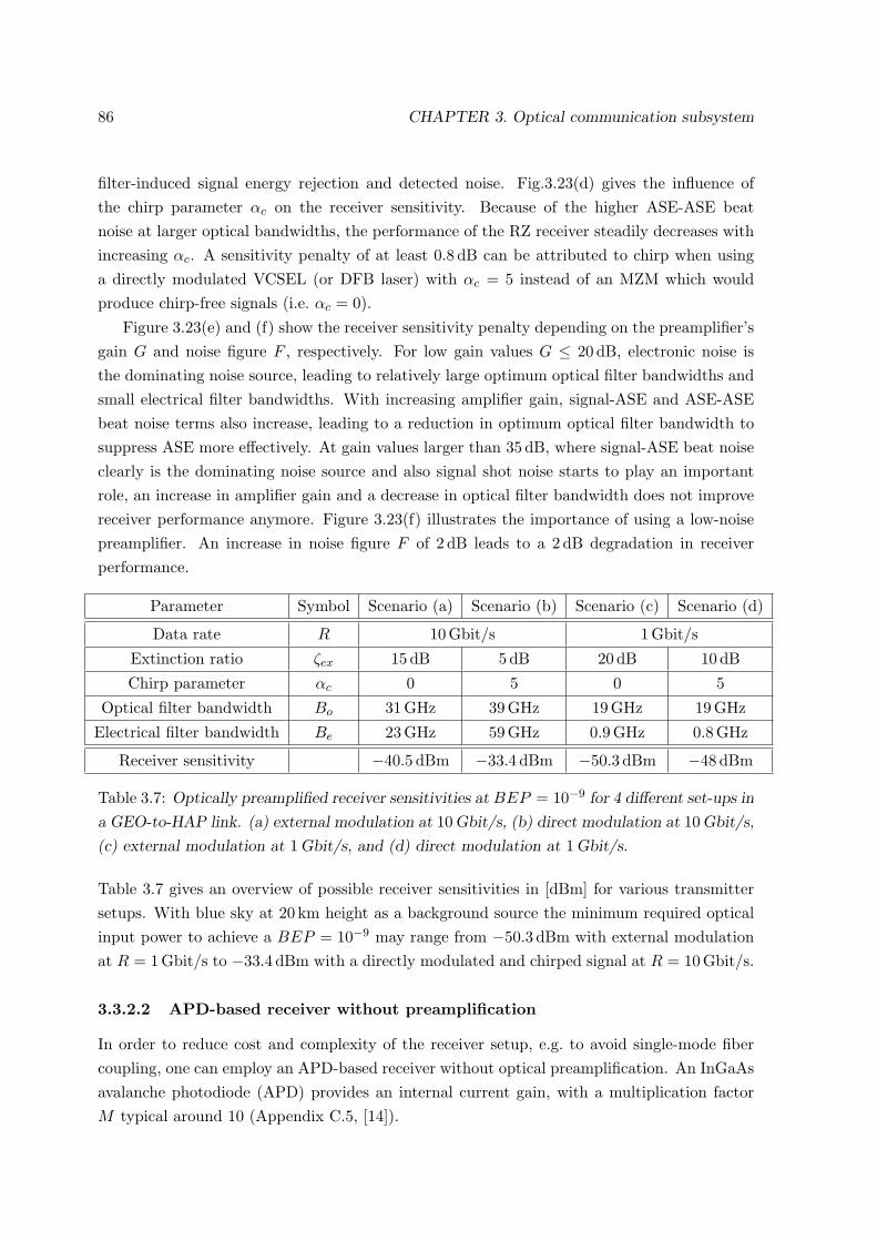
86 CHAPTER 3. Optical communication subsystem
filter-induced signal energy rejection and detected noise. Fig.3.23(d) gives the influence ofthe chirp parameter αc on the receiver sensitivity. Because of the higher ASE-ASE beatnoise at larger optical bandwidths, the performance of the RZ receiver steadily decreases withincreasing αc. A sensitivity penalty of at least 0.8 dB can be attributed to chirp when usinga directly modulated VCSEL (or DFB laser) with αc = 5 instead of an MZM which wouldproduce chirp-free signals (i.e. αc = 0).
Figure 3.23(e) and (f) show the receiver sensitivity penalty depending on the preamplifier’sgain G and noise figure F , respectively. For low gain values G ≤ 20 dB, electronic noise isthe dominating noise source, leading to relatively large optimum optical filter bandwidths andsmall electrical filter bandwidths. With increasing amplifier gain, signal-ASE and ASE-ASEbeat noise terms also increase, leading to a reduction in optimum optical filter bandwidth tosuppress ASE more effectively. At gain values larger than 35 dB, where signal-ASE beat noiseclearly is the dominating noise source and also signal shot noise starts to play an importantrole, an increase in amplifier gain and a decrease in optical filter bandwidth does not improvereceiver performance anymore. Figure 3.23(f) illustrates the importance of using a low-noisepreamplifier. An increase in noise figure F of 2 dB leads to a 2 dB degradation in receiverperformance.
Parameter Symbol Scenario (a) Scenario (b) Scenario (c) Scenario (d)
Data rate R 10 Gbit/s 1 Gbit/s
Extinction ratio ζex 15 dB 5 dB 20 dB 10 dB
Chirp parameter αc 0 5 0 5
Optical filter bandwidth Bo 31 GHz 39 GHz 19 GHz 19 GHz
Electrical filter bandwidth Be 23 GHz 59 GHz 0.9 GHz 0.8 GHz
Receiver sensitivity −40.5 dBm −33.4 dBm −50.3 dBm −48 dBm
Table 3.7: Optically preamplified receiver sensitivities at BEP = 10−9 for 4 different set-ups in
a GEO-to-HAP link. (a) external modulation at 10 Gbit/s, (b) direct modulation at 10 Gbit/s,
(c) external modulation at 1 Gbit/s, and (d) direct modulation at 1 Gbit/s.
Table 3.7 gives an overview of possible receiver sensitivities in [dBm] for various transmittersetups. With blue sky at 20 km height as a background source the minimum required opticalinput power to achieve a BEP = 10−9 may range from −50.3 dBm with external modulationat R = 1 Gbit/s to −33.4 dBm with a directly modulated and chirped signal at R = 10 Gbit/s.
3.3.2.2 APD-based receiver without preamplification
In order to reduce cost and complexity of the receiver setup, e.g. to avoid single-mode fibercoupling, one can employ an APD-based receiver without optical preamplification. An InGaAsavalanche photodiode (APD) provides an internal current gain, with a multiplication factorM typical around 10 (Appendix C.5, [14]).

3.3 Receiver 87
Figure 3.24 sketches the setup of an APD-based receiver. After reception of the RZ-coded data stream, the optical signal which also contains noise due to background light andbooster amplifier ASE is filtered by means of an optical thin film band pass filter. Optical-to-electrical conversion is performed by an APD photodiode module which also incorporates atransimpedance amplifier. After passing a fifth-order Bessel lowpass filter the electrical signalis sampled and an adaptive threshold decision leads to a certain bit error probability BEP .
Because of no single-mode coupling and a reduced number of optical components beforethe APD photodiode, the internal receiver loss is much smaller when compared to that ofthe optical preamplified receiver. It is determined mainly by the insertion loss of the opticalbandpass filter of approximately 1.1 dB.
Parameter Value
Extinction ratio of MZM ε = 20 dBChirp parameter αc = 0
APD multiplication factor M = 10APD noise figure Fapd = 5.5Detector sensitivity S = 0.8 A/WElectrical noise Nel = 10pA/
√Hz
Unmultiplied dark current Id = 10 nA
Electrical filter fifth-order Bessel lowpassElectrical filter bandwidth optimized
Optical filter thin film filterOptical filter bandwidth optimized
Table 3.8: Default parameter set used for simulation of the receiver sensitivity of an APD-based
DD receiver.
APD photodiodemodule
opticalbandpass
electricallowpass
op
tica
lp
ow
er
time
RZ coded data
+
Nback
a Nfs b
thin filmRX data
Figure 3.24: APD-based receiver structure: The optical RZ input field, the background noise
(Nback), and the booster amplifier ASE noise (afsNb) are filtered by an optical bandpass (thin
film)filter. Optical-to-electrical conversion is performed by an APD photodiode which provides
an internal current gain with a multiplication factor M . The receiver module also incorporates
a transimpedance amplifier in combination with a fifth-order Bessel lowpass filter. Sampling
and threshold decision leads to a bit error probability BEP.

88 CHAPTER 3. Optical communication subsystem
For the estimation of the receiver performance I adapted the self-developed simulation toolSimTool (cf. Section 3.3.2.1 and Appendix B) to the APD-based receiver structure: Derivedfrom the formulas given in [14, 26, 67, 113], I expressed the electrical signal after the diodemodule, specified in terms of voltage, as6
s(t) = CM∣∣(ein(t) + nASEb
√afs + nback
)∗ b(t)
∣∣2 ∗ h(t), (3.21)
where ein(t) is the optical input field, M is the APD gain, nASEb is the amplified spontaneousemission from the booster amplifier, afs is the free-space attenuation factor, nb is the back-ground noise, C the conversion gain of the photo diode module (given in [V/W]), b(t) and h(t)are the impulse responses of the optical and electrical filter, respectively.
Three effects contribute to the electrical signal’s variance σ2s(t) [14]: shot noise (according
to signal, dark current, booster ASE, and background noise), beat noise (between signal,booster ASE, and background noise), and thermal noise of the receiver electronics, i.e.
σ2s(t) = σ2
shot,s(t) + σ2shot,d(t) + σ2
shot,ASEb(t) + σ2shot,back(t)
+ σ2s-ASEb(t) + σ2
s-back(t) + σ2ASEb-ASEb(t) + σ2
back-back(t)
+ σ2elec(t). (3.22)
I mathematically modeled the relevant noise term contributions, where the most importantare illustrated in Fig.3.25, as follows:
• The shot noise according to the received signal can be calculated as [14]
σ2shot,s(t) = SR2
TM2Fapde(|(ein ∗ b)(t)|2 ∗ h2(t)), (3.23)
where S in [A/W] is the photodiode’s responsivity, RT is the resistance that convertsthe output current of the photodiode into a voltage, Fapd is the APD noise figure, ande = 1.602 · 10−19 As is the elementary charge of an electron. Because the avalanchemultiplication process is random shot noise is enhanced. Quantitatively this increasecan be expressed by means of a noise enhancement factor (or APD noise figure)
Fapd = kapdM + (1− kapd)(2− 1/M), (3.24)
with kapd = 0.445 for InGaAs [114].
• An APD also generates multiplied dark current shot noise
σ2shot,d = 2eMIDFapdBeR
2T , (3.25)
through avalanche multiplication of dark current charge carriers [14], which is stationaryand independent of the received optical power.
6The operator ∗ represents a convolution (x ∗ y)(t) =∞∫−∞
x(τ)y(t− τ)dτ .

3.3 Receiver 89
• Other, in many cases negligible shot noise contributions (cf. Fig.3.25), arise from boosteramplifier ASE
σ2shot,ASEb = SR2
TM2Fapde(|(nASEb
√afs ∗ b)(t)|2 ∗ h2(t))
= SR2TM
2FapdePASEbBe, (3.26)
and background light
σ2shot,back = SR2
TM2Fapde(|nback ∗ b)(t)|2 ∗ h2(t))
= SR2TM
2FapdePbackBe. (3.27)
Because the expected values of the optically filtered booster ASE and background noiseis time invariant7, they can be expressed as
PASEb = 〈|(nASEb√afs ∗ b)(t)|2〉 = 2mNbafsrb(0), (3.28)
andPback = 〈|(nback ∗ b)(t)|2〉 = 2mNbackrb(0), (3.29)
respectively. Here the factor of 2 accounts for both polarization directions, Nb denotesthe noise power spectral density of the booster amplifier ASE given in [W/Hz], Nback isthe noise power spectral density of the background light in [W/Hz], m is the number ofreceived spatial modes (cf. eqn.(2.49)), afs is the free space attenuation factor, and rb(0)is the value at t = 0 of the optical filter’s autocorrelation function
rb(t) =∫ ∞−∞
b(τ)b?(τ − t)dτ. (3.30)
• Upon detection, the random booster ASE field beats against the signal and against itself,leading to signal-booster ASE beat noise [67]
σ2s-ASEb(t) = 2C2mNbafsM
2Re ∞∫∫−∞
ef (τ)e?f (τ)rb(τ − τ)h(t− τ)h(t− τ)dτdτ, (3.31)
where ef (t) = (ein ∗ b)(t) is the optically filtered input field; and it leads to boosterASE-booster ASE beat noise
σ2ASEb-ASEb = 2C2m2N2
b a2fsM
2
∞∫−∞
|rb(τ)|2rh(τ)dτ. (3.32)
• Similar to booster ASE, also background light generates beat noise terms
σ2s-back(t) = 2C2mNbackM
2Re ∞∫∫−∞
ef (τ)e?f (τ)rb(τ − τ)h(t− τ)h(t− τ)dτdτ, (3.33)
7The expression 〈x(t)〉 is the temporal mean value of x(t).
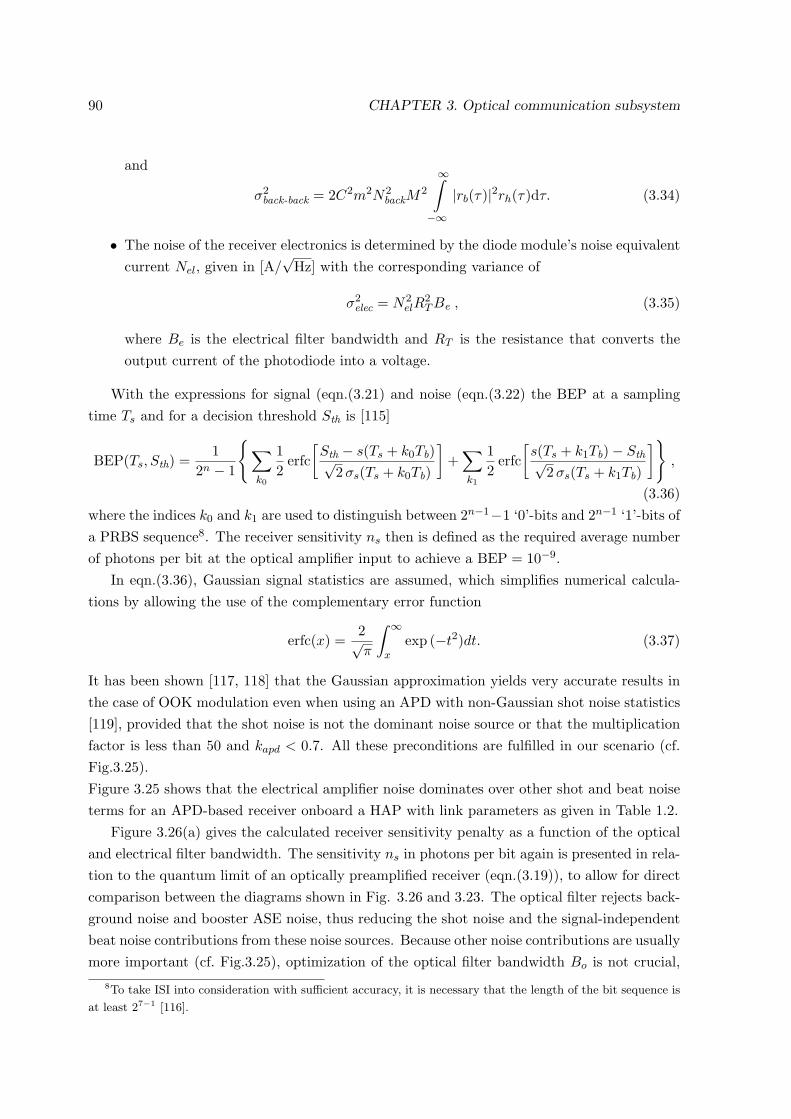
90 CHAPTER 3. Optical communication subsystem
and
σ2back-back = 2C2m2N2
backM2
∞∫−∞
|rb(τ)|2rh(τ)dτ. (3.34)
• The noise of the receiver electronics is determined by the diode module’s noise equivalentcurrent Nel, given in [A/
√Hz] with the corresponding variance of
σ2elec = N2
elR2TBe , (3.35)
where Be is the electrical filter bandwidth and RT is the resistance that converts theoutput current of the photodiode into a voltage.
With the expressions for signal (eqn.(3.21) and noise (eqn.(3.22) the BEP at a samplingtime Ts and for a decision threshold Sth is [115]
BEP(Ts, Sth) =1
2n − 1
∑k0
12
erfc[Sth − s(Ts + k0Tb)√
2σs(Ts + k0Tb)
]+∑k1
12
erfc[s(Ts + k1Tb)− Sth√
2σs(Ts + k1Tb)
],
(3.36)where the indices k0 and k1 are used to distinguish between 2n−1−1 ‘0’-bits and 2n−1 ‘1’-bits ofa PRBS sequence8. The receiver sensitivity ns then is defined as the required average numberof photons per bit at the optical amplifier input to achieve a BEP = 10−9.
In eqn.(3.36), Gaussian signal statistics are assumed, which simplifies numerical calcula-tions by allowing the use of the complementary error function
erfc(x) =2√π
∫ ∞x
exp (−t2)dt. (3.37)
It has been shown [117, 118] that the Gaussian approximation yields very accurate results inthe case of OOK modulation even when using an APD with non-Gaussian shot noise statistics[119], provided that the shot noise is not the dominant noise source or that the multiplicationfactor is less than 50 and kapd < 0.7. All these preconditions are fulfilled in our scenario (cf.Fig.3.25).Figure 3.25 shows that the electrical amplifier noise dominates over other shot and beat noiseterms for an APD-based receiver onboard a HAP with link parameters as given in Table 1.2.
Figure 3.26(a) gives the calculated receiver sensitivity penalty as a function of the opticaland electrical filter bandwidth. The sensitivity ns in photons per bit again is presented in rela-tion to the quantum limit of an optically preamplified receiver (eqn.(3.19)), to allow for directcomparison between the diagrams shown in Fig. 3.26 and 3.23. The optical filter rejects back-ground noise and booster ASE noise, thus reducing the shot noise and the signal-independentbeat noise contributions from these noise sources. Because other noise contributions are usuallymore important (cf. Fig.3.25), optimization of the optical filter bandwidth Bo is not crucial,
8To take ISI into consideration with sufficient accuracy, it is necessary that the length of the bit sequence is
at least 27−1 [116].

3.3 Receiver 91nois
e te
rms
[A²]
signal shot noise shot,sσ²dark current shot noise shot,dσ²
background shot noise shot,backσ²
booster ASE shot noise shot,ASEbσ²
electrical amplifier noise elecσ²
beat noise signal-background s-backσ²
beat noise signal-booster ASE s-ASEbσ²
beat noise booster ASE-background ASEb-backσ²
0 20 40 60 80 100optical filter bandwidth B [R]o
(a)0 20 40 60 80 100
electrical filter bandwidth B [R]e(b)
10-28
10-24
10-20
10-16
10-12
10-28
10-24
10-20
10-16
10-12
Figure 3.25: Noise current terms in an APD-based receiver onboard a HAP for (a)optimum
electrical filter bandwidth (Be = 0.8R) and (b) optimum optical filter bandwidth (Bo = 24R),
assuming blue sky as background source (Nback = 8.867 · 10−28 W/Hz), a booster amplifier
with gain Gb = 30 dB and noise figure of Fb = 6 dB, an electrical noise current density of
Nel = 10 pA/√
Hz, and a link distance of L = 37763 km (affecting the free space loss afs).
as long as it is not chosen too narrow, thereby rejecting significant portions of the input pulseenergy. The dominating noise contributions like electrical amplifier noise, signal shot noise,and multiplied dark current shot noise can be reduced by optimizing the electrical filter band-width Be, which is important for achieving a good receiver sensitivity. In our scenario, usingthe parameters from Tables 1.2 and 3.8, the optimum bandwidths are found at Bo = 24Rand Be = 0.8R, where R represents the data rate. The optimum optical filter bandwidth isrelatively large, due to the high electronic noise which does not depend on Bo. The sensitivitypenalty is 14.4 dB, which is 12.8 dB worse than the performance of the optically preamplifiedreceiver.
Figure 3.23(b) to (f) show the receiver sensitivity penalty γq vs. background noise powerspectral density Nback, extinction ratio ζex, chirp parameter αc, APD multiplication factor M ,and unmultiplied dark current Id. The optical and electrical filter bandwidths were alwaysoptimized for best performance.
Unlike single-mode coupled receivers, APD-based receivers suffer significantly from back-ground radiation, because more than one spatial mode of the background light is receivedby the active area of the photodiode. Therefore, the noise spectral power density Nback fordiffraction limited reception has to be multiplied by a factor m (cf. Section 2.2, eqn.(2.49)),depending on the field of view (FOV) of the receiver. If we assume a very narrow FOVof θFOV = 90µrad, the total noise power spectral density in two directions of polarizationamounts to
Nback,total = 2mNback, (3.38)
with m = 38 (eqn.(2.49)). Figure 3.26(b) presents the sensitivity penalty as a function of thebackground noise power spectral density Nback. In the case of blue sky or Earth as backgroundsource, negligible degradation of receiver performance is found compared to the case wherethere is no background light at all. When directly looking into the Sun, receiver performance

92 CHAPTER 3. Optical communication subsystem
5 10 15 20 25 3014
14.5
15
15.5
16
16.5
17
17.5
0 2 4 6 8 10 12 14 16 18 2014
16
18
20
22
APD multiplication factor M0 100 200 300 400 500
14.2
14.4
14.6
14.8
15
15.2
15.4
15.6
unmultiplied dark current I [nA]d
sensi
tivit
y p
enal
ty [
dB
]re
lati
ve
to q
uan
tum
lim
it
g q
extinction ratio zex
[dB]
direct modulation(DFB-laser, VCSEL)
external modulation(MZM, EAM)
(c)
sensi
tivit
y p
enal
ty [
dB
]re
lati
ve
to q
uan
tum
lim
it
g q
(e) (f)
sensi
tivit
y p
enal
ty [
dB
]re
lati
ve
to q
uan
tum
lim
it
g q
14.5
14.6
14.8
15
15.516
16.517
0.5 1 1.5 2 2.5 3
5
10
15
20
25
op
tica
l fi
lter
ban
dw
idth
Bo
[R]
electrical filter bandwidth Be [R]
(a)
14
16
18
20
22
24
26
10-28
10-26
10-24
10-22
10-20
background noise N [W/Hz]back
sensi
tivit
y p
enal
ty [
dB
]re
lati
ve
to q
uan
tum
lim
it
g q
Earth Sun
blue sky from ground
blue sky at 20km
(b)
decrease of opt. B and Bo e
decrease of optimum Bo
14.4
14.5
14.6
14.7
0 1 2 3 4 5 6 7 8chirp parameter ac
sensi
tivit
y p
enal
ty [
dB
]re
lati
ve
to q
uan
tum
lim
it
g q
(d)
MZM(push-pull)
direct modulation(DFB-laser, VCSEL)
external modulation(MZM, EAM)
increase of optimum Bo
sensitivity penalty [dB]
Figure 3.26: Receiver sensitivity penalty γq of an APD-based receiver at a BEP = 10−9 as a
function of (a) optical filter bandwidth Bo and electrical filter bandwidth Be, (b) background
noise power spectral density Nback, (c) extinction ratio of optical RZ input signal ζex, (d) chirp
parameter αc, (e) APD multiplication factor M , and (d) unmultiplied dark current Id.
will deteriorate by 8 dB.
Other than for optically preamplified detection, for the APD-based RX the optimum filterbandwidths stay virtually constant with varying extinction ratio ζex. Because of the highersignal level for the “0”-bits, the increasing signal shot noise at poorer extinction ratios leads toa sensitivity penalty of 0.8 dB when using directly modulated lasers with ζex = 10 dB insteadof external modulation with ζex = 20 dB.

3.3 Receiver 93
Figure 3.26(d) gives the influence of the chirp parameter αc on the receiver sensitivity.Chirp introduced by intensity modulation leads to a spectral broadening of the received pulsesby a factor of
√1 + α2
c . Therefore, the optimum optical filter bandwidth increases with in-creasing αc. Because the optimum Bo is already large for αc = 0 (so that the signal fieldpasses nearly undistorted) and beat noise terms due to booster ASE and background noise aresmall compared to other noise term contributions, a further increase of Bo leads only to minordegradation of receiver performance. A sensitivity penalty of only 0.11 dB can be attributedto chirp when using a directly modulated laser with αc = 5 instead of an MZM which wouldproduce chirp-free signals (i.e. αc = 5).
Figure 3.23(e) illustrates the receiver sensitivity penalty vs. the APD multiplication factorM . The optimum performance is not attained at the highest possible amplification, since notonly the received signal, but also shot noise and beat noise contributions due to signal, back-ground light, booster ASE, and dark current are enhanced by the factor M . Mathematicallythis behavior is expressed in eqn.(3.24) as a noise enhancement factor Fapd which dependson and increases with M [14, 114]. Therefore also the optimum optical and electrical filterbandwidths decrease with increasing multiplication factor to suppress noise more effectively.
In Fig.3.23(f) I show the receiver sensitivity penalty as a function of the (unmultiplied)dark current Id, illustrating the degradation in receiver performance with increasing darkcurrent shot noise. When the dark current increases by a factor of 10, which due to its strongtemperature dependence may happen if the temperature is increased by approximately 20 K[120, 121], the sensitivity penalty is 0.95 dB.
Parameter Symbol Scenario (a) Scenario (b) Scenario (c) Scenario (d)
Data rate R 10 Gbit/s 1 Gbit/s
Extinction ratio ζex 15 dB 5 dB 20 dB 10 dB
Chirp parameter αc 0 5 0 5
Optical filter bandwidth Bo 24R 32R 37.5R 37.5R
Electrical filter bandwidth Be 0.8R 0.6R 0.8R 0.8R
Receiver sensitivity −30.3 dBm −27.7 dBm −38.4 dBm −37.5 dBm
Table 3.9: APD-based receiver sensitivities for 4 different set-ups in a GEO-to-HAP link. (a)
external modulation at 10 Gbit/s, (b) direct modulation at 10 Gbit/s, external modulation at
1 Gbit/s, and direct modulation at 1 Gbit/s.
Table 3.9 gives an overview of possible receiver sensitivities in [dBm] for various transmittersetups. With blue sky at 20 km height as a background source, the minimum required opticalinput power to achieve a BEP = 10−9 may range from −38.4 dBm with external modulationand at R = 1 Gbit/s to −27.7 dBm with a directly modulated and chirped signal at R =10 Gbit/s.

94 CHAPTER 3. Optical communication subsystem
3.3.2.3 Summary - comparison between optically preamplified and APD-basedreceiver
As shown in the previous section, APD-based receiver offer the following advantages:
• Because noise is governed by electronic noise as well as by signal and dark current shotnoise (cf. Fig.3.25), the optimum optical filter bandwidth Bo can be relatively large -large enough to let the signal field pass undistorted. A decrease in extinction ratio oran increase in chirp does not alter the optimum optical filter bandwidth significantly (cf.Fig.3.26). Therefore, the choice of Bo is less critical than in an optically preamplifiedreceiver (cf. Fig.3.23(a) and Fig.3.26(a)).
• System complexity is greatly reduced in APD-based receivers. Not only the number ofrequired components is less than in an optically preamplified receiver setup (cf. Fig.3.21and Fig.3.24), but also coupling into a single-mode fiber is not necessary.
• Because of low system complexity and fewer components, also reduced costs have to beexpected for the receiver setup.
• If atmospheric turbulence gets too large, i.e. if phasefront perturbations in the receivedwavefront would lead to a significant reduction of the coupling efficiency into the single-mode fiber (cf. Section 2.1.4), an APD-based receiver has to be used.
If high-sensitivity detection is required, an optically preamplified receiver is needed:
• Optically preamplified receivers offer a much better sensitivity than APD-based receivers- only a few dB above the theoretical quantum limit (cf. Fig.3.23) - leading to a significantincrease in transmission distance.
• Noise contributions due to background light are less of a problem (cf. Fig.3.23(b) andFig.3.26(b)), because only one spatial mode (in two directions of polarization) is coupledinto the single-mode fiber [56].
• Optical losses following the amplification process do not degrade the sensitivity, providedthat the receiver works in the signal-ASE or ASE-ASE beat noise limited region [66].
3.4 Link budget
An important issue when assessing the performance of the communication system is the linkbudget of the free-space link, which compares the transmitter’s power less all power losseswithin the system to the required optical power at the input of the receiver. The remainingpower at the receiver basically determines the possible data transmission rate, though this isalso influenced by the modulation format, the acceptable bit error probability, and variousnoise sources.

3.4 Link budget 95
The power budgets which I present in this section are calculated for the GEO-to-HAPscenario, with the aim to compare the link performance
• at data rates of R = 1 Gbit/s and R = 10 Gbit/s,
• when using either an optically preamplified receiver or an APD-based receiver, and
• with chirp-free external modulation (e.g. by means of a proper Mach-Zehnder modula-tor) or with direct modulation (e.g. by using a VCSEL leading to additional spectralbroadening due to chirp).
The detailed set of used parameter values was already given in Table 1.2 for the commu-nication link, and in Table 3.1 and 3.8 for the envisaged receiver setups.
3.4.1 Optical antenna gain
For large transmission distances it is essential to use a well collimated laser beam. A low beamdivergence is achieved with diffraction-limited beams of large diameter, i.e. with spatiallycoherent laser sources and large optical transmit telescopes [41, 37, 14]. Due to the shortwavelength of light, the beam divergence of an optical transmitter can be much smaller thanthat of a microwave source of similar size. The antenna gain can be much higher for opticaltransmitters, e.g. well over 100 dB even for moderate telescope diameters of, e.g., 13.5 cm [28].
The optical antenna gain is defined as the ratio of intensity per solid angle in a beam of(half-angle) beam divergence θ to the equivalent intensity of an isotropic source radiating thesame total power [28]. The intensity, I0, of the optical field produced at a distance l1 from aunit power isotropic radiator is given by
I0 = 1 W/(4πl21). (3.39)
The gain of the optical antenna at a certain angle θ1 off the line-of-sight is then defined as
G(l1, θ1) = I(l1, θ1)/I0, (3.40)
where the gain depends on l1 only in the near field [28].
3.4.1.1 Transmit antenna gain
Based on the theory presented in [28] I calculate the transmit antenna gain for the terminalonboard the HAP and the GEO, assuming an antenna diameter of DTX = 0.135 m. Truncationby the aperture boundary leads to losses in transmitter power and is included in the calculationof the over-all antenna gain. As already mentioned in Section 1.3, I assume an unobscured off-axis mirror transmit telescope (Schiefspiegler) with a beam truncation of αT = DTX/wout =2.24 leading to maximum on-axis gain, with wout being the 1/e2 (intensity) radius of theoutgoing beam.

96 CHAPTER 3. Optical communication subsystem
The on-axis transmit antenna gain is calculated according to [28]
GT = 10 log10
(4πATλ2
gT (αT )), (3.41)
where the first factor 4πAT /λ2 is the well known upper limit of the antenna gain with AT =D2TXπ/4, and gT (αT ) is an efficiency factor accounting for the loss due to truncation, i.e.
gT (αT ) =8α2T
[exp
(−(αT /2)2
)− 1]2. (3.42)
Using these equations, an antenna diameter of DTX = 0.135 m results in a farfield on-axis gainof GT = 108 dB.
3.4.1.2 Receive antenna gain
On the receiver side it is also advantageous to have a high directionality to collect as muchas possible of the transmitter’s power, but also to minimize background light. This can beachieved by using a large telescope at the receiver end [122, 14]. The dimension of the RXtelescope is limited mainly by mass and size constraints dictated by the used platform (HAPor GEO satellite).
In accordance with [122] I assume that the signal source is sufficiently far away so that planewaves impinge on the receiver aperture. For the HAP-from/to-GEO communication scenariothis holds true, because the Rayleigh distance (assuming a telescope diameter of 0.135 m) isapproximately 23.5 km, much smaller than the minimum link distance of L = 35766 km. Then,the antenna gain of the receiving aperture AR can be calculated as
GR = 10 log10
(4πARλ2
), (3.43)
leading to GR = 108.7 dB for a receive telescope diameter of DRX = 0.135 m.
3.4.2 Link loss
The link loss is governed by the free-space loss
afs = 20 log10
(4πLλ
), (3.44)
which is the loss in signal strength of an electromagnetic wave resulting from a line-of-sight pathwith length L through free space, with no obstacles nearby to cause reflection or diffraction[14]. The free-space loss is derived from the ratio PT /PR between transmitted power, PT ,and received power, PR. It accounts for the spreading of transmitted power over a sphericalsurface, PT /(4πL2), which increases with increasing distance L, and it takes into account howwell the receive antenna can pick up power from the incoming electromagnetic wave, i.e.
PR =PT
4πL2
λ2
4π. (3.45)
Additionally, we have to take into account the atmospheric loss due to scattering, absorp-tion, and beam spreading, which was already discussed in detail in Section 2.1.
3.4 Link budget 97
3.4.3 Terminal assembly loss
Beside the losses which occur between transmit and receive telescope, one has to take intoaccount losses that arise directly from nonidealities in the transmitter and receiver setup.Some devices and effects for which additional losses have to be accounted for in the transmitpath are:
Transmitter assembly loss aT is caused by reflections and insertion losses of nonideal op-tical components placed after the optical booster amplifier. Such components may beoptical connectors, collimiating lenses, relay optics, moveable mirrors to achieve point-ing (e.g. the fine pointing mechanism or mirrors for the point ahead angle), or polarizers(e.g. quarter-wave plates). Part of the transmit power might also be used for internalalignment purposes, e.g. for calibration of the tracking system.
Transmit telescope loss aTA is due to aberrations, reflections, or defocus of the emittedbeam. Note that we already accounted for truncation of the beam when calculating thetransmit antenna gain GT .
Pointing loss ap is caused by a misspointing of the transmitted laser beam towards thereceive telescope. It can arise from an error in the calculated point ahead angle or fromuncompensated vibrations onboard the HAP or satellite.
In the receive path the following losses might occur:
Receive telescope loss aRA is due to antenna imperfections like aberrations or reflections.
Coupling loss aco into a single-mode fiber occurs when using an optically preamplified re-ceiver with a single-mode pigtailed EDFA. As discussed in Section 2.1.4, the minimuminsertion loss is 0.9 dB due to mode mismatch, a value that increases with increasingatmospheric turbulence (i.e. increasing phasefront perturbation). Additionally, Fresnellosses due to reflections at the fiber’s input facet might occur.
Receiver assembly loss aR is caused by reflections and absorption losses of nonideal opticalcomponents placed before the APD-photodiode or the optical preamplifier. Such com-ponents may be optical connectors, optical lenses, relay optics, optical filters, duplexers,inline tracking sensors, or polarization filters (e.g. quarter-wave plates).
Tracking loss at is caused by a misspointing of the receive antenna, off from the LOS betweenthe centers of transmit and receive telescope.
3.4.4 Power margin
The system power margin pm is the difference between available signal power and the minimumsignal power needed to achieve a given performance level (i.e. a certain BEP) [123]. In [dB] it

98 CHAPTER 3. Optical communication subsystem
is calculated as
pm = (PT +GT − aT − aTA − ap − afs − aatm − aRA − aR − at +GR)− SRX , (3.46)
i.e. by summing up the average transmit power PT and the antenna gains, and subtracting allloss contributions and the receiver sensitivity SRX .
The power margin is available to compensate for
• the effects of component aging in the transmitter and receiver assembly,
• additional losses which were not accounted for (e.g. an additional pointing loss in thecase of a malfunction in the PAT system), and
• the effects of a time-variant receive power caused by the physical transmission medium(e.g. fading due to atmospheric turbulence) or the platform (e.g. fading due to vibrationsonboard the HAP).
Table 3.10 shows all individual gain and loss contributions for the link budget and the resultingpower margin in a GEO-to-HAP downlink
• at data rates of R = 1 Gbit/s and R = 10 Gbit/s,
• when using either an optically preamplified receiver or an APD-based receiver, and
• with chirp-free external modulation (e.g. by means of a proper Mach-Zehnder modula-tor) or with direct modulation (e.g. by using a VCSEL leading to additional spectralbroadening due to chirp).
The optical filter bandwidths in the receiver are either optimized or, at R = 1 Gbit/s, deter-mined by the available filter technology. The electrical filter bandwidths are always optimizedwith respect to maximum receiver sensitivity. The power margin is calculated according toeqn.(3.46) for a worst case scenario, assuming relatively high losses in the transmit and re-ceive assembly, and (represented by the values in parentheses) for a best case scenario, whereminimum (but technologically feasible) loss values are presumed.
At a data rate of R = 1 Gbit/s a positive link margin is achieved when using an opticallypreamplified receiver. Applying external modulation, the margin may be as large as 9.7 dB.External modulation is also the precondition for obtaining a positive margin using an APD-based receiver. In this case, all losses have to be minimized (i.e. the best case scenario has tobe assumed).
Especially for the APD-based receiver, a larger power margin would be required to guar-antee a long life time of the system. This could be achieved through several measures:
• A straightforward approach would be to increase transmit power. However, the powerconsumption of booster EDFAs with transmit power larger than 40 dBm might be toolarge to be accommodated onboard a HAP or a satellite.

3.4 Link budget 99
Op
tica
lly
pre
amp
lifi
edR
XA
PD
-bas
edR
XP
aram
eter
sS
ym
bol
(a)
(b)
(c)
(d)
(a)
(b)
(c)
(d)
Lin
kdi
stan
ceL
[km
]37
763
Zen
ith
angl
eζ
[]
50
Ext
inct
ion
rati
oζ ex
[dB
]15
520
1015
520
10
Chi
rppa
ram
eter
αc
05
05
05
05
Dat
ara
teR
[Gbi
t/s]
101
101
Opt
ical
filte
rba
ndw
idth
Bo
[GH
z]31
3919
2432
37.5
Ele
ctri
cal
filte
rba
ndw
idth
Be
[GH
z]23
590.
90.
88
60.
8
TX
ante
nna
diam
eter
DTX
[m]
0.13
5
RX
ante
nna
diam
eter
DRX
[m]
0.13
5
av.
tran
smit
pow
erPT
[dB
m]
40
TX
ante
nna
gain
GT
[dB
]10
7.85
TX
asse
mbl
ylo
ssaT
[dB
]2
(1.5
)
TX
tele
sc.
asse
mbl
ylo
ssaTA
[dB
]1
(0.5
)
Poi
ntin
glo
ssap
[dB
]2.
5(0
.5)
Free
-spa
celo
ssafs
[dB
]28
9.72
Atm
osph
eric
loss
aatm
[dB
]0.
35
RX
tele
sc.
asse
mbl
ylo
ssaRA
[dB
]1
(0.5
)
Cou
plin
glo
ssaco
[dB
]1.
3(0
.9)
0
RX
asse
mbl
ylo
ssaR
[dB
]4
(3)
3(1
.5)
Tra
ckin
glo
ssat
[dB
]1
(0.2
)1
(0)
RX
ante
nna
gain
GR
[dB
]10
8.74
Rec
eive
rse
nsi
tivit
ySRX
[dB
m]
-40.
5-3
3.4
-50.
3-4
8-3
0.3
-27.
7-3
8.4
-37.
5
Pow
erm
argi
npm
[dB
]-5
.8(-
0.08
)-1
2.9
(-7.
2)4
(9.7
)1.
72(7
.4)
-13.
7(-
7.7)
-16.
3(-
10.3
)-5
.6(0
.4)
-6.5
(-0.
5)
Fade
leve
lFT
[dB
]0.
22
Surg
ele
vel
ST
[dB
]0.
13
Dyn
amic
rang
e[d
B]
0.35
Tab
le3.
10:
Lin
kb
ud
get
sfo
rG
EO
-to-
HA
Pd
own
lin
ksc
enar
ios
(TX
...t
ran
smit
ter,
RX
...r
ecei
ver)
wit
ha
targ
etBEP
=10−
9.
Th
ep
ower
mar
gin
isgiv
enfo
ra
wor
stca
sesc
enari
o(a
nd
inpar
enth
eses
for
ab
est
case
scen
ario
).F
ade
and
surg
ele
vels
(i.e
.th
ep
ossi
ble
dynam
ic
ran
ge)
are
take
nfr
omS
ecti
on2.
1at
afa
de
(an
dsu
rge)
pro
bab
ilit
yof
10−
2an
dat
no
angu
lar
poin
tin
ger
ror
(α=
0).

100 CHAPTER 3. Optical communication subsystem
• Figure 3.27(a) shows the power margin at R = 1 Gbit/s as a function of the transmitand receive telescope diameters when using external modulation and an APD-basedreceiver (SRX = −38.4 dBm at BEP = 10−9). With increasing antenna diameter alsothe antenna gain increases, leading to a larger power margin9. Antenna diameters ofDTX = DRX = 0.2 m instead of 0.135 m would enable power margins larger than 7 dB.
• A reduced zenith angle (compared to the default zenith angle of ζ = 50) would havean advantageous effect on the power margin (cf. Fig.3.27(b)). The smaller the zenithangle ζ, the shorter is the link distance L (through the atmosphere). This leads to areduced free space loss, a smaller atmospheric loss due to absorbtion and scattering, lessbackground noise due to blue sky, and to less fading.
• Reducing the data rate leads to a reduction of the required minimum receive power. Incase of the APD-based receiver a decrease of the data rate to R = 100 Mbit/s improvesthe power margin by some 5.5 dB (cf. Fig.3.27(c)).
-4 -2
0
2
4
6
transmit telescope diameter D [m]TX
0.1 0.12 0.14 0.16 0.18 0.20.1
0.12
0.14
0.16
0.18
0.2
rece
ive
tele
sco
pe
dia
met
er D
[m
]R
X
(a)
0 10 20 30 40 50 60 70-0.4
0
0.4
0.8
1.2
po
wer
mar
gin
[d
B]
zenith angle [°]z
(b)
10 102 1030
2
4
6
8
10
data rate R [Mbit/s]
po
wer
mar
gin
[d
B]
(c)powermargin [dB]
Figure 3.27: Power margin pm (for a GEO-to-HAP scenario using external modulation at
R = 1 Gbit/s and an APD-based receiver) calculated according to eqn.(3.46) as a function of
(a) receive and transmit telescope diameter, (b) zenith angle, (c) data rate.
3.4.5 Influence of fading on the link budget
As already discussed in Section 2.1.2, turbulent motion of the atmosphere due to temperatureand pressure gradients causes disturbances in the atmosphere’s refractive index, leading totime-depending variations of the received signal (i.e. fades and surges). When establishing thelink budget, one has to quantify the power loss caused by these fluctuations to figure out howmuch additional power is required to compensate for these scintillation effects. Mathematically,the fading-induced power reduction can be taken into account via an additional power penaltyin the link budget and by defining an outage probability with which the link can not be closed.
9In the case of an optically preamplified RX and an atmospheric channel, the increase in antenna diameter is
accompanied by a decrease in coupling efficiency, which, in our scenario, is negligible compared to the additional
antenna gain (cf. Fig.2.16 and Section 2.1.4).

3.4 Link budget 101
The probability of a surge - as shown in Fig.2.12(b) - is very small, and will therefore notsaturated the optical preamplifier or destroy the used (APD) photodiode.
3.4.5.1 Loss based on “long term” average BEP
The time scale of power fluctuations at the receiver depends on the velocity of the turbulenteddies transversal to the optical beam (cf. Section 2.1.2 and Appendix A.2), mathematicallyexpressed by the correlation time [37]
τch =ρchvt, (3.47)
where ρch is the transverse correlation width and vt is the mean wind speed transverse tooptical beam as given by eqn.(A.26). The correlation width is the 1/e2 point of the normalizedcovariance function of intensity, which in turn describes how the intensity fluctuations at onepoint in the beam are correlated with those at another point [37]. The transverse correlationwidth for an uplink path is typically tens of meters or more, while for a downlink propagationpath it is typically in the order of 5 to 15 cm [37]. For our scenario (i.e. under weak turbulenceconditions) it can be approximated by the empirical formula [37]
ρch =
√λ
45 · 103 m sec (ζ)2π
10
1 +(h−7500 m
2500 m)2 , (3.48)
which, at the wavelength of λ = 1550 nm, the altitude h = 20 km, and the zenith angle ζ = 50
leads to ρch = 5 cm. The turbulence correlation time is therefore τch = 418µs in the case of aUAV with velocity vHAP = 11 km/min, and τch = 26 ms in the case of a quasi-geostationaryHAP (vHAP = 0). Because this time scale is much smaller than the bit duration, the opticalpower level of the received signal is constant over a large number of bits. Using the receivermodels described in Section 3.3, a relevant “short term” BEP (depending on the actual receivedpower) can be calculated.
In order to assess the system performance influenced by atmospheric fading sometimesa “long term” average bit error probability BEP is used in literature [124, 125, 126]. It isdefined as the “short term” bit error probability BEP (P ) averaged over all possible values ofreceived optical power P , i.e.
BEP =∫ P
0BEP (p)p(p)dp, (3.49)
with p(p) being the probability density function of P . Possible channel models, based on alognormal PDF (eqn.(2.19)) for weak turbulence and on a gamma-gamma PDF (eqn.(2.20))for strong turbulence, were already discussed in Section 2.1.2.
Because the atmospheric channel is a slow fading channel, i.e. the correlation time τch
(eqn.(3.47)) is large compared to the bit duration, the average “long-term” BEP is of virtuallyno significance. Very high BEPs during a certain amount of time will be canceled out by
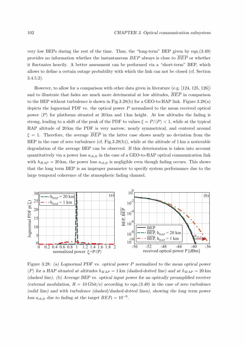
102 CHAPTER 3. Optical communication subsystem
very low BEPs during the rest of the time. Thus, the “long-term” BEP given by eqn.(3.49)provides no information whether the instantaneous BEP always is close to BEP or whetherit fluctuates heavily. A better assessment can be performed via a “short-term” BEP, whichallows to define a certain outage probability with which the link can not be closed (cf. Section3.4.5.2).
However, to allow for a comparison with other data given in literature (e.g. [124, 125, 126])and to illustrate that fades are much more detrimental at low altitudes, BEP in comparisonto the BEP without turbulence is shown in Fig.3.28(b) for a GEO-to-HAP link. Figure 3.28(a)depicts the lognormal PDF vs. the optical power P normalized to the mean received opticalpower 〈P 〉 for platforms situated at 20 km and 1 km height. At low altitudes the fading isstrong, leading to a shift of the peak of the PDF to values ξ = P/〈P 〉 < 1, while at the typicalHAP altitude of 20 km the PDF is very narrow, nearly symmetrical, and centered aroundξ = 1. Therefore, the average BEP in the latter case shows nearly no deviation from theBEP in the case of zero turbulence (cf. Fig.3.28(b)), while at the altitude of 1 km a noticeabledegradation of the average BEP can be observed. If this deterioration is taken into accountquantitatively via a power loss ach,lt in the case of a GEO-to-HAP optical communication linkwith hHAP = 20 km, the power loss ach,lt is negligible even though fading occurs. This showsthat the long term BEP is an improper parameter to specify system performance due to thelarge temporal coherence of the atmospheric fading channel.
0 0.2 0.4 0.6 0.8 1 1.2 1.4 1.6 1.8 20
5
10
15
20
25
30
normalized power =P/ Pñáx
log
no
rmal
PD
F p
(
)x
h = 20 km
h = 1 kmHAP
HAP
(a)
-56 -52 -48 -44 -40 -3610
-10
10-8
10-6
10-4
10-2
100
received optical power P [dBm]
BE
P, B
EP
BEPBEP, h = 20 km
BEP, h = 1 kmHAP
HAP
(b)
ach,lt
Figure 3.28: (a) Lognormal PDF vs. optical power P normalized to the mean optical power
〈P 〉 for a HAP situated at altitudes hHAP = 1 km (dashed-dotted line) and at hHAP = 20 km
(dashed line). (b) Average BEP vs. optical input power for an optically preamplified receiver
(external modulation, R = 10 Gbit/s) according to eqn.(3.49) in the case of zero turbulence
(solid line) and with turbulence (dashed/dashed-dotted lines), showing the long term power
loss ach,lt due to fading at the target BEPt = 10−9.

3.4 Link budget 103
3.4.5.2 Loss based on “short term” instantaneous BEP
As already discussed in Section 2.1.2, surges and fades of the received optical power have tobe expected with a certain probability in a GEO-to-HAP link, leading to a certain dynamicrange the system has to cope with. Thus, the characterization of fading-induced losses basedon a “long-term” average BEP (leading to a power loss of ach,lt ≈ 0 dB) is not sufficient.
Slow fading (compared to the bit duration) also occurs in fiber-based wavelength divi-sion multiplexing (WDM) systems, due to polarization mode dispersion (PMD) [33, 127] ordue to coherent crosstalk between adjacent channels [128]. Like in the atmospheric channel,measurement and calculation techniques based on an average BEP are insufficient becausethe occurrence of error-bursts will most likely be averaged out [128]. System performanceis therefore often characterized by an outage probability, which is the probability that thecommunication link can not be closed [129].
Here I want to adopt this approach and evaluate the quality of the communication link overthe dynamic atmospheric channel via a “short term” (instantaneous) BEP that is achievedduring a relatively short time period and allows to comprehend the fade statistic more precisely.The outage probability pBEP describes the probability by which the BEP is larger than acertain target value BEP t (achieved at an optical power Pt) after the optical receive powerP was multiplied by a factor ach,st. This factor ach,st can be interpreted as a “short term”power loss that has to be compensated for, so that the BEP is larger than BEP t only witha probability pBEP . Mathematically, this may be expressed as
pBEP = P (BEP > BEPt) (3.50a)
pBEP = P (ach,stP ≤ Pt) (3.50b)
pBEP = P
(P
Pt≤ 1ach,st
). (3.50c)
The power loss factor ach,st can be calculated via the cumulative distribution function (CDF)of ξ = P/Pt, given as
pBEP = Fξ
(1
ach,st
)= P
(P
Pt≤ 1ach,st
)=∫ 1/ach,st
−∞p(p)dp. (3.51)
If we assume a lognormal PDF p(p), the closed form solution for eqn.(3.51) according to [37]is given as
pBEP = 0.5
1 + erf
0.5σ2I + ln
(1/ach,st
Pt
)√
2σ2I
, (3.52)
where erf(x) is the error function (eqn.(A.54) and σ2I is the scintillation index (as described
in Section 2.1.2, A.5, and A.6), leading to
ach,st =[exp
[erf−1(2pBEP − 1)
√2σ2
I − 0.5σ2I
]]−1
. (3.53)
For the GEO-to-HAP scenario the value for ach,st can also be found in Fig.2.13. With aprobability of pBEP = 10−2 it amounts to ach,st = 0.22 dB (cf. Table 3.10).

104 CHAPTER 3. Optical communication subsystem
3.4.6 Influence of forward error correction coding on the link budget
The calculated power margins in Table 3.10 show the feasibility of an optical communicationlink between satellite and HAP at the data rate of R = 1 Gbit/s. At larger data rates (e.g. atR = 10 Gbit/s) additional measures have to be found to allow for a positive link margin.
In terrestrial fiber-based systems, forward error correction (FEC) coding (also called chan-nel coding) is one possibility to improve the quality of the communication, regardless of thephysical origin of transmission degradations [68]. It enables the receiver to detect and correcterrors without requesting retransmission of the original information. With FEC, the data se-quence is fed to an encoder which inserts redundant bits, thereby outputting a longer sequenceof code bits, called a codeword. Such codewords are then transmitted to a receiver which usesa suitable decoder to extract the original data sequence [130].
For terrestrial systems the ITU has standardized a 7% coding overhead (to guaranteeinteroperability of systems) [131], which in our case would lead to an effective data rate ofR = 10.7 Gbit/s. The standard FEC (SFEC) scheme uses the ITU standard Reed Solomoncode RS(255,239), while in proprietary enhanced FEC (EFEC) schemes several codes areserially concatenated with a certain interleaving depth and some iterations of decoding areused to improve the error correction capability. Figure 3.29 compares the performance ofSFEC to EFEC [132]. The decoded BEP is given vs. the channel BEP (cf. Fig.3.29(a)) andvs. the optical signal-to-noise ratio (OSNR) (cf. Fig.3.29(b)). The OSNR is defined as [33]
OSNR =P
2BrefN0, (3.54)
where P is the average signal power, Bref is an optical reference bandwidth (e.g. 0.1 nm), andN0 is the noise power spectral density in each polarization. Standard FEC is able to correctBERs from 4 ·10−4 to 10−9 providing a coding gain of 4.9 dB, while EFEC corrects BERs from2.5 · 10−3 to 10−9 which equals a coding gain of 6.4 dB. Forward error correction devices atdata rates up to 10.7 Gbit/s are commercially available for example from Intel, Agere, AMCC,or Vitesse [133].
Reed Solomon codes
Beside optical communications, Reed Solomon codes are used in a wide variety of commercialapplications, most prominently in CDs and DVDs, in data transmission technologies such asDSL, and broadcast systems such as DVB. The RS(N ,K) codes are systematic linear blockcodes [130, 134], where K is the number of data symbols, one symbol consisting of q bits, whichare encoded to a codeword consisting of N = 2q − 1 symbols. They are block codes becausethe original message is split into fixed length blocks and each block is split into q bit symbols,linear because each q bit symbol is a valid symbol, and systematic because the transmittedinformation contains the original data with extra N − K “parity” symbols appended. The

3.4 Link budget 105d
eco
ded
BE
R
channel BER
standard FECenhanced FEC
no FEC
10-1
10-3
10-5
10-7
10-9
10-11
10-13
10-15
10-1
10-3
10-2
10-4
dec
od
ed B
ER
optical SNR [dB]
standard FECenhanced FEC
no FEC
10-1
10-3
10-5
10-7
10-9
10-11
10-13
10-15
2 4 6 8 18 20141210 16
(a) (b)
Figure 3.29: Performance of standard FEC (SFEC) and enhanced FEC (EFEC) [131, 132].
decoder can correct up to [130]
T = bN −K2c, (3.55)
symbol errors in the code word. Given that errors may only be corrected in units of sin-gle symbols, Reed-Solomon decoders are also able to correct burst errors which is especiallyimportant for fading channels.
The ITU standardized RS(255,239) works with q = 8 bit symbols [131], leading to an errorcorrection capability of maximal
t = bq · N −K2c, (3.56)
i.e. 64 erroneous bits per codeword. At a data rate of 10.7 Gbit/s this would lead to a maximumallowed burst error length of 5.98 ns. This can be further increased by using block interleaving[130]. A 16-way interleaved RS(255,239) code that can correct error bursts of up to 1024 bitsis recommended by ITU-T standard G.975 [135]. In such a code, 16 encoders generate 16codeword blocks in parallel. These 16 rows of codewords are transmitted column-wise suchthat long bursts of errors get distributed into multiple codewords. At R = 10.7 Gbit/s the 1024correctable bits correspond to a duration of 95.7 ns, which is still very short when compared tothe milliseconds to microseconds time scale of power fluctuations (cf. eqn.(3.47 and Fig.2.13).Events, during which more than 1024 consecutive bits are disturbed lead to a fading inducedoutage. Therefore, the link has to be dimensioned to meet the worst case BEP requirementsand to fail only with a certain probability.
In the following two subsections I define parameters, i.e. the loss due to temporal fluctua-tions and an effective “short term” loss when using FEC, to quantitatively assess how forwarderror correction may act favorable on the power margin. As an example, I calculate thesevalues for the GEO-to-HAP link assuming Reed Solomon RS(255,239) coding as standardizedby the ITU.
106 CHAPTER 3. Optical communication subsystem
3.4.6.1 Loss due to temporal fluctuations
Knowledge of the mean fade time helps to select a suitable FEC device, as channel coding getsmore and more ineffective if too many consecutive bits are affected by fading [129, 126]. If thenumber of consecutive erroneous bits is larger than the burst error correction capability of thecode, no gain due to coding can be achieved anymore. Similar to Section 3.4.5 a loss factorach,t can be defined by which the transmitted power has to be increased in order to reduce themean fade time below a certain target value tf,BEP . The mean fade time 〈tf 〉 during whichthe (“short term”) BEP is larger than a certain target BEPt should be smaller than tf,BEP ,leading to
tf,BEP = 〈tf (BEP > BEPt)〉 (3.57a)
tf,BEP = 〈tf (ach,tP ≤ Pt)〉 (3.57b)
tf,BEP =⟨tf
(P
Pt≤ 1ach,t
)⟩. (3.57c)
According to [37], eqn.(3.57) can be expressed as
tf,BEP =⟨tf
(P
Pt≤ 1ach,t
)⟩=
P(PPt≤ 1
ach,f
)⟨n(PPt≤ 1
ach,t
)⟩ , (3.58)
where 〈P (x ≤ y)〉 is the probability of fade and 〈n(x ≤ y)〉 is the expected number of fadesper second for x staying below a threshold value y (cf. Section A.10). In the case of weakturbulence, where a lognormal PDF can be assumed and using the mathematical expressionsfor the probability of fade and the number of fades as given in Appendix A, eqn.(3.58) reads
tf,BEP =1
2ν0exp
[0.5σ2
I + ln(
1/ach,t
Pt
)]2
2σ2I
1 + erf
0.5σ2I + ln
(1/ach,t
Pt
)√
2σ2I
, (3.59)
using the error function erf(x) (eqn.(A.54)), the quasi-frequency ν0 (eqn.(A.66)), and thescintillation index σ2
I (cf. Section 2.1.2, A.5, and A.6).
Loss due to temporal fluctuations when using RS(255,239) coding
Figures 2.12(d),(f) and Fig.2.13(d),(f) visualize the results of eqn.(3.59) for the uplink and thedownlink, respectively. In the case of a GEO-to-UAV downlink (at a data rate of 10 Gbit/sand a target BEP of 10−9) the transmitted power would have to be increased by ach,t ≈ 12 dBto be able to correct all burst errors when using a 16 times interleaved RS(255,239) FEC coderand to achieve a negligible outage probability. These 12 dB would be a very large loss to befully compensated.

3.4 Link budget 107
3.4.6.2 Loss based on “short term” BEP when using FEC
The coding gain gch,FEC of an FEC device describes the reduction in required optical receivepower necessary to achieve a certain target BEP when compared to a system without FEC[132]. The coding gain as specified by the manufacturers of FEC devices is valid only fornon-fading channels, i.e. for non-correlated bit errors. When error bursts can not be correcteddue to fading, FEC offers no gain at all. This means that at 10 Gbit/s the link can not beclosed with a certain outage probability pFEC .
In the atmospheric fading channel the number of bits over which the received power Pis constant can be estimated by R · τch, where R is the data rate and τch is the turbulencecorrelation time as given by eqn.(3.47). If the length of one codeword q · N is much smallerthan R · τch, the number of erroneous bits can be calculated as
te = qN ·BEP for qN Rτch, (3.60)
where BEP, the instantaneous “short term” bit error probability, is a random variable. There-fore, the correction of te = qN ·BEP ref errors (at a defined BEP value BEP ref ) to a numberof tt = qN · 10−9 errors is not possible with a certain probability (cf. eqn.(3.50), eqn.(3.51)),i.e.
pFEC = P (BEP > BEPref ),
pFEC = P (ach,FECP ≤ Pref ) ,
pFEC = P
(P
Pt≤
Prefach,FECPt
),
pFEC = F
(Pref
ach,FECPt
),
pFEC =∫ Pref
ach,FECPt
−∞p (p) dp,
pFEC =∫ Pref
ach,FECPt
−∞
1
p√
2πσ2I
exp
−[ln(
Pref
ach,FECPt
)+ 0.5σ2
I
]2
2σ2I
dp,pFEC = 0.5
1 + erf
0.5σ2I + ln
(gch,FEC
Pref
〈P 〉
)√
2σ2I
, (3.61)
where pFEC denotes the probability with which BEP ≤ BEPref is not fulfilled, i.e. the outageprobability of the link. However, the “short-term” loss as defined by eqn.(3.53) can be reducedby using FEC, because the required target BEP is larger than without error correction coding,i.e. BEPref > BEPt. The effective “short-term” loss using FEC can then be expressed as (cf.eqn.(3.53))
ach,FEC =[exp
[erf−1(2pFEC − 1)
√2σ2
I − 0.5σ2I
]]−1 PrefPt
, (3.62)
with Pref < Pt.

108 CHAPTER 3. Optical communication subsystem
Loss based on “short term” BEP when using RS(255,239) coding
To assess the loss ach,FEC when using RS(255,239) coding I first want to calculate the theo-retical lower bound for the achievable BEP, i.e. in the case of no atmospheric turbulence orif an infinitely long interleaver would be available so that all burst errors could be corrected.An RS(N ,K) code is capable of correcting T symbol errors (where each symbol consists of qbits), so the BEP is lower bounded with [130, 136]
BEPmin =T
Nq
[1−
T∑i=0
(N
i
)(1− (1−BEP )q)i(1−BEP )q(N−i)
]. (3.63)
For the RS(255,239) code, BEPmin is illustrated in Fig.3.30(a) (dashed line), showing a codinggain of gch,FEC = 4.9 dB at a BEP = 10−9 when compared to the short term BEP of anuncoded system (solid line). This result is in full accordance with the coding gain as specifiedby the manufacturers of FEC devices (cf. Fig.3.29(b)).
Figure 3.30(b) illustrates the loss ach,FEC (eqn.(3.62)) based on the “short term” BEPwhen using the RS(255,239) code with increasing strength of turbulence (i.e. with increasingscintillation index) for various probability values pFEC . At σ2
I = 0 no additional power isrequired to close the link at 10.7 Gbit/s when using FEC. At increased turbulence the link canonly be closed with a certain probability. Some 5 dB of additional optical power have to beavailable for example at σ2
I = 0.1 to close a link with an outage probability of pFEC = 10−12.If these additional 5 dB are not available, the link fails.
I have just shown that using FEC, error free optical communication (i.e. at a BEP = 10−9)between satellite and HAP is possible at the data rate of R = 10.7 Gbit/s with a certain outageprobability. This probability can be enhanced by various additional measures that go beyondof just increasing the transmit power of the antenna diameters:
• A more advanced channel coding scheme than RS coding could be used, which is ableto correct a larger number of erroneous consecutive bits. Interleaving, i.e. the nestingof a number of code words, can increase the burst error correction capability of a code.However, in the case of a large temporal coherence of the fading channel, i.e. for a slowfading channel like the atmosphere, the interleaving depth has to be very large to beeffective [137].
• One could additionally implement an ARQ (automatic repeat request) technique toperform the remaining error corrections. There, erroneously received messages (which ischecked by a number of parity bits) are simply retransmitted if this is requested by thereceiver [130].
3.4.7 Summary - link budget
The previous sections showed that in a GEO-to-HAP communication scenario, the optical linkcan be closed at the data rate of 1 Gbit/s when using either an optically preamplified receiver,

3.4 Link budget 109
-48 -47 -46 -45 -44 -43 -42 -41 -40 -39 -3810
-12
10-10
10-8
10-6
10-4
10-2
optical receive power P [dBm]
(short
ter
m)
BE
P
(a)
gch,FEC
0 0.1 0.2 0.3 0.4 0.5-20
-15
-10
-5
0
5
(short
ter
m)
loss
a [
dB
]ch
,FE
C
scintillation index sI
2
(b)
p = 10FEC
-2
p = 10p = 10p = 10
FEC
FEC
FEC
-6
-9
-12
no FEC, no fadingFEC, no fading
Figure 3.30: (a) (Short term) BEP with and without FEC vs. optical receive power, showing
the coding gain gch,FEC . (b) Loss ach,FEC based on “short term” BEP vs. scintillation index
σ2I (as a function of the outage probability pFEC) according to eqn.(3.62) in the case of a GEO-
to-HAP communication link (assumptions: R = 10.7 Gbit/s, external modulation, optically
preamplified receiver, weak turbulence).
or an APD-based receiver in combination with external modulated signals. Several measuresfor increasing the power margin were discussed, which included the use of larger telescopediameters, the increase in transmit power, the establishment of the link at small zenith angles,or even a reduction in data rate.
I discussed two different power loss parameters to account for the effect of atmosphericfading on the link budget calculations, one based on an average “long term” BEP which isinsufficient due to the large temporal coherence of the fading channel, the other based on aninstantaneous (random) “short term” BEP showing the temporary power loss which occurs ata certain probability.
For optical communication links at large data rates such as 10 Gbit/s, a positive powermargin can only be achieved when using additional sensitivity enhancement measures such asforward error correction (FEC). Even then, the correction of bit errors in order to achieve acertain target BEP can only be guaranteed with a certain probability, because atmosphericturbulence temporary leads to deep fades, causing burst errors which can not be corrected.In this case, additional measures like automatic repeat request (ARQ) techniques - where lostdata is retransmitted - are recommended.

110 CHAPTER 3. Optical communication subsystem

Chapter 4
Summary
“Science is like a blabbermouth who ruins a movie by tellingyou how it ends. Well, I say that there are some things wedon’t want to know. Important things!”
N. Flanders, cartoon character (Simpsons)
In this study I assessed the performance of an optical HAP-to-satellite link at the wave-length of 1550 nm. The scope of this work was to develop the methodology for designing theoptical communication subsystem in the Gb/s-regime for such a scenario.
Chapter 2 dealt with the channel model of the communication link through the atmosphere:In Section 2.1 I discussed several impairments which are caused by atmospheric turbulence.Based on analytical models and measurements given in literature for ground-to-satellite links[37, 34, 25, 26], I developed mathematical models which I tailored to the envisaged pathbetween a HAP and a GEO satellite at various zenith angles. This was necessary becausetraditional models do not account correctly for the reduced amount of atmosphere at highaltitudes and they do not include the effect of a pointing error and of beam wander in the caseof strong turbulence. They only treat the case of a plane wave or a spherical wave but not thatof a Gaussian beam shape and they are simply inadequate for high UAV moving speeds. Mycalculations showed that compared to a ground-to-satellite link, the impact of the atmosphereon the propagating laser beam is greatly reduced.
In Section 2.2, I calculated the background noise power density which is added to theoptical signal and caused by background radiation from Earth and from sky. Other than in[34, 26], I did not only take into account the self-emission but also the reflected sunlight fromthe Earth’s surface. In the case of sky radiance, I incorporated that the scattered radiationdecreases with increasing height. Background light, quantitatively characterized by a spectralpower density, acts as an additional noise source within the system.
Chapter 3 treats the design and the performance estimation of the optical communicationssubsystem: In Section 3.1, I addressed the impact that the use of various optical modulationformats has on the performance and complexity of the communication subsystem. Basedon calculated receiver sensitivities and on a performance/complexity trade-off, I selected themost promising modulation format for our scenario, which is return-to-zero (RZ) intensitymodulation.
In Section 3.2, dealing with the transmitter setup, I presented measurements characterizinga new and potentially important semiconductor laser source at the wavelength of 1550 nm,
111

112 CHAPTER 4. Summary
namely a vertical-cavity surface-emitting laser (VCSEL). Modifying the electrical package ofthe lasers by means of an RC-element allowed for direct modulation at 10 Gbit/s.
For a comparison of the performance of two different direct-detection receivers, namelythe optically preamplified and the APD-based receivers, I calculated the receiver sensitiviy(cf. Section 3.3.2.3), which is the minimum optical input power required to achieve a bit-error-probability of 10−9. While for an optically preamplified receiver the sensitivity is only1.6 dB above the theoretical quantum limit, the APD-based receiver shows a sensitivity whichis 12.8 dB worse than the performance of the optically preamplified receiver. However, theAPD-based receiver has the advantage of reduced system complexity, because coupling into asingle-mode fiber is not required.
In Section 3.4, I presented detailed link budget calculations for a GEO-to-HAP link, whichtook into account all possible losses that can occur in the transmitter, the channel, and thereceiver. My computations show that a positive power margin can be achieved at a datarate of 1 Gbit/s. At 10 Gbit/s the use of forward-error-correction (FEC) would be required. Iintroduced quantitative parameters, i.e. the average (“long-term”) BEP and the instantaneous(“short-term”) BEP, which allow to demonstrate the advantageous effect of FEC, as well asthe detrimental influence of power fluctuations caused by atmospheric turbulence.
4.1 Developed tools
Transmitter Channel Receiver+
backgroundnoise
AtmosPhD+ SimToolPhD+
LinkBudgetPhD+
target BEP
power margin
simulation software
Figure 4.1: Overview of software bundle developed in the course of this thesis.
During this study I developed a set of software tools which allow for the performance as-sessment of optical communication links (at various zenith angles) through the atmospherewhen using intensity modulation (cf. Fig.4.1). These Matlab tools are not limited to com-munication scenarios from or to a HAP, but can also be used to evaluate up- and downlinksbetween ground stations and satellites.

4.1 Developed tools 113
The atmospheric channel model, which I derived in Section 2.1, is implemented into theprogram AtmosPhD+. It allows to characterize the influence turbulence has on a (Gaussian)laser beam propagating on a path through the atmosphere at various zenith angles. The set ofrequired input parameters and calculated output parameters is shown in Fig.4.2. Underlyingmathematical models are described in Section 2.1 and Appendix A.
HAP altitude
satellite altitude
HAP telescope diameter
satellite telescope diameter
HAP velocity
geodetic latitudezenith angle
fading threshold
surge threshold
structure constant at ground
wind speed at ground
selection uplink/downlinkselection untracked/tracked/tip-tilt corr.
selection aperture averaging on/off
h
h
D
D
v
geo
F
S
C ²(0)
v
HAP
SAT
HAP
SAT
HAP
T
T
n
wind
ζα
d
λ
normalized pointing error
divergence factor
communication wavelength
n
f
Fried parameter r
beam spread loss a
coupling loss into SMF a
power coupling efficiency into SMF²
probability of fade P(F>F )
probability of surge P(S>S )
expected number of fades per second n(F )
mean fade time
0
bs
co
T
T
T
ηscintillation index σ
α
β
θ
I
á ñ
t
angular pointing error
variance of angle of arrival fluctuations ²
effective divergence angle
indicator weak/strong turbulence
á ñ
á ñ
f
a
effAtm
osP
hD
+
Figure 4.2: Input and output parameters of software tool AtmosPhD+.
The performance of a receiver is quantitatively characterized by its sensitivity, which isthe average optical input power required to achieve a certain bit error probability. I expandedthe functionality of the in-house developed simulation software Simtool [66, 68], which allowsto calculate the receiver sensitivity of an optically preamplified receiver when using intensitymodulation, to APD-based receivers (cf. Section 3.3.2.2 and Appendix B). The actual version,SimToolPhD+, now also allows to take into account noise from background radiation (cf.Section 2.2) and ASE noise from the booster amplifier. The set of required input parametersand calculated output parameters of SimToolPhD+ is shown in Fig.4.3. When knowingthe optical transmit power, all losses and gains along the transmission path, as well as thereceiver sensitivity, one can calculate the power margin at a certain target BEP. As I haveshown in Section 3.4.5 and Section 3.4.6, this power margin can only be guaranteed witha certain probability in a communication link through the atmosphere, because turbulenceleads to power fluctuations at the input of the receiver. I implemented the calculation of thelink budget into a Matlab tool, LinkBudgetPhD+, which takes into account the (detrimental)effects of fading and the (possible) gain due to forward-error-correction (FEC) in the casethat burst errors don’t cause a link outage. Input and output parameters of the programLinkBudgetPhD+ are shown in Fig.4.4.

114 CHAPTER 4. Summary
target BEP
data ratecenter wavelength
optical filter bandwidth
electrical filter bandwidth
duty cycleroll-off-factor
extinction ratio
chirp parameter
preamplifier gainpreamplifier noise figure
booster amplifier gain
booster amplifer noise figure
photodetector responsivityAPD multiplication factorunmultiplied dark current
transimpedance
tral density
electrical noise
selection optically preamp./APD-based RXselection of optical filter (FP, FBG)
selection of electrical filter order
BEP
R
B
B
DC
G
F
G
F
S
M
I
Z
N
N
t
o
e
ex
c
b
b
d
t
back
el
λ
α
ζ
α
PRBS lengthnumber of polarization modes m
background noise power spec
receiver sensitivity SRX
Sim
ToolP
hD
+
Figure 4.3: Input and output parameters of software tool SimToolPhD+.
Using these self-programmed software tools I could show the feasibility of an optical com-munication link through the atmosphere between HAP and GEO satellite at the wavelengthof 1550 nm and for data rates up to 10 Gbit/s when using return-to-zero (RZ) intensity mod-ulation in combination with FEC.

4.2 Future prospects 115
transmit telescope diameter
receive telescope diameter
average transmit power
TX assembly loss
TX telescope loss
pointing loss
free-space loss
atmospheric loss
RX telescope loss
RX assembly loss
tracking loss
probability for ``short-term´´ BEP
D
D
P
a
a
a
a
a
a
a
a
p
TX
RX
T
T
TA
p
fs
atm
RA
R
T
BEP
used FEC codec
power margin pm
Lin
kB
ud
get
Ph
D+
output of AtmosPhD+
output of SimToolPhD+
Figure 4.4: Input and output parameters of software tool LinkBudgetPhd+.
4.2 Future prospects
• In Section 3.2.2 I presented measurements which aimed at the static and dynamic char-acterization of long-wavelength vertical-cavity surface-emitting lasers (VCSELs). Thesemeasurements revealed the bandwidth limitations of VCSELs, caused mainly by thelasers’ package. A proper design of the electrical characteristics of the VCSEL packagecould significantly improve the high-frequency behaviour of these devices, rendering un-necessary enhancement measures such as an additional RC element (cf. Section 3.2.2.2).
• While cloud coverage is of no concern in a HAP-from/to-satellite scenario, link outagedue to clouds and bad weather is a serious drawback for optical HAP-from/to-groundcommunications [4]. Multiple HAPs (connected via optical free-space links) in combi-nation with ground-site diversity (with ground-stations connected via fiber-optic inter-connections) could compensate for this drawback. Research for the climatic correlationsbetween the sites where optical ground stations should be placed must be performed inorder to examine the suitable combination of each site. This would allow to calculate atotal outage probability for the optical link.
• While my thesis mainly dealt with the characterization of the atmosphere (cf. Section2) and with concepts for the optical communication subsystem (cf. Section 3), a properpointing, acquisition, and tracking (PAT) system for the HAP-to-satellite link still hasto be designed. With this in mind, vibration measurements onboard a HAP or UAV are

116 CHAPTER 4. Summary
required.
• While HAPs are still in their infancy, awaiting first test flights, UAVs are more matureand - especially at altitudes lower than 15 km - already in use (cf. Section 1.1). Beforeplacing a laser communication terminal onboard a HAP or UAV, it has to be investigatedif additional turbulence is generated by shear winds due to the special shapes of theplatforms themselves. Additional turbulence would increase scintillation and phase-frontdistortions, leading to higher losses (e.g. to higher coupling loss into a single-mode fiber)and stronger fading (cf. Section 2).
• In Section 3.4.6 I discussed the possibility of applying forward-error correction (FEC)to improve the BEP of the optical GEO-to-HAP link. Also other possible enhancementmeasures should be discussed in more detail, such as
– space diversity, where several telescopes are used and the signal is transmitted overseveral (ideally uncorrelated) propagation paths [25],
– wavelength diversity, where the same information is transmitted via different (un-correlated) wavelengths [138, 139, 133], or
– adaptive optics, which corrects wavefront distortions caused by the atmosphere[140, 141].

Appendices
117


Appendix A
Formulas - Atmospheric impact on
laser beam propagation
Based on analytical methods and formulas given in literature (e.g. in [37, 38, 142, 46, 28,41, 47]) I developed a Matlab program (AtmosLCT+) to calculate parameters which helpto describe the atmospheric impact on laser beam propagation. Table A.1 shows the set ofinput parameters together with typical default values for a communication scenario betweenHAP and GEO satellite; Table A.2 gives an overview of the output parameters which can becalculated with my program.
A.1 General sub-parameters
Several sub-parameters are required for the calculation of the atmospheric impact on a propa-gating Gaussian laser beam. The diffraction limited beam radius of a Gaussian beam with an1/e2 mode field radius w0 after transmission over a distance L for example is given in [41] as
W = w0
√1 +
(λL
πw20
)2
, (A.1)
and the associated phase front curvature as
R = L
√1 +
(πw2
0
λL
)2
. (A.2)
Using these values one can calculate a set of nondimensional beam parameters which ease thecomputations:
Θ = 1 +L
R, (A.3)
Θ = 1−Θ, (A.4)
andΛ =
2LkW 2
, (A.5)
119

120 CHAPTER A. Formulas - Atmospheric impact on laser beam propagation
Parameter Symbol Default value
HAP/UAV altitude hHAP 20 kmSatellite altitude hSAT 35786 kmHAP/UAV telescope diameter DHAP 0.135 mSatellite telescope diameter DSAT 0.135 mHAP velocity vHAP 0 km/minUAV velocity vHAP 11 km/minGeodetic latitude geo 28.3018
Zenith angle ζ 50
Normalized pointing error αn 0Divergence factor df 0.942Communication wavelength λ 1550 nmFading threshold FT 1 dBSurge threshold ST 1 dBStructure constant at ground C2
n(0) 1.7 · 10−14 m−2/3
Wind speed at ground vwind 3 m/sWind speed at tropopause vT 30 m/sSelection uplink/downlink up down −Selection untracked/tip-tilt-corr./tracked beam tracking −Selection aperture averaging on/off av −
Table A.1: Default input parameter set for the HAP-GEO communication scenario (cf. Section
1.3 and Section 2.1.2).
where k is the optical wave number
k =2πλ. (A.6)
According to [28] the relation between the transmit telescope diameter DTX and the 1/e2
mode field radius of the outgoing Gaussian beam is given by
DTX = dfπw0, (A.7)
where the divergence factor df allows to take into account a possible obscuration of the opticalbeam by the telescope.
Figure A.1 sketches the HAP-to-GEO communication scenario and illustrates how thelength of the line-of-sight (LOS) is calculated:
L =√
(hSAT + rEarth)2 − (rEarth + hHAP )2 sin2 (ζ)− (rEarth + hHAP ) cos (ζ). (A.8)
It requires the radius of Earth at a certain geodetic latitude φgeo,
rEarth =
√(a2 cos (φgeo))
2 + (b2 cos (φgeo))2
(a cos (φgeo))2 + (b cos (φgeo))
2 , (A.9)

A.1 General sub-parameters 121
Parameter Symbol Unit
Fried parameter r0 [m]Beam spread loss abs [dB]Coupling loss into SMF aco [dB]Power coupling efficiency into SMF η [-]Scintillation index σ2
I [-]Probability of fade P (F > FT ) [-]Probability of surge P (S > ST ) [-]Expected number of fades per unit time 〈n(FT )〉 [-]Mean fade time 〈tf 〉 [s]Indicator weak/strong turbulence regime gam [-]Angular pointing error α [rad]Variance of angle of arrival fluctuations 〈β2
a〉 [-]Effective divergence angle θeff [rad]
Table A.2: Default output parameter set for the HAP-GEO communication scenario (cf. Sec-
tion 2.1.2).
ζγ
hHAP
hSAT
rEarth
rEarth
γ
L
Satellite
HAP
Figure A.1: Length, L, of line-of-sight (LOS) between HAP and satellite.
with a = 6356.750 km the polar radius and b = 6378.135 km the equatorial radius.
The relation between the received mean on-axis irradiance 〈I(0, L)〉 and the mean off-axisirradiance 〈I(α,L)〉 is calculated as
〈I(α,L)〉 = 〈I(0, L)〉 exp
(2α2L2
W 2eff
), (A.10)

122 CHAPTER A. Formulas - Atmospheric impact on laser beam propagation
where α is the angular pointing error and
Weff = W
[1 +
(DTX
r0
)5/3]3/5
, (A.11)
is the effective 1/e2 beam radius after transmission through atmospheric turbulence [37].Some further parameters required for the calculation of the scintillation index - which are
called µ-parameters and which are proportional to the integral of the structure parameter overheight - are:
µ0 =∫ hSAT
hHAP
C2n(h)dh (A.12)
µ1u =∫ hSAT
hHAP
C2n(h)
[Θ + Θ
(h− hHAP
hSAT − hHAP
)]5/3
dh (A.13)
µ2u =∫ hSAT
hHAP
C2n(h)
(1− h− hHAP
hSAT − hHAP
)5/3
dh (A.14)
µ2d =∫ hSAT
hHAP
C2n(h)
(h− hHAP
hSAT − hHAP
)5/3
dh (A.15)
µ3u = Re
∫ hSAT
hHAP
C2n(h)
[ξ(5/6)u [Λξu + j(1 + (1−Θ)ξu)](5/6) − Λ(5/6)ξ(5/3)
u
]dh (A.16)
µ3d = Re
∫ hSAT
hHAP
C2n(h)
[ξ
(5/6)d [Λξd + j(1 + (1−Θ)ξd)](5/6) − Λ(5/6)ξ
(5/3)d
]dh (A.17)
with
ξu =(
1− h− hHAPhSAT − hHAP
)(A.18)
ξd =(
h− hHAPhSAT − hHAP
)(A.19)
µ5u = Re
∫ hSAT
hHAP
C2n(h)
(1
Λ1/6ξ1/3u
− 1
ξ1/6u [Λξu + j(1− Θξu)]1/6
)dh (A.20)
µ5d =∫ hSAT
hHAP
C2n(h)
(hSAT − hHAPh− hHAP
)1/6
dh (A.21)
µ6u =∫ hSAT
hHAP
C2n(h)
(1− h− hHAP
hSAT − hHAP
)1/3
dh (A.22)
µpeu =∫ hSAT
hHAP
C2n(h)
(1− h− hHAP
hSAT − hHAP
)2
dh (A.23)
µav = Re
∫ hSAT
hHAP
C2n(h)
[(kD2
HAP
16L+ j
h− hHAPhSAT − hHAP
)(5/6)
−(kD2
HAP
16L
)(5/6)]dh (A.24)

A.2 Wind speed 123
A.2 Wind speed
The Bufton wind model as given in [42] describes the rms-windspeed,
vRMS =
115 · 103
∫ 20·103
5·103
(vwind + vT exp
[−(h− hTdT
)2])2
dh
1/2
, (A.25)
where vwind is the ground wind speed in [m/s], vT is the wind speed at the tropopause, hT isthe height of the tropopause, and dT its thickness. For calculations involving time, i.e. whencalculating the number of fades per second or the mean fade time, the HAP moving speed hasto be taken into account, leading to an expression for the mean wind speed flow relative tothe optical beam of
vt = vmov + vwind + vT exp
[−(h− hTdT
)2], (A.26)
which can be used to calculate an effective wind speed transversal to the laser beam:
vt,RMS =
[1
50 · 103 − hHAP
∫ 50·103
hHAP
vt(h)2dh
]1/2
cos (ζ). (A.27)
The velocity term vmov can be calculated as
vmov =ωS
[√(hSAT + rEarth)2 − (rEarth + h)2 sin2 (ζ)− (rEarth + h) cos (ζ)
]cos (ζ)
, (A.28)
where ωS is a height independent angular velocity of the laser beam derived from the HAPmoving speed vHAP :
ωS =vHAP cos (ζ)
L. (A.29)
A.3 Fried parameter
Based on the Kolmogorov turbulence spectrum the Fried parameter for a Gaussian wave is[37]
r0 =[0.423k2 sec(ζ)
∫ hSAT
hHAP
C2n(h)dh
]−3/5
. (A.30)
A.4 Variance of angle of arrival fluctuations
When an optical beam propagates through the atmosphere and the turbulent eddies are muchsmaller than the beam diameter, i.e. in the downlink, phase perturbations can lead to largefluctuations (on the order of several microradians) of the angle of arrival
βa =∆lDRX
=∆ϕkDRX
, (A.31)

124 CHAPTER A. Formulas - Atmospheric impact on laser beam propagation
where ∆ϕ denotes the total phase shift across a collecting aperture with diameter DRX , and∆l is the corresponding path difference. According to [37] the variance of the angle of arrivalfluctuations in the downlink can be calculated as
〈β2a〉 = 2.91µ0D
−1/3RX sec (ζ), (A.32)
and in the uplink as
〈β2a〉 = 2.91(µ1u + 0.62µ2uΛ11/6)D−1/3
RX sec (ζ). (A.33)
In general, and especially for HAP-to-GEO links, uplink angle of arrival fluctuations are neg-ligible.
A.5 Uplink scintillation index
According to [38] the beam wander induced rms angular pointing error in the uplink case isgiven by
αpe = L−1
√√√√7.25(hSAT − hHAP )2µpeuw(−1/3)0 sec3 (ζ)
[1−
(C2rw
20/r
20
1 + C2rw
20/r
20
)(1/6)]. (A.34)
The parameter Cr is a scaling constant which may vary between 1 and 2π. A comparison ofthe analytical theory for the scintillation index with third parties’ simulation results given in[38] suggests a wavelength dependence of the scaling constant as
Cr = −1.011841 · 106λ+ 4.71, (A.35)
valid for the wavelength range between 800 nm and 1600 nm. It leads to Cr = 3.85 at 850 nm,to Cr = 3.63 at 1064 nm, and to Cr = π at 1550 nm. The uplink scintillation index for anuntracked beam in the case of weak fluctuations is then
σ2I (α, ζ, L) = 5.95(hSAT − hHAP )2 sec2 (ζ)
(2w0
r0
)(5/3)[(αpe
W
)2+(α− αpeW
)2
U(α− αpe)
]+
+ 8.7µ3uk(7/6)(hSAT − hHAP )(5/6) sec(11/6) (ζ),
(A.36)
where U(x) is the unit step function and the last term corresponds to the scintillation indexderived under conventional Rytov theory [38],
σ2B = 8.7µ3uk
(7/6)(hSAT − hHAP )(5/6) sec(11/6) (ζ). (A.37)
Under moderate to strong fluctuations - caused by large beam diameters, large zenithangles, high wind speeds, and/or fast HAP moving speeds - the uplink scintillation index for

A.5 Uplink scintillation index 125
an untracked beam becomes [38]
σ2I (α, ζ, L) = 5.95(hSAT − hHAP )2 sec2 (ζ)
(2w0
r0
)(5/3)[(αpe
W
)2+(α− αpeW
)2
U(α− αpe)
]+
+ exp
0.49σ2
B
[1 + 0.56(1 + Θ)σ12/5B ](7/6)
+0.51σ2
B
(1 + 0.69σ12/5B )5/6
− 1.
(A.38)
In the strong turbulence regime, when 2w0/r0 1, the beam tends to break up into pieces.For this case I found a more accurate description for the scintillation index by comparing theanalytical formulas in [38] with simulation results given in [142]:
σ2I (α, ζ, L) = 5.95(hSAT − hHAP )2 sec2 (ζ)
(r0
2w0
)(1/3)[(αpe
W
)2+(α− αpeW
)2
U(α− αpe)
]+
+ exp
0.49σ2
B
[1 + 0.56(1 + Θ)σ12/5B ](7/6)
+0.51σ2
B
(1 + 0.69σ12/5B )5/6
− 1.
(A.39)
When the rms Zernike tilt displacement is removed from the rms beam wander displace-ment, i.e. the beam is tracked by means of a tiltable mirror, the tip-tilt-corrected angularpointing error is given by [38]
αpe,TC =
√0.54(hSAT − hHAP )2 sec2 (ζ)(
λ
2w0
)2(2w0
r0
)(5/3)
− 0.32L(
λ
2w0
)2(2w0
r0
)(5/3)
√√√√[1−(
C2rw
20/r
20
1 + C2rw
20/r
20
)(1/6)]L−1, (A.40)
required for calculating the scintillation index in the weak turbulence regime:
σ2I (α, ζ, L) = 5.95(hSAT − hHAP )2 sec2 (ζ)
(2w0
r0
)(5/3)[(αpe,TC
W
)2+(α− αpe,TC
W
)2
U(α− αpe,TC)
]+
+ 8.7µ3uk(7/6)(hSAT − hHAP )(5/6) sec(11/6) (ζ).
(A.41)
In the strong turbulence regime the same formulas as in the untracked case can be used forthe tilt-corrected beam by simple replacing αpe with αpe,TC .
If a perfect tracking system is assumed, the uplink scintillation index in the case of weakturbulence after complete removal of the rms beam wander is
σ2I (α, ζ, L) = 5.95(hSAT − hHAP )2 sec2 (ζ)
(2w0
r0
)(5/3)(α− αcW
)2
U(α− αc)+
+ 8.7µ3uk(7/6)(hSAT − hHAP )(5/6) sec(11/6) (ζ),
(A.42)

126 CHAPTER A. Formulas - Atmospheric impact on laser beam propagation
with
αc = L−1
√√√√(0.54(hSAT − hHAP )2 sec2 (ζ)(
λ
2w0
)2(2w0
r0
)(5/3)). (A.43)
In the strong turbulence regime the uplink scintillation index for a tracked beam becomes
σ2I (α, ζ, L) = 5.95(hSAT − hHAP )2 sec2 (ζ)
(2w0
r0
)(5/3)(α− αcW
)2
U(α− αc)+
+ exp
0.49σ2
B
[1 + 0.56(1 + Θ)σ12/5B ](7/6)
+0.51σ2
B
(1 + 0.69σ12/5B )(5/6)
− 1,
(A.44)
or if the beam breaks up into pieces, i.e. for 2w0/r0 1, it is
σ2I (α, ζ, L) = 5.95(hSAT − hHAP )2 sec2 (ζ)
(r0
2w0
)(1/3)(α− αCW
)2
U(α− αC)+
+ exp
0.49σ2
B
[1 + 0.56(1 + Θ)σ12/5B ](7/6)
+0.51σ2
B
(1 + 0.69σ12/5B )5/6
− 1.
(A.45)
A.6 Downlink scintillation index
In the downlink and for weak turbulence, standard Rytov theory can be used to calculate thescintillation index [37]:
σ2I (α, ζ, L) = 8.702µ3dk
(7/6)(hSAT − hHAP )(5/6) sec(11/6) (ζ) +
+ 14.53µ2dΛ(5/6)k(7/6)α2(hSAT − hHAP )(17/6) sec(23/6) (ζ)W−2. (A.46)
Different from the uplink case the receive telescope diameter might become larger than thecorrelation width of the beam, leading to aperture averaging (cf. Section 2.1.2). In this caseone has to replace µ3d with µav.
For strong turbulence the downlink scintillation index can be calculated as [37]
σ2I (α, ζ, L) = exp
(
0.49σ2r
1 + 1.11σ(12/5)r
)(7/6)
+
(0.51σ2
r
1 + 0.69σ(12/5)r
)(5/6)− 1, (A.47)
using
σ2r = 2.25k(7/6) sec(11/6) (ζ)
∫ hSAT
hHAP
C2n(h)(h− hHAP )(5/6)dh (A.48)
in the case of a point receiver. To take into account possible effects due to aperture averagingI replace the last expression by the scintillation index for a downlink channel,
σ2r = 8.702µavk(7/6)(hSAT − hHAP )(5/6) sec(11/6) (ζ) +
+ 14.53µ2dΛ(5/6)k(7/6)α2(hSAT − hHAP )(17/6) sec(23/6) (ζ)W−2. (A.49)

A.7 Probability of fade 127
A.7 Probability of fade
Assuming that the irradiance fluctuations at the receiver are an ergodic process, the proba-bility of fade as a function of a threshold level IT which lies below the received on-axis meanirradiance 〈I(0, L)〉 becomes the cumulative probability for the irradiance
P (I < IT ) =∫ IT
0p(I)dI, (A.50)
where p(I) is the probability density function (PDF) of the randomly fading irradiance signal.In the weak fluctuation regime, the irradiance statistics of an optical wave are assumed to begoverned by a lognormal PDF [37]
p(I) =1
I√
2πσ2I
exp
−[ln(
II(0,L)
)+ 2α2L2
W 2eff
+ 0.5σ2I
]2
2σ2I
, (A.51)
which leads to a probability of fade of
P (F > FT ) = 0.5
1 + erf
0.5σ2I + 2α2L2W−2
eff − 0.23FT√2σ2
I
, (A.52)
with a fade threshold parameter
FT = 10 log(〈I(0, L)〉
IT
). (A.53)
The error function erf(x) is given as
erf(x) =2√π
∫ x
0e−t
2dt. (A.54)
Under moderate-to-strong turbulence conditions, the gamma-gamma distribution
p(I) =2 (αpβp)
(αp+βp)/2
Γ(αp)Γ(βp)〈I(α,L)〉
(I
〈I(α,L)〉
)(αp+βp)/2−1
Kαp−βp
(2
√αpβpI
〈I(α,L)〉
), (A.55)
is a more accurate PDF. As an input, it requires two parameters, αp and βp, which accountfor large-scale and small-scale irradiance fluctuations. Kαp−βp is the modified Bessel functionof the second kind and of order αp − βp. For the downlink, I use the expressions given in [37]
αp =
exp
0.49σ2r[
1 + 1.11σ12/5r
]7/6
− 1
−1
, (A.56)
and
βp =
exp
0.51σ2r[
1 + 0.69σ12/5r
]7/6
− 1
−1
. (A.57)
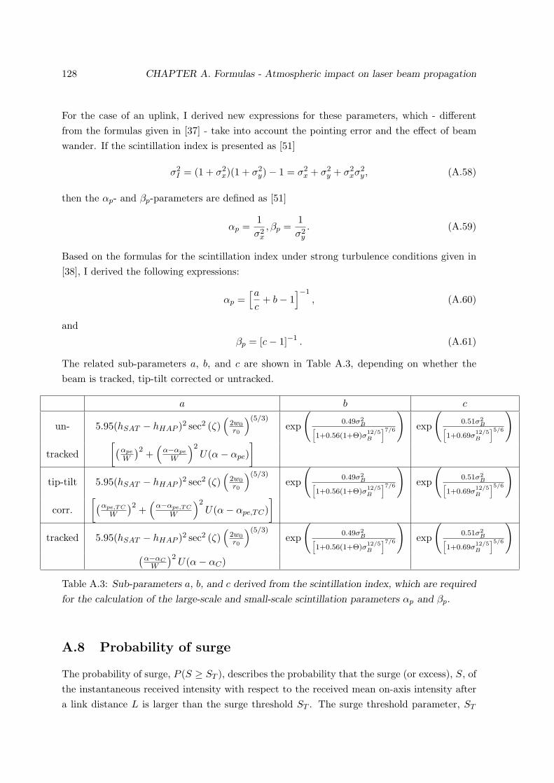
128 CHAPTER A. Formulas - Atmospheric impact on laser beam propagation
For the case of an uplink, I derived new expressions for these parameters, which - differentfrom the formulas given in [37] - take into account the pointing error and the effect of beamwander. If the scintillation index is presented as [51]
σ2I = (1 + σ2
x)(1 + σ2y)− 1 = σ2
x + σ2y + σ2
xσ2y , (A.58)
then the αp- and βp-parameters are defined as [51]
αp =1σ2x
, βp =1σ2y
. (A.59)
Based on the formulas for the scintillation index under strong turbulence conditions given in[38], I derived the following expressions:
αp =[ac
+ b− 1]−1
, (A.60)
and
βp = [c− 1]−1 . (A.61)
The related sub-parameters a, b, and c are shown in Table A.3, depending on whether thebeam is tracked, tip-tilt corrected or untracked.
a b c
un- 5.95(hSAT − hHAP )2 sec2 (ζ)(
2w0r0
)(5/3)exp
(0.49σ2
B[1+0.56(1+Θ)σ
12/5B
]7/6
)exp
(0.51σ2
B[1+0.69σ
12/5B
]5/6
)tracked
[(αpe
W
)2 +(α−αpe
W
)2U(α− αpe)
]tip-tilt 5.95(hSAT − hHAP )2 sec2 (ζ)
(2w0r0
)(5/3)exp
(0.49σ2
B[1+0.56(1+Θ)σ
12/5B
]7/6
)exp
(0.51σ2
B[1+0.69σ
12/5B
]5/6
)corr.
[(αpe,TC
W
)2 +(α−αpe,TC
W
)2U(α− αpe,TC)
]tracked 5.95(hSAT − hHAP )2 sec2 (ζ)
(2w0r0
)(5/3)exp
(0.49σ2
B[1+0.56(1+Θ)σ
12/5B
]7/6
)exp
(0.51σ2
B[1+0.69σ
12/5B
]5/6
)(α−αCW
)2U(α− αC)
Table A.3: Sub-parameters a, b, and c derived from the scintillation index, which are required
for the calculation of the large-scale and small-scale scintillation parameters αp and βp.
A.8 Probability of surge
The probability of surge, P (S ≥ ST ), describes the probability that the surge (or excess), S, ofthe instantaneous received intensity with respect to the received mean on-axis intensity aftera link distance L is larger than the surge threshold ST . The surge threshold parameter, ST

A.9 Expected number of fades per second 129
in [dB], giving the difference between the received on-axis mean irradiance 〈I(0, L)〉 at α = 0and a higher irradiance threshold level IT , is defined as
ST = −10 log(〈I(0, L)〉
IT
). (A.62)
Following the approach for the probability of fade I derived the expression for the probabilityof surge as
P (S ≥ ST ) = P (I ≥ IT ) =∫ ∞IT
p(I)dI = 1−∫ IT
0p(I)dI, (A.63)
which in the case of weak turbulence, i.e. when using the lognormal PDF, leads to
P (S > ST ) = 1− 0.5
1 + erf
0.5σ2I + 2α2L2W−2
eff − 0.23ST√2σ2
I
. (A.64)
A.9 Expected number of fades per second
The expected number of fades per unit time larger than a specified fading threshold level FTare given by [37]
〈n(FT )〉 = ν0 exp
(
0.5σ2I + 2α2L2W−2
eff − 0.23FT)2
−2σ2I
(A.65)
in the case of weak turbulence, i.e. when the scintillation index σ2I is smaller than 1, the
lognormal PDF is used to describe the statistics of the intensity fluctuations. The formularequires the quasi-frequency
ν0 =1
2π
√−BIσ2I
(A.66)
as an input parameter, with
BI = −3.503k13/6µ5dvt(h)2L−1 (hSAT − hHAP )5/6 sec11/6 (ζ) (A.67)
beeing the second derivative of the temporal covariance function for the downlink, and
BI = −3.627k13/6vt(h)2L−1 (hSAT − hHAP )5/6 sec11/6 (ζ)
[µ5u +
µ6uα2L2
3Λ1/6W 2eff
](A.68)
in the uplink. The parameter vt(h) denotes the mean transverse wind speed relative to theoptical beam as given in eqn.(A.26). To calculate the expected number of fades per second inthe case of strong turbulence, based on the gamma-gamma PDF, I used [37]
〈n(FT )〉 =2ν0
√2παpβpσ2
I
Γ(αp)Γ(βp)
(αpβpIT〈I(α,L)〉
)(αp+βp−1)/2
Kαp−βp
(2
√αpβpIT〈I(α,L)〉
), (A.69)
with αp and βp as defined in section A.7.

130 CHAPTER A. Formulas - Atmospheric impact on laser beam propagation
A.10 Mean fade time
The average time at which the fading of the received intensity relative to the mean on-axisintensity is larger than a fading level FT is determined by
〈tf 〉 =P (F > FT )〈n(FT )〉
, (A.70)
where P (F > FT ) is the probability of fade (cf. Section A.7) and 〈n(FT )〉 is the expectednumber of fades per second (cf. Section A.9).
A.11 Beam spread loss
Based on formulas for the beam spot size with and without atmosphere at the receiver in theuplink [41, 37] I calculate the beam spread loss in [dB] as
abs = 20 ∗ log10
[1 +
(DTX
r0
)(5/3)](3/5)
. (A.71)
A similar approach for the downlink leads to
abs = 10 ∗ log10
[1 + 4.35µ2dΛ(5/6)k(7/6)(hSAT − hHAP )(5/6) sec(11/6)(ζ)
]. (A.72)
The evaluation of this formula shows, that the downlink beam spread loss is negligible.
A.12 Coupling efficiency into single-mode fiber
The coupling efficiency η is defined as the ratio of the power carried by the fibre mode F0 andthe power available in the focal plane. It is possible to calculate the coupling efficiency in theaperture plane by the overlap integral
η =∣∣∣∣∫∫
AEF ∗dA
∣∣∣∣2 (A.73)
where E is the input field normalized to its overall power, and F ∗ is the conjugate complexof the fiber mode, backpropagated to the aperture plane A. Because of its circular-symmetry

A.12 Coupling efficiency into single-mode fiber 131
the backpropagated fiber mode can be derived with the help of the Hankel transform:
F (r′) = F−1F0(r) =∫∫
AF0(r) exp [−j2π (νxx+ νyy)]dνxdνy
=∫ ∞
0
∫ 2π
0F0(r) exp [−j2πνrr(cosφ cos θ + sinφ sin θ)]rdrdθ
=∫ ∞
0
∫ 2π
0F0(r) exp [−j2πνrr cos(θ − φ)]rdrdθ
=∫ ∞
0
∫ 2π
0F0(r) exp [−j2πνrr cos(θ)]rdrdθ
=∫ ∞
0F0(r)
[∫ 2π
0exp [−j2πνrr cos(θ)]dθ
]rdr
= 2π∫ ∞
0F0(r)J0 (2πνrr) rdr
= 2π∫ ∞
0F0(r)J0
(2π
r′
λfr
)rdr
= 2π
∫ ρ
0
J0
(U rρ
)J0
(2π r′
λf r)
J0 (U)rdr +
∫ ∞ρ
K0
(W r
ρ
)J0
(2π r′
λf r)
K0 (W )rdr
= 2πρ2
λf
UJ1(U)J0(2π r′
λf ρ)− (2π r′
λf ρ)J0(U)J1(2π r′
λf ρ)
J0(U)(U2 −
(2π r′
λf ρ)2)
+
+ 2πρ2
λf
WK1(W )J0(2π r′
λf ρ)− (2π r′
λf ρ)K0(W )J1(2π r′
λf ρ)
K0(W )(W 2 +
(2π r′
λf ρ)2)
. (A.74)
From this the coupling efficiency can be derived as
η =4χ2
(J2
1 (U)J2
0 (U)+K2
1 (U)K2
0 (U)
)·
·∣∣∣∣∫ χ
0
[UJ1(U)J0(r′)− r′J0(U)J1(r′)
J0(U) (U2 − r′2)+
+WK1(W )J0(r′)− r′K0(W )J1(r′)
K0(W ) (W 2 + r′2)
]exp
(jΦ(r′)
)r′dr′
∣∣∣∣2 , (A.75)
where the phase function Φ(r′) covers any deviations from an ideal plane wavefront. Thedesign parameter
χ = njρ
rA=
2πρaλf
(A.76)
equals χ = 2.05 for optimum coupling conditions at the normalized single-mode cut-off fre-quency V = 2.405 [56]; nj is the first null of the Bessel function, ρ the core radius of thesingle-mode fiber, rA the Airy radius of the Airy field in the focal plane, a the radius of theinput coupling lens, and f the focal length of the lens.

132 CHAPTER A. Formulas - Atmospheric impact on laser beam propagation
In my program the coupling efficiency is calculated via the Strehl ratio [38]
SRuncorr =[1 + (DRX/r0)5/3
]−6/5, (A.77)
for the untracked beam and
SRtilt =
[1 +
(0.983− 0.856
1 + 0.007 (DRX/r0)5/3
)(D/r0)5/3
]−6/5
, (A.78)
in the tip-tilt corrected case.
Appendix B
SimToolPhD - Receiver model
For the calculation of receiver sensitivities when using RZ modulated signals I used the Matlabprogram SimTool, which was developed within our research group and already described indetail in [70, 67, 26, 68]. In the following sections I want to explain the used noise model andcalculation method for the optically preamplified receiver, as well as my modifications for theAPD-based receiver which lead to the actual software version named SimToolPhD+.
B.1 Optically preamplified receiver
For calculating the receiver sensitivity, a quasi-analytical method was applied were signaland noise are represented by their statistical properties, mean and variance. The bit errorprobability is than estimated from these values. The electrical signal after the diode module,specified in terms of voltage, is [26]
s(t) = C∣∣∣(√Gein(t) + nASE
)∗ b(t)
∣∣∣2 ∗ h(t) (B.1)
where ein(t) is the optical input field, G is the preamplifier’s gain, nASE is the stochastic fieldcaused by amplified spontaneous emission from the preamplifier, C the conversion gain of thephoto diode module (given in [V/W]), b(t) and h(t) are the impulse responses1 of the opticaland electrical filter, respectively.
When the noise contributions due to background light (nback) and booster amplifier ASE(nASEb) are taken into account, eqn. (B.1) expands to
s(t) = C∣∣∣(√G (ein(t) + nASEb
√afs + nback
)+ nASE
)∗ b(t)
∣∣∣2 ∗ h(t), (B.2)
where afs accounts for the free space loss between transmitter and receiver.As discussed in Section 3.3.2.1, three effects contribute to the electrical signal’s variance:
shot noise (according to signal, dark current, preamplifier ASE, booster ASE, and background
1The operator ∗ represents a convolution: (x ∗ y)(t) =∞∫−∞
x(τ)y(t− τ)dτ .
133

134 CHAPTER B. SimToolPhD - Receiver model
noise), beat noise (between signal, preamplifier ASE, booster ASE, and background noise),and thermal noise of the receiver electronics, leading to a noise variance of
σ2s(t) = σ2
shot,s(t) + σ2shot,d(t) + σ2
shot,ASE(t) + σ2shot,ASEb(t) + σ2
shot,back(t)
= +σ2s-ASE(t) + σ2
s-ASEb(t) + σ2s-back(t) + σ2
ASE-ASEb(t) + σ2ASE-back(t)
= +σ2ASE-ASE(t) + σ2
ASEb-ASEb(t) + σ2back-back(t)
= +σ2elec(t). (B.3)
The relevant noise term contributions2, as illustrated in Fig.3.22, are
• noise originating from beating between signal and ASE [67]
σ2s-ASE(t) = 2C2NASERe
∞∫∫−∞
ef (τ)e?f (τ)rb(τ − τ)h(t− τ)h(t− τ)dτdτ, (B.4)
where NASE is the power spectral density of the amplified spontaneous emission ofthe preamplifier (cf. eqn. (3.16)), ef (t) =
√G(ein ∗ b)(t) is the optically amplified and
filtered field, and rb(t) is the optical filter’s autocorrelation function corresponding tothe definition
rb(t) =∫ ∞−∞
b(τ)b?(τ − t)dτ, (B.5)
• the beating of the preamplifier ASE with itself [67],
σ2ASE-ASE = 2C2N2
ASE
∞∫−∞
|rb(τ)|2rh(τ)dτ, (B.6)
and
• electronic noiseσ2
elec = N2elR
2TBe . (B.7)
defined by the diode module’s noise equivalent current (Nel), given in [A/√
Hz], withBe the electrical filter bandwidth and RT being the resistance that converts the outputcurrent of the photodiode into a voltage.
B.2 APD-based receiver
For the APD-based receiver, I expressed the electrical signal after the diode module, specifiedin terms of voltage, as
s(t) = CM∣∣(ein(t) + nASEb
√afs + nback
)∗ b(t)
∣∣2 ∗ h(t), (B.8)
2For the calculation of the beat noise terms an advanced Gaussian model is used [70, 26], where the exact
variance is calculated, taking into account the actual filter transfer functions.

B.3 Receiver sensitivity 135
where ein(t) is the optical input field, M is the APD gain, nASEb is the stochastic field causedby amplified spontaneous emission from the booster amplifier, nb is the stochastic field causedby background noise, C the conversion gain of the photodiode module (given in [V/W]), b(t)and h(t) are the impulse responses of the optical and electrical filter, respectively.
Three effects contribute to the electrical signal’s variance: shot noise (according to signal,dark current, booster ASE, and background noise), beat noise (between signal, booster ASE,and background noise), and thermal noise of the receiver electronics, leading to
σ2s(t) = σ2
shot,s(t) + σ2shot,d(t) + σ2
shot,ASEb(t) + σ2shot,back(t)
= +σ2s-ASEb(t) + σ2
s-back(t) + σ2ASEb-ASEb(t) + σ2
back-back(t)
= +σ2elec(t). (B.9)
The relevant noise term contributions, as illustrated in Fig.3.25, are
• the shot noise according to signal
σ2shot,s = SR2
TM2Fapde(|(ein ∗ b)(t)|2 ∗ h2(t)), (B.10)
where S in [A/W] is the photodiode’s responsivity, RT is the resistance that convertsthe output current of the photodiode into a voltage, Fapd is the APD noise figure, ande = 1.602 · 10−19 As is the elementary charge of an electron,
• the dark current shot noise
σ2shot,d = 2eMIDFapdBeR
2T , (B.11)
and
• the noise of the receiver electronics
σ2elec = N2
elR2TBe (B.12)
determined by the diode module’s noise equivalent current (Nel), given in [A/√
Hz].
B.3 Receiver sensitivity
With the expressions for signal (eqn.(B.2) and eqn.(B.8)) and noise (eqn.(B.3) and eqn.(B.9))as denoted in the previous appendices, the BEP at a sampling time Ts and for a decisionthreshold Sth is [115]
BEP(Ts, Sth) =1
2n − 1
∑k0
12
erfc[Sth − s(Ts + k0Tb)√
2σs(Ts + k0Tb)
]+∑k1
12
erfc[s(Ts + k1Tb)− Sth√
2σs(Ts + k1Tb)
],
(B.13)

136 CHAPTER B. SimToolPhD - Receiver model
where the indices k0 and k1 are used to distinguish between 2n−1 − 1 “0”-bits and 2n−1 “1”-bits of the PN sequence3. The receiver sensitivity ns then is defined as the required averagenumber of photons per bit at the optical amplifier input to achieve a BEP = 10−9.
3To take ISI into consideration with sufficient accuracy, it is necessary that the length of the bit sequence is
at least 27−1 [116].

Appendix C
Datasheets
137
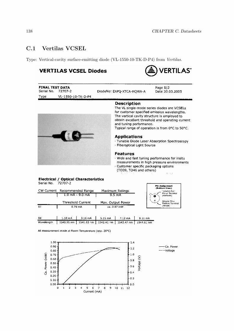
138 CHAPTER C. Datasheets
C.1 Vertilas VCSEL
Type: Vertical-cavity surface-emitting diode (VL-1550-10-TK-D-P4) from Vertilas.

C.1 Vertilas VCSEL 139

140 CHAPTER C. Datasheets
C.2 RayCan VCSEL
Type: Vertical-cavity surface-emitting diode (RT3xxx1-F) from RayCan.

C.2 RayCan VCSEL 141

142 CHAPTER C. Datasheets

C.3 DFB/EAM laser module 143
C.3 DFB/EAM laser module
Type: DFB/EAM laser module for 10 Gbit/s (PGT 202 04) from Ericsson.

144 CHAPTER C. Datasheets
C.4 Pin-receiver
Type: R2860C Digital Receiver OC-192/STM-64 from Lucent Technologies.

C.5 APD-receiver 145
C.5 APD-receiver
Type: AT10XGC 10.709 Gbit/s surface mount coplanar APD receiver from Bookham.
Operating Characteristics
Case Temperature = 25°C unless otherwise specified
www.bookham.com Thinking optical solutionswww.bookham.com Thinking optical solutions
Parameter Symbol Measurement Min Typ Max UnitConditions
Optical sensitivity BOL1, 2 Sens 231-1 PRBS -28.5 -27.0 dBmBER<10-12
Voptimal = VM10
Sensitivity penalty EOL 231-1 PRBS 0.75 1.0 dBover temperature1, 2 BER<10-12
Voptimal = VM10
T=0 to +85°C
Deviation from linear phase DC - 6GHz -10 +10 °
High frequency -3dB corner fH VAPD=VM10 8 9 GHzSmall signal
Low frequency -3dB corner fL 40 kHz
Transimpedance gain3, 4, 5 TZ Small signal 2.3 4.0 5.7 kΩ
Maximum output voltage6 VOUT Peak-to-peak 165 mV
Return loss S22 DC to 6.0GHz -8 dB
Optical overload2 PSAT 2^23-1 PRBS -3 -1 dBmVAPD=VM3
BER<10-12
APD breakdown voltage Vbr T=25°C 20 40 VIAPD=10µA
APD breakdown voltage TVbr 0.030 0.061 V/°Ctemperature coefficient
Dark current Id At 90% of Vbr 100 nA
Amplifier bias current Icc 55 73 mA
Input current for output limiting IIn lim Peak-to-peak 80 uA
Transimpedance amp VTZA 3.3 Vsupply voltage
Thermistor resistance RTH T=25°C 10 kΩ
Notes:1. Optical Wavelength between 1525-1575nm. Data to 1610nm available on request.2. Measured with 9.95Gb/s, extinction ratio > 12dB, Q factor > 30, 50% crossing level, 1550nm.3. Load impedance is 50Ω AC-coupled4. Excludes APD responsivity5. Differential6. Single ended

146 CHAPTER C. Datasheets
www.bookham.com Thinking optical solutionswww.bookham.com Thinking optical solutions
Pin Out
Pin # Symbol Function Pin # Symbol Function
1 NC Case ground 10 Out_P Positive RF data output
2 VAPD APD bias voltage 11 GND Case RF ground
3 NC No connection 12 GND Case ground
4 NC No connection 13 NC No connection
5 NC No connection 14 VCC Amplifier supply (+3.3V)
6 GND Case ground 15 NC No connection
7 GND Case RF ground 16 RTH Thermistor
8 Out_N Negative RF data output 17 GND Case ground
9 GND Case ground
Absolute Maximum Ratings
The table below provides maximum and/or minimum values of critical parameters which will not permanently damage thedevice, but for which the operating specification may not hold.
Parameter Symbol Min Max Unit
Amplifier bias voltage VCC -0.7 5.0 V
Operating temperature1 Top 0 +85 °C
Storage temperature2 Tstg -40 +85 °C
Input photocurrent3 IPD 3 mA
APD bias voltage VAPD 0 Vbr V
Fiber bend radius 20 mm
Notes:1. The operating temperature is defined as the temperature of the module case.2. The rating is referred to the ambient temperature.3. VAPD ≥ VM3. Although implementation of a current limit is intuitive, it is not recommended as biasing below thespecified M = 3 voltage in the presence of a high optical power has been shown to cause device damage.
Class 2 ESD precautions must be observed when handling these devices.
Deliverable Data
VM3 and Vbr are provided on the fiber tag for each device.

Appendix D
Abbreviations, constants, and
symbols
D.1 List of abbreviations
APD avalanche photo diodeARQ automatic repeat requestARTEMIS advanced relay and technology mission satelliteASE amplified spontaneous emissionBEP bit error probabilityBER bit error ratioBTJ buried tunnel junctionCCD charge-coupled deviceCDF cumulative distribution functionCMOS complementary metal oxide semiconductorCW continues waveDBR distributed Bragg reflectorDD direct detectionDFB distributed feed-backDI delay interferometerDL diffraction limitDLR Deutsches Zentrum fur Luft- und RaumfahrtDPSK differential phase shift keyingDSL digital subscriber lineDVB digital video broadcastingDVD digital versatile discDWDM dense wavelength division multiplexingEAM electro-absorption modulator
147

148 CHAPTER D. Abbreviations, constants, and symbols
EDFA Erbium-doped fiber amplifierEFEC enhanced forward error correctionEPR Einstein, Podolsky, and RosenESA European Space AgencyFBG fiber Bragg gratingFEC forward error correctionFOV field of viewFP Fabry-PerotGEO geostationary orbitGPS global positioning systemHAA high altitude airshipHALE high altitude long enduranceHAP high altitude platformIM intensity modulationISI intersymbol interferenceISS International Space StationITU International Telecommunication UnionJAXA Japan Aerospace Exploration AgencyJPL jet Propulsion LaboratoryKARI Korea Aerospace Research InstituteLCT laser communication terminalLEO low Earth orbitLOLA liaison optique laser aeroporteeLOS line of sightLUCE laser utilizing communications equipmentMZM Mach-Zehnder modulatorNASA National Aeronautics and Space AdministrationNICT National Institute of Information and Communications TechnologyNRZ non-return-to-zeroOICETS optical inter-orbit communications engineering test satelliteOGS optical ground stationOOK on/off keyingOPALE optical payload for inter-satellite link experimentOSA optical spectrum analyzerPASTEL passenger telecomPAT pointing, acquisition, and trackingPBS polarization beam splitterPDF probability density functionPhD philosophiae doctor

D.2 List of physical and mathematical constants 149
PM phase modulatorPOLSK polarization shift keyingPPM pulse position modulationPRBS pseudo random bit sequencePSK phase shift keyingQPD quadrant photodiodeRF radio-frequencyRMS root mean squareRS Reed SolomonRX receiverRZ return-to-zeroSAT satelliteSFEC standard forward error correctionSILEX semi-conductor laser inter-satellite link experimentSMA sub miniature version A connectorSMF single-mode fiberSOP state of polarizationSPOT-4 satellite pour l‘observation de la terre 4TX transmitterUAV unmanned aerial vehicleVCSEL vertical-cavity surface-emitting laserVNA vector network analyzer
D.2 List of physical and mathematical constants
c = 2.9979 · 108 m/s free space light velocitye = 1.602 · 10−19 As elementary chargee = 2.7183 Euler’s constanth = 6.6262 · 10−34 Js Planck’s constantj =√−1 imaginary unit
k = 1.3807 · 10−23 J/K Boltzmann’s constantπ = 3.1416 pi
D.3 List of Latin symbols
aatm loss due to atmospheric absorption and scatteringabs loss due to beam spreadach,lt “long-term” channel loss due to fadingach,st “short-term” channel loss due to fadingach,t “short-term” channel loss due to fading at certain mean fade time
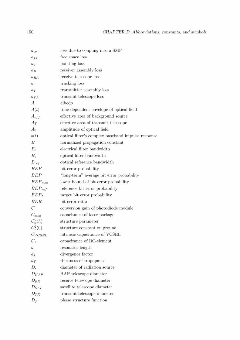
150 CHAPTER D. Abbreviations, constants, and symbols
aco loss due to coupling into a SMFafs free space lossap pointing lossaR receiver assembly lossaRA receive telescope lossat tracking lossaT transmitter assembly lossaTA transmit telescope lossA albedoA(t) time dependent envelope of optical fieldAeff effective area of background sourceAT effective area of transmit telescopeA0 amplitude of optical fieldb(t) optical filter’s complex baseband impulse responseB normalized propagation constantBe electrical filter bandwidthBo optical filter bandwidthBref optical reference bandwidthBEP bit error probabilityBEP “long-term” average bit error probabilityBEPmin lower bound of bit error probabilityBEP ref reference bit error probabilityBEP t target bit error probabilityBER bit error ratioC conversion gain of photodiode moduleCcase capacitance of laser packageC2n(h) structure parameter
C2n(0) structure constant on ground
CV CSEL intrinsic capacitance of VCSELC1 capacitance of RC-elementd resonator lengthdf divergence factordT thickness of tropopauseDs diameter of radiation sourceDHAP HAP telescope diameterDRX receive telescope diameterDSAT satellite telescope diameterDTX transmit telescope diameterDϕ phase structure function

D.3 List of Latin symbols 151
DC duty cycleef (t) optically amplified and filtered fieldE optical fieldE1 optical energy for ‘1’ bitEin optical input fieldf focal lengthfc center frequencyF fading depthF preamplifier noise figureFξ cumulative distribution functionFag equivalent noise figureFapd APD noise figureFb booster amplifier noise figureFT fading thresholdF (r′) optical field of fundamental fiber mode backpropagated to aperture planeF0(r) optical field of fundamental fiber modegch,FEC FEC coding gainG preamplifier gainGb booster amplifier gainGR receive antenna gainGT transmit antenna gainG(ω) spectral filterh height above groundh(t) impulse response of photo diode modulehHAP altitude of high-altitude-platform, height above groundhSAT altitude of a satellite, height above groundhT height of tropopauseHrefl reflected spectral background irradianceHself self-emitted spectral background irradianceI intensityI currentIbias laser bias currentId dark currentImod peak-to-peak laser modulation currentIT intensity threshold levelIth threshold current〈I(0, L)〉 on-axis mean intensity〈I(r, L)〉 off-axis mean intensityJ0(ξ) Bessel function of the first kind and of zero order

152 CHAPTER D. Abbreviations, constants, and symbols
k optical wave numberK number of data symbolsK0(ξ) modified Bessel function of the second kind and of zero orderl1 distanceL transmission distanceLbond inductance of bonding wiresLwire inductance of connection wiresm number of spatial modesM magnitudeM APD multiplication factorM number of bitsn refractive index〈n(F > FT )〉 expected number of fadesnq quantum limit of receiver sensitivityns receiver sensitivityN number of symbols per codewordNASE ASE noise power spectral densityNb noise power density from booster amplifier ASENback background noise power densityNel electrical noise power densityN0 noise power spectral densityOSNR optical signal-to-noise ratiop(ξ) probability density functionpBEP probability for a certain BEPpFEC probability for a certain effective coding gainpm power marginP average optical powerP (F > FT ) probability of fadeP (S > ST ) probability of surgePASEb average of the optically filtered transmitter booster’s ASEPback average of the optically filtered background noisePref reference optical power to achieve BEPrefPR received powerPt target optical power to achieve BEPtPT transmitted powerP0 optical power during a logical ‘0’P1 optical power during a logical ‘1’q number of bits per symbolr radial coordinate

D.3 List of Latin symbols 153
rb(t) optical filter’s autocorrelation functionrd differential resistancerEarth radius of Earthrh(t) electrical filter’s autocorrelation functionr0 Fried parameterR data rateR(z) phase front curvatureR(λ) spectral radianceRMSλ RMS phasefront perturbation in fractions of the wavelengthRs symbol rateRT transimpedanceR1 resistance of RC-elements(t) mean of the electrical signal after the diode moduleS surgeS detector sensitivity (responsivity)S(τ,Ω) sonogramSRX receiver sensitivityST surge thresholdSRmar Strehl ratio, Marechal approximationSRtilt Strehl ratio, tip-tilt corrected beamSRuncorr Strehl ratio, untracked beamt timet bit error correction capabilityte number of erroneous bits〈tf 〉 mean fade timetF fall timetR rise timett target number of erroneous bitsT temperatureT correctable symbol errors per codewordTb bit durationTeff effective temperatureTp pulse durationTse temperature of self-emitting sourceT0 temperature constant (semiconductor laser)U voltagevHAP HAP moving speedvmov velocity term due to HAP movementvn HAP speed component normal to LOS

154 CHAPTER D. Abbreviations, constants, and symbols
vRMS rms wind speedvt mean wind speed relative to optical beamvt,rms transverse rms wind speedvT wind speed at tropopausevwind wind speed on groundV normalized frequencywin 1/e2 (intensity) radius of incoming beamwout 1/e2 (intensity) radius of outgoing beamW beam radiusWDL diffraction limited beam radiusWeff effective beam radiusx transverse x-coordinatey transverse y-coordinatez longitudinal z-coordinate
D.4 List of Greek symbols
α angular pointing errorα roll-off factorαc linewidth enhancement factor (chirp parameter)αn normalized angular pointing errorαT beam truncationβimb amplitude imbalance∆f frequency difference∆τ delay imbalance∆ϕ phase differenceγ elevation angleγoff offset angle of polarization basisγorth non-orthogonality of polarization basisγq sensitivity penaltyε extinction ratio MZMζ zenith angleζex extinction ratioη power coupling efficiency into SMFηmax maximum power coupling efficiency into SMFηsl slope efficiencyθ half-angle beam divergenceθDL diffraction limited divergence angleθeff effective divergence angle

D.4 List of Greek symbols 155
θFOV planar of the receiver’s field of viewκ geometry constant of semiconductor laserλ wavelengthµϕ mean value of phase variationν0 quasi-frequencyρ core radius of single-mode fiberρch transverse correlation widthρd distance between two points on phasefrontσB Rytov varianceσ2I scintillation indexσ2s(t) variance of electrical signal at input of decision gateσ2
shot,ASEb(t) variance according to booster ASE shot noiseσ2
shot,back(t) variance according to background shot noiseσ2
shot,d(t) variance according to dark current shot noiseσ2
shot,s(t) variance according to signal-shot noiseσ2
shot,ASE(t) variance according to ASE-shot noiseσ2
s-ASE(t) variance according to signal-ASE beat noiseσ2
s-ASEb(t) variance according to signal - booster ASE beat noiseσ2
s-back(t) variance according to signal - background beat noiseσ2
ASE-ASE(t) variance according to ASE-ASE beat noiseσ2
ASEb-ASEb(t) variance according to booster ASE - booster ASE beat noiseσ2
back-back(t) variance according to background-background beat noiseσ2
elec(t) variance according to electronic noiseσ2ϕ phase varianceτ time constantτch correlation timeϕ0 phase of optical fieldφ(t) time dependent phaseΦ(r′) phase functionχ design parameter for calculation of coupling efficiencyω angular frequencyωs slew rate of optical beamω0 carrier frequencyΩs solid angle subtended by the source at the receiverΩFOV solid angle of the receiver’s field of viewΩ filter frequency offset

156 CHAPTER D. Abbreviations, constants, and symbols

Bibliography
[1] H. Potocnik, Das Problem der Befahrung des Weltraums - Der Raketen-Motor, 1st ed.Berlin: Richard Carl Schmidt & Co., 1929.
[2] COST 297. (2007, February) HAPCOS - high altitude platforms for communicationsand other services. [Online]. Available: www.hapcos.org
[3] T. C. Tozer and D. Grace, “Broadband service delivery from high altitude platforms,”in Communicate 2000 Online Conference, London, UK, October 2000.
[4] D. Giggenbach, R. Purvinskis, M. Werner, and M. Holzbock, “Stratospheric optical inter-platform links for high altitude platforms,” in 20th AIAA International CommunicationsSatellite Systems Conference and Exhibit, Montreal, Canada. Reston: AIAA, 2002, p.1910.
[5] R. A. Fesen, “A high-altitude station-keeping astronomical platform,” Proc. of the SPIE,vol. 6267, p. 62670T, 2006.
[6] StratXX. (2007, February). [Online]. Available: www.stratxx.com
[7] US Air Force. (2005, October). [Online]. Available: www.af.mil/factsheets/factsheet.asp?fsID=175
[8] NASA. (2006, July). [Online]. Available: www.nasa.gov/centers/dryden/history/pastprojects/Helios/index.html
[9] AeroVironment. (2007, February). [Online]. Available: www.avinc.com/uas dev projectdetail.php?id=115
[10] QinetiQ. (2007, February). [Online]. Available: www.qinetiq.com/home/aerospace/defence air/uav.html
[11] USE HAAS. (2006, October) High altitude aircraft and airships. [Online]. Available:www.usehaas.org
[12] M. Toyoshima, “Trends in satellite communications and the role of optical free-spacecommunications,” Journal of Optical Networking, vol. 4, pp. 300–311, 2005.
157

158 BIBLIOGRAPHY
[13] H. Hemmati, Deep Space Optical Communications. New York: John Wiley & Sons,Inc., 2006.
[14] W. R. Leeb, “Optische Nachrichtentechnik,” Lecture Notes, Institut fur Nachrichten-technik und Hochfrequenztechnik, TU Wien, 2007.
[15] S. G. Lambert and W. L. Casey, Laser Communications in Space. Artech House, 1995.
[16] J. Horwath, M. Knapek, B. Epple, M. Brechtelsbauer, and B. Wilkerson, “Broadbandbackhaul communication for stratospheric platforms: The stratospheric optical payloadexperiment (STROPEX),” in Proc. of the SPIE, Vol. 6304, Free-Space Laser Commu-nications VI, San Diego, USA. SPIE, September 2006, p. 63041N.
[17] M. Antonini, E. Cianca, A. DeLuise, M. Pratesi, and M. Ruggieri, “Stratospheric relay:potentialities of new satellite-high altitude platforms integrated scenarios,” in Proceed-ings of IEEE Aerospace Conference, March 2003, pp. 1211–1219.
[18] G. Planche and V. Chorvalli, “SILEX in-orbit performances,” in Proc. of the 5th Inter-national Conference on Space Optics (ICSO 2004),Toulouse, France. Noordwijk: ESA,April 2004, pp. 403–410.
[19] M. Toyoshima, S. Yamakawa, T. Yamawaki, K. Arai, M. Reyes-Garcıa-Talavera,A. Alonso, Z. Sodnik, and B. Demelenne, “Long-term statistics of laser beam propagationin an optical ground-to-geostationary satellite communication link,” IEEE Transactionson Antennas and Propagation, vol. 53, no. 2, pp. 842–850, 2005.
[20] G. Baister and P. V. Gatenby, “Pointing, acquisition, and tracking for optical space com-munications,” IEEE Electronics & Communication Engineering Journal, vol. 6, no. 6,pp. 271–280, 1994.
[21] T. Jono, Y. Takayama, K. Ohinata, N. Kura, Y. Koyama, K. Arai, K. Shiratama, Z. Sod-nik, A. Bird, and B. Demelenne, “Demonstrations of ARTEMIS-OICETS inter-satellitelaser communications,” in 24th AIAA International Communications Satellite SystemsConference, San Diego, USA. Reston: AIAA, 2006, p. 5461.
[22] R. Lange and B. Smutny, “Homodyne BPSK-based optical inter-satellite communicationlinks,” Proceedings of the SPIE, Free-Space Laser Communication Technologies XIX andAtmospheric Propagation of Electromagnetic Waves, vol. 6457, pp. 645 703–1...645 703–9,2007.
[23] CAPANINA Consortium. (2007, February) CAPANINA - stratospheric broadband.[Online]. Available: www.capanina.org
[24] ESA. (2006, December) Another world first for ARTEMIS: a laser link with an aircraft.[Online]. Available: www.esa.int/esaTE/SEMN6HQJNVE index 0.html

BIBLIOGRAPHY 159
[25] M. Toyoshima, “Lightwave propagation in the presence of random turbulent media andpointing jitter in optical space communications,” Doctoral Thesis, University of Tokyo,Tokyo, Japan, 2003.
[26] M. Pfennigbauer, “Design of optical space-to-ground links for the International SpaceStation,” Doctoral Thesis, Institut fur Nachrichtentechnik und Hochfrequenztechnik, TUWien, 2004.
[27] A. Colozza and J. L. Dolce. (2005, February) High-altitude, long-endurance airships forcoastal surveillance. [Online]. Available: gltrs.grc.nasa.gov
[28] B. J. Klein and J. J. Degnan, “Optical antenna gain. 1: Transmitting antennas,” AppliedOptics, vol. 13, no. 9, pp. 2134–2141, 1974.
[29] P. J. Winzer, A. Kalmar, and W. R. Leeb, “Intersatellite laser communications at 1.5µm:Chances and problems,” Institut fur Nachrichtentechnik und Hochfrequenztechnik, TUWien,” European Space Agency Contract Report, Contract No. 11846/96/NL/SB(SC),1998.
[30] W. R. Leeb, “Technical Note 2: 1550 nm Laser Communication Terminal AdaptationStudy,” Institut fur Nachrichtentechnik und Hochfrequenztechnik,” European SpaceAgency Contract Report, ESTEC, Contract No. 19393/05/NL/SFe, 2006.
[31] G. P. Agrawal, Fiber-optic Communication Systems, 3rd ed. New York: John Wiley &Sons, Inc., 2002.
[32] P. Wysocki, T. Wood, A. Grant, D. Holocomb, K. Chang, M. Santo, L. Braun, andG. Johnson, “High reliability of 49 dB gain, 13 W PM fiber amplifier at 1550 nm with30 dB PER and record efficiency,” in Proceedings of Optical Fibers CommunicationConference (OFC), Anaheim, USA. OSA, March 2006, p. PDP17.
[33] I. Kaminow and T. Li, Optical Fiber Telecommunications, 4th ed. New York: AcademicPress, 2002.
[34] W. K. Pratt, Laser Communication Systems, 1st ed. New York: John Wiley & Sons,Inc., 1969.
[35] J. Alwan. (2007, August) Eye safety and wireless optical networks (WONs). [Online].Available: www.freespaceoptics.com/AirFiber-FSO-Eye-Safety.pdf
[36] K. Kudielka, W. M. Neubert, A. Scholtz, and W. R. Leeb, “Adaptive optical multi-aperture receive antenna for coherent intersatellite communication,” Proceedings of theSPIE, Space Instrumentation and Spacecraft Optics, vol. 2210, pp. 61–70, 1994.
[37] L. C. Andrews and R. L. Phillips, Laser Beam Propagation through Random Media,2nd ed. SPIE - The International Society for Optical Engineering, 2005.

160 BIBLIOGRAPHY
[38] L. C. Andrews, R. L. Phillips, R. J. Sasiela, and R. R. Parenti, “Strehl ratio and scin-tillation theory for uplink Gaussian-beam waves: beam wander effects,” SPIE OpticalEngineering, vol. 45, no. 7, pp. 76 001–1..76 001–12, 2006.
[39] B. Epple, “Development and implementation of a pointing, acquisition and trackingsystem for optical free-space communication systems on high altitude platforms,” MasterThesis, Institut fur Informatik, Ludwig-Maximilians-Universitat Munchen, 2005.
[40] L. C. Andrews, Field Guide to Atmospheric Optics. SPIE - The International Societyfor Optical Engineering, 2004.
[41] H. Kogelnik and T. Li, “Laser beams and resonators,” Proceedings of the IEEE, vol. 54,no. 10, pp. 1312–1329, 1966.
[42] R. E. Hufnagel, “Variations of atmospheric turbulence,” in Digest of Technical Papers,Optical Propagation through Turbulence: Topical Meeting; Colorado, Boulder, July 1974,pp. Wa1–1...Wa1–4.
[43] J. Horwath, F. David, M. Knapek, and N. Perlot, “Coherent transmission feasibilityanalysis,” Proceedings of the SPIE, Free-Space Laser Communication Technologies XVII,vol. 5712, pp. 13–23, 2005.
[44] T. C. Tozer and D. Grace, “High-altitude platforms for wireless communications,” IEEElectronics & Communication Engineering Journal, vol. 13, no. 3, pp. 127–137, 2001.
[45] E. H. Teets and P. O. Harvey, “Comparison of three wind measuring systems for flighttest,” in 9th Conference on Aviation, Range, and Aerospace Meteorology, Orlando, USA,2000, pp. 177–181.
[46] D. L. Fried, “Statistics of a geometric representation of wavefront distortion,” Journalof the Optical Society of America, vol. 55, pp. 1427–1435, 1965.
[47] R. J. Noll, “Zernike polynomials and atmospheric turbulence,” Journal of the OpticalSociety of America, vol. 66, no. 3, pp. 207–211, 1976.
[48] T. G. Bifano, J. Perreault, R. K. Mali, and M. N. Horenstein, “Microelectromechanicaldeformable mirrors,” IEEE Journal of Selected Topics in Quantum Electronics, vol. 5,no. 1, pp. 83–89, 1999.
[49] M. Reyes, A. Alonso, S. Chueca, J. J. Fuensalida, A. Comeron, V. F. Dios, A. Rodriguez,J. A. Rubio, and Z. Sodnik, “Propagation statistics of ground-satellite optical linkswith different turbulence conditions,” Proceedings of the SPIE, Optics in AtmosphericPropagation and Adaptive Systems VII, vol. 5572, pp. 211–222, 2004.
[50] J. H. Churnside, “Aperture averaging of optical scintillations in the turbulent atmo-sphere,” Applied Optics, vol. 30, no. 15, pp. 1982–1994, 1991.

BIBLIOGRAPHY 161
[51] M. A. Al-Habash, L. C. Andrews, and R. L. Phillips, “Mathematical model for theirradiance probability density function of a laser beam propagating through turbulentmedia,” Optical Engineering, vol. 40, no. 8, pp. 1554–1562, 2001.
[52] R. Parenti, R. J. Sasiela, L. C. Andrews, and R. L. Phillips, “Modeling of the PDF forthe irradiance of an uplink beam in the presence of beam wander,” Proceedings of theSPIE, vol. 6215, pp. 621 508–1...621 508–13, 2006.
[53] F. Stromqvist-Vetelino, J. Recolons, L. C. Andrews, C. Young, B. Clare, K. Corbett,and K. Grant, “PDF models of the irradiance fluctuations in Gaussian beam waves,”Proceedings of the SPIE, vol. 6215, pp. 62 150A–1...62 150A–9, 2006.
[54] L. C. Andrews and R. L. Phillips, Laser Beam Propagation through Random Media,1st ed. SPIE - The International Society for Optical Engineering, 1998.
[55] R. K. Tyson, “Adaptive optics and ground-to-space laser communications,” Appl. Opt.,vol. 35, pp. 3640–3646, 1996.
[56] O. Wallner, “Modal filtering of optical waves,” Doctoral Thesis, Institut fur Nachricht-entechnik und Hochfrequenztechnik, TU Wien, 2004.
[57] S. M. Watson, C. J. Subich, and K. D. Ridley, “Phase structure function of random wavefields,” Optics Communications, vol. 270, pp. 105–115, 2007.
[58] C. Ruilier, “A study of degraded light coupling into single-mode fibers,” Proceedings ofthe SPIE, Astronomical Interferometry, vol. 3350, pp. 319–329, 1998.
[59] T. A. Brummelaar and W. G. Bagnuolo, “Strehl ratio and visibility in long baselinestellar interferometry,” Optics Letters, vol. 20, pp. 521–523, 1995.
[60] R. M. Goody and Y. L. Yung, Atmospheric radiation: theoretical basis, 2nd ed. OxfordUniversity Press, 1989.
[61] W. R. Leeb, “Degradation of signal to noise ratio in optical free space data links due tobackground illumination,” Applied Optics, vol. 28, no. 15, pp. 3443–3449, 1989.
[62] R. C. Ramsey, “Spectral irradiance from stars and planets, above the atmosphere, from0.1 to 100.0 microns,” Applied Optics, vol. 1, no. 4, pp. 465–471, 1962.
[63] A. Cox, Allen’s Astrophysical Quantities, 4th ed. Berlin: Springer Verlag, 2000.
[64] B. J. Anderson and R. E. Smith, “Natural Orbital Environment Guidelines for Use inAerospace Vehicle Development,” NASA,” Technical Manual 4527, 1994.
[65] B. Keidel, “Auslegung und simulation von hochfliegenden, dauerhaft stationierbarensolardrohnen,” Doctoral Thesis, Technical University Munich, 2000.

162 BIBLIOGRAPHY
[66] P. J. Winzer, “Optical transmitters, receivers, and noise,” Wiley Encyclopedia ofTelecommunications, J.G.Proakis (ed.), pp. 1824–1840, 2002.
[67] P. J. Winzer, M. Pfennigbauer, M. M. Strasser, and W. R. Leeb, “Optimum filterbandwidths for optically preamplified NRZ and RZ receivers,” J. Lightwave Technol-ogy, vol. 19, no. 9, pp. 1263–1273, 2001.
[68] F. Fidler, “Performance enhancement in wdm systems,” Master Thesis, Institut furNachrichtentechnik und Hochfrequenztechnik, TU Wien, 2004.
[69] D. O. Caplan, “High-performance free-space laser communications and future trends,”in Optical Amplifiers and Their Applications, 2005, p. TuB1.
[70] M. Pfennigbauer, “Simulation von Empfangern fur optisch vorverstarkte Return-to-ZeroSignale,” Diploma Thesis, Institut fur Nachrichtentechnik und Hochfrequenztechnik, TUWien, 2000.
[71] P. J. Winzer and A. Kalmar, “Sensitivity enhancement of optical receivers by impulsivecoding,” IEEE Journal of Lightwave Technology, vol. 17, no. 2, pp. 171–177, 1999.
[72] D. O. Caplan and W. A. Atia, “A quantum-limited optically-matched communicationlink,” in Proc. OFC’01, Opitcal Fiber Communication Conference, 2001.
[73] M. Pfennigbauer, M. M. Strasser, M. Pauer, and P. J. Winzer, “Dependence of opticallypreamplified receiver sensitivity on optical and electrical filter bandwidths – measure-ment and simulation,” IEEE Photonics Technology Letters, vol. 14, no. 6, pp. 831–833,2002.
[74] G. Jacobsen, Noise in digital optical transmission systems. Artech House, 1994.
[75] G. Jacobsen, “Performance of preamplified direct detection systems under influence ofreceiver noise,” IEEE Photonics Technology Letters, vol. 6, no. 12, pp. 1488–1490, 1994.
[76] Advanced Optics Solutions (AOS Fiber). (2006, February). [Online]. Available:www.aos-fiber.com
[77] A. H. Gnauck and P. J. Winzer, “Optical phase-shift-keyed transmission,” IEEE Journalof Lightwave Technology, vol. 23, no. 1, pp. 115–130, 2005.
[78] M. Pauer, “Return-to-zero coding in optical intersatellite links,” Doctoral Thesis, Insti-tut fur Nachrichtentechnik und Hochfrequenztechnik, TU Wien, 2003.
[79] J. J. Lepley, J. G. Ellison, S. G. Edirisinghe, A. S. Siddiqui, and S. D. Walker, “Ex-cess penalty impairments of polarization shift keying transmission format in presence ofpolarization mode dispersion,” Electronic Letters, vol. 36, no. 8, pp. 736–737, 2000.

BIBLIOGRAPHY 163
[80] E. S. Hu, Y. Hsueh, K. Shimizu, K. K. Y. Wong, N. Kikuchi, M. E. Marhic, and L. G.Kazovsky, “4-level direct-detection polarization shift-keying (DD-POLSK) system withphase modulators,” in Proc. OFC’03, Opitcal Fiber Communication Conference, 2003.
[81] S. Benedetto, A. Djupsjobacka, B. Lagerstrom, R. Paoletti, P. Poggiolini, and G. Mijic,“Multilevel polarization modulation using a specifically designed LiNb03 device,” IEEEPhotonics Technology Letter, vol. 6, no. 8, pp. 949–951, 1994.
[82] S. Benedetto, R. Gaudion, and P. Poggiolini, “Direct detection of optical digital trans-mission based on polarization shift keying modulation,” IEEE Journal on Selected Areasin Communications, vol. 13, no. 3, pp. 531–542, 1995.
[83] M. Ott, “Validation of commercial fiber optic components for aerospace environments,”in Conference on Smart Structures and Materials 2005: Smart Sensor Technology andMeasurement Systems. SPIE, March 2005, pp. 427–439.
[84] S. Laaksonen, P. Sipilae, V. Vilokinnen, M. Mosberger, and P. Mueller, “Fiber pigtailedlasers for intra-satellite communication,” in Proc. 23th AIAA International Communi-cations Satellite Systems Conference (ICSSC’05). Reston: AIAA, 2005, p. 1000257.
[85] F. Fidler, “Technical Note 1: 1 Gbps Communication Technology,” Institut fur Nachrich-tentechnik und Hochfrequenztechnik,” European Space Agency Contract Report, ES-TEC, Contract No. 19393/05/NL/SFe, 2006.
[86] P. Winzer and S. Chandrasekhar, “Modulation formats and receiver concepts for opti-cal transmission systems,” in Short Course, Optical Fibers Communication Conference(OFC), Anaheim, USA, February 2006, p. SC105.
[87] Keopsys. (2007, August) 10 Watt amplifier for linearly polarised single frequency signal.[Online]. Available: www.keopsys.com
[88] F. Fidler, C. Hambeck, P. J. Winzer, and W. R. Leeb, “4x10-Gb/s CWDM transmissionusing VCSELs from 1531 nm to 1591 nm,” in Proceedings of European Conference onOptical Communication (ECOC), Cannes, France. SEE, September 2006, pp. 521–522.
[89] VERTILAS. (2007, June) Long-wavelength vertical-cavity surface-emitting lasers(VCSELs) with buried tunnel junction. [Online]. Available: www.vertilas.de
[90] S. Cerimovic, “Vertical-cavity surface-emitting laser als quellen in optischen Ubertra-gungssystemen bei einer wellenlange von 1550nm,” Master Thesis, Institut fur Nachrich-tentechnik und Hochfrequenztechnik, TU Wien, 2005.
[91] RayCan. (2007, June) Long-wavelength vertical-cavity surface-emitting lasers (VCSELs).[Online]. Available: www.raycan.com

164 BIBLIOGRAPHY
[92] P. J. Winzer, F. Fidler, M. J. Matthews, L. E. Nelson, H. J. Thiele, J. H. Sinsky,S. Chandrasekhar, M. Winter, D. Castagnozzi, L. W. Stulz, and L. L. Buhl, “10-Gb/supgrade of bidirectional CWDM systems using electronic equalization and FEC,” IEEEJournal of Lightwave Technology, vol. 23, no. 1, pp. 203–210, 2005.
[93] J. S. Harris, “Tunable long-wavelength vertical-cavity surface-emitting lasers: The engineof next generation optical networks?” IEEE Journal on Selected Topics in QuantumElectronics, vol. 6, no. 6, pp. 1145–1160, 2000.
[94] K. Minoglou, E. D. Kyriakis-Bitzaros, D. Syvridis, and G. Halkias, “A compact nonlin-ear equivalent circuit model and parameter extraction method for packaged high-speedVCSELs,” IEEE Journal of Lightwave Technology, vol. 22, no. 12, pp. 2823–2827, 2004.
[95] C. H. Henry, “Theory of the linewidth of semiconductor lasers,” IEEE Journal of Quan-tum Electronics, vol. 18, pp. 259–264, 1982.
[96] F. Fidler, S. Cerimovic, and C. Dorrer, “High-speed optical characterization of intensityand phase dynamics of a 1.55µm VCSEL for short-reach applications,” in Proceedings ofOptical Fibers Communication Conference (OFC), Anaheim, USA. OSA, March 2006,p. OWI75.
[97] H. Halbritter, R. Shau, F. Riemenschneider, B. Kogel, M. Ortsiefer, J. Rosskopf,G. Bohm, M. Maute, M. C. Amann, and P. Meissner, “Chirp and linewidth enhancementfactor of 1.55µm VCSEL with buried tunnel junction,” IEEE Electronic Letters, vol. 40,pp. 1266–1268, 2004.
[98] D. T. Reid, “Algorithm for complete and rapid retrieval of ultrashort pulse amplitudeand phase from a sonogram,” IEEE Journal of Quantum Electronics, vol. 35, pp. 1584–1589, 1999.
[99] D. Kane, “Recent progress toward real-time measurement of ultrashort laser pulses,”IEEE Journal of Quantum Electronics, vol. 35, pp. 421–431, 1999.
[100] C. Dorrer and I. Kang, “Real-time implementation of linear spectrograms for the char-acterization of high bit-rate optial pulse trains,” IEEE Photonics Technology Letters,vol. 16, no. 3, pp. 858–860, 2004.
[101] R. S. Tucker, “High-speed modulation of semiconductor lasers,” IEEE Journal of Light-wave Technology, vol. LT-3, no. 6, pp. 1180–1192, 1985.
[102] G. L. Li and P. K. L. Yu, “Optical intensity modulators for digital and analog applica-tions,” IEEE Journal of Lightwave Technology, vol. 21, pp. 2010–2030, 2003.
[103] P. Andersson and T. Andersson, “Chirp in picosecond pulses from diode lasers: de-pendence on the modulation conditions and the linewidth enhancement factor,” IEEEJournal of Lightwave Technology, vol. 4, no. 7, pp. 795–797, 1986.

BIBLIOGRAPHY 165
[104] G. Berry, et.al., “100C, 10Gb/s directly modulated InGaAsP DFB lasers for uncooledEthernet applications,” in Proceedings of Optical Fiber Communications Conference(OFC), Anaheim, USA, March 2002, pp. 415–416.
[105] M. G. Young, T. L. Koch, U. Koren, D. M. Tennant, B. I. Miller, M. Chien, and K. Feder,“Wavelength uniformity in λ/4 shifted DFB laser array WDM transmitters,” ElectronicsLetters, vol. 31, no. 20, pp. 1749–1750, 1995.
[106] Modulight. (2007, August) Customized lasers: Space and radiation qualified devices.[Online]. Available: www.modulight.com/products new.html
[107] A. H. Johnston and T. Miyahira, “Radiation degradation mechanisms in laser diodes,”IEEE Transactions on Nuclear Science, vol. 51, no. 6, pp. 3564–3571, 2004.
[108] K. Sato, S. Kuwahara, Y. Miyamoto, and N. Shimizu, “Direct modulation of a distributedfeedback laser for 40 Gb/s very-short-reach optical links,” in Proceedings of Optical FibersCommunication Conference (OFC), Anaheim, USA. OSA, March 2002, p. ThF2.
[109] K. J. Ebeling, U. Fiedler, R. Michalzik, G. Reiner, and B. Weigls, “Recent advancesin semiconductor vertical cavity lasers for optical communications and optical inter-connects,” in Proceedings of European Conference on Optical Communication (ECOC),Oslo, Norway, September 1996, p. TuC2.1.
[110] E. Desurvire, Erbium-doped fiber amplifiers. John Wiley & Sons, Inc., 1994.
[111] W. R. Leeb, “Heterodyne and homodyne detection in optical space communications,” inProc. of SPIE Vol. 1131, Optical Space Communication. SPIE, April 1989, pp. 216–227.
[112] W. R. Leeb, P. J. Winzer, and K. H. Kudielka, “Aperture dependence of the mixingefficiency, the signal-to-noise ratio, and the speckle number in coherent lidar receivers,”Applied Optics, vol. 37, no. 15, pp. 3143–3148, 1998.
[113] P. Winzer, “Analysis and modelling of noise with applications to Doppler wind lidar,”Doctoral Thesis, Institut fur Nachrichtentechnik und Hochfrequenztechnik, TU Wien,1998.
[114] Perkin Elmer. (2007, July) Avalanche photodiode - a user guide. [On-line]. Available: http://optoelectronics.perkinelmer.com/content/ApplicationNotes/APP APDUsersGuide.pdf
[115] G. Einarsson, Principles of Lightwave Communications, 1st ed. New York: John Wiley& Sons, Inc., 1996.
[116] M. Pauer, P. J. Winzer, and W. R. Leeb, “Bit error probability reduction in directdetection optical receivers using RZ coding,” J. Lightwave Technology, vol. 19, no. 9, pp.1255–1262, 2001.

166 BIBLIOGRAPHY
[117] S. S. Walklin and G. D. Cormack, “Digital optical receiver output voltage probabil-ity distributionincluding gain statistics of an avalanche photodiode,” in Proceedings ofIEEE Pacific Rim Conference on Communications, Computers and Signal Processing,Victoria, Canada. IEEE, May 1993, pp. 761–764.
[118] J. Conradi, “A simplified non-Gaussian approach to digital optical receiver design withavalanche photodiodes: Theory,” IEEE Journal of Lightwave Technology, vol. 9, no. 8,pp. 1019–1026, 1991.
[119] S. Personick, P. Balaban, J. Bobsin, and P. Kumar, “A detailed comparison of fourapproaches to the calculation of the sensitivity of optical fiber system receivers,” IEEETransactions on Communications, vol. 25, no. 5, pp. 541–548, 1977.
[120] I. Watanabe, M. Tsuji, M. Hayashi, K. Makita, and K. Taguchi, “Design and per-formance of InAlGaAs/InAlAs superlattice avalanche photodiodes,” IEEE Journal ofLightwave Technology, vol. 15, no. 6, pp. 1012–1019, 1997.
[121] H. Kobayashi, T. Shirai, and T. Kaneda, “High reliability planar InGaAs avalanchephotodiodes,” in Technical Digest, Electronics Devices Meeting. Washington DC, USA:IEEE, 1989, pp. 729–732.
[122] J. J. Degnan and B. J. Klein, “Optical antenna gain. 2: Receiving antennas,” AppliedOptics, vol. 13, no. 10, pp. 2397–2401, 1974.
[123] W. Ehrlich-Schupita and G. Magerl, “Hochfrequenztechnik 2,” Lecture Notes, Institutfur Nachrichtentechnik und Hochfrequenztechnik, TU Wien, 2001.
[124] F. David, “Scintillation loss in free-space optical im/dd systems,” Proceedings of theSPIE, Free-Space Laser Communication Technologies XVI, vol. 5338, pp. 65–75, 2004.
[125] J. C. Ricklin, S. Bucaille, and F. M. Davidson, “Performance loss factors for opticalcommunication through clear air turbulence,” Proceedings of the SPIE, Free-Space LaserCommunication and Active Laser Illumination III, vol. 5160, pp. 1–12, 2004.
[126] N. Perlot, “Evaluation of the scintillation loss for optical commuication systems withdirect detection,” Optical Engineering, vol. 46, no. 2, pp. 0 250 031–0 250 031–7, 2007.
[127] X. Liu, C. Xie, and A. J. Wjingaarden, “Multichannel PMD mitigation and outagereduction through FEC with sub-burst-error-correction period PMD scrambling,” IEEEPhotonics Technology Letters, vol. 16, no. 9, pp. 2183–2185, 2004.
[128] P. J. Winzer, M. Pfennigbauer, and R. J. Essiambre, “Coherent crosstalk in ultradenseWDM systems,” IEEE Journal of Lightwave Technology, vol. 23, no. 4, pp. 1734–1744,2005.

BIBLIOGRAPHY 167
[129] H. Buelow, “System outage probability due to first- and second-order PMD,” IEEEPhotonics Technology Letters, vol. 10, no. 5, pp. 696–698, 1998.
[130] H. Weinrichter, “Einfuhrung in die Codierung,” Lecture Notes, Institut fur Nachricht-entechnik und Hochfrequenztechnik, TU Wien, 1999.
[131] ITU-T, “G.709, Interfaces for the optical transport network (OTN),” InternationalTelecommunication Union, 2003.
[132] Applied Micro Circuits Corporation (AMCC). (2007, February). [Online]. Available:www.amcc.com
[133] C. Hambeck, “Performance enhancement in multi-wavelength systems using vertical-cavity surface-emitting lasers,” Master Thesis, Institut fur Nachrichtentechnik undHochfrequenztechnik, TU Wien, 2006.
[134] L. Song, M. Yu, and M. S. Shaffer, “10- and 40-Gb/s forward error correction devicesfor optical communications,” IEEE Journal of Solid-State Circuits, vol. 37, no. 11, pp.1565–1573, 2003.
[135] ITU-T, “G.975, Forward error correction for submarine systems,” International Telecom-munication Union, 2000.
[136] M. Yu, J. Li, and J. Ricklin, “Efficient forward error correction coding for free-spaceoptical communications,” Proc. of SPIE, Free-Space Laser Communications IV, pp. 344–353, 2004.
[137] H. Henniger, F. David, D. Giggenbach, and C. Rapp, “Evaluation of FEC for the atmo-spheric optical IM/DD channel,” Proc. of the SPIE, Free-Space Laser CommunicationTechnologies XV, vol. 4975, pp. 1–11, 2003.
[138] A. Harris, J. J. Sluss, H. H. Refai, and P. G. L. and, “Free-space optical wavelength di-versity scheme for fog mitigation in a ground-to-unmannedaerial-vehicle communicationslink,” SPIE Optical Engineering, vol. 45, no. 8, pp. 086 001–1...086 001–12, 2006.
[139] D. Giggenbach and R. Purvinskis, “Method for reducing fading arising in optial freespace communication,” European Patent, EP1411652, 2004.
[140] C. A. Thompson, M. W. Kartz, L. M. Flath, S. C. Wilks, R. A. Young, G. W. Johnson,and A. J. Ruggiero, “Free space optical communications utilizing MEMS adaptive op-tics correction,” Proceedings of the SPIE, Free-Space Laser Communication and LaserImaging II, vol. 4821, pp. 129–138, 2002.
[141] R. Mackey and C. Daintey, “Wavefront sensing and adaptive optics in strong turbulence,”Proceedings of the SPIE, vol. 5827, pp. 23–29, 2005.

168 BIBLIOGRAPHY
[142] G. J. Baker and R. S. Benson, “Gaussian-beam weak scintillation on ground-to-spacepaths: compact descriptions and Rytov-method applicability,” SPIE Optical Engineer-ing, vol. 44, no. 10, pp. 106 002–1..106 002–10, 2005.

Curriculum Vitae – Franz Fidler
Address: Carl-Appel-Straße 7/20.1, 1100 Vienna, AustriaDate of Birth: April 19, 1978Citizenship: AustriaMarital Status: married
Education:since Oct. 2004: Ph.D. studies in the field of optical communications,
Vienna University of TechnologyJune 2004: Graduation (Diplomingenieur) at Vienna University of
Technology with highest honorsThesis: Performance enhancement in WDM-systems
Sept. 2002- Feb. 2003: Master studies at University of Technology Madrid(telecommunications)
1998-2004: Master studies at Vienna University of Technology(electronics and communications engineering)
1992-1997: Technical college, HTL Modling (final exampassed with highest honors in June 1997)
1988-1992: Secondary school, Bundesrealgymnasium Neunkirchen1984-1988 Elementary school St. Lorenzen
Military Service:Oct. 1997 - May 1998: PGB Grossmittel
Languages:German (mother tongue)Englisch (business fluent)Spanish (fluent)

Professional Experiences:since 01.09.2004: Assistant professor at Vienna University of
Technology, Institute of Communications andRadio Frequency Engineering
June 2005 - Aug. 2005: Bell Laboratories (Alcatel-Lucent), Holmdel, USAMethod development for temporal alignment ofhigh-speed data streams in FPGA embeddedtransceivers
Jan. 2004 - Feb. 2004: Bell Laboratories (Alcatel-Lucent), Holmdel, USAExperimental demonstration of 10-Gb/s CWDMcapacity upgrade
Summer 2002/2003: Siemens AG Austria, Vienna, AustriaInteroperability testing of interfaces in 2G and 3Gcellular networks
Summer 1996 - Summer 2001: Hamburger AG, Pitten, AustriaProgramming and maintenance of logistic software(paper processing)
Summer 1994: Euro Quartz GmbH, Ternitz, AustriaQuality inspection in piezoelectric quartz crystalproduction process
August 1994: Sony Austria GmbH, Vienna, AustriaVCR systems and camcorder service
July 1994: Siemens AG Austria, Vienna, AustriaConfiguration of traffic control systems