Embed Size (px)
DESCRIPTION
OPL Studio 3.7 Language Manual
Citation preview

ILOG OPL Studio 3.7
Language Manual
September 2003
Copyright © 1987-2003, by ILOG S.A. All rights reserved.
ILOG, the ILOG design, CPLEX, and all other logos and product and service names of ILOG are registered trademarks or trademarks of ILOG in France, the U.S. and/or other countries.
JavaTM and all Java-based marks are either trademarks or registered trademarks of Sun Microsystems, Inc. in the United States and other countries. Microsoft, Windows, and Windows NT are either trademarks or registered trademarks of Microsoft Corporation in the U.S. and other countries.
All other brand, product and company names are trademarks or registered trademarks of their respective holders.

C O N T E N T S
Contents
Language Manual
Preface Preface. . . . . . . . . . . . . . . . . . . . . . . . . . . . . . . . . . . . . . . . . . . . . . . . . . . . . . . . . . . . 13
Introducing OPL. . . . . . . . . . . . . . . . . . . . . . . . . . . . . . . . . . . . . . . . . . . . . . . . . . . . . . . . . . . .13
Contents of this Manual . . . . . . . . . . . . . . . . . . . . . . . . . . . . . . . . . . . . . . . . . . . . . . . . . . . . .14
OPL Studio . . . . . . . . . . . . . . . . . . . . . . . . . . . . . . . . . . . . . . . . . . . . . . . . . . . . . . . . . . . . . . . .15
Acknowledgments . . . . . . . . . . . . . . . . . . . . . . . . . . . . . . . . . . . . . . . . . . . . . . . . . . . . . . . . . .15
For More Information . . . . . . . . . . . . . . . . . . . . . . . . . . . . . . . . . . . . . . . . . . . . . . . . . . . . . . . .16
Customer Support . . . . . . . . . . . . . . . . . . . . . . . . . . . . . . . . . . . . . . . . . . . . . . . . . . . . . . . . . . .16
Users’ Mailing List . . . . . . . . . . . . . . . . . . . . . . . . . . . . . . . . . . . . . . . . . . . . . . . . . . . . . . . . . . .17
Web Site. . . . . . . . . . . . . . . . . . . . . . . . . . . . . . . . . . . . . . . . . . . . . . . . . . . . . . . . . . . . . . . . . . .17
Part I The Language . . . . . . . . . . . . . . . . . . . . . . . . . . . . . . . . . . 21
Chapter 1 Introduction. . . . . . . . . . . . . . . . . . . . . . . . . . . . . . . . . . . . . . . . . . . . . . . . . . . . . . . 23
Background . . . . . . . . . . . . . . . . . . . . . . . . . . . . . . . . . . . . . . . . . . . . . . . . . . . . . . . . . . . . . . .24
Modeling Languages . . . . . . . . . . . . . . . . . . . . . . . . . . . . . . . . . . . . . . . . . . . . . . . . . . . . . . . . .24
Mathematical Programming . . . . . . . . . . . . . . . . . . . . . . . . . . . . . . . . . . . . . . . . . . . . . . . . . . . .25
Constraint Programming . . . . . . . . . . . . . . . . . . . . . . . . . . . . . . . . . . . . . . . . . . . . . . . . . . . . . .26
OPL . . . . . . . . . . . . . . . . . . . . . . . . . . . . . . . . . . . . . . . . . . . . . . . . . . . . . . . . . . . . . . . . . . . . . .29
OPL as a Modeling Language . . . . . . . . . . . . . . . . . . . . . . . . . . . . . . . . . . . . . . . . . . . . . . . . . .29
I L O G O P L S T U D I O 3 . 7 — L A N G U A G E M A N U A L 3
C O N T E N T S
OPL as a Constraint Programming Language . . . . . . . . . . . . . . . . . . . . . . . . . . . . . . . . . . . . . .31
OPLScript . . . . . . . . . . . . . . . . . . . . . . . . . . . . . . . . . . . . . . . . . . . . . . . . . . . . . . . . . . . . . . . . .31
Contents . . . . . . . . . . . . . . . . . . . . . . . . . . . . . . . . . . . . . . . . . . . . . . . . . . . . . . . . . . . . . . . . . .32
Model Conventions and Disclaimers . . . . . . . . . . . . . . . . . . . . . . . . . . . . . . . . . . . . . . . . . . .32
Chapter 2 A Short Tour of OPL. . . . . . . . . . . . . . . . . . . . . . . . . . . . . . . . . . . . . . . . . . . . . . . . 33
Linear and Integer Programming . . . . . . . . . . . . . . . . . . . . . . . . . . . . . . . . . . . . . . . . . . . . . .33
Arrays. . . . . . . . . . . . . . . . . . . . . . . . . . . . . . . . . . . . . . . . . . . . . . . . . . . . . . . . . . . . . . . . . . . . .34
Data Declarations. . . . . . . . . . . . . . . . . . . . . . . . . . . . . . . . . . . . . . . . . . . . . . . . . . . . . . . . . . . .35
Aggregate Operators and Quantifiers . . . . . . . . . . . . . . . . . . . . . . . . . . . . . . . . . . . . . . . . . . . .36
Isolating the Data . . . . . . . . . . . . . . . . . . . . . . . . . . . . . . . . . . . . . . . . . . . . . . . . . . . . . . . . . . . .37
Data Initialization . . . . . . . . . . . . . . . . . . . . . . . . . . . . . . . . . . . . . . . . . . . . . . . . . . . . . . . . . . . .38
Records . . . . . . . . . . . . . . . . . . . . . . . . . . . . . . . . . . . . . . . . . . . . . . . . . . . . . . . . . . . . . . . . . . .38
Displaying Results . . . . . . . . . . . . . . . . . . . . . . . . . . . . . . . . . . . . . . . . . . . . . . . . . . . . . . . . . . .42
Integer Programming . . . . . . . . . . . . . . . . . . . . . . . . . . . . . . . . . . . . . . . . . . . . . . . . . . . . . . . . .43
Mixed Integer-Linear Programming . . . . . . . . . . . . . . . . . . . . . . . . . . . . . . . . . . . . . . . . . . . . . .46
Constraint Programming. . . . . . . . . . . . . . . . . . . . . . . . . . . . . . . . . . . . . . . . . . . . . . . . . . . . .49
Higher-Order Constraints . . . . . . . . . . . . . . . . . . . . . . . . . . . . . . . . . . . . . . . . . . . . . . . . . . . . . .55
Variables over Enumerated Sets . . . . . . . . . . . . . . . . . . . . . . . . . . . . . . . . . . . . . . . . . . . . . . . .57
Variables and Expressions as Indices . . . . . . . . . . . . . . . . . . . . . . . . . . . . . . . . . . . . . . . . . . . .58
Search Procedures . . . . . . . . . . . . . . . . . . . . . . . . . . . . . . . . . . . . . . . . . . . . . . . . . . . . . . . . . .61
Scheduling . . . . . . . . . . . . . . . . . . . . . . . . . . . . . . . . . . . . . . . . . . . . . . . . . . . . . . . . . . . . . . . .64
Notes and References . . . . . . . . . . . . . . . . . . . . . . . . . . . . . . . . . . . . . . . . . . . . . . . . . . . . . . .67
Chapter 3 Models . . . . . . . . . . . . . . . . . . . . . . . . . . . . . . . . . . . . . . . . . . . . . . . . . . . . . . . . . . . 69
Syntactic Conventions . . . . . . . . . . . . . . . . . . . . . . . . . . . . . . . . . . . . . . . . . . . . . . . . . . . . . .69
Terminal Symbols . . . . . . . . . . . . . . . . . . . . . . . . . . . . . . . . . . . . . . . . . . . . . . . . . . . . . . . . . .70
OPL Keywords . . . . . . . . . . . . . . . . . . . . . . . . . . . . . . . . . . . . . . . . . . . . . . . . . . . . . . . . . . . . .71
Models. . . . . . . . . . . . . . . . . . . . . . . . . . . . . . . . . . . . . . . . . . . . . . . . . . . . . . . . . . . . . . . . . . . .72
Chapter 4 Data Modeling . . . . . . . . . . . . . . . . . . . . . . . . . . . . . . . . . . . . . . . . . . . . . . . . . . . . . 73
Basic Data Types . . . . . . . . . . . . . . . . . . . . . . . . . . . . . . . . . . . . . . . . . . . . . . . . . . . . . . . . . . .74
Integers . . . . . . . . . . . . . . . . . . . . . . . . . . . . . . . . . . . . . . . . . . . . . . . . . . . . . . . . . . . . . . . . . . .74
4 I L O G O P L S T U D I O 3 . 7 — L A N G U A G E M A N U A L

C O N T E N T S
Floats . . . . . . . . . . . . . . . . . . . . . . . . . . . . . . . . . . . . . . . . . . . . . . . . . . . . . . . . . . . . . . . . . . . . .75
Enumerated Types. . . . . . . . . . . . . . . . . . . . . . . . . . . . . . . . . . . . . . . . . . . . . . . . . . . . . . . . . . .75
Strings . . . . . . . . . . . . . . . . . . . . . . . . . . . . . . . . . . . . . . . . . . . . . . . . . . . . . . . . . . . . . . . . . . . .76
Characters . . . . . . . . . . . . . . . . . . . . . . . . . . . . . . . . . . . . . . . . . . . . . . . . . . . . . . . . . . . . . . . . .80
Data Structures . . . . . . . . . . . . . . . . . . . . . . . . . . . . . . . . . . . . . . . . . . . . . . . . . . . . . . . . . . . .80
Ranges. . . . . . . . . . . . . . . . . . . . . . . . . . . . . . . . . . . . . . . . . . . . . . . . . . . . . . . . . . . . . . . . . . . .80
Arrays. . . . . . . . . . . . . . . . . . . . . . . . . . . . . . . . . . . . . . . . . . . . . . . . . . . . . . . . . . . . . . . . . . . . .81
Records . . . . . . . . . . . . . . . . . . . . . . . . . . . . . . . . . . . . . . . . . . . . . . . . . . . . . . . . . . . . . . . . . . .84
Sets . . . . . . . . . . . . . . . . . . . . . . . . . . . . . . . . . . . . . . . . . . . . . . . . . . . . . . . . . . . . . . . . . . . . . .86
Summary of the Syntax . . . . . . . . . . . . . . . . . . . . . . . . . . . . . . . . . . . . . . . . . . . . . . . . . . . . . . .88
Variables . . . . . . . . . . . . . . . . . . . . . . . . . . . . . . . . . . . . . . . . . . . . . . . . . . . . . . . . . . . . . . . . . .90
Data Types for Scheduling Applications . . . . . . . . . . . . . . . . . . . . . . . . . . . . . . . . . . . . . . . .91
Origin and Horizon . . . . . . . . . . . . . . . . . . . . . . . . . . . . . . . . . . . . . . . . . . . . . . . . . . . . . . . . . . .92
Activities . . . . . . . . . . . . . . . . . . . . . . . . . . . . . . . . . . . . . . . . . . . . . . . . . . . . . . . . . . . . . . . . . . .92
Resources . . . . . . . . . . . . . . . . . . . . . . . . . . . . . . . . . . . . . . . . . . . . . . . . . . . . . . . . . . . . . . . . .95
Constraint Declarations. . . . . . . . . . . . . . . . . . . . . . . . . . . . . . . . . . . . . . . . . . . . . . . . . . . . . .98
Data Consistency . . . . . . . . . . . . . . . . . . . . . . . . . . . . . . . . . . . . . . . . . . . . . . . . . . . . . . . . . . .99
Initialization . . . . . . . . . . . . . . . . . . . . . . . . . . . . . . . . . . . . . . . . . . . . . . . . . . . . . . . . . . . . . . .99
Inline Initialization . . . . . . . . . . . . . . . . . . . . . . . . . . . . . . . . . . . . . . . . . . . . . . . . . . . . . . . . . .100
Offline Initialization . . . . . . . . . . . . . . . . . . . . . . . . . . . . . . . . . . . . . . . . . . . . . . . . . . . . . . . . .101
Computed Initializations . . . . . . . . . . . . . . . . . . . . . . . . . . . . . . . . . . . . . . . . . . . . . . . . . . . . . .103
File Initializations . . . . . . . . . . . . . . . . . . . . . . . . . . . . . . . . . . . . . . . . . . . . . . . . . . . . . . . . . . .104
Debugging Data . . . . . . . . . . . . . . . . . . . . . . . . . . . . . . . . . . . . . . . . . . . . . . . . . . . . . . . . . . .105
Chapter 5 Expressions and Constraints . . . . . . . . . . . . . . . . . . . . . . . . . . . . . . . . . . . . . . . 107
Expressions and Relations . . . . . . . . . . . . . . . . . . . . . . . . . . . . . . . . . . . . . . . . . . . . . . . . . .108
Data and Variable Identifiers . . . . . . . . . . . . . . . . . . . . . . . . . . . . . . . . . . . . . . . . . . . . . . . . . .108
Integer Expressions . . . . . . . . . . . . . . . . . . . . . . . . . . . . . . . . . . . . . . . . . . . . . . . . . . . . . . . . .109
Float Expressions. . . . . . . . . . . . . . . . . . . . . . . . . . . . . . . . . . . . . . . . . . . . . . . . . . . . . . . . . . .109
Enumerated Expressions . . . . . . . . . . . . . . . . . . . . . . . . . . . . . . . . . . . . . . . . . . . . . . . . . . . . .110
Aggregate Operators . . . . . . . . . . . . . . . . . . . . . . . . . . . . . . . . . . . . . . . . . . . . . . . . . . . . . . . .111
Conditional Expressions. . . . . . . . . . . . . . . . . . . . . . . . . . . . . . . . . . . . . . . . . . . . . . . . . . . . . .112
I L O G O P L S T U D I O 3 . 7 — L A N G U A G E M A N U A L 5
C O N T E N T S
Piecewise Linear Functions . . . . . . . . . . . . . . . . . . . . . . . . . . . . . . . . . . . . . . . . . . . . . . . . . . .112
Set Expressions . . . . . . . . . . . . . . . . . . . . . . . . . . . . . . . . . . . . . . . . . . . . . . . . . . . . . . . . . . . .114
Relations in Expressions . . . . . . . . . . . . . . . . . . . . . . . . . . . . . . . . . . . . . . . . . . . . . . . . . . . . .115
Reflective Functions . . . . . . . . . . . . . . . . . . . . . . . . . . . . . . . . . . . . . . . . . . . . . . . . . . . . . . . .116
Relations . . . . . . . . . . . . . . . . . . . . . . . . . . . . . . . . . . . . . . . . . . . . . . . . . . . . . . . . . . . . . . . . .116
Syntax . . . . . . . . . . . . . . . . . . . . . . . . . . . . . . . . . . . . . . . . . . . . . . . . . . . . . . . . . . . . . . . . . . .118
Constraints . . . . . . . . . . . . . . . . . . . . . . . . . . . . . . . . . . . . . . . . . . . . . . . . . . . . . . . . . . . . . . .121
Float Constraints . . . . . . . . . . . . . . . . . . . . . . . . . . . . . . . . . . . . . . . . . . . . . . . . . . . . . . . . . . .122
Discrete Constraints. . . . . . . . . . . . . . . . . . . . . . . . . . . . . . . . . . . . . . . . . . . . . . . . . . . . . . . . .123
Predicates . . . . . . . . . . . . . . . . . . . . . . . . . . . . . . . . . . . . . . . . . . . . . . . . . . . . . . . . . . . . . . . .128
Scheduling Constraints . . . . . . . . . . . . . . . . . . . . . . . . . . . . . . . . . . . . . . . . . . . . . . . . . . . . . .130
Stating Constraints . . . . . . . . . . . . . . . . . . . . . . . . . . . . . . . . . . . . . . . . . . . . . . . . . . . . . . . .134
Linear Relaxation . . . . . . . . . . . . . . . . . . . . . . . . . . . . . . . . . . . . . . . . . . . . . . . . . . . . . . . . . . .135
Universal Quantifiers . . . . . . . . . . . . . . . . . . . . . . . . . . . . . . . . . . . . . . . . . . . . . . . . . . . . . . . .135
Conditional Statements . . . . . . . . . . . . . . . . . . . . . . . . . . . . . . . . . . . . . . . . . . . . . . . . . . . . . .136
Naming Constraints . . . . . . . . . . . . . . . . . . . . . . . . . . . . . . . . . . . . . . . . . . . . . . . . . . . . . . . . .136
Constraint Expressions . . . . . . . . . . . . . . . . . . . . . . . . . . . . . . . . . . . . . . . . . . . . . . . . . . . . . .137
Basis Status . . . . . . . . . . . . . . . . . . . . . . . . . . . . . . . . . . . . . . . . . . . . . . . . . . . . . . . . . . . . . . .137
Chapter 6 Formal Parameters . . . . . . . . . . . . . . . . . . . . . . . . . . . . . . . . . . . . . . . . . . . . . . . . 141
Basic Formal Parameters . . . . . . . . . . . . . . . . . . . . . . . . . . . . . . . . . . . . . . . . . . . . . . . . . . .142
Tuples of Parameters. . . . . . . . . . . . . . . . . . . . . . . . . . . . . . . . . . . . . . . . . . . . . . . . . . . . . . .144
Filtering in Tuples of Parameters . . . . . . . . . . . . . . . . . . . . . . . . . . . . . . . . . . . . . . . . . . . .145
Modeling Issues . . . . . . . . . . . . . . . . . . . . . . . . . . . . . . . . . . . . . . . . . . . . . . . . . . . . . . . . . . .145
A First Attempt . . . . . . . . . . . . . . . . . . . . . . . . . . . . . . . . . . . . . . . . . . . . . . . . . . . . . . . . . . . . .147
A Better Model . . . . . . . . . . . . . . . . . . . . . . . . . . . . . . . . . . . . . . . . . . . . . . . . . . . . . . . . . . . . .148
Chapter 7 Search . . . . . . . . . . . . . . . . . . . . . . . . . . . . . . . . . . . . . . . . . . . . . . . . . . . . . . . . . . 151
The Try Instruction. . . . . . . . . . . . . . . . . . . . . . . . . . . . . . . . . . . . . . . . . . . . . . . . . . . . . . . . .152
The tryall Instruction . . . . . . . . . . . . . . . . . . . . . . . . . . . . . . . . . . . . . . . . . . . . . . . . . . . . . . .153
Quantifiers . . . . . . . . . . . . . . . . . . . . . . . . . . . . . . . . . . . . . . . . . . . . . . . . . . . . . . . . . . . . . . .154
Sequencing Choices . . . . . . . . . . . . . . . . . . . . . . . . . . . . . . . . . . . . . . . . . . . . . . . . . . . . . . .156
6 I L O G O P L S T U D I O 3 . 7 — L A N G U A G E M A N U A L

C O N T E N T S
Conditional Choices . . . . . . . . . . . . . . . . . . . . . . . . . . . . . . . . . . . . . . . . . . . . . . . . . . . . . . .157
The While Instruction. . . . . . . . . . . . . . . . . . . . . . . . . . . . . . . . . . . . . . . . . . . . . . . . . . . . . . .158
The Select Instruction . . . . . . . . . . . . . . . . . . . . . . . . . . . . . . . . . . . . . . . . . . . . . . . . . . . . . .158
The Let Statement . . . . . . . . . . . . . . . . . . . . . . . . . . . . . . . . . . . . . . . . . . . . . . . . . . . . . . . . .159
The Once Statement . . . . . . . . . . . . . . . . . . . . . . . . . . . . . . . . . . . . . . . . . . . . . . . . . . . . . . .159
Minimizing and Maximizing. . . . . . . . . . . . . . . . . . . . . . . . . . . . . . . . . . . . . . . . . . . . . . . . . .160
The Fail Statement . . . . . . . . . . . . . . . . . . . . . . . . . . . . . . . . . . . . . . . . . . . . . . . . . . . . . . . . .160
Constraints . . . . . . . . . . . . . . . . . . . . . . . . . . . . . . . . . . . . . . . . . . . . . . . . . . . . . . . . . . . . . . .161
Nested Search . . . . . . . . . . . . . . . . . . . . . . . . . . . . . . . . . . . . . . . . . . . . . . . . . . . . . . . . . . . .161
Data-Driven Constructs . . . . . . . . . . . . . . . . . . . . . . . . . . . . . . . . . . . . . . . . . . . . . . . . . . . . .163
Predefined Search Strategies . . . . . . . . . . . . . . . . . . . . . . . . . . . . . . . . . . . . . . . . . . . . . . . .165
Generation Procedures . . . . . . . . . . . . . . . . . . . . . . . . . . . . . . . . . . . . . . . . . . . . . . . . . . . . . .165
Branching Instructions . . . . . . . . . . . . . . . . . . . . . . . . . . . . . . . . . . . . . . . . . . . . . . . . . . . . . . .166
Choices in Scheduling. . . . . . . . . . . . . . . . . . . . . . . . . . . . . . . . . . . . . . . . . . . . . . . . . . . . . .166
Rank Instructions . . . . . . . . . . . . . . . . . . . . . . . . . . . . . . . . . . . . . . . . . . . . . . . . . . . . . . . . . . .166
SetTimes Instructions. . . . . . . . . . . . . . . . . . . . . . . . . . . . . . . . . . . . . . . . . . . . . . . . . . . . . . . .167
assignAlternatives Instruction . . . . . . . . . . . . . . . . . . . . . . . . . . . . . . . . . . . . . . . . . . . . . . . . .167
Assignments. . . . . . . . . . . . . . . . . . . . . . . . . . . . . . . . . . . . . . . . . . . . . . . . . . . . . . . . . . . . . .168
Sharing a Model with Different Search Procedures: using include . . . . . . . . . . . . . . . . .169
Domain Specific Visualization . . . . . . . . . . . . . . . . . . . . . . . . . . . . . . . . . . . . . . . . . . . . . . .169
Chapter 8 Search Strategies . . . . . . . . . . . . . . . . . . . . . . . . . . . . . . . . . . . . . . . . . . . . . . . . . 177
Slice-Based Search . . . . . . . . . . . . . . . . . . . . . . . . . . . . . . . . . . . . . . . . . . . . . . . . . . . . . . . .178
Depth-Bounded Discrepancy Search. . . . . . . . . . . . . . . . . . . . . . . . . . . . . . . . . . . . . . . . . .179
Best-First Search . . . . . . . . . . . . . . . . . . . . . . . . . . . . . . . . . . . . . . . . . . . . . . . . . . . . . . . . . .179
Interleaved Depth-First Search . . . . . . . . . . . . . . . . . . . . . . . . . . . . . . . . . . . . . . . . . . . . . . .181
Incomplete Search . . . . . . . . . . . . . . . . . . . . . . . . . . . . . . . . . . . . . . . . . . . . . . . . . . . . . . . . .181
User-Defined Strategies . . . . . . . . . . . . . . . . . . . . . . . . . . . . . . . . . . . . . . . . . . . . . . . . . . . .182
Chapter 9 Display. . . . . . . . . . . . . . . . . . . . . . . . . . . . . . . . . . . . . . . . . . . . . . . . . . . . . . . . . . 185
Displaying Data . . . . . . . . . . . . . . . . . . . . . . . . . . . . . . . . . . . . . . . . . . . . . . . . . . . . . . . . . . .186
Filtering and Aggregating Results . . . . . . . . . . . . . . . . . . . . . . . . . . . . . . . . . . . . . . . . . . . .186
I L O G O P L S T U D I O 3 . 7 — L A N G U A G E M A N U A L 7

C O N T E N T S
Computing Derived Results . . . . . . . . . . . . . . . . . . . . . . . . . . . . . . . . . . . . . . . . . . . . . . . . .188
Displaying Tuples . . . . . . . . . . . . . . . . . . . . . . . . . . . . . . . . . . . . . . . . . . . . . . . . . . . . . . . . .188
Displaying Intermediate Results. . . . . . . . . . . . . . . . . . . . . . . . . . . . . . . . . . . . . . . . . . . . . .188
Formatted Output. . . . . . . . . . . . . . . . . . . . . . . . . . . . . . . . . . . . . . . . . . . . . . . . . . . . . . . . . .189
Chapter 10 Algorithmic Settings. . . . . . . . . . . . . . . . . . . . . . . . . . . . . . . . . . . . . . . . . . . . . . . 193
Mathematical Programming . . . . . . . . . . . . . . . . . . . . . . . . . . . . . . . . . . . . . . . . . . . . . . . . .194
Mixed Integer Programming Algorithms . . . . . . . . . . . . . . . . . . . . . . . . . . . . . . . . . . . . . . . . .194
Priorities and Branching Directions . . . . . . . . . . . . . . . . . . . . . . . . . . . . . . . . . . . . . . . . . . . . .194
CPLEX Parameters . . . . . . . . . . . . . . . . . . . . . . . . . . . . . . . . . . . . . . . . . . . . . . . . . . . . . . . . .195
Search Settings . . . . . . . . . . . . . . . . . . . . . . . . . . . . . . . . . . . . . . . . . . . . . . . . . . . . . . . . . . .196
Syntax . . . . . . . . . . . . . . . . . . . . . . . . . . . . . . . . . . . . . . . . . . . . . . . . . . . . . . . . . . . . . . . . . . .197
Chapter 11 Databases . . . . . . . . . . . . . . . . . . . . . . . . . . . . . . . . . . . . . . . . . . . . . . . . . . . . . . . 199
Database Connection . . . . . . . . . . . . . . . . . . . . . . . . . . . . . . . . . . . . . . . . . . . . . . . . . . . . . .199
Reading From a Database . . . . . . . . . . . . . . . . . . . . . . . . . . . . . . . . . . . . . . . . . . . . . . . . . .200
Updating a Database . . . . . . . . . . . . . . . . . . . . . . . . . . . . . . . . . . . . . . . . . . . . . . . . . . . . . . .201
Other Operations . . . . . . . . . . . . . . . . . . . . . . . . . . . . . . . . . . . . . . . . . . . . . . . . . . . . . . . . . .201
A Complete Example . . . . . . . . . . . . . . . . . . . . . . . . . . . . . . . . . . . . . . . . . . . . . . . . . . . . . . .202
Syntax . . . . . . . . . . . . . . . . . . . . . . . . . . . . . . . . . . . . . . . . . . . . . . . . . . . . . . . . . . . . . . . . . . .204
Chapter 12 Spreadsheets . . . . . . . . . . . . . . . . . . . . . . . . . . . . . . . . . . . . . . . . . . . . . . . . . . . . 205
Spreadsheet Connection. . . . . . . . . . . . . . . . . . . . . . . . . . . . . . . . . . . . . . . . . . . . . . . . . . . .205
Reading From a Spreadsheet . . . . . . . . . . . . . . . . . . . . . . . . . . . . . . . . . . . . . . . . . . . . . . . .206
Writing to a Spreadsheet. . . . . . . . . . . . . . . . . . . . . . . . . . . . . . . . . . . . . . . . . . . . . . . . . . . .206
Part II The Application Areas . . . . . . . . . . . . . . . . . . . . . . . . . . 211
Chapter 13 Linear and Integer Programming . . . . . . . . . . . . . . . . . . . . . . . . . . . . . . . . . . . . 213
Linear Programming . . . . . . . . . . . . . . . . . . . . . . . . . . . . . . . . . . . . . . . . . . . . . . . . . . . . . . .213
A Production Problem . . . . . . . . . . . . . . . . . . . . . . . . . . . . . . . . . . . . . . . . . . . . . . . . . . . . . . .213
A Multi-Period Production Planning Problem. . . . . . . . . . . . . . . . . . . . . . . . . . . . . . . . . . . . . .214
A Blending Problem . . . . . . . . . . . . . . . . . . . . . . . . . . . . . . . . . . . . . . . . . . . . . . . . . . . . . . . . .215
8 I L O G O P L S T U D I O 3 . 7 — L A N G U A G E M A N U A L

C O N T E N T S
Exploiting Sparsity . . . . . . . . . . . . . . . . . . . . . . . . . . . . . . . . . . . . . . . . . . . . . . . . . . . . . . . . . .220
Integer Programming. . . . . . . . . . . . . . . . . . . . . . . . . . . . . . . . . . . . . . . . . . . . . . . . . . . . . . .223
Set Covering . . . . . . . . . . . . . . . . . . . . . . . . . . . . . . . . . . . . . . . . . . . . . . . . . . . . . . . . . . . . . .223
Warehouse Location . . . . . . . . . . . . . . . . . . . . . . . . . . . . . . . . . . . . . . . . . . . . . . . . . . . . . . . .225
Fixed-Charge Problems . . . . . . . . . . . . . . . . . . . . . . . . . . . . . . . . . . . . . . . . . . . . . . . . . . . . . .228
Search Procedures . . . . . . . . . . . . . . . . . . . . . . . . . . . . . . . . . . . . . . . . . . . . . . . . . . . . . . . . .230
Mixed Integer-Linear Programming . . . . . . . . . . . . . . . . . . . . . . . . . . . . . . . . . . . . . . . . . . .231
Piecewise Linear Programming . . . . . . . . . . . . . . . . . . . . . . . . . . . . . . . . . . . . . . . . . . . . . .233
Complexity Issues . . . . . . . . . . . . . . . . . . . . . . . . . . . . . . . . . . . . . . . . . . . . . . . . . . . . . . . . . .238
Notes and References . . . . . . . . . . . . . . . . . . . . . . . . . . . . . . . . . . . . . . . . . . . . . . . . . . . . . .239
Chapter 14 Constraint Programming . . . . . . . . . . . . . . . . . . . . . . . . . . . . . . . . . . . . . . . . . . . 241
Warehouse Location . . . . . . . . . . . . . . . . . . . . . . . . . . . . . . . . . . . . . . . . . . . . . . . . . . . . . . .241
A Simple Model . . . . . . . . . . . . . . . . . . . . . . . . . . . . . . . . . . . . . . . . . . . . . . . . . . . . . . . . . . . .242
A Search Procedure. . . . . . . . . . . . . . . . . . . . . . . . . . . . . . . . . . . . . . . . . . . . . . . . . . . . . . . . .244
An Integrated Integer and Constraint-Programming Model . . . . . . . . . . . . . . . . . . . . . . . . . . .246
Car Sequencing . . . . . . . . . . . . . . . . . . . . . . . . . . . . . . . . . . . . . . . . . . . . . . . . . . . . . . . . . . .248
The Euler Tour . . . . . . . . . . . . . . . . . . . . . . . . . . . . . . . . . . . . . . . . . . . . . . . . . . . . . . . . . . . .256
Frequency Allocation . . . . . . . . . . . . . . . . . . . . . . . . . . . . . . . . . . . . . . . . . . . . . . . . . . . . . .259
Rack Configuration . . . . . . . . . . . . . . . . . . . . . . . . . . . . . . . . . . . . . . . . . . . . . . . . . . . . . . . .263
Notes and References . . . . . . . . . . . . . . . . . . . . . . . . . . . . . . . . . . . . . . . . . . . . . . . . . . . . . .266
Chapter 15 Scheduling . . . . . . . . . . . . . . . . . . . . . . . . . . . . . . . . . . . . . . . . . . . . . . . . . . . . . . 267
Origin and Horizon. . . . . . . . . . . . . . . . . . . . . . . . . . . . . . . . . . . . . . . . . . . . . . . . . . . . . . . . .267
Activities . . . . . . . . . . . . . . . . . . . . . . . . . . . . . . . . . . . . . . . . . . . . . . . . . . . . . . . . . . . . . . . . .268
Unary Resources . . . . . . . . . . . . . . . . . . . . . . . . . . . . . . . . . . . . . . . . . . . . . . . . . . . . . . . . . .269
Summary of the Concepts . . . . . . . . . . . . . . . . . . . . . . . . . . . . . . . . . . . . . . . . . . . . . . . . . . . .270
The Bridge Problem . . . . . . . . . . . . . . . . . . . . . . . . . . . . . . . . . . . . . . . . . . . . . . . . . . . . . . . . .270
The Bridge Problem with Breaks . . . . . . . . . . . . . . . . . . . . . . . . . . . . . . . . . . . . . . . . . . . . . . .277
Job-Shop Scheduling . . . . . . . . . . . . . . . . . . . . . . . . . . . . . . . . . . . . . . . . . . . . . . . . . . . . . . .278
Search Procedures . . . . . . . . . . . . . . . . . . . . . . . . . . . . . . . . . . . . . . . . . . . . . . . . . . . . . . . . .281
Search Strategies. . . . . . . . . . . . . . . . . . . . . . . . . . . . . . . . . . . . . . . . . . . . . . . . . . . . . . . . . . .283
I L O G O P L S T U D I O 3 . 7 — L A N G U A G E M A N U A L 9

C O N T E N T S
Discrete Resources . . . . . . . . . . . . . . . . . . . . . . . . . . . . . . . . . . . . . . . . . . . . . . . . . . . . . . . .283
Summary of the Concepts . . . . . . . . . . . . . . . . . . . . . . . . . . . . . . . . . . . . . . . . . . . . . . . . . . . .283
The Ship-Loading Problem . . . . . . . . . . . . . . . . . . . . . . . . . . . . . . . . . . . . . . . . . . . . . . . . . . .285
The Perfect Square Problem Revisited . . . . . . . . . . . . . . . . . . . . . . . . . . . . . . . . . . . . . . . . . .288
From Discrete to Unary Resources . . . . . . . . . . . . . . . . . . . . . . . . . . . . . . . . . . . . . . . . . . . . .288
Search Procedures . . . . . . . . . . . . . . . . . . . . . . . . . . . . . . . . . . . . . . . . . . . . . . . . . . . . . . . . .290
Reservoirs. . . . . . . . . . . . . . . . . . . . . . . . . . . . . . . . . . . . . . . . . . . . . . . . . . . . . . . . . . . . . . . .292
Summary of the Concepts . . . . . . . . . . . . . . . . . . . . . . . . . . . . . . . . . . . . . . . . . . . . . . . . . . . .292
State Resources . . . . . . . . . . . . . . . . . . . . . . . . . . . . . . . . . . . . . . . . . . . . . . . . . . . . . . . . . . .296
Summary of the Concepts . . . . . . . . . . . . . . . . . . . . . . . . . . . . . . . . . . . . . . . . . . . . . . . . . . . .296
The Trolley Problem. . . . . . . . . . . . . . . . . . . . . . . . . . . . . . . . . . . . . . . . . . . . . . . . . . . . . . . . .297
Discrete Energy Resources . . . . . . . . . . . . . . . . . . . . . . . . . . . . . . . . . . . . . . . . . . . . . . . . .298
Summary of the Concepts . . . . . . . . . . . . . . . . . . . . . . . . . . . . . . . . . . . . . . . . . . . . . . . . . . . .298
A House Problem with Discrete Energy Resources. . . . . . . . . . . . . . . . . . . . . . . . . . . . . . . . .301
Transition Times . . . . . . . . . . . . . . . . . . . . . . . . . . . . . . . . . . . . . . . . . . . . . . . . . . . . . . . . . .303
Summary of the Main Concepts. . . . . . . . . . . . . . . . . . . . . . . . . . . . . . . . . . . . . . . . . . . . . . . .303
The Trolley Example Revisited . . . . . . . . . . . . . . . . . . . . . . . . . . . . . . . . . . . . . . . . . . . . . . . .303
Alternative Resources . . . . . . . . . . . . . . . . . . . . . . . . . . . . . . . . . . . . . . . . . . . . . . . . . . . . .305
Summary of the Concepts . . . . . . . . . . . . . . . . . . . . . . . . . . . . . . . . . . . . . . . . . . . . . . . . . . . .306
The House Problem with Alternative Resources . . . . . . . . . . . . . . . . . . . . . . . . . . . . . . . . . . .306
Notes and References . . . . . . . . . . . . . . . . . . . . . . . . . . . . . . . . . . . . . . . . . . . . . . . . . . . . . .308
Part III The Script Language . . . . . . . . . . . . . . . . . . . . . . . . . . . 311
Chapter 16 A Tour of OPLScript . . . . . . . . . . . . . . . . . . . . . . . . . . . . . . . . . . . . . . . . . . . . . . . 313
Getting Started . . . . . . . . . . . . . . . . . . . . . . . . . . . . . . . . . . . . . . . . . . . . . . . . . . . . . . . . . . . .314
Solving Several Instances of a Model . . . . . . . . . . . . . . . . . . . . . . . . . . . . . . . . . . . . . . . . .320
Open Arrays . . . . . . . . . . . . . . . . . . . . . . . . . . . . . . . . . . . . . . . . . . . . . . . . . . . . . . . . . . . . . .324
Sequences of Models . . . . . . . . . . . . . . . . . . . . . . . . . . . . . . . . . . . . . . . . . . . . . . . . . . . . . .325
Column Generation . . . . . . . . . . . . . . . . . . . . . . . . . . . . . . . . . . . . . . . . . . . . . . . . . . . . . . . .329
Notes and References . . . . . . . . . . . . . . . . . . . . . . . . . . . . . . . . . . . . . . . . . . . . . . . . . . . . . .332
10 I L O G O P L S T U D I O 3 . 7 — L A N G U A G E M A N U A L

C O N T E N T S
Chapter 17 OPLScript in Depth. . . . . . . . . . . . . . . . . . . . . . . . . . . . . . . . . . . . . . . . . . . . . . . . 335
Commands . . . . . . . . . . . . . . . . . . . . . . . . . . . . . . . . . . . . . . . . . . . . . . . . . . . . . . . . . . . . . . .335
Declarations . . . . . . . . . . . . . . . . . . . . . . . . . . . . . . . . . . . . . . . . . . . . . . . . . . . . . . . . . . . . . . .336
Assignments . . . . . . . . . . . . . . . . . . . . . . . . . . . . . . . . . . . . . . . . . . . . . . . . . . . . . . . . . . . . . .339
Database Instructions . . . . . . . . . . . . . . . . . . . . . . . . . . . . . . . . . . . . . . . . . . . . . . . . . . . . . . .339
Blocks. . . . . . . . . . . . . . . . . . . . . . . . . . . . . . . . . . . . . . . . . . . . . . . . . . . . . . . . . . . . . . . . . . . .341
Conditionals . . . . . . . . . . . . . . . . . . . . . . . . . . . . . . . . . . . . . . . . . . . . . . . . . . . . . . . . . . . . . . .342
Loops . . . . . . . . . . . . . . . . . . . . . . . . . . . . . . . . . . . . . . . . . . . . . . . . . . . . . . . . . . . . . . . . . . . .342
The data Instruction . . . . . . . . . . . . . . . . . . . . . . . . . . . . . . . . . . . . . . . . . . . . . . . . . . . . . . . . .343
The include Instruction . . . . . . . . . . . . . . . . . . . . . . . . . . . . . . . . . . . . . . . . . . . . . . . . . . . . . . .344
Models. . . . . . . . . . . . . . . . . . . . . . . . . . . . . . . . . . . . . . . . . . . . . . . . . . . . . . . . . . . . . . . . . . .344
Model Declarations . . . . . . . . . . . . . . . . . . . . . . . . . . . . . . . . . . . . . . . . . . . . . . . . . . . . . . . . .344
Model Data. . . . . . . . . . . . . . . . . . . . . . . . . . . . . . . . . . . . . . . . . . . . . . . . . . . . . . . . . . . . . . . .345
Model Methods. . . . . . . . . . . . . . . . . . . . . . . . . . . . . . . . . . . . . . . . . . . . . . . . . . . . . . . . . . . . .345
Open Arrays . . . . . . . . . . . . . . . . . . . . . . . . . . . . . . . . . . . . . . . . . . . . . . . . . . . . . . . . . . . . . .351
Linear Programming Bases . . . . . . . . . . . . . . . . . . . . . . . . . . . . . . . . . . . . . . . . . . . . . . . . .352
Output Files . . . . . . . . . . . . . . . . . . . . . . . . . . . . . . . . . . . . . . . . . . . . . . . . . . . . . . . . . . . . . .353
Streams. . . . . . . . . . . . . . . . . . . . . . . . . . . . . . . . . . . . . . . . . . . . . . . . . . . . . . . . . . . . . . . . . .354
Import Declarations . . . . . . . . . . . . . . . . . . . . . . . . . . . . . . . . . . . . . . . . . . . . . . . . . . . . . . . .355
Import in Scripts . . . . . . . . . . . . . . . . . . . . . . . . . . . . . . . . . . . . . . . . . . . . . . . . . . . . . . . . . . .355
Import in Models . . . . . . . . . . . . . . . . . . . . . . . . . . . . . . . . . . . . . . . . . . . . . . . . . . . . . . . . . . .355
Predefined Procedures . . . . . . . . . . . . . . . . . . . . . . . . . . . . . . . . . . . . . . . . . . . . . . . . . . . . .356
Abstract Models . . . . . . . . . . . . . . . . . . . . . . . . . . . . . . . . . . . . . . . . . . . . . . . . . . . . . . . . . . .357
User Defined Procedures . . . . . . . . . . . . . . . . . . . . . . . . . . . . . . . . . . . . . . . . . . . . . . . . . . .363
Procedure Definition. . . . . . . . . . . . . . . . . . . . . . . . . . . . . . . . . . . . . . . . . . . . . . . . . . . . . . . . .365
Parameter Types . . . . . . . . . . . . . . . . . . . . . . . . . . . . . . . . . . . . . . . . . . . . . . . . . . . . . . . . . . .365
Parameter Passing Mode. . . . . . . . . . . . . . . . . . . . . . . . . . . . . . . . . . . . . . . . . . . . . . . . . . . . .366
Procedure Body . . . . . . . . . . . . . . . . . . . . . . . . . . . . . . . . . . . . . . . . . . . . . . . . . . . . . . . . . . . .367
Preprocessing . . . . . . . . . . . . . . . . . . . . . . . . . . . . . . . . . . . . . . . . . . . . . . . . . . . . . . . . . . . .367
I L O G O P L S T U D I O 3 . 7 — L A N G U A G E M A N U A L 11

C O N T E N T S
Part IV Appendixes . . . . . . . . . . . . . . . . . . . . . . . . . . . . . . . . . . . 371
Appendix A Bibliography . . . . . . . . . . . . . . . . . . . . . . . . . . . . . . . . . . . . . . . . . . . . . . . . . . . . . 373
Part V Lists . . . . . . . . . . . . . . . . . . . . . . . . . . . . . . . . . . . . . . . . . 381
List of Code Samples . . . . . . . . . . . . . . . . . . . . . . . . . . . . . . . . . . . . . . . . . . . . . . 383
List of Figures. . . . . . . . . . . . . . . . . . . . . . . . . . . . . . . . . . . . . . . . . . . . . . . . . . . . 387
List of Tables. . . . . . . . . . . . . . . . . . . . . . . . . . . . . . . . . . . . . . . . . . . . . . . . . . . . . 389
Index . . . . . . . . . . . . . . . . . . . . . . . . . . . . . . . . . . . . . . . . . . . . . . . . . . . . . . . . . . . . . . . . . . . . . . . . . 391
12 I L O G O P L S T U D I O 3 . 7 — L A N G U A G E M A N U A L

P R E F A C E
Preface
This preface begins with an introduction to the ILOG Optimization Programming Language, OPL. It then describes the organization of the manual and provides information on technical support.
Introducing OPL
Linear programming, integer programming, and combinatorial optimization problems are ubiquitous in many application areas such as planning, scheduling, sequencing, resource allocation, design, and configuration. Robust solvers are now available that solve large-scale linear programs and various classes of integer programs. However, many integer programming and combinatorial optimization problems are challenging from a computational standpoint: they are NP-complete or worse, and it is widely believed that no general and efficient algorithm exists for solving them. As a consequence, their solution requires considerable time and expertise in both the application domain (modeling) and algorithm design (solving). In addition, the resulting algorithmic solutions often involve substantial development effort, since the distance between the problem model and the computer algorithm may be large. This book describes OPL (Optimization Programming Language), a modeling language for combinatorial optimization that may simplify these optimization problems substantially. OPL was motivated by modeling languages such as AMPL and GAMS that provide computer equivalents to traditional algebraic notation. It provides similar support for modeling linear and integer programs and provides access to
I L O G O P L S T U D I O 3 . 7 — L A N G U A G E M A N U A L 13

I N T R O D U C I N G O P L
state-of-the-art linear programming algorithms. But OPL adds several new dimensions to modeling languages beyond the traditional support for linear and integer programming. Perhaps the most significant new dimension of OPL is the support for constraint programming. The essence of constraint programming is a two-level architecture integrating a constraint and a programming component. The constraint component provides the basic operations of the architecture and consists of a system that reasons about fundamental properties of constraint systems such as the satisfiability and entailment of constraints. Operating around this level is a programming language component that specifies how to combine the basic operations, often in nondeterministic ways, since algorithms for searching the solution space are so fundamental in combinatorial optimization. By supporting both the constraint and the programming components of the constraint programming architecture, OPL goes far beyond traditional modeling languages to let users specify search procedures tailored to the problem at hand. Another significant dimension added by OPL is its high-level support for scheduling and resource allocation applications, which are ubiquitous in industry. OPL provides novel modeling concepts such as activities and resources, and provides access to special-purpose algorithms such as the edge-finder procedure. Finally, OPL improves the expressiveness of traditional modeling languages by offering new concepts such as higher-order constraints, logical combinations of constraints, and many other new modeling tools.
Contents of this Manual
This book is a comprehensive presentation of OPL. It is not an introduction to combinatorial optimization or constraint programming. Readers should be familiar with combinatorial optimization, at least from an application standpoint.
◆ Part I describes the language itself; each chapter reviews some aspect of OPL in detail. These technical chapters are preceded by a short tour of OPL to introduce the main concepts and the computation model.
◆ Part II applies OPL in three application areas: linear and integer programming, constraint programming, and scheduling.
◆ Part III presents OPLScript, a language for combining, and interacting with, OPL models.
The book can be read in two ways. All readers should first take the short tour of OPL (See A Short Tour of OPL). They can then read the book sequentially or, alternatively, go directly to Parts II and III. There is some redundancy in the book to make this possible; in particular, some of the chapters in Part II contain a summary of relevant concepts when necessary.
14 I L O G O P L S T U D I O 3 . 7 — L A N G U A G E M A N U A L

I N T R O D U C I N G O P L
OPL Studio
OPL is the modeling language of OPL Studio, an integrated development environment for combinatorial optimization applications. In addition to standard editing and structuring capabilities, OPL Studio also contains functionalities for debugging and visualizing OPL statements. OPL Studio is rarely referred to in this book; the only notable exception is in the Chapter A Short Tour of OPL, where the separation of the model and the data is discussed.
Acknowledgments
I would like to express my gratitude to Irvin Lustig, Laurent Michel, and Jean-François Puget for numerous discussions on the design of OPL. Irvin and Laurent also proofread the entire manuscript in depth. Special thanks to Christiane Bracchi for proofreading and testing all the examples in this book, to Yves Deville for commenting on a first version of this book, to Katrina Avery and Gwyneth Owens Butera for proofreading the entire manuscript, and, as always, to Bob Prior whose patience is seemingly without limit. And, of course, this book would have been written much faster, but with only a fraction of the pleasure, without the increasingly creative, and frequent, interruptions of Anne, Thomas, and Maité.
Pascal Van Hentenryck Barrington, R.I. May, 1998
I would like to thank the OPL team, Laurent Michel, Frédéric Paulin, and Dan Vlasie, for their hard work and dedication, and Jean-François Puget for his tremendous support. Thanks also to all the users of OPL Studio for their comments and their suggestions. It is impossible to mention them all by name but every single comment was deeply appreciated. Finally, I wish to express my deepest gratitude to Irv Lustig who has been a driving force behind the project in the last year. Irv provided significant advice, comments, feedback, and support... as well as the associated pressure that comes with them.
Pascal Van Hentenryck Louvain-La-Neuve May, 1999
I L O G O P L S T U D I O 3 . 7 — L A N G U A G E M A N U A L 15

I N T R O D U C I N G O P L
For More Information
ILOG offers technical support, users’ mailing lists, and websites for its products.
Customer Support
For technical support of OPL Studio, you should contact your local distributor, or, if you are a direct ILOG customer, contact:
We encourage you to use e-mail for faster, better service.
Region E-mail Telephone Fax
France [email protected] 0 800 09 27 91(numéro vert)+33 (0)1 49 08 35 62
+33 (0)1 49 08 35 10
Germany [email protected] +49 6172 40 60 33 +49 6172 40 60 10
Spain [email protected] +34 91 710 2480 +34 91 372 9976
United Kingdom
[email protected] +44 (0)1344 661 630 +44 (0)1344 661 601
Rest of Europe [email protected] +33 (0)1 49 08 35 62 +33 (0)1 49 08 35 10
Japan [email protected] +81 3 5211 5770 +81 3 5211 5771
Singapore oplstudio-support @ilog.com.sg +65 6773 06 26 +65 6773 04 39
North America [email protected] 1-877-ILOG-TECH1-877-8456-4832(toll free) or1-650-567-8080
+1 650 567 8001
16 I L O G O P L S T U D I O 3 . 7 — L A N G U A G E M A N U A L

I N T R O D U C I N G O P L
Users’ Mailing List
The electronic mailing list [email protected] is available for you to share your development experience with other ILOG OPL Studio users. This list is not moderated, but subscription is subject to an on-going maintenance contract. To subscribe to oplstudio-list, send e-mail without any subject to [email protected], with the following contents:
subscribe oplstudio-list
your e-mail address if different from the From field
first name, last name
your location (company and country)
maintenance contract number
maintenance contract owner’s last name
Web Site
The technical support pages on our world wide web sites contain FAQ (Frequently Asked/Answered Questions) and the latest patches for some of our products. Changes are posted in the product mailing list. Access to these pages is restricted to owners of an on-going maintenance contract. The maintenance contract number and the name of the person this contract is sent to in your company will be needed for access, as explained on the login page.
All three sites below contain the same information, but access is localized, so we recommend that you connect to the site corresponding to your location, and select the “Tech Support Web” page from the home page.
◆ Americas: http://www.ilog.com
◆ Asia & Pacific Nations: http://www.ilog.com.sg
◆ Europe, Africa, and Middle East: http://www.ilog.fr
On those web pages, you will find additional information about ILOG OPL Studio in technical papers that have also appeared at industrial and academic conferences.
I L O G O P L S T U D I O 3 . 7 — L A N G U A G E M A N U A L 17

I N T R O D U C I N G O P L
18 I L O G O P L S T U D I O 3 . 7 — L A N G U A G E M A N U A L

Part I


The Language
This part describes the language itself; each chapter reviews some aspect of OPL in detail. These technical chapters are preceded by a short tour of OPL to introduce the main concepts and the computation model.
I L O G O P L S T U D I O 3 . 7 — L A N G U A G E M A N U A L 21

22 I L O G O P L S T U D I O 3 . 7 — L A N G U A G E M A N U A L

C H A P T E R
Intro
du
ction
1
Introduction
Linear programming, integer programming, and combinatorial optimization problems arise in a variety of application areas, which include planning, scheduling, sequencing, resource allocation, design, and configuration. In the last decades, robust solvers were developed and implemented to solve large scale linear programs and various classes of integer programs. However, many integer programming and combinatorial optimization problems remain challenging from a computational standpoint: they are NP-complete or worse and it is widely believed that no general and efficient algorithm exists for solving them. Solving them thus requires considerable time and expertise in both the application domain (modeling) and algorithm design (solving). In addition, the resulting algorithmic solutions often involve substantial development effort, since the distance between the problem model and the computer algorithm may be large. This book describes OPL, a modeling language for combinatorial optimization that aims at simplifying the solving of these optimization problems, and OPLScript, its associated script language. OPL was motivated by modeling languages such as AMPL and GAMS that provide computer equivalents to traditional algebraic notation. It provides similar support for modeling linear and integer programs and provides access to state-of-the-art linear programming algorithms. But OPL adds several new dimensions to modeling languages beyond the traditional support for linear and integer programming.
I L O G O P L S T U D I O 3 . 7 — L A N G U A G E M A N U A L 23

B A C K G R O U N D
Background
To understand the novel aspects of OPL, it is useful to understand the strengths and weaknesses of the two technologies from which it is derived.
Modeling Languages
Modeling languages such as AMPL and GAMS were motivated by the desire to simplify the solving of mathematical programming problems. The fundamental insight underlying traditional modeling languages is the recognition that many mathematical programming problems can be expressed in a computer language whose syntax is close to the standard presentation of these problems in textbooks and scientific papers. These languages typically provide a number of data types such as arrays and sets, as well as computer-language equivalents to traditional algebraic notations. For instance, in AMPL, an expression such as
can be written as
sum {i in 1..n} a[i] * x[i]
In addition, some of these languages provide a clean separation between the model and the instance data. Finally, they are sometimes extended by a command language that makes it possible to solve sequences of related models and to make modifications to the models and solve the modified models. Traditional modeling languages have many benefits that make them appealing for stating and solving mathematical programming problems. Perhaps their most significant contribution is to provide a language that directly supports the natural statement of these problems. This language abstracts away the implementation details of the underlying solver and users are then relieved of mundane, low-level, considerations and can focus on the modeling of their applications. Also important is the clear separation between the model and the instance data, which ensures that the same model can be applied to many instances without inducing additional work. Note that, in these languages, the solver is a black box that can only accessed through a set of well-defined parameters.
aixii 1=
n
∑
24 I L O G O P L S T U D I O 3 . 7 — L A N G U A G E M A N U A L

B A C K G R O U N D
Intro
du
ction
Traditional modeling languages are particularly strong in mathematical programming applications, e.g., linear and integer programming. This is not surprising since this is the area from where they emerged. In addition, these problems are naturally expressed using traditional algebraic notations and effective solvers are available to solve the resulting models. However, a number of combinatorial optimization applications, such as job-shop scheduling and a variety of resource allocation problems, are outside the scope of these languages for a variety of reasons. On the one hand, these problems are rarely expressed naturally using algebraic constraints. On the other, it is often important in these applications to guide the solver towards solutions, or good solutions, by specifying an appropriate search procedure.
Mathematical Programming
Linear programming [6] is a important tool for combinatorial search problems, not only because it solves efficiently a large class of important problems, but also because it is the basic block of some fundamental techniques in this area. A linear program consists of minimizing a linear objective function subject to a set of linear constraints over real variables constrained to be nonnegative or, in symbols,
Note first that considering only equations, nonnegative variables, and minimization is not restrictive. An inequality t ≥ 0 can be recast as an equation t - s = 0 by adding a new variable, an arbitrary variable can be expressed as the difference of two nonnegative variables, and maximization can be expressed by negating the objective function. In addition, decision problems (i.e., finding if a set of constraints is satisfiable) can be recasted by adding a variable per constraint and minimizing their sum. The problem is satisfiable if and only if the optimum is zero. Note also that linear programs can be solved in polynomial time and robust solvers are now available that solve large scale linear programs. The success of linear programming led many researchers to investigate some of its generalizations.
Note: One of the motivations for the development of AMPL and GAMS was to support the solution of nonlinear programming problems, which often require different kinds of solvers for different kinds of problems. Hence, the implementation of these mathematical programming modeling languages maintains a strong separation between the software processing the modeling and the software implementing the solver. This makes it possible to use different solvers for different problems.
I L O G O P L S T U D I O 3 . 7 — L A N G U A G E M A N U A L 25
B A C K G R O U N D
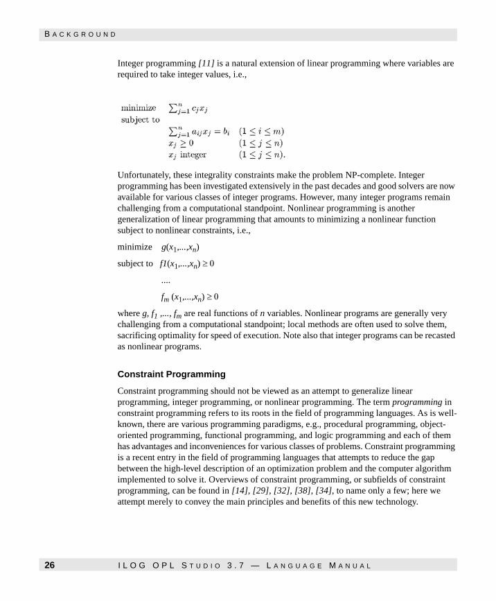
Integer programming [11] is a natural extension of linear programming where variables are required to take integer values, i.e.,
Unfortunately, these integrality constraints make the problem NP-complete. Integer programming has been investigated extensively in the past decades and good solvers are now available for various classes of integer programs. However, many integer programs remain challenging from a computational standpoint. Nonlinear programming is another generalization of linear programming that amounts to minimizing a nonlinear function subject to nonlinear constraints, i.e.,
minimize g(x1,...,xn)
subject to f1(x1,...,xn) ≥ 0
....
fm (x1,...,xn) ≥ 0
where g, f1 ,..., fm are real functions of n variables. Nonlinear programs are generally very challenging from a computational standpoint; local methods are often used to solve them, sacrificing optimality for speed of execution. Note also that integer programs can be recasted as nonlinear programs.
Constraint Programming
Constraint programming should not be viewed as an attempt to generalize linear programming, integer programming, or nonlinear programming. The term programming in constraint programming refers to its roots in the field of programming languages. As is well-known, there are various programming paradigms, e.g., procedural programming, object-oriented programming, functional programming, and logic programming and each of them has advantages and inconveniences for various classes of problems. Constraint programming is a recent entry in the field of programming languages that attempts to reduce the gap between the high-level description of an optimization problem and the computer algorithm implemented to solve it. Overviews of constraint programming, or subfields of constraint programming, can be found in [14], [29], [32], [38], [34], to name only a few; here we attempt merely to convey the main principles and benefits of this new technology.
26 I L O G O P L S T U D I O 3 . 7 — L A N G U A G E M A N U A L

B A C K G R O U N D
Intro
du
ction
What is Constraint Programming
The essence of constraint programming is a two-level architecture integrating a constraint and a programming component. The constraint component provides the basic operations of the architecture and consists of a system reasoning about fundamental properties of constraint systems such as satisfiability and entailment. The constraint component is often called the constraint store, by analogy to the memory store of traditional programming languages. The constraint store contains the constraints accumulated at some computation step and supports various queries and operations over these constraints. Operating around the constraint store is a programming-language component that specifies how to combine the basic operations, often in non-deterministic ways, since search is so fundamental in combinatorial optimization. The constraint and programming components can take many different forms depending upon the constraint system selected (e.g., linear constraints over reals) and the host programming languages (e.g., Prolog, C++). The constraint systems featured in early constraint programming languages such as Prolog II [5], Prolog III [4], CHIP [8], [31], CLP(ℜ) [15], and BNR-Prolog [19] included constraint systems based on linear programming, consistency techniques, interval reasoning, and Boolean unification. Recent constraint languages, or new versions of the pioneering languages, now include many new algorithms tailored to certain application areas. Typical examples include the edge-finder algorithm and its generalization for the scheduling applications and flow algorithms that are fundamental in a variety of resource-allocation applications. Since constraint programming originated from constraint logic programming, early programming components were based on the nondeterministic, goal-directed, computational model of Prolog. Concurrent constraint programming [16], [29], which is the foundation of constraint languages such as Oz [30] and cc(FD) [39], introduced a model in which the programming component is a set of agents communicating by adding constraints to, and querying, the constraint store. Concurrent constraint programming introduced constraint entailment as a basic operation and a constraint-driven computational model. Both of these features are now standard constraint programming technologies. Another important step in the development of modern constraint programming was the embedding of constraints in more traditional languages such as C and C++, as demonstrated, for instance, by ILOG Solver [22], [23] and 2LP [17]. Here the programming component is a traditional programming language extended to support nondeterminism and to support constraint systems as a basic data type.
Benefits of Constraint Programming
Constraint programming is an appealing technology in a variety of combinatorial search problems, since it can reduce the development time of these applications by orders of magnitude. The gain in productivity comes mainly from the high-level abstractions provided by constraint programming to support two fundamental activities of combinatorial optimization algorithms: constraint reasoning and search. For constraint reasoning, constraint programming languages embed sophisticated constraint-solving algorithms that are accessed simply by specifying a set of constraints to satisfy. For search, constraint programming languages provide nondeterministic constructs that relieve programmers of many mundane implementation aspects of tree-search procedures.
I L O G O P L S T U D I O 3 . 7 — L A N G U A G E M A N U A L 27

B A C K G R O U N D
As a consequence, solving a combinatorial optimization problem using a constraint programming language generally has two steps: generating the set of constraints to be satisfied (the constraint part) and describing how to search for solutions (the search part). The gain in productivity in constraint programming also comes from its declarative nature; a feature of course fundamental to modeling languages as well. Constraints specify properties of the solutions and can be thought of intuitively as restrictions on a space of possibilities. However, they do not specify a computational procedure for finding these solutions: i.e., constraints describe what the solutions are without specifying how to find them. This declarative nature of constraints has many benefits: the order in which constraints are imposed has no importance and additional constraints, that capture new properties of the solutions, can be added without worrying about the interaction with existing constraints and the search procedure. As a consequence, users can focus on the modeling aspects of the problem rather than on low-level programming details. Finally, the separation of the constraint and search parts also has some obvious software engineering benefits. It is possible to modify these components independently, e.g., one can change the search strategy without having to be concerned about the constraint-solving part.
Limitations of Constraint Programming
For many applications, however, the distance between the model and the constraint program is still large, mainly due to peculiarities of the host programming languages and lack of support for modeling. Constraint programming emerged from research on programming languages and there is a reluctance to sacrifice the general-purpose nature of these languages and a tendency to adopt a minimalist approach to extensions. However, the obvious trend at this point is to remedy this situation and to propose higher-level modeling tools.
Misconceptions about Constraint Programming
Before concluding this section, it is important to dispel two common misconceptions about constraint programming. The first misconception is that constraint programming is an extension of mathematical programming. In fact, mathematical programming and constraint programming really address orthogonal issues that arise in solving combinatorial optimization problems. Mathematical programming focuses on identifying classes of problems, studying their properties, and proposing algorithms for solving them. In contrast, constraint programming is concerned with proposing software architectures (i.e., ways of organizing computer programs) to simplify the implementation of combinatorial optimization algorithms. The goal here is to shorten the development time of combinatorial optimization algorithms by reducing the distance between a high-level design and an actual implementation. A second common misconception is that constraint programming does not use bounding techniques in optimization problems. In fact, constraint programming uses a variety of bounding techniques (e.g., linear programming relaxations or preemptive scheduling) and can combine several bounding techniques naturally. This misconception probably originates from the implicit nature of bounding procedures in constraint programming where bounding procedures are implemented as constraints that update the domains (e.g., the set of possible values) of the variables.
28 I L O G O P L S T U D I O 3 . 7 — L A N G U A G E M A N U A L

O P L
Intro
du
ction
For instance, to define a new bounding procedure in constraint programming, a new constraint of the form c(x1,..., xn, f) can be defined where x1,...,xn are the problem variables and f is the objective function. For a minimization problem, this constraint may add simpler constraints of the form f ≥ l at each node of the search tree (and, possibly, other constraints on the variables x1,...,xn ).
OPL
OPL is an attempt to combine the strengths of mathematical programming modeling languages and constraint programming. It aims both at increasing the applicability of modeling languages by incorporating techniques from constraint programming and at improving the expressive power of traditional constraint programming tools by borrowing ideas from modeling languages.
OPL as a Modeling Language
OPL shares many features with modeling languages such as AMPL. It supports traditional algebraic notations: a constraint such as
is written in OPL as
sum(j in 1..n) d[i,j] = s;
Similarly, the set of constraints
is written in OPL as
forall(i in 1..n) sum(j in 1..n) d[i,j] = s;
These features and others ensure that OPL preserves the traditional strengths of modeling languages in linear and integer programming. However, OPL goes beyond the traditional algebraic support of modeling languages by introducing logical combinations of constraints,
dijj 1–
n
∑ s=
dij s 1 i n≤ ≤( )–
j 1–
n
∑
I L O G O P L S T U D I O 3 . 7 — L A N G U A G E M A N U A L 29

O P L
higher-order constraints, and enumerated types for variables, and by letting indices of arrays contain variables. (Some of these features, all standard in constraint programming, have in fact recently been proposed as possible extensions of AMPL).
For instance, the OPL statement:
enum Country {Belgium,Denmark,France,Germany,Netherlands,Luxembourg}; enum Colors {red,blue,yellow,gray}; var Colors color[Country]; solve {color[France] <> color[Belgium]; color[France] <> color[Luxembourg]; color[France] <> color[Germany]; color[Luxembourg] <> color[Germany]; color[Luxembourg] <> color[Belgium]; color[Belgium] <> color[Netherlands]; color[Belgium] <> color[Germany]; color[Germany] <> color[Netherlands]; color[Germany] <> color[Denmark] };
colors a map of several European countries so that no two adjacent countries have the same color. The statement specifies the countries and the colors, declares an array of variables (one per country) that may take four colors, and states the constraints. It is difficult to imagine a much more concise statement of this problem. Note, however, that the statement involves variables ranging over enumerated values and "not equal" constraints, two features usually not supported in mathematical programming modeling languages. OPL also supports arbitrary logical combinations such as:
rankMen[m,o] < rankMen[m,wife[m]] => rankWomen[o,husband[o]] < rankWomen[o,m];
which illustrates the implication of two constraints. The example also shows the indexing of an array with variables or expressions involving variables, a very expressive modeling tool. In the above example, wife[m] and husband[o] are variables. Higher-order constraints are also a fundamental tool for modeling many applications.
For instance, the expression:
sum(j in Series) (s[j] = i)
counts the number of variables s[j] equal to i. Finally, OPL offers a rich set of modeling concepts for scheduling applications by including concepts such as activities and resources, also present in some constraint programming languages. By providing these novel modeling tools, OPL adds a new dimension to both modeling and constraint programming languages. It should enlarge the applicability of modeling languages and make constraint programming techniques more accessible.
30 I L O G O P L S T U D I O 3 . 7 — L A N G U A G E M A N U A L

O P L S C R I P T
Intro
du
ction
OPL as a Constraint Programming Language
Perhaps the most fundamental departure from mathematical programming modeling languages in OPL is its support for the programming component of the constraint programming architecture. OPL lets users specify search procedures using a variety of nondeterministic and constraint-driven constructs inspired by the development of constraint programming. As mentioned, this ability to specify how to explore the search space is fundamental to obtaining a reasonable efficiency in many problems and OPL provides high-level abstractions to support concise and effective specifications. Of course, OPL clearly separates the constraint and programming components, preserving and amplifying the spirit of constraint programming. A typical programming component in OPL is an instruction specifying what variables must be given values and in what order.
For instance, the instruction:
forall(s in Stores ordered by decreasing regretdmin(cost[s])) tryall(w in Warehouses ordered by increasing transportation[s,w]) supplier[s] = w;
specifies a maximal regret heuristics in a warehouse location problem that is studied in detail in Chapter 14, Constraint Programming. OPL also supports constraint-driven constructs inspired by concurrent constraint programming. By supporting both the constraint and the programming components of the constraint programming architecture, OPL adds a new dimension to modeling languages. No modeling language we are aware of supports the programming component.
OPLScript
As mentioned earlier, modeling languages are sometimes extended by a command language that makes it possible to interact with models, to solve several instances of the same model, and or to solve sequences of models. OPLScript is a script language for OPL supporting these functionalities.
The main novelty in OPLScript is to consider models as first-class objects, providing a clear separation of concerns between models and scripting and making the overall system
Note: The programming component discussed here is fundamentally different from the command language of AMPL and from OPLScript. The command language in AMPL and OPLScript are used, for instance, to allow users to solve a sequence of related problems and to design algorithms that solve related models (by calling external solvers to solve single instances of a model). The goal of the programming component in OPL is to specify the search strategy for a model, i.e., how to explore the search space of possible solutions. These two extensions are orthogonal and complementary.
I L O G O P L S T U D I O 3 . 7 — L A N G U A G E M A N U A L 31

C O N T E N T S
compositional. As a consequence, models can be developed, tested, and maintained independently from the scripts using them. In addition, since OPL supports the constraint programming architecture, it is possible to sequence models using different technologies, which is useful in many applications. For instance, it is possible to have one constraint programming model whose solutions are input configurations for a linear programming model that is responsible for choosing a subset of these configurations optimizing an objective function.
Contents
This book is a comprehensive presentation of OPL and OPLScript and is organized in three parts.
◆ Part I describes the modeling language itself; each chapter in this part reviews some aspect of OPL in detail. These technical chapters are preceded by a short tour of OPL to introduce the main concepts and the computation model.
◆ Part II applies OPL in three application areas: linear and integer programming, constraint programming, and scheduling.
◆ Part III describes OPLScript and its applications.
Model Conventions and Disclaimers
OPL and OPLScript statements and excerpts are printed in tt font and displayed in floating and numbered statements or enclosed between horizontal brackets, as in:
var int nbRabbits in 0..20; var int nbPheasants in 0..20; solve { 20 = nbRabbits + nbPheasants; 56 = 4*nbRabbits + 2*nbPheasants; };
The examples used in this book are intended to illustrate the functionalities of OPL and OPLScript. They should not be viewed as recommended or ultimate solutions for these problems. Indeed, better solutions can often be designed in some of the applications by exploiting more properties. These better solutions are, however, outside the scope of this book. Note also that the results displayed in this book are given only for the convenience of the readers and are not guaranteed to match exactly those of a specific implementation of OPL Studio.
32 I L O G O P L S T U D I O 3 . 7 — L A N G U A G E M A N U A L

C H A P T E R
A S
ho
rt Tou
r of O
PL
2
A Short Tour of OPL
This chapter, a brief tour of OPL, does not aim to cover all the features of OPL but rather to give readers a preliminary understanding of the language and its novel aspects. The chapter starts by presenting how OPL supports linear programming and its extensions, an area that is well covered in traditional modeling languages. The chapter then turns to the support provided by OPL for constraint programming and scheduling, two areas new in modeling languages.
Linear and Integer Programming
An optimization problem is typically specified by an objective function and a set of constraints over some variables. A solution to the problem is an assignment of values to the variables that satisfies the constraints and optimizes the value of the objective function. The purpose of an OPL statement is thus to express these two components for the application at hand. Consider a Belgian company Volsay, which specializes in producing ammoniac gas (N H3) and ammonium chloride (N H4 Cl). Volsay has at its disposal 50 units of nitrogen (N), 180 units of hydrogen (H), and 40 units of chlorine (Cl). The company makes a profit of 40 Belgian francs for each sale of an ammoniac gas unit and 50 Belgian francs for each sale of an ammonium chloride unit. Volsay would like a production plan maximizing its profits given its available stocks.
I L O G O P L S T U D I O 3 . 7 — L A N G U A G E M A N U A L 33

L I N E A R A N D I N T E G E R P R O G R A M M I N G
The OPL statement
var float+ gas; var float+ chloride; maximize 40 * gas + 50 * chloride subject to { gas + chloride <= 50; 3 * gas + 4 * chloride <= 180; chloride <= 40; };
formalizes this problem. It declares two real variables gas and chloride, representing the production of ammoniac gas and ammonium chloride. These variables are of type float+, which means that they are required to be nonnegative. The objective function
maximize 40 * gas + 50 * chloride
states that the profit must be maximized. The constraints ensure that the production plan does not exceed the available stocks of nitrogen, hydrogen, and chlorine, respectively. The constraint gas + chloride <= 50 represents the capacity constraint for nitrogen, since each unit of ammoniac gas and of ammonium chloride uses one unit of nitrogen. The next two constraints, for hydrogen and chlorine respectively, are similar in nature. As mentioned previously, a solution to an optimization problem is typically an assignment of values to the variables that satisfies the constraints and optimizes the objective function. OPL returns the optimal solution
Optimal Solution with Objective Value 2300.0000 gas = 20.0000 chloride = 30.0000
for the Volsay production-planning problem. This OPL statement is a linear programming model. As mentioned, linear programming is the class of problems that can be expressed as the optimization of a linear objective function subject to a set of linear constraints (i.e., linear equations and inequalities) over real numbers. Linear programming models can be solved for large numbers of variables and constraints and are, from a computational standpoint, the simplest applications considered in this book.
Arrays
The above statement is very specific to the application at hand. In general, it is desirable to write generic models that can be extended, modified easily, and applied in different contexts. The next two sections describe a number of OPL concepts to simplify the process of creating such models. A first step towards more genericity is the use of arrays, which makes it easier, for instance, to accommodate new products in the future.
The Volsay production-planning model can be rewritten using arrays as:
enum Products {gas, chloride}; var float+ production[Products]; maximize
34 I L O G O P L S T U D I O 3 . 7 — L A N G U A G E M A N U A L

A S
ho
rt Tou
r of O
PL
L I N E A R A N D I N T E G E R P R O G R A M M I N G
40 * production[gas] + 50 * production[chloride] subject to { production[gas] + production[chloride] <= 50; 3 * production[gas] + 4 * production[chloride] <= 180; production[chloride] <= 40; };
This new statement illustrates several features of the language. First, the instruction
enum Products {gas, chloride};
declares an enumerated set Products that represents the set of products of the company. The declaration
var float+ production[Products];
declares an array of two variables, production[gas] and production[chloride], to represent the optimal production of ammoniac gas and ammonium chloride. These variables are used in the rest of the statement, which remains essentially the same as before. As will become clear subsequently, one of the novel features of OPL is the generality of its arrays: OPL arrays can have an arbitrary number of dimensions and their index sets can be arbitrary finite sets, possibly involving complex data structures.
Data Declarations
A second fundamental step towards more genericity in the model amounts to representing the problem data explicitly. In addition to the products, the problem data obviously consists of the components (i.e., nitrogen, hydrogen, and chlorine), the demand of each product for each component, the profit of each product, and the stock available for each component. The following excerpt from an OPL statement
enum Products {gas, chloride}; enum Components {nitrogen, hydrogen, chlorine};
float+ demand[Products,Components] = [[1, 3, 0], [1, 4, 1]]; float+ profit[Products] = [40, 50]; float+ stock[Components] = [50, 180, 40];
declares and initializes these data. Components is an enumerated set that defines the chemical components necessary for the products, demand is a two-dimensional array whose element demand[p,c] represents the demand of product p for component c, and profit and stock are two arrays representing the profit of each product and the stock available for each component. The rest of the statement can be obtained easily by replacing the numbers by the relevant data items. For instance, the objective function is simply written as
maximize profit[gas]* production[gas] + profit[chloride] * production[chloride]
I L O G O P L S T U D I O 3 . 7 — L A N G U A G E M A N U A L 35

L I N E A R A N D I N T E G E R P R O G R A M M I N G
Aggregate Operators and Quantifiers
It should be clear, however, that the statement above contains much redundancy. All constraints, and all arithmetic terms in these constraints and in the objective function, are similar: they differ only in their indices.
Statement 2.1
Statement 2.1 A Simple Production Model (gas1.mod).
OPL has two features to factorize these commonalities, aggregate operators and quantifiers, which are used in the new model in Statement 2.1. The objective function
maximize sum(p in Products) profit[p] * production[p]
illustrates the use of the aggregate operator sum to take the summation of the individual profits. A variety of aggregate operators are available in OPL, including sum, prod, min, and max. The instruction
forall(c in Components) sum(p in Products) demand[p,c] * production[p] <= stock[c]
shows how the universal quantifier forall can be used to state closely related constraints. It generates one constraint for each chemical component, each constraint stating that the total demand for the component cannot exceed its available stock. OPL supports rich parameter specifications in aggregate operators and quantifiers, as will become clear in Chapter 4, Data Modeling.
enum Products {gas, chloride}; enum Components {nitrogen, hydrogen, chlorine};
float+ demand[Products,Components] = [[1, 3, 0], [1, 4, 1]]; float+ profit[Products] = [40, 50]; float+ stock[Components] = [50, 180, 40];
var float+ production[Products]; maximize sum(p in Products) profit[p] * production[p] subject to { forall(c in Components) sum(p in Products) demand[p,c] * production[p] <= stock[c] };
36 I L O G O P L S T U D I O 3 . 7 — L A N G U A G E M A N U A L

A S
ho
rt Tou
r of O
PL
L I N E A R A N D I N T E G E R P R O G R A M M I N G
Isolating the Data
Another fundamental step in making models reusable is to separate the model and the instance data. OPL Studio supports this clean separation through the notions of projects.
Statement 2.2
Statement 2.2 The Production Model (gas.mod).
A project is the association of a model (a file whose suffix is .mod) and a set of data files (files whose suffixes are .dat). The model declares the data but does not initialize them. The data files contain the initializations of each declared data item. Here we do not describe the details of OPL Studio, but generally describe applications by giving the model and the instance data separately. For instance, Statements 2.2 and 2.3 together describe a project for the Volsay production-planning problem. The model part is essentially the same as before, except that it declares the data but does not initialize it. A declaration of the form
float+ profit[Products] = ...;
declares the array profit and specifies that its initialization is given in a data file. The data file simply associates an initialization with each non-initialized piece of data.
enum Products ...; enum Components ...;
float+ demand[Products,Components] = ...; float+ profit[Products] = ...; float+ stock[Components] = ...;
var float+ production[Products]; maximize sum(p in Products) profit[p] * production[p] subject to { forall(c in Components) sum(p in Products) demand[p,c] * production[p] <= stock[p] }
I L O G O P L S T U D I O 3 . 7 — L A N G U A G E M A N U A L 37

L I N E A R A N D I N T E G E R P R O G R A M M I N G
Data Initialization
OPL offers a variety of ways to initialize data. One particularly useful feature is the possibility of associating indices with values to avoid various kinds of errors. Statement 2.4 illustrates this feature on the instance data for the Volsay production model.
Statement 2.3
Statement 2.3 Instance Data for the Production Model (gas.dat).
Statement 2.4
Statement 2.4 Instance Data for the Production Model (gasn.dat).
The initialization
profit = #[gas:30 chloride:40]#;
describes the initialization of array profit by associating the value 30 with index gas and the value 40 with index chloride. (Of course, the order of the pairs has no importance in these initializations.) When using index:value pairs, the delimiters #[ and ]# must be used instead of [ and ]. Note also that, in data files, the items can be initialized in any order and the commas can be omitted freely.
Records
OPL offers a variety of data structures in addition to arrays and enumerated sets. Records, a fundamental tool for structuring the application data, offer an alternative to the traditional approach of representing data in parallel arrays. To see the use of records in OPL, consider the following production-planning model. To meet the demands of its customers, a company
Products = {gas, chloride}; Components = {nitrogen, hydrogen, chlorine}; demand = [[1, 3, 0], [1, 4, 1]]; profit = [40, 50]; stock = [50, 180, 40];
Products = {gas chloride}; Components = {nitrogen hydrogen chlorine};
profit = #[gas:30 chloride:40]#; stock = #[nitrogen:50 hydrogen:180 chlorine:40]#; demand = #[ gas: #[nitrogen:1 hydrogen:3 chlorine:0]# chloride: #[nitrogen:1 hydrogen:4 chlorine:1]# ]#;
38 I L O G O P L S T U D I O 3 . 7 — L A N G U A G E M A N U A L
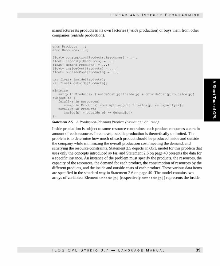
A S
ho
rt Tou
r of O
PL
L I N E A R A N D I N T E G E R P R O G R A M M I N G
manufactures its products in its own factories (inside production) or buys them from other companies (outside production).
Statement 2.5
Statement 2.5 A Production-Planning Problem (production.mod).
Inside production is subject to some resource constraints: each product consumes a certain amount of each resource. In contrast, outside production is theoretically unlimited. The problem is to determine how much of each product should be produced inside and outside the company while minimizing the overall production cost, meeting the demand, and satisfying the resource constraints. Statement 2.5 depicts an OPL model for this problem that uses only the concepts introduced so far, and Statement 2.6 on page 40 presents the data for a specific instance. An instance of the problem must specify the products, the resources, the capacity of the resources, the demand for each product, the consumption of resources by the different products, and the inside and outside costs of each product. These various data items are specified in the standard way in Statement 2.6 on page 40. The model contains two arrays of variables: Element inside[p] (respectively outside[p]) represents the inside
enum Products ...; enum Resources ...;
float+ consumption[Products,Resources] = ...; float+ capacity[Resources] = ...; float+ demand[Products] = ...; float+ insideCost[Products] = ...; float+ outsideCost[Products] = ...;
var float+ inside[Products]; var float+ outside[Products];
minimize sum(p in Products) (insideCost[p]*inside[p] + outsideCost[p]*outside[p]) subject to { forall(r in Resources) sum(p in Products) consumption[p,r] * inside[p] <= capacity[r]; forall(p in Products) inside[p] + outside[p] >= demand[p]; };
I L O G O P L S T U D I O 3 . 7 — L A N G U A G E M A N U A L 39

L I N E A R A N D I N T E G E R P R O G R A M M I N G
(respectively outside) production of product p. The objective function specifies that the production cost must be minimized.
Statement 2.6
Statement 2.6 Data for the Production-Planning Problem (production.dat).
The production cost is simply the sum of the individual production costs, which are obtained by multiplying the inside and outside productions of the given product by their respective costs. Finally, the model has two types of constraints. The first set of constraints expresses the capacity constraints, the second set states the demand constraints. The model is once again a linear programming problem and its output is as follows:
Optimal Solution with Objective Value 372.0000 inside[kluski] = 40.0000 inside[capellini] = 0.0000 inside[fettucine] = 0.0000 outside[kluski] = 60.0000 outside[capellini] = 200.0000 outside[fettucine] = 300.0000
Although the model is simple, it is inconvenient in separating the data associated with each product in different arrays: for instance, array demand stores the demand for the products, while array insideCost stores their inside costs. This technique, sometimes called parallel arrays, may be error-prone and less readable for more complicated models. Records provide a simple way to cluster related data and impose more structure on a model. This is illustrated in Statements 2.7 and 2.8, which exhibit an alternative model for the production-planning problem.
Products = {kluski capellini fettucine}; Resources = {flour eggs}; consumption = [ [0.5 0.2] [0.4 0.4] [0.3 0.6] ]; capacity = [20, 40]; demand = [100, 200, 300]; insideCost = [0.6, 0.8, 0.3]; outsideCost = [0.8, 0.9, 0.4];
40 I L O G O P L S T U D I O 3 . 7 — L A N G U A G E M A N U A L

A S
ho
rt Tou
r of O
PL
L I N E A R A N D I N T E G E R P R O G R A M M I N G
Statement 2.7
Statement 2.7 The Production-Planning Problem Revisited (product.mod).
Statement 2.8
Statement 2.8 Data for the Revised Production-Planning Problem (product.dat).
The instruction
struct ProductData { float+ demand; float+ insideCost; float+ outsideCost; float+ consumption[Resources]; };
declares a record type having four fields. The first three fields, of type float, are used to represent the demand and costs of a product; the last field is an array representing the resource consumptions of the product. These fields are intended to hold all the data related to a given product.
enum Products ...; enum Resources ...;
struct ProductData { float+ demand; float+ insideCost; float+ outsideCost; float+ consumption[Resources]; };
ProductData product[Products] = ...; float+ capacity[Resources] = ...;
var float+ inside[Products]; var float+ outside[Products];
minimize sum(p in Products) (product[p].insideCost*inside[p] + product[p].outsideCost*outside[p]) subject to { forall(r in Resources) sum(p in Products) product[p].consumption[r] * inside[p] <= capacity[r]; forall(p in Products) inside[p] + outside[p] >= product[p].demand; };
Products = {kluski capellini fettucine}; Resources = {flour eggs}; product = #[ kluski : <100, 0.6, 0.8, [0.5, 0.2]> capellini : <200, 0.8, 0.9, [0.4, 0.4]> fettucine : <300, 0.3, 0.4, [0.3, 0.6]> ]#; capacity = [20, 40];
I L O G O P L S T U D I O 3 . 7 — L A N G U A G E M A N U A L 41

L I N E A R A N D I N T E G E R P R O G R A M M I N G
The instruction
ProductData product[Products] = ...;
declares an array of these records, one for each product. The initialization
product = #[ kluski : <100 0.6 0.8 [0.5 0.2]> capellini : <200 0.8 0.9 [0.4 0.4]> fettucine : <300 0.3 0.4 [0.3 0.6]> ]#;
from Statement 2.8 on page 41 specifies these various data items: records are initialized by giving values for each of their fields. It is of course possible to use a named initialization for the record, as shown in Statement 2.9 on page 43, in which case the initialization is enclosed with #< and >#. Record fields can be obtained by postfixing the record with a dot and the field name. For instance, in the objective function
minimize sum(p in Products) (product[p].insideCost * inside[p] + product[p].outsideCost * outside[p])
The expression product[p].insideCost represents the field insideCost of the record product[p].
Similarly, in the constraint
forall(r in Resources) sum(p in Products) product[p].consumption[r] * inside[p] <= capacity[r];
The expression product[p].consumption represents the field consumption of record product[p]. This field is an array that can be subscripted in the traditional way.
Displaying Results
The statements presented so far did not specify elements of the solution which should be displayed. OPL, and OPL Studio in particular, offer a variety of ways to display and visualize the results of an application; Chapter 9, Display gives more detail on the display instructions. An interesting feature of OPL is the ability to display tuples of expressions. For instance, it is possible to enhance Statement 2.9 on page 43 with an instruction
display(p in Products) <inside[p],outside[p]>;
to produce the output
Optimal Solution with Objective Value 372.0 <inside[kluski],outside[kluski]> = <40.0,60.0> <inside[capellini],outside[capellini]> = <0.0,200.0> <inside[fettucine],outside[fettucine]> = <0.0,300.0>
42 I L O G O P L S T U D I O 3 . 7 — L A N G U A G E M A N U A L

A S
ho
rt Tou
r of O
PL
L I N E A R A N D I N T E G E R P R O G R A M M I N G
This display makes it possible to visualize the inside and outside productions of a product simultaneously.
Statement 2.9
Statement 2.9 Named Data for the Revised Production-Planning Problem (productn.dat)
OPL also makes it possible to visualize useful information about the model solution. For instance, the instruction
display(p in Products) <inside[p],inside[p].rc)>;
displays both the inside production of a product and its reduced cost:
Optimal Solution with Objective Value 372.0 <inside[kluski],reducedCost(inside[kluski])> = <40.0,0.0> <inside[capellini],reducedCost(inside[capellini])> = <0.0,0.06> <inside[fettucine],reducedCost(inside[fettucine])> = <0.0,0.02>
Integer Programming
The statements presented so far are all linear programming models. As mentioned previously, linear programs with very large numbers of variables and constraints can be solved efficiently. Unfortunately, this is no longer true when the variables are required to take integer values. Integer programming, the class of problems that can be expressed as the optimization of a linear function subject to a set of linear constraints over integer variables, is in fact NP-hard [10]. More important, perhaps, is the fact that the integer programs that can be solved in reasonable time are much smaller in size than their linear programming counterparts. There are exceptions, of course, and this book describes several important classes of integer programs which can be solved efficiently, but users of OPL should be
Products = {kluski capellini fettucine}; Resources = {flour eggs}; product = #[ kluski: #< demand:100 insideCost:0.6 outsideCost:0.8 consumption:[0.5 0.2] ># capellini: #< demand:200 insideCost:0.8 outsideCost:0.9 consumption:[0.4 0.4] ># fettucine: #< demand:300 insideCost:0.3 outsideCost:0.4 consumption:[0.3 0.6] ># ]#; capacity = [20, 40];
I L O G O P L S T U D I O 3 . 7 — L A N G U A G E M A N U A L 43

L I N E A R A N D I N T E G E R P R O G R A M M I N G
warned that discrete problems are in general much harder to solve than linear programs. A typical example of integer programs is the knapsack problem, which can be intuitively understood as follows. We have a knapsack with a fixed capacity (an integer) and a number of items. Each item has an associated weight (an integer) and an associated value (another integer). The problem consists of filling the knapsack without exceeding its capacity, while maximizing the overall value of its contents. A multi-knapsack problem is similar to the knapsack problem, except that there are multiple features for the object (e.g., weight and volume) and multiple capacity constraints. Statement 2.10 on page 44 depicts a model for the multi-knapsack problem, while Statement 2.11 on page 45 describes an instance of the problem.
This model has several novel features. It represents items and resources not by enumerated sets but rather by integers. In other words, the items (respectively the resources) are represented by successive integers starting at 1. The instructions
int nbItems = ...; int nbResources = ...; range Items 1..nbItems; range Resources 1..nbResources;
declare the number of items and the number of resources, as well as two ranges, Items and Resources, to represent the set of items and the set of resources.
Statement 2.10
Statement 2.10 A Multi-Knapsack Model (knapsack.mod).
int nbItems = ...; int nbResources = ...; range Items 1..nbItems; range Resources 1..nbResources; int capacity[Resources] = ...; int value[Items] = ...; int use[Resources,Items] = ...; int maxValue = max(r in Resources) capacity[r];
var int take[Items] in 0..maxValue; maximize sum(i in Items) value[i] * take[i] subject to forall(r in Resources) sum(i in Items) use[r,i] * take[i] <= capacity[r];
44 I L O G O P L S T U D I O 3 . 7 — L A N G U A G E M A N U A L

A S
ho
rt Tou
r of O
PL
L I N E A R A N D I N T E G E R P R O G R A M M I N G
Statement 2.11
Statement 2.11 Data for The Multi-Knapsack Problem (knapsack.dat)
The next three instructions
int capacity[Resources] = ...; int value[Items] = ...; int use[Resources,Items] = ...;
are similar to the data declarations presented earlier in this chapter. The array capacity represents the capacity of the resources, the array value the value of each item, and use[r,i] the use of resource r by item i. The next instruction
int maxValue = max(r in Resources) capacity[r];
is more interesting. It declares an integer maxValue whose value is given by an expression. We see later in Chapter 4, Data Modeling that OPL has many features for computing and preprocessing data, since this is fundamental in simplifying and improving the efficiency of many models. The instruction
var int take[Items] in 0..maxValue;
declares the problem variables: take[i] represents the number of times item i is selected in the solution. The variable is of type integer and is restricted to range in 0..maxValue.
The rest of the statement is rather standard and should raise no difficulty. Here is the solution to the instance specified in Statement 2.11 on page 45:
Optimal Solution with Objective Value 261922 take[1] = 0 take[2] = 0 take[3] = 0 take[4] = 154 take[5] = 0 take[6] = 0 take[7] = 0 take[8] = 913 take[9] = 333 take[10] = 0 take[11] = 6499 take[12] = 1180
nbResources = 7; nbItems = 12; capacity= [18209 7692 1333 924 26638 61188 13360]; value= [96 76 56 11 86 10 66 86 83 12 9 81]; use = [ [19 1 10 1 1 14 152 11 1 1 1 1] [0 4 53 0 0 80 0 4 5 0 0 0] [4 660 3 0 30 0 3 0 4 90 0 0] [7 0 18 6 770 330 7 0 0 6 0 0] [0 20 0 4 52 3 0 0 0 5 4 0] [0 0 40 70 4 63 0 0 60 0 4 0] [0 32 0 0 0 5 0 3 0 660 0 9]];
I L O G O P L S T U D I O 3 . 7 — L A N G U A G E M A N U A L 45

L I N E A R A N D I N T E G E R P R O G R A M M I N G
Although integer programs are, in general, substantially harder to solve than linear programs, they have also been the topic of intensive investigation. OPL recognizes when a statement is an integer programming model and applies an efficient integer programming algorithm.
Mixed Integer-Linear Programming
OPL can also solve models that include both integer and real variables, generally known as mixed integer-linear programs (MILP). OPL approaches them in essentially the same way as integer programs except, of course, that branching takes place only on integer variables. Consider the following application involving mixing some metals into an alloy. The metal may come from several sources: in pure form or from raw materials, scraps from previous mixes, or ingots. The alloy must contain a certain amount of the various metals, as expressed by a production constraint specifying lower and upper bounds for the quantity of each metal in the alloy. Each source also has a cost and the problem consists of blending the sources into the alloy while minimizing the cost and satisfying the production constraints. Similar problems arise in other domains, e.g., the oil, paint, and the food processing industries. Statements 2.12 and 2.13 depict a model for the problem, while Statement 2.14 on page 47 depicts some instance data.
Model Data
The model is described in terms of a number of constants specifying the various types of metals, raw materials, scrap, and ingots. In the instance, there are three metals, two raw materials, two kinds of scrap, and one kind of ingot. The model also defines ranges for each of the components. It then defines the cost of the various components in costMetal, costRaw, costScrap, costIngo. In the instance data, for example, the second raw material has a cost of 5. The data items low and up specify the production constraints and give lower and upper bounds on the quantity of each sort of metal in the alloy. For example, in the instance data, between 30% and 40% of the alloy must be the second metal. The next data items, percRaw, percScrap, and percIngo, specify the percentage of each metal in the sources. In our instance, for example, the second type of scrap contains 1% of the first metal, none of the second metal, and 70% of the third metal. Finally, the data alloy specifies the amount of alloy to be produced.
Model Variables
The model variables specify how much of each source is used in the alloy: the array p specifies the quantities of pure metals, array r specifies the quantities of raw materials, array s specifies the quantities of scrap, array i specifies the number of ingots. All variables are of type float except number of ingots, which are integers. The problem is thus a mixed integer-linear program. The instruction
var float m[j in Metals] in low[j] * alloy .. up[j] * alloy;
is particularly interesting, since it shows how to specify the range of variables in a generic fashion. More precisely, the range of variables m[j] is given by the expression low[j] * alloy .. up[j] * alloy. Note also that the model uses the variables in array m as intermediary variables to represent the quantity of each metal produced.
46 I L O G O P L S T U D I O 3 . 7 — L A N G U A G E M A N U A L

A S
ho
rt Tou
r of O
PL
L I N E A R A N D I N T E G E R P R O G R A M M I N G
Statement 2.12
Statement 2.12 A Blending Problem: Part I (blending.mod)
Statement 2.13
Statement 2.13 A Blending Problem: Part II (blending.mod).
Statement 2.14
Statement 2.14 Instance Data for the Blending Problem (blending.dat).
int nbMetals = ...; int nbRaw = ...; int nbScrap = ...; int nbIngo = ...;
range Metals 1..nbMetals; range Raws 1..nbRaw; range Scraps 1..nbScrap; range Ingos 1..nbIngo;
float+ costMetal[Metals] = ...; float+ costRaw[Raws] = ...; float+ costScrap[Scraps] = ...; float+ costIngo[Ingos] = ...; float+ low[Metals] = ...; float+ up[Metals] = ...; float+ percRaw[Metals,Raws] = ...; float+ percScrap[Metals,Scraps] = ...; float+ percIngo[Metals,Ingos] = ...;
int+ alloy = ...;
var float+ p[Metals]; var float+ r[Raws]; var float+ s[Scraps]; var int+ i[Ingos] in 0..maxint; var float m[j in Metals] in low[j] * alloy .. up[j] * alloy; minimize sum(j in Metals) costMetal[j] * p[j] + sum(j in Raws) costRaw[j] * r[j] + sum(j in Scraps) costScrap[j] * s[j] + sum(j in Ingos) costIngo[j] * i[j] subject to { forall(j in Metals) m[j] = p[j] + sum(k in Raws) percRaw[j,k] * r[k] + sum(k in Scraps) percScrap[j,k] * s[k] + sum(k in Ingos) percIngo[j,k] * i[k] sum(j in Metals) m[j] = alloy; };
nbMetals = 3; nbRaw = 2; nbScrap = 2; nbIngo = 1; costMetal = [22 10 13]; costRaw = [6 5]; costScrap = [7 8]; costIngo = [9]; low = [0.05 0.30 0.60]; up = [0.10 0.40 0.80]; percRaw = [[0.20 0.01] [0.05 0.00] [0.05 0.30]]; percScrap = [[0.00 0.01] [0.60 0.00] [0.40 0.70]]; percIngo = [[0.10] [0.45] [0.45]]; alloy = 71;
I L O G O P L S T U D I O 3 . 7 — L A N G U A G E M A N U A L 47

L I N E A R A N D I N T E G E R P R O G R A M M I N G
Model Constraints
There are two types of constraints in this problem. The first
forall(j in Metals) m[j] = p[j] + sum(k in Raws) percRaw[j,k] * r[k] + sum(k in Scraps) percScrap[j,k] * s[k] + sum(k in Ingos) percIngo[j,k] * i[k]
makes sure that the right amounts of metal are produced. The amount m[j] of metal j must be equal to the amount of pure metal p[j] added to the quantity of metal j contained in the raw materials, the scrap, and the ingots. The correct amount of metals are computed using the percentage of metals contained in the sources. The last constraint
sum(j in Metals) m[j] = alloy;
makes sure that the various metals produced give the correct amount of alloy. The objective function in this model is rather simple. It consists of computing the price of each source from its unit price (e.g., costMetal) and the amount produced (e.g., p[j]). When given the model and the instance data, OPL returns the solution
Optimal Solution with Objective Value 653.6100 p[1] = 0.0467 p[2] = 0.0000 p[3] = 0.0000
r[1] = 0.0000 r[2] = 0.0000
s[1] = 17.4167 s[2] = 30.3333
i[1] = 32
m[1] = 3.5500 m[2] = 24.8500 m[3] = 42.6000
48 I L O G O P L S T U D I O 3 . 7 — L A N G U A G E M A N U A L

A S
ho
rt Tou
r of O
PL
C O N S T R A I N T P R O G R A M M I N G
Constraint Programming
The most novel aspect of OPL compared to other mathematical modeling languages lies in its support for constraint programming. Constraint programming, a recent entry in the programming languages arena, is in essence a two-level architecture consisting of:
◆ a constraint component: a constraint-solving system reasoning about fundamental properties of constraints such as satisfiability and entailment;
◆ a programming component: a programming language specifying how to generate, combine, and process constraints, often in nondeterministic ways.
Constraint programming support in OPL is discussed in detail in Chapter 14, Constraint Programming. Here we give a brief introduction to its constraint programming features. Consider finding an eight digit number that is a square and remains a square when 1 is concatenated in front of its decimal notation. Here is a simple OPL solution to the problem:
var int n in 10000000..99999999; var int x in 0..20000; var int y in 0..20000; solve { n = x*x; 100000000+n = y*y; };
The statement declares three variables: the variable n, which is the desired result, and two variables x and y, which are used to state the constraints. The range of variable n is chosen to represent the fact that n is a eight-digit number, while the ranges of x and y were chosen in order not to eliminate any solution. The solve instruction specifies the problem constraints in terms of the variables. Note that the two constraints are nonlinear and that there is no objective function. When OPL encounters a statement that is not a linear, an integer, or a mixed integer linear program, its basic strategy is to use the problem constraints to reduce the domains (i.e., the set of possible values) of the variables. The constraints specify which combinations of these values are solutions of the problem and OPL uses various relaxations of these constraints to prune the search space, i.e., the domains of the variables. Sometimes constraint solving alone is sufficient to find a solution to the problem of interest. However, in general, the constraint-solving process does not locate a solution either because there are multiple solutions or because the constraint-solving algorithms are not strong enough, since they were designed as a trade-off between computational complexity and pruning. For the above problem, constraint solving alone produces the following domain reductions:
n in [23765625..56250000] x in [4875..7500] y in [11125..12500]
by using reasoning on the range of the variables.
I L O G O P L S T U D I O 3 . 7 — L A N G U A G E M A N U A L 49

C O N S T R A I N T P R O G R A M M I N G
To find a solution to this problem, OPL must generate values for the variables. In particular, OPL assigns a value, say 23765625, to n and applies its constraint-solving algorithm with this new assumption. If constraint solving fails (i.e., if there is no solutions to this problem), OPL backtracks. Backtracking undoes all the changes to the domains of the variables to restore the same computational state as before the nondeterministic choice. OPL then continues its execution by trying another value for n. The process terminates when OPL finds a solution or determines that there are no solutions (if all possible assignments lead to failure). On the above example, OPL returns the solution
Solution [1] n = 23765625 x = 4875 y = 11125
It is also possible to ask OPL to produce all solutions or obtain other solutions incrementally. When asked to find all solutions, OPL returns the two solutions:
Solution [1] n = 23765625 x = 4875 y = 11125
Solution [2] n = 56250000 x = 7500 y = 12500
As can be seen, OPL has default strategies to search for solutions. However, for more advanced applications, it is often desirable to provide strategies tailored to the problem at hand. In the above example, the default strategy consists of generating a value for all variables, which is equivalent to the statement
var int n in 10000000..99999999; var int x in 0..20000; var int y in 0..20000; solve { n = x*x; 100000000+n = y*y };
search { generate(n); generate(x); generate(y); };
50 I L O G O P L S T U D I O 3 . 7 — L A N G U A G E M A N U A L

A S
ho
rt Tou
r of O
PL
C O N S T R A I N T P R O G R A M M I N G
Statement 2.15
Statement 2.15 The Eight-Queens Problem (queens8.mod).
The above statement includes a search procedure that tells OPL to generate values for n, x, and y. This is a fundamental novelty in modeling languages: OPL makes it possible to state concisely not only the problem constraints but also how to search for solutions. An interesting example illustrating this novel functionality is described later in this chapter. To understand constraint programming in more detail, it is useful to consider the n-queens problem, which consists of placing n queens on a chessboard of size n x n so that no two queens attack each other. Since no two queens can be placed on the same column, a simple model of this problem consists of associating a queen with each column and searching for an assignment of rows to the queens that no two queens are placed on the same row and the same diagonal. Statement 2.15 on page 51 depicts an OPL statement for the eight-queens problems. The statement has a number of interesting features. It first declares an array of eight variables, all of which take their value in the range 1...8. The solve instruction defines the problem constraints, i.e., that no two queens should attack each other. The basic idea here is to generate for all 1 ≤ i < j ≤ 8 the constraints
queens[i] <> queens[j] queens[i] + i <> queens[j] + j queens[i] - i <> queens[j] - j
Statement 2.16
Statement 2.16 The n-Queens Model (queens.mod).
where the symbol <> means "not-equal". OPL uses a single universal quantifier for parameters i and j and specifies that these parameters are ordered, i.e., i < j. Such a construct is useful in many applications to make statements shorter and more explicit. Note also that the statement is not an integer programming model, since integer programming only supports linear equations and inequalities (and not strict inequalities such as <, >, and <>). Statement 2.16 on page 51 generalizes the problem to an arbitrary number of queens. It
var int queens[1..8] in 1..8; solve { forall(ordered i, j in 1..8) { queens[i] <> queens[j]; queens[i] + i <> queens[j] + j; queens[i] - i <> queens[j] - j; }};
int n << "number of queens:"; range Domain 1..n;
var Domain queens[Domain]; solve { forall(ordered i,j in Domain) { queens[i] <> queens[j]; queens[i] + i <> queens[j] + j; queens[i] - i <> queens[j] - j }};
I L O G O P L S T U D I O 3 . 7 — L A N G U A G E M A N U A L 51

C O N S T R A I N T P R O G R A M M I N G
declares an integer that, when executed, prints the message Number of queens: and requests an integer from the user. It is interesting at this point to study how OPL behaves on this problem. To illustrate the computational model, consider first the five-queens problem. Constraint solving does not reduce the domains of the variables initially. OPL thus generates a value, say 1, for one of its variables, say queens[1]. After this nondeterministic assignment, constraint solving removes inconsistent values from the domains of queens[2],...,queens[5], as depicted in Figure 2.1. The next step of the generation process tries the value 3 for queens[2]. OPL then removes inconsistent values from the domains of the remaining queens (see Figure 2.2 on page 53). Since only one value remains for queens[3] and queens[4], these values are immediately assigned by OPL to these variables and, after more constraint solving, OPL assigns the value 4 to queens[5]. A solution to the five-queens problem is thus found with two choices and without backtracking.
It is also interesting to consider the eight-queens problem after three choices. Figure 2.3 on page 53 depicts an intermediate stage when some (but not all) constraint solving has taken place. Since only one value is left for queens[6], OPL assigns this value and propagates the constraints further. This assigns the value 7 to queens[8] which, in turn, assigns the value 2 to queens[7] and the value 8 to queens[4] (see Figure 2.4 on page 54). As a consequence, queens[5] has no value left in its domain and constraint solving fails. OPL then backtracks and tries another value for queens[3].
Figure 2.1
Figure 2.1 The Five-Queens Problem After One Choice.
52 I L O G O P L S T U D I O 3 . 7 — L A N G U A G E M A N U A L

A S
ho
rt Tou
r of O
PL
C O N S T R A I N T P R O G R A M M I N G
Figure 2.2
Figure 2.2 The Five-Queens Problem After Two Choices.
Figure 2.3
Figure 2.3 The Eight-Queens Problem After Three Choices (Intermediate I).
I L O G O P L S T U D I O 3 . 7 — L A N G U A G E M A N U A L 53

C O N S T R A I N T P R O G R A M M I N G
Figure 2.4
Figure 2.4 The Eight-Queens Problem After Three Choices (Intermediate II).
It is useful to mention at this point that OPL does not necessarily generate values for the queens in the order queens[1] to queens[n]. In fact, the default strategy of OPL (which is implemented in instruction generate) chooses first the variable with the fewest possible values. This heuristic, known as the first-fail principle, is in general effective in reducing the size of the search space by discovering failures early. To generate values for the queens in the order queens[1] to queens[n], it is sufficient to write the following search procedure:
search { forall(i in Domain) generate(queens[i]); };
Statement 2.17
Statement 2.17 The Magic-Series Model (magic1.mod).
int n << "Number of Variables:";
range Range 0..n-1; range Domain 0..n;
var Domain s[Range]; solve { forall(i in Range) s[i] = sum(j in Range) (s[j] = i); };
54 I L O G O P L S T U D I O 3 . 7 — L A N G U A G E M A N U A L

A S
ho
rt Tou
r of O
PL
C O N S T R A I N T P R O G R A M M I N G
Higher-Order Constraints
The magic-series problem has become a traditional constraint-programming benchmark and illustrates convincingly the use of higher-order constraints. The problem consists of finding a magic series, i.e., a sequence of numbers S = (s0,s1,....,sn) such that si represents the number of occurrences of i in S. For instance, (1, 2, 1, 0) is a magic series for n = 3, since there is one occurrence of 0, two occurrences of 1, one occurrence of 1 and zero occurrences of 3. Statement 2.17 on page 54 depicts an OPL model for this problem. The most interesting aspect of this statement is the constraint specification, which expresses the occurrence constraints using higher-order constraints. An expression
sum(j in Range) (s[j] = i)
is used to count the number of variables in s[0],...,s[n-1] equal to i. The novelty here is that the summation is over relations of the form s[j] = i and not over traditional expressions. The key insight to understanding this summation is to realize that the OPL implementation replaces each constraint appearing in an expression by a 0-1 variable (i.e., an integer variable ranging over 0...1) that is assigned the value 1 if the constraint is satisfied and 0 if it is violated. It is thus easy to see that the above statement exactly captures the problem constraints. In addition, constraints can be combined in OPL using the traditional logical connectives. It is also interesting to see how OPL uses higher-order constraints during constraint solving. The key idea is to propagate information in both directions: from the constraint to its associated 0-1 variable and from the 0-1 variable to its associated constraint. In the first direction, OPL tries to determine whether the constraint is satisfied.
Statement 2.18
Statement 2.18 The Magic-Series Problem With Redundant Constraints (magic2.mod).
The satisfiability of the constraint is determined locally on the basis of the domains of the variables. For instance, if x is a variable ranging over 5...10 and y a variable ranging over 1...3, OPL determines that x > y is satisfied, in which case its associated 0-1 variable is assigned the value 1. For the same domain, OPL would also determine that the constraint x < y is violated, in which case its associated 0-1 variable is assigned the value 0. However, if y ranges over 1...6, OPL cannot determine whether x > y is satisfied or violated, since there exist assignments that satisfy the constraint and assignments that violate it. In the second direction, OPL uses the 0-1 variable to insert new constraints. For instance, if the 0-1
int n << "Number of Variables:";
range Range 0..n-1; range Domain 0..n;
var Domain s[Range]; solve { forall(i in Range) s[i] = sum(j in Range) (s[j] = i); sum(i in Range) s[i] = n; sum(i in Range) s[i]*i = n; };
I L O G O P L S T U D I O 3 . 7 — L A N G U A G E M A N U A L 55

C O N S T R A I N T P R O G R A M M I N G
variable associated with x > y is assigned to 1 (by using the constraint in which the higher-order constraint appears), OPL inserts the constraint x > y. On the other hand, if the 0-1 variable associated with x > y is assigned to 0, OPL inserts the constraint x ≤ y. Statement 2.18 on page 55 depicts another OPL model for the magic-series problem, that contains two additional "redundant" (or surrogate) constraints. The constraints are redundant since they do not remove any solution compared to the previous statement. They are, however, interesting from a computational standpoint, since they express some fundamental properties of the problem that the OPL implementation cannot deduce automatically. However, the OPL implementation can exploit them to reduce the search space and obtain solutions faster. The first of these redundant constraints expresses that the sum of the elements in the series is n, which is obviously true since there are n variables. The second constraint expresses the same information but computes the sum differently by using products of the form s[i] * i (i.e., the value i times its number of occurrences).
Finally, we show a formulation of the magic-series problem using the global constraint distribute.
Statement 2.19
Statement 2.19 The Magi-Series Problem With the Global Constraint distribute (magic3.mod).
Global constraints, a fundamental tool for solving a variety of combinatorial optimization problems in OPL, enforce complex relationships among a number of variables. They are discussed in more detail in Chapter 5, Expressions and Constraints. Given a one-dimensional array occurrence of index set S, a one-dimensional array value with the same index set S, and a one-dimensional array element,
distribute(occurrence,value,element)
holds if occurrence[i] is the number of occurrences of value[i] in array element. The effect of distribute could be implemented by a conjunction of higher-order constraints but achieves the same pruning more efficiently. Statement 2.19 on page 56 shows the magic-series problem with this global constraint. Besides the use of the higher-order constraint, Statement 2.19 also introduces a novel concept: the generic initialization of an array. The declaration
int value[i in Range] = i;
int n << "Number of Variables:";
range Range 0..n-1; range Domain 0..n;
int value[i in Range] = i;
var Domain s[Range]; solve { distribute(s,value,s); sum(i in Range) s[i] = n; sum(i in Range) s[i]*i = n; };
56 I L O G O P L S T U D I O 3 . 7 — L A N G U A G E M A N U A L

A S
ho
rt Tou
r of O
PL
C O N S T R A I N T P R O G R A M M I N G
declares an array of n integers: value[0] to value[n-1]. These integers are assigned generically to the values 0 to n - 1 by using a parameter i ranging over Range. As will become clear, generic initializations are also a fundamental tool in OPL for facilitating the model specification.
Statement 2.20
Statement 2.20 A Map-Coloring Problem (map.mod)
Variables over Enumerated Sets
In the models presented so far, variables ranged over integer or real values. In OPL, it is also possible to declare variables taking values in an enumerated set. This feature is interesting in avoiding the mapping from enumerated values into integers. Consider a map-coloring application entailing coloring a map of various European countries so that no two adjacent countries have the same color. Statement 2.20 on page 57 gives an OPL model to solve this problem. The statement uses two enumerated sets to denote the countries and the colors (more colors are unnecessary since every map can be colored with at most four colors). The statement also declares an array of variables, each variable in the array ranging over the colors. The constraints specify that adjacent countries be assigned different colors. Here is the first solution returned by OPL:
Solution [1] color[Belgium] = blue; color[Denmark] = red; color[France] = red; color[Germany] = yellow; color[Netherlands] = red; color[Luxembourg] = gray;
enum Country {Belgium,Denmark,France,Germany,Netherlands,Luxembourg}; enum Colors {blue,red,yellow,gray};var Colors color[Country]; solve { color[France] <> color[Belgium]; color[France] <> color[Luxembourg]; color[France] <> color[Germany]; color[Luxembourg] <> color[Germany]; color[Luxembourg] <> color[Belgium]; color[Belgium] <> color[Netherlands]; color[Belgium] <> color[Germany]; color[Germany] <> color[Netherlands]; color[Germany] <> color[Denmark]; };
I L O G O P L S T U D I O 3 . 7 — L A N G U A G E M A N U A L 57

C O N S T R A I N T P R O G R A M M I N G
Variables and Expressions as Indices
We now illustrate another feature of constraint programming: the use of variables, and of expressions involving variables, to index arrays. This feature is fundamental in obtaining concise and clear models for many combinatorial optimization problems. This section illustrates the gain in expressiveness on the stable marriage problem, and also shows that constraints can be combined with Boolean connectives. The similarity between the OPL statement and the natural language specification is striking.
The problem can be described as follows. Consider a group of women and a group of men who must marry and assume that each person has indicated a ranking for her/his possible spouses. The problem is to find a matching between the two groups such that the marriages are stable. The definition of stability is interesting: a marriage between m and w is stable provided that
◆ whenever m prefers another person o to w, o prefers her/his spouse to m.
◆ whenever w prefers another person o to m, o prefers her/his spouse to w.
Intuitively, m and w may be unhappy but they are bound to stay together. An instance of this problem is depicted in Table 2.1 and Table 2.2, where a lower ranking indicates a stronger preference. For instance, the first row in Table 2.1 says that Richard is Helen's first choice (rank 1) and, Greg is her last choice (rank 5). Statement 2.21 on page 59 depicts an OPL model for the stable marriage problem and Statement 2.22 on page 60 presents the data for this instance. The model data consists of two enumerated types for specifying the women and men and of rankings given by the women and by the men. The model is expressed in terms of two arrays of variables: wife, which specifies the men's wives, and husband, which specifies the women's husbands. Variables in array wife must take their values in enumerated set Women, while variables in array husband must take their values in set Men. The constraints in this problem are of course the interesting and novel part. The first two sets of constraints guarantee that a solution is a set of marriages by ruling out the possibility that a man be married to a woman who is married to another man (and vice-versa).
Table 2.1 Ranking of the Women in the Stable Marriage Problem.
Richard James John Hugh Greg
Helen 1 2 4 3 5
Tracy 3 5 1 2 4
Linda 5 4 2 1 3
Sally 1 3 5 4 2
Wanda 4 2 3 5 1
58 I L O G O P L S T U D I O 3 . 7 — L A N G U A G E M A N U A L

A S
ho
rt Tou
r of O
PL
C O N S T R A I N T P R O G R A M M I N G
Statement 2.21
Statement 2.21 The Stable Marriage Problem (marriage.mod).
Table 2.2 Ranking of the Men in the Stable Marriage Problem.
Helen Tracy Linda Sally Wanda
Richard 5 1 2 4 3
James 4 1 3 2 5
John 5 3 2 4 1
Hugh 1 5 4 3 2
Greg 4 3 2 1 5
enum Women ...; enum Men ...;
int rankWomen[Women,Men] = ... int rankMen[Men,Women] = ...
var Women wife[Men]; var Men husband[Women]; solve { forall(m in Men) husband[wife[m]] = m;
forall(w in Women) wife[husband[w]] = w;
forall(m in Men & o in Women) rankMen[m,o] < rankMen[m,wife[m]] => rankWomen[o,husband[o]] < rankWomen[o,m];
forall(w in Women & o in Men) rankWomen[w,o] < rankWomen[w,husband[w]] => rankMen[o,wife[o]] < rankMen[o,w];}
I L O G O P L S T U D I O 3 . 7 — L A N G U A G E M A N U A L 59

C O N S T R A I N T P R O G R A M M I N G
Statement 2.22
Statement 2.22 Instance Data for the Stable Marriage Problem (marriage.dat).
The model satisfies this requirement by stating the spouse of the spouse of a person is the person herself, i.e.,
forall(m in Men) husband[wife[m]] = m; forall(w in Women) wife[husband[w]] = w;
It is important to recognize here that husband and wife are arrays of variables, so that an expression such as husband[wife[m]] indexes an array of variables with a variable. This feature is critical in this example to state the constraints in a simple way. The constraint-solving algorithm of OPL knows how to use these expressions to reduce the domains of the variables in the arrays husband and wife using bidirectional propagation.
The remaining constraints specify the stability requirement and are almost direct translations of the definition. The set of constraints
forall(m in Men & o in Women) rankMen[m,o] < rankMen[m,wife[m]] => rankWomen[o,husband[o]] < rankWomen[o,m];
states that, if a man m prefers a woman o to his wife (i.e., the rank of o is less than the rank of his wife), then o prefers her husband to m. The last set of constraints
forall(w in Women & o in Men) rankWomen[w,o] < rankWomen[w,husband[w]] => rankMen[o,wife[o]] < rankMen[o,w];
handles the symmetric case. The OPL model uses a logical implication together with the possibility of having variables index an array to make this statement simple and natural.
Men = {Richard,James,John,Hugh,Greg}; Women = {Helen,Tracy,Linda,Sally,Wanda}; rankWomen = #[ Helen : #[Richard:1, James:2, John:4, Hugh:3, Greg:5]#, Tracy : #[Richard:3, James:5, John:1, Hugh:2, Greg:4]#, Linda : #[Richard:5, James:4, John:2, Hugh:1, Greg:3]#, Sally : #[Richard:1, James:3, John:5, Hugh:4, Greg:2]#, Wanda : #[Richard:4, James:2, John:3, Hugh:5 Greg:1]# ]#;
rankMen = #[ Richard : #[Helen:5, Tracy:1 , Linda:2 , Sally:4 , Wanda:3]#, James : #[Helen:4, Tracy:1 , Linda:3 , Sally:2 , Wanda:5]#, John : #[Helen:5, Tracy:3 , Linda:2 , Sally:4 , Wanda:1]#, Hugh : #[Helen:1, Tracy:5 , Linda:4 , Sally:3 , Wanda:2]#, Greg : #[Helen:4, Tracy:3 , Linda:2 , Sally:1 , Wanda:5]# ]#;
60 I L O G O P L S T U D I O 3 . 7 — L A N G U A G E M A N U A L
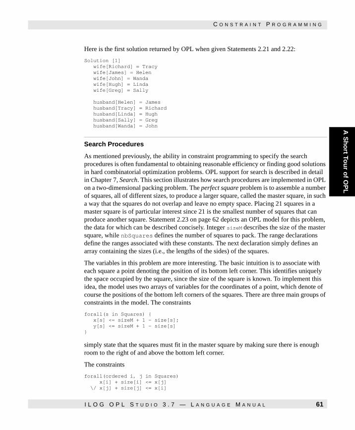
A S
ho
rt Tou
r of O
PL
C O N S T R A I N T P R O G R A M M I N G
Here is the first solution returned by OPL when given Statements 2.21 and 2.22:
Solution [1] wife[Richard] = Tracy wife[James] = Helen wife[John] = Wanda wife[Hugh] = Linda wife[Greg] = Sally
husband[Helen] = James husband[Tracy] = Richard husband[Linda] = Hugh husband[Sally] = Greg husband[Wanda] = John
Search Procedures
As mentioned previously, the ability in constraint programming to specify the search procedures is often fundamental to obtaining reasonable efficiency or finding good solutions in hard combinatorial optimization problems. OPL support for search is described in detail in Chapter 7, Search. This section illustrates how search procedures are implemented in OPL on a two-dimensional packing problem. The perfect square problem is to assemble a number of squares, all of different sizes, to produce a larger square, called the master square, in such a way that the squares do not overlap and leave no empty space. Placing 21 squares in a master square is of particular interest since 21 is the smallest number of squares that can produce another square. Statement 2.23 on page 62 depicts an OPL model for this problem, the data for which can be described concisely. Integer sizeM describes the size of the master square, while nbSquares defines the number of squares to pack. The range declarations define the ranges associated with these constants. The next declaration simply defines an array containing the sizes (i.e., the lengths of the sides) of the squares.
The variables in this problem are more interesting. The basic intuition is to associate with each square a point denoting the position of its bottom left corner. This identifies uniquely the space occupied by the square, since the size of the square is known. To implement this idea, the model uses two arrays of variables for the coordinates of a point, which denote of course the positions of the bottom left corners of the squares. There are three main groups of constraints in the model. The constraints
forall(s in Squares) { x[s] <= sizeM + 1 - size[s]; y[s] <= sizeM + 1 - size[s] }
simply state that the squares must fit in the master square by making sure there is enough room to the right of and above the bottom left corner.
The constraints
forall(ordered i, j in Squares) x[i] + size[i] <= x[j] \/ x[j] + size[j] <= x[i]
I L O G O P L S T U D I O 3 . 7 — L A N G U A G E M A N U A L 61

C O N S T R A I N T P R O G R A M M I N G
\/ y[i] + size[i] <= y[j] \/ y[j] + size[j] <= y[i];
express the fact that the squares may not overlap by using a disjunction of constraints. Two squares i and j do not overlap if square i is on the left
x[i] + size[i] <= x[j]
Statement 2.23
Statement 2.23 The Perfect Square Problem (square.mod).
on the right
x[j] + size[j] <= x[i]
below
y[i] + size[i] <= y[j]
or above square j
y[j] + size[j] <= y[i]
The last set of constraints
forall(p in Positions) {
int sizeM = 112; int NbSquares = 21; range Squares 1..NbSquares, range Positions 1..sizeM; int size[Squares] = [50,42,37,35,33,29,27,25,24,19,18,17,16,15,11,9,8,7,6,4,2]; var Positions x[Squares], var Positions y[Squares];
solve { forall(s in Squares) { x[s] <= sizeM + 1 - size[s]; y[s] <= sizeM + 1 - size[s] }; forall(ordered i, j in Squares) x[i] + size[i] <= x[j] \/ x[j] + size[j] <= x[i] \/ y[i] + size[i] <= y[j] \/ y[j] + size[j] <= y[i]; forall(p in Positions) { sum(s in Squares) size[s] * (x[s] <= p & p <= x[s] + size[s] - 1) = sizeM; sum(s in Squares) size[s] * (y[s] <= p & p <= y[s] + size[s] - 1) = sizeM; } }; search { forall(p in Positions) forall(s in Squares) try x[s] = p | x[s] <> p endtry; forall(p in Positions) forall(s in Squares) try y[s] = p | y[s] <> p endtry; };
62 I L O G O P L S T U D I O 3 . 7 — L A N G U A G E M A N U A L

A S
ho
rt Tou
r of O
PL
C O N S T R A I N T P R O G R A M M I N G
sum(s in Squares) size[s] * (x[s] <= p & p <= x[s] + size[s] - 1) = sizeM; sum(s in Squares) size[s] * (y[s] <= p & p <= y[s] + size[s] - 1) = sizeM }
are redundant constraints that exploit the knowledge that there is no empty space in the master square. The basic intuition here consists of drawing a vertical (respectively horizontal) line and retrieving the squares intersecting the line. Since there is no empty space, the sizes of the intersecting squares must be equal to the size of the master square. The intersection for the vertical line is computed simply by testing if the line is between the x-coordinates of the left and right corners, i.e.,
(x[s] <= p & p <= x[s] + size[s] - 1)
These expressions should be viewed as 0-1 variables. Multiplying them by the size of the squares makes it possible to sum the sizes of all intersecting squares and it is then sufficient to state that the sum must be equal to the size of the master square. The most novel aspect in this problem is, of course, the search procedure, which directly exploits the structure of the problem. The key idea is, once again, to use the fact that the master square has no empty space. As a consequence, the model considers each x- and y-position in the master square and chooses, in a nondeterministic way, whether each square starts at this position (it considers first the entire x-axis before moving to the y-axis). Most of the search is in fact spent in searching for the x-coordinates of the squares. The search procedure
search { forall(p in Positions) forall(s in Squares) try x[s] = p | x[s] <> p endtry; forall(p in Positions) forall(s in Squares) try y[s] = p | y[s] <> p endtry; };
captures this strategy. The instruction
forall(p in Positions) forall(s in Squares) try x[s] = p | x[s] <> p endtry;
considers all positions along the x-axis. For each such position p, the instruction considers all squares and nondeterministically chooses if the square starts (x[s]=p) or does not start (x[s] <> p) at position p. The instruction
forall(p in Positions) forall(s in Squares) try y[s] = p | y[s] <> p endtry;
applies the same principle to the y-axis. This choice strategy, together with the redundant constraints, helps OPL prune the search space substantially. Of course, the choice process considers both the x- and the y-coordinates.
I L O G O P L S T U D I O 3 . 7 — L A N G U A G E M A N U A L 63

S C H E D U L I N G
Scheduling
The other novel aspect of OPL is its support for scheduling applications, which are ubiquitous in industry. The OPL implementation uses specialized algorithms for scheduling applications that can reduce the search space substantially. Scheduling applications in OPL are discussed in Chapter 15, Scheduling; this section merely illustrates some of the concepts on a simple application. The application is scheduling the activities necessary to build a house. Table 2.3 depicts the activities, their duration, and the precedence constraints. For instance, facade is an activity of duration 2 that can start only when plumbing and roofing are completed. In addition, each activity costs an amount proportional to its duration. This amount, to be paid at the beginning of the activity, is $1,000 per day. The total budget is of course $29,000. Only $20,000 is available at the beginning of the project; the remaining $9,000 becomes available 15 days thereafter. The goal of the application is of course to minimize the project duration subject to the precedence and budget constraints. Statement 2.24 on page 66 depicts an OPL model for this application. The purpose here is not to explain in full detail all concepts in the model, but to give a feeling of the kind of support provided by OPL on scheduling applications. The main concept in scheduling application is the notion of activity, which is the association of two integer variables: a starting date and a duration.
Table 2.3 Activities and Precedences for the House Problem
Name Duration Precedences
masonry 7 {}
carpentry 3 {masonry}
roofing 1 {carpentry}
plumbing 8 {masonry}
facade 2 {plumbing, roofing}
windows 1 {roofing}
garden 1 {roofing, plumbing}
ceiling 3 {masonry}
painting 2 {ceiling}
moving 1 {windows, facade, garden, painting}
completion 0 {moving}
64 I L O G O P L S T U D I O 3 . 7 — L A N G U A G E M A N U A L

A S
ho
rt Tou
r of O
PL
S C H E D U L I N G
The instruction
Activity a[t in Tasks](duration[t]);
declares an array a of activities. The array is indexed by an enumerated set and activity a[t] has duration duration[t]. The starting dates of these activities are the primary output of the model. The instruction
DiscreteResource budget(29000);
declares the budget as a discrete resource with capacity 29,000. Activities are able to consume this budget, as becomes clear below. Resources are the second main scheduling concept, and OPL supports a variety of resources, including unary and discrete resources and reservoirs. Instructions of the form
a[masonry] precedes a[carpentry];
specify the precedence constraints of the application. The constraint specifies that the starting date of activity carpentry is greater or equal to the end date of activity masonry. The instruction
capacityMax(budget,0,15,20000);
specifies that the capacity of budget is only 20,000 for the first 15 days. The final constraint
forall(t in Tasks) a[t] consumes(1000*duration[t]) budget;
specifies that activity a[t] consumes the budget in a quantity proportional to its duration. Note that the objective function is to minimize the end date of the last activity. Here is the optimal solution returned by OPL for Statement 2.24 on page 66:
Optimal Solution with Objective Value: 21 a[masonry] = [0 -- 7 --> 7] a[carpentry] = [7 -- 3 --> 10] a[plumbing] = [7 -- 8 --> 15] a[ceiling] = [15 -- 3 --> 18] a[roofing] = [10 -- 1 --> 11] a[painting] = [18 -- 2 --> 20] a[windows] = [11 -- 1 --> 12] a[facade] = [15 -- 2 --> 17] a[garden] = [15 -- 1 --> 16] a[moving] = [20 -- 1 --> 21]
It specifies, for instance, that activity ceiling starts at time 15, has a duration of 3, and is completed by time 18. The same application can be solved using a set of strings instead of an enumerated type. Statement 2.25 on page 67 describes this functionality.
I L O G O P L S T U D I O 3 . 7 — L A N G U A G E M A N U A L 65

S C H E D U L I N G
Strings are used very much like enumerated types: they can appear in records and index arrays. See the section Strings on page 76 for a discussion of their respective advantages and inconveniences.
Statement 2.24
Statement 2.24 The House Problem (house2.mod).
enum Tasks { masonry, carpentry, plumbing, ceiling, roofing, painting, windows,facade,garden,moving};
int duration[Tasks] = [7,3,8,3,1,2,1,2,1,1];
Activity a[t in Tasks](duration[t]);
DiscreteResource budget(29000);
minimize a[moving].end subject to { a[masonry] precedes a[carpentry]; a[masonry] precedes a[plumbing]; a[masonry] precedes a[ceiling]; a[carpentry] precedes a[roofing]; a[ceiling] precedes a[painting]; a[roofing] precedes a[windows]; a[roofing] precedes a[facade]; a[plumbing] precedes a[facade]; a[roofing] precedes a[garden]; a[plumbing] precedes a[garden]; a[windows] precedes a[moving]; a[facade] precedes a[moving]; a[garden] precedes a[moving]; a[painting] precedes a[moving]; capacityMax(budget,0,15,20000); forall(t in Tasks) a[t] consumes(1000*duration[t]) budget; };
66 I L O G O P L S T U D I O 3 . 7 — L A N G U A G E M A N U A L

A S
ho
rt Tou
r of O
PL
N O T E S A N D R E F E R E N C E S
Notes and References
The Volsay problem is taken from course notes from the Jean Fichefet's 1984 operations research class at the University of Namur. The production and mixing problems are adapted from a similar problem in [26]. The first constraint-programming solution of the magic series was presented in [31]. The first models presented are based on the constraint program presented in [37]. The model with constraint distribute is based on [28]. The first constraint program for the stable marriage problem was presented in [28], the model presented here is significantly simpler. See [12] for a comprehensive discussion of the stable marriage problem. The perfect square problem and its variants have attracted much attention in the constraint-programming community. Colmerauer [4] presents a program to fill a rectangle with squares of different sizes using linear equations, inequalities, and disequations over rational numbers. The sizes of the rectangles are not known and the resulting program is a beautiful constraint program. Aggoun and Beldiceanu [1] present a CHIP program that solves the perfect square problem when the sizes of the squares are given. The program uses a specialized cumulative constraint and exploits the link between cumulative constraints and packing in two dimensions. The model described in this chapter was inspired by a program in [33] whose basic idea was suggested by Alain Colmerauer. The house problem is taken from [27].
Statement 2.25
Statement 2.25 The House Problem with Strings (strhouse2.mod).
{string} Tasks = { "masonry", "carpentry", "plumbing", "ceiling", "roofing", "painting", "windows", "facade", "garden", "moving" }; int duration[Tasks] = [7,3,8,3,1,2,1,2,1,1]; scheduleHorizon = 30; Activity a[t in Tasks](duration[t]); DiscreteResource budget(29000); minimize a["moving"].end subject to { a["masonry"] precedes a["carpentry"]; a["masonry"] precedes a["plumbing"]; a["masonry"] precedes a["ceiling"]; a["carpentry"] precedes a["roofing"]; a["ceiling"] precedes a["painting"]; a["roofing"] precedes a["windows"]; a["roofing"] precedes a["facade"]; a["plumbing"] precedes a["facade"]; a["roofing"] precedes a["garden"]; a["plumbing"] precedes a["garden"]; a["windows"] precedes a["moving"]; a["facade"] precedes a["moving"]; a["garden"] precedes a["moving"]; a["painting"] precedes a["moving"]; capacityMax(budget,0,15,20000); forall(t in Tasks) a[t] consumes(1000*duration[t]) budget; };
I L O G O P L S T U D I O 3 . 7 — L A N G U A G E M A N U A L 67

N O T E S A N D R E F E R E N C E S
68 I L O G O P L S T U D I O 3 . 7 — L A N G U A G E M A N U A L

C H A P T E R
Mo
dels
3
Models
This brief chapter fixes the syntactic conventions used in this book and describes the overall structure of OPL models.
Syntactic Conventions
The following conventions are used to describe the grammar of OPL: terminal symbols are denoted in typewriter font (e.g., solve), nt denotes a nonterminal symbol nt, [ object ] denotes an optional grammar segment object, { object } denotes zero, one, or several times the grammar segment object, object+ denotes an expression object { , object } while object* denotes an expression object { ; object } When a nonterminal symbol, say n, is defined by several rules, say a, b, and c, we use the notation
or
n → a | b | c
depending on convenience in context.
n → a
→ b
→ c
I L O G O P L S T U D I O 3 . 7 — L A N G U A G E M A N U A L 69

T E R M I N A L S Y M B O L S
Terminal Symbols
The basic building blocks of OPL are integers (terminal Integer), floating-point numbers (terminal Float), identifiers (terminal Id), strings (terminal string), and the keywords of the language (e.g., forall). Identifiers in OPL start with a letter and can contain only letters, digits, and the symbol – . Note that letters in OPL are case-sensitive. Integers are sequences of digits, possibly prefixed by a minus sign. Floats can be described in decimal notation (e.g., 3.4 or -2.5) or in scientific notation (e.g., 3.5e-3 or -3.4e10). The OPL reserved words are listed in Table 3.1 on page 71. Comments in OPL (and OPLScript()) are written in between /* and */ as in
/* This is a multi-line comment */
The characters // also start a comment that terminates at the end of the line on which they occur as in
var int cost in 0..maxCost; // objective function
Partial Grammar 3.1
Partial Grammar 3.1 The Syntax of Models.
Model → {Decl}
→ Instr
→ [ Search ]
→ [ OnSolution ]
→ { Display }
→ { Data }
70 I L O G O P L S T U D I O 3 . 7 — L A N G U A G E M A N U A L

Mo
dels
O P L K E Y W O R D S
OPL Keywords
Table 3.1 provides an alphabetical list of the reserved words in OPL.
Table 3.1 Reserved Words of OPL
Activity adjustLeft adjustRight adjustInternal
all alldifferent AlternativeResources applyStrategy
assert assignAlternatives basicPropagation BasisStatus
BFmaximize BFminimize BFSearch branch
branchDirGlobal branchDirLow branchDirUp branchLow
branchUp break breakable breakOnDuration
by capacityMax capacityMin case
circuit constraint consumes cout
data DBconnection DBexecute DBmapping
DBread DBupdate DDSearch decreasing
diff DiscreteEnergy DiscreteResource disjunctive
display distribute do edgeFinder
else endif endtry enum
evaluated excludesAllStates excludesState extendedPropagation
fail failLimit firstSolution float
forall from generate generateMax
generateMin generateSeq generateSize IDFSearch
if import in include
increasing infinity initialize int
inter SBSearch let linear
max maximize maxint maxof
min minimize minof mipsearch
mod not of ofile
I L O G O P L S T U D I O 3 . 7 — L A N G U A G E M A N U A L 71

M O D E L S
Models
The structure of OPL models is depicted in Partial Grammar 3.1 on page 70. An OPL statement consists of a sequence of declarations, an instruction, a search procedure, a sequence of display instructions, and a sequence of data initializations. The declarations, search procedure, displays, and data initializations are all optional. The following chapters describe each of these components in detail.
once onDomain onFailure onRange
onSolution onValue Open ordered
path periodicBreak piecewise postponed
precedes predicate prod produces
provides range rank rankFirst
rankGlobal rankLast rankLocal rankNotFirst
rankNotlast relaxation requires requiresAnyState
requiresState Reservoir return scheduleHorizon
scheduleOrigin search searchLimit searchStrategy
select selectFF selectMin selectMax
sequence set setAdjustField setBranchingDirection
setFloatField setof setPrecision setPriority
setTimes setting SheetConnection SheetRead
solve split splitLow splitUp
StateResource strategy string struct
subject subset sum symdiff
then timeLimit to transitionType
try tryall tryRankFirst tryRankLast
UnaryResource under union using
var visualize when while
with linear relaxation
Table 3.1 Reserved Words of OPL (Continued)
72 I L O G O P L S T U D I O 3 . 7 — L A N G U A G E M A N U A L

C H A P T E R
Data M
od
eling
4
Data Modeling
This chapter describes the basic concepts available for modeling data in OPL. You will find information on the following topics:
◆ Basic Data Types on page 56 reviews the basic types, i.e., integers, floats, and enumerated values.
◆ Data Structures on page 62 describes how these basic types can be combined using arrays, records, and sets to obtain complex data structures.
◆ Variables on page 72 shows how to declare variables in OPL.
◆ Data Types for Scheduling Applications on page 73 describes specific modeling tools for scheduling applications.
◆ Constraint Declarations on page 80 shows how to declare constraints.
◆ Data Consistency on page 80 discusses assertions to check data consistency.
◆ Initialization on page 81 describes data initialization.
◆ Partial Grammar 4.1 on page 56 describes the high-level syntax of data modeling declarations.
Note that predicate declarations are described in Chapter 5, Expressions and Constraints, while setting declarations are discussed in Chapter 10, Algorithmic Settings.
I L O G O P L S T U D I O 3 . 7 — L A N G U A G E M A N U A L 73

B A S I C D A T A T Y P E S
Partial Grammar 4.1
Partial Grammar 4.1 The Syntax of Declarations.
Basic Data Types
The three basic data types available in OPL are integers, floats, and enumerated values.
Integers
OPL provides the subset of the integers ranging from -231 to 231 as a basic data type. OPL also contains the integer constant maxint, which represents the largest positive integer available. A declaration of the form
int a = 25;
declares an integer a whose value is 25. It is also possible to declare natural numbers (i.e., nonnegative integers) using a declaration of the form
int+ a = 25;
When declaring natural numbers, OPL automatically checks whether the value used in the initialization is nonnegative. An execution error is raised when this is not the case. The initialization of an integer can be specified by an expression. For instance, the declaration
int n = 3; int size = n*n;
Decl → TypeDecl;
→ DataDecl;
→ VarDecl;
→ ActivityDecl;
→ ResourceDecl;
→ ConstraintDecl;
→ Assert;
→ Initialize;
→ ScheduleInit;
→ SettingDecl;
→ PredicateDecl;
→ DBDecl;
→ SheetDecl;
→ StrategyDecl;
74 I L O G O P L S T U D I O 3 . 7 — L A N G U A G E M A N U A L

Data M
od
eling
B A S I C D A T A T Y P E S
initializes size as the square of n. Expressions are covered in detail in Chapter 5, Expressions and Constraints. Integers can also be initialized by querying users. A declaration such as
int nbQueens << "Number of Queens:";
queries users with the message "number of queens:" and expects an integer, which is then used to initialize nbQueens.
Floats
OPL also provides a subset of the real numbers as the basic data type float. The implementation of floats in OPL obeys the IEEE 754 standard for floating-point arithmetic and the data type float in OPL uses double-precision floating-point numbers. OPL also has a predefined float constant infinity to represent the IEEE infinity symbol. Declarations of floats are essentially similar to declarations of integers. The declaration
float f = 3.2;
declares a float f whose value is 3.2. Once again, the value of the float can be specified by an arbitrary expression. Nonnegative floats play a special role in mathematical programming and are supported directly in OPL. For instance, the declaration
float+ f = 4.0;
declares a nonnegative float f. Once again, OPL checks if the initialization actually produces a nonnegative value and raises an error otherwise.
Enumerated Types
Enumerated types are an integral part of many programming languages and help produce more readable programs. Enumerated types in OPL are similar in spirit to those of the programming languages C and Pascal and are specified by listing their values. For instance, the declaration
enum Days {Monday, Tuesday, Wednesday, Thursday, Friday, Saturday, Sunday};
declares the enumerated type Days that consists of the values Monday, Tuesday, Wednesday, Thursday, Friday, Saturday, and Sunday. The names in an enumerated type have a global scope and cannot be used in any other enumerated type. Once an enumerated type T is declared, it is possible to declare data of type T. For instance, the declaration
Days myFavoriteDay = Sunday;
declares a data item myFavoriteDay of type Days and initializes it to Sunday. Of course, it is possible to define arrays and sets of type Days, as shown later in this chapter.
I L O G O P L S T U D I O 3 . 7 — L A N G U A G E M A N U A L 75
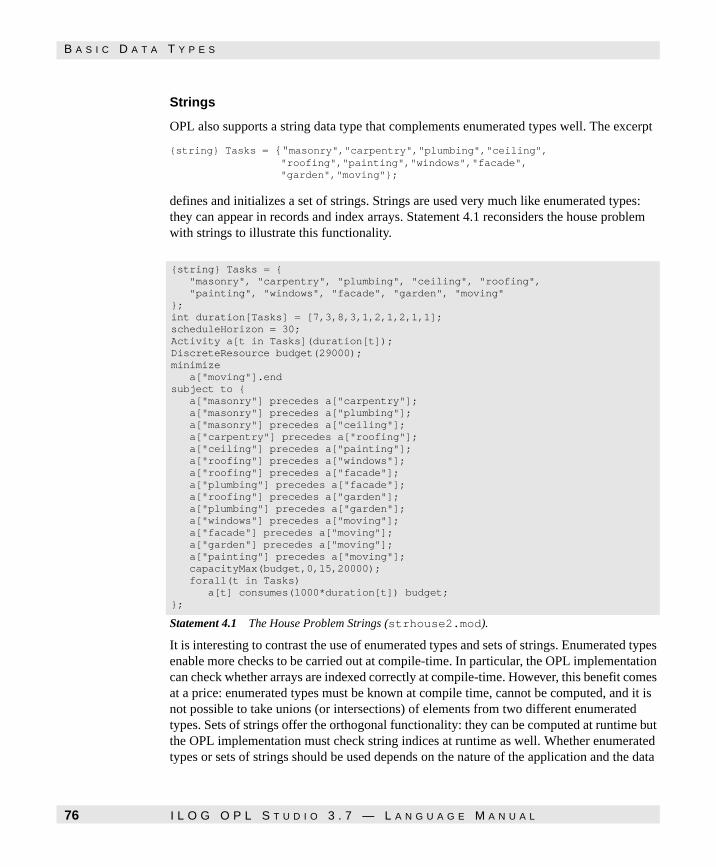
B A S I C D A T A T Y P E S
Strings
OPL also supports a string data type that complements enumerated types well. The excerpt
{string} Tasks = {"masonry","carpentry","plumbing","ceiling", "roofing","painting","windows","facade", "garden","moving"};
defines and initializes a set of strings. Strings are used very much like enumerated types: they can appear in records and index arrays. Statement 4.1 reconsiders the house problem with strings to illustrate this functionality.
Statement 4.1
Statement 4.1 The House Problem Strings (strhouse2.mod).
It is interesting to contrast the use of enumerated types and sets of strings. Enumerated types enable more checks to be carried out at compile-time. In particular, the OPL implementation can check whether arrays are indexed correctly at compile-time. However, this benefit comes at a price: enumerated types must be known at compile time, cannot be computed, and it is not possible to take unions (or intersections) of elements from two different enumerated types. Sets of strings offer the orthogonal functionality: they can be computed at runtime but the OPL implementation must check string indices at runtime as well. Whether enumerated types or sets of strings should be used depends on the nature of the application and the data
{string} Tasks = { "masonry", "carpentry", "plumbing", "ceiling", "roofing", "painting", "windows", "facade", "garden", "moving" }; int duration[Tasks] = [7,3,8,3,1,2,1,2,1,1]; scheduleHorizon = 30; Activity a[t in Tasks](duration[t]); DiscreteResource budget(29000); minimize a["moving"].end subject to { a["masonry"] precedes a["carpentry"]; a["masonry"] precedes a["plumbing"]; a["masonry"] precedes a["ceiling"]; a["carpentry"] precedes a["roofing"]; a["ceiling"] precedes a["painting"]; a["roofing"] precedes a["windows"]; a["roofing"] precedes a["facade"]; a["plumbing"] precedes a["facade"]; a["roofing"] precedes a["garden"]; a["plumbing"] precedes a["garden"]; a["windows"] precedes a["moving"]; a["facade"] precedes a["moving"]; a["garden"] precedes a["moving"]; a["painting"] precedes a["moving"]; capacityMax(budget,0,15,20000); forall(t in Tasks) a[t] consumes(1000*duration[t]) budget; };
76 I L O G O P L S T U D I O 3 . 7 — L A N G U A G E M A N U A L

Data M
od
eling
B A S I C D A T A T Y P E S
representation. Note that strings are required to use the database functionalities described in Chapter 11, Databases.
The string data type is endowed with a rich interface listed in Table 4.1 to manipulate a string and its content.
The semantics are defined as follows:
◆ int length()
Returns the string length in characters.
◆ char charAt(int i)
Returns the character at offset i. The method returns character ci in the string c0 c1 c2...cn-1 of length n when i belongs to 0..n - 1. It raises an error otherwise.
◆ string setAt(char ch,int ofs)
Returns a copy of the string where the character at offset ofs is replaced by ch.
◆ string concat(string s)
Table 4.1 The String Interface: Synopsis
Method Type
int length() char charAt(int ofs) string setAt(char ch,int ofs) string concat(string s) string prefix(int l) string suffix(int l) string subString(int o,int l) int indexOf(char ch) int lastIndexOf(char ch) int indexOf(int from,char ch) int lastIndexOf(int from,char ch) int matchAt(string s) string replaceChar(char ch,char by) string replaceCharOnce(char ch,char by) string replaceString(string s1,string s2) string replaceStringOnce(string s1,string s2) string toUpper() string toLower() int intValue() int toInt() float floatValue() float toFloat()
I L O G O P L S T U D I O 3 . 7 — L A N G U A G E M A N U A L 77

B A S I C D A T A T Y P E S
Returns the concatenation of the two input strings.
◆ string prefix(int l)
Returns the prefix of length l.
◆ string suffix(int l)
Returns the suffix of length l.
◆ string subString(int o,int l)
Returns a substring of the input starting at offset o and spanning l characters.
◆ int indexOf(char ch)
Returns the offset of the first occurrence of character ch.
◆ int lastIndexOf(char ch)
Returns the offset of the last occurrence of character ch.
◆ int indexOf(int from,char ch)
Returns the offset of the first occurrence of character ch in the suffix starting at offset from..
◆ int lastIndexOf(int from,char ch)
Returns the offset of the last occurrence of character ch in the prefix ending at offset from..
◆ int matchAt(string s)
Returns the offset of the first match of the input string with s within the input string.
◆ string replaceChar(char ch,char by)
Returns a copy of the input string where all occurrences of ch are replaced by the character by.
◆ string replaceCharOnce(char ch,char by)
Returns a copy of the input string where the first occurrence of ch is replaced by the character by.
◆ string replaceString(string s1,string s2)
Returns a copy of the input string where all the occurrences of the substring s1 are replaced by the substring s2.
◆ string replaceStringOnce(string s1,string s2)
Returns a copy of the input string where the first occurrence of the substring s1 is replaced by the substring s2.
◆ string toUpper()
78 I L O G O P L S T U D I O 3 . 7 — L A N G U A G E M A N U A L

Data M
od
eling
B A S I C D A T A T Y P E S
Returns a copy of the input string where all the Roman alphabet characters are replaced by their uppercase.
◆ string toLower()
Returns a copy of the input string where all the Roman alphabet characters are replaced by their lowercase.
◆ int intValue()
Returns an integer whose value is equal to the integer interpretation of the string in base 10. Conversion stops as soon as a non-digit character is encountered.
◆ int toInt()
Is a synonym for intValue().
◆ float floatValue()
Returns a floating point value equal to the floating point interpretation of the string in fixed point or scientific notation.
◆ float toFloat()
Is a synonym for floatValue().
I L O G O P L S T U D I O 3 . 7 — L A N G U A G E M A N U A L 79

D A T A S T R U C T U R E S
Characters
OPL supports a character oriented data type that inter-operates seamlessly with the integer and string types. The excerpt
char ch = ’a’;
declares and initializes the constant ch to the character ‘a’. The char type can be used anywhere in a model (i.e., in indexes, sets, records and arrays) except for the declaration of a variable domain. OPL provides several convenience methods on integers, strings and characters to convert a value from one representation to another. To represent characters, OPL relies upon the ASCII code. Integers can be converted to characters with the method char toChar() defined on the int type. Similarly, characters can be converted to integers (their ASCII code) with the method int intValue() defined on characters. Finally, the string type supports several methods to manipulate the content of a string at the character level. The methods supported by the string type are documented in the section Strings on page 58. The excerpt:
char c = ‘a’; int i = c.intValue(); char d = i.toChar();
illustrates a conversion of the character ‘a’ back and forth between the two representations.
Data Structures
More complex data types can be built from the basic data types. This section gives an overview of the basic data structures available in OPL, i.e., ranges, arrays, records, and sets.
Ranges
Integer ranges are fundamental in OPL, since they are often used in arrays and variable declarations, as well as in aggregate operators, queries, and quantifiers. An integer range is specified by giving its lower and upper bounds, as in
range Rows 1..10;
which declares a range 1..10. The lower and upper bounds can also be given by expressions, as in
int n = 8; range Rows [n+1..2*n+1];
Note that ranges are normally given in between brackets. If the lower bound is a number (i.e., an integer or a float), then the brackets can be omitted. Once a range has been defined, it is possible to declare data taking their values in this range. For instance, the declarations
range R 1..10; R r = 8; R v[1..3] = [1, 2, 3];
80 I L O G O P L S T U D I O 3 . 7 — L A N G U A G E M A N U A L

Data M
od
eling
D A T A S T R U C T U R E S
defines an integer r ranging in R and an array whose elements range in R. Once again, OPL checks whether the initialization produces a value inside the range and raises an error otherwise. OPL also supports the declaration of float ranges that specify a subset of the reals. For example:
range float fr 1.2..2.2;
specifies the subset of the reals in the interval [1.2,2.2].
Arrays
Arrays are, of course, fundamental in many applications; this section reviews the support for arrays available in OPL.
One-Dimensional Arrays
One-dimensional arrays are the simplest arrays in OPL and vary according to the type of their elements and index sets. A declaration of the form
int a[1..4] = [10, 20, 30, 40];
declares an array of four integers a[1],...,a[4] whose values are 10, 20, 30, and 40. It is of course possible to define arrays of other basic types. For instance, the instructions
int+ a[1..4] = [10, 20, 30, 40]; float f[1..4] = [1.2, 2.3, 3.4, 4.5]; Days d[1..2] = [Monday, Wednesday];
declare arrays of natural numbers, floats, and enumerated values, respectively. The index sets of arrays in OPL are very general and can be integer ranges, enumerated types, and arbitrary finite sets. In the examples so far, index sets were given explicitly, but it is possible to use a previously defined range, as in
range R 1..4; int a[R] = [10, 20, 30, 40];
The declaration:
int a[Days] = [10, 20, 30, 40, 50, 60, 70];
describes an array indexed by an enumerated type; its elements are a[Monday],...,a[Sunday]. Arrays can also be indexed by finite sets of arbitrary types. This feature is fundamental in OPL to exploit sparsity in large linear programming applications, as discussed in detail in Chapter 13, Linear and Integer Programming.
I L O G O P L S T U D I O 3 . 7 — L A N G U A G E M A N U A L 81
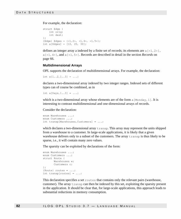
D A T A S T R U C T U R E S
For example, the declaration:
struct Edge { int orig; int dest; }; {Edge} Edges = {<1,2>, <1,4>, <1,5>}; int a[Edges] = [10, 20, 30];
defines an integer array a indexed by a finite set of records; its elements are a[<1,2>], a[<1,4>], and a[<1,5>]. Records are described in detail in the section Records on page 66.
Multidimensional Arrays
OPL supports the declaration of multidimensional arrays. For example, the declaration:
int a[1..2,1..3] = ...;
declares a two-dimensional array indexed by two integer ranges. Indexed sets of different types can of course be combined, as in
int a[Days,1..3] = ...;
which is a two-dimensional array whose elements are of the form a[Monday,1]. It is interesting to contrast multidimensional and one-dimensional arrays of records.
Consider the declaration:
enum Warehouses ...; enum Customers ...; int transp[Warehouses,Customers] = ...;
which declares a two-dimensional array transp. This array may represent the units shipped from a warehouse to a customer. In large-scale applications, it is likely that a given warehouse delivers only to a subset of the customers. The array transp is thus likely to be sparse, i.e., it will contain many zero values.
The sparsity can be exploited by declarations of the form:
enum Warehouses ...; enum Customers ...; struct Route { Warehouses w; Customers c; }; {Route} routes = ...; int transp[routes] = ...;
This declaration specifies a set routes that contains only the relevant pairs (warehouse, customer). The array transp can then be indexed by this set, exploiting the sparsity present in the application. It should be clear that, for large-scale applications, this approach leads to substantial reductions in memory consumption.
82 I L O G O P L S T U D I O 3 . 7 — L A N G U A G E M A N U A L

Data M
od
eling
D A T A S T R U C T U R E S
Initializing Arrays
There are various ways of initializing arrays, and data in general, in OPL. This section reviews the basic principles for arrays. Initializations are covered in more detail in the section Initialization on page 81. An array can be initialized by listing its values, as in most of the examples presented so far. Multidimensional arrays in OPL are, in fact, arrays of arrays and must be initialized accordingly. For example, the declaration:
int a[1..2,1..3] = [ [10, 20, 30], [40, 50, 60] ];
initializes a two-dimensional array by giving initializations for the one-dimensional arrays of its first dimension. It is easy to see how to generalize this initialization to any number of dimensions. An array can also be initialized by specifying pairs (index, value), as in the declaration:
int a[Days] = #[ Monday: 1, Tuesday: 2, Wednesday: 3, Thursday: 4, Friday: 5, Saturday: 6, Sunday: 7 ]#;
There are a couple of remarks to be made here. First, when the initialization is specified by (index, value) pairs, the delimiters #[ and ]# must be used instead of [ and ]. Second, the ordering of the pairs can be arbitrary. Of course, OPL verifies that each entry in the array is initialized exactly once. These two forms of initializations can be combined arbitrarily, as in:
int a[1..2,1..3] = #[ 2: [40, 50, 60], 1: [10, 20, 30] ]#;
The last three forms of initialization are discussed at length in the section Initialization on page 81 and are presented here merely for completeness. Arrays can also be initialized in a data instruction, in which case the declaration has the form:
int a[1..2,1..3] = ...;
and the actual initialization is given in a data instruction or in a separate file in OPL Studio.
I L O G O P L S T U D I O 3 . 7 — L A N G U A G E M A N U A L 83

D A T A S T R U C T U R E S
Arrays can also be initialized by an initialize instruction, as in:
int a[1..8]; initialize forall(i in 1..8) a[i] = i + 1;
which initializes the array in such a way that a[1] = 2, a[2] = 3, and so on. Finally, arrays can be initialized by specifying a data file containing the values of the array, as in
int a[1..80000] < "a.dat";
This last form of initialization is probably most appropriate for large data files, since it is more memory-efficient. Its format is described later in this chapter.
Generic Arrays
OPL also supports generic arrays, that is arrays whose elements are initialized by a generic expression. These generic arrays may significantly simplify the modeling of an application. The declaration:
int a[i in 1..10] = i+1;
declares an array of 10 elements such that the value of a[i] is i+1. Generic arrays can of course be multidimensional, as in:
int m[i in 0..10, j in 0..10] = 10*i + j;
which initializes element m[i,j] to 10*i + j. Generic arrays are useful in performing some simple transformations. For instance, generic arrays can be used to transpose matrices in a simple way, as in:
int m[Dim1,Dim2] = ...; int t[j in Dim2,i in Dim1] = m[i,j];
More generally speaking, generic arrays can be used to permute the indices of arrays in simple ways. Note that generic arrays are somewhat redundant with initialize instructions. However, it is recommended to use generic arrays when possible, since they make the model more explicit and readable.
Records
As shown previously, data structures in OPL can also be constructed using records that cluster together closely related data. The definition of records in OPL closely follows the syntax of records in C. For example, the declaration:
struct Point { int x; int y; };
84 I L O G O P L S T U D I O 3 . 7 — L A N G U A G E M A N U A L

Data M
od
eling
D A T A S T R U C T U R E S
declares a record Point consisting of two fields x and y of type integer. Once a record type T has been declared, records, arrays of records, set of records of type T, records of records can be declared, as in:
Point p = <2,3>; Point point[1..3] = [<1,2>, <2,3>, <3,4>]; {Point} points = {<1,2>, <2,3>}; struct Rectangle { Point ll; Point ur; };
These declarations respectively declare a point, an array of three points, a set of two points, and a record type where the fields are points. The various fields of a record can be accessed in the traditional way by suffixing the record name with a dot and the field name, as in
Point p = <2,3>; int x = p.x;
which initializes x to the field x of record p. Note that the field names are local to the scope of the records. Records are initialized by giving the list of the values of the various fields, as in:
Point p = <2,3>;
which initializes p.x to 2 and p.y to 3. They can also be initialized by listing <field name, value> pairs, as in:
Point p = #<y:3, x:2>#
As with arrays, the delimiters < and > are replaced by #< and ># and the ordering of the pairs is not important. Once again, OPL checks if all fields are initialized exactly once. The type of the fields can be arbitrary and they can contain arrays and sets. For example, the declaration:
struct Rectangle { int id; Point p[2]; };
declares a record with two fields, the first an integer and the second an array of two points.
A specific "rectangle" can be declared as
Rectangle r = <1, [<0,0>, <10,10>]>;
The declaration
enum Task ...; struct Precedence { Task name; {Task} after; };
I L O G O P L S T U D I O 3 . 7 — L A N G U A G E M A N U A L 85

D A T A S T R U C T U R E S
defines a record whose first field is an enumerated value and whose second field is a set of enumerated values. A possible "precedence" can be declared as follows:
Precedence p = <a1, {a2, a3, a4, a5}>;
assuming that a1,..,a5 are elements of Task.
Sets
OPL also supports sets of arbitrary types to model data in applications. If T is a type, then {T}, or alternatively setof(T), denotes the type “set of T”. For example, the declaration:
{int} setInt = ...; setof(Precedence) precedences = ...;
declares a set of integers and a set of precedences. Sets can be initialized in various ways. The simplest way to initialize a set is by listing its values explicitly. For example, the declaration:
struct Precedence { int before; int after; }; {Precedence} precedences = {<1,2>, <1,3>, <3,4>};
initializes a set of records explicitly. The instruction:
struct Precedence { int before; int after; }; {Precedence} precedences = { #<before : 1, after : 2>#; #<before : 2, after : 3>#; #<before : 3, after : 4># };
has of course a similar effect. Sets can also be initialized by set expressions using previously defined sets and operations such as union, intersection, difference, and symmetric difference (The symmetric difference of two sets A and B is (A ∪ B) \ (A ∩ B), which are described in Chapter 5, Expressions and Constraints.
For example, the declarations:
{int} s1 = {1,2,3}; {int} s2 = {1,4,5}; {int} i = s1 inter s2; {int} j = {1,4,8,10} inter s2; {int} u = s1 union {5,7,9}; {int} d = s1 diff s2; {int} sd = s1 symdiff {1,4,5};
initializes i to {1}, u to {1,2,3,5,7,9}, d to {2,3}, and sd to {2,3,4,5}.
86 I L O G O P L S T U D I O 3 . 7 — L A N G U A G E M A N U A L

Data M
od
eling
D A T A S T R U C T U R E S
It is also possible to initialize a set from a range expression. For example, the declaration:
{int} s = 1..10
initializes s to {1,2,..,10}, while the expression
{int} s = 1..10 by 3;
initializes s to {1,4,7,10}. It is important to point out at this point that sets initialized by ranges are represented explicitly (unlike ranges). As a consequence, a declaration of the form
{int} s = 1..100000;
creates a set where all the values 1, 2, ..., 100000 are explicitly represented, while the range
range s 1..100000;
represents only the bounds explicitly. Sets can also be specified by queries, which resemble typical relational database queries. For example, the declaration:
{int} s = {i | i in 1..10 : i mod 3 = 1};
initializes s with the set {1,4,7,10}. A query is a conjunction of expressions of the form
p in S : condition
where p is a parameter (or a tuple of parameters), S is a range, an enumerated type, or a finite set, and condition is an expression. These expressions are also used in forall statements and aggregate operators and are discussed in detail in Chapter 6, Formal Parameters.
The declaration:
enum Resources ...; enum Tasks ...; Tasks res[Resources] = ...; struct Disjunction { Task first; Task second; }; {Disjunction} disj = {#<first: i, second: j># | r in Resources & ordered i,j in res[r] };
is a more interesting example, showing a conjunction of expressions, and is explained in detail in Chapter 6, Formal Parameters. Queries are often useful in transforming a data structure (e.g., the data stored in a file) into a data structure more appropriate for stating the model effectively. Consider, for example, the declarations:
enum Nodes ...; range Bool 0..1; Bool edges[Nodes,Nodes] = ...;
I L O G O P L S T U D I O 3 . 7 — L A N G U A G E M A N U A L 87

D A T A S T R U C T U R E S
which describe the edges of a graph in terms of a Boolean adjacency matrix. It may be important for the model to use a sparse representation of the edges (because, for instance, edges are used to index an array). The declaration:
struct Edge { Nodes o; Nodes d; }; {Edge} setEdges = {<o,d> | o,d in Nodes : edges[o,d]};
computes this sparse representation using a simple query. It is of course possible to define generic arrays of sets. For example, the declaration:
{int} a[i in 3..4] = {e | e in 1..10 : e mod i = 0};
initializes a[3] to {3,6,9} and a[4] to {4,8}.
Summary of the Syntax
Partial Grammar 4.2 on page 71 summarizes the syntax of type declarations, including the declaration of enumerated sets, ranges, and records. Partial Grammar 4.3 on page 71 summarizes the syntax of data declarations. Note that it is recommended to use setof to declare sets of data when using OPLScript for uniformity.
88 I L O G O P L S T U D I O 3 . 7 — L A N G U A G E M A N U A L
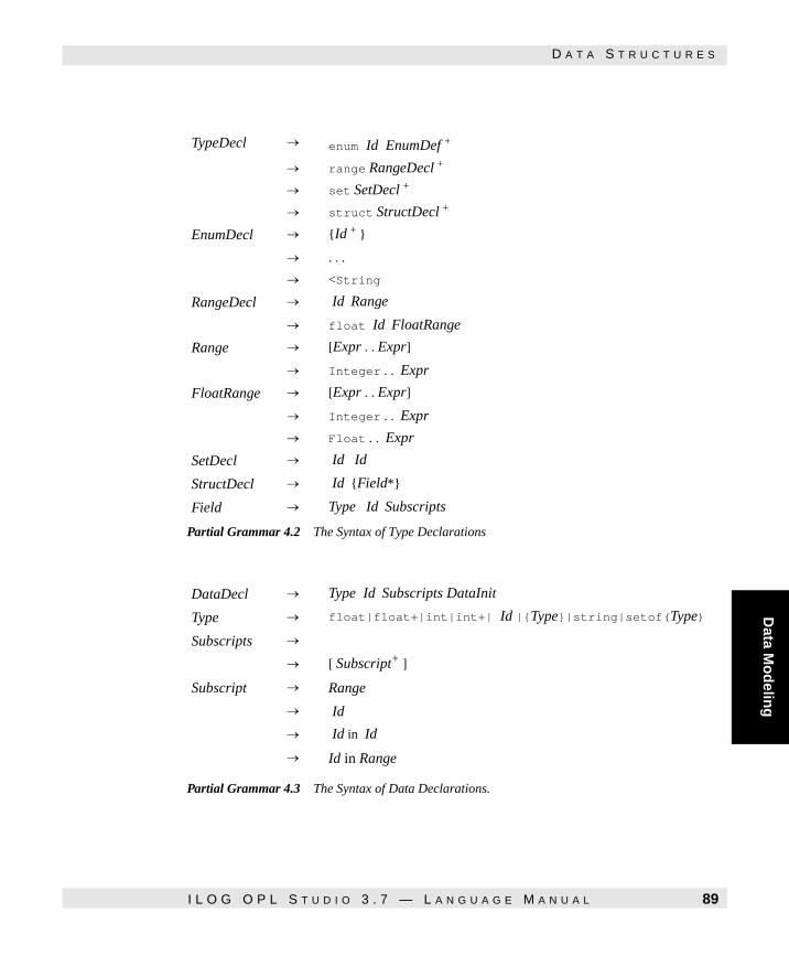
Data M
od
eling
D A T A S T R U C T U R E S
Partial Grammar 4.2
Partial Grammar 4.2 The Syntax of Type Declarations
Partial Grammar 4.3
Partial Grammar 4.3 The Syntax of Data Declarations.
TypeDecl → enum Id EnumDef +
→ range RangeDecl +
→ set SetDecl +
→ struct StructDecl +
EnumDecl → {Id + }
→ . . .
→ <String
RangeDecl → Id Range
→ float Id FloatRange
Range → [Expr . . Expr]
→ Integer . . Expr
FloatRange → [Expr . . Expr]
→ Integer . . Expr
→ Float . . Expr
SetDecl → Id Id
StructDecl → Id {Field*}
Field → Type Id Subscripts
DataDecl → Type Id Subscripts DataInit
Type → float|float+|int|int+| Id |{Type}|string|setof(Type)
Subscripts →
→ [ Subscript+ ]
Subscript → Range
→ Id
→ Id in Id
→ Id in Range
I L O G O P L S T U D I O 3 . 7 — L A N G U A G E M A N U A L 89
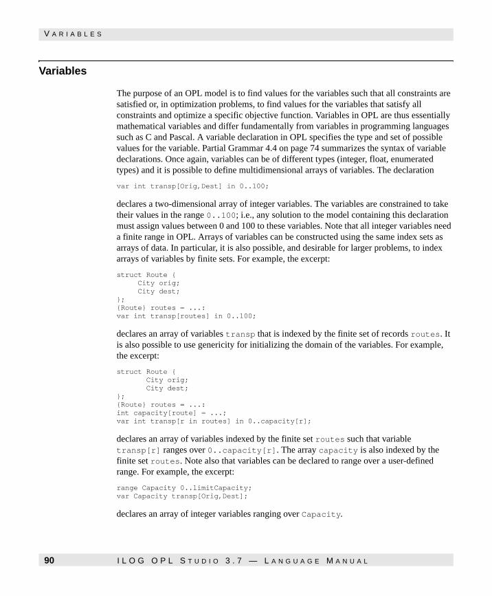
V A R I A B L E S
Variables
The purpose of an OPL model is to find values for the variables such that all constraints are satisfied or, in optimization problems, to find values for the variables that satisfy all constraints and optimize a specific objective function. Variables in OPL are thus essentially mathematical variables and differ fundamentally from variables in programming languages such as C and Pascal. A variable declaration in OPL specifies the type and set of possible values for the variable. Partial Grammar 4.4 on page 74 summarizes the syntax of variable declarations. Once again, variables can be of different types (integer, float, enumerated types) and it is possible to define multidimensional arrays of variables. The declaration
var int transp[Orig,Dest] in 0..100;
declares a two-dimensional array of integer variables. The variables are constrained to take their values in the range 0..100; i.e., any solution to the model containing this declaration must assign values between 0 and 100 to these variables. Note that all integer variables need a finite range in OPL. Arrays of variables can be constructed using the same index sets as arrays of data. In particular, it is also possible, and desirable for larger problems, to index arrays of variables by finite sets. For example, the excerpt:
struct Route { City orig; City dest; }; {Route} routes = ...: var int transp[routes] in 0..100;
declares an array of variables transp that is indexed by the finite set of records routes. It is also possible to use genericity for initializing the domain of the variables. For example, the excerpt:
struct Route { City orig; City dest; }; {Route} routes = ...: int capacity[route] = ...; var int transp[r in routes] in 0..capacity[r];
declares an array of variables indexed by the finite set routes such that variable transp[r] ranges over 0..capacity[r]. The array capacity is also indexed by the finite set routes. Note also that variables can be declared to range over a user-defined range. For example, the excerpt:
range Capacity 0..limitCapacity; var Capacity transp[Orig,Dest];
declares an array of integer variables ranging over Capacity.
90 I L O G O P L S T U D I O 3 . 7 — L A N G U A G E M A N U A L

Data M
od
eling
D A T A T Y P E S F O R S C H E D U L I N G A P P L I C A T I O N S
Variables can of course be declared individually, as in:
var int averageDelay in 0..maxDelay;
As mentioned previously, variables can be of different types. The excerpt:
var float+ transp[orig, dest];
declares a two-dimensional array of float variables that are constrained to be non-negative (i.e. their range is 0..∞). Float variables can be assigned more specific ranges, as in
var float+ transp[o in Orig, d in Dest] in 0..cap[o,d];
which declares a two-dimensional array of float variables, where variable transp[o,d] ranges over the set 0..cap[o,d]. This last declaration is of course equivalent to the declaration
var float transp[o in Orig, d in Dest] in 0..cap[o,d];
Variables over enumerated types are also useful for a variety of applications. The excerpt
enum Men ...; enum Women ...: var Women wife[Men];
declares an array wife of variables, indexed by the enumerated type Men and of type Women. Every solution to the model containing this excerpt assigns an element of Women to each variable in the array wife.
Data Types for Scheduling Applications
OPL also provides a number of data types tailored for scheduling applications. These data types represent important abstractions in modeling scheduling problems and OPL exploits them in special-purpose constraint-solving algorithms. The syntax of scheduling declarations is given in Partial Grammar 4.5 on page 76.
I L O G O P L S T U D I O 3 . 7 — L A N G U A G E M A N U A L 91

D A T A T Y P E S F O R S C H E D U L I N G A P P L I C A T I O N S
Partial Grammar 4.4
Partial Grammar 4.4 The Syntax of Variable Declarations
Origin and Horizon
All scheduling concepts used in OPL are defined over a global time interval
[scheduleOrigin; scheduleHorizon)
closed on the left and open on the right, like all time intervals in OPL. OPL has a default value for both the origin (0) and the horizon (a large number). However, it is recommended that they be specified for particular applications, since smaller time intervals make OPL more space- and time-efficient. The global origin and horizon can be specified by using instructions of the form
scheduleOrigin = 0; scheduleHorizon = 365;
It is of course possible to use expressions to initialize these values, as in
scheduleHorizon = sum(t in Tasks) duration[t];
Note that the declarations of scheduleOrigin and scheduleHorizon, if present, must come before the declarations of any other scheduling objects in the model. This is consistent with our convention of requiring that each object be used only after it is defined.
Activities
Probably the most fundamental concept in OPL for scheduling applications is the activity. An activity can be thought of as an object containing three data items, a starting date, a duration, and an ending date, together with the duration constraint that the ending date is the starting date plus the duration. In many applications, the duration of an activity is known and the activity is declared together with its duration, as in:
Activity carpentry(10);
VarDecl → var = VarDeclSfx+
VarDeclSfx → Id Id Subscripts
→ int Id Subscripts in Expr.. Expr
→ int+ Id Subscripts in Expr.. Expr
→ float Id Subscripts
→ float Id Subscripts in Expr.. Expr
→ float+ Id Subscripts
→ float+ Id Subscripts in Expr.. Expr
92 I L O G O P L S T U D I O 3 . 7 — L A N G U A G E M A N U A L

Data M
od
eling
D A T A T Y P E S F O R S C H E D U L I N G A P P L I C A T I O N S
which declares an activity carpentry whose duration is 10. The starting and ending dates of carpentry are integer variables taking their values in the global time interval and consistent with the duration constraint.
Activities can also be given a variable duration, in which case one commonly declares the task with an integer variable representing the duration, as in
var int durationCarpentry in 8..10; Activity carpentry(durationCarpentry);
which declares an activity carpentry whose duration is between 8 and 10. The duration variable durationCarpentry can appear in the problem constraints and the possible values for duration may thus be further constrained. It is also possible to declare an activity without specifying its duration, as in
Activity carpentry;
in which case the duration is an integer variable ranging over the interval
[0; scheduleHorizon - scheduleOrigin]
Arrays of activities can be declared in the visual way and the durations may be specified as described previously. For example, it is usual to declare an array of activities as follows:
Activity tasks [t in 1..10] (duration[t]);
The statement declares an array of 10 activities whose durations are duration[1],...,duration[10] respectively. The starting date, the duration, and the ending date of an activity are accessed in the way as the fields of a structure. For instance, carpentry.start, carpentry.end, and carpentry.duration represent the starting date, the ending date, and the duration of activity carpentry.
When modeling real applications, it may be important to recognize periods, such as weekends, when no activity can be scheduled. In OPL, these periods are called breaks. OPL provides several tools to specify breaks; these are discussed in Chapter 5, Expressions and Constraints. Some activities can be interrupted by breaks, while others cannot. In OPL, activities that can be interrupted by breaks are called breakable activities: they can start before a break and be resumed after a break. Activities in OPL are assumed to be unbreakable unless specified otherwise. The declaration:
Activity a breakable;
specifies that a is a breakable activity. Of course, breakable activities behave very much like other activities: they have a starting date, an ending date, and a duration, and they may require resources like activities. Their only added functionality is the ability to be interrupted by breaks. It is possible to declare arrays of breakable activities. For instance, the declaration:
Activity tasks[t in 1..10](duration[t]) breakable;
I L O G O P L S T U D I O 3 . 7 — L A N G U A G E M A N U A L 93
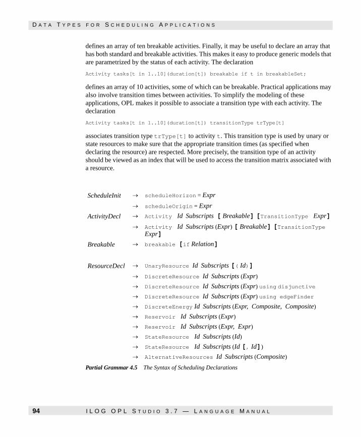
D A T A T Y P E S F O R S C H E D U L I N G A P P L I C A T I O N S
defines an array of ten breakable activities. Finally, it may be useful to declare an array that has both standard and breakable activities. This makes it easy to produce generic models that are parametrized by the status of each activity. The declaration
Activity tasks[t in 1..10](duration[t]) breakable if t in breakableSet;
defines an array of 10 activities, some of which can be breakable. Practical applications may also involve transition times between activities. To simplify the modeling of these applications, OPL makes it possible to associate a transition type with each activity. The declaration
Activity tasks[t in 1..10](duration[t]) transitionType trType[t]
associates transition type trType[t] to activity t. This transition type is used by unary or state resources to make sure that the appropriate transition times (as specified when declaring the resource) are respected. More precisely, the transition type of an activity should be viewed as an index that will be used to access the transition matrix associated with a resource.
Partial Grammar 4.5
Partial Grammar 4.5 The Syntax of Scheduling Declarations
ScheduleInit → scheduleHorizon = Expr
→ scheduleOrigin = Expr
ActivityDecl → Activity Id Subscripts [ Breakable] [TransitionType Expr]
→ Activity Id Subscripts (Expr) [ Breakable] [TransitionType Expr]
Breakable → breakable [if Relation]
ResourceDecl → UnaryResource Id Subscripts [( Id)]
→ DiscreteResource Id Subscripts (Expr)
→ DiscreteResource Id Subscripts (Expr) using disjunctive
→ DiscreteResource Id Subscripts (Expr) using edgeFinder
→ DiscreteEnergy Id Subscripts (Expr, Composite, Composite)
→ Reservoir Id Subscripts (Expr)
→ Reservoir Id Subscripts (Expr, Expr)
→ StateResource Id Subscripts (Id)
→ StateResource Id Subscripts (Id [, Id])
→ AlternativeResources Id Subscripts (Composite)
94 I L O G O P L S T U D I O 3 . 7 — L A N G U A G E M A N U A L

Data M
od
eling
D A T A T Y P E S F O R S C H E D U L I N G A P P L I C A T I O N S
Resources
Resources are a fundamental concept in scheduling applications and it is thus not surprising to find them as basic data types in OPL. OPL in fact supports a variety of resources, including unary, discrete, and discrete energy resources, as well as reservoirs.
Unary Resources
A unary resource is a resource that cannot be shared by two activities: i.e., as soon as an activity requires the resource, no other activities can make use of that resource. Unary resources are often used to model machines in job-shop scheduling or individual resources in resource-allocation problems. Activities generally require one or several unary resources during their execution. For instance, a job may require both a machine and an operator, both of whom can be modeled by unary resources. Unary resources are declared in OPL as
UnaryResource crane;
As usual, it is possible to declare arrays of unary resources, as in
UnaryResource machines[1..10];
which declares an array of 10 unary resources. It is also possible to associate a transition matrix with unary resources. The declaration
int m[TrType,TrType] = ...; UnaryResource machines[1..10](m);
associates a transition matrix m for the (user-defined) transition type TrType. Obviously, activities using this machine must use a transition type in TrType; an execution error is raised otherwise. More precisely, the transition types of two successive activities on a machine m[i] are used to index matrix m to obtain their transition times.
Discrete Resource
Discrete resources are another fundamental concept offered by OPL for scheduling applications. They are used to model resources that are available in multiple units, all units being considered equivalent and interchangeable as far as the application is concerned. For instance, a discrete resource may be used to model a budget or a pool of identical tools. Activities can then consume the discrete resource (e.g., spend part of the budget) or can require the resource during their execution (e.g., an activity can require a hammer) and return it to the pool upon completion. Discrete resources are declared in OPL by specifying their capacity, as in
DiscreteResource budget(30000);
which specifies that budget is a resource of capacity 30,000, i.e., there is $30,000 available. Of course, it is possible in OPL to declare arrays of discrete resources, as in
DiscreteResource res[t in 1..10](cap[t]);
I L O G O P L S T U D I O 3 . 7 — L A N G U A G E M A N U A L 95

D A T A T Y P E S F O R S C H E D U L I N G A P P L I C A T I O N S
which declares an array of 10 resources, the capacity of resource t being cap[t]. Note the generic way of specifying the capacity of the discrete resources. If all the discrete resources have the same capacity, say 3, then the declaration
DiscreteResource res[1..10](3);
is perfectly appropriate. A unary resource is a discrete resource of capacity 1 but the algorithms for unary resources are optimized to exploit all properties of this special case.
Discrete Energy Resources
It is often important in practical applications to obtain a precise schedule for the short-term, a rougher schedule for the medium-term, and a coarser schedule for the long term. For instance, one may be interested in a daily schedule for the first six months, a weekly schedule for the next six months, and a monthly schedule for the next year. Discrete energy resources are a generalization of discrete resource to support scheduling under such varying granularities. A discrete energy resource is declared by specifying its capacity and by specifying the time steps for the various successive time intervals. Consider for instance a problem where two workers must be assigned to some tasks and assume that we are interested in a schedule whose time steps are a day for the first week (a week is considered to consist of five days), two days for the next two weeks, and a week for the remaining of the schedule. A discrete energy resource of the form
int step[1..2] = [1,2,5]; int time[1..5] = [scheduleOrigin,5,15,scheduleHorizon]; DiscreteEnergy workers(2,step,time);
can be used for that purpose. It specifies that workers is a discrete energy resource of capacity two, with a time step of 1 for the interval [scheduleOrigin,5), a time step of 2 for the interval [5,15), and a time step of 5 days for the rest of the schedule. It is also interesting to consider what would be a legal schedule for the second and third week. Here the time step is 2 days and of course there are two workers available for each day. Hence, for every two successive days, the total "energy" available is 4 workers and, as a consequence, any solution can only schedule, over these two days, activities whose total capacity demand does not exceed 4. Note that only the total demand over the two days is constrained; for instance, there may be three activities (of duration one) requesting a worker on day 5 and one activity requesting a worker on day 6. More generally, on the above example, the total energy is 2 for each interval [t,t+1) in [0,5), 4 for each interval [t,t+2) in [5,15), and 10 for each interval [t,t+5) in the rest of the schedule and the activities scheduled in these intervals must satisfy the appropriate energy constraints.
Reservoirs
Unary and discrete resources are appropriate modeling tools when activities only require or consume resources. Some applications, however, may have a combination of activities, some of which require resources and others of which provide resources. For instance, an activity may require 10 gallons of oil, while another activity may supply oil at some point in time.
96 I L O G O P L S T U D I O 3 . 7 — L A N G U A G E M A N U A L

Data M
od
eling
D A T A T Y P E S F O R S C H E D U L I N G A P P L I C A T I O N S
Resources that can be required (consumed) and provided (produced) are called reservoirs in OPL. Reservoirs are declared, as in
Reservoir tank1(1000); Reservoir tank2(1000,100);
which declares a reservoir tank1 whose maximum capacity is 1,000 and initial capacity is 0 and a reservoir tank2 with the same maximum capacity but with an initial capacity of 100. As usual, it is possible in OPL to declare arrays of reservoirs.
State Resources
OPL also supports state resources, i.e., resources that are specified by a set of possible states. At any time in the schedule, a state resource is in a given state but that state may vary over time. For instance, an oven in a bakery may be modeled in terms of three states: hot, warm, and cold. At any time, the oven must be in one of these states but the oven may be warm at time 10 and hot at time 20. The excerpt
enum States { hot, warm, cold }; StateResource oven(States);
declares such a resource. Activities may require a resource to be in a given state (or a set of states) during their execution. The state of a state resource is an enumerated type or a range. As was the case with unary resources, it is also possible to declare a transition matrix for state resources by adding an argument after the set of states as in
enum States { hot, warm, cold }; int tm[States,States] = ...; StateResource oven(States,tm);
Alternative Resources
In many applications, an activity may require one of several resources, that are equivalent from the activity standpoint. However, the resources can sometimes not be equivalent from an application standpoint (e.g., some activities can only be performed by some of these resources). OPL supports these applications by providing the concept of alternative resources. Alternative resources are in fact sets of unary resources that can be declared, as in
UnaryResource oven[1..10]; AlternativeResources s(oven);
This declaration simply specifies that s is the set of unary resources oven[1],...,oven[10]. There is a fundamental difference between the above alternative resources and a discrete resource such as
DiscreteResource oven(10);
If the application is modeled with a discrete oven resource, a task may change ovens during its execution. The only requirement for discrete resources is that, at any time, there are enough ovens for all tasks requiring one. To the contrary, with alternative resources, the task is guaranteed to stay in the same oven during its execution. When permitted by the semantics of the application, it is preferable to use discrete resources rather than alternative resources,
I L O G O P L S T U D I O 3 . 7 — L A N G U A G E M A N U A L 97

C O N S T R A I N T D E C L A R A T I O N S
since the constraint-solving algorithms are more effective for discrete resources. The sections From Discrete to Unary Resources on page 268 and Alternative Resources on page 285 discuss this topic further.
Transition Time
OPL makes it possible to specify transition times between any two activities requiring the same unary and state resource. Given two activities a and b, the transition time between a and b is the amount of time that must elapse between the end of a and the beginning of b when a precedes b.
Partial Grammar 4.6
Partial Grammar 4.6 The Syntax of Constraint Declarations
Partial Grammar 4.7
Partial Grammar 4.7 The Syntax of Assertions
Transition times arise naturally in many scheduling applications, e.g., when tools must be set up on machines prior to the execution of a task. Typically, transition times also depend on the nature of the activities. If activities a and b use the same tools, the transition time may be small or nonexistent. If they use fundamentally different tools, the transition times may be larger. Transition times are specified in two steps in OPL. First, every activity involving transition times must be associated with a transition type (an integer or an enumerated value) that will be used to index a transition matrix. Second, the unary or state resource must be associated with a transition matrix that, given two transition types associated with two successive activities, returns a transition time.
Constraint Declarations
OPL also allows constraint declarations. This feature is useful in many problems for displaying constraints and analyzing the results of OPL, as well as for removing and restoring constraints in OPL Studio. The syntax of constraint declarations is shown in Partial Grammar 4.6. For instance, a declaration
constraint capCstr[Machines];
declares an array capCstr of constraints. Chapter 5, Expressions and Constraints describes how to initialize elements of this array.
ConstraintDecl → constraint (Id) (Subscript)
Assert → assert (Astr)
98 I L O G O P L S T U D I O 3 . 7 — L A N G U A G E M A N U A L
Data M
od
eling
D A T A C O N S I S T E N C Y
Data Consistency
OPL also provides assertions to verify the consistency of the model data. This functionality is often useful to avoid tedious model debugging or wrong results due to incorrect input data. These assertions are similar to the assert instruction in C. In their simplest form, assertions are simply Boolean expressions that must be true; they raise an execution error otherwise. For instance, it is common in some transportation problems to require that demand matches the supply. The declaration
{int} demand[Customers] = ...; {int} supply[Suppliers] = ...;
assert sum(s in Suppliers) supply[s] = sum(c in Customers) demand[c];
makes sure that the total supply of the suppliers meets the total demand of the customers. This assertion can be generalized to the case of multiple products, as in
{int} demand[Customers,Products] = ...; {int} supply[Suppliers,Products] = ...; assert forall(p in Products) sum(s in Suppliers) supply[s,p] = sum(c in Customers) demand[c,p];
which verifies that the total supply meets the total demand for each product. The use of assertions is highly recommended, since they make it possible to detect errors in the data input early, avoiding tedious inspection of the model data and results. Partial Grammar 4.7 on page 80 summarizes the syntax of assertions.
Initialization
As mentioned previously, there are various ways to initialize data in OPL:
◆ inline initialization: the initialization is given together along the declaration;
◆ offline initialization: the initialization is given subsequently in a data instruction or in a separate OPL Studio file;
◆ computed initialization: the initialization is given by an initialize instruction;
◆ file initialization: the initialization is given in a file.
◆ database initialization: the initialization is performed by reading from a database.
◆ spreadsheet initialization: the initialization is performed by reading from a spreadsheet.
Database initializations are discussed in Chapter 11, Databases and spreadsheet initializations are discussed in Chapter 12, Spreadsheets. The rest of this section discusses the other initializations.
I L O G O P L S T U D I O 3 . 7 — L A N G U A G E M A N U A L 99
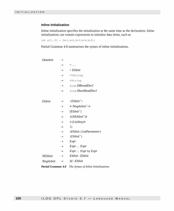
I N I T I A L I Z A T I O N
Inline Initialization
Inline initialization specifies the initialization at the same time as the declaration. Inline initializations can contain expressions to initialize data items, such as
int a[1..5] = [b+1,b+2,b+3,b+4,b+5];
Partial Grammar 4.8 summarizes the syntax of inline initializations.
Partial Grammar 4.8
Partial Grammar 4.8 The Syntax of Inline Initializations
DataInit →
→ = . . .
→ = EltInit
→ <<String
→ <String
→ from DBreadDecl
→ from SheetReadDecl
EltInit → <EltInit+>
→ #<NtupleInit+>#
→ [EltInit+]
→ #[NEltInit+]#
→ #{ListSeq}#
→ {}
→ {EltInit | ListParameter}
→ {EltInit+}
→ Expr
→ Expr ... Expr
→ Expr ... Expr by Expr
NEltInit → EltInit : EltInit
NtupleInit → Id : EltInit
100 I L O G O P L S T U D I O 3 . 7 — L A N G U A G E M A N U A L
Data M
od
eling
I N I T I A L I Z A T I O N
Offline Initialization
Offline initialization specifies the initialization of a data item in a data instruction. The fact that the data is initialized in a data instruction is specified using = ... in the declaration. This functionality makes it possible to have model and data files in OPL Studio, each data file corresponding in fact to a data instruction. For instance, the excerpt
int a[1..2] = ...; int b[1..3] = ...; ...data { b = [1 2 3]; a = [3,4]; };
declares two arrays whose initializations are given in the data instruction. Note that the order of the initializations in the data instruction is not significant and that commas can be omitted as separators in arrays, sets, and records. However, we stress that data instructions cannot contain expressions, since they are intended to specify data. The data instruction also makes it possible to specify sets of records in very compact ways. Consider the types
enum Product {flour, wheat, sugar}; enum City {Providence, Boston, Mansfield}; struct Ship { City orig: City dest; Product p: };
and assume that a set of shipments must be initialized with the values
<Providence, Boston, wheat>; <Providence, Boston, flour>; <Providence, Boston, sugar>; <Providence, Mansfield, wheat>; <Providence, Mansfield, flour>; <Boston, Providence, sugar>; <Boston, Providence, flour>;
The OPL declaration
{Ship} shipment = #{ <Providence> :: {<Boston> :: {<wheat> <flour> <sugar>} <Mansfield> :: {<wheat> <flour>}} <Boston> :: {<Providence> :: {<sugar> <flour>}} }#;
factors redundancies across the tuples. The compact form is enclosed in #{ and }# instead of {and}. In addition, it uses a concatenation operator r :: S that, given a tuple r and a set of tuples S = {r1,...,rn}, returns the set of records r’1,...,r’n , where ri is the concatenation of the tuple r and ri . Partial Grammar 4.8 on page 100 summarizes the syntax of offline initializations.
I L O G O P L S T U D I O 3 . 7 — L A N G U A G E M A N U A L 101

I N I T I A L I Z A T I O N
Partial Grammar 4.9
Partial Grammar 4.9 The Syntax of Offline Initializations
Data → data {{ListInit}};
InitStatement → Id = Define;
Define → Integer
→ Float
→ Id
→ <ListDefine>
→ #<ListNTDefine>#
→ {ListDefine}
→ [ListDefine]
→ #[ListNTDefine]#
→ #{ListSeq}#
ListDefine →
→ Define ListDefine
→ Define, ListDefine
NDefine → Define : Define
ListNDefine →
→ NDefine ListNDefine
→ NDefine, ListNDefine
NTDefine → Id : Define
ListNTDefine →
→ NTDefine ListNTDefine
→ NTDefine, ListNTDefine
ListSeq → ListSeqo| ListSeqn
ListSeqo → Seqo
→ Seqo ListSeqo
→ ListSeqo, ListSeqo
Seqo → <ListDefine>
→ <ListDefine>::{ListSeqo}
ListSeqn → Seqn
→ Seqn ListSeqn
→ Seqn, ListSeqn
Seqn → #<ListNTDefine>#
→ #<ListNTDefine>#::{ListSeqn}
102 I L O G O P L S T U D I O 3 . 7 — L A N G U A G E M A N U A L

Data M
od
eling
I N I T I A L I Z A T I O N
Computed Initializations
Computed initializations are often useful to transform data stored in some format into a form more appropriate to state the model effectively. Consider a transportation problem in which the input data is given by a list of tuples of the form
<orig,dest,c>
This indicates that there is a route between cities orig and dest with a shipment cost c. For instance, the input data can be described by the instructions
struct InputData { City orig; City dest; float c; }; {InputData} inData = ...:
It may be useful in the model to have an array cost declared as follows:
struct Route { City orig; City dest; }; {Route} routes = {<orig,dest> | <orig,dest,c> in inData}; float+ cost[routes];
This array can be initialized by the initialize instruction
forall(d in inData) cost[<d.orig,d.dest>] = d.cost;
or, equivalently, using tuples as
initialize forall(<o,d,c> in inData) cost[<o,d>] = c;
initialize instructions can have several parts, as in
{int} a[0..9]; {int} odd = {1, 3, 5, 7, 9}; {int} even = {2, 4, 6, 8, 10};
initialize { forall(i in 0..5) a[i] = odd; forall(i in 6..9) a[i] = even; };
I L O G O P L S T U D I O 3 . 7 — L A N G U A G E M A N U A L 103

I N I T I A L I Z A T I O N
Partial Grammar 4.10 summarizes the syntax of computed initializations.
Partial Grammar 4.10
Partial Grammar 4.10 The Syntax of Computed Initializations
File Initializations
The last type of initialization involves listing the values of a data item in a file. For instance, the declaration
struct Prec { int id; Task before; Task after; }; {Prec} precedences < "prec.txt";
declares a set of records precedences whose initialization is given in the file prec.txt. The file prec.txt simply lists without punctuation all the values necessary to initialize precedences. For instance, the file prec.txt may contain the values
1 a1 a2 2 a2 a3 3 a3 a4 4 a4 a5
Note that the data need not be given on a single line. The file prec.txt may be organized as:
1 a1 a2 2 a2 a3 3 a3 a4 4 a4 a5
Of course, OPL makes sure that the types of the values correspond to their declarations and that enough values are provided. Arrays can be initialized in the same fashion, e.g.
int array [1..10] < "arr.txt";
The file arr.txt may contain, for instance, the values
3 4 5 6 7 10 11 12 13 14
Initialize → Initialize (InitBody)
(InitBody) → Expr = Expr
→ forall (ListParameter) InitBody
→ if Relation then InitBody endif
→ if Relation then InitBody else InitBody endif
→ {InitBody}
→
104 I L O G O P L S T U D I O 3 . 7 — L A N G U A G E M A N U A L
Data M
od
eling
I N I T I A L I Z A T I O N
The only case in which punctuation symbols are needed in file initializations is when a set type is used inside another data structure. For instance, given the declaration
{int} a[1..3] < "a.txt";
the file a.txt may contain, for instance,
{3 4 5 6 7}{3 4 6 7 8}{2 3 4 5 9}
The braces are needed here to determine when the description of the set is completed. It is useful to stress that the file initialization is more memory-efficient than online or offline initialization and should be used for very large files.
Debugging Data
It is often desirable to be able to browse through the data before actually running a model, e.g., to check its validity or to observe its structure. Here is a simple way to this in OPL: simply use an empty set of constraints as in
solve;
OPL Studio will then let you browse through your data using graphical representation whenever possible.
I L O G O P L S T U D I O 3 . 7 — L A N G U A G E M A N U A L 105

I N I T I A L I Z A T I O N
106 I L O G O P L S T U D I O 3 . 7 — L A N G U A G E M A N U A L

C H A P T E R
Exp
ression
and
C
on
straints
5
Expressions and Constraints
This chapter describes expressions, relations, and constraints in OPL. Before proceeding further, it is important to recognize that expressions and relations are used in two fundamentally different ways in OPL:
◆ to specify and initialize data
◆ to state constraints over variables.
In the first case, the expressions and relations do not contain variables or activities, since these variables have no value at this stage of the computation. These expressions and relations are said to be ground and they are subject to almost no restrictions. In the second case, of course, the expressions and relations may contain variables (and/or activities). Relations containing variables and activities are called constraints and are subject to a number of restrictions (e.g., float constraints must be linear or piecewise-linear).
You can find information on the following topics:
◆ Expressions and Relations on page 108 describes expressions and relations in a general way, i.e., without concern for the restrictions imposed on constraints.
◆ Constraints on page 121 presents the general constraints allowed in OPL.
◆ Stating Constraints on page 134 discusses the tools offered in OPL to state constraints.
I L O G O P L S T U D I O 3 . 7 — L A N G U A G E M A N U A L 107

E X P R E S S I O N S A N D R E L A T I O N S
Expressions and Relations
This section reviews how expressions and relations are built. Restrictions imposed on constraints are discussed in the section Constraints on page 121.
Data and Variable Identifiers
Since data and variable identifiers are the basic components of expressions, it is useful to review briefly how they are used to build expressions. If r is a record with a field capacity of type T, then r.capacity is an expression of type T. If a is a n-dimensional array of type T, a[e1,...,en] is an expression of type T, provided that ei are well-typed. For instance, the excerpt
int limit[routes] = ...; var int transp[r in routes] in 0..limit[r];
contains an expression limit[r] of type integer. Indices of arrays can be complex expressions. For instance, the excerpt
int nbFlights = ...; range Flight 1..nbFlights; enum Employee ...: var int crew[Flight , Employee] in 0..1; solve { ... forall(e in Employee) forall(i in 1..nbFlights - 2) crew[i,e] + crew[i+1,e] + crew[i+2,e] >= 1; };
contains an integer expression crew[i+1,e] whose first index is itself an integer expression. The excerpt
forall(w in Women) forall(i in R) rankWomen[w,favoriteMen[w,i]] = i;
contains an expression favoriteMen[w,i] as the second index of array rankWomen. Indices of arrays can also contain variables.
For instance, the excerpt
range Warehouses ...; range Customers ...; var Warehouses supplier[Customers]: var int open[Customers] in 0..1; solve { ... forall(c in Customers) open[supplier[c]] = 1; }
108 I L O G O P L S T U D I O 3 . 7 — L A N G U A G E M A N U A L

Exp
ression
and
C
on
straints
E X P R E S S I O N S A N D R E L A T I O N S
contains an expression Open[supplier[c]] and supplier[c] is an integer variable. The ability to use variables in indices makes possible some very compact models for some combinatorial optimization problems.
Integer Expressions
Integer expressions are constructed from integer constants, integer data, integer variables, and the traditional integer operators such as +, -, *, /, mod; the operator / represents integer division (e.g., 8/3 = 2) and the operator mod represents integer remainder. OPL also supports the operator abs, which returns the absolute value of its argument, and the constant maxint, which represents the largest integer representable in OPL. Users should, of course, be aware that expressions involving large integers may produce overflow.
Float Expressions
Table 5.1 Float Functions in OPL
Function Type Semantics
abs(float f) float the absolute value of f
ceil(float f) float the smallest integer grater or equal to f
distToInt(float f) float the distance from f to the nearest integer
exp(float f) float ef
floor(float f) float the largest integer smaller or equal to f
frac(float f) float the fractional part of f
ftoi(float f) int the integer represented by f
lg(float f) float base 2 logarithm of f
ln(float f) float natural logarithm of f
log(float f) float base 10 logarithm of f
nearest(float f) float the nearest integer to f
pow(float x, float y) float xy
sqrt(float f) float the square root of f
trunc(float f) float the integer part of f
I L O G O P L S T U D I O 3 . 7 — L A N G U A G E M A N U A L 109

E X P R E S S I O N S A N D R E L A T I O N S
Float expressions are constructed from floats, float data and variables, as well as operations such as +, -, /, *. In addition, OPL contains a float constant infinity to represent ∞ and a variety of operations depicted in Table 5.1 on page 109.
Note that nearest(f) returns ceil(a) when frac(a)=0.5. In other words nearest(0.5) returns the value 1. Integers and floats can be mixed inside the same expressions: integers are automatically converted to type float in such expressions. Note that the results of all these float functions are of type float. The function ftoi (float to integer) can be used to convert an integer represented as float into an integer represented as an integer. For instance, the declaration
int i = ftoi(nearest(4.7));
is valid, while the declaration
int i = nearest(4.7);
produces a semantic error. The result of function ftoi is undefined when the integer cannot be represented exactly in type int.
The pow function accepts integer variables and constants as well as float variables and constants for x and y in x = pow(y,e).
Enumerated Expressions
Enumerated expressions are constructed from enumerated values, enumerated data and variables, as well as a number of functions over enumerated types and values. OPL supports various functions over enumerated types. The function first and last, when applied to an enumerated type T, returns the first and the last enumerated values of T. For instance, the excerpt
enum Days { Monday, Tuesday, Wednesday, Thursday, Friday, Saturday, Sunday };Days f = first(Days); Days l = last(Days);
initializes f and l to Monday and Sunday respectively. This also indicates that enumerated sets (and, in fact, all sets) in OPL are totally ordered according to their order of appearance in the initialization. The function card, when applied to an enumerated type, returns the number of enumerated values in the type. For instance, card(Days) returns 7. A number of functions are also available on enumerated values. Function ord(v) returns the position of value v in the enumerated type, with the understanding that positions start at zero (as in C and Pascal). For instance, ord(Tuesday) = 1 and ord(Sunday) = 6. The function next(v) returns the successor to v if it exists and raises an error otherwise (e.g., next(Monday) = Tuesday) and function prev(v) returns the predecessor to v if it exists and raises an error otherwise (e.g., prev(Tuesday) = Monday). These functions can be generalized to give the ith successor (respectively predecessor) of a value (i ≥ 0). For instance, next(Monday,3) = Thursday. Once again, this value should be well-defined or an execution error is produced. OPL also supports circular versions of these functions (i.e.,
110 I L O G O P L S T U D I O 3 . 7 — L A N G U A G E M A N U A L

Exp
ression
and
C
on
straints
E X P R E S S I O N S A N D R E L A T I O N S
nextc and prevc) which consider that the successor of the last element of the type is the first element and vice-versa for the predecessor. For instance, nextc(Sunday) = Monday, while next(Sunday) raises an error. Enumerated expressions can be used as indices or indexed by other enumerated expressions. For instance, the excerpt
enum Men ...; enum Women ...; var Women wife[Men]; var Men husband[Women]; ... solve { ... forall(m in Men) husband[wife[m]] = m; ... };
is an enumerated expression husband[wife[m]] where the enumerated array husband is indexed by another enumerated expression wife[m]. Note that, in this example, husband and wife are both arrays of variables.
Aggregate Operators
Integer and float expressions can also be constructed using aggregate operators for computing summations (sum), products (prod), minima (min), and maxima (max) of a collection of related expressions. For instance, the excerpt
int capacity[Routes] = ...; int minCap = min(r in Routes) capacity[r];
uses the aggregate operator min to compute the minimum value in array capacity. The form of the formal parameters in these aggregate operators is very general and is discussed at length in Chapter 6, Formal Parameters.
In addition to the sum, prod, min and max aggregates, OPL also supports a conjunctive and a disjunctive aggregate called respectively and and or. Both share with all the other aggregates the same syntax for the specification of their formal arguments which is discussed at length in Chapter 6, Formal Parameters.
For instance, the excerpt
var int x[i in 1..5] in 1..5; solve { and(i in 1..5) (x[i]=i); };
constrains each variable x[i] to equal i and is equivalent to
x[1]=1 & x[2]=2 & x[3]=3 & x[4]=4 & x[5]=5
I L O G O P L S T U D I O 3 . 7 — L A N G U A G E M A N U A L 111

E X P R E S S I O N S A N D R E L A T I O N S
while the statement
var int x[i in 1..5] in 1..5; solve { or(i in 1..5) (x[i]=i); };
states that at least one of the variables in the array x should be bound to its index value.
As an alternative, you can use the minl and maxl operators on a list of expressions separated by a comma. For example:
int maximum = maxl (a[1],17,b[12]);
Conditional Expressions
It is often useful to use conditional expressions as part of larger expressions. OPL makes this possible through a general case expression. Consider the instructions
int c = ...; int a = case { c = 1 -> 2; c = 2 -> 5; 8 };
The expression case { c = 1 -> 2; c = 2 -> 5; 8 } returns the value 2 to a if c is 1, 5 if c is 2, and 8 otherwise. Conditional statements of this form should return integers or floats. Note also that these expressions can be embedded in more complex expressions as in
int c = ...; int a = 5 * case { c = 1 -> 2; c = 2 -> 5; 8 };
Piecewise Linear Functions
OPL also supports piecewise-linear functions, which are important in many applications. Piecewise-linear functions are discussed at length in Chapter 13, Linear and Integer Programming. Piecewise-linear functions are often specified by giving a set of slopes, a set of breakpoints at which the slopes change, and the value of the functions at a given point. Consider, for instance, a transportation problem in which the transportation cost ship[o,d] between two locations o and d depends on the size of the shipment. The piecewise-linear expression
piecewise{10 -> 100;20 -> 200;40}(0,0) ship[o,d];
describes the piecewise-linear function of ship[o,d] depicted in Figure 5.1. The function has slopes 10, 20, and 40, breakpoints 100 and 200, and evaluates to 0 at point 0.
112 I L O G O P L S T U D I O 3 . 7 — L A N G U A G E M A N U A L

Exp
ression
and
C
on
straints
E X P R E S S I O N S A N D R E L A T I O N S
Figure 5.1
Figure 5.1 A Piecewise-Linear Function.
In other words, the piecewise-linear expression is equivalent to the expression:
10 * ship[o,d]
when ship[o,d] <= 100, to
10 * 100 + 20 * (ship[o,d] - 100)
when 100 <= ship[o,d] <= 200 and to
10 * 100 + 20 * 100 + 40 * (ship[o,d] - 200)
otherwise.
By default, OPL assumes that a piecewise-linear function evaluates to zero at the origin, so that the above piecewise-linear function could actually be written as
piecewise{10 -> 100;20 -> 200;40} ship[o,d];
The above piecewise-linear function has a fixed number of pieces, but OPL also allows generic pieces. The number of pieces may then depend on the input data, as in
piecewise { forall(i in 1..n) slope[i] -> breakpoint[i]; slope[n+1]; } ship[o,d];
This piecewise-linear function is equivalent to
slope[1] * ship[o,d]
when ship[o,d] <= breakpoint[1] to
I L O G O P L S T U D I O 3 . 7 — L A N G U A G E M A N U A L 113

E X P R E S S I O N S A N D R E L A T I O N S
slope[1] * breakpoint[1] +
slope [i] * (breakpoint[i] - breakpoint[i-1] +
slope[k] * (ship[o,d] - breakpoint[k-1])
when
breakpoint[k-1] < ship[o,d] <= breakpoint [k] (1 ≤ k ≤ n )
and to
slope[1] * breakpoint[1] +
slope [i] * (breakpoint[i] - breakpoint[i-1] +
slope[n+1] * (ship[o,d] - breakpoint[n])
otherwise. Note that there may be several generic pieces in piecewise-linear functions. It is important to stress that breakpoints and slopes in piecewise-linear functions must always be ground and that the breakpoints must be strictly increasing. Chapter 13, Linear and Integer Programming, discusses piecewise-linear functions in more detail.
Set Expressions
Set data can be initialized by set expressions, as mentioned in Chapter 4, Data Modeling. These expressions are constructed from previously defined sets and the set operations union, inter, diff, and symdiff. For instance,
{int} s1 = {1,2,3}; {int} s2 = {1,4,5}; {int} i = s1 inter s2; {int} u = s1 union s2; {int} d = s1 diff s2; {int} sd = s1 symdiff s2;
initializes i to {1}, u to {1,2,3,4,5}, d to {2,3}, and sd to {2,3,4,5}. Set expressions can also be constructed from some aggregate operators. For instance, the excerpt
{int} a[R] = ...; {int} U = union(s in R) a[s]; {int} i = inter(s in R) a[s];
illustrates how to compute the union and intersection of a collection of sets (note that the order of the elements in these sets is implementation-dependent). In addition, set expressions can be constructed from ranges. For instance, the excerpt
{int} s = 1..10; {int} ps = 1..10 by 2;
initializes s to the finite set {1,2,...,10} and ps to the finite set {1,3,5,7,9}. It is important to stress that the range 1...10 takes constant space, while the set s takes space proportional to the number of elements in the range.
k 1–i 2=∑
ni 2=∑
114 I L O G O P L S T U D I O 3 . 7 — L A N G U A G E M A N U A L
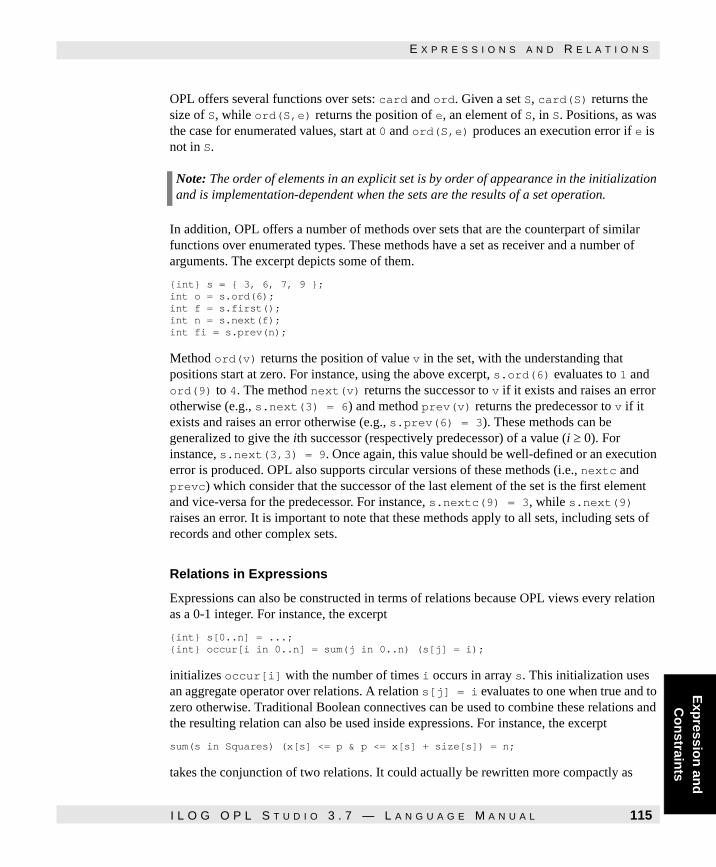
Exp
ression
and
C
on
straints
E X P R E S S I O N S A N D R E L A T I O N S
OPL offers several functions over sets: card and ord. Given a set S, card(S) returns the size of S, while ord(S,e) returns the position of e, an element of S, in S. Positions, as was the case for enumerated values, start at 0 and ord(S,e) produces an execution error if e is not in S.
In addition, OPL offers a number of methods over sets that are the counterpart of similar functions over enumerated types. These methods have a set as receiver and a number of arguments. The excerpt depicts some of them.
{int} s = { 3, 6, 7, 9 }; int o = s.ord(6); int f = s.first(); int n = s.next(f); int fi = s.prev(n);
Method ord(v) returns the position of value v in the set, with the understanding that positions start at zero. For instance, using the above excerpt, s.ord(6) evaluates to 1 and ord(9) to 4. The method next(v) returns the successor to v if it exists and raises an error otherwise (e.g., s.next(3) = 6) and method prev(v) returns the predecessor to v if it exists and raises an error otherwise (e.g., s.prev(6) = 3). These methods can be generalized to give the ith successor (respectively predecessor) of a value (i ≥ 0). For instance, s.next(3,3) = 9. Once again, this value should be well-defined or an execution error is produced. OPL also supports circular versions of these methods (i.e., nextc and prevc) which consider that the successor of the last element of the set is the first element and vice-versa for the predecessor. For instance, s.nextc(9) = 3, while s.next(9) raises an error. It is important to note that these methods apply to all sets, including sets of records and other complex sets.
Relations in Expressions
Expressions can also be constructed in terms of relations because OPL views every relation as a 0-1 integer. For instance, the excerpt
{int} s[0..n] = ...; {int} occur[i in 0..n] = sum(j in 0..n) (s[j] = i);
initializes occur[i] with the number of times i occurs in array s. This initialization uses an aggregate operator over relations. A relation s[j] = i evaluates to one when true and to zero otherwise. Traditional Boolean connectives can be used to combine these relations and the resulting relation can also be used inside expressions. For instance, the excerpt
sum(s in Squares) (x[s] <= p & p <= x[s] + size[s]) = n;
takes the conjunction of two relations. It could actually be rewritten more compactly as
Note: The order of elements in an explicit set is by order of appearance in the initialization and is implementation-dependent when the sets are the results of a set operation.
I L O G O P L S T U D I O 3 . 7 — L A N G U A G E M A N U A L 115

E X P R E S S I O N S A N D R E L A T I O N S
sum(s in Squares) (x[s] <= p <= x[s] + size[s]) = n;
Other connectives such as \/ (disjunction), not (negation), => (implication), and <=> (equivalence) can also be used.
Reflective Functions
Reflective functions are used to obtain information about the current state of the computation, e.g., the domains of the variables or the current value of a floating-point variable in the linear relaxation. Their arguments are in general variables. Table 5.2 on page 117 gives their signatures, preconditions, and semantics. To express the preconditions, we use e to indicate that the expression e must be ground and, in the semantics, we use dom(c) to represent the domain of c in the current computation state. UnaryResource and DiscreteResource can also be abbreviated by Unary and Discrete for compactness. Note that a signature of the form dmin(int c) specifies that dmin expects an argument of type integer but the argument may be a data or a variable (i.e., the signature constrains only the type). OPL also makes it is possible to use v.rc as an abbreviation of reducedCost(v).
Reflective functions should only be used to express heuristics and search procedures, since they are operational in nature and rely on the state of the variables at some execution step. As mentioned previously, one of the appealing features of constraint programming in general, and OPL in particular, is its declarative nature: statements can be given a meaning without relying on knowledge of how they are executed. However, the use of reflective functions outside the specification of heuristics jeopardizes this benefit.
Relations
Like expressions, relations can have various types in OPL. Integer relations are constructed from integer expressions and the traditional relational operators =, <> (not equal), >=, >, <, and <=. Float relations are constructed from float expressions and the same relational operators. Enumerated relations are constructed from enumerated expressions and support the same operators as well. Of course, only data from the same enumerated types can be compared. Finally, string relations are constructed from string expressions and support the same operators as well.
116 I L O G O P L S T U D I O 3 . 7 — L A N G U A G E M A N U A L

Exp
ression
and
C
on
straints
E X P R E S S I O N S A N D R E L A T I O N S
Table 5.2 Reflective Functions in OPL
Function Type Semantics
dmin(int c) int the minimum value in dom(c)
dmax(int c) int the maximum value in dom(c)
dmin(float c) float the minimum value in dom(c)
dmax(float c) float the maximum value in dom(c)
dsize(int c) int the size of dom(c)
dsize(enum c) int the size of dom(c)
dnexthigher(int c, int e) int the smallest value greater than e in dom(c)or e if none exists
dnextlower(int c, int e) int the largest value smaller that e in dom(c)
isInDomain(int x, int v) int 1 if v is dom(x) and 0 otherwise
regretdmin(int c) int dnexthigher(c,dmin(c)) - dmin(c)
regretdmax(int c) int dmax(c) - dnextlower(c,dmax(c))
simplexValue(int c) float the value of c in the simplex solution
simplexValue(float c) float the value of c in the simplex solution
reducedCost(int c) float the reduced cost of c in the simplex solution
reducedCost(float c) float the reduced cost of c in the simplex solution
bound(int c) int 1 if dmin (c) = dmax (c) and 0 otherwise
bound(enum c) int 1 if dsize (c) = 1 and 0 otherwise
bound(float c) int 1 if dmin (c) = dmax(c) and 0 otherwise
nbOccur(int e, [int] id) int the number of occurrences of e in array id
isRanked(Unary) int 1 if the resource is ranked and 0 otherwise
isRanked([Unary]) int 1 if all resources are ranked and 0 otherwise
nbPossibleFirst(Unary) int number of activities that can be ranked first
nbPossibleLast(Unary) int number of activities that can be ranked last
isPossibleFirst(Unary r, Activity a)
int true if a can potentially be ranked first on r
isPossibleLast(Unary,Activity) int true if a can potentially be ranked last on r
I L O G O P L S T U D I O 3 . 7 — L A N G U A G E M A N U A L 117

E X P R E S S I O N S A N D R E L A T I O N S
Relations can also be used in sequence, as shown before. For instance
low <= x <= up;
can be used instead of
low <= x; x <= up;
Similarly, a relation
a <= b <= c <= d;
can be used instead of
a <= b; b <= c; c <= d;
Note that
a <= b <= c;
is fundamentally different from
(a <= b) <= c;
This last constraint is a higher-order inequality between (a <= b) and c. Finally, note that a relation (a <= b <= c) has the same truth value as a <= b & b <= c.
OPL also supports the relations e in S and e not in S, where e has type T and S has type "set of T", to check membership and nonmembership in a set. Finally, as mentioned previously, relations can also be combined by the traditional logical connectives: negation (not), disjunction \/, conjunction &, implication =>, and equivalence <=>.
Syntax
Partial Grammar 5.1 and 5.2 describe the syntax of expressions and relations in OPL. In addition, Table 5.3 on page 121 specifies the precedence of the operators. OPL uses the conventions that higher numbers have precedence over lower ones, that expressions containing operators at the same level are parsed from left to right and top to bottom, and that parentheses can overwrite the order of evaluation. Note also that nested search
localSlack(Unary) int local slack of the resource
globalSlack(Unary) int global slack of the resource
localSlack(Discrete) int local slack of the resource
globalSlack(Discrete) int global slack of the resource
rand() int pseudo-random integer
rand(int m) int pseudo-random integer modulo m
Table 5.2 Reflective Functions in OPL (Continued)
118 I L O G O P L S T U D I O 3 . 7 — L A N G U A G E M A N U A L

Exp
ression
and
C
on
straints
E X P R E S S I O N S A N D R E L A T I O N S
expressions such as solve, minof, and maxof only make sense when used in the search procedure. C:Partial Grammar 0.1
Partial Grammar 5.1 The Syntax of Expressions
Expr → + Expr→ - Expr→ Expr Operator Expr→ AggregateOperator (ListParameter) Expr→ piecewise {ListPiece} Composite→ piecewise {ListPiece} (Expr, Expr) Composite→ (Relation)
→ (Expr)
→ Composite→ Integer
→ Float
→ infinity
→ maxint
→ solve (Search)
→ minof (Expr, Choice)
→ maxof (Expr, Choice)
→ case (Cases)
ListPiece → Expr→ Expr-> Expr; ListPiece→ forall (ListParameter) Expr-> Expr; ListPiece
Cases → { Relation -> Expr;} Expr
Composite → Id Dereference
Dereference → {Deref}
Deref → [Actuals]
→ . Id→ (Actuals)
Actuals → EltInit+
Operator → +|-|*|/|mod|union|diff|inter|symdiff
AggregateOperator → sum|min|max|union|prod|inter
I L O G O P L S T U D I O 3 . 7 — L A N G U A G E M A N U A L 119

E X P R E S S I O N S A N D R E L A T I O N S
Partial Grammar 5.2
Partial Grammar 5.2 The Syntax of Relations
Relation → Expr RelSfx+
→ Composite SchedOp Composite
→ Composite SchedOp ( Expr) Composite
→ not Relation
→ Relation LogicalOp Relation
→ Expr in Expr
→ Expr not in Expr
→ Expr subset Expr
→ Composite precedes Composite
→ activityHasSelectedResource ( Composite, Composite, Composite)
RelSfx → RelOp Expr
RelOp → =|>=|<=|>|<|<>
SchedOp → requires|consumes|provides|produces
LogicalOp → &|\/|=>|<=>
120 I L O G O P L S T U D I O 3 . 7 — L A N G U A G E M A N U A L

Exp
ression
and
C
on
straints
C O N S T R A I N T S
Constraints
Constraints are a subset of relations. This section specifies the constraints supported by OPL and discusses various subclasses of constraints to illustrate the rich support available for modeling combinatorial optimization applications. Partial Grammar 5.3 on page 122 summarizes the syntax of constraints in OPL.
Table 5.3 Operator Precedences.
Class Operator Precedence
Logical <=> 0
=> 1
\/ 2
& 3
not 4
Relational =, <=, >=, <, >, <> 5
in, not in, subset, requires, consumes 5
provides, produces, precedes 5
Binary +, -, union, diff, symdiff 6
Unary +, - 7
Aggregate sum, max, min 7
union 7
Binary *, /, mod, inter 8
Aggregate prod, inter 9
I L O G O P L S T U D I O 3 . 7 — L A N G U A G E M A N U A L 121

C O N S T R A I N T S
Partial Grammar 5.3
Partial Grammar 5.3 The Syntax of Constraints
Float Constraints
Float constraints in OPL are restricted to be linear or piecewise linear. OPL has efficient algorithms for solving linear real constraints, but in general these algorithms do not apply to nonlinear problems. Note that the linearity requirement precludes the use of relations with variables in constraints and the use of non-ground expressions as indices of float arrays. In addition, operators <>, <, and > are not allowed for float constraints. Note, however, that integers and integer variables may occur in a float constraint, provided that the constraint remains linear.
Cstr → Relation
→ Composite : Relation
→ forall (ListParameter) Cstr
→ if Relation then Cstr endif
→ if Relation then Cstr else Cstr endif
→ {Cstr*}
→ circuit (Composite)
→ alldifferent (CstrComposite) Propagation
→ distribute (Composite, Composite, CstrComposite)
→ capacitymax (Composite, Expr, Expr, Expr)
→ capacitymin (Composite, Expr, Expr, Expr)
→ periodicBreak (Composite, Expr, Expr, Expr)
→ break (Composite, Expr, Expr)
→ breakOnDuration (Composite, Expr, Expr)
→
→ sequence (Expr, Expr, Expr, CstrComposite, Composite, Composite)
Extended
Extended → extended
→
Propagation → onValue|onRange|onDomain|
CstrComposite → Composite
→ all ListParameter Expr
122 I L O G O P L S T U D I O 3 . 7 — L A N G U A G E M A N U A L

Exp
ression
and
C
on
straints
C O N S T R A I N T S
Discrete Constraints
Discrete constraints are arbitrary integer or enumerated relations, possibly containing variables. These constraints must be well-typed, but no restrictions are imposed on them. It is, however, useful to review subclasses of these constraints to illustrate the functionalities of OPL.
Basic Constraints
Basic discrete constraints are constructed from discrete data, discrete variables, and the arithmetic operators and functions defined previously. For instance, the excerpt
var int freq[Freqs] in 0..256; solve { forall(f,g in Freqs) abs(freq[f] - freq[g]) > 16; ...};
generates distance constraints between integer variables. OPL uses discrete constraints to reduce the domain of discrete variables by applying various local consistency algorithms.
Logical Combinations of Constraints
Discrete constraints can also be combined with traditional logical connectives. For instance, the excerpt
enum Tasks ... struct Disj { Tasks before; Tasks after; }; {Disj} disjunctions = ...; int duration[Tasks] = ...; var int start[Tasks] in 0..10000; solve { forall(<b,a> in disjunctions) start[b] >= start[a] + duration[a] \/ start[a] >= start[b] + duration[b];};
states disjunctions of basic constraints. The constraint
start[b] >= start[a] + duration[a] \/ start[a] >= start[b] + duration[b]
has the obvious declarative meaning: task b must be scheduled after task a or vice-versa. Operationally, OPL makes sure that at least one of the disjuncts is consistent with the constraint store. In particular, if one of the disjuncts is not consistent with the constraint store, the other disjunct is added to the store.
I L O G O P L S T U D I O 3 . 7 — L A N G U A G E M A N U A L 123

C O N S T R A I N T S
Higher-order Constraints
Discrete constraints can also include other discrete constraints as a part of their expressions. Once again, an embedded constraint is associated with 0-1 integer variable that becomes 1 when the constraint can be proven true, 0 when the constraint can be proven false, and remains undetermined otherwise. For instance, in the magic series statement,
int n << "Number of Variables: "; range Range 0..n-1; range Domain 0..n; var Domain s[Range]; solve { forall(i in Range) s[i] = sum(j in Range) (s[j] = i); };
the constraint
s[i] = sum(j in Range) (s[j] = i);
is a higher-order constraint associating a 0-1 variable with each constraint s[j] = i. Whenever OPL can show that s[j] = i, the 0-1 variable becomes true (i.e., is given the value 1). Whenever OPL can prove that s[j] <> i, the 0-1 variable becomes false (i.e., is given the value 0). Higher-order constraints are useful for expressing cardinality constraints. For instance, the constraint
sum(j in S) (a[j] = 2) >= 3
says that the array a must contain at least three occurrences of the value 2.
Variables as Indices
As mentioned previously, OPL makes it possible to use variables to index arrays. For instance, in the stable marriage statement
enum Women ...; enum Men ...; int rankW[Women,Men] = ... int rankM[Men,Women] = ... var Women wife[Men]; var Men husband[Women]; solve { forall(m in Men) husband[wife[m]] = m; forall(w in Women) wife[husband[w]] = w; forall(m in Men & o in Women) rankM[m,o] < rankM[m,wife[m]] => rankW[o,husband[o]] < rankW[o,m]; forall(w in Women & o in Men) rankW[w,o] < rankW[w,husband[w]] => rankM[o,wife[o]] < rankM[o,w]; }
the implication
rankM[m,o] < rankM[m,wife[m]] => rankW[o,husband[o]] < rankW[o,m]
124 I L O G O P L S T U D I O 3 . 7 — L A N G U A G E M A N U A L
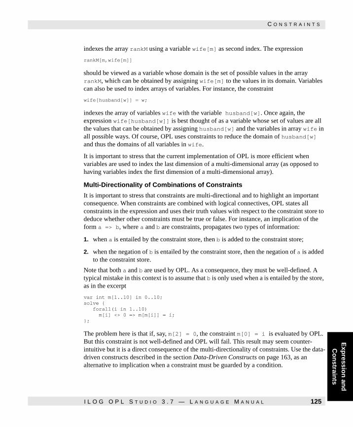
Exp
ression
and
C
on
straints
C O N S T R A I N T S
indexes the array rankM using a variable wife[m] as second index. The expression
rankM[m,wife[m]]
should be viewed as a variable whose domain is the set of possible values in the array rankM, which can be obtained by assigning wife[m] to the values in its domain. Variables can also be used to index arrays of variables. For instance, the constraint
wife[husband[w]] = w;
indexes the array of variables wife with the variable husband[w]. Once again, the expression wife[husband[w]] is best thought of as a variable whose set of values are all the values that can be obtained by assigning husband[w] and the variables in array wife in all possible ways. Of course, OPL uses constraints to reduce the domain of husband[w] and thus the domains of all variables in wife.
It is important to stress that the current implementation of OPL is more efficient when variables are used to index the last dimension of a multi-dimensional array (as opposed to having variables index the first dimension of a multi-dimensional array).
Multi-Directionality of Combinations of Constraints
It is important to stress that constraints are multi-directional and to highlight an important consequence. When constraints are combined with logical connectives, OPL states all constraints in the expression and uses their truth values with respect to the constraint store to deduce whether other constraints must be true or false. For instance, an implication of the form a => b, where a and b are constraints, propagates two types of information:
1. when a is entailed by the constraint store, then b is added to the constraint store;
2. when the negation of b is entailed by the constraint store, then the negation of a is added to the constraint store.
Note that both a and b are used by OPL. As a consequence, they must be well-defined. A typical mistake in this context is to assume that b is only used when a is entailed by the store, as in the excerpt
var int m[1..10] in 0..10; solve { forall(i in 1..10) m[i] <> 0 => m[m[i]] = i; };
The problem here is that if, say, m[2] = 0, the constraint m[0] = i is evaluated by OPL. But this constraint is not well-defined and OPL will fail. This result may seem counter-intuitive but it is a direct consequence of the multi-directionality of constraints. Use the data-driven constructs described in the section Data-Driven Constructs on page 163, as an alternative to implication when a constraint must be guarded by a condition.
I L O G O P L S T U D I O 3 . 7 — L A N G U A G E M A N U A L 125

C O N S T R A I N T S
Global Constraints
OPL also offers a variety of global constraints over discrete values. The constraint alldifferent expects an array of discrete variables/values and holds if all elements of the array are given a different value. The pruning achieved by this constraint can be specified by using the keywords onValue, onRange, onDomain. When onValue is used, OPL guarantees that, at any computation point, the variables in the array do not have the values of the already assigned variables inside their domain. When onDomain is used, OPL guarantees that, for each value in the domain of any given variable, there exist values in the domains of the remaining variables such that the constraint is satisfied. When onRange is used, the constraint enforces a pruning stronger than onValue and weaker than onDomain by reasoning only on the bounds. The constraint
alldifferent(a)
is in fact equivalent to
alldifferent(a) onValue
specifying the default of the system. The constraint circuit expects an array of integer variables, say succ, whose index set is the range 1..n. Each value in the range 1..n corresponds to a node in a graph and the value succ[i] represents the successor of node i in the graph. As a consequence, all elements in succ must range in 1..n. The constraint circuit(succ) holds if the graph so defined is a Hamiltonian circuit or, more precisely, that the sequence
(1, v1 ), (v1 , v2 ),..... (vn-1, vn), (vn, 1)
where
is a Hamiltonian circuit. We define a Hamiltonian circuit as a path through a graph that starts and ends at the same vertex and includes every other vertex exactly once. It is also known as a tour.
The constraint distribute captures a class of cardinality constraints. It expects three one-dimensional arrays card, value, and base; in addition, the arrays card and values must have the same index set. The constraint distribute(card,value,base) then holds if card[i] is the number of occurrences of value[i] in array base. If the index set of card and value is S and if the index set of base is R, then distribute(card,value,base) is equivalent to, but more efficient than
forall(i in S) card[i] = sum(j in R) (value[i] = base[j]);
126 I L O G O P L S T U D I O 3 . 7 — L A N G U A G E M A N U A L

Exp
ression
and
C
on
straints
C O N S T R A I N T S
Note that card (and, of course, base) may be arrays of variables in distribute. The pruning achieved by this constraint can be specified by the keywords basicPropagation and extendedPropagation. With keyword basicPropagation, the constraints only reasons on instantiations of values while it achieves arc-consistency when keyword extendedPropagation is used as in
distribute(s,value,s) extendedPropagation;
The default of the system is extendedPropagation. The sequence constraint clusters together several cardinality or distribute constraints to achieve a more effective pruning. More precisely, a constraint
sequence(nbMin,nbMax,width,vars,values,card)
requires that card[i] be the number of occurrences of the values[i] in array vars. In addition, it requires that each subsequence of size width in vars contains at least nbMin and at most nbMax values from values. The syntax of the constraint is as follows:
Note that the first three arguments must be integers (not variables).
The constraints atleast and atmost also capture a class of cardinality constraints. Both expect three one-dimensional arrays card, values and base. In addition, the arrays card and values must have the same index set. If the index set for the first two arrays is S, the constraint atleast(card,values,base) holds if the number of occurrences of values[i] in the array base is greater than or equal to card[i] for all i in S. Similarly, the constraint atmost(card,values,base) holds if the number of occurrences of values[i] in the array base is less than or equal to card[i] for all i in S. Note that card and base may be arrays of variables.
The constraint atleastatmost(low,up,values,base) combines the previous two constraints as it requires that the number of occurrences of values[i] in base belong to the interval low[i]..up[i]. For all three constraints, the addition of the keyword basicPropagation behind the constraint gives the user the freedom to specify a cheaper pruning level based on the instantiation of variables alone. OPL's default pruning can be obtained with the keyword extendedPropagation that achieves arc-consistency. Note that the constraint cardinality is a synonym for distribute.
Global Constraints on Aggregate Arrays
It is sometimes convenient to state a global constraint on some elements on an array. Without additional language support, it would be necessary to declare an additional array of variables
Cstr → sequence (Expr, Expr, Expr, CstrComposite, Composite, Composite)
Extended
Extended → extended
→
I L O G O P L S T U D I O 3 . 7 — L A N G U A G E M A N U A L 127

C O N S T R A I N T S
and to state equations between the new variables and the variables of interest. To remove this inconvenience, OPL provides an aggregate operator all to select elements from an array.
The statement
var int v[1..4,1..5] in 0..100; solve { alldifferent(all(i in 1..4,j in 1..5: i + j < 5) v[i,j]);};
illustrates this functionality. It selects all the elements v[i,j] such that i+j<5 and states that they must be all different. The third argument of global constraint distribute can also use an aggregate array instead of a classical array.
Predicates
Predicates in OPL let users define a constraint between a set of variables by specifying the set of compatible values for the variables. This set of tuples can be specified explicitly, by a set of records, or by an expression. It is also possible to define a constraint by specifying the set of incompatible values. The OPL implementation enforces arc consistency on predicate constraints. Arc consistency is a traditional technique from artificial intelligence that reduces the domains of variables. More precisely, a constraint c(x1 ,...., xn ) is arc-consistent with respect to the domains D1 ,...., Dn if, for each variable xi and each value vi in Di , there exist values v1 ,.....,vi-1 , vi+1 ,....,vn in D1 ,....,Di-1 , Di+1 ,...., Dn such that c(v1 ,...., vn ) holds. Enforcing arc consistency consists of removing inconsistent values from the domains until the constraint is arc-consistent with respect to the domains. The excerpt
predicate p(int i,int j,int k) in { (1,2,3) , (4,5,6), (4,5,7) };
var int x in 1..10; var int y in 1..10; var int z in 1..10;
solve { p(x,y,z); };
illustrates the use of predicates. The predicate declaration
predicate p(int i,int j,int k) in { (1,2,3) , (4,5,6), (4,5,7) g}
defines a ternary constraint whose parameters are all integers. The predicate constraint is satisfied by the tuples (1,2,3), (4,5,6), and (4,5,7). The constraint p(x,y,z) in the solve instruction enforces the predicate constraint on variables x, y, z. The resulting statement has three solutions:
{ x = 1, y = 2, z = 3 }{ x = 4, y = 5, z = 6 }{ x = 4, y = 5, z = 7 }
128 I L O G O P L S T U D I O 3 . 7 — L A N G U A G E M A N U A L

Exp
ression
and
C
on
straints
C O N S T R A I N T S
It is also interesting to understand the pruning achieved by predicate constraint. Simply stating the constraint in the above excerpt reduces the domain of x to {1,4}, of y to {2,5}, and of z to {3,6,7}. If the constraint x <> 1 is added after the predicate constraint, then variables x and y are assigned to 4 and 5 respectively and the domain of z is reduced to {6,7}. Predicate constraints can also be defined through a set of records. For instance, the previous excerpt could have been written as
struct R { int f; int s; int t; }; {R} S = { <1,2,3> , <4,5,6>, <4,5,7> }; predicate p(int i,int j,int k) in S; var int x in 1..10; var int y in 1..10; var int z in 1..10;
solve { p(x,y,z); };
The fact that predicates can be defined by sets means that the sets of possible tuples can be computed at runtime. Predicates can also be specified by defining the set of incompatible tuples. The excerpt
predicate p(int i,int j,int k) not in { (1,2,3) , (4,5,6), (4,5,7) };
var int x in 1..10; var int y in 1..10; var int z in 1..10;
solve { p(x,y,z); };
illustrates this functionality. Finally, predicates can be defined by an expression. For instance, the excerpt
predicate p(int q1,int q2,int d) return q1 <> q2 & q1 <> q2 - d & q1 <> q2 + d; var int queens[1..8] in 1..8; solve { forall(ordered i, j in 1..8) p(queens[i],queens[j],j - i); };
illustrates how to state the 8-queens problem with a predicate constraint. The predicate states that the queens q1 and q2 at distance d do not attach each other. This model achieves more pruning than the queens statement in [35] but it is, in general, less efficient. The complete syntax of predicate is shown in Partial Grammar 5.4 on page 130. Note that predicate parameters must be of integer or enumerated types.
I L O G O P L S T U D I O 3 . 7 — L A N G U A G E M A N U A L 129

C O N S T R A I N T S
Partial Grammar 5.4
Partial Grammar 5.4 The Syntax of Predicates
Scheduling Constraints
OPL also provides some specific support for scheduling applications.
Precedence Constraints
Precedence constraints between activities can be expressed easily in terms of the starting date, the ending date, and the duration of the activities. For instance, a precedence constraint between two activities a and b can be specified as b.start >= a.end However, OPL has a specific constraint for expressing precedence constraints, which is recommended since it produces better visualizations of the results. For instance, a precedence constraint between two activities a and b can be specified as a precedes b.
Resource Constraints
The most fundamental constraints in scheduling applications are of course the resource constraints that link the activities and the resources. This section describes these constraints for the various kinds of resources.
Unary Resources
Once unary resources are declared, it is possible to specify which activities require them. To specify that an activity excavation requires a resource crane in OPL, it is sufficient to write the constraint
excavation requires crane;
PredicateDecl → predicate Id (ListPredArg) PredBody
ListPredArg → PredArg { , PredArg ListPredArg }
PredArg → int Id
→ Id Id
PredBody → return Equivalence
→ in { ListPredTuples }
→ not in { ListPredTuples }
→ in Composite
→ not in Composite
ListPredTuples → PredTuple { , ListPredTuples }
PredTuples → ( ListPredValues )
ListPredValues → Integer { , LIstPredicateValues }
→ Id { , ListPredicateValues }
130 I L O G O P L S T U D I O 3 . 7 — L A N G U A G E M A N U A L
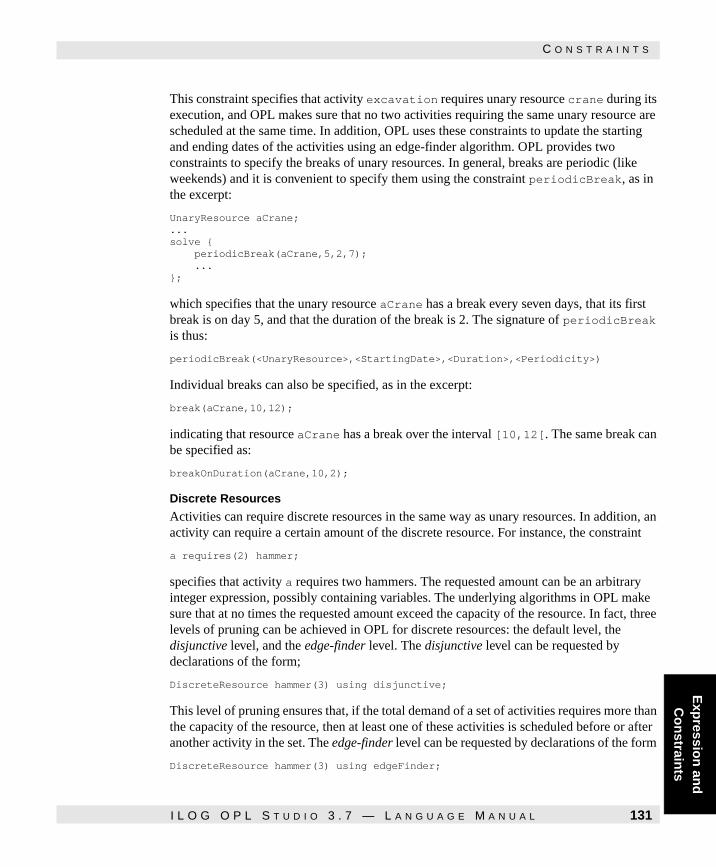
Exp
ression
and
C
on
straints
C O N S T R A I N T S
This constraint specifies that activity excavation requires unary resource crane during its execution, and OPL makes sure that no two activities requiring the same unary resource are scheduled at the same time. In addition, OPL uses these constraints to update the starting and ending dates of the activities using an edge-finder algorithm. OPL provides two constraints to specify the breaks of unary resources. In general, breaks are periodic (like weekends) and it is convenient to specify them using the constraint periodicBreak, as in the excerpt:
UnaryResource aCrane; ... solve { periodicBreak(aCrane,5,2,7); ... };
which specifies that the unary resource aCrane has a break every seven days, that its first break is on day 5, and that the duration of the break is 2. The signature of periodicBreak is thus:
periodicBreak(<UnaryResource>,<StartingDate>,<Duration>,<Periodicity>)
Individual breaks can also be specified, as in the excerpt:
break(aCrane,10,12);
indicating that resource aCrane has a break over the interval [10,12[. The same break can be specified as:
breakOnDuration(aCrane,10,2);
Discrete Resources
Activities can require discrete resources in the same way as unary resources. In addition, an activity can require a certain amount of the discrete resource. For instance, the constraint
a requires(2) hammer;
specifies that activity a requires two hammers. The requested amount can be an arbitrary integer expression, possibly containing variables. The underlying algorithms in OPL make sure that at no times the requested amount exceed the capacity of the resource. In fact, three levels of pruning can be achieved in OPL for discrete resources: the default level, the disjunctive level, and the edge-finder level. The disjunctive level can be requested by declarations of the form;
DiscreteResource hammer(3) using disjunctive;
This level of pruning ensures that, if the total demand of a set of activities requires more than the capacity of the resource, then at least one of these activities is scheduled before or after another activity in the set. The edge-finder level can be requested by declarations of the form
DiscreteResource hammer(3) using edgeFinder;
I L O G O P L S T U D I O 3 . 7 — L A N G U A G E M A N U A L 131

C O N S T R A I N T S
The edge-finder level generalizes the edge-finder algorithm of unary resources to discrete resources. It tries to deduce which activities must be scheduled first (or last) in a set whose total demand exceeds the capacity of the resource. The level of propagation appropriate depends of course on the application at hand. As mentioned previously, a constraint
a requires(2) r;
specifies that activity a requires the resource r during its execution. As a consequence, as soon as activity a terminates, its requested capacity is returned to the resource r and is available for other activities. For some applications (e.g., when the discrete resource denotes a budget), the requested capacity should not be returned to the resource: it is consumed forever. This functionality is obtained in OPL by constraints of the form
a consumes(2) r;
Note that it is also possible to use consumes for unary resources although, in general, this is not particularly useful. The capacity of a discrete resource may also vary in time, generalizing the concept of breaks in unary resources. The capacity of a discrete resource over time can be specified with constraints of the form
capacityMax(<DiscreteResource>,<Start>,<End>,<Cap>) capacityMin(<DiscreteResource>,<Start>,<End>,<Cap>)
A constraint capacityMax(d,s,e,c) specifies that the capacity of discrete resource d required by activities over the interval [s,e) is at most c, while a constraint capacityMin(d,s,e,c) specifies that the capacity of discrete resource d required by activities over the interval [s,e) is at least c. Note that this last constraint in fact constrains the scheduling of activities to make sure that they satisfy this capacity constraint.
Discrete Energy Resources
Activities can require/consume discrete energy resources in the same way as discrete resources. The underlying algorithms in OPL make sure that the total energy of the resource
Table 5.4 Reflective Methods on Discrete Energy Resources.
Method Type Semantics
getEnergyMax(int t) int the maximum energy that can be used at time t
getEnergyMin(int t) int the minimum energy that must be used at time t
getEnergyMaxMax(int m,int M) int the maximum energy over [m,M)
getEnergyMaxMin(int m,int M) int the maximum of the minimum energy over [m,M)
getEnergyMinMax(int m,int M) int the minimum of the maximum energy over [m,M)
getEnergyMinMin(int m,int M) int the minimum energy over [m,M)
132 I L O G O P L S T U D I O 3 . 7 — L A N G U A G E M A N U A L

Exp
ression
and
C
on
straints
C O N S T R A I N T S
at the various time intervals is not exceeded. The energy of a discrete energy resource over time can be specified with methods whose signatures are
setEnergyMin(<Start>,<End>,<Energy>) setEnergyMax(<Start>,<End>,<Energy>)
For instance, if d is a discrete energy resource, then the method
d.setEnergyMin(1,5,2)
specifies that the energy of d over time interval [1,5) is no less than 2, while the method
d.setEnergyMax(1,5,5)
specifies that the energy of d over time interval [1,5) is no more than 5. OPL also supports a number of reflective methods on discrete energy resources that are depicted in Table 5.4 on page 132. These methods give access to the possible energy of the resource at various times or time intervals. For instance, the method getEnergyMaxMin(int m,int M) considers the minimal energies that can be used at a time t in the interval [m,M) and returns the maximal value.
Reservoirs
Reservoirs support the same constraints as discrete resources. In addition, they also support constraints allowing activities to provide and produce some units of the resources. Assuming that plumbing and tank are declared as reservoirs,
a requires(2) plumbing;
specifies that activity a requires two units of plumbing during its execution. Activities can also consume the reservoir, as in
a consumes(2) tank;
which specifies that activity a consumes 2 units of reservoir tank (and does not return these two units at the end of its execution). Constraint
b provides(2) plumbing;
specifies that activity b provides two units of plumbing during its execution, while constraint
b produces(2) oil;
specifies that activity b produces two units of oil from its ending date to the horizon. Of course, providing and producing are the counterparts to requiring and consuming.
State Resources
Activities may require that a state resource be in a given state during their execution. For instance, the oven must be warm for some pastries and hot for some others. The constraint
a requiresState(warm) oven;
I L O G O P L S T U D I O 3 . 7 — L A N G U A G E M A N U A L 133
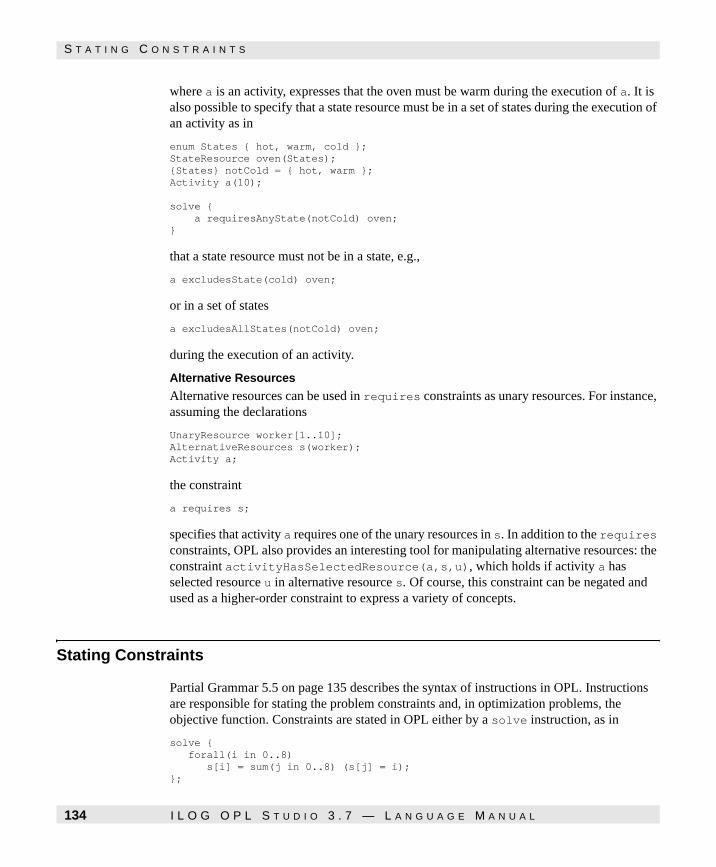
S T A T I N G C O N S T R A I N T S
where a is an activity, expresses that the oven must be warm during the execution of a. It is also possible to specify that a state resource must be in a set of states during the execution of an activity as in
enum States { hot, warm, cold }; StateResource oven(States); {States} notCold = { hot, warm }; Activity a(10);
solve { a requiresAnyState(notCold) oven; }
that a state resource must not be in a state, e.g.,
a excludesState(cold) oven;
or in a set of states
a excludesAllStates(notCold) oven;
during the execution of an activity.
Alternative Resources
Alternative resources can be used in requires constraints as unary resources. For instance, assuming the declarations
UnaryResource worker[1..10]; AlternativeResources s(worker); Activity a;
the constraint
a requires s;
specifies that activity a requires one of the unary resources in s. In addition to the requires constraints, OPL also provides an interesting tool for manipulating alternative resources: the constraint activityHasSelectedResource(a,s,u), which holds if activity a has selected resource u in alternative resource s. Of course, this constraint can be negated and used as a higher-order constraint to express a variety of concepts.
Stating Constraints
Partial Grammar 5.5 on page 135 describes the syntax of instructions in OPL. Instructions are responsible for stating the problem constraints and, in optimization problems, the objective function. Constraints are stated in OPL either by a solve instruction, as in
solve { forall(i in 0..8) s[i] = sum(j in 0..8) (s[j] = i); };
134 I L O G O P L S T U D I O 3 . 7 — L A N G U A G E M A N U A L

Exp
ression
and
C
on
straints
S T A T I N G C O N S T R A I N T S
or by an optimization instruction, as in
minimize sum(p in Products) (insideCost[p]*inside[p] + outsideCost[p]*outside[p]) subject to { forall(r in Resources) sum(p in Products) consumption[p,r] * inside[p] <= capacity[r]; forall(p in Products) inside[p] + outside[p] >= demand[p]; };
Note that the optimization instructions require an objective function of type integer or float.
Partial Grammar 5.5
Partial Grammar 5.5 The Syntax of Instructions
Linear Relaxation
The keyword with linear relaxation may be added after the solve, minimize, or maximize instructions. Its effect is to add the linear relaxation of any integer constraint to the constraint store. In other words, the constraint store receives the relaxation of an integer constraint c whenever c becomes a float constraint when all its integer variables are considered of type float. This feature is discussed again in Chapter 14, Constraint Programming.
Universal Quantifiers
OPL provides a universal quantifier to declare a collection of closely related constraints. For instance, the excerpt
forall(i in 0..8) s[i] = sum(j in 0..8) (s[j] = i);
states the constraints
s[0] = sum(j in 0..8) (s[j] = 0); .... s[8] = sum(j in 0..8) (s[j] = 8);
Instr → solve Relax Cstr;
→ minimize Relax Expr subject to Cstr;
→ maximize Relax Expr subject to Cstr;
I L O G O P L S T U D I O 3 . 7 — L A N G U A G E M A N U A L 135

S T A T I N G C O N S T R A I N T S
It is possible to use nested forall statements, as in
forall(i in 1..8) forall(j in [i+1..8]) queen[i] <> queen[j]
forall statements can also contain a block, e.g.
forall(i in 1..8) forall(j in [i+1..8]) { queen[i] <> queen[j]; queen[i] - i <> queen[j] - j; queen[i] + i <> queen[j] + j; };
Of course, the above statement can be written more concisely as
forall(ordered i,j in 1..8) { queen[i] <> queen[j]; queen[i] - i <> queen[j] - j; queen[i] + i <> queen[j] + j; };
OPL offers a rich set of formal parameters, as described in more detail in Chapter 6, Formal Parameters.
Conditional Statements
if-then-else statements make it possible to state constraints conditionally, as in
forall(<f,g,d> in Distances) if d > 1 then abs(freq[f] - freq[g]) >= d else freq[f] <> freq[g] endif;
Conditions in if-then-else statements must be ground, i.e., they must not contain variables (except, possibly, in reflective functions). Implications of constraints can be used instead when conditions contain variables.
Naming Constraints
Constraints can also be given a name, as in
constraint capacityCons[Resources]; constraint demandCons[Products];
minimize sum(p in Products) (insideCost[p]*inside[p] + outsideCost[p]*outside[p]) subject to { forall(r in Resources) capacityCons[r]: sum(p in Products) consumption[p,r] * inside[p] <= capacity[r]; forall(p in Products) demandCons[p]: inside[p] + outside[p] >= demand[p]; };
This statement is equivalent to the statement
minimize sum(p in Products) (insideCost[p]*inside[p] + outsideCost[p]*outside[p]) subject to { forall(r in Resources) sum(p in Products) consumption[p,r] * inside[i] <= capacity[r]; forall(p in Products)
136 I L O G O P L S T U D I O 3 . 7 — L A N G U A G E M A N U A L

Exp
ression
and
C
on
straints
S T A T I N G C O N S T R A I N T S
inside[p] + outside[p] >= demand[p]; };
shown earlier in this section. The only difference is that the constraints have been given a name that can be used to display the data. This functionality is often useful to find which constraints are tight in applications as well to find the values of dual variables in linear programs.
Constraint Expressions
OPL makes it possible to retrieve a variety of information about constraints. If c is a constraint, c.dual denotes the value of the associated dual variable, c.slack its slack, c.lhs the value of its left-hand side, and c.rhs the value of its right-hand side. For dual variables, OPL takes the convention that constraints of the form l <= r are rewritten into l - r <= 0 and constraints of the form l >= r into l - r >= 0. If c is a constraint of the form l <= m <= u, c.left denotes the constraint l <= m and c.right denotes the constraint m <= u. These accessors also apply to other operators and more sophisticated sequences. They make it possible to retrieve individual constraints and their associated information.
Basis Status
When a linear program is solved, OPL gives access to the basis information associated with the optimal solution. Each variable and each constraint has an associated attribute called status. This attribute is of type BasisStatus, a predefined enumerated type stated as:
enum BasisStatus {atLower, atUpper, inBasis, noBasis, freeSuper};
The semantics of the status attribute in the context of a variable is defined as follows:
◆ atLower The variable is at its lower bound
◆ atUpper The variable is at its upper bound
◆ inBasis The variable is basic
◆ noBasis No basis information is associated with this variable
◆ freeSuper The variable is free and non-basic.
I L O G O P L S T U D I O 3 . 7 — L A N G U A G E M A N U A L 137

S T A T I N G C O N S T R A I N T S
The semantics of the status attribute in the context of a constraint is defined as follows:
◆ noBasis No basis information was defined for this constraint
◆ atLower The associated slack/surplus/artificial variable is non-basic and at value 0.0
◆ inBasis The associated slack/surplus/artificial variable is basic.
The status attribute can be manipulated by any OPL statement and can be stored in other user declared objects of type BasisStatus. For instance, consider Statement 5.1. It solves the production model and uses the status field of the variable to only display the variables that are in the basis. The output is shown in Statement 5.2 on page 139.
Statement 5.1
Statement 5.1 Using The Status Field.
enum Products ...; enum Resources ...; float+ comsumption[Products,Resources] = ...; float+ capacity[Resources] = ...; float+ demand[Products] = ...; float+ insideCost[Products] = ...; float+ outsideCost[Products] = ...;
var float+ inside[Products]; var float+ outside[Products]; constraint capCstr[Resources];
minimize sum(p in Products) (insideCost[p]*inside[p] + outsideCost[p]*outside[p]) subject to { forall( r in Resources) capCstr[r]: sum(p in Products) consumption[p,r] * inside[p] <= capacity[r];
forall( p in Products) inside[p] + outside[p] >= demand[p]; };
BasisStatus status[p in Products] = inside[p].status; display(p in Products) <inside[p],inside[p].status>; display(p in Products) <outside[p],outside[p].status>; display(p in Products : status[p] = inBasis) inside[p]; display(p in Products : outside[p].status = inBasis) outside[p]; display(r in Resources) capCstr[r].status;
138 I L O G O P L S T U D I O 3 . 7 — L A N G U A G E M A N U A L

Exp
ression
and
C
on
straints
S T A T I N G C O N S T R A I N T S
Statement 5.2
Statement 5.2 Output From The Production Model.
<inside[kluski],inside[kluski].status> = <40.0000,inBasis> <inside[capellini],inside[capellini].status> = <0.0000,atLower> <inside[fettucine],inside[fettucine].status> = <0.0000,atLower>
<outside[kluski],outside[kluski].status> = <60.0000,inBasis> <outside[capellini],outside[capellini].status> = <200.0000,inBasis> <outside[fettucine],outside[fettucine].status> = <300.0000,inBasis>
inside[kluski] = 40.0000
outside[kluski] = 60.0000 outside[capellini] = 200.0000 outside[fettucine] = 300.0000
capCstr[flour].status = atLower capCstr[eggs].status = inBasis
I L O G O P L S T U D I O 3 . 7 — L A N G U A G E M A N U A L 139

S T A T I N G C O N S T R A I N T S
140 I L O G O P L S T U D I O 3 . 7 — L A N G U A G E M A N U A L

C H A P T E R
Fo
rmal P
arameters
6
Formal Parameters
Formal parameters play a fundamental role in OPL: they are used in aggregate operators, queries, and forall statements. This chapter reviews them in more detail.
You can find information on the following topics:
◆ Basic Formal Parameters on page 142 describes the basic formal parameters.
◆ Tuples of Parameters on page 144 shows how to use tuples of formal parameters.
◆ Filtering in Tuples of Parameters on page 145 studies how tuples of parameters can be used for filtering.
◆ Modeling Issues on page 145 discusses a number of modeling issues that arise when using parameters.
◆ Partial Grammar 6.1 on page 142 depicts the syntax of parameters in OPL.
I L O G O P L S T U D I O 3 . 7 — L A N G U A G E M A N U A L 141

B A S I C F O R M A L P A R A M E T E R S
Basic Formal Parameters
The simplest formal parameter has the form
p in S
where p is the formal parameter and S is the set from which p takes its values. The set S can be an integer range, as in
int s = sum(i in 1..n) i*i;
an enumerated type, as in
enum Products ...; float+ cost[Products] = ...; float+ maxCost = max(p in Products) cost[p];
or a finite set, as in
enum Cities ...; struct Connection { Cities orig; Cities dest; }; {Connection} connections = ...; float+ cost[connections] = ...; float+ maxCost = max(r in connections) cost[r];
It is sometimes desirable to restrict the range of the formal parameters using conditions. The formal parameter then takes the form
p in S : condition
and assigns to p all elements of S satisfying the condition.Partial Grammar 6.1
Partial Grammar 6.1 The Parameters Syntax
For instance, the excerpt
forall(i in 1..8) forall(j in 1..8 : i < j) queen[i] <> queen[j];
ListParameter → Parameter
→ Parameter, ListParameter
→ Parameter & ListParameter
Parameter → Parameter
→ Object+ in Bounds→ Ordered Object+ in Bounds→ Object+ in Bounds : Relation→ Ordered Object+ in Bounds : Relation
Object → Id | <Id+>
Bounds → Composite | Range
142 I L O G O P L S T U D I O 3 . 7 — L A N G U A G E M A N U A L

B A S I C F O R M A L P A R A M E T E R S
Fo
rmal P
arameters
the constraint queen[i] <> queen[j] for all 1 ≤ i < j ≤ 8. Several parameters can often be combined together to produce more compact statements. For instance, the declaration
int s = sum(i,j in 1..n) i*j;
is equivalent to
int s = sum(i in 1..n) sum(j in 1..n) i*j;
which is less readable. The declaration
int s = sum(i in 1..n & j in 1..m) i*j;
where the ranges of i and j are different, is equivalent to
int s = sum(i in 1..n, j in 1..m) i*j;
where a comma has been substituted for &, and to
int s = sum(i in 1..n) sum(j in 1..m) i*j;
These parameters can, of course, be subject to conditions. The excerpt
forall(i,j in 1..8 : i < j) queen[i] <> queen[j];
is equivalent to
forall(i in 1..8 & j in 1..8 : i<j) queen[i] <> queen[j];
and to the excerpt shown earlier in this chapter. The even more compact form
forall(ordered i,j in 1..8) queen[i] <> queen[j];
is equivalent to the excerpts just shown and illustrates a functionality, i.e., ordered, often useful in practical applications. Indeed, in many applications one is interested, given a set S, to state constraints or conditions over all pairs (i, j) of elements of S satisfying i < j in the ordering associated with S. Note that S may be a range, an enumerated type, or any finite set, since these are all ordered. For instance, the excerpt
enum Tasks ...; enum Resources ...; {Tasks} res[Resources] = ...; ... int duration[Tasks] = ...; var int start[Tasks] in 0..10000; solve { forall(r in Resources & ordered t1,t2 in res[r]) start[t1] >= start[t2] + duration[t2] \/ start[t2] >= start[t1] + duration[t1]; ... };
illustrates this functionality on an enumerated type Task. The quantifier considers all pairs (t1,t2) in the set of tasks res[r] such that t1 < t2.
I L O G O P L S T U D I O 3 . 7 — L A N G U A G E M A N U A L 143

T U P L E S O F P A R A M E T E R S
Tuples of Parameters
OPL also allows tuples of formal parameters to appear in aggregate operators, forall statements, and queries. Consider the excerpt
enum Tasks ...; struct Precedence { Tasks before: Tasks after; }; {Precedence} Prec = ...; int duration[Tasks] = ...; var int start[Tasks] in 0..maxTime; solve { forall(p in Prec) start[p.after] >= start[p.before] + duration[p.before]; };
which states precedence constraints between tasks. The constraint declaration requires explicit accesses to the fields of the record to state the constraints. In addition, the field before is accessed twice. A more elegant way to state the same constraint is to use a tuple of formal parameters, as in
forall(<b,a> in Prec) start[a] >= start[b] + duration[b]
precluding the need to access the record fields explicitly. The tuple <b,a> in the forall quantifier contains two parameters that are given the values of the fields of each record in Prec successively. More generally, an expression
p in S
where S is a set of records containing n fields, can be replaced by a formal parameter expression
<p1,...,pn> in S
that contains n formal parameters. Each time a record r is selected from S, its fields are assigned to the corresponding formal parameters. This functionality is often useful in producing more readable models. (Note that this functionality is not (yet) available for membership constraints.)
144 I L O G O P L S T U D I O 3 . 7 — L A N G U A G E M A N U A L

F I L T E R I N G I N T U P L E S O F P A R A M E T E R S
Fo
rmal P
arameters
Filtering in Tuples of Parameters
OPL also enables simple equality constraints to be factorized inside the tuples, which is important in obtaining more readable and efficient models. Consider, for instance, a transportation problem where products must be shipped from a set of cities to another set of cities. The model may include a constraint specifying that the total shipments for all products transported along a connection may not exceed a specified limit. This can be expressed by a constraint
forall(c in connections) sum(<p,co> in routes : c = co) trans[<p,c>] <= limit;
This constraint states that the total products shipped along each connection c is not greater than limit. This statement is particularly inefficient: OPL must scan the entire set routes to select the tuples involving each connection. The constraint would be stated more efficiently as follows
forall(c in connections) sum(<p,c> in routes) trans[<p,c>] <= limit;
In this last constraint, the tuple <p,c> contains one new parameter p and uses the previously defined parameter c. Since the value of c is known, OPL uses it to index the set routes, avoiding a complete scanning of the set routes.
Modeling Issues
It is useful at this point to discuss some modeling issues involving sparsity, tuples of parameters, and filtering. An application can often be described by various models that may exhibit fundamentally different performance in terms of memory and computing time. This is particularly important for large-scale linear models. Consider again the transportation problem in which the shipments of products between each pair of cities may not exceed a given limit. Statement 6.1 on page 146 shows a simple model for this problem, which implicitly assumes that all cities are connected and that all products may be shipped between two cities. It is thus not appropriate for large-scale problems where only a fraction of the cities are connected. A small data set can easily illustrate the issue: Consider the set of cities
{Amsterdam,Antwerpen,Bergen,Bonn,Brussels,Cassis,London,Madrid,Milan,Paris}
and the set of products {Godiva,Leonidas,Neuhaus}. There are three hundred ways of shipping a product from a city to another. However, only a small fraction of these may be explored in the application and Figure 6.1 displays a possible subset.
I L O G O P L S T U D I O 3 . 7 — L A N G U A G E M A N U A L 145

M O D E L I N G I S S U E S
Using Statement 6.1 would induce a substantial loss in (memory and time) efficiency. The rest of this section explores how to exploit this sparsity.
Statement 6.1
Statement 6.1 A Simple Transportation Model (transp1.mod).
Figure 6.1 A Sparse Data Set for a Transportation Problem
enum Cities ...; enum Products ...; float+ limit = ...; float+ supply[Products,Cities] = ...; float+ demand[Products,Cities] = ...; assert forall(p in Products) sum(o in Cities) supply[p,o] = sum(d in Cities) demand[p,d];float+ cost[Products,Cities,Cities] = ...;
var float+ trans[Products,Cities,Cities]; minimize sum(p in Products & o,d in Cities) cost[p,o,d] * trans[p,o,d]subject to { forall(p in Products & o in Cities) sum(d in Cities) trans[p,o,d] = supply[p,o]; forall(p in Products & d in Cities) sum(o in Cities) trans[p,o,d] = demand[p,d]; forall(o, d in Cities) sum(p in Products) trans[p,o,d] <= limit; };
<Godiva,Brussels,Paris> <Godiva,Brussels,Bonn> <Godiva,Amsterdam,London>
<Godiva,Amsterdam,Milan> <Godiva,Antwerpen,Madrid> <Godiva,Antwerpen,Bergen>
<Neuhaus,Brussels,Milan> <Neuhaus,Brussels,Bergen> <Neuhaus,Amsterdam,Madrid>
<Neuhaus,Amsterdam,Cassis> <Neuhaus,Antwerpen,Paris> <Neuhaus,Antwerpen,Bonn>
<Leonidas,Brussels,Bonn> <Leonidas,Brussels,Milan> <Leonidas,Amsterdam,Paris>
<Leonidas,Amsterdam,Cassis> <Leonidas,Antwerpen,London> <Leonidas,Antwerpen,Bergen>
146 I L O G O P L S T U D I O 3 . 7 — L A N G U A G E M A N U A L

M O D E L I N G I S S U E S
Fo
rmal P
arameters
A First Attempt
A first attempt at exploiting the sparsity available in a large-scale transportation problem consists of representing the data as a set routes of records of type
struct Route { Prod p; Cities o; Cities d; g}
The array cost and trans can then be indexed with this set. A model based on this idea appears in Statement 6.2.
Statement 6.2
Statement 6.2 A Sparse Transportation Model: First Attempt (transp2.mod).
The data for the supplies and demands are also represented in a sparse way by projecting the set routes to obtain their index sets. In addition to that, the model also precomputes, in a generic way, the cities orig[p] that can ship product p and the cities dest[p] that can receive product p. Most of the resulting model is elegant and efficient.
enum Cities ...; enum Products ...; float+ limit = ...;
struct Route { Products p; Cities o; Cities d; }; {Route} routes = ...; struct Supply { Products p; Cities o; }; {Supply} Supplies = { <p,o> | <p,o,d> in routes }; float+ supply[Supplies] = ...; struct Demand { Products p; Cities d; }; {Demand} Demands = { <p,d> | <p,o,d> in routes }; float+ demand[Demands] = ...; float+ cost[routes] = ...;
{Cities} orig[p in Products] = { o | <p,o,d> in routes }; {Cities} dest[p in Products] = { d | <p,o,d> in routes }; {Connection} CP[p in Products] = { c | <p,c> in Routes }; assert forall(p in Products) sum(o in orig[p]) supply[<p,o>] = sum(d in dest[p]) demand[<p,d>]; var float+ trans[routes];
minimize sum(l in routes) cost[l] * trans[l] subject to { forall(p in Products & o in orig[p]) sum(<o,d> in CP[p]) trans[<p,o,d>] = supply[<p,o>]; forall(p in Products & d in dest[p]) sum(<o,d> in CP[p]) trans[<p,o,d>] = demand[<p,d>]; forall(o,d in Cities) sum(<p,o,d> in routes) trans[<p,o,d>] <= limit; };
I L O G O P L S T U D I O 3 . 7 — L A N G U A G E M A N U A L 147

M O D E L I N G I S S U E S
Unfortunately, the constraint
forall(o in Orig & d in Dest) sum(<p,o,d> in routes) trans[<p,o,d>] <= limit;
is not particularly efficient because it does not exploit the structure of the application. Indeed, the forall statement iterates not over actual connections but rather over all pairs of cities. In addition, the aggregate operator
sum(<p,o,d> in routes) trans[<p,o,d>] <= limit;
cannot exploit the “connection” structure to obtain all products of a connection, since o and d are separate entities.
A Better Model
The application can be modeled more effectively by closely reflecting the structure of the application. Statement 6.3 on page 149 gives a statement illustrating this principle. The main novelty is the explicit representation of connections and the fact that a route is now simply the association of a connection and a product. Connections are also computed automatically from routes. The rest of the model is generally similar but reflects the new data organization. The most interesting change is the capacity constraint, which becomes
forall(c in connections) sum(<c,p> in routes) trans[<c,p>] <= limit;
This constraint is much more efficient than in the previous model. First, it iterates over the routes, not over all pairs of cities. Second, the aggregate operator sum uses parameter c to index the set routes, retrieving the relevant products effectively.
148 I L O G O P L S T U D I O 3 . 7 — L A N G U A G E M A N U A L

M O D E L I N G I S S U E S
Fo
rmal P
arameters
Statement 6.3
Statement 6.3 A Sparse Transportation Model: Second Attempt (transp3.mod).
enum Cities ...; enum Products ...;
struct Connection { Cities o; Cities d; }; struct Route { Connection e; Products p; }; struct Supplier { Products p; Cities o; }; struct Customer { Products p; Cities d; };
{Route} Routes = ...; {Connection} Connections = { c | <c,p> in Routes }; {Supplier} Suppliers = { <p,c.o> | <c,p> in Routes }; float+ supply[Suppliers] = ...; {Customer} Customers = { <p,c.d> | <c,p> in Routes }; float+ demand[Customers] = ...; float+ lim = ...; float+ cost[Routes] = ...; {Cities} orig[p in Products] = { c.o | <c,p> in Routes }; {Cities} dest[p in Products] = { c.d | <c,p> in Routes }; {Connection} CP[p in Products] = { c | <p,c> in Routes };
assert forall(p in Products) sum(o in orig[p]) supply[<p,o>] = sum(d in dest[p]) demand[<p,d>];
var float+ trans[Routes];
minimize sum(r in Routes) cost[r] * trans[r] subject to { forall(p in Products & o in orig[p]) sum(<o,d> in CP[p]) trans[< <o,d>,p>] = supply[<p,o>]; forall(p in Products & d in dest[p]) sum(<o,d> in CP[p]) trans[< <o,d>,p>] = demand[<p,d>]; forall(c in Connections) sum(<c,p> in Routes) trans[<c,p>] <= lim; };
I L O G O P L S T U D I O 3 . 7 — L A N G U A G E M A N U A L 149

M O D E L I N G I S S U E S
150 I L O G O P L S T U D I O 3 . 7 — L A N G U A G E M A N U A L

C H A P T E R
Search
7
Search
One of the main novelties of OPL is its ability to specify search procedures. This support is fundamental for hard combinatorial optimization problems, where search is necessary. Indeed, constraint-solving algorithms are typically incomplete and cannot solve optimization problems alone, except in some specific classes of applications such as linear programming. The constraint-solving algorithms usually solve relaxations of the problem and are complemented by search procedures. Traditionally, modeling languages and most mathematical programming packages hide these search procedures from users, who can control them only through a set of parameters. OPL also has a number of default search procedures. In addition, it offers the ability to specify search procedures tailored to the application at hand. This functionality, at the core of traditional constraint programming languages, can lead to significant improvements in performance by incorporating special-purpose heuristics in the model. It is important to emphasize that the search procedure is optional and may be partial (e.g., not all variables are given a value). OPL simply applies its default search procedures once the user-defined search has been executed. The syntax of search procedures is given in Partial Grammar 7.1 on page 193 and this chapter reviews the various constructs available.
I L O G O P L S T U D I O 3 . 7 — L A N G U A G E M A N U A L 151

T H E T R Y I N S T R U C T I O N
The Try Instruction
Many applications use search algorithms that generate values for the variables. OPL has a number of constructs to express these procedures. Its most basic control structure is the try instruction, for example
try x = 1 | x = 2 endtry;
The try instruction is nondeterministic and specifies a number of alternatives to be explored. The instruction in the example tells OPL to assign x to either 1 or 2; it succeeds if one of these alternatives is consistent with the constraint store and it fails otherwise. Operationally, OPL tries the first alternative and adds the constraint x = 1 to the constraint store. When the constraint is added to the store, OPL either detects a failure (i.e., the constraint is not consistent with the store), in which case the next alternative is selected, or succeeds, in which case OPL moves on to the next instructions, i.e., the instructions following the try if any. The execution of these subsequent instructions may fail, in which case the other alternative to the try (i.e. x = 2) is considered. For instance, the model
var int x in 1..5; solve { x <> 1; }; search { try x = 1 | x = 2 | x = 3 | x = 4 | x = 5 endtry; };
adds the constraint x = 1, which produces a failure. It then adds the constraint x = 2, which succeeds and produces the solution x = 2. If another solution is requested, OPL backtracks, selects the next alternative x = 3, and produces the solution x = 3. The other solutions are produced in a similar fashion.
It is interesting to study what happens when several try instructions are used in sequence. Consider the model
var int x in 0..1; var int y in 0..1; solve { x + y <=1; }; search { try x = 1 | x = 0 endtry; try y = 1 | y = 0 endtry; };
Here OPL considers the first try instruction and adds the constraint x = 1. It then moves to the next instruction and adds the constraint y = 1, which results in a failure. OPL then backtracks to the second alternative and produces the solution
152 I L O G O P L S T U D I O 3 . 7 — L A N G U A G E M A N U A L

Search
T H E T R Y A L L I N S T R U C T I O N
Solution [1] x = 1 y = 0
If additional solutions are requested, OPL backtracks to the second try instruction. Since no alternatives remain, it then backtracks to the first try instruction and restores the constraint store to the exact same state as when the try instruction was first executed. The constraint store at that point only contains the constraint x + y <= 1. OPL then selects the second alternative x = 0, moves to the next instruction, selects the first alternative, and produces the solution
Solution [2] x = 0 y = 1
The tryall Instruction
The try instruction is convenient when the set of alternatives is small and does not depend on the input data. The tryall instruction can be viewed as a compact and dynamic representation of the try instruction. For instance, the instruction
tryall(i in 1..5) x = i;
is equivalent to the instruction
try x = 1 | x = 2 | x = 3 | x = 4 | x = 5 endtry;
It first assigns 1 to parameter i and adds the constraint x = i to the constraint store. If it succeeds, the execution proceeds to the next instruction. Otherwise, the instruction assigns the value 2 to i and adds the constraint x = i again. This time, however, the constraint corresponds to x = 2. The tryall instruction can also specify the order in which the alternatives should be tried. For instance, the instruction
tryall(i in 1..5 ordered by increasing i) x = i;
tries the values for i in the order 1,2,.....,5, while the instruction
tryall(i in 1..5 ordered by decreasing i) x = i;
tries the values in the order 5,4,.....,1. Note that the ordering can be specified by an arbitrary expression that may contain some reflective functions. Finally, it is useful to mention that the tryall instruction may include a condition, as in
tryall(i in 1..10 : i mod 3 = 0) x = i;
I L O G O P L S T U D I O 3 . 7 — L A N G U A G E M A N U A L 153

Q U A N T I F I E R S
which is equivalent to
try x = 3 | x = 6 | x = 9 endtry;
The condition can be used to filter out some undesired elements.
Quantifiers
The other fundamental choice instruction is a universal quantifier (or iterative statement) that is similar in spirit to the universal quantifier of constraint specifications. However, the formal parameters allowed in the forall statement of search procedures (as well as in other constructs such as tryall and select) are a subset of those available for constraints. This restriction is motivated by the need to define dynamic orderings, which are often important in practice.
To illustrate the forall instruction, consider the following statement, which solves the four-queens problem and specifies a search procedure:
var int queen[1..4] in 1..4; solve { forall(ordered i, j in 1..4) { queen[i] <> queen[j]; queen[i] + i <> queen[j] + j; queen[i] - i <> queen[j] - j; } }; search { forall(i in 1..4) tryall(v in 1..4) queen[i] = v; };
The search procedure specifies considering each queen in turn (i.e., queen[1],...,queen[4]) and assigning them the values 1..4 nondeterministically. This search procedure is in fact equivalent to
search { try queen[1] = 1 | queen[1] = 2 | queen[1] = 3 | queen[1] = 4 endtry; try queen[2] = 1 | queen[2] = 2 | queen[2] = 3 | queen[2] = 4 endtry; try queen[3] = 1 | queen[3] = 2 | queen[3] = 3 | queen[3] = 4 endtry; try queen[4] = 1 | queen[4] = 2 | queen[4] = 3 | queen[4] = 4 endtry; };
When the model is executed, the search procedure assigns the value 1 to queen[1]. It then tries assigning a value to queen[2] but all values fail. The search procedure then backtracks and assigns the value 2 to queen[1]. It then tries the values 1..4 for queen[2]. Values 1..3 lead to failures but value 4 succeeds and assigns values 1 and 3 to queen[3] and queen[4], respectively. The last two tryall instructions succeed for their first and third alternatives.
154 I L O G O P L S T U D I O 3 . 7 — L A N G U A G E M A N U A L
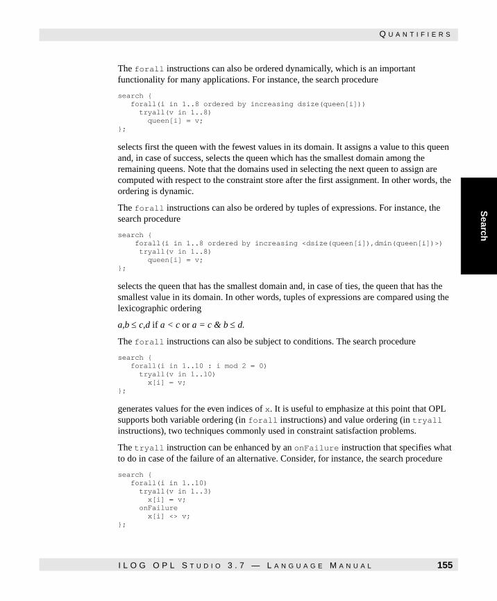
Search
Q U A N T I F I E R S
The forall instructions can also be ordered dynamically, which is an important functionality for many applications. For instance, the search procedure
search { forall(i in 1..8 ordered by increasing dsize(queen[i])) tryall(v in 1..8) queen[i] = v; };
selects first the queen with the fewest values in its domain. It assigns a value to this queen and, in case of success, selects the queen which has the smallest domain among the remaining queens. Note that the domains used in selecting the next queen to assign are computed with respect to the constraint store after the first assignment. In other words, the ordering is dynamic.
The forall instructions can also be ordered by tuples of expressions. For instance, the search procedure
search { forall(i in 1..8 ordered by increasing <dsize(queen[i]),dmin(queen[i])>) tryall(v in 1..8) queen[i] = v; };
selects the queen that has the smallest domain and, in case of ties, the queen that has the smallest value in its domain. In other words, tuples of expressions are compared using the lexicographic ordering
a,b ≤ c,d if a < c or a = c & b ≤ d.
The forall instructions can also be subject to conditions. The search procedure
search { forall(i in 1..10 : i mod 2 = 0) tryall(v in 1..10) x[i] = v; };
generates values for the even indices of x. It is useful to emphasize at this point that OPL supports both variable ordering (in forall instructions) and value ordering (in tryall instructions), two techniques commonly used in constraint satisfaction problems.
The tryall instruction can be enhanced by an onFailure instruction that specifies what to do in case of the failure of an alternative. Consider, for instance, the search procedure
search { forall(i in 1..10) tryall(v in 1..3) x[i] = v; onFailure x[i] <> v; };
I L O G O P L S T U D I O 3 . 7 — L A N G U A G E M A N U A L 155

S E Q U E N C I N G C H O I C E S
The key idea behind this search procedure is to add the constraint x[i] <> v each time an alternative x[i] = v fails. In other words, this search procedure is equivalent to
search { forall(i in 1..10) try x[i] = 1 | { x[i] <> 1; try x[i] = 2 | { x[i] <> 2; x[i] = 3; } endtry } endtry };
Of course, the onFailure can be followed by an arbitrary search procedure, not just a constraint.
Sequencing Choices
As should be clear, search procedures in OPL are sequences of instructions. The search procedure
search { try x = 1 | x = 2 endtry; try y = 1 | y = 2 endtry; };
executes the first try instruction and, in case of success, proceeds to the second try instruction. Of course, the sequences may contain arbitrary choice instructions, including forall and tryall instructions. For instance, the search procedure
search { forall(i in 1..3) tryall(v in 1..3) x[i] = v; forall(j in 1..3) tryall(w in 1..3) y[j] = w; };
specifies a sequence of two forall instructions.
This search procedure could be written, by changing only the names of the formal parameters, as
search { forall(i in 1..3) tryall(v in 1..3) x[i] = v; forall(i in 1..3) tryall(v in 1..3) y[i] = v; };
since the scope of the parameters in forall and tryall statements is the body of their instructions. Note that the above search procedure is fundamentally different from
search { forall(i in 1..3) {
156 I L O G O P L S T U D I O 3 . 7 — L A N G U A G E M A N U A L

Search
C O N D I T I O N A L C H O I C E S
tryall(v in 1..3) x[i] = v; tryall(v in 1..3) y[i] = v; }; };
Indeed, the former search procedure is equivalent to
search { try x[1] = 1 | x[1] = 2 | x[1] = 3 endtry; try x[2] = 1 | x[2] = 2 | x[2] = 3 endtry; try x[3] = 1 | x[3] = 2 | x[3] = 3 endtry; try y[1] = 1 | y[1] = 2 | y[1] = 3 endtry; try y[2] = 1 | y[2] = 2 | y[2] = 3 endtry; try y[3] = 1 | y[3] = 2 | y[3] = 3 endtry; };
while the latter is equivalent to
search { try x[1] = 1 | x[1] = 2 | x[1] = 3 endtry; try y[1] = 1 | y[1] = 2 | y[1] = 3 endtry; try x[2] = 1 | x[2] = 2 | x[2] = 3 endtry; try y[2] = 1 | y[2] = 2 | y[2] = 3 endtry; try x[3] = 1 | x[3] = 2 | x[3] = 3 endtry; try y[3] = 1 | y[3] = 2 | y[3] = 3 endtry; };
Conditional Choices
Conditionals can also be used in OPL to make different choices according to the truth value of a condition. For instance, the search procedure
search { forall(i in 1..10) if i mod 2 = 0 then tryall(v in 1..10 ordered by increasing i) x[i] = v else tryall(v in 1..10 ordered by decreasing i) x[i] = v endif; }
uses a different value ordering for the variables with even and odd indices. Note that the condition in the conditional statement must not contain variables except, of course, in reflective functions.
I L O G O P L S T U D I O 3 . 7 — L A N G U A G E M A N U A L 157

T H E W H I L E I N S T R U C T I O N
The While Instruction
OPL supports a while instruction that executes a choice statement while a condition is satisfied. This construct is useful in a variety of circumstances, e.g., to generate constraints until a variable is bound or to order activities in a unary resource until the resource is fully ranked. For instance, the search procedure
search { while not bound(x) do try x = dmin(x) | x <> dmin(x) endtry; };
nondeterministically chooses between assigning to x the minimum value in its domain or removing this minimum value from its domain. Such choices are iterated until x is bound. Note that this search procedure may have an undesired side-effect in optimization problems, since the minimum value of x may be removed by the branch and bound before execution of the instruction x <> dmin(x). An appropriate alternative is shown in the section The Let Statement on page 159.
The Select Instruction
Another useful construct supported by OPL is the select instruction, which selects data satisfying some conditions. This is especially useful in conjunction with the while instruction. For instance, the following search procedure, which assumes that x is a one-dimensional array of variables,
search { while not bound(x) do select(i in 1..10 : not bound(x[i])) tryall(v in 1..10) x[i] = v; };
selects an index i such that x[i] is not bound, assigns a value to x[i], and iterates the process until all variables in x are bound or no such assignment exists. Note that the select instruction only selects one value and commits to it. The select instruction can also include an ordering, in which case the elements are selected according to the specified ordering. For instance, the search procedure
search { while not bound(x) do select(i in 1..10 : not bound(x[i])) ordered by increasing dsize(x[i])) tryall(v in 1..10) x[i] = v; };
chooses, at each iteration, the index of the non-bound variable that has the smallest domain.
158 I L O G O P L S T U D I O 3 . 7 — L A N G U A G E M A N U A L

Search
T H E L E T S T A T E M E N T
The Let Statement
Common expressions can be factored using the let construct. Consider the search procedure
search { while not bound(x) do try x = dmin(x) | x <> dmin(x) endtry; };
presented earlier in this chapter. It could be rewritten to factor the expression dmin(x) as
search { while not bound(x) do let m = dmin(x) in try x = m | x <> m endtry; };
The let statement declares the parameter m and initializes it with the value of the expression dmin(x). Parameter m can then be used in the body of the let statement in place of the expression. This last formulation is more appropriate, since it guarantees that the value m that is removed by the instruction x <> m is the same as the value that is tried in x = m. This is not necessarily the case in the previous formulation.
The Once Statement
The instruction once is useful when only one solution to a goal is desired. A natural application of this construct is described in Chapter 15, Scheduling. The instruction once C searches for a solution to C and, in case of success, commits to the solution. In other words, no backtracking occurs in C as soon as its first solution has been found. To understand this behavior of once, it is useful to contrast the statement
var int x in 0..10; solve x <> 1; search { once { tryall(i in 0..10) x = i; x <> 0; }; };
which returns the unique solution
Solution [1] x = 2
I L O G O P L S T U D I O 3 . 7 — L A N G U A G E M A N U A L 159

M I N I M I Z I N G A N D M A X I M I Z I N G
and the statement
var int x in 0..10; solve x <> 1; search { once { tryall(i in 0..10) x = i; }; x <> 0; };
which fails. This second statement fails because the tryall instruction commits after its first solution (which adds the constraint x = 0). The constraint x <> 0 then fails and there is no choice point left to explore. Note that instruction once is procedural in nature and should be used with care (e.g., when it is known that the solution exists and is appropriate). Again, a natural application of this instruction is presented in Chapter 15, Scheduling.
Minimizing and Maximizing
OPL also makes it possible to obtain the optimal solution to some subproblems (specified by a search procedure) through the minimize and maximize instruction. For instance, it is possible to write instructions of the form
search { minimize(obj) { forall(s in Stores ordered by decreasing regretdmin(cost[s])) tryall(w in Warehouses ordered by increasing supplyCost[s,w]) supplier[s] = w; }; };
to obtain the optimum solution to the instructions
forall(s in Stores ordered by decreasing regretdmin(cost[s])) tryall(w in Warehouses ordered by increasing supplyCost[s,w]) supplier[s] = w;
These instructions are often useful when applying several successive optimizations.
The Fail Statement
The fail instruction is simply an instruction that fails (e.g., equivalent to 0 <> 0).
160 I L O G O P L S T U D I O 3 . 7 — L A N G U A G E M A N U A L

Search
C O N S T R A I N T S
Constraints
Constraints are of course the building blocks of search procedures. The examples considered earlier in this section use only equations, but arbitrary constraints can be used in the search procedures. For instance, the search procedure
search { forall(<f,s> in Disjunctions) try start[f] >= end[s] | start[s] >= end[f] endtry; };
illustrates the use of inequalities in the various alternatives of a try statement.
Nested Search
Some applications often benefit from the ability to try hypotheses and make decisions or draw conclusions based on their results. Nested search is a general technique to support this process. Consider the idea of domain tightening that consists of trying whether the values in a domain are consistent with the current constraint store by assigning them to the variable. This principle can be implemented by the following instructions for the queens problem
search { forall(i in Domain) { forall(q in Domain & val in Domain) if not solve(queens[q] = val) then queens[q] <> val; endif; generate(queens[i]); } };
The important lines in this code are the instructions
if not solve(queens[q] = val) then queens[q] <> val; endif;
The key idea here is to try assigning the value val to queens[q] using the function solve(queens[q] = val)
This function receives as parameter any search procedure and returns true if the search procedure succeeds in the context of the current store and false otherwise. In the above example, if this nested search fails, then it is known that queens[q] cannot take the value val and this value can then be removed from the domain of the variable. The same idea can
I L O G O P L S T U D I O 3 . 7 — L A N G U A G E M A N U A L 161

N E S T E D S E A R C H
be applied to bound tightening, where only the lower and upper bounds of a domain are updated, as illustrated by the instructions
search { forall(i in Domain) { forall(q in Domain) { while not solve(queens[q] = dmin(queens[q])) do queens[q] <> dmin(queens[q]); while not solve(queens[q] = dmax(queens[q])) do queens[q] <> dmax(queens[q]); }; generate(queens[i]); } };
Here the instruction
while not solve(queens[q] = dmin(queens[q])) do queens[q] <> dmin(queens[q]);
tighten the lower bound of queen[q] until a value is found that is (locally) consistent with the constraint store. Nested search is a fundamental technique in constraint programming and scheduling; it has been used for implementing techniques known as shaving in scheduling to reduce the search space for non-trivial scheduling problems. Of course, whether nested search is effective or not is highly problem-dependent and should be investigated with care.
Nested search can also be used to provide heuristic information by performing some lookahead and evaluating the impact of some choices on the objective function. These nested searches are performed using minof and maxof. Consider the search procedure for a warehouse location problem to be described in Chapter 14, Constraint Programming:
search { forall(s in Stores ordered by decreasing regretdmin(cost[s])) tryall(w in Warehouses ordered by increasing supplyCost[s,w]) supplier[s] = w; };
This procedure chooses to assign first the store with the maximal regret (i.e., the largest difference between the cost of the two closest warehouses) and then assigns the warehouses starting with the closest. If totalCost is the objective function, then this procedure can be enhanced with a lookahead component as follows:
search { forall(s in Stores ordered by increasing minof(totalCost,tryall(w in Warehouses) supplier[s] = w)) tryall(w in Warehouses ordered by increasing supplyCost[s,w]) supplier[s] = w; };
Here the function
minof(totalCost,tryall(w in Warehouses) supplier[s] = w))
162 I L O G O P L S T U D I O 3 . 7 — L A N G U A G E M A N U A L

Search
D A T A - D R I V E N C O N S T R U C T S
performs a nested search of tryall(w in Warehouses) supplier[s] = w)) for each store s and returns the minimum value in the domain of totalCost. The store with the smallest value is selected to be assigned first. Note that nested searches can be applied to any search procedure. Whether they will be effective or not is of course problem-dependent once again.
Data-Driven Constructs
OPL also supports a variety of data- or constraint-driven constructs in the spirit of concurrent constraint programming. The key idea here is to execute an instruction whenever some condition becomes true or some event occurs. The resulting computational model can thus be viewed as a set of processes communicating through the constraint store.
Consider, for instance, the search procedure
search { forall(w in Warehouses) when open[w] = 0 do forall(c in Customers) supply[c] <> w; forall(w in Warehouses) try open[w] = 0 | open[w] = 1 endtry; };
I L O G O P L S T U D I O 3 . 7 — L A N G U A G E M A N U A L 163

D A T A - D R I V E N C O N S T R U C T S
The instruction
when open[w] = 0 do forall(c in Customers) supply[c] <> w;
is a data-driven construct. When first encountered, it tests if the constraint open[w] = 0 holds in the constraint store. So, the body
forall(c in Customers) supply[c] <> w;
is executed. If its negation open[w] <> 0 holds, the instruction succeeds and does nothing. Otherwise (e.g., if open[w] is not yet known in the constraint store), the instruction suspends. As soon as more information on open[w] is available in the constraint store, the instruction is reconsidered to determine whether its body can now be executed. This happens, for instance, when open[w] is assigned a value later on in the above choice procedure. It is useful to think of these data-driven constructs as processes that wait until some condition or event take places before being executed. In the above procedure, there are as many processes as there are warehouses. Of course, the OPL implementation has efficient ways of processing these constructs. OPL offers several other data-driven constructs in addition to when. The construct onValue waits until an expression has a fixed value to execute its body.
For instance, the search procedure
search { forall(w in Warehouses) when open[w] = 0 do forall(c in Customers) supply[c] <> w; };
is equivalent to
search { forall(w in Warehouses) onValue open[w] do if open[w] = 0 then forall(c in Customers) supply[c] <> w endif; };
This onValue instruction suspends until open[w] has been assigned a value. As soon this happens, the body
if open[w] = 0 then forall(c in Customers) supply[c] <> w endif;
164 I L O G O P L S T U D I O 3 . 7 — L A N G U A G E M A N U A L

Search
P R E D E F I N E D S E A R C H S T R A T E G I E S
is executed. The when and onValue constructs execute their body at most once. In contrast, the onRange and onDomain constructs execute their bodies many times in general. An onRange instruction, say
onRange queen[1] do queen[2] <> dmin(queen[1]);
executes the instruction
queen[2] <> dmin(queen[1])
each time the range of queen[1] is modified (i.e., each time its minimum or maximum value is removed). This instruction is very procedural and its use is discouraged in general. The onDomain instruction is essentially similar but executes its body whenever the domain of the expression is modified.
Predefined Search Strategies
In addition to the above general constructs, OPL provides a number of predefined functions to define search procedures. This section considers in turn generation, branching, and scheduling search procedures.
Generation Procedures
Generation procedures receive a discrete variable, or an arbitrary array of discrete variables, and generate values for all these variables. For instance, the four-queens problem described earlier can be written as
var int queen[1..4]; solve { forall(ordered i, j in 1..4) { queen[i] <> queen[j]; queen[i] + i <> queen[j] + j; queen[i] - i <> queen[j] - j; }; }; search { forall(i in 1..4) generate(queen[i]); };
The search procedure in this statement can even be replaced by the procedure
search { generate(queen); };
which also generates values for all queens. OPL has various generation instructions. The instruction generateSize generates values for the variables in its arguments by generating
I L O G O P L S T U D I O 3 . 7 — L A N G U A G E M A N U A L 165

C H O I C E S I N S C H E D U L I N G
values for the variable with the smallest domain first, while the instructions generateMin and generateMax consider first the variable with the smallest and the largest value in its domain, respectively. In the current implementation, generate is equivalent to generateSize. Instruction generateSeq considers the variables in the fixed order of the array.
Branching Instructions
In integer programming problems, it is often appropriate to design a search procedure that splits the domain of a variable into two parts and explores both parts nondeterministically. The splitting point is generally the value of the variable in the linear relaxation. Such a procedure could be implemented using the instruction splitLow:
while not bound(x) do splitLow(x);
The instruction splitUp is similar, except that the order of the alternatives is permuted; the instruction split is similar, but the order is chosen by OPL. the instructions branch, branchLow, and branchUp generalize the split instructions to arrays of variables. For instance, assuming that x is a one-dimensional array of integer variables, the instruction branchLow(x) could be written as
while not bound(x) do select(i in Index : not bound(x[i])) splitLow(x[i]);
Of course, these instructions can be applied to arrays of arbitrary dimensions.
Choices in Scheduling
OPL also supports some predefined search strategies for scheduling applications. Scheduling applications are discussed in Chapter 15, Scheduling and it may be helpful to read that chapter before studying this section.
Rank Instructions
The rank instructions are used for unary resources. Their goal is to order all activities on the unary resources. For instance, the instruction
rank(r)
ranks all activities on the unary resources r. After its execution, all the activities of the resource are totally ordered by precedence constraints and cannot overlap in time. In addition, OPL provides three ranking instructions that apply to all unary resources: rank, rankLocal, and rankGlobal. They differ in the resources chosen to be ranked next. The basic idea in these instructions is to select the resource that is most constrained. The
166 I L O G O P L S T U D I O 3 . 7 — L A N G U A G E M A N U A L

Search
C H O I C E S I N S C H E D U L I N G
procedure rankGlobal uses the global slack of the resource that considers all activities that are not yet ranked, computes the earliest starting date s, the latest finishing date e, and the total duration d of all these activities, and returns (e - s) - d. This produces an approximation of the tightness of the resource at a given computation point. The procedure rankLocal uses the local slack of the unary resource, another measure of tightness that is more precise but more expensive to compute. It entails computing the global slack for a variety of subsets of the unranked activities. In addition to these coarse-grained instructions, OPL provides two instructions tryRankFirst and tryRankLast that receive, as arguments, an activity and a resource. Instruction tryRankFirst tries to rank the activity before all non-ranked activities on the resource. On backtracking, it specifies that the activity cannot be ranked first. Instruction tryRankLast is similar but tries to rank the activity last on resources. Finally, OPL also provides the deterministic instructions rankFirst, rankNotFirst, rankLast, and rankNotLast with their obvious meanings.
SetTimes Instructions
The instruction setTimes is useful in some classes of scheduling problems with discrete resources. Given an array a of activities, setTimes(a) assigns starting dates to all activities in a. This instruction should not be applied blindly: there are problems for which it can miss solutions (e.g., when there are negative distance constraints of the form a.start >= b.end - 3). However, for problems with discrete resources, positive distance constraints, and activities with fixed duration, it may considerably improve efficiency over a more naive strategy. (Of course, it is often possible to make choices so as get to a position where setTimes can be applied naturally). Under this hypothesis, the basic idea behind setTimes can be explained as follows. OPL selects the earliest starting date d of all activities and chooses an activity that can be scheduled at date d. It then creates a choice point with two alternatives: the first alternative schedules the activity at date d, while the second alternative postpones the activity. The process is then repeated for all activities that are not yet scheduled or not postponed. A postponed activity is reconsidered whenever its starting date is updated. Note that OPL also supports an instruction setTimes with no argument that applies to all activities in the model.
assignAlternatives Instruction
When alternative resources are used in a model, each activity using the alternative resources must be assigned a resource from its set of unary resources. OPL supports this by providing a nondeterministic instruction assignAlternatives that, when it succeeds, guarantees that a resource has been selected for each constraint using an alternative resource. The rest of the search procedure can then specify how to solve the resulting problem. Note also that constraints such as activityHasSelectedResource(a,s,u) can be used to define a strategy tailored to the problem at hand.
I L O G O P L S T U D I O 3 . 7 — L A N G U A G E M A N U A L 167

A S S I G N M E N T S
Assignments
OPL supports assignments and reversible assignments over integers, floats, and enumerated values, since these are sometimes needed in complex search procedures. For instance, the instruction
search { a:=4; };
assigns (destructively) the value 4 to the integer data a. Note that the new assignment operator is equivalent to the now obsolete
search { a.setValue(4); };
Similarly, the instruction
search { a :== 4; };
assigns the value 4 to the integer data a but restores its old value upon backtracking. This new arrow operator is equivalent to the now obsolete
search { a.revSetValue(4); };
The new operators are available on floats and enumerated values and can be applied to data items appearing within arrays or records. For instance, assuming the declaration
int+ a[i in 1..3] = 0;
the instruction
forall(i in 1..3) a[i] :== i;
can be used to assign values in array a. Note that the two assignment operators only apply to data items, not variables.
168 I L O G O P L S T U D I O 3 . 7 — L A N G U A G E M A N U A L

Search
S H A R I N G A M O D E L W I T H D I F F E R E N T S E A R C H P R O C E D U R E S : U S I N G I N C L U D E
Sharing a Model with Different Search Procedures: using include
The OPL include instruction includes a model in another model. It expects a string literal as argument.
For example, the model warergtsearch.mod includes another model.
include "warergtpb.mod";search { forall(s in Stores ordered by decreasing regretdmin(cost[s])) tryall(w in Warehouses ordered by increasing supplyCost[s,w]) supplier[s] = w; generateSeq(open);};
If the file warergtpb.mod is not present in the path stated in the OPL Studio option Miscellaneous/OPL and OPLScript Include Path, OPL searches for it in the current working directory.
Domain Specific Visualization
To assist users in the development of complex search strategies, OPL supports domain specific, user defined, visualizations. The specification of a visualization is declarative and is part of the search statement. OPL supports a white board abstraction on which it is possible to draw various objects whose properties depend on the instantiation of the decision variables. The statement
Board page; search { page.rectangle(0,0,100,100); }
declares page as an object of type Board that represents a white board with a cartesian coordinate system ((0,0) in the lower left corner, positive x values to the right and positive y at the top). The statement within the search block specifies that a rectangle of fixed geometry should be drawn on the board. OPL paints an object as soon as all its properties are bound. In the example above, OPL paints the object right away as all properties are literals. The white board is particularly useful when the properties of the drawn object depend upon decision variables. In this case, the object is drawn when all the variables appearing in all its properties are bound and the object is erased as soon as OPL backtracks, forcing at least one variable to revert to its free status. To illustrate this, consider the eight queens problem. The statement
Note: The include keyword can be used only in the declaration part of a model, and only at the first level. You cannot use it in an if statement, or in a block.
I L O G O P L S T U D I O 3 . 7 — L A N G U A G E M A N U A L 169

D O M A I N S P E C I F I C V I S U A L I Z A T I O N
range D = 1..8; var D queens[D]; Board b; solve { forall(ordered i,j in D) queens[i] <> queens[j] & queens[i] <> queens[j]+j-i & queens[i] <> queens[j]+i-j; b.grid(1,1,nb,nb,nb,nb,1); forall(i in D) b.filledEllipse(i,queens[i],1,1,1,"red"); };
solves the puzzle. It also specifies, declaratively, a visualization of the chess board as a grid drawn from (1,1) to (nb,nb) with nb rows and nb columns and a visualization of the queens on the board as ellipses drawn in each square (i,queens[i]). Each ellipse has both diagonals of length 1, the width of the pen is 1 and it is painted in red. Operationally, OPL draws the queens on the chess board as they are placed and removes them on backtracking, thereby animating the search procedure in a domain specific fashion.
The geometric objects currently supported by the Board interface are listed in Table 7.1 on page 192 and their semantics are defined as follows:
◆ void rectangle(int xLowerLeft, int yLowerLeft, int width, int height, int lineWidth)
Creates an empty rectangle anchored at the point (xLowerLeft, yLowerLeft) and width units wide by height units high. The pen used to draw the outline is lineWidth pixels thick.
◆ void filledRectangle(int xLowerLeft, int yLowerLeft, int width,int height, int lineWidth, string color)
Similar to the previous method except that it creates a rectangle filled with the color specified in the last argument.
◆ void roundedRectangle(int xLowerLeft, int yLowerLeft, int width, int height, float rad, int lineWidth)
Similar to the rectangle method except that it creates a rectangle with rounded corners. The argument rad specifies the amplitude of the arc used for the rounded corners.
◆ void filledRoundedRectangle(int xLowerLeft, int yLowerLeft, int width, int height, float rad, int lineWidth, string color)
Creates a rectangle with rounded corners and filled with a specified color.
◆ void line(int x1, int y1, int x2, int y2, int lineWidth, string color)
Creates a line between the two points (x1,y1) and (x2,y2) of a specified thickness and color (the default is black).
170 I L O G O P L S T U D I O 3 . 7 — L A N G U A G E M A N U A L

Search
D O M A I N S P E C I F I C V I S U A L I Z A T I O N
◆ void arrow(int x1, int y1, int x2, int y2, int lineWidth)
Creates a black line with an arrow head, starting at (x1,y1) and ending at (x2,y2) of a specified thickness.
◆ void arrow(int x1, int y1, int x2, int y2, int lineWidth, string color)
Creates a line with an arrow head, starting at (x1,y1) and ending at (x2,y2) of a specified thickness and color.
◆ void grid(int xLowerLeft, int yLowerLeft, int width, int height, int cols, int rows, int lineWidth)
Creates a grid embedded in the rectangle specified by the quadruple (xLowerLeft, yLowerLeft, width, height) with rows lines and cols columns. The line thickness is specified with lineWidth.
◆ void arc(int xLowerLeft, int yLowerLeft, int width, int height,
float startAngle, float endAngle,int lineWidth)
Creates an empty arc embedded in the rectangle specified by (xLowerLeft, yLowerLeft, width, height). The arc starts at startAngle and ends at endAngle.
◆ void filledArc(int xLowerLeft, int yLowerLeft, int width, int
height, float startAngle, float endAngle, int lineWidth, string
color)
Similar to the arc method except that the arc is filled with a specified color.
◆ void ellipse(int xLowerLeft, int yLowerLeft, int width,int height,
int lineWidth)
Creates an empty ellipse embedded in (xLowerLeft, yLowerLeft, width, height).
◆ void filledEllipse(int xLowerLeft, int yLowerLeft, int width, int height, int lineWidth, string color)
Creates an ellipse filled with a specified color.
◆ void filledPolygon(array of integer theXs, array of integer theYs, string color, int width, int fillRule);
Creates a polygon filled with a specified color. The two array of integer parameters specifying the X and Y coordinates must have the same size. The width parameter indicates the line thickness. The fillRule parameter indicates which points are to be considered as being inside a polygon that is to be filled, depending on the number of crossing segments that define the shape of the area to be filled. There are two possible ways that this consideration is made:
● setting the fillRule parameter to 0 takes the “EvenOddRule”
● setting the fillRule parameter to 1 takes the “WindingRule”.
I L O G O P L S T U D I O 3 . 7 — L A N G U A G E M A N U A L 171

D O M A I N S P E C I F I C V I S U A L I Z A T I O N
EvenOddRule: according to this rule, in the case of the complex polygon shown below, the central area of the star is not considered to lie inside the polygon and, therefore, is not filled. This is the default value.
WindingRule: according to this rule, the central area of the star is considered to lie inside the polygon and, therefore, is filled.
See the distributed example <OPLDIR>/examples/opl/mapgr.prj.
◆ void polyline(array of integer theXs, array of integer theYs, int width);
Creates a polyline. The two array of integer specifying the X and Y coordinates must have the same size. The parameter width indicates the line thickness. To obtain an empty polygon, give the same value to the first X and last X and to the first Y and last Y. See the distributed example <OPLDIR>/examples/opl/mapgr.prj.
◆ void label(int x, int y, string text)
Creates a label anchored at (x,y).
◆ void filledLabel(int x, int y, string text, string color)
Creates a label anchored at (x,y) with a specified text color.
◆ void setBackground(string color)
Sets the background color of the drawing board
172 I L O G O P L S T U D I O 3 . 7 — L A N G U A G E M A N U A L

Search
D O M A I N S P E C I F I C V I S U A L I Z A T I O N
.
Table 7.1 Drawing Board Interface
Methods
void rectangle(int,int,int,int,int) void roundedRectangle(int,int,int,int,int,float) void filledRectangle(int,int,int,int,int,string) void filledRoundedRectangle(int,int,int,int,int,float,string)void line(int,int,int,int,int) void arrow(int,int,int,int,int) void arrow(int,int,int,int,int,string) void grid(int,int,int,int,int,int,int) void arc(int,int,int,int,float,float,int) void filledArc(int,int,int,int,float,float,int,string) void ellipse(int,int,int,int,int) void filledEllipse(int,int,int,int,int,string) void filledPolygonvoid polylinevoid label(int,int,string) void filledLabel(int,int,string,string) void setBackground(string)
I L O G O P L S T U D I O 3 . 7 — L A N G U A G E M A N U A L 173

D O M A I N S P E C I F I C V I S U A L I Z A T I O N
The complete syntax for the search section is listed in Partial Grammar 7.1.
Partial Grammar 7.1
Search → search Choice;
Choice →
→ try TryChoice endtry
→ tryall (Formal [:Relation] [COrder]) Choice
→ forall (Formal [:Relation] [COrder]) Choice
→ if Relation then Choice [else Choice] endif
→ while Relation do Choice
→ select (Formal [:Relation] [COrder]) Choice
→ let Id = Expr in Choice
→ once Choice
→ minimize (Expr) Choice
→ maximize (Expr) Choice
→ when Relation do Choice
→ onValue Expr do Choice
→ onRange Expr do Choice
→ onDomain Expr do Choice
→ Strategy
→ fail
→ Relation
→ Composite
→ Composite := Expr
→ Composite :== Expr
→ capacityMax (Composite, Expr, Expr, Expr)
→ capacityMin (Composite, Expr, Expr, Expr)
→ {Choice+}
→ Generate (Composite)
→ Branch (Composite)
→ rank|rankLocal|rankGlobal|rank (Composite)
→ setTimes|setTimes (Composite)
→ assignAlternatives
→ TryRank ( Composite , Composite )
174 I L O G O P L S T U D I O 3 . 7 — L A N G U A G E M A N U A L

D O M A I N S P E C I F I C V I S U A L I Z A T I O N
Search
Partial Grammar 7.1 The Syntax of Search Procedures
TryChoice → Choice { |Choice }
Formal → Object in Bounds
COrder → ordered by increasing Expr
→ ordered by decreasing Expr
→ ordered by increasing <Expr+>
→ ordered by decreasing <Expr+>
Generate → generate|generateSize|generateSeq|generateMin|generateMax
Branch → branch|branchLow|branchUp|split|splitLow|SplitUp
TryRank → tryRankFirst|tryRankLast|rankFirst|rankLast|rankNotFirst|rankNotLast
I L O G O P L S T U D I O 3 . 7 — L A N G U A G E M A N U A L 175

D O M A I N S P E C I F I C V I S U A L I Z A T I O N
176 I L O G O P L S T U D I O 3 . 7 — L A N G U A G E M A N U A L

C H A P T E R
Search
Strateg
ies
8
Search Strategies
The search specification described so far defines the search tree that OPL must explore (hopefully implicitly). It does not specify how the search tree is explored, which is the topic of this section. By default, the search tree is explored by a depth-first search in OPL (Note that the CPLEX MIP has its own predefined strategy) as should be clear from the previous chapter. However, OPL also supports other search strategies, including slice-based search and best-first search. In addition, OPL also makes it possible to define incomplete search procedures by limiting the resources (e.g., the time) that OPL can use to solve a given model. The purpose of this section is to review these functionalities.
This section describes how to specify various search strategies in OPL. These strategies are generally available in two ways: in a global way, through the use of settings, or in a local way inside the choice specification. The global settings specify the search strategy for the entire search and are presented in Chapter 10, Algorithmic Settings. The local use specifies the search strategy to be used to explore a subset of search instructions. Partial Grammar 8.1 on page 184 depicts the syntax of strategies.
I L O G O P L S T U D I O 3 . 7 — L A N G U A G E M A N U A L 177

S L I C E - B A S E D S E A R C H
Slice-Based Search
Slice-Based Search (SBS) is a search strategy that assumes the existence of a good heuristic. Its basic intuition is that the heuristic, when it fails, probably would have found a solution if it had made a small number of different decisions during the search. The choices where the search procedure does not follow the heuristic are called discrepancies. As a consequence, SBS systematically explores the search tree by increasing the number of allowed discrepancies. Initially, a small number of discrepancies is allowed. If the search is not successful or if an optimal solution is desired, the number of discrepancies is increased and the process is iterated until a solution is found or the whole search space has been explored. SBS has been shown to be effective for job-shop scheduling problems and, more generally, for all problems where a good heuristic is available. SBS is available in OPL through the instruction SBSearch that, given an instruction (or a block of instructions), explores the search tree it defines using a Slice-Based Search. For instance, the search procedure
search { SBSearch() rankLocal; };
tells OPL to use SBS on the search space induced by instruction rankLocal. The search procedure
search { SBSearch() { rankLocal; forall(i in Tasks) generate(act[i].start); } };
instructs OPL to use SBS to explore the search space specified by the instructions
rankLocal; forall(i in Tasks) generate(act[i].start);
Instruction SBSearch has two optional parameters. The first parameter specifies how many discrepancies are allowed initially and how the number of discrepancies is incremented at each iteration. The second parameter specifies the maximum number of discrepancies allowed. For instance, the search procedure
search { SBSearch(3) rankLocal; };
explores the search tree specified by rankLocal by increasing the number of discrepancies by 3 at each iteration.
178 I L O G O P L S T U D I O 3 . 7 — L A N G U A G E M A N U A L

Search
Strateg
ies
D E P T H - B O U N D E D D I S C R E P A N C Y S E A R C H
Depth-Bounded Discrepancy Search
Depth-bounded discrepancy search (DDS) [40] is a variant of SBS where the discrepancies that occur high in the search tree are favored. This is motivated by the observation that, in general, choice heuristics are more likely to fail higher in the tree where less information is available. In essence, DDS is just the dual of depth-first search. DDS also proceeds by successive iterations. At iteration 0, DDS simply follows the heuristic. At iteration 1, it explores the discrepancies occurring at depth 1 and follows the heuristic subsequently. At iteration i, DDS explores the discrepancies occurring at depth i and follows the heuristic at greater depths. In general, DDS is more effective than SBS if the heuristic is very good and makes mistakes only at the top of the search tree. DDS is available in OPL through the instruction DDSearch that, given an instruction (or a block of instructions), explores the search tree it defines using depth-bounded discrepancy search. For instance, the search procedure
search { DDSearch() rankLocal; };
tells OPL to use DDS on the search space induced by instruction rankLocal. Instruction DDSearch also has some optional parameters. The first parameter specifies how the depth must be incremented at each iteration, the second parameter specifies how many discrepancies can actually occur at depths greater than the specified depth at a given iteration, and the third parameter specifies how many discrepancies are allowed.
Best-First Search
Best-first search is a well-known strategy for optimization problems that consists of choosing the node with the best value of (the relaxation of) an expression which is, typically, the objective function. More precisely, best-first search maintains all the nodes that still need to be explored and chooses, as the next node to expand, the node that has the best lower bound. The selected node is then expanded into another set of nodes that are inserted in the set of unexplored nodes in replacement of the selected node. For best-first search to be effective, it is important to have a precise lower bound, i.e., the distance between the lower bound of a node and the best solution than can be obtained from that node should be as small as possible. For instance, the linear relaxation of mixed integer programs may provide excellent lower bounds for various classes of applications. Best-first search is available in OPL through the instruction BFSearch that, given an objective function (i.e., an expression) and an instruction (or a block of instructions), explores the search tree it defines using best-first search.
I L O G O P L S T U D I O 3 . 7 — L A N G U A G E M A N U A L 179

B E S T - F I R S T S E A R C H
For instance, the search procedure
search { BFSearch(obj) { forall(s in Stores ordered by decreasing regretdmin(cost[s])) tryall(w in Warehouses ordered by increasing supplyCost[s,w]) supplier[s] = w; generateSeq(open); }; };
tells OPL to use best-first search using obj to evaluate the nodes on the search space specified by the non-trivial search procedure. It is also possible to specify a step as second parameter to specify a tolerance when switching from the current node to the best one as in
search { BFSearch(obj,5) { forall(s in Stores ordered by decreasing regretdmin(cost[s])) tryall(w in Warehouses ordered by increasing supplyCost[s,w]) supplier[s] = w; generateSeq(open); }; };
OPL also offers the instructions BFminimize and BFmaximize that make it possible to find the optimum solution using best-first search to a subproblem. For instance, the instruction
search { BFminimize(obj) { forall(s in Stores ordered by decreasing regretdmin(cost[s])) tryall(w in Warehouses ordered by increasing supplyCost[s,w]) supplier[s] = w; generateSeq(open); }; };
is equivalent to
search { minimize(obj) { BFSearch(obj) { forall(s in Stores ordered by decreasing regretdmin(cost[s])) tryall(w in Warehouses ordered by increasing supplyCost[s,w]) supplier[s] = w; generateSeq(open); }; }; };
180 I L O G O P L S T U D I O 3 . 7 — L A N G U A G E M A N U A L

Search
Strateg
ies
I N T E R L E A V E D D E P T H - F I R S T S E A R C H
Interleaved Depth-First Search
Interleaved depth-first search (IDFS) [18] is a search procedure that simulates a parallel depth-first search exploration of a search space on a sequential machine. Once again, the motivation is similar to SBS and DDS and the goal is to avoid losing time due to early mistakes. IDFS is available in OPL through the instruction IDFSearch that, given an integer expression d and an instruction (or a block of instructions), explores the search tree it defines using interleaved depth-first search up to depth d; below depth d, the tree is explored in a depth-first manner. For instance, the search procedure the search procedure
search { IDFSearch(1000) rankLocal; };
tells OPL to use IDFS on the search space induced by instruction rankLocal up to a depth 1000.
Incomplete Search
OPL also supports a number of instructions to support incomplete search procedures. Instruction firstSolution returns only the first n solutions to a goal. For instance, the statement
var int x in 1..4; solve {}; search { firstSolution(2) { generate(x); }; };
returns only the first two solutions, i.e., x = 1 and x = 2. Instructions failLimit and timeLimit limit the number of failures and the CPU time in seconds (a float) allowed when solving a goal. For instance, the excerpt
search { timeLimit(0.5) rankLocal; };
tells OPL to spend at most 0.5 seconds in rankLocal.
In the context of a dichotomic search, failLimit and timeLimit behave differently from the way they do in a standard search. At each step of a dichotomic search, a new Solver search is created and these two instructions are local to this search. When the dichotomic strategy is not used, the failLimit and timeLimit instructions apply globally.
I L O G O P L S T U D I O 3 . 7 — L A N G U A G E M A N U A L 181

U S E R - D E F I N E D S T R A T E G I E S
User-Defined Strategies
It is also possible in OPL to define novel search strategies. A search strategy is specified by giving
1. a float expression that specifies the evaluation function at a node
2. a boolean expression that specifies when to postpone the current node in order to switch to the node with the best evaluation function.
These expressions are evaluated in the computation state of the node and OPL gives access to a variety of information on the node (e.g., its depth and the path from the root to the node) and the tree in general. The information pertaining to the current computation state is made available through an object called OplSystem. Its interface can be found in Table 8.1 on page 183. Once the search strategy is defined, it can be applied to any search tree. For instance, the instruction
SearchStrategy SBS() { evaluated to OplSystem.getDepth() - OplSystem.getLeftDepth(); postponed when OplSystem.getEvaluation() > OplSystem.getBestEvaluation(); };
specifies an SBS strategy and it can be applied as follows
search { applyStrategy SBS() forall(s in Stores ordered by decreasing regretdmin(cost[s])) tryall(w in Warehouses ordered by increasing supplyCost[s,w]) supplier[s] = w; };
to the warehouse location problem. Note that, in the definition of the search strategy, OplSystem.getDepth() and OplSystem.getLeftDepth() denote the depth of the node and the number of times that the heuristic was followed. To obtain the evaluation of the current node, it is necessary to use getEvaluation() while getBestEvaluation() gives access to the best open node.
Note also that the instruction SearchStrategy is expected before the objective and constraints are set up in the model when using the CP engine. Writing it after the constraints are declared causes the OPL parser to issue syntax errors.
182 I L O G O P L S T U D I O 3 . 7 — L A N G U A G E M A N U A L

Search
Strateg
ies
U S E R - D E F I N E D S T R A T E G I E S
It is of course possible to define novel incomplete search strategies by specifying when the search should be aborted. For instance, the instruction
SearchLimit cutOff(int nb) when OplSystem.getNumberOfFails() > nb;
defines an incomplete search strategy that limits the number of fails. It can be applied as follows
search { applyLimit cutOff(1000) applyStrategy SBS() forall(s in Stores ordered by decreasing regretdmin(cost[s])) tryall(w in Warehouses ordered by increasing supplyCost[s,w]) supplier[s] = w; };
Table 8.1 OplSystem Interface.
Method Short Description
int getNumberOfFails() The number of failures
int getNumberOfChoicePoints() The number of choice points
float getCPUTime() The elapsed CPU time since the problem was stated
int getSolverMemory() The amount of memory used by the solver
int getNumberOfConstraints() The number of constraints
int getNumberOfVariables() The number of variables
float getEvaluation() The value of the current node
float getBestEvaluation() The value of the best open node
int getDepth() The depth of the current node
int getDirection(int d) The direction followed at depth d in the binary search tree
int getLeftDepth() The number of times the heuristic was followed
int getRightDepth() The number of times the heuristic was not followed
I L O G O P L S T U D I O 3 . 7 — L A N G U A G E M A N U A L 183

U S E R - D E F I N E D S T R A T E G I E S
The complete syntax for strategies is listed in Partial Grammar 8.1.
Partial Grammar 8.1
Partial Grammar 8.1 The Syntax of Strategies
StrategyDecl → SearchStrategyDecl
→ LimitSearchDecl
SearchStrategyDecl → SearchStrategy Id ([{ Type Id }])
→ {evaluated to Expr; postponed when Relation;}
LimitSearchDecl → SearchLimit Id ([{ Type Id }]) when Relation
Strategy → SBSearch () Choice
→ SBSearch (Composite) Choice
→ SBSearch (Composite, Composite) Choice
→ DDSearch () Choice
→ DDSearch (Composite) Choice
→ DDSearch (Composite, Composite) Choice
→ DDSearch (Composite, Composite, Composite) Choice
→ BFSearch (Composite) Choice
→ BFSearch (Composite, Composite) Choice
→ BFminimize (Composite Choice)
→ BFminimize (Composite, Composite) Choice
→ BFmaximize (Composite Choice)
→ BFmaximize (Composite, Composite) Choice
→ IDFSearch (Composite Choice)
→ applyStrategy (Composite Choice)
→ applyLimit (Composite Choice)
184 I L O G O P L S T U D I O 3 . 7 — L A N G U A G E M A N U A L

C H A P T E R
Disp
lay
9
Display
An OPL model may also specify how to display the results. Although this information is partly subsumed by the browsing facility of OPL Studio, the display information, and the ability to specify postprocessing of data, adds flexibility and convenience. This chapter reviews this functionality in detail; the syntax of the display instructions is given in Partial Grammar 9.1 on page 190. Note that many more formatting facilities are available from OPLScript, which supports many of the stream features of C++.
I L O G O P L S T U D I O 3 . 7 — L A N G U A G E M A N U A L 185
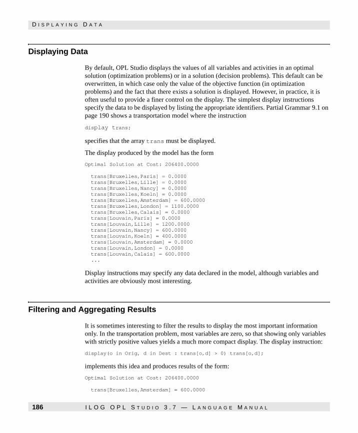
D I S P L A Y I N G D A T A
Displaying Data
By default, OPL Studio displays the values of all variables and activities in an optimal solution (optimization problems) or in a solution (decision problems). This default can be overwritten, in which case only the value of the objective function (in optimization problems) and the fact that there exists a solution is displayed. However, in practice, it is often useful to provide a finer control on the display. The simplest display instructions specify the data to be displayed by listing the appropriate identifiers. Partial Grammar 9.1 on page 190 shows a transportation model where the instruction
display trans;
specifies that the array trans must be displayed.
The display produced by the model has the form
Optimal Solution at Cost: 206400.0000
trans[Bruxelles,Paris] = 0.0000 trans[Bruxelles,Lille] = 0.0000 trans[Bruxelles,Nancy] = 0.0000 trans[Bruxelles,Koeln] = 0.0000 trans[Bruxelles,Amsterdam] = 600.0000 trans[Bruxelles,London] = 1100.0000 trans[Bruxelles,Calais] = 0.0000 trans[Louvain,Paris] = 0.0000 trans[Louvain,Lille] = 1200.0000 trans[Louvain,Nancy] = 600.0000 trans[Louvain,Koeln] = 400.0000 trans[Louvain,Amsterdam] = 0.0000 trans[Louvain,London] = 0.0000 trans[Louvain,Calais] = 600.0000 ...
Display instructions may specify any data declared in the model, although variables and activities are obviously most interesting.
Filtering and Aggregating Results
It is sometimes interesting to filter the results to display the most important information only. In the transportation problem, most variables are zero, so that showing only variables with strictly positive values yields a much more compact display. The display instruction:
display(o in Orig, d in Dest : trans[o,d] > 0) trans[o,d];
implements this idea and produces results of the form:
Optimal Solution at Cost: 206400.0000
trans[Bruxelles,Amsterdam] = 600.0000
186 I L O G O P L S T U D I O 3 . 7 — L A N G U A G E M A N U A L
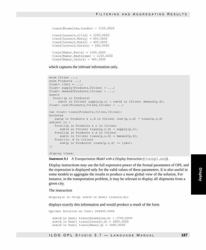
Disp
lay
F I L T E R I N G A N D A G G R E G A T I N G R E S U L T S
trans[Bruxelles,London] = 1100.0000
trans[Louvain,Lille] = 1200.0000 trans[Louvain,Nancy] = 600.0000 trans[Louvain,Koeln] = 400.0000 trans[Louvain,Calais] = 600.0000
trans[Namur,Paris] = 1500.0000 trans[Namur,Amsterdam] = 1100.0000 trans[Namur,Calais] = 400.0000
which captures the relevant information only.
Statement 9.1
Statement 9.1 A Transportation Model with a Display Instruction (transp1.mod).
Display instructions may use the full expressive power of the formal parameters of OPL and the expression is displayed only for the valid values of these parameters. It is also useful in some models to aggregate the results to produce a more global view of the solution. For instance, in the transportation problem, it may be relevant to display all shipments from a given city.
The instruction
display(o in Orig) sum(d in Dest) trans[o,d];
displays exactly this information and would produce a result of the form
Optimal Solution at Cost: 206400.0000
sum(d in Dest) trans[Bruxelles,d] = 1700.0000 sum(d in Dest) trans[Louvain,d] = 2800.0000 sum(d in Dest) trans[Namur,d] = 3000.0000
enum Cities ...; enum Products ...; float+ limit = ...; float+ supply[Products,Cities] = ...; float+ demand[Products,Cities] = ...; assert forall(p in Products) sum(o in Cities) supply[p,o] = sum(d in Cities) demand[p,d];float+ cost[Products,Cities,Cities] = ...;
var float+ trans[Products,Cities,Cities]; minimize sum(p in Products & o,d in Cities) cost[p,o,d] * trans[p,o,d]subject to { forall(p in Products & o in Cities) sum(d in Cities) trans[p,o,d] = supply[p,o]; forall(p in Products & d in Cities) sum(o in Cities) trans[p,o,d] = demand[p,d]; forall(o, d in Cities) sum(p in Products) trans[p,o,d] <= limit; };
display trans;
I L O G O P L S T U D I O 3 . 7 — L A N G U A G E M A N U A L 187

C O M P U T I N G D E R I V E D R E S U L T S
Computing Derived Results
The display instructions can in fact be interleaved with data declarations, as in
float+ transOrig[o in Orig] = sum(d in Dest) trans[o,d]; display transOrig;
These instructions produce essentially the same result as the instruction
display(o in Orig) sum(d in Dest) trans[o,d];
presented earlier. There are only syntactic differences in the result, which now becomes
Optimal Solution at Cost: 206400.0000
transOrig[Bruxelles] = 1700.0000 transOrig[Louvain] = 2800.0000 transOrig[Namur] = 3000.0000
These data declarations can also be browsed inside OPL Studio and are thus interesting in their own right.
Displaying Tuples
Another interesting feature of OPL is its ability to display tuples. For instance, the display instruction
display(d in Dest) <trans[Namur,d],trans[Namur,d].rc>;
displays the transportation variables and the corresponding reduced costs of the variables whose origin is Namur.
The result of this display expression is as follows:
Optimal Solution at Cost: 206400.0000
<trans[Namur,Paris],trans[Namur,Paris].rc> = <1500.0000,0.0000><trans[Namur,Lille],trans[Namur,Lille].rc> = <0.0000,2.0000><trans[Namur,Nancy],trans[Namur,Nancy].rc> = <0.0000,2.0000><trans[Namur,Koeln],trans[Namur,Koeln].rc> = <0.0000,1.0000><trans[Namur,Amsterdam],trans[Namur,Amsterdam].rc> = <1100.0000,0.0000><trans[Namur,London],trans[Namur,London].rc> = <0.0000,5.0000><trans[Namur,Calais],trans[Namur,Calais].rc> = <400.0000,0.0000>
Displaying Intermediate Results
For constraint programming and scheduling applications, OPL Studio displays the values of the objective function found in intermediate solutions. It is also possible to display
188 I L O G O P L S T U D I O 3 . 7 — L A N G U A G E M A N U A L

Disp
lay
F O R M A T T E D O U T P U T
additional results by using the onSolution instruction, which may include all the display instructions encountered so far.
For instance, for the house problem described in Chapter 2, A Short Tour of OPL, adding the instructions
onSolution { display a; }
would display the activities each time a solution is found.
Formatted Output
In addition to the display statement, OPL also supports formatted output statements
similar to C++ streams. The excerpt
int a = -12; float b = 1000000000; solve{}; cout <<‘[‘<< a << ‘]’ << endl; cout <<‘[‘<< setWidth(8) << setAdjustField(adjustLeft) << a << ‘]’ <<endl;cout <<‘[‘<< setWidth(8) << setAdjustField(adjustRight)<< a << ‘]’ <<endl;cout <<‘[‘<< setWidth(8) << setAdjustField(adjustInternal)<< a << ‘]’ <<endl;cout <<‘[‘<< setFloatField(fixed) << b << ‘]’ <<endl;cout <<‘[‘<< setFloatField(scientific) << b << ‘]’ <<endl;cout <<‘[‘<< setFloatField(fixed) << setPrecision(8) << b << ‘]’ <<endl;cout <<‘[‘<< setFloatField(scientific) << setPrecision(8) << b << ‘]’ <<endl;
produces the output
[-12] [-12 ] [ -12] [- 12] [1000000000.0000] [1.0000e+09] [1000000000.00000000] [1.00000000e+09]
with cout statements to print out an integer and a floating point number. It illustrates five different manipulators to format the output. The endl manipulator introduces a line feed in the output stream. setWidth(n) specifies that n characters must be written out. If fewer characters are available, padding is carried out with blanks. The setAdjustField manipulator affects the adjustment of the output. It can be one of adjustLeft, adjustRight or adjustInternal. For the first two, the padding is added to the left, or to the right. The third one pads the output between the sign and the first digit. The setFloatField manipulator affects the notation for floating point values that can be either
I L O G O P L S T U D I O 3 . 7 — L A N G U A G E M A N U A L 189

F O R M A T T E D O U T P U T
fixed point or scientific. The setPrecision(n) manipulator affects the number of digits after the decimal point.
Partial Grammar 9.1
Partial Grammar 9.1 The Syntax of the Display Instructions
Finally, it is possible to define new output streams tied to files. This can be achieved with the ofile statement as shown in
ofile f1("f1.txt"); int a = 1; var int x in 0..10; f1 << a << endl; solve { x = a + 1}; f1 << ‘[‘<< x << ‘]’ << endl;
Notice that the stream declaration and the stream output instructions can appear anywhere in the model statement. The complete syntax for the display section is listed in Partial Grammar 9.1 on page 190.
Display → display DisExpr;
→ display ( ListParameter ) DisExpr;
→ Type Id Subscripts = EltInit;
→ ofile Id ( Expr ) ;
→ cout << StreamOut { << StreamOut };
→ Composite << StreamOut {<< StreamOut };
DisExpr → Expr
→ <Expr+>
StreamOut → endl
setPrecision ( Expr )
setWidth ( Expr )
setFloatField ( FFManip )
setadjustField ( AFManip )
FFManip fixed | scientific
AFManip adjustLeft | adjustRight | adjustInternal
OnSolution → OnSolution { { Display } }
190 I L O G O P L S T U D I O 3 . 7 — L A N G U A G E M A N U A L

Disp
lay
F O R M A T T E D O U T P U T
I L O G O P L S T U D I O 3 . 7 — L A N G U A G E M A N U A L 191

F O R M A T T E D O U T P U T
192 I L O G O P L S T U D I O 3 . 7 — L A N G U A G E M A N U A L

C H A P T E R
Alg
orith
mic S
etting
s
10
Algorithmic Settings
This chapter describes a number of algorithmic settings that can be used to control the OPL implementation. For linear and mixed integer programming problems, the OPL implementation is based on CPLEX [25], a state-of-art mathematical programming software, and users can control the CPLEX parameter and algorithmic settings.
I L O G O P L S T U D I O 3 . 7 — L A N G U A G E M A N U A L 193

M A T H E M A T I C A L P R O G R A M M I N G
Mathematical Programming
This section reviews the algorithmic setting for mathematical programming in OPL, including the underlying algorithms, priorities and branching directions, and the CPLEX parameters.
Mixed Integer Programming Algorithms
OPL supports two default algorithms for integer programming and mixed integer programming: the CPLEX MIP algorithm and a branch and bound algorithm, called SOLVER MIP, that uses a cooperation between a simplex algorithm and constraint-based domain reduction. By default, when OPL recognizes a (mixed) integer program, OPL applies the CPLEX MIP algorithm and ignores the specified search procedure (if any). This default can be overwritten, either in OPL Studio or by using the declaration
setting MIPmethod = SOLVERmip;
For integer programs, OPL also supports a default algorithm not using the linear relaxation. This algorithm is accessible by using the declaration
setting MIPmethod = SOLVER;
Priorities and Branching Directions
In OPL you can set priorities and branching directions on integer variables. These directives are taken into account by the CPLEX MIP algorithm and are ignored by the SOLVER MIP algorithm. Priorities must be non-negative integers and variables with the highest priority are selected first for branching in the CPLEX MIP algorithm. The possible branching directions in OPL are branchDirLow, branchDirUp, and branchDirGlobal. The first two have their obvious meanings, while the third one lets the underlying algorithm determine the branching direction. The node corresponding to the specified branching direction is selected first in the CPLEX MIP algorithm when there is a tie for all the other criteria.
Statement 10.1 on page 195 enhances the knapsack model of Statement 2.10 on page 44 with priorities based on a simple heuristic and with branching directions.
Note: You should always place the instruction setting mipsearch before the maximize or minimize instruction. In other words, the setting block must precede the optimization block.
194 I L O G O P L S T U D I O 3 . 7 — L A N G U A G E M A N U A L

Alg
orith
mic S
etting
s
M A T H E M A T I C A L P R O G R A M M I N G
The instruction
setting mipsearch { forall(j in Columns) { setPriority(x[j],c[j]/maxCoef[j]); setBranchingDirection(x[j],branchDirLow); } };
associates a priority c[j]/maxCoef[j] and a branching direction branchDirLow with each variable x[j].
Statement 10.1
Statement 10.1 The Knapsack Problem with Priorities and Branching Directions (Knapsackp.mod).
CPLEX Parameters
It is also possible to specify the CPLEX parameters within OPL. This feature is documented in the OPL Studio User’s Manual and is not discussed here. Let us just mention a few facts. First, users can choose between several linear programming algorithms by using the OPL parameter LPmethod. For instance, the setting
setting LPmethod = barrier;
tells the OPL implementation to use CPLEX barrier. Other possible values for LPmethod are primal, dual, barrierPrimal, barrierDual, networkPrimal, and networkDual. Second, the syntax of the settings is depicted in Partial Grammar 10.1 on page 197. The value of the settings are, in general, integers, floats, and strings and each
int nbRows = ...; int nbColumns = ...; range Rows 1..nbRows; range Columns 1..nbColumns; int b[Rows] = ...; int c[Columns] = ...; int coef[Rows,Columns] = ...; int maxValue = max(i in Rows) b[i]; int maxCoef[j in Columns] = max(i in Rows) coef[i,j];
var int x[Columns] in 0..maxValue;
setting mipsearch { forall(j in Columns) { setPriority(x[j],c[j]/maxCoef[j]); setBranchingDirection(x[j],branchDirLow); } }; maximize sum(j in Columns) c[j] * x[j] subject to { forall( i in Rows ) sum(j in Columns) coef[i,j] * x[j] <= b[i]; };
I L O G O P L S T U D I O 3 . 7 — L A N G U A G E M A N U A L 195
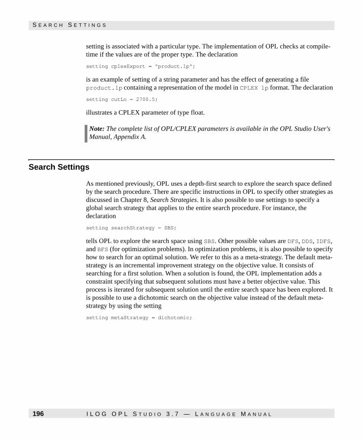
S E A R C H S E T T I N G S
setting is associated with a particular type. The implementation of OPL checks at compile-time if the values are of the proper type. The declaration
setting cplexExport = "product.lp";
is an example of setting of a string parameter and has the effect of generating a file product.lp containing a representation of the model in CPLEX lp format. The declaration
setting cutLo = 2700.5;
illustrates a CPLEX parameter of type float.
Search Settings
As mentioned previously, OPL uses a depth-first search to explore the search space defined by the search procedure. There are specific instructions in OPL to specify other strategies as discussed in Chapter 8, Search Strategies. It is also possible to use settings to specify a global search strategy that applies to the entire search procedure. For instance, the declaration
setting searchStrategy = SBS;
tells OPL to explore the search space using SBS. Other possible values are DFS, DDS, IDFS, and BFS (for optimization problems). In optimization problems, it is also possible to specify how to search for an optimal solution. We refer to this as a meta-strategy. The default meta- strategy is an incremental improvement strategy on the objective value. It consists of searching for a first solution. When a solution is found, the OPL implementation adds a constraint specifying that subsequent solutions must have a better objective value. This process is iterated for subsequent solution until the entire search space has been explored. It is possible to use a dichotomic search on the objective value instead of the default meta-strategy by using the setting
setting metaStrategy = dichotomic;
Note: The complete list of OPL/CPLEX parameters is available in the OPL Studio User's Manual, Appendix A.
196 I L O G O P L S T U D I O 3 . 7 — L A N G U A G E M A N U A L

Alg
orith
mic S
etting
s
S Y N T A X
Syntax
The syntax of settings is depicted in Partial Grammar 10.1.
Partial Grammar 10.1
Partial Grammar 10.1 The Syntax of Settings
SettingDecl → setting Setting+
Setting → Id = Integer
→ Id = Float
→ Id = String
→ Id = Id
→ mipsearch MIPSetting
MIPSetting → forall (ListParameter) MIPSetting
→ if Equivalence then MIPSetting [else MIPSetting] endif
→ { MIPSetting {; MIPSetting}}
→ setPriority ( Composite, Expr)
→ setBranchingDirection ( Composite, BranchingDirection)
BranchingDirection → branchDirLow
→ branchDirUp
→ branchDirGlobal
I L O G O P L S T U D I O 3 . 7 — L A N G U A G E M A N U A L 197

S Y N T A X
198 I L O G O P L S T U D I O 3 . 7 — L A N G U A G E M A N U A L

C H A P T E R
Datab
ases
11
Databases
This chapter describes how to interact with one or several relational databases in OPL. Relational databases can be read, written, and updated in OPL using traditional SQL queries. This chapter reviews these concepts in detail.
Database Connection
The database operations in OPL all refer to a database connection. The instruction
DBconnection db("odbc","DBPEOPLE//");
establishes a connection db to an odbc database whose name is "DBPEOPLE//". The connection db should be viewed as a handle on the database. Note that it is possible in OPL to connect to several databases within the same model. We often abuse language in this chapter and confuse the database connection with the database itself.
I L O G O P L S T U D I O 3 . 7 — L A N G U A G E M A N U A L 199

R E A D I N G F R O M A D A T A B A S E
Reading From a Database
In OPL, database relations can be read into sets. For instance, the instructions
struct People { string name; string email; int age; }; {People} Persons from DBread(db,"select NAME,EMAIL,AGE from PEOPLE");
illustrate how to initialize a set of records from the relation PEOPLE in database db while the instruction
{string} Names from DBread(db,"select NAME from PEOPLE");
illustrates how to initialize a set of strings. In both cases, the DBread instruction inserts an element into the set for each tuple of the relations. There are two important conventions adopted by OPL:
1. The resulting set must be a set of integers, of floats, of strings, or a set of records whose elements are integers, floats, or strings.
2. In the case of records, the columns of the database tuples are mapped by position to the field of the OPL records. For instance, in the above query, column NAME was mapped into field name and so on.
Note that OPL does not parse the query: it simply sends the string to the database system that has full responsibility for handling it. As a consequence, the syntax and the semantics of these queries is outside the scope of this book and users should consult the appropriate manual for more information. It is also possible to implement conditional queries in OPL. Consider the instructions
struct People { string name; string email; int age; }; int age = 30; {People} Persons from DBread(db,"select NAME,EMAIL,AGE from PEOPLE where AGE <= ?")(age);
These instructions produce a set of persons not older than 30. The query contains a placeholder whose value is given by an expression in between the parentheses. Of course, it is possible to have several placeholders as in
struct People { string name; string email; int age; } int age = 30; string dept = "marketing"; {People} Persons from DBread(db,"select NAME,EMAIL,AGE from PEOPLE where AGE <= ? and DEPT = ?")(age,dept);
which selects only those persons not older than 30 in the marketing department. Note that, once again, the syntax of placeholders may differ from one database system to another and users should consult the appropriate user's manual of their specific database for more information. OPL also makes it possible to replace the positional mapping between columns and fields by a symbolic mapping. The query
struct People {
200 I L O G O P L S T U D I O 3 . 7 — L A N G U A G E M A N U A L

U P D A T I N G A D A T A B A S E
Datab
ases
string email; string name; int age; }; int age = 30; {People} Persons from DBread(db,"select NAME,EMAIL,AGE from PEOPLE where AGE <= ?")(age) DBmapping {0 -> name; 1 -> email; 2 -> age;};
Note first that the order of fields name and email was swapped in the record definition. The mapping rules then specify that field name is to be mapped onto column 0 (i.e., NAME), field email onto column 1 (i.e., EMAIL), and field age onto column 2 (i.e., AGE), where the column order is specified by the select instruction.
Updating a Database
The updating and writing of a database mostly follows the same lines, although the asymmetry of SQL (e.g., the fact that placeholders are used to insert values) makes the syntax slightly non-uniform (i.e., there is no symbolic mapping).
The instructions
struct People { string name; string email; int age; int dept; }; {People} Persons = ...; DBupdate(db,"insert into PEOPLE (NAME,EMAIL,AGE,DEPT) values (?,?,?,?)")(Persons);
illustrates how to add the set of records Persons into the database relation PEOPLE. OPL automatically maps the fields of the records into the placeholders of the query. Because placeholders are used in SQL in these queries, there is no symbolic mapping possible. It is also possible to delete elements from a database. For instance, the instruction
{string} NamesToDelete = ...; DBupdate(db,"delete from PEOPLE where NAME = ? )(NamesToDelete);
deletes from relation PEOPLE all the tuples whose names are in NamesToDelete.
Other Operations
Finally, the instruction DBexecute makes it possible to execute operations such as creating and deleting tables. For instance, the instructions depicted in Statement 11.1 creates a table,
I L O G O P L S T U D I O 3 . 7 — L A N G U A G E M A N U A L 201

A C O M P L E T E E X A M P L E
initializes it with a number of elements, and deletes it. As mentioned several times already, the syntax of the actual queries may differ from one database system to another.
Statement 11.1
Statement 11.1 A Sequence of Database Instructions.
A Complete Example
Statement 11.2 on page 203 reconsiders the house problem once again. In this statement, the input data is read from a database and the results are written in the database as well. The instruction
DBconnection db"odbc","HOUSE//");
establishes the connection with the database. The next two instructions
struct TaskDuration { string Task; int duration; }; struct Schedule { string task; int startTime; int endTime; };
declares two record types to read from, and write into, the database. The database contains a binary relation storing the name of a task and its duration and the result will be a ternary relation storing the name of a task and its start- and end-dates.
The instructions
{TaskDuration} td from DBread(db,"select NAME,DURATION from HTASK"); {string} Tasks = { t | <t,d> in td }; int duration[Tasks]; initialize forall(<t,d> in td) duration[t] = d;
read the database and initializes the set of tasks (Tasks) and the array duration. In a first step, a set of records is read. In the second step, the set of tasks is computed by projection and the array of durations is declared and initialized.
The body of the statement is defined as in the previous statements for this problem and should not raise any difficulty. The instructions
DBconnection db("odbc","MYDB//"); struct Person { string name; int age; }; DBexecute(db,"create table PERSONS (NAME string,AGE integer)"); {Person} Persons = { <"McGuire",49>, <"McFarlan",52> }; DBupdate(db,"insert into PERSONS (NAME,AGE) values (?,?)")(Persons); {Person} See from DBread(db,"select NAME,AGE from PERSONS"); display See; DBexecute(db,"drop table PERSONS");
202 I L O G O P L S T U D I O 3 . 7 — L A N G U A G E M A N U A L

A C O M P L E T E E X A M P L E
Datab
ases
{Schedule} resultSet = { <t,a[t].start,a[t].end> | t in Tasks }; DBexecute(db, "create table sched (task string, startTime integer, endTime integer)");DBupdate(db, "insert into sched (task, startTime, endTime) values (?, ?, ?)")(resultSet);
write the result in the database. The first instruction collects all the results in the set resultSet. The second instruction creates a new table in the database to store the results and the third instruction inserts the set resultSet in the database.
Statement 11.2
Statement 11.2 The House Problem with a Database (house2db.mod).
DBconnection db("odbc","HOUSE//"); struct TaskDuration { string Task; int duration; }; struct Schedule { string task; int startTime; int endTime; };
{TaskDuration} td from DBread(db,"select NAME,DURATION from HTASK"); {string} Tasks = { t | <t,d> in td }; int duration[Tasks]; initialize forall(<t,d> in td) duration[t] = d;
scheduleHorizon = 30; Activity a[t in Tasks](duration[t]); DiscreteResource budget(29000); minimize a["moving"].end subject to { a["masonry"] precedes a["carpentry"]; a["masonry"] precedes a["plumbing"]; a["masonry"] precedes a["ceiling"]; a["carpentry"] precedes a["roofing"]; a["ceiling"] precedes a["painting"]; a["roofing"] precedes a["windows"]; a["roofing"] precedes a["facade"]; a["plumbing"] precedes a["facade"]; a["roofing"] precedes a["garden"]; a["plumbing"] precedes a["garden"]; a["windows"] precedes a["moving"]; a["facade"] precedes a["moving"]; a["garden"] precedes a["moving"]; a["painting"] precedes a["moving"]; capacityMax(budget,0,15,20000); forall(t in Tasks) a[t] consumes(1000*duration[t]) budget; };
{Schedule} resultSet = { <t,a[t].start,a[t].end> | t in Tasks }; DBexecute(db, "create table sched (task string, startTime integer, endTime integer)"); DBupdate(db, "insert into sched (task, startTime, endTime) values (?, ?, ?)")(resultSet);
I L O G O P L S T U D I O 3 . 7 — L A N G U A G E M A N U A L 203

S Y N T A X
Syntax
The syntax of database operations is depicted in Partial Grammar 11.1.
Partial Grammar 11.1
Partial Grammar 11.1 The Syntax of Database Operations
DBDecl → DBconnectionDecl
→ DBupdateDecl
→ DBexecuteDecl
DBconnectionDecl → DBconnection Id (String, String)
DBreadDecl → DBread (Id, String) [PlaceHolders] [InputMap]
PlaceHolders → (ListExpr)
InputMap → DBmapping {InputMap*}
InputMapping → Integer -> Id
DBupdateDecl → DBupdate (Id, String) ( ListExpr )
DBexecuteDecl → DBexecute (Id, String)
204 I L O G O P L S T U D I O 3 . 7 — L A N G U A G E M A N U A L

C H A P T E R
Sp
readsh
eet
12
Spreadsheets
This brief chapter describes how to read from a spreadsheet in OPL. The syntax of spreadsheet operations is depicted in Partial Grammar 12.1 on page 207.
Spreadsheet Connection
The spreadsheet operations in OPL all refer to a spreadsheet connection. The instruction
SheetConnection sheet("transport.xls");
establishes a connection sheet to a spreadsheet whose name is ''transport.xls''. The connection sheet should be viewed as a handle on the spreadsheet. Note that it is possible in OPL to connect to several spreadsheets within the same model. We often abuse language in this chapter and confuse the spreadsheet connection with the spreadsheet itself.
I L O G O P L S T U D I O 3 . 7 — L A N G U A G E M A N U A L 205

R E A D I N G F R O M A S P R E A D S H E E T
Reading From a Spreadsheet
In OPL, spreadsheet ranges can be read into multi-dimensional arrays or sets. For instance, the instructions
string city[0..2] from SheetRead(sheet,"C2:E2"); string product[0..2] from SheetRead(sheet,"B3:B5"); float cost[0..2,0..2] from SheetRead(sheet,"C3:E5");
illustrate how to initialize two one-dimensional arrays of strings, i.e., city and product, and one two-dimensional array of floats. Of course, OPL makes sure that the types of the spreadsheet and the types of OPL data structures agree. The instructions
{string} Cities from SheetRead(sheet,"C2:E2"); {string} Products from SheetRead(sheet,"B3:B5"); float ocost[Products,Cities] from SheetRead(sheet,"C3:E5");
illustrate how to initialize sets of strings from the same cells and how to initialize a 2-dimensional array ranging over these sets. Note also that the ranges specified can be names from within the spreadsheet.
Writing to a Spreadsheet
In OPL, multi-dimensional arrays and scalars can be written to a range of cells within a spreadsheet. For instance, the instructions
SheetConnection sheet("test.xls"); float costF[0..2, 0..2] from SheetRead(sheet, "C3:E5"); SheetWrite(sheet,"G3:I5")(costF);
copy the contents of the range "C3:E5" to a two dimensional array of floating point values and write the same array back into the spreadsheet in the range denoted by "G3:I5". The ranges used in the range specification must conform to the actual spreadsheet, i.e., they can be fixed ranges or named ranges. The objects written to the spreadsheet can be integers, floating point values or strings. By default, OPL opens a SheetConnection in read write mode. However, under certain circumstances, it might be desirable to open the connection in read-only mode. This can be achieved with the statement
SheetConnection sheet("transport.xls",1);
since the optional second argument is interpreted as a boolean value specifying whether the sheet is opened read-only or not.
206 I L O G O P L S T U D I O 3 . 7 — L A N G U A G E M A N U A L

Sp
readsh
eet
W R I T I N G T O A S P R E A D S H E E T
Partial Grammar 12.1
Partial Grammar 12.1 The Syntax of Spreadsheet Operations.
SheetDecl → SheetConnectionDecl
SheetConnectionDecl → SheetConnection Id [(String, [Expr])
SheetReadDecl → SheetRead (Id, String)
SheetWriteDecl → SheetWrite (Id, String) (Expr)
I L O G O P L S T U D I O 3 . 7 — L A N G U A G E M A N U A L 207

W R I T I N G T O A S P R E A D S H E E T
208 I L O G O P L S T U D I O 3 . 7 — L A N G U A G E M A N U A L

Part II


The Application Areas
This part applies OPL in three application areas: linear and integer programming, constraint programming, and scheduling.
I L O G O P L S T U D I O 3 . 7 — L A N G U A G E M A N U A L 211

212 I L O G O P L S T U D I O 3 . 7 — L A N G U A G E M A N U A L

C H A P T E R
Lin
ear and
Integ
er P
rog
ramm
ing
13
Linear and Integer Programming
This chapter studies the application of OPL to linear programming, integer programming, mixed-integer linear programming, and piecewise-linear programming.
Linear Programming
Linear programming consists of optimizing a linear function subject to linear constraints over real variables. As mentioned earlier, large instances of linear programs can be solved efficiently. This section reviews how to solve linear programs in OPL.
A Production Problem
Consider again the production planning problem of the section Records on page 38. The model is depicted again in Table 13.1 on page 218 and the instance data is shown in Table 13.2 on page 218. The model aims at minimizing the production cost for a number of products while satisfying customer demand. Each product can be produced either inside the company or outside, at a higher cost. The inside production is constrained by the company's resources, while outside production is considered unlimited. The model first declares the products and the resources. The data consists of the description of the products, i.e., the demand, the inside and outside costs, and the resource consumption, and the capacity of the various resources. The variables for this problem are the inside and outside production for each product.
I L O G O P L S T U D I O 3 . 7 — L A N G U A G E M A N U A L 213

L I N E A R P R O G R A M M I N G
For these statements, OPL returns the optimal solution
Optimal Solution with Objective Value 372.0000 inside[kluski] = 40.0000 inside[capellini] = 0.0000 inside[fettucine] = 0.0000
outside[kluski] = 60.0000 outside[capellini] = 200.0000 outside[fettucine] = 300.0000
A Multi-Period Production Planning Problem
Large linear-programming problems are often obtained from simpler ones by generalizing them along one or more dimensions. A typical extension of production-planning problems is to consider several production periods and to include inventories in the model. This section presents a multi-period production planning model that generalizes the model of the previous section.
Statement 13.1
Statement 13.1 A Production-Planning Problem (production.mod).
Statement 13.2
Statement 13.2 Instance Data for Production-Planning Problem (production.dat).
The main generalization is to consider the demand for the products over several periods and to allow the company to produce more than the demand in a given period. Of course, there is an inventory cost associated with storing the additional production. Statement 13.3 on
enum Products ...; enum Resources ...; float+ consumption[Products,Resources] = ...; float+ capacity[Resources] = ...; float+ demand[Products] = ...; float+ insideCost[Products] = ...; float+ outsideCost[Products] = ...;
var float+ inside[Products]; var float+ outside[Products];
minimize sum(p in Products) (insideCost[p]*inside[p] + outsideCost[p]*outside[p]) subject to { forall(r in Resources) sum(p in Products) consumption[p,r] * inside[p] <= capacity[r]; forall(p in Products) inside[p] + outside[p] >= demand[p]; };
Products = { kluski capellini fettucine }; Resources = { flour eggs }; consumption = [[0.5 0.2] [0.4 0.4] [0.3 0.6]]; capacity = [20, 40]; demand = [100, 200, 300]; insideCost = [0.6, 0.8, 0.3]; outsideCost = [0.8, 0.9, 0.4];
214 I L O G O P L S T U D I O 3 . 7 — L A N G U A G E M A N U A L

Lin
ear and
Integ
er P
rog
ramm
ing
L I N E A R P R O G R A M M I N G
page 217 depicts the new model and Statement 13.4 on page 218 describes the instance data. Most of the model generalizes smoothly. For instance, the capacity constraints stated for all resources and all periods become
forall(r in Resources, t in Periods) sum(p in Products) consumption[r,p] * inside[p,t] <= capacity[r];
The most novel part of the statement is the constraint linking the demand, the inventory, and the production:
forall(p in Products, t in Periods) inv[p,t-1] + inside[p,t] + outside[p,t] = demand[p,t] + inv[p,t];
The constraint states that, for each product p and each period t, the inventory of period t-1 added to the production of period t is equated to the demand of period t plus the inventory of period t. Of course, the fact that the variables inv[p,t] are constrained to be nonnegative is critical to satisfying the demand and to disallow back orders. The objective function is also generalized to add the inventory costs. Note also the type declaration
struct Plan { float+ inside; float+ outside; float+ inv; };
and the display instructions
Plan plan[p in Products, t in Periods] = <inside[p,t],outside[p,t],inv[p,t]>; display plan;
which were added to produce a visually pleasing display. For example, on the instance data depicted in Figure 13.1 on page 239, OPL produces the optimal solution
Optimal Solution with Objective Value: 344.6667
plan[kluski,1] = <inside:0.0000,outside:120.0000,inv:110.0000> plan[kluski,2] = <inside:0.0000,outside:0.0000,inv:10.0000> plan[kluski,3] = <inside:40.0000,outside:0.0000,inv:0.0000> plan[capellini,1] = <inside:0.0000,outside:320.0000,inv:300.0000> plan[capellini,2] = <inside:0.0000,outside:0.0000,inv:100.0000> plan[capellini,3] = <inside:0.0000,outside:0.0000,inv:0.0000> plan[fettucine,1] = <inside:66.6667,outside:116.6667,inv:133.3333> plan[fettucine,2] = <inside:66.6667,outside:0.0000,inv:100.0000> plan[fettucine,3] = <inside:0.0000,outside:0.0000,inv:0.0000>
A Blending Problem
Blending problems are another typical application of linear programming. Consider the following problem. An oil company manufactures three types of gasoline: super, regular, and diesel. Each type of gasoline is produced by blending three types of crude oil: crude1, crude2, and crude3. Table 13.1 on page 218 depicts the sales price and the purchase price per barrel of the various products. The gasoline must satisfy some quality
I L O G O P L S T U D I O 3 . 7 — L A N G U A G E M A N U A L 215

L I N E A R P R O G R A M M I N G
criteria with respect to their lead content and their octane ratings, thus constraining the possible blendings. Table 13.2 on page 218 describes the relevant instance data. The company must also satisfy its customer demand, which is 3,000 barrels a day of super, 2,000 of regular, and 1,000 of diesel. The company can purchase 5,000 barrels of each type of crude oil per day and can process at most 14,000 barrels a day. In addition, the company has the option of advertising a gasoline, in which case the demand for this type of gasoline increases by ten barrels for every dollar spent. Finally, it costs four dollars to transform a barrel of oil into a barrel of gasoline. The model is depicted in Statement 13.5 on page 219 and the instance data is shown in Statement 13.6 on page 219. The model uses two sets of variables. Variable a[g] represents the amount spent in advertising gasoline g. Variable blend[o,g] represents the number of barrels of crude oil o used to produced gasoline g. The demand constraints
forall(g in Gasolines) sum(o in Oils) blend[o,g] = gas[g].demand + 10*a[g];
use both types of variables, since sum(o in Crudes) blend[o,g] represents the amount of gasoline g produced daily. The constraints
forall(o in Oils) sum(g in Gasolines) blend[o,g] <= oil[o].capacity;
capture the purchase limitations for each type of oil. The constraint
sum(o in Oils, g in Gasolines) blend[o,g] <= maxProduction;
enforces the capacity limitation on production. The constraints
forall(g in Gasolines) sum(o in Oils) (oil[o].octane - gas[g].octane) * blend[o,g] >= 0; forall(g in Gasolines) sum(o in Oils) (oil[o].lead - gas[g].lead) * blend[o,g] <= 0;
enforce the quality criteria for the gasoline. The objective function
sum(g in Gasolines, o in Oils) (gas[g].price - oil[o].price - prodCost) * blend[o,g] - sum(g in Gasolines) a[g]
has four parts: the sales price of the gasoline, the purchase cost of the crude oils, the production costs, and the adverting costs. The optimal solution for this problem is
Optimal Solution with Objective Value: 287750.0000 a[super] = 0.0000 a[regular] = 750.0000 a[diesel] = 0.0000 blend[Crude1,super] = 2000.0000 blend[Crude1,regular] = 2200.0000 blend[Crude1,diesel] = 800.0000 blend[Crude2,super] = 1000.0000 blend[Crude2,regular] = 4000.0000 blend[Crude2,diesel] = 0.0000 blend[Crude3,super] = 0.0000 blend[Crude3,regular] = 3300.0000 blend[Crude3,diesel] = 200.0000
216 I L O G O P L S T U D I O 3 . 7 — L A N G U A G E M A N U A L

Lin
ear and
Integ
er P
rog
ramm
ing
L I N E A R P R O G R A M M I N G
Statement 13.3
Statement 13.3 A Multi-Period Production-Planning Problem (mulprod.mod).
enum Products ...; enum Resources ...; int nbPeriods = ...; range Periods 1..nbPeriods; struct Plan { float+ inside; float+ outside; float+ inv; }; float+ consumption[Resources,Products] = ...; float+ capacity[Resources] = ...; float+ demand[Products,Periods] = ...; float+ inCost[Products] = ...; float+ outCost[Products] = ...; float+ inventory[Products] = ...; float+ invCost[Products] = ...;
var float+ inside[Products,Periods]; var float+ outside[Products,Periods]; var float+ inv[Products,0..nbPeriods];
minimize sum(p in Products, t in Periods) (inCost[p]*inside[p,t] + outCost[p]*outside[p,t] + invCost[p]*inv[p,t]) subject to { forall(r in Resources, t in Periods) sum(p in Products) consumption[r,p] * inside[p,t] <= capacity[r]; forall(p in Products, t in Periods) inv[p,t-1] + inside[p,t] + outside[p,t] = demand[p,t] + inv[p,t]; forall(p in Products) inv[p,0] = inventory[p]; }; Plan plan[p in Products, t in Periods] = <inside[p,t],outside[p,t],inv[p,t]>; display plan;
I L O G O P L S T U D I O 3 . 7 — L A N G U A G E M A N U A L 217

L I N E A R P R O G R A M M I N G
Statement 13.4
Statement 13.4 Instance Data for Multi-Period Production-Planning Problem (mulprod.dat)
Products = { kluski capellini fettucine }; Resources = { flour eggs }; nbPeriods = 3; consumption = [ [0.5, 0.4, 0.3], [0.2, 0.4, 0.6] ]; capacity = [20, 40]; demand = [ [10 100 50] [20 200 100] [50 100 100] ]; inventory = [0 0 0]; invCost = [0.1 0.2 0.1]; insideCost = [0.4, 0.6, 0.1]; outsideCost = [0.8, 0.9, 0.4];
Table 13.1 Prices for the Blending Problem.
Sales Price Purchase Price
super $ 70 crude1 $ 45
regular $ 60 crude2 $ 35
diesel $ 50 crude3 $ 25
Table 13.2 Octane and Lead Data for the Blending Problem.
Octane Rating Lead Content Octane Rating Lead Content
super ≥ 10 ≤ 1 crude1 12 0.5
regular ≥ 8 ≤ 2 crude2 6 2.0
diesel ≥ 6 ≤ 1 crude3 8 3.0
218 I L O G O P L S T U D I O 3 . 7 — L A N G U A G E M A N U A L

Lin
ear and
Integ
er P
rog
ramm
ing
L I N E A R P R O G R A M M I N G
Statement 13.5
Statement 13.5 An Oil-Blending Planning Problem (oil.mod).
Statement 13.6
Statement 13.6 Data for the Oil-Blending Planning Problem (oil.dat).
enum Gasolines ...; enum Oils ...; struct GasType { float+ demand; float+ price; float+ octane; float+ lead; };struct OilType { float+ capacity; float+ price; float+ octane; float+ lead; };
GasType gas[Gasolines] = ...; OilType oil[Oils] = ...; float+ maxProduction = ...; float+ prodCost = ...;
var float+ a[Gasolines]; var float+ blend[Oils,Gasolines];
maximize sum(g in Gasolines, o in Oils) (gas[g].price - oil[o].price - prodCost) * blend[o,g] - sum(g in Gasolines) a[g] subject to { forall(g in Gasolines) sum(o in Oils) blend[o,g] = gas[g].demand + 10*a[g]; forall(o in Oils) sum(g in Gasolines) blend[o,g] <= oil[o].capacity;
sum(o in Oils, g in Gasolines) blend[o,g] <= maxProduction;
forall(g in Gasolines) sum(o in Oils) (oil[o].octane - gas[g].octane) * blend[o,g] >= 0; forall(g in Gasolines) sum(o in Oils) (oil[o].lead - gas[g].lead) * blend[o,g] <= 0; };
Gasolines = { super regular diesel }; Oils = { crude1 crude2 crude3 }; gas = [ #<demand:3000 price:70 octane:10 lead:1># #<demand:2000 price:60 octane:8 lead:2># #<demand:1000 price:50 octane:6 lead:1>#]; oil = [ #<capacity:5000 price:45 octane:12 lead:0.5># #<capacity:5000 price:35 octane:6 lead:2># #<capacity:5000 price:25 octane:8 lead:3>#]; maxProduction = 14000; prodCost = 4;
I L O G O P L S T U D I O 3 . 7 — L A N G U A G E M A N U A L 219

L I N E A R P R O G R A M M I N G
Statement 13.7
Statement 13.7 A Multi-Product Transportation Model (transp1.mod).
Exploiting Sparsity
Statement 13.7 on page 220 gives again the transportation problem presented in the section Modeling Issues on page 145. This problem, known as a multi-commodity flow problem on a bipartite graph, is a classic transportation problem with the addition of a capacity constraint on the inter-cities connections. The model is, of course, not appropriate for large-scale transportation problems, where only a fraction of the cities are connected and a fraction of the products are sent along the connections. This section discusses how to exploit the sparsity of large-scale problems. OPL offers more support than other modeling languages in this respect, because it can use records and arrays indexed by arbitrary finite sets. The methodology for exploiting sparsity in OPL consists of mirroring, in the model, the structure of the application. This structure can be inferred from the objective function and the constraints of the application. For instance, the capacity constraint for the transportation application can be phrased as
"The products sent along any given connection may not exceed the given capacity."
This constraint helps identify two main concepts in the application. The first is the connection between two cities, which can be represented explicitly by a data type
struct Connection { Cities o; Cities d; };
to manipulate connections as first-class objects. The second fundamental concept is the transportation of a product along a connection, called a route in this section. Once again, this concept can be represented explicitly by a data type
struct Route { Connection e; Products p; };
enum Cities ...; enum Products ...; float+ limit = ...; float+ supply[Products,Cities] = ...; float+ demand[Products,Cities] = ...; assert forall(p in Products) sum(o in Cities) supply[p,o] = sum(d in Cities) demand[p,d]; float+ cost[Products,Cities,Cities] = ...; var float+ trans[Products,Cities,Cities]; minimize sum(p in Products & o,d in Cities) cost[p,o,d] * trans[p,o,d] subject to { forall(p in Products & o in Cities) sum(d in Cities) trans[p,o,d] = supply[p,o]; forall(p in Products & d in Cities) sum(o in Cities) trans[p,o,d] = demand[p,d]; forall(o, d in Cities) sum(p in Products) trans[p,o,d] <= limit; };
220 I L O G O P L S T U D I O 3 . 7 — L A N G U A G E M A N U A L

Lin
ear and
Integ
er P
rog
ramm
ing
L I N E A R P R O G R A M M I N G
to manipulate routes directly. The supply and demand constraints exhibit two other fundamental concepts: product suppliers (i.e., the association of a product and a city supplying it) and product consumers (i.e., the association of a product and a city consuming it). The data types
struct Supplier { Products p; Cities o; }; struct Customer { Products p; Cities d; };
may be used to represent them.
Once the concepts are identified, an appropriate data representation can be chosen so that the model can generate constraints efficiently. Of course, the user data is not necessarily expressed in this representation, but it is usually easy in OPL to transform the user data into an appropriate representation.
A good representation for this application consists of a set of connections, a set of routes, the cost of the routes, and the demand and supply information, e.g.,
{Route} Routes = ...; float+ cost[Routes] = ...; {Connection} Connections = { c | <c,p> in Routes }; {Supplier} Suppliers = { <p,c.o> | <c,p> in Routes }; float+ supply[Suppliers] = ...; {Customer} Customers = { <p,c.d> | <c,p> in Routes }; float+ demand[Customers] = ...;
I L O G O P L S T U D I O 3 . 7 — L A N G U A G E M A N U A L 221

L I N E A R P R O G R A M M I N G
Statement 13.8
Statement 13.8 A Sparse Multi-Product Transportation Model (transp3.mod).
Note that the connections, suppliers, and customers are derived automatically from the routes. It is also useful to derive the following data to simplify the constraint statement:
{Cities} orig[p in Products] = { c.o | <c,p> in Routes }; {Cities} dest[p in Products] = { c.d | <c,p> in Routes }; {Connection} CP[p in Products] = { c | <p,c> in Routes };
The objective function and the constraints can now be stated naturally. The objective function
"minimize the transportation costs along all routes"
is expressed elegantly as
minimize sum(r in Routes) cost[r] * trans[r]
enum Cities ...; enum Products ...;
struct Connection { Cities o; Cities d; }; struct Route { Connection e; Products p; }; struct Supplier { Products p; Cities o; }; struct Customer { Products p; Cities d; };
{Route} Routes = ...; {Connection} Connections = { c | <c,p> in Routes }; {Supplier} Suppliers = { <p,c.o> | <c,p> in Routes }; float+ supply[Suppliers] = ...; {Customer} Customers = { <p,c.d> | <c,p> in Routes }; float+ demand[Customers] = ...; float+ lim = ...; float+ cost[Routes] = ...; {Cities} orig[p in Products] = { c.o | <c,p> in Routes }; {Cities} dest[p in Products] = { c.d | <c,p> in Routes }; {Connection} CP[p in Products] = { c | <p,c> in Routes }; assert forall(p in Products) sum(o in orig[p]) supply[<p,o>] = sum(d in dest[p]) demand[<p,d>];
var float+ trans[Routes];
minimize sum(r in Routes) cost[r] * trans[r] subject to { forall(p in Products & o in orig[p]) sum(<o,d> in CP[p]) trans[< <o,d>,p>] = supply[<p,o>]; forall(p in Products & d in dest[p]) sum(<o,d> in CP[p]) trans[< <o,d>,p>] = demand[<p,d>]; forall(c in Connections) sum(<c,p> in Routes) trans[<c,p>] <= lim; };
222 I L O G O P L S T U D I O 3 . 7 — L A N G U A G E M A N U A L

Lin
ear and
Integ
er P
rog
ramm
ing
I N T E G E R P R O G R A M M I N G
The supply constraint, which can be phrased as
"for every product and every city shipping the product, the summation of all transportations from that city to a city where the product is in demand is equal to the supply of the product at the supplying city"
is formalized by
forall(p in Products & o in orig[p]) sum(<o,d> in CP[p]) trans[< <o,d>,p>] = supply[<p,o>];
The demand constraints are stated in a similar way. The capacity constraints are stated elegantly as
forall(c in Connections) sum(<c,p> in Routes) trans[< <c.o,c.d>,p>] <= lim;
This statement is efficient, since OPL retrieves the product from the routes in an efficient way when the connection is known. The complete model is shown in Statement 13.8 on page 222. Assume now that part of the user data is given by a relational table that contains tuples of the form <o,d,p,c> indicating that a connection between cities o and d transports product p at cost c. This data can be transformed into the representation used in Statement 13.8. The routes can be obtained as
{Route} Routes = { < <o,d>,p> | <p,o,d,c> in TableRoutes };
and the costs as
initialize { forall(<p,o,d,c> in TableRoutes) cost[< <o,d>,p>] = c; };
Both of these preprocessings are linear in the size of the table.
Integer Programming
Integer programming is the class of problems defined as the optimization of a linear function subject to linear constraints over integer variables. Integer programs are, in general, much harder to solve than linear programs and the size of integer programs that can be solved efficiently is much smaller than of linear programs. This section reviews a number of typical integer programs.
Set Covering
Consider selecting workers to build a house. The construction of a house can be divided into a number of tasks, each requiring a number of skills (e.g., plumbing or masonry). A worker may or may not perform a task, depending on skills. In addition, each worker can be hired
I L O G O P L S T U D I O 3 . 7 — L A N G U A G E M A N U A L 223

I N T E G E R P R O G R A M M I N G
for a cost that also depends on his qualifications. The problem consists of selecting a set of workers to perform all the tasks, while minimizing the cost. This is known as a set-covering problem. The key idea in modeling a set-covering problem as an integer program is to associate a 0/1 variable with each worker to represent whether the worker is hired. To make sure that all the tasks are performed, it is sufficient to choose at least one worker by task. This constraint can be expressed by a simple linear inequality.
Statement 13.9 describes a set-covering model for this problem and Statement 13.10 shows some instance data.
Statement 13.9
Statement 13.9 A Set-Covering Model (covering.mod).
Statement 13.10
Statement 13.10 Instance Data for the Set-Covering Model (covering.dat).
range Boolean 0..1; int nbWorkers = ...; range Workers 1..nbWorkers; enum Tasks ...; {Workers} qualified[Tasks] = ...; int cost[Workers] = ...;
var Boolean hire[Workers]; minimize sum(c in Workers) cost[c]*hire[c] subject to forall(j in Tasks) sum(c in qualified[j]) hire[c] >= 1; {Workers} crew = { c | c in Workers : hire[c] = 1 }; display crew;
Tasks = { masonry, carpentry, plumbing, ceiling, electricity, heating, insulation, roofing, painting, windows, facade, garden, garage, driveway, moving }; nbWorkers = 32; qualified = [ { 1 9 19 22 25 28 31 } { 2 12 15 19 21 23 27 29 30 31 32 } { 3 10 19 24 26 30 32 } { 4 21 25 28 32 } { 5 11 16 22 23 27 31 } { 6 20 24 26 30 32 } { 7 12 17 25 30 31 } { 8 17 20 22 23 } { 9 13 14 26 29 30 31 } { 10 21 25 31 32 } { 14 15 18 23 24 27 30 32 } { 18 19 22 24 26 29 31 } { 11 20 25 28 30 32 } { 16 19 23 31 } { 9 18 26 28 31 32 }]; cost = [1 1 1 1 1 1 1 1 2 2 2 2 2 2 2 3 3 3 3 4 4 4 4 5 5 5 6 6 6 7 8 9];
224 I L O G O P L S T U D I O 3 . 7 — L A N G U A G E M A N U A L

Lin
ear and
Integ
er P
rog
ramm
ing
I N T E G E R P R O G R A M M I N G
The first instruction in the model declares a range Boolean, a range for the workers and an enumerated type for the tasks. The instruction
{Workers} qualified[Tasks] = ...;
declares the workers qualified to perform a given task, i.e., qualified[t] is the set of workers able to perform task t. The problem variables
var Boolean hire[Workers];
indicate whether a worker is hired for the project.
The constraints
forall(t in Tasks) sum(w in qualified[t]) hire[w] >= 1
make sure that each task is covered by at least on worker. Note also the declaration
{workers} crew = {w | w in Workers: hire[w] = 1};
which collects all the hired workers in the set Crew to produce a more pleasing representation of the results. OPL returns the solution
Optimal Solution at Cost: 14 crew = {23, 25, 26};
for the instance data given above.
Warehouse Location
Warehouse location is another typical integer-programming problem. Consider a company that is considering a number of locations for building warehouses to supply its existing stores. Each possible warehouse has a fixed maintenance cost and a maximum capacity specifying how many stores it can support. In addition, each store can be supplied by only one warehouse and the supply cost to the store differs according to the warehouse selected. The application consists of choosing which warehouses to build and which of them should supply the various stores in order to minimize the total cost, i.e., the sum of the fixed and supply costs. The instance used in this section considers five warehouses and 10 stores. The fixed costs for the warehouses are all identical and equal to 30. Table 13.3 on page 226 depicts the transportation costs and the capacity constraints. The key idea in representing a warehouse-location problem as an integer program consists of using a 0-1 variable for each (warehouse, store) pair to represent whether a warehouse supplies a store. In addition, the model also associates a variable with each warehouse to indicate whether the warehouse is selected. Once these variables are declared, the constraints state that each store must be supplied by a warehouse, that each store can be supplied by only an open warehouse, and that each warehouse cannot deliver more stores than its allowed capacity. The most delicate aspect of the modeling is expressing that a warehouse can supply a store only when it is open. These constraints can be expressed by inequalities of the form
I L O G O P L S T U D I O 3 . 7 — L A N G U A G E M A N U A L 225

I N T E G E R P R O G R A M M I N G
supply[w,s] <= open[w]
which ensures that when warehouse w is not open, it does not supply store s. This follows from the fact that open[w] = 0 implies supply[w,s] = 0. In fact, these constraint can be combined with the capacity constraints to obtain
forall(w in Warehouses, s in Stores) sum(s in Stores) supply[s,w] <= capacity[w]*open[w];
This formulation implies that a closed warehouse has no capacity.
Table 13.3 Instance Data for the Warehouse-Location Problem
Bonn Bordeaux London Paris Rome
capacity 1 4 2 1 3
store1 20 24 11 25 30
store2 28 27 82 83 74
store3 74 97 71 96 70
store4 2 55 73 69 61
store5 46 96 59 83 4
store6 42 22 29 67 59
store7 1 5 73 59 56
store8 10 73 13 43 96
store9 93 35 63 85 46
store10 47 65 55 71 95
226 I L O G O P L S T U D I O 3 . 7 — L A N G U A G E M A N U A L

Lin
ear and
Integ
er P
rog
ramm
ing
I N T E G E R P R O G R A M M I N G
Statement 13.11 describes an integer program for the warehouse-location problem, and Statement 13.12 depicts some instance data.
Statement 13.11
Statement 13.11 A Warehouse-Location Model (warehouse.mod).
Statement 13.12
Statement 13.12 Data for the Warehouse-Location Model (warehouse.dat).
The statement declares the warehouses and the stores, the fixed cost of the warehouses, and the supply cost of a store for each warehouse. The problem variables
var Boolean supply[Stores, Warehouses]
represent which warehouses supply the stores, i.e., supply[s,w] is 1 if warehouse w supplies store s and zero otherwise.
range Boolean 0..1; int fixed = ...; enum Warehouses ...; int nbStores = ...; range Stores 0..nbStores-1; int capacity[Warehouses] = ...; int supplyCost[Stores,Warehouses] = ...;
var Boolean open[Warehouses]; var Boolean supply[Stores,Warehouses];
minimize sum(w in Warehouses) fixed * open[w] + sum(w in Warehouses, s in Stores) supplyCost[s,w] * supply[s,w] subject to { forall(s in Stores) sum(w in Warehouses) supply[s,w] = 1; forall(w in Warehouses, s in Stores) sum(s in Stores) supply[s,w] <= capacity[w]*open[w]; };
display open; {Stores} storesof[w in Warehouses] = { s | s in Stores : supply[s,w] }; display storesof;
fixed = 30; nbStores = 10; Warehouses = {Bonn Bordeaux London Paris Rome }; capacity = [1,4,2,1,3]; supplyCost = [ [20 24 11 25 30] [28 27 82 83 74] [74 97 71 96 70] [ 2 55 73 69 61] [46 96 59 83 4] [42 22 29 67 59] [ 1 5 73 59 56] [10 73 13 43 96] [93 35 63 85 46] [47 65 55 71 95]];
I L O G O P L S T U D I O 3 . 7 — L A N G U A G E M A N U A L 227

I N T E G E R P R O G R A M M I N G
The objective function
minimize sum(w in Warehouses) fixedCost * open[w] + sum(w in Warehouses, s in Stores) supplyCost[s,w] * supply[s,w]
expresses the goal that the model minimizes the fixed cost of the selected warehouses and the supply costs of the stores.
The constraint
forall(s in Stores) sum(w in Warehouses) supply[s,w] = 1
states that a store must be supplied by exactly one warehouse. The constraint
forall(w in Warehouses) sum(s in Stores) supply[s,w] <= capacity[w]*open[w];
expresses the capacity constraints for the warehouses and makes sure that a warehouse supplies a store only if the warehouse is open. For the instance data depicted in Statement 13.12 on page 227, OPL returns the optimal solution
Optimal Solution with Objective Value: 383
open[Bonn] = 1 open[Bordeaux] = 1 open[London] = 1 open[Paris] = 0 open[Rome] = 1 storesof[Bonn] = { 3 } storesof[Bordeaux] = { 8, 6, 5, 1 } storesof[London] = { 9, 7 } storesof[Paris] = { } storesof[Rome] = { 4, 2, 0 }
Fixed-Charge Problems
Fixed-charge problems are another classic application of integer programs. They resemble some of the production problems seen previously but differ in two respects: the production is an integer value (e.g., a factory must produce bikes or toys), and the factories need to rent (or acquire) some tools to produce some of the products. Consider the following problem. A company manufactures shirts, shorts, and pants. Each product requires a number of hours of labor and a certain amount of cloth, and the company has a limited capacity of both. In addition, all of these products can be manufactured only by renting an appropriate machine. The profit on the products (excluding the cost of renting the equipment) are also known. The company would like to maximize its profit.
228 I L O G O P L S T U D I O 3 . 7 — L A N G U A G E M A N U A L

Lin
ear and
Integ
er P
rog
ramm
ing
I N T E G E R P R O G R A M M I N G
Statement 13.13 shows a model for fixed charge problems, while Statement 13.14 gives some instance data.
Statement 13.13
Statement 13.13 A Fixed-Charge Model (fixed.mod).
Statement 13.14
Statement 13.14 Data for the Fixed-Charge Model (fixed.dat).
The integer program for this model uses two sets of variables: production variables and rental variables. A production variable produce[p] describes the production of product p; a rental variable rent[m] is a 0-1 variable representing whether machine m is rented. Most of the constraints are similar to traditional production problems and pose few difficulties. The most delicate aspect of the modeling is expressing that a product can be produced only if its equipment is rented.
enum Machines ...; enum Products ...; enum Resources ...; range Boolean 0..1;
int+ capacity[Resources] = ...; int MaxProduction = max(r in Resources) capacity[r]; int rentingCost[Machines] = ...;
struct ProductType { int profit; {Machines} machines; int use[Resources]; }; ProductType product[Products] = ...;
var Boolean rent[Machines]; var int produce[Products] in 0..MaxProduction;
maximize sum(p in Products) product[p].profit * produce[p] - sum(m in Machines) rentingCost[m] * rent[m] subject to { forall(r in Resources) sum(p in Products) product[p].use[r] * produce[p] <= capacity[r]; forall(p in Products, m in product[p].machines) produce[p] <= MaxProduction * rent[m]; };
Machines = { shirtM shortM pantM }; Products = { shirt shorts pants }; Resources = { labor cloth }; capacity = [150 160]; rentingCost = [200 150 100]; product = [ <6 {shirtM} [3 4]> <4 {shortM} [2 3]> <7 {pantM} [6 4]>];
I L O G O P L S T U D I O 3 . 7 — L A N G U A G E M A N U A L 229

I N T E G E R P R O G R A M M I N G
It is not possible to use the same idea as in the warehouse-location problem: e.g., a constraint
produce[p] <= rent[m]
is not correct, since produce[p] is not a Boolean variable in this model. One might be tempted to write
produce[p] <= produce[p] * rent[m]
but this constraint is not linear. The solution adopted in the model is to use an integer representing the maximal production of any product and write
produce[p] <= maxProduction * rent[m]
If machine m is rented, then the constraint is redundant, since maxProduction is chosen to be larger than produce[p]. Otherwise, the right-hand side is zero and product p cannot be manufactured. Note the data representation in this model.
The type
struct ProductType { int profit; {Machines} machines; int use[Resources]; };
clusters all data related to a product: its profit, the set of machines it requires, and the way it uses the resources. Note also the constraint
forall(p in Products, m in product[p].machines) produce[p] <= maxProduction * rent[m];
which features a forall statement that quantifies over each product and over each machine used by the product.
Search Procedures
Integer programs are generally solved using a branch-and-bound algorithm that uses a linear relaxation at each node of the search tree. When the CPLEX MIP algorithm is used, search procedures are ignored. The rest of this section thus assumes that a SOLVER MIP algorithm is used. OPL provides a number of predefined tools to let users specify their own search procedures. A traditional approach in integer programming is to design a search procedure that splits the domain of a variable in two parts and explores both parts nondeterministically. The splitting point is generally the value of the variable in the linear relaxation. Such a procedure can be implemented as follows:
while not isBound(x) do let v = simplexValue(x) in let l = floor(v) in let v = ceil(v) in try x <= l | x >= v endtry
230 I L O G O P L S T U D I O 3 . 7 — L A N G U A G E M A N U A L

Lin
ear and
Integ
er P
rog
ramm
ing
M I X E D I N T E G E R - L I N E A R P R O G R A M M I N G
This search procedure is supported directly by the instruction splitLow. The instruction splitUp is similar, except that the order of the alternatives in the try instruction is permuted. The instruction split is similar but the order is implementation-dependent. The instructions branch, branchLow, and branchUp generalize the split instructions to arrays of variables. For instance, assuming that x is a one-dimensional array of integer variables, the instruction branchLow(x) can be written as
while not isBound(x) do select(i in Index : not isBound(x[i])) splitLow(x[i]);
These branching instructions can also be applied to arrays of arbitrary dimensions. Of course, all the other constructs described in Chapter 7, Search can be used as well.
Mixed Integer-Linear Programming
Mixed integer-linear programs are linear programs in which some variables are required to take integer values, and arise naturally in many applications. The integer variables may come from the nature of the products (e.g., a machine may, or may not, be rented). Mixed integer-linear programs are solved using the same technology as integer programs (or vice-versa). For instance, a branch-and-bound algorithm can exploit the linear relaxation and its branching procedure is applied only to integer variables. Consider how to upgrade the production-planning problem in the section Records on page 38 to include a fixed charge for the products. Statement 13.15 on page 232 describes the new model and Statement 13.16 on page 232 describes the instance data.
I L O G O P L S T U D I O 3 . 7 — L A N G U A G E M A N U A L 231

M I X E D I N T E G E R - L I N E A R P R O G R A M M I N G
Statement 13.15
Statement 13.15 A Fixed-Charge Production Model (prodmilp.mod).
Statement 13.16
Statement 13.16 Data for the Fixed-Charge Production Model (prodmilp.dat.)
Note that the model now contains two types of variables: 0-1 variables that represent whether to rent a machine and production variables of type float+. The product data is enhanced with a field describing the required machine, while the new constraints are modeled as in the fixed-charge problem in Statement 13.13 on page 229.
range Boolean 0..1; enum Products ...; enum Resources ...; enum Machines ...; float+ maxProduction = ...; struct TypeProductData { float+ demand; float+ incost; float+ outcost; float+ use[Resources]; Machines machine; }; TypeProductData product[Products] = ...; float+ capacity[Resources] = ...; float+ rentCost[Machines] = ...;
var Boolean rent[Machines]; var float+ inside[Products]; var float+ outside[Products];
minimize sum(p in Products) (product[p].incost*inside[p] + product[p].outcost*outside[p]) + sum(m in Machines) rentCost[m] * rent[m] subject to { forall(r in Resources) sum(p in Products) product[p].use[r] * inside[p] <= capacity[r];
forall(p in Products) inside[p] + outside[p] >= product[p].demand;
forall(p in Products) inside[p] <= maxProduction * rent[product[p].machine]; };
Products = { kluski capellini fettucine }; Resources = { flour eggs }; Machines = { m1 m2 m3 }; rentCost = [20 10 5]; maxProduction = 100000; product = #[ kluski : <100 0.6 0.8 [0.5 0.2] m1> capellini : <200 0.8 0.9 [0.4, 0.4] m2> fettucine : <300 0.3 0.4 [0.3, 0.6] m3>]#; capacity = [20, 40];
232 I L O G O P L S T U D I O 3 . 7 — L A N G U A G E M A N U A L

Lin
ear and
Integ
er P
rog
ramm
ing
P I E C E W I S E L I N E A R P R O G R A M M I N G
On the instance data in Statement 13.16 on page 232, OPL returns the optimal solution
Optimal Solution with Objective Value: 378.3333
rent[m1] = 0 rent[m2] = 0 rent[m3] = 1
inside[kluski] = 0.0000 inside[capellini] = 0.0000 inside[fettucine] = 66.6667
outside[kluski] = 100.0000 outside[capellini] = 200.0000 outside[fettucine] = 233.3333
Piecewise Linear Programming
This section considers piecewise linear programs, which are also useful in simplifying the models for a variety of applications. Piecewise linear programs are in fact syntactic sugar for linear, integer, or mixed integer-linear programs. In other words, a piecewise linear program can always be transformed into a mixed integer linear program and, sometimes, into a linear program. This last case is particularly interesting from a computational standpoint. This section introduces piecewise linear programs using an inventory application. The company Sailco must determine how many sailboats to produce over four time periods. The demand for the four periods is known (40, 60, 75, 25) and, in addition, an inventory of ten boats is available initially. In each period, Sailco can produce 40 boats at a cost of $400 per boat. Additional boats can be produced at a cost of $450 per boat. The inventory cost is $20 per boat and per period. Statement 13.17 on page 234 describes a linear program for this application and Statement 13.18 on page 234 describes the instance data.
I L O G O P L S T U D I O 3 . 7 — L A N G U A G E M A N U A L 233

P I E C E W I S E L I N E A R P R O G R A M M I N G
Statement 13.17
Statement 13.17 A Simple Inventory Model (sailco.mod).
Statement 13.18
Statement 13.18 Data for the Simple Inventory Model (sailco.dat).
The key idea underlying this model is to use two sets of variables for describing the production: variables regulBoat[t] represent the number of boats built at the regular price ($400 in the instance data) for period t, while extraBoat[t] represents the number of extra boats, i.e., boats built at the higher price. The model also contains inventory variables. Most of the constraints are typical for inventory problems. In addition, the constraint
forall(t in Periods) regulBoat[t] <= capacity;
states that there is a capacity constraint on the regular boats. This constraint could be expressed directly as a bound but this is not of concern since it will disappear in the next model. Note also that all the variables will be given integral values for this application, although they are of type float. This is due to the problem structure, not to chance.
int+ nbPeriods = ...; range Periods 1..nbPeriods;
float+ demand[Periods] = ...; float+ regularCost = ...; float+ extraCost = ...;
assert regularCost <= extraCost;
float+ capacity = ...; float+ inventory = ...; float+ inventoryCost = ...;
var float+ regulBoat[Periods]; var float+ extraBoat[Periods]; var float+ inv[0..nbPeriods];
minimize regularCost * (sum(t in Periods) regulBoat[t]) + extraCost * (sum(t in Periods) extraBoat[t]) + inventoryCost * (sum(t in Periods) inv[t]) subject to { inv[0] = inventory; forall(t in Periods) regulBoat[t] <= capacity; forall(t in Periods) regulBoat[t] + extraBoat[t] + inv[t-1] = inv[t] + demand[t];};
nbPeriods = 4; demand = [40, 60, 75, 25]; regularCost = 400; extraCost = 450; capacity = 40; inventory = 10; inventoryCost = 20;
234 I L O G O P L S T U D I O 3 . 7 — L A N G U A G E M A N U A L

Lin
ear and
Integ
er P
rog
ramm
ing
P I E C E W I S E L I N E A R P R O G R A M M I N G
The constraint matrix of this problem is totally unimodular, which guarantees that the optimum has only integer values for integer data. See for instance [20] for a discussion of total unimodularity. OPL returns the optimal solution
Optimal Solution with Objective Value: 78450.0000
regulBoat[1] = 40.0000 regulBoat[2] = 40.0000 regulBoat[3] = 40.0000 regulBoat[4] = 25.0000
extraBoat[1] = 0.0000 extraBoat[2] = 10.0000 extraBoat[3] = 35.0000 extraBoat[4] = 0.0000
inv[0] = 10.0000 inv[1] = 10.0000 inv[2] = 0.0000 inv[3] = 0.0000 inv[4] = 0.0000
on this problem instance. It is interesting to observe that the model does not preclude producing extra boats even if the production of regular boats does not reach its full capacity. This is not an issue in this model, since the extra boats are more expensive and thus are not produced in an optimal solution. It would become an issue, of course, if the cost of the extra boats is less than the regular price (because of, say, economies of scale). This case is discussed later in this section.
A piecewise linear model for this application is given in Statement 13.19 on page 235.
Statement 13.19
Statement 13.19 A Piecewise Linear Model for the Simple Inventory Problem (sailcopw.mod).
int+ nbPeriods = ...; range Periods 1..nbPeriods; float+ demand[Periods] = ...; float+ regularCost = ...; float+ extraCost = ...; float+ capacity = ...; float+ inventory = ...; float+ inventoryCost = ...;
var float+ boat[Periods]; var float+ inv[0..nbPeriods];
minimize sum(t in Periods) piecewise{ regularCost -> capacity ; extraCost } boat[t] + inventoryCost * (sum(t in Periods) inv[t]) subject to { inv[0] = inventory; forall(t in Periods) boat[t] + inv[t-1] = inv[t] + demand[t]; };
I L O G O P L S T U D I O 3 . 7 — L A N G U A G E M A N U A L 235

P I E C E W I S E L I N E A R P R O G R A M M I N G
The data description is similar in this model. What differs from the previous model is the choice of variables, the objective function, and the constraints. There is only one type of production variable in this model and hence there is no distinction between "regular" boats and "extra" boats. In this model, boat[t] represents the total production of boats during period t. Even more interesting is how the objective function is described: it makes it explicit that the cost of building the boats is in fact a piecewise linear function of the production
piecewise{ regularCost -> quantity ; extraCost } boat[t]
OPL recognizes that this statement is in fact a linear program, applies a transformation to obtain Statement 13.17 on page 234, and returns the same optimal solution. Note that all piecewise linear programs are not linear programs. Recall the discussion in the previous paragraph and assume that the cost of extra boats decreases to $350, for instance (because of economies of scale). The transformation would not be correct, because a linear program would tend to use "extra" boats before all the "regular" boats have been built. The transformation must enforce a constraint stipulating that "extra" boats can only be used when all the "regular" boats have been manufactured. The resulting program is a mixed integer-linear program and OPL returns the optimal solution
Optimal Solution with Objective Value: 72200.0000
boat[1] = 90.0000 boat[2] = 0.0000 boat[3] = 100.0000 boat[4] = 0.0000
inv[0] = 10.0000 inv[1] = 60.0000 inv[2] = 0.0000 inv[3] = 25.0000 inv[4] = 0.0000
This solution is interesting since it uses "extra" boats as much as possible while trying to minimize the use of boats in inventory. As a result, there is no production in the second and fourth periods. Statement 13.17 on page 234 can be generalized further to include more pieces. Statement 13.20 on page 237 depicts such a model. The interesting feature is the objective function
minimize sum(t in Periods) piecewise{ forall(i in 1..nbPieces-1) cost[i] -> breakpoint[i]; cost[nbPieces] } boat[t] + inventoryCost * (sum(t in Period) inv[t])
which is now generic in the number of pieces. Statement 13.21 on page 238 describes the same instance data for this model. Consider now adding a constraint stipulating that the maximum number of boats produced in each period cannot exceed fifty on the instance data depicted in Statement 13.22 on page 238. This new constraint has a dramatic effect on the
236 I L O G O P L S T U D I O 3 . 7 — L A N G U A G E M A N U A L

Lin
ear and
Integ
er P
rog
ramm
ing
P I E C E W I S E L I N E A R P R O G R A M M I N G
model, which is now infeasible. Piecewise linear functions can be used here to understand where the infeasibility comes from. The key insight is to replace the capacity constraint by yet another piece in the piecewise linear function and to associate a huge cost with this new piece. Statement 13.23 on page 238 depicts the instance data needed to do this and OPL produces the following optimal solution:
Optimal Solution with Objective Value: 1560600.0000
boat[1] = 50.0000 boat[2] = 50.0000 boat[3] = 65.0000 boat[4] = 25.0000
inv[0] = 10.0000 inv[1] = 20.0000 inv[2] = 10.0000 inv[3] = 0.0000 inv[4] = 0.0000
which indicates clearly where the bottlenecks (i.e., the third period) are located. The result may help Sailco to plan ahead and take appropriate measures.
Statement 13.20
Statement 13.20 A Generalized Piecewise-Linear Model for the Simple Inventory Problem. (sailcopwg.mod)
int+ nbPeriods = ...; range Periods 1..nbPeriods; int+ nbPieces = ...; float+ cost[1..nbPieces] = ...; float+ breakpoint[1..nbPieces-1] = ...; float+ demand[Periods] = ...; float+ inventory = ...; float+ inventoryCost = ...;
var float+ boat[Periods]; var float+ inv[0..nbPeriods];
minimize sum(t in Periods) piecewise { forall(i in 1..nbPieces-1) cost[i] -> breakpoint[i] ; cost[nbPieces] } boat[t] + inventoryCost * (sum(t in Periods) inv[t]) subject to { inv[0] = inventory; forall(t in Periods) { boat[t] + inv[t-1] = inv[t] + demand[t]; } };
I L O G O P L S T U D I O 3 . 7 — L A N G U A G E M A N U A L 237

P I E C E W I S E L I N E A R P R O G R A M M I N G
Statement 13.21
Statement 13.21 Data for the Generalized Piecewise-Linear Model (sailcopwg1.dat)
Statement 13.22
Statement 13.22 Another Instance Data Item for the Generalized Piecewise-Linear Model (sailcopwg2.dat)
Statement 13.23
Statement 13.23 Instance Data to Deal with Infeasibility (sailcopwg3.dat)
Complexity Issues
It is important to understand, of course, when a piecewise linear program corresponds to a mixed integer-linear program. Figure 13.1 on page 239 describes the shapes of functions that can be used in objective functions to produce linear programs: convex piecewise linear functions in minimization problems and concave piecewise linear functions in maximization problems. Of course, summations of such functions, possibly on different variables, are also appropriate. Similar considerations apply to constraints. A convex piecewise linear function may appear on the left-hand side of an ≤ inequality and on the right-hand side of an ≥ inequality. A concave piecewise linear function may appear on the right-hand side of an ≤ inequality and on the left-hand side of an ≥ inequality. In other cases, the piecewise linear program is transformed into a mixed integer-linear program.
nbPeriods = 4; demand = [40, 60, 75, 25]; nbPieces = 2; cost = [400, 450]; breakpoint = [40]; inventory = 10; inventoryCost = 20;
nbPeriods = 4; demand = [40, 60, 75, 25]; nbPieces = 3; cost = [300, 400, 450]; breakpoint = [30, 40]; inventory = 10; inventoryCost = 20;
nbPeriods = 4; demand = [40, 60, 75, 25]; nbPieces = 4; cost = [300, 400, 450, 100000]; breakpoint = [30, 40, 50] ; inventory = 10; inventoryCost = 20;
238 I L O G O P L S T U D I O 3 . 7 — L A N G U A G E M A N U A L

Lin
ear and
Integ
er P
rog
ramm
ing
N O T E S A N D R E F E R E N C E S
Notes and References
The production problem is adapted from a similar example in [26] and the blending problem is taken from [41]. The discussion of sparsity was inspired by a similar discussion in [9], but the resulting models are different. The warehouse-location instance is taken from [28] and the fixed-charge instance from [41]. The piecewise linear application was also adapted from [41]. The discussion of using piecewise linear functions to analyze infeasibility was motivated by a similar treatment in [9].
Figure 13.1
Figure 13.1 Piecewise Linear Functions Leading to Linear Programs.
I L O G O P L S T U D I O 3 . 7 — L A N G U A G E M A N U A L 239

N O T E S A N D R E F E R E N C E S
240 I L O G O P L S T U D I O 3 . 7 — L A N G U A G E M A N U A L

C H A P T E R
Co
nstrain
t P
rog
ramm
ing
14
Constraint Programming
This chapter describes how to use traditional constraint-programming techniques in OPL and illustrates higher-order, global, and nonlinear constraints as well as search procedures. It also discusses how integer programming and constraint programming techniques can be combined in a model.
Warehouse Location
To illustrate a variety of constraint-programming techniques in OPL, it is useful to reconsider the warehouse-location problem described in the section Warehouse Location on page 225. In this problem, a company is considering a number of locations for building warehouses to supply its existing stores. Each possible warehouse has a fixed maintenance cost and a maximum capacity specifying how many stores it can support. In addition, each store can be supplied by only one warehouse and the supply cost to the store varies according to the warehouse selected. The application consists of choosing what warehouses to build and which of them should supply the various stores in order to minimize the total cost, i.e., the sum of the fixed and supply costs. The instance used in this section considers five warehouses and 10 stores. The fixed costs for the warehouses are all identical and equal to 30. Table 14.1 on page 242 depicts the transportation costs and the capacity constraints.
I L O G O P L S T U D I O 3 . 7 — L A N G U A G E M A N U A L 241

W A R E H O U S E L O C A T I O N
A Simple Model
Statement 14.1 on page 243 describes a simple model for the warehouse-location problem and Statement 14.2 on page 243 shows the instance data again. The data representation is unchanged from the integer-programming formulation. Recall that the basic principle of the integer-programming model for the warehouse location problem consists of using a 0-1 variable for each (warehouse, store) pair to represent whether a warehouse supplies a store. In contrast, the key idea behind the constraint programming model is to use a variable supplier[s] to denote the warehouse supplying store s. The model still uses variables of the form open[w] to specify whether a warehouse is open. It is not possible to express the problem constraints as linear constraints with this choice of variables, and features from constraint programming are used instead. The constraints and the objective function are particularly interesting in this model. Consider first the constraint that a store may only be supplied by an open warehouse. It is expressed in the model by the instruction
forall(s in Stores) open[supplier[s]] = 1;
This constraint specifies that warehouse w must be open if it is the supplier of store s. Note that, whenever OPL detects that a warehouse w must be closed in a solution, it automatically removes value w from all the supplier variables.
Table 14.1 Instance Data for the Warehouse-Location Problem.
Bonn Bordeaux London Paris Rome
capacity 1 4 2 1 3
store1 20 24 11 25 30
store2 28 27 82 83 74
store3 74 97 71 96 70
store4 2 55 73 69 61
store5 46 96 59 83 4
store6 42 22 29 67 59
store7 1 5 73 59 56
store8 10 73 13 43 96
store9 93 35 63 85 46
store10 47 65 55 71 95
242 I L O G O P L S T U D I O 3 . 7 — L A N G U A G E M A N U A L

Co
nstrain
t P
rog
ramm
ing
W A R E H O U S E L O C A T I O N
Statement 14.1
Statement 14.1 A Simple Constraint-Programming Model for Warehouse Location (wlocation.mod).
Statement 14.2
Statement 14.2 Data for the Warehouse-Location Model (warehouse.dat).
Consider now the capacity constraint which restricts the number of stores which can be supplied by a warehouse. It is expressed by a high-order constraint
forall(w in Warehouses) sum(s in Stores) (supplier[s] = w) <= capacity[w];
For each warehouse w, the constraint expresses that the number of stores whose supplier is w cannot exceed the capacity of w. Finally, the objective function
minimize sum(s in Stores) supplyCost[s,supplier[s]] + sum(w in Warehouses) fixed * open[w]
expresses the supply costs in an interesting way, since the variables supplier[s] are used to index the matrix of costs. The ability to index arrays with variables is fundamental to the constraint programming approach to the model.
int fixed = ...; int nbStores = ...; enum Warehouses ...; range Stores 0..nbStores-1; int capacity[Warehouses] = ...; int supplyCost[Stores,Warehouses] = ...;
var int open[Warehouses] in 0..1; var Warehouses supplier[Stores];
minimize sum(s in Stores) supplyCost[s,supplier[s]] + sum(w in Warehouses) fixed * open[w] subject to { forall(s in Stores) open[supplier[s]] = 1; forall(w in Warehouses) sum(s in Stores) (supplier[s] = w) <= capacity[w]; };
fixed = 30; nbStores = 10; Warehouses = {Bonn Bordeaux London Paris Rome }; capacity = [1,4,2,1,3]; supplyCost = [ [20 24 11 25 30] [28 27 82 83 74] [74 97 71 96 70] [2 55 73 69 61] [46 96 59 83 4] [42 22 29 67 59] [1 5 73 59 56] [10 73 13 43 96] [93 35 63 85 46] [47 65 55 71 95]];
I L O G O P L S T U D I O 3 . 7 — L A N G U A G E M A N U A L 243

W A R E H O U S E L O C A T I O N
A Search Procedure
The model can be enhanced by a search procedure implementing a well-known heuristic called maximal regret. To understand the heuristic intuitively, consider what happens when a given store is not assigned to its cheapest supplier. The situation for, say, the second store is not so bad, since its second cheapest supplier (Bonn with cost 28) is roughly equivalent to its cheapest supplier (Bordeaux with cost 27). However, for the fourth store, the situation is more dramatic, since the difference between its cheapest supplier (Bonn with cost 2) and its next cheapest supplier (Bordeaux with cost 55) is very large. The maximal regret heuristic exploits this observation. At any given time of the search, there are a number of stores whose suppliers remain to be determined and a number of warehouses that can be selected. The regret of a store at this computation stage is the difference between its first and second choice and the maximal regret heuristic recommends
◆ assign a warehouse to the supplier with the maximal regret;
◆ try the warehouses in increasing order of cost.
Statement 14.3 depicts a model implementing this heuristic.
Statement 14.3
Statement 14.3 The Maximal Regret Model for the Warehouse-Location Problem (warergt.mod).
int fixed = ...;int nbStores = ...;enum Warehouses ...;range Stores 0..nbStores-1;int capacity[Warehouses] = ...;int supplyCost[Stores,Warehouses] = ...;int maxCost = max(s in Stores, w in Warehouses) supplyCost[s,w];{int} supplyCostSet[s in Stores] = { supplyCost[s,w] | w in Warehouses};
var int open[Warehouses] in 0..1;var Warehouses supplier[Stores];var int cost[Stores] in 0..maxCost;
minimize sum(s in Stores) cost[s] + sum(w in Warehouses) fixed * open[w]subject to { forall(s in Stores) cost[s] in supplyCostSet[s]; forall(s in Stores) cost[s] = supplyCost[s,supplier[s]]; forall(s in Stores ) open[supplier[s]] = 1; forall(w in Warehouses) sum(s in Stores) (supplier[s] = w) <= capacity[w];
};
search { forall(s in Stores ordered by decreasing regretdmin(cost[s])) tryall(w in Warehouses ordered by increasing supplyCost[s,w]) supplier[s] = w; generateSeq(open);};
244 I L O G O P L S T U D I O 3 . 7 — L A N G U A G E M A N U A L

Co
nstrain
t P
rog
ramm
ing
W A R E H O U S E L O C A T I O N
The model represents the supply costs explicitly to express the heuristic easily. It declares an array
var int cost[Stores] in 0..maxCost;
to represent these costs, and it enforces the constraints
forall(s in Stores) cost[s] = supplyCost[s,supplier[s]];
For the maximal regret heuristic to be meaningful, the domain of integer variables, costs[s], must contain the set of possible values and not a range 0..maxCost covering the set. To enforce this, the following statement declares an array of sets, supplyCostSet.
{int} supplyCostSet[s in Stores] = { supplyCost[s,w] | w in Warehouses};
and the following constraint group uses the "in" set operator to limit the domain values of the cost[s] variables:
forall(s in Stores) cost[s] in supplyCostSet[s];
Now the regret of a store can be expressed easily in OPL by the expression
regretdmin(cost[s])
which is equivalent to
dnexthigher(cost[s],dmin(cost[s])) - dmin(cost[s])
Using this function, the instruction
forall(s in Stores ordered by decreasing regretdmin(cost[s])) generate(supplier[s]);
is a first approximation to the maximal regret heuristic. The instruction first considers the store with the greatest regret and generates, in a nondeterministic way, a supplier for this store. After constraint solving, it then iterates the process with the remaining stores. The instruction thus implements the heuristic, except that the warehouses are tried in no particular order. The maximal regret heuristic also recommends trying all the suppliers in increasing order of their costs. To understand how to implement this idea, it is useful to mention that the instruction
generate(supplier[s]);
is in fact an abbreviation for
tryall(w in Warehouses) supplier[s] = w;
which tries to assign a warehouse w to supplier[s]. The maximal regret heuristic simply specifies the order in which these warehouses must be tried and can be implemented as
I L O G O P L S T U D I O 3 . 7 — L A N G U A G E M A N U A L 245

W A R E H O U S E L O C A T I O N
tryall(w in Warehouses ordered by increasing supplyCost[s,w]) supplier[s] = w;
The complete search strategy is thus implemented as follows:
search { forall(s in Stores ordered by decreasing regretdmin(cost[s])) tryall(w in Warehouses ordered by increasing supplyCost[s,w]) supplier[s] = w; generateSeq(open); };
Note that the instruction generateSeq(open) assigns values to the variables in the array open.
An Integrated Integer and Constraint-Programming Model
The integer and constraint models for the warehouse location problem have complementary strengths. Integer programming has the advantage of using linear relaxation to produce a lower bound at each node of the search tree. Constraint programming has the advantage of expressing a heuristic search procedure in an elegant way. These two models can be combined, as shown in Statement 14.4.
246 I L O G O P L S T U D I O 3 . 7 — L A N G U A G E M A N U A L

Co
nstrain
t P
rog
ramm
ing
W A R E H O U S E L O C A T I O N
Statement 14.4
Statement 14.4 Integrated Integer and Constraint-Programming Model for Warehouse Location (wareboth.mod)
range Boolean 0..1;int fixed = ...;int nbStores = ...;enum Warehouses ...;range Stores 0..nbStores-1;int capacity[Warehouses] = ...;int supplyCost[Stores,Warehouses] = ...;int maxCost = max(s in Stores, w in Warehouses) supplyCost[s,w];{int} supplyCostSet[s in Stores] = { supplyCost[s,w] | w in Warehouses};
var Boolean open[Warehouses];var Boolean supply[Stores,Warehouses];var Warehouses supplier[Stores];var int cost[Stores] in 0..maxCost;
minimize with linear relaxation sum(w in Warehouses) fixed * open[w] + sum(w in Warehouses, s in Stores) supplyCost[s,w] * supply[s,w]subject to { forall(s in Stores) cost[s] in supplyCostSet[s]; forall(s in Stores) sum(w in Warehouses) supply[s,w] = 1; forall(w in Warehouses, s in Stores) supply[s,w] <= open[w]; forall(w in Warehouses) sum(s in Stores) supply[s,w] <= capacity[w];
forall(s in Stores) cost[s] = supplyCost[s,supplier[s]]; forall(s in Stores ) open[supplier[s]] = 1; forall(w in Warehouses) sum(s in Stores) (supplier[s] = w) <= capacity[w];
forall(s in Stores) supply[s,supplier[s]] = 1; forall(s in Stores) cost[s] = sum(w in Warehouses) supplyCost[s,w] * supply[s,w]};
search { forall(s in Stores ordered by decreasing regretdmin(cost[s])) tryall(w in Warehouses ordered by increasing supplyCost[s,w]) supplier[s] = w;};
I L O G O P L S T U D I O 3 . 7 — L A N G U A G E M A N U A L 247

C A R S E Q U E N C I N G
There are a number of issues to take care of to ensure proper integration. First, note the objective function
minimize with linear relaxation sum(w in Warehouses) fixed * open[w] + sum(w in Warehouses, s in Stores) supplyCost[s,w] * supply[s,w]
which uses the keywords with linear relaxation. These keywords are necessary, since the model is no longer a pure integer program (e.g., it contains higher-order constraints). It makes sure that OPL uses the linear relaxation of all linear constraints. The second key aspect is to connect, using constraints, the integer program variables supply and the constraint programming variables suppliers. The constraint
forall(s in Stores) supply[s,supplier[s]] = 1;
enforces this connection in a simple and elegant way. Finally, the model also connects the cost variables using the instruction
forall(s in Stores) cost[s] = sum(w in Warehouses) supplyCost[s,w] * supply[s,w];
The main point of this section is that combinatorial optimization problems can often be modeled in many ways. OPL makes it possible to combine and integrate these different models in a natural way.
Car Sequencing
The car-sequencing application illustrates several interesting features of constraint programming, including the use of higher-order constraints. It also illustrates the use of redundant (surrogate) constraints to prune the search space more effectively. The problem can be described as follows. Cars in production are placed on an assembly line moving through various units that install options such as air-conditioning and radios. The assembly line can thus be viewed as composed of slots and each car must be allocated to a single slot. The cars cannot be allocated arbitrarily, since the production units have limited capacity and the options must be added to the cars as the assembly line is moving in front of the unit. These capacity constraints are formalized using constraints of the form r outof s, indicating that, out of each sequence of s cars, the unit can produce at most r cars with the option. The car-sequencing problem amounts to finding an assignment of cars to the slots that satisfies the capacity constraints.
248 I L O G O P L S T U D I O 3 . 7 — L A N G U A G E M A N U A L

Co
nstrain
t P
rog
ramm
ing
C A R S E Q U E N C I N G
Here is an illustration of the problem on a simple instance. In the instance, and in the model below, cars requiring the same set of options are clustered into classes. Table 14.2 contains the instance data for a problem with five options, six classes, and 10 cars.
Here "y" means that a particular option is required by the class and a blank means that it is not required. The capacity constraint r/s should be read as r outof s. For example, two cars of class 6 must be produced, which requires options 1 and 2. The capacity unit for option 1 has a constraint "1 outof 2", indicating that no two consecutive cars can require the option.
The search space in this problem is made up of the possible values for the assembly-line slots. Table 14.3 below and Table 14.4 on page 250 depict a solution to the simple instance. Table 14.3 specifies which class is selected for a given slot, while Table 14.4 specifies which options are used by the car assigned to a given slot. In the following, we abuse terminology and simply refer to a class of cars as a car.
Table 14.2 An Instance of the Car-Sequencing Problem
options 1 2 3 4 5 demand
class 1 y y y 1
class 2 y 1
class 3 y y 2
class 4 y y 2
class 5 y y 2
class 6 y y 2
capacity 1/2 2/3 1/3 2/5 1/5
Table 14.3 A Solution to the Car-Sequencing Instance.
slot 1 2 3 4 5 6 7 8 9 10
class 1 +
class 2 +
class 3 + +
class 4 + +
class 5 + +
class 6 + +
I L O G O P L S T U D I O 3 . 7 — L A N G U A G E M A N U A L 249

C A R S E Q U E N C I N G
Statement 14.5 below describes a model for the car-sequencing problem and Statement 14.6 on page 251 gives the instance data.
Statement 14.5
Statement 14.5 The Car-Sequencing Problem (car.mod).
Table 14.4 The Assembly Line in the Solution to the Car-Sequencing Instance.
slot 1 2 3 4 5 6 7 8 9 10
option 1 + + + + +
option 2 + + + + + +
option 3 + + +
option 4 + + + +
option 5 + +
int nbCars = ...; int nbOptions = ...; int nbSlots = ...; range Cars 1..nbCars; range Options 1..nbOptions; range Slots 1..nbSlots; int demand[Cars] = ...; int option[Options,Cars] = ...; struct Tcapacity { int l; int u; }; Tcapacity capacity[Options] = ...; int optionDemand[i in Options] = sum(j in Cars) demand[j] * option[i,j];
var Cars slot[Slots]; var int setup[Options,Slots] in 0..1;
solve { forall(c in Cars) sum(s in Slots) (slot[s] = c) = demand[c];
forall(o in Options & s in [1..nbSlots - capacity[o].u + 1]) sum(j in [s .. s + capacity[o].u - 1]) setup[o,j] <= capacity[o].l;
forall(o in Options & s in Slots) setup[o,s] = option[o,slot[s]];
forall(o in Options & i in [1..optionDemand[o]]) sum(s in [1 .. nbSlots - i * capacity[o].u]) setup[o,s] >= optionDemand[o] - i * capacity[o].l; }
250 I L O G O P L S T U D I O 3 . 7 — L A N G U A G E M A N U A L
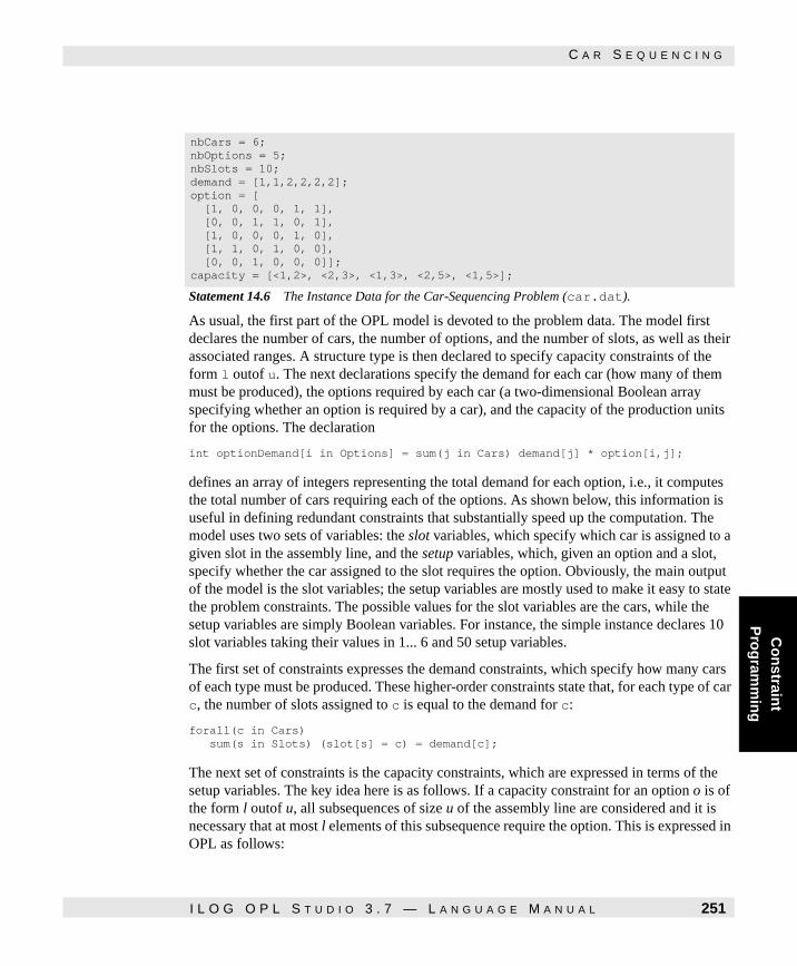
Co
nstrain
t P
rog
ramm
ing
C A R S E Q U E N C I N G
Statement 14.6
Statement 14.6 The Instance Data for the Car-Sequencing Problem (car.dat).
As usual, the first part of the OPL model is devoted to the problem data. The model first declares the number of cars, the number of options, and the number of slots, as well as their associated ranges. A structure type is then declared to specify capacity constraints of the form l outof u. The next declarations specify the demand for each car (how many of them must be produced), the options required by each car (a two-dimensional Boolean array specifying whether an option is required by a car), and the capacity of the production units for the options. The declaration
int optionDemand[i in Options] = sum(j in Cars) demand[j] * option[i,j];
defines an array of integers representing the total demand for each option, i.e., it computes the total number of cars requiring each of the options. As shown below, this information is useful in defining redundant constraints that substantially speed up the computation. The model uses two sets of variables: the slot variables, which specify which car is assigned to a given slot in the assembly line, and the setup variables, which, given an option and a slot, specify whether the car assigned to the slot requires the option. Obviously, the main output of the model is the slot variables; the setup variables are mostly used to make it easy to state the problem constraints. The possible values for the slot variables are the cars, while the setup variables are simply Boolean variables. For instance, the simple instance declares 10 slot variables taking their values in 1... 6 and 50 setup variables.
The first set of constraints expresses the demand constraints, which specify how many cars of each type must be produced. These higher-order constraints state that, for each type of car c, the number of slots assigned to c is equal to the demand for c:
forall(c in Cars) sum(s in Slots) (slot[s] = c) = demand[c];
The next set of constraints is the capacity constraints, which are expressed in terms of the setup variables. The key idea here is as follows. If a capacity constraint for an option o is of the form l outof u, all subsequences of size u of the assembly line are considered and it is necessary that at most l elements of this subsequence require the option. This is expressed in OPL as follows:
nbCars = 6; nbOptions = 5; nbSlots = 10; demand = [1,1,2,2,2,2]; option = [ [1, 0, 0, 0, 1, 1], [0, 0, 1, 1, 0, 1], [1, 0, 0, 0, 1, 0], [1, 1, 0, 1, 0, 0], [0, 0, 1, 0, 0, 0]]; capacity = [<1,2>, <2,3>, <1,3>, <2,5>, <1,5>];
I L O G O P L S T U D I O 3 . 7 — L A N G U A G E M A N U A L 251

C A R S E Q U E N C I N G
forall(o in Options & s in [1..nbSlots - capacity[o].u + 1]) sum(j in [s .. s + capacity[o].u - 1]) setup[o,j] <= capacity[o].l;
The instruction considers all options o and (almost) all slots s and makes sure that the number of cars requiring option o on the subsequence starting at s and of size capacity[o].u is not greater than the capacity capacity[o].l. For instance, option 1 (1 out of 2) generates the constraints
setup[1,1] + setup[1,2] <= 1; setup[1,2] + setup[1,3] <= 1; ...setup[1,9] + setup[1,10] <= 1;
while option 2 (2 out of 3) generates the constraints
setup[2,1] + setup[2,2] + setup[2,3] <= 2; setup[2,2] + setup[2,3] + setup[2,4] <= 2; ...setup[2,8] + setup[2,9] + setup[2,10] <= 2;
Although all constraints seem to have been enforced at this point, an important step is still missing. The setup variables and slot variables are not connected: a slot variable can be assigned a value without influencing its corresponding setup variable, and vice versa. To ensure correctness of the results, it is necessary to link the slot and setup variables. The link is easy to establish: given an option o and a slot s, setup[o,s] is 1 if the car assigned to slot s (i.e., slot[s]) requires option o (i.e., option[o,slot[s]] = 1). The resulting set of constraints is specified as follows:
forall(o in Options & s in Slots) setup[o,s] = option[o,slot[s]];
It is clear from the above instruction that the setup variables are not strictly necessary: each variable setup[o,s] could be replaced by option[o,slot[s]]. This would, however, slow down the execution of the model substantially, since constraint solving over variable-indexed arrays is expensive. It is thus best to factor out these expressions as much as possible.
All constraints have now been defined. However, the efficiency of OPL can be improved by adding redundant (or surrogate) constraints. As mentioned previously, redundant constraints do not remove any solutions: rather, they express properties of the solutions that may help OPL explore the search space more efficiently. In other words, the constraints are semantically redundant but not operationally redundant.
The car-sequencing problem has a redundant constraint worth exploiting. If option o has a capacity constraint l outof u, it follows that the last u slots can contain only l cars, so the other slots must contain all the remaining cars requiring option o, i.e.,
setup[o,1] + ...+ setup[o,nbSlots - u] >= optionDemand[o] - l.
252 I L O G O P L S T U D I O 3 . 7 — L A N G U A G E M A N U A L
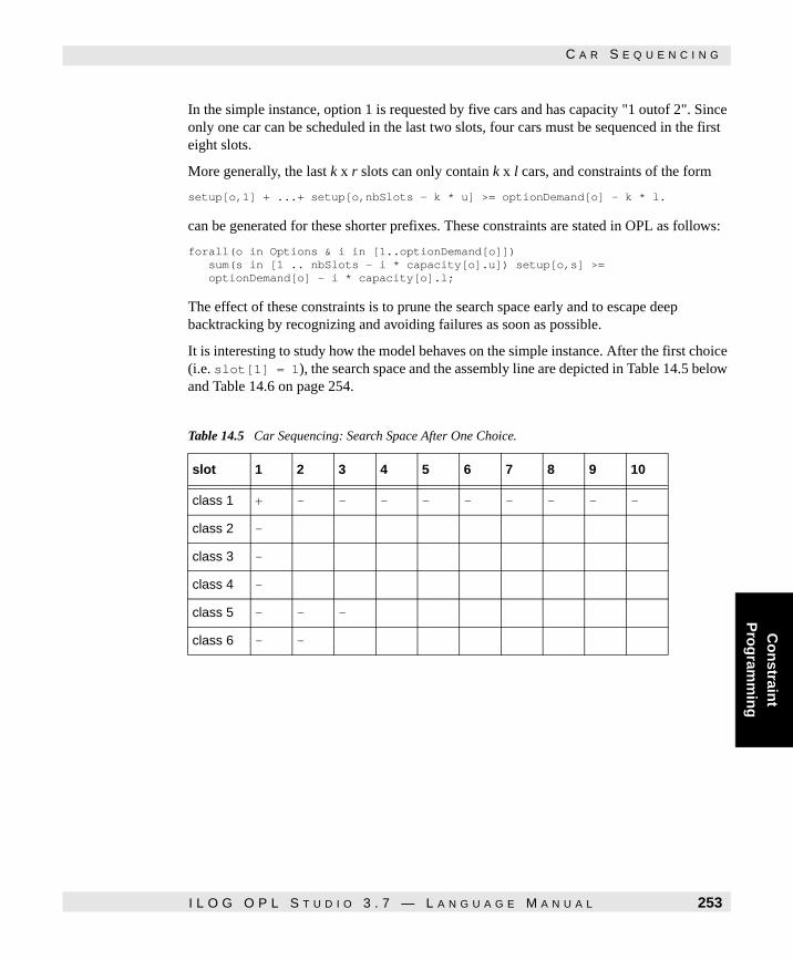
Co
nstrain
t P
rog
ramm
ing
C A R S E Q U E N C I N G
In the simple instance, option 1 is requested by five cars and has capacity "1 outof 2". Since only one car can be scheduled in the last two slots, four cars must be sequenced in the first eight slots.
More generally, the last k x r slots can only contain k x l cars, and constraints of the form
setup[o,1] + ...+ setup[o,nbSlots - k * u] >= optionDemand[o] - k * l.
can be generated for these shorter prefixes. These constraints are stated in OPL as follows:
forall(o in Options & i in [1..optionDemand[o]]) sum(s in [1 .. nbSlots - i * capacity[o].u]) setup[o,s] >= optionDemand[o] - i * capacity[o].l;
The effect of these constraints is to prune the search space early and to escape deep backtracking by recognizing and avoiding failures as soon as possible.
It is interesting to study how the model behaves on the simple instance. After the first choice (i.e. slot[1] = 1), the search space and the assembly line are depicted in Table 14.5 below and Table 14.6 on page 254.
Table 14.5 Car Sequencing: Search Space After One Choice.
slot 1 2 3 4 5 6 7 8 9 10
class 1 + - - - - - - - - -
class 2 -
class 3 -
class 4 -
class 5 - - -
class 6 - -
I L O G O P L S T U D I O 3 . 7 — L A N G U A G E M A N U A L 253

C A R S E Q U E N C I N G
Table 14.6 Car Sequencing: The Assembly Line After One Choice.
slot 1 2 3 4 5 6 7 8 9 10
option 1 + -
option 2 -
option 3 + - -
option 4 +
option 5
Table 14.7 Car Sequencing: Search Space After Two Choices (Part I).
slot 1 2 3 4 5 6 7 8 9 10
class 1 + - - - - - - - - -
class 2 - + - - - - - - - -
class 3 - -
class 4 - - - - -
class 5 - - -
class 6 - -
Table 14.8 Car Sequencing: The assembly Line After Two Choices (Part I)
slot 1 2 3 4 5 6 7 8 9 10
option 1 + -
option 2 - -
option 3 + - -
option 4 + + - - -
option 5 -
254 I L O G O P L S T U D I O 3 . 7 — L A N G U A G E M A N U A L

Co
nstrain
t P
rog
ramm
ing
C A R S E Q U E N C I N G
Table 14.9 Car Sequencing: Search Space After Two Choices (Part II).
slot 1 2 3 4 5 6 7 8 9 10
class 1 + - - - - - - - - -
class 2 - + - - - - - - - -
class 3 - -
class 4 - - - - -
class 5 - - - - - - - -
class 6 - -
Table 14.10 Car Sequencing: The assembly Line After Two Choices (Part II)
slot 1 2 3 4 5 6 7 8 9 10
option 1 + -
option 2 - - + + - + + - + +
option 3 + - -
option 4 + + - - -
option 5 -
Table 14.11 Car Sequencing: Search Space After Two Choices (Part III).
slot 1 2 3 4 5 6 7 8 9 10
class 1 + - - - - - - - - -
class 2 - + - - - - - - - -
class 3 - - - -
class 4 - - - - - -
class 5 - - - - + - - + - -
class 6 - - - -
I L O G O P L S T U D I O 3 . 7 — L A N G U A G E M A N U A L 255

T H E E U L E R T O U R
In Table 14.5 on page 253, a - sign means that a value is not in the domain of the variable and a + means that a value is assigned to the variable. In Table 14.6 on page 254, a - means that the value of the variable is 0, while + means that the value of the variable is 1. For instance, the figures show that, since classes 1 and 5 use option 3 whose capacity is 1/3, the second and third slot cannot be given a car of class 5. Now, assigning slot[2] with its first possible value, i.e. 2, leads directly to the solution presented at the beginning of the example. Indeed, this choice immediately removes the value 2 for all other slot variables and prevents variables slot[3], slot[4], and slot[5] from taking the value 4 because of option 4. This intermediate state is depicted in Tables 14.7 and 14.8. But the redundant constraints for option 2 require that slot[3] and slot[4] be assigned a class including option 2, since six cars with option 2 must be produced. The effect of these assignments is to fix all option variables concerning option 2 and to remove possible values from the slot variables. The search space at that stage is depicted in Tables 14.9 and 14.10. At this point, the demand constraints for class 5 come into play. Two cars of class 5 must be produced; since only two places are left for them, they are assigned immediately. This leads to the search space depicted in Tables 14.11 and 14.12. The final step amounts to using the redundant constraints for option 1, which fix all option variables related to option 1 and lead to the solution depicted earlier. Note that here the solution was found in two choices without any backtracking.
The Euler Tour
The Euler tour problem illustrates the global constraint circuit and membership constraints. Consider a knight on a chessboard. The problem entails moving the knight according to the rules of chess in order to visit all positions on the chessboard exactly once and return to the initial position. In more technical terms, the problem consists in finding a Hamiltonian circuit in the graph consisting of a node for each position on the chessboard and an edge for each valid knight's move. The problem of finding a Hamiltonian circuit is NP-complete.
Table 14.12 Car Sequencing: The assembly Line After Two Choices (Part III)
slot 1 2 3 4 5 6 7 8 9 10
option 1 + - - + - - +
option 2 - - + + - + + - + +
option 3 + - - + +
option 4 + + - - - -
option 5 - - -
256 I L O G O P L S T U D I O 3 . 7 — L A N G U A G E M A N U A L

Co
nstrain
t P
rog
ramm
ing
T H E E U L E R T O U R
Statement 14.7 shows an OPL model for this problem using the numbering convention in Table 14.13 on page 258 for the positions. The model associates a variable with each position in the chessboard using the array jump, where jump[i] is the location to which the knight moves from location i. An interesting feature of this model is the specification of the legal moves of the knight from each position. It uses a generic declaration that computes the values of each of its elements, where the values are sets of integers taken from the range ChessBoard. More precisely, Knightmoves[i] represents the set of legal moves from position i.
In general, for a position i, the moves are given by i-17, i-15, i-10, i-6, i+6, i+10, i+15 and i+17. For instance, the legal moves from position 37 are 20, 22, 27, 31, 47, 52 and 54.
Statement 14.7
Statement 14.7 The Euler Tour Problem (euler.mod).
range ChessBoard 1..64; {ChessBoard} Knightmove[i in ChessBoard] = { j | j in ChessBoard : i mod 8 = 1 & (j = i-15 \/ j = i-6 \/ j = i+10 \/ j = i+17) \/ i mod 8 = 2 & (j=i-17 \/ j=i-15 \/ j=i-6 \/ j=i+10 \/ j=i+15 \/ j=i+17) \/ i mod 8 >= 3 & i mod 8 <= 6 & (j=i-17 \/ j=i-15 \/ j=i-10 \/ j=i-6 \/ j=i+6 \/ j=i+10 \/ j=i+15 \/ j=i+17) \/ i mod 8 = 7 & (j=i-17 \/ j=i-15 \/ j=i-10 \/ j=i+6 \/ j=i+15 \/ j=i+17) \/ i mod 8 = 0 & (j = i-17 \/ j = i-10 \/ j = i+6 \/ j=i+15) };
var ChessBoard jump[ChessBoard];
solve { forall(p in ChessBoard) jump[p] in Knightmove[p];
circuit(jump);
forall(p in ChessBoard) sum(c in Knightmove[p]) (jump[c] = p) = 1; };
I L O G O P L S T U D I O 3 . 7 — L A N G U A G E M A N U A L 257

T H E E U L E R T O U R
A first attempt to specify knightmoves[i] is as follows:
{ChessBoard} Knightmoves[i in ChessBoard] := { j | j in ChessBoard : j = i-17 \/ j = i-15 \/ j = i-10 \/ j = i-6 \/ j = i+6 \/ j = i+10 \/ j = i+15 \/ j = i+17 };
where \/ and & denote "logical or" and "logical and" respectively. It specifies that, for a position i, the set Knightmove[i] is the set of all j in ChessBoard satisfying the equations discussed previously. However, this specification is only correct for columns 3 to 6 and it would generate invalid moves for the other columns: for instance, it would allow a move from position 25 to position 8, which is clearly invalid. It is thus necessary to generalize the above condition slightly through a case analysis, which results in the set definition shown in Statement 14.7 on page 257. It is interesting to observe the use of arbitrary Boolean combinations of conditions. There are three types of constraints in the model. The first set of constraints
forall(p in ChessBoard) jump[p] in Knightmoves[p];
are membership constraints that simply specify that variable jump[i] takes only values corresponding to legal uses. The second constraint
circuit(jump);
specifies that the set of edges
{(1,jump[1]),...,(64,jump[64])}
describes a Hamiltonian circuit or, more precisely, that the sequence
(1 , v1 ), (v1 , v2 ),..., (vn-1, vn), (vn, vn+1)
where
Table 14.13 The Numbering Used in the Euler Tour.
1 2 3 4 5 6 7 8
9 10 11 12 13 14 15 16
17 18 19 20 21 22 23 24
25 26 27 28 29 30 31 32
33 34 35 36 37 38 39 40
41 42 43 44 45 46 47 48
49 50 51 52 53 54 55 56
57 58 59 60 61 62 63 64
258 I L O G O P L S T U D I O 3 . 7 — L A N G U A G E M A N U A L

Co
nstrain
t P
rog
ramm
ing
F R E Q U E N C Y A L L O C A T I O N
is a Hamiltonian circuit. Operationally, circuit(jump) enforces the so-called subtour constraints, i.e., it makes sure that there are no subtours of length less than 64. For instance, if, at some computation stage, jump[1] = 2 and jump[2] = 3, circuit (jump) enforces the two constraints
jump[3] <> 2 & jump[3] <> 1
The last set of constraints
forall(p in ChessBoard) sum(c in Knightmoves[p]) (jump[c] = p) = 1;
are redundant constraints that make sure that each position in the board is assigned to at least one variable. These constraints are not necessary from a semantic standpoint but they help in pruning the search space.
It is interesting to see at how OPL behaves on this problem. OPL first generates values for the corners, i.e., positions 1, 8, 57, and 64 because these variables have the smallest domains. Note that the assignment
jump[1] = 11
automatically produces the assignment
jump[18] = 1
and similarly for the other corners. OPL then continues building these independent paths incrementally, connecting them only later in the computation. In essence, OPL automatically discovers the multi-path method described in Christofides [3].
Frequency Allocation
The frequency-allocation problem illustrates a number of interesting features of OPL: the use of complex quantifiers, the use of a multi-criteria ordering to choose which variable to assign next, and the functions abs and nbOccur. It also features an interesting data representation. The frequency-allocation problem consists of allocating frequencies to a number of transmitters so that there is no interference between transmitters and the number of allocated frequencies is minimized. The problem described here is an actual cellular phone problem where the network is divided into cells, each cell containing a number of transmitters whose locations are specified. The interference constraints are specified as follows:
◆ The distance between two transmitter frequencies within a cell must not be smaller than 16.
◆ The distances between two transmitter frequencies from different cells vary according to their geographical situation and are described in a matrix.
I L O G O P L S T U D I O 3 . 7 — L A N G U A G E M A N U A L 259

F R E Q U E N C Y A L L O C A T I O N
The problem of course consists of assigning frequencies to transmitters to avoid interference and, if possible, to minimize the number of frequencies. The rest of this section focuses on finding a solution using a heuristic to reduce the number of allocated frequencies.
Statement 14.8 shows an OPL statement for the frequency-allocation problem and Statement 14.9 on page 261 describes the instance data. The model data first specifies the number of cells (25 in the instance), the number of available frequencies (256 in the instance), and their associated ranges. The next declarations specify the number of transmitters needed for each cell and the distance between cells. For example, in the instance, cell 1 requires eight transmitters while cell 3 requires six transmitters. The distance between cell 1 and cell 2 is 1.
Statement 14.8
Statement 14.8 The Frequency-Allocation Problem (alloc.mod).
int nbCells = ...; int nbFreqs = ...; range Cells 1..nbCells; range Freqs 1..nbFreqs; int nbTrans[Cells] = ...; int distance[Cells,Cells] = ...;
struct TransmitterType { Cells c; int t; }; {TransmitterType} Transmitters = { <c,t> | c in Cells & t in 1..nbTrans[c] }; var Freqs freq[Transmitters];
solve { forall(c in Cells & ordered t1, t2 in 1..nbTrans[c]) abs(freq[<c,t1>] - freq[<c,t2>]) >= 16;
forall(ordered c1, c2 in Cells : distance[c1,c2] > 0) forall(t1 in 1..nbTrans[c1] & t2 in 1..nbTrans[c2]) abs(freq[<c1,t1>] - freq[<c2,t2>]) >= distance[c1,c2]; };
search { forall(t in Transmitters ordered by increasing <dsize(freq[t]),nbTrans[t.c]>) tryall(f in Freqs ordered by decreasing nbOccur(f,freq)) freq[t] = f; };
260 I L O G O P L S T U D I O 3 . 7 — L A N G U A G E M A N U A L

Co
nstrain
t P
rog
ramm
ing
F R E Q U E N C Y A L L O C A T I O N
Statement 14.9
Statement 14.9 Instance Data for the Frequency-Allocation Problem (alloc.dat).
The first interesting feature of the model is how variables are declared:
struct TransmitterType { Cells c; int t; }; {TransmitterType} Transmitters = { <c,t> | c in Cells & t in 1..nbTrans[c] }; var Freqs freq[Transmitters];
As is clear from the problem statement, transmitters are contained within cells. The above declarations preserve this structure, which will be useful when stating constraints. A transmitter is simply described as a record containing a cell number and a transmitter number inside the cell. The set of transmitters is computed automatically from the data using
{TransmitterType} Transmitters = { <c,t> | c in Cells & t in 1..nbTrans[c] };
which considers each cell and each transmitter in the cell. The model then declares an array of variables
var Freqs freq[Transmitters];
indexed by the set of transmitters; the values of these variables are of course the frequencies associated with the transmitters. There are two main groups of constraints. The first set of
nbCells = 25; nbFreqs = 256; nbTrans = [8 6 6 1 4 4 8 8 8 8 4 9 8 4 4 10 8 9 8 4 5 4 8 1 1]; distance = [ [16 1 1 0 0 0 0 0 1 1 1 1 1 2 2 1 1 0 0 0 2 2 1 1 1] [1 16 2 0 0 0 0 0 2 2 1 1 1 2 2 1 1 0 0 0 0 0 0 0 0] [1 2 16 0 0 0 0 0 2 2 1 1 1 2 2 1 1 0 0 0 0 0 0 0 0] [0 0 0 16 2 2 0 0 0 0 0 0 0 0 0 0 0 1 1 1 0 0 0 1 1] [0 0 0 2 16 2 0 0 0 0 0 0 0 0 0 0 0 1 1 1 0 0 0 1 1] [0 0 0 2 2 16 0 0 0 0 0 0 0 0 0 0 0 1 1 1 0 0 0 1 1] [0 0 0 0 0 0 16 2 0 0 1 1 1 0 0 1 1 1 1 2 0 0 0 1 1] [0 0 0 0 0 0 2 16 0 0 1 1 1 0 0 1 1 1 1 2 0 0 0 1 1] [1 2 2 0 0 0 0 0 16 2 2 2 2 2 2 1 1 1 1 1 1 1 0 1 1] [1 2 2 0 0 0 0 0 2 16 2 2 2 2 2 1 1 1 1 1 1 1 0 1 1] [1 1 1 0 0 0 1 1 2 2 16 2 2 2 2 2 2 1 1 2 1 1 0 1 1] [1 1 1 0 0 0 1 1 2 2 2 16 2 2 2 2 2 1 1 2 1 1 0 1 1] [1 1 1 0 0 0 1 1 2 2 2 2 16 2 2 2 2 1 1 2 1 1 0 1 1] [2 2 2 0 0 0 0 0 2 2 2 2 2 16 2 1 1 1 1 1 1 1 1 1 1] [2 2 2 0 0 0 0 0 2 2 2 2 2 2 16 1 1 1 1 1 1 1 1 1 1] [1 1 1 0 0 0 1 1 1 1 2 2 2 1 1 16 2 2 2 1 2 2 1 2 2] [1 1 1 0 0 0 1 1 1 1 2 2 2 1 1 2 16 2 2 1 2 2 1 2 2] [0 0 0 1 1 1 1 1 1 1 1 1 1 1 1 2 2 16 2 2 1 1 0 2 2] [0 0 0 1 1 1 1 1 1 1 1 1 1 1 1 2 2 2 16 2 1 1 0 2 2] [0 0 0 1 1 1 2 2 1 1 2 2 2 1 1 1 1 2 2 16 1 1 0 1 1] [2 0 0 0 0 0 0 0 1 1 1 1 1 1 1 2 2 1 1 1 16 2 1 2 2] [2 0 0 0 0 0 0 0 1 1 1 1 1 1 1 2 2 1 1 1 2 16 1 2 2] [1 0 0 0 0 0 0 0 0 0 0 0 0 1 1 1 1 0 0 0 1 1 16 1 1] [1 0 0 1 1 1 1 1 1 1 1 1 1 1 1 2 2 2 2 1 2 2 1 16 2] [1 0 0 1 1 1 1 1 1 1 1 1 1 1 1 2 2 2 2 1 2 2 1 2 16]]; };
I L O G O P L S T U D I O 3 . 7 — L A N G U A G E M A N U A L 261

F R E Q U E N C Y A L L O C A T I O N
constraints handles the distance constraints between transmitters inside a cell. The instruction
forall(c in Cells & ordered t1, t2 in 1..nbTrans[c]) abs(freq[<c,t1>] - freq[<c,t2>]) >= 16;
enforces the constraint that the distance between two transmitters inside a cell is at least 16. The instruction is compact mainly because we can quantify several variables in forall statements and because of the keyword ordered. Note also that the distance is computed using the function abs, which computes the absolute value of its argument (which may be an arbitrary integer expression). The second set of constraints handles the distance constraints between transmitters from different cells. The instruction
forall(ordered c1, c2 in Cells : distance[c1,c2] > 0) forall(t1 in 1..nbTrans[c1] & t2 in 1..nbTrans[c2]) abs(freq[<c1,t1>] - freq[<c2,t2>]) >= distance[c1,c2];
considers each pair of distinct cells whose distance must be greater than zero and each two transmitters in these cells, and states that the distance between the frequencies of these transmitters must be at least the distance specified in the matrix distance.
Another interesting part of this model is the search strategy. The basic structure is not surprising: OPL considers each transmitter and chooses a frequency nondeterministically. The interesting feature of the model is the heuristic. OPL chooses to generate a value for the transmitter with the smallest domain and, in case of ties, for the transmitter whose cell size is as small as possible. This multicriterion heuristic is expressed using a tuple <dsize(freq[t]),nbTrans[t.c]> to obtain
forall(t in Transmitters ordered by increasing <dsize(freq[t]),nbTrans[t.c]>)
Each transmitter is associated with a tuple < s, c >, where s is the number of its possible frequencies and c is the number of transmitters in the cell to which the transmitter belongs. A transmitter with tuple < s1 , c1 > is preferred over a transmitter with tuple < s2 , c2 > if s1 < s2 or if s1 = s2 and c1 < c2 .
Once a transmitter has been selected, OPL generates a frequency for it in a nondeterministic manner. Once again, the model specifies a heuristic for the ordering in which the frequencies must be tried. To reduce the number of frequencies, the model says to try first those values that were used most often in previous assignments.
This heuristic is implemented using a tryall instruction with the order specified using the nbOccur function (nbOccur(i,a) denotes the number of occurrences of i in array a at a given step of the execution):
forall(t in Transmitters ordered by increasing <dsize(freq[t]),nbTrans[t.c]>) tryall(f in Freqs ordered by decreasing nbOccur(f,freq)) freq[t] = f;
On the instance depicted in Statement 14.9 on page 261, OPL returns a solution with 95 frequencies.
262 I L O G O P L S T U D I O 3 . 7 — L A N G U A G E M A N U A L

Co
nstrain
t P
rog
ramm
ing
R A C K C O N F I G U R A T I O N
Rack Configuration
This problem introduces the idea of using constraints to eliminate symmetries and contains some interesting modeling issues. It also illustrates many features found in previous examples, including structures, arrays indexed by variables, and logical connectives. The problem consists of plugging a set of electronic cards into racks with electric connectors. Each card is characterized by the power it requires, while each rack model is characterized by the maximal power it can supply, its number of connectors, and its price. Each card plugged into a rack uses a connector. The purpose of the model is to find an allocation of a given set of cards into the available racks. Tables 14.14 and 14.15 specify an instance for this problem.
Statement 14.10 on page 264 shows an OPL statement for the rack-configuration problem and Statement 14.11 on page 265 shows the instance display. The model first defines the number of rack models, the number of cards, the number of racks available, and the ranges based on these constants. The model then defines two structure types to describe the properties of rack models and of cards. These types are then used to define the rack models and the cards. Note the dummy rack model that is free but has no power and no connectors (see the instance data in Statement 14.11). The inclusion of this dummy rack model makes the OPL statement simpler to write, as will become clear later on. The next declarations compute automatically the maximum number of connectors, maximum price, and maximum cost. The generic declarations build three arrays to contain the data about the powers, the connectors, and the price of each rack model.
Table 14.14 Rack Specifications.
Rack Model Power Connectors Price
1 150 8 150
2 200 16 200
Table 14.15 Card Specifications.
Card Type Power Demand
1 20 10
2 40 4
3 50 2
4 75 1
I L O G O P L S T U D I O 3 . 7 — L A N G U A G E M A N U A L 263

R A C K C O N F I G U R A T I O N
The main idea underlying the OPL statement is to consider all the racks and assign a rack model to them. Not all the racks may be needed in an optimal solution, which is why the dummy rack model is important; The assignment of a rack to the dummy model simply indicates that the rack is not needed. The OPL statement contains two main variables: the array racks, which specifies the model assigned to each available rack, and the array counters, which specifies how many cards of a given type are assigned to a given rack. In addition, a cost variable specifies the cost of a configuration.
There are three primary sets of constraints in the OPL statement. The first two sets handle the capacity constraints of the racks, and the third makes sure that all the cards are produced. The constraints
forall(r in Racks) sum(c in Cards) counters[r,c] * car[c].power <= powerData[rack[r]];
ensure that the total power of the cards assigned to a given rack does not exceed the power of the rack. Note that rack[r] is a variable and is used to index an array. The constraints
forall(r in Racks) sum(c in Cards) counters[r,c] <= connData[rack[r]];
ensure that the number of cards assigned to a given rack does not exceed the number of connectors of the rack.
Statement 14.10
Statement 14.10 The Rack-Configuration Problem (config.mod).
int nbModel = ...; int nbCard = ...; int nbRack = ...; range Models 0..nbModel-1; range Cards 0..nbCard-1; range Racks 0..nbRack-1; range RacksButFirst 1..nbRack-1; struct modelType { int power; int connectors; int price; }; struct cardType { int power; int quantity; }; modelType model[Models] = ...; cardType car[Cards] = ...;
int maxConn = max(r in Models) model[r].connectors; int maxPrice = max(r in Models) model[r].price; int maxCost = nbCard * maxPrice; int powerData[i in Models] = model[i].power; int connData[i in Models] = model[i].connectors; int priceData[i in Models] = model[i].price; var Models rack[Racks]; var int counters[Racks,Cards] in 0..nbCard; var int cost in 0..maxCost;
minimize cost subject to { forall(r in Racks) sum(c in Cards) counters[r,c] * car[c].power <= powerData[rack[r]]; forall(r in Racks) sum(c in Cards) counters[r,c] <= connData[rack[r]]; forall(c in Cards) sum(r in Racks) counters[r,c] = car[c].quantity; cost = sum(r in Racks) priceData[rack[r]]; };
264 I L O G O P L S T U D I O 3 . 7 — L A N G U A G E M A N U A L

Co
nstrain
t P
rog
ramm
ing
R A C K C O N F I G U R A T I O N
Statement 14.11
Statement 14.11 Instance Data for the Rack-Configuration Problem (config.dat).
The constraints
forall(c in Cards) sum(r in Racks) counters[r,c] = car[c].quantity;
guarantee that the right number of each type of card is produced. The last constraint
cost = sum(r in Racks) priceData[rack[r]];
simply defines the cost as the sum of the prices of all racks.
The statement described so far is a correct specification of the problem, but unfortunately contains many symmetries; in particular, any permutation of the array rack is also a solution. To remove these symmetries, it is possible to state a constraint forcing an ordering on this array. The constraints
forall(r in RacksButFirst) rack[r-1] >= rack[r];
impose a decreasing ordering on the array, removing a large number of symmetries. Other symmetries remain, however, when the same model is chosen several times. Two racks of the same model are equivalent as far as the statement is concerned and a permutation of their card assignments also leads to a new solution. As a consequence, whenever two racks are of the same model, it is appropriate to state that one of them has at least as many cards as the other:
forall(r in RacksButFirst) rack[r-1] = rack[r] => counters[r-1,0] >= counters[r,0];
Note, however, that the added constraints do not remove all the symmetries. The remaining symmetries are harder to preclude in a static way, but could be removed using a more involved search strategy.
nbModel = 3; nbCard = 4; nbRack = 5; model = [ <0, 0, 0>, <150, 8, 150>, <200, 16, 200>]; car = [ <20, 10>, <40, 4>, <50, 2>, <75, 1>];
I L O G O P L S T U D I O 3 . 7 — L A N G U A G E M A N U A L 265
N O T E S A N D R E F E R E N C E S
Notes and References
The first constraint-programming solution for the warehouse-location problem appeared in [31], [36] and featured the element constraint to index an array with variables. The first model described in this chapter is based on a refinement of that solution described in [28]. The car-sequencing model is based on [7]. The problem was motivated by an article in AI Expert [21] reporting the failure of an expert system to solve the problem and concluding that fifth-generation tools were not appropriate for the problem. The frequency-allocation problem is taken from [28]. The data-modeling facilities of OPL avoid the tedious encoding that plagues the program described there. The rack-configuration problem is also borrowed from [28] and the model is based on the constraint program described there.
266 I L O G O P L S T U D I O 3 . 7 — L A N G U A G E M A N U A L

C H A P T E R
Sch
edu
ling
15
Scheduling
This chapter applies OPL to some scheduling and resource-allocation applications. It is generally organized around the various types of resources (e.g., unary and discrete resources and reservoirs). Elements of Chapter 4, Data Modeling and Chapter 5, Expressions and Constraints are reprinted in various places throughout to make the presentation more self-contained.
Origin and Horizon
All scheduling concepts used in OPL are defined over a global time interval
[scheduleOrigin,scheduleHorizon)
closed on the left and open on the right, like all time intervals in OPL. OPL has default values for both the origin (0) and the horizon (a large number). However, it is recommended that they be specified for particular applications, since smaller time intervals make OPL more space- and time-efficient. The global origin and horizon can be specified by using instructions of the form
scheduleOrigin = 0; scheduleHorizon = 364;
I L O G O P L S T U D I O 3 . 7 — L A N G U A G E M A N U A L 267

A C T I V I T I E S
and these instructions must be defined before the definition of any other scheduling concepts. This is consistent with our convention of requiring that each object be used only after it has been defined.
Activities
The most fundamental concept in OPL for scheduling applications is probably the activity. An activity can be thought of as an object containing three data items, a starting date, a duration, and an ending date, together with the duration constraint stating that the ending date is the starting date plus the duration. In many applications, the duration of an activity is known and the activity is declared together with its duration, as in
Activity carpentry(10);
which declares an activity carpentry whose duration is 10. The starting and ending dates of carpentry are integer variables taking their values in the global time interval and consistent with the duration constraints. Activities can also be given a variable duration, in which case the task is usually declared with an integer variable representing the duration, as in
var int durationCarpentry in 8..10; Activity carpentry(durationCarpentry);
which declares an activity carpentry whose duration is between 8 and 10. The duration variable durationCarpentry can appear in the problem constraints and the possible values for duration can thus be further constrained. It is also possible to declare an activity without specifying its duration, as in
Activity carpentry;
in which case the duration is an integer variable ranging over the interval
[0; scheduleHorizon - scheduleOrigin]
Arrays of activities can be declared in the usual way and the durations can be specified as described previously. For instance, it is traditional to declare an array of activities as follows:
Activity tasks[t in 1..10](duration[t]);
The statement declares an array of 10 activities whose activities are duration[1],...,duration[10]. Some activities may be breakable: they can start before a break and be resumed after a break. Activities in OPL are assumed to be unbreakable unless specified otherwise. The declaration
Activity a breakable;
specifies that a is a breakable activity. Of course, breakable activities behave very much like other activities: they have a starting date, an ending date, and a duration, and they may
268 I L O G O P L S T U D I O 3 . 7 — L A N G U A G E M A N U A L
Sch
edu
ling
U N A R Y R E S O U R C E S
require resources like activities. Their only added functionality is the ability to be interrupted by breaks. It is of course possible to declare arrays of breakable activities. For instance, the declaration
Activity tasks[t in 1..10](duration[t]) breakable;
defines an array of 10 breakable activities. Finally, it may be useful to declare an array that has both standard and breakable activities. This makes easy to produce generic models that are parametrized by the status of each activity. The declaration
Activity tasks[t in 1..10](duration[t]) breakable if t in breakableSet;
defines an array of 10 activities, some of which can be breakable. Practical applications may also involve transition times between activities. To simplify the modeling of these applications, OPL makes it possible to associate a transition type with each activity. The declaration
Activity tasks[t in 1..10](duration[t]) transitionType trType[t]
associates transition type trType[t] to activity t. This transition type is used by unary or state resources to make sure that the appropriate transition times (as specified when declaring the resource) are respected.
The starting date, the duration, and the ending date of an activity are accessed as the fields of a structure. For instance, a precedence constraint between two activities a and b can be specified as follows:
b.start >= a.end;
or, alternatively,
b.start >= a.start + a.duration;
In fact, OPL also has a specific constraint for expressing precedence constraints, which is recommended since it produces better visualizations of the results. For instance, a precedence constraint between two activities a and b can be specified as follows:
a precedes b;
Unary Resources
A unary resource is one that cannot be shared by two activities; i.e., as soon as an activity requires a resource, for a time interval, no other activity can use it during the same time interval. Unary resources can be used to model a variety of applications. A typical example of a unary resource is a machine in a job-shop scheduling application. This section reviews scheduling applications involving unary resources.
I L O G O P L S T U D I O 3 . 7 — L A N G U A G E M A N U A L 269

U N A R Y R E S O U R C E S
Summary of the Concepts
Unary resources are declared in OPL simply as
UnaryResource crane;
As usual, it is possible to declare arrays of unary resources, as in
UnaryResource machines[1..10];
which declares an array of 10 machines.
Once unary resources are declared, it is possible to specify which activities require them. To specify in OPL that an activity excavation requires a resource crane during its execution, it is sufficient to write the constraint
excavation requires crane;
At any time in the computation, OPL makes sure that no two activities requiring the same unary resource are scheduled at the same time. OPL also uses these constraints to update the starting and ending dates of the activities. Recall as well that unary resources can have transition times associated with them.
The Bridge Problem
The bridge problem involves of finding a schedule that minimizes the time needed to build a five-segment bridge. The project contains a set of 46 tasks and a set of constraints among these tasks (see Table 15.1 on page 275). Besides the usual precedence constraints, the problem also contains some resource constraints. Most tasks require a resource (e.g., a crane) and tasks requiring the same resource cannot overlap in time. In addition, the following additional constraints must be satisfied:
1. The time between the completion of a particular formwork and the completion of its corresponding concrete foundation is at most 4 days.
2. There are at most 3 days between the end of a particular excavation (or foundation piles) and the beginning of the corresponding formwork.
3. The formworks must start at least 6 days after the beginning of the erection of the temporary housing.
4. The removal of the temporary housing can start two days before the end of the last masonry work.
5. The delivery of the preformed bearers occurs at least 30 days after the beginning of the project.
Statements 15.1, 15.2, and 15.3 describe an OPL model for the bridge problem.
270 I L O G O P L S T U D I O 3 . 7 — L A N G U A G E M A N U A L

Sch
edu
ling
U N A R Y R E S O U R C E S
Statement 15.1
Statement 15.1 The Bridge Problem (Part I) (bridge.mod).
Statement 15.1 depicts the data used in the bridge problem. The enumerated type declarations define the set of tasks and the set of resources. The type declarations define two record types to express distance and precedence constraints. The next declarations specify an array duration for the durations of the tasks, various sets of distance constraints, an array res which associates each resource with a set of tasks using the resource, and the set of precedence constraints. Note that most of this data is initialized offline (see Statement 15.3 on page 273).
enum Task ...; enum Resource ...; struct Distance { Task before; Task after; int dist; }; struct Precedence { Task before; Task after; }; struct Disjunction { Task first; Task second; }; int duration[Task] = ...; {Distance} max nf = ...; {Distance} min sf = ...; {Distance} min ef = ...; {Distance} min nf = ...; {Distance} min af = ...; {Task} res[Resource] = ...; {Precedence} precedences = ...; int maxDuration = sum(t in Task) duration[t];
I L O G O P L S T U D I O 3 . 7 — L A N G U A G E M A N U A L 271

U N A R Y R E S O U R C E S
Statement 15.2
Statement 15.2 The Bridge Problem (Part II) (bridge.mod).
scheduleHorizon = maxDuration;
Activity a[t in Task](duration[t]);
UnaryResource tool[Resource];
minimize a[stop].start subject to { forall(t in precedences) a[t.before] precedes a[t.after];
forall(t in max nf) a[t.before].end + t.dist >= a[t.after].start;
forall(t in max ef) a[t.before].end + t.dist >= a[t.after].end;
forall(t in min af) a[t.before].start + t.dist <= a[t.after].start;
forall(t in min sf) a[t.before].start + t.dist >= a[t.after].end;
forall(t in min nf) a[t.before].end + t.dist <= a[t.after].start;
forall(r in Resource) forall(t in res[r]) a[t] requires tool[r] };
272 I L O G O P L S T U D I O 3 . 7 — L A N G U A G E M A N U A L

Sch
edu
ling
U N A R Y R E S O U R C E S
Statement 15.3
Statement 15.3 The Bridge Problem (Part III) (bridge.dat).
Statement 15.2 on page 272 is the core of the model. The declaration
scheduleHorizon = maxDuration;
defines the schedule horizon as the summation of all durations, which is certainly an upper bound to the project duration. The declaration
Activity a[t in Task](duration[t]);
defines the activities. There is one activity for each enumerated value in Task and its duration is duration[t]. Recall that an activity is composed of three items: a starting date, a duration, and an ending date, with the constraint that the ending date is equal to the starting date plus the duration.
Task = { start a1 a2 a3 a4 a5 a6 p1 p2 ue s1 s2 s3 s4 s5 s6 b1 b2 b3 b4 b5 b6 ab1 ab2 ab3 ab4 ab5 ab6 m1 m2 m3 m4 m5 m6 l t1 t2 t3 t4 t5 ua v1 v2 k1 k2 stop}; Resource = {excavator piledriver carpentry concretemizer bricklaying crane caterpillar}; duration = #[ first:0 a1:4 a2:2 a3:2 a4:2 a5:2 a6:5 p1:20 p2:13 ue:10 s1:8 s2:4 s3:4 s4:4 s5:4 s6:10 b1:1 b2:1 b3:1 b4:1 b5:1 b6:1 ab1:1 ab2:1 ab3:1 ab4:1 ab5:1 ab6:1 m1:16 m2:8 m3:8 m4:8 m5:8 m6:20 l:2 t1:12 t2:12 t3:12 t4:12 t5:12 ua:10 v1:15 v2:10 k1:0 k2:0 last:0]#; max nf = { <first l 30> <a1 s1 3> <a2 s2 3> <a5 s5 3> <a6 s6 3> <p1 s3 3> <p2 s4 3> }; min sf = { <ua m1 2> <ua m2 2> <ua m3 2> <ua m4 2> <ua m5 2> <ua m6 2> }; max ef = { <s1 b1 4> <s2 b2 4> <s3 b3 4> <s4 b4 4> <s5 b5 4> <s6 b6 4> }; min nf = { <first l 30> }; min af = { <ue s1 6> <ue s2 6> <ue s3 6> <ue s4 6> <ue s5 6> <ue s6 6> }; res = #[ crane : {t1 t2 t3 t4 t5} bricklaying : {m1 m2 m3 m4 m5 m6} carpentry : {s1 s2 s3 s4 s5 s6} excavator : {a1 a2 a3 a4 a5 a6} piledriver : {p1 p2} concretemixer : {b1 b2 b3 b4 b5 b6} caterpillar : {v1 v2}]#; precedences = { <first a1> <first a2> <first a3> <first a4> <first a5> <first a6> <first ue> <a1 s1> <a2 s2> <a5 s5> <a6 s6> <a3 p1> <a4 p2> <p1 s3> <p2 s4> <p1 k1> <p2 k1> <s1 b1> <s2 b2> <s3 b3> <s4 b4> <s5 b5> <s6 b6> <b1 ab1> <b2 ab2> <b3 ab3> <b4 ab4> <b5 ab5> <b6 ab6> <ab1 m1> <ab2 m2> <ab3 m3> <ab4 m4> <ab5 m5> <ab6 m6> <m1 t1> <m2 t1> <m2 t2> <m3 t2> <m3 t3> <m4 t3> <m4 t4> <m5 t4> <m5 t5> <m6 t5> <m1 k2> <m2 k2> <m3 k2> <m4 k2> <m5 k2> <m6 k2> <l t1> <l t2> <l t3> <l t4> <l t5> <t1 v1> <t5 v2> <t2 last> <t3 last> <t4 last> <v1 last> <v2 last> <ua last> <k1 last> <k2 last> }; };
I L O G O P L S T U D I O 3 . 7 — L A N G U A G E M A N U A L 273

U N A R Y R E S O U R C E S
The instruction
UnaryResource tool[Resource];
declares the unary resources. There is one unary resource for each enumerated value in Resource. The rest of Statement 15.2 on page 272 describes the constraints and the objective function. The objective function simply states that the starting date of the last task must be minimized. The constraint
forall(t in precedences) a[t.before] precedes a[t.after];
states the precedence constraints. An equivalent formulation, as far as the model is concerned, is
forall(<before,after> in precedences) a[before].start + a[before].duration <= a[after].start;
The first formulation is recommended, however, since it produces better visualizations of the results. The distance constraints are similar in nature to precedence constraints and should cause little difficulty. The constraint
forall(r in Resource) forall(t in res[r]) a[t] requires tool[r]
specifies the resource constraints in a concise way. It considers each resource r and each task t requiring the resource and states that activity a[t] requires unary resource tool[r] during its execution. Since the resource is unary, this constraint implies that no other task requiring tool[r] can overlap in time with a[t]. The optimal solution produced by OPL for the bridge problem is
Optimal Solution with Objective Value: 104
a[start] = [0 -- 0 --> 0] a[a1] = [4 -- 4 --> 8] a[a2] = [2 -- 2 --> 4] a[a3] = [8 -- 2 --> 10] a[a4] = [0 -- 2 --> 2] a[a5] = [13 -- 2 --> 15] a[a6] = [35 -- 5 --> 40] ...
Each activity is displayed by giving its starting date, its duration, and its ending date. For instance,
a[a5] = [13 -- 2 --> 15]
reports that activity a[a5] starts at day 13, lasts two days, and ends at day 15.
It is interesting to study the computational model for this problem. Since only unary resources are involved, the default search procedure first ranks all unary resources, i.e., determines, for each resource, a total ordering for all activities requiring the resource.
274 I L O G O P L S T U D I O 3 . 7 — L A N G U A G E M A N U A L

Sch
edu
ling
U N A R Y R E S O U R C E S
Once they are all are ranked, it is easy to find a solution, since the remaining problem is essentially a PERT problem. As a consequence, the search space explored (implicitly) by OPL on this bridge problem is the set of all possible rankings of all unary resources.
Table 15.1 Data for the Bridge Problem.
N Name Description Duration Resource
1 PA beginning of project 0 -
2 A1 excavation (abutment 1) 4 excavator
3 A2 excavation (pillar 1) 2 excavator
4 A3 excavation (pillar 2) 2 excavator
5 A4 excavation (pillar 3) 2 excavator
6 A5 excavation (pillar 4) 2 excavator
7 A6 excavation (pillar 5) 5 excavator
8 P1 foundation piles 2 20 pile-driver
9 P2 foundation piles 3 13 pile-driver
10 UE erection of temporary housing 10 -
11 S1 formwork (abutment 1) 8 carpentry
12 S2 formwork (pillar 1) 4 carpentry
13 S3 formwork (pillar 2) 4 carpentry
14 S4 formwork (pillar 3) 4 carpentry
15 S5 formwork (pillar 4) 4 carpentry
16 S6 formwork (abutment 2) 10 carpentry
17 B1 concrete foundation (abutment 1) 1 concrete-mixer
18 B2 concrete foundation (pillar 1) 1 concrete-mixer
19 B3 concrete foundation (pillar 2) 1 concrete-mixer
20 B4 concrete foundation (pillar 3) 1 concrete-mixer
21 B5 concrete foundation (pillar 4) 1 concrete-mixer
22 B6 concrete foundation (abutment 2) 1 concrete-mixer
I L O G O P L S T U D I O 3 . 7 — L A N G U A G E M A N U A L 275

U N A R Y R E S O U R C E S
23 AB1 concrete setting time (abutment 1) 1 -
24 AB2 concrete setting time (pillar 1) 1 -
25 AB3 concrete setting time (pillar 2) 1 -
26 AB4 concrete setting time (pillar 3) 1 -
27 AB5 concrete setting time (pillar 4) 1 -
28 AB6 concrete setting time (abutment 2) 1 -
29 M1 masonry work (abutment 1) 16 bricklaying
30 M2 masonry work pillar 1) 8 bricklaying
31 M3 masonry work (pillar 2) 8 bricklaying
32 M4 masonry work (pillar 3) 8 bricklaying
33 M5 masonry work (pillar 4) 8 bricklaying
34 M6 masonry work (abutment 2) 20 bricklaying
35 L delivery of preformed bearers 2 crane
36 T1 positioning (preformed bearer 1) 12 crane
37 T2 positioning (preformed bearer 2) 12 crane
38 T3 positioning (preformed bearer 3) 12 crane
39 T4 positioning (preformed bearer 4) 12 crane
40 T5 positioning (preformed bearer 5) 12 crane
41 UA removal of temporary housing 10 -
42 V1 filling 1 15 caterpillar
43 V2 filling 2 10 caterpillar
44 K1 cost point 1 0 -
45 K2 cost point 2 0 -
46 PE end of project 0 -
Table 15.1 Data for the Bridge Problem. (Continued)
N Name Description Duration Resource
276 I L O G O P L S T U D I O 3 . 7 — L A N G U A G E M A N U A L
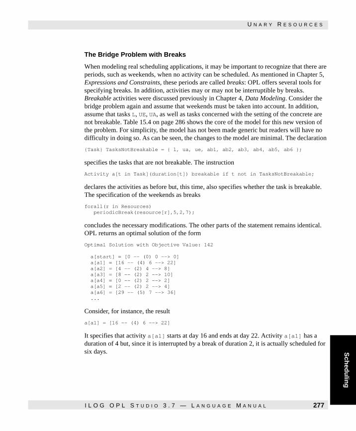
Sch
edu
ling
U N A R Y R E S O U R C E S
The Bridge Problem with Breaks
When modeling real scheduling applications, it may be important to recognize that there are periods, such as weekends, when no activity can be scheduled. As mentioned in Chapter 5, Expressions and Constraints, these periods are called breaks: OPL offers several tools for specifying breaks. In addition, activities may or may not be interruptible by breaks. Breakable activities were discussed previously in Chapter 4, Data Modeling. Consider the bridge problem again and assume that weekends must be taken into account. In addition, assume that tasks L, UE, UA, as well as tasks concerned with the setting of the concrete are not breakable. Table 15.4 on page 286 shows the core of the model for this new version of the problem. For simplicity, the model has not been made generic but readers will have no difficulty in doing so. As can be seen, the changes to the model are minimal. The declaration
{Task} TasksNotBreakable = { l, ua, ue, ab1, ab2, ab3, ab4, ab5, ab6 };
specifies the tasks that are not breakable. The instruction
Activity a[t in Task](duration[t]) breakable if t not in TasksNotBreakable;
declares the activities as before but, this time, also specifies whether the task is breakable. The specification of the weekends as breaks
forall(r in Resources) periodicBreak(resource[r],5,2,7);
concludes the necessary modifications. The other parts of the statement remains identical. OPL returns an optimal solution of the form
Optimal Solution with Objective Value: 142
a[start] = [0 -- (0) 0 --> 0] a[a1] = [16 -- (4) 6 --> 22] a[a2] = [4 -- (2) 4 --> 8] a[a3] = [8 -- (2) 2 --> 10] a[a4] = [0 -- (2) 2 --> 2] a[a5] = [2 -- (2) 2 --> 4] a[a6] = [29 -- (5) 7 --> 36] ...
Consider, for instance, the result
a[a1] = [16 -- (4) 6 --> 22]
It specifies that activity a[a1] starts at day 16 and ends at day 22. Activity a[a1] has a duration of 4 but, since it is interrupted by a break of duration 2, it is actually scheduled for six days.
I L O G O P L S T U D I O 3 . 7 — L A N G U A G E M A N U A L 277

U N A R Y R E S O U R C E S
Job-Shop Scheduling
Job-shop scheduling problems can be modeled easily in OPL. Statement 15.5 on page 280 describes a simple job-shop scheduling model. The problem is to schedule a number of jobs on a set of machines to minimize completion time, often called the makespan. Each job is a sequence of tasks and each task requires a machine. Statement 15.5 first declares the number of machines, the number of jobs, and the number of tasks in the jobs. The main data of the problem, i.e., the duration of all the tasks and the resources they require, are then given. The instructions
Activity task[j in Jobs, t in Tasks](duration[j,t]); Activity makespan(0);
UnaryResource tool[Machines];
declares the activities and the unary resources. Note that the makespan is modeled for simplicity as an activity of duration zero. The first set of constraints specifies that the makespan is not smaller than the ending time of the last task of each job. The next two sets specify the precedence and disjunctive constraints.
On the instance data shown in Statement 15.6 on page 280, OPL returns an optimal solution of the form
Optimal Solution with Objective Value: 55
task[1,1] = [5 -- 1 --> 6] task[1,2] = [6 -- 3 --> 9] task[1,3] = [16 -- 6 --> 22] task[1,4] = [30 -- 7 --> 37] task[1,5] = [42 -- 3 --> 45] task[1,6] = [49 -- 6 --> 55] ...
278 I L O G O P L S T U D I O 3 . 7 — L A N G U A G E M A N U A L

Sch
edu
ling
U N A R Y R E S O U R C E S
Statement 15.4
Statement 15.4 The Bridge Problem with Breaks (Part II) (bridgebr.mod).
{Task} TasksNotBreakable = { l, ua, ue, ab1, ab2, ab3, ab4, ab5, ab6 };
scheduleHorizon = maxDuration; Activity a[t in Task](duration[t]) breakable if t not in TasksNotBreakable;
UnaryResource tool[Resource];
minimize a[stop].start subject to { forall(r in Resource) periodicBreak(tool[r],5,2,7);
forall(t in precedences) a[t.before] precedes a[t.after];
forall(t in max nf) a[t.before].end + t.dist >= a[t.after].start;
forall(t in max ef) a[t.before].end + t.dist >= a[t.after].end;
forall(t in min af) a[t.before].start + t.dist <= a[t.after].start;
forall(t in min sf) a[t.before].start + t.dist >= a[t.after].end;
forall(t in min nf) a[t.before].end + t.dist <= a[t.after].start;
forall(r in Resource) forall(t in res[r]) a[t] requires tool[r] };
I L O G O P L S T U D I O 3 . 7 — L A N G U A G E M A N U A L 279

U N A R Y R E S O U R C E S
Statement 15.5
Statement 15.5 A Job-Shop Scheduling Model (jobshop.mod).
Statement 15.6
Statement 15.6 Data for the Job-Shop Scheduling Model (jobshop.dat).
int nbMachines = ...; range Machines 1..nbMachines; int nbJobs = ...; range Jobs 1..nbJobs; int nbTasks = ...; range Tasks 1..nbTasks;
Machines resource[Jobs,Tasks] = ...; int+ duration[Jobs,Tasks] = ...; int totalDuration = sum(j in Jobs, t in Tasks) duration[j,t];
ScheduleHorizon = totalDuration; Activity task[j in Jobs, t in Tasks](duration[j,t]); Activity makespan(0);
UnaryResource tool[Machines];
minimize makespan.end subject to { forall(j in Jobs) task[j,nbTasks] precedes makespan;
forall(j in Jobs) forall(t in 1..nbTasks-1) task[j,t] precedes task[j,t+1];
forall(j in Jobs) forall(t in Tasks) task[j,t] requires tool[resource[j,t]]; };
nbMachines = 6; nbJobs = 6; nbTasks = 6;
resource = [ [3 1 2 4 6 5] [2 3 5 6 1 4] [3 4 6 1 2 5] [2 1 3 4 5 6] [3 2 5 6 1 4] [2 4 6 1 5 3]]; duration = [ [1 3 6 7 3 6] [8 5 10 10 10 4] [5 4 8 9 1 7] [5 5 5 3 8 9] [9 3 5 4 3 1] [3 3 9 10 4 1]];
280 I L O G O P L S T U D I O 3 . 7 — L A N G U A G E M A N U A L

Sch
edu
ling
U N A R Y R E S O U R C E S
Search Procedures
In scheduling applications with unary resources, the general strategy is to rank each unary resource. Ranking a unary resource consists of finding a total ordering for all activities requiring the resource. Once activities are ordered, a solution can be found efficiently. The constructs and procedures available for search procedures were discussed in Chapter 7, Search. This section reviews some of the tools available to rank unary resources.
The highest-level tool available in OPL to assist the ranking process is a nondeterministic instruction rank that ranks all unary resources in the schedule. This instruction is implemented in terms of simpler instructions of the form
rank(u)
where rank(u) ranks all activities using unary resource u.
Choosing which resource to rank next may be important in some applications. OPL supports this process through a number of reflective functions depicted in Table 15.2 on page 281. The global slack of a resource considers all activities that are not yet ranked, computes the earliest starting date s, the latest finishing date e, and the total duration d of all these activities, and returns (e - s) - d. This produces an approximation of the tightness of the resource at a given computation point. The local slack of a unary resource, another measure of tightness that is more precise but more expensive to compute, entails computing the global slack for a variety of subsets of the unranked activities.
Table 15.2 Reflective Functions on Unary resources.
Function Type Semantics
isRanked(Unary) int 1 if the resource is ranked and 0 otherwise
isRanked([Unary]) int 1 if all resources are ranked and 0 otherwise
nbPossibleFirst(Unary) int number of activities which can be ranked first
nbPossibleLast(Unary) int number of activities which can be ranked last
isPossibleFirst(Unary r,Activity a) int true if a can potentially be ranked first on r
isPossibleLast(Unary,Activity) int true if a can potentially be ranked last on r
localSlack(Unary) int local slack of the resource
globalSlack(Unary) int global slack of the resource
I L O G O P L S T U D I O 3 . 7 — L A N G U A G E M A N U A L 281

U N A R Y R E S O U R C E S
Using these functions, it is possible to define search strategies such as
forall(r in Resources ordered by increasing localSlack(tool[r])) rank(u[r]);
It is interesting to consider how to rank a resource. Ranking a resource u could be handled as follows:
while not isRanked(u) do select(t in Tasks : not isRanked(u,a[t])) tryRankFirst(u,a[t]);
assuming that array a indexed by elements of Tasks contains all the activities requiring resource u. The condition isRanked(u) returns true if and only if resource u is ranked. It can also be applied to an array of unary resources, in which case it returns true whenever all resources are ranked. The condition
isRanked(u,a)
returns true whenever activity a is already ranked on unary resource u. The instruction
tryRankFirst(u,a)
is nondeterministic and has two alternatives. The first alternative adds the constraint that a be ranked first among the unranked activities of u. The second alternative (used on backtracking) adds the constraint specifying that a cannot rank first among the unranked activities of u. OPL also provides a nondeterministic instruction tryRankLast that tries to rank an activity last among the unranked activities of a resource.
Once again, it may be important to choose which activity to rank next. OPL supports this process in a variety of ways. First, it is possible to use the starting dates of each activity and predefined functions available on variables. For instance, the heuristic that ranks next the variable with the earliest starting date can be expressed as
select(t in Tasks : not isRanked(u,a[t]) ordered by increasing dmin(a[t].start)) tryRankFirst(u,a[t]);
In addition to that support, OPL provides also two other predefined functions. The function
isPossibleFirst(u,a)
holds if activity a can potentially be ranked first on resource u. Function
isPossibleLast(u,a)
holds if activity a can potentially be ranked last on resource u at this computation stage. Although in the above discussion a resource is ranked completely before considering the next resource, other strategies are of course possible.
282 I L O G O P L S T U D I O 3 . 7 — L A N G U A G E M A N U A L

Sch
edu
ling
D I S C R E T E R E S O U R C E S
For instance, the excerpt
while not isRanked(tool) do select(r in Resources : not isRanked(tool[r])) select(t in tasks[r] : not isRanked(tool[r],a[t]) tryRankFirst(tool[r],a[t]);
selects a resource and an activity and tries to rank first the activity on the resource. It then selects a resource again (which may be different from the resource first selected if heuristics are used for the selection) and an activity.
Search Strategies
In job-shop scheduling applications, it is often beneficial to use a search strategy based on discrepancy search, e.g., slice-based search or depth-bounded discrepancy search. These strategies exploit the fact that the heuristics used in scheduling applications are often of good quality and hence they may produce high-quality solutions faster than depth-first search. The excerpt
search { SBSsearch() { rankLocal; } };
illustrates the use of such a strategy for job-shop scheduling.
Discrete Resources
A discrete resource is a resource with a discrete capacity. The capacity, which may vary over time, represents the number of available copies (or instances) of the resource. For instance, a discrete resource may be used to model a budget, as in Chapter 2, A Short Tour of OPL, a set of "equivalent" workers, or a set of similar machines. This section presents several applications of discrete resources that complement the problem described in the section Scheduling on page 64.
Summary of the Concepts
A discrete resource is a resource whose capacity is a strictly positive integer. Discrete resources are declared in OPL by specifying their capacity, as in
DiscreteResource crane(3);
which specifies that crane is a resource of capacity 3, i.e., there are three cranes available. It is possible to declare arrays of discrete resources, as in
DiscreteResource res[t in 1..10](cap[t]);
I L O G O P L S T U D I O 3 . 7 — L A N G U A G E M A N U A L 283

D I S C R E T E R E S O U R C E S
which declares an array of 10 resources, the capacity of resource i being cap[i]. While a unary resource is a discrete resource of capacity 1, the algorithms for unary resources are optimized to exploit all properties of this special case.
Activities can require discrete resources in the same way as unary resources. In addition, an activity can require a certain capacity of the discrete resource. For instance, the constraint
a requires(2) crane;
specifies that activity a requires two cranes. The capacity requested can be an arbitrary integer expression, possibly containing variables. The underlying algorithms in OPL ensure that the amount requested at any time does not exceed the capacity of the resource. In fact, three levels of pruning can be achieved in OPL for discrete resources: the default level, the disjunctive level, and the edge-finder level. The disjunctive level can be requested by declarations of the form
DiscreteResource crane(3) using disjunctive;
This level of pruning makes sure that, if the total demand of a set of activities requires more than the capacity of the resource, at least one of these activities is scheduled before another activity in the set. The edge-finder level can be requested by declarations of the form
DiscreteResource crane(3) using edgeFinder;
This edge-finder level generalizes the edge-finding algorithm of unary resources to discrete resources. It tries to deduce which activities must be scheduled first (or last) in a set whose total demand exceeds the capacity of the resource. Which level of propagation is appropriate depends, of course, on the application at hand.
As mentioned previously, a constraint
a requires(2) r
specifies that activity a requires 2 units of the resource r during its execution. As a consequence, as soon as activity a terminates, its requested capacity is returned to the resource r and is available for other activities. For some applications (e.g., when the discrete resource denotes a budget), the requested capacity should not be returned to the resource: it is consumed. This functionality is obtained in OPL by stating constraints of the form
a consumes(2) r;
Note that it is also possible to use consumes for unary resources, although in general this is not particularly useful. The capacity of a discrete resource may also vary over time, generalizing the concept of breaks in unary resources. The capacity of a discrete resource over time can be specified with constraints of the form
capacityMax(<DiscreteResource>,<Start>,<End>,<Cap>) capacityMin(<DiscreteResource>,<Start>,<End>,<Cap>)
A constraint capacityMax(d,s,e,c) specifies that the capacity of discrete resource d required by activities over the interval [s,e) is at most c, while a constraint
284 I L O G O P L S T U D I O 3 . 7 — L A N G U A G E M A N U A L

Sch
edu
ling
D I S C R E T E R E S O U R C E S
capacityMin(d,s,e,c) specifies that the capacity of discrete resource d required by activities over the interval [s,e) is at least c.
Note that this last constraint in fact constrains the scheduling of activities.
The Ship-Loading Problem
This application schedules the loading of a ship. It consists of 34 activities subject to precedence constraints, as depicted in Table 15.3. In addition, all of these activities have durations and require a unique resource of capacity 8 in various quantities, as depicted in Table 15.4 on page 286. For instance, activity 1 has a duration of 3 and requests 4 units of the discrete resource. The goal of the application is to minimize the makespan (i.e., the time to load the ship) while satisfying the precedence and capacity constraints. Statement 15.7 on page 287 gives an OPL model for solving this problem. It is interesting to review some of the new functionalities of OPL used in this model. First, the declaration
DiscreteResource res(8);
declares a discrete resource of capacity 8. Second, the constraint
forall(t in Tasks) a[t] requires(demand[t]) res;
specifies that activity a[t] requires demand[t] units of the discrete resource.
Table 15.3 Precedence Constraints for the Ship-Loading Problem.
Activity Successors Activity Successors Activity Successors Activity Successors
1 2 4 11 13 21 22 31 28
2 3 12 13 22 23 32 33
3 5 7 13 15 16 23 24 33 34
4 5 14 15 24 25 34
5 6 15 18 25 26 30 31 32
6 8 16 17 26 27
7 8 17 18 27 28
8 9 18 19 20 21 28 29
9 10 14 19 19 29
10 11 12 20 20 30 28
I L O G O P L S T U D I O 3 . 7 — L A N G U A G E M A N U A L 285

D I S C R E T E R E S O U R C E S
For this application, OPL returns an optimal solution of the form
Optimal Solution with Objective Value: 66
a[1] = [0 -- 3 --> 3] a[2] = [3 -- 4 --> 7] a[3] = [7 -- 4 --> 11] a[4] = [3 -- 6 --> 9] ...
Table 15.4 Capacity Constraints for the Ship-Loading Problem.
Act. Dur. Cap. Act. Dur. Cap. Act. Dur. Cap. Act. Dur. Cap.
1 3 4 11 3 4 21 1 4 31 2 3
2 4 4 12 2 5 22 2 4 32 1 3
3 4 3 13 1 4 23 4 7 33 2 3
4 6 4 14 5 3 24 5 8 34 2 3
5 5 5 15 2 3 25 2 8
6 2 5 16 3 3 26 1 3
7 3 4 17 2 6 27 1 3
8 4 3 18 2 7 28 2 6
9 3 4 19 1 4 29 1 8
10 2 8 20 1 4 30 3 3
286 I L O G O P L S T U D I O 3 . 7 — L A N G U A G E M A N U A L

Sch
edu
ling
D I S C R E T E R E S O U R C E S
Statement 15.7
Statement 15.7 The Ship-Loading Problem (shipload.mod).
Observe that, at time 3, activities a[2] and a[4] both require 4 units of the resource, implying that no other activity can be scheduled at this time. The efficiency of the model can be improved by using the choice specification
search { setTimes };
since the application involves only precedence and resource constraints. It is important to stress here that the solution assigns to an activity the resource necessary at any given time during its execution. However, the resource may be different at two given times, since the resources are considered "equivalent". The section From Discrete to Unary Resources on page 288 discusses how to transform discrete resources into a set of unary resources for some applications.
int capacity = 8; int nbTasks = 34; range Tasks 1..nbTasks; int duration[Tasks] = [ 3, 4, 4, 6, 5, 2, 3, 4, 3, 2, 3, 2, 1, 5, 2, 3, 2, 2, 1, 1, 1, 2, 4, 5, 2, 1, 1, 2, 1, 3, 2, 1, 2, 2]; int totalDuration = sum(t in Tasks) duration[t]; int demand[Tasks] = [ 4, 4, 3, 4, 5, 5, 4, 3, 4, 8, 4, 5, 4, 3, 3, 3, 6, 7, 4, 4, 4, 4, 7, 8, 8, 3, 3, 6, 8, 3, 3, 3, 3, 3]; struct Precedences { int before; int after; }; {Precedences} setOfPrecedences = { <1, 2>, <1, 4>, <2, 3>, <3, 5>, <3, 7>, <4, 5>, <5, 6>, <6, 8>, <7, 8>, <8, 9>, <9, 10>, <9, 14>, <10, 11>, <10, 12>, <11, 13>, <12, 13>, <13, 15>, <13, 16>, <14, 15>, <15, 18>, <16, 17>, <17, 18>, <18, 19>, <18, 20>, <18, 21>, <19, 23>, <20, 23>, <21, 22>, <22, 23>, <23, 24>, <24, 25>, <25, 26>, <25, 30>, <25, 31>, <25, 32>, <26, 27>, <27, 28>, <28, 29>, <30, 28>, <31, 28>, <32, 33>, <33, 34> };
scheduleHorizon = totalDuration; Activity a[t in Tasks](duration[t]); DiscreteResource res(8); Activity makespan(0); minimize makespan.end subject to { forall(t in Tasks) a[t] precedes makespan; forall(p in setOfPrecedences) a[p.before] precedes a[p.after]; forall(t in Tasks) a[t] requires(demand[t]) res; };
I L O G O P L S T U D I O 3 . 7 — L A N G U A G E M A N U A L 287

D I S C R E T E R E S O U R C E S
The Perfect Square Problem Revisited
This second application of discrete resources reconsiders the perfect square problem described in the section Search Procedures on page 61.
Statement 15.8 on page 289 gives a model for this problem using discrete resources. The key insight is to represent a square by two activities x[i] and y[i] whose durations are the size of the square. Of course, the starting dates of x[i] and y[i] represent the coordinates of the bottom-left corner of the square. The master square is approximated by two discrete resources rx and ry whose capacities are the size of the master square. The activities x[i] require discrete resource rx while the activities y[i] require ry, both equal in capacity to the square they represent (or, as a matter of fact, to their duration): i.e.,
forall(s in Squares) { x[s] requires(size[s]) rx; y[s] requires(size[s]) ry };
In addition, the model imposes capacity constraints on the discrete resources to ensure that there is no empty space, i.e.,
capacityMin(rx,0,SizeSquare,SizeSquare); capacityMin(ry,0,SizeSquare,SizeSquare);
Of course, these constraints are only approximations and do not capture the two-dimensionality of the application. They are best viewed as redundant or surrogate constraints. The only "real" constraints are the non-overlapping constraints, i.e.,
forall(ordered i, j in Squares) x[i].end <= x[j].start \/ x[j].end <= x[i].start \/ y[i].end <= y[j].start \/ y[j].end <= y[i].start;
From Discrete to Unary Resources
For applications using a collection of unary resources that are considered "equivalent", it is often of benefit to use a discrete resource and then convert the solution of the discrete resource problem into a solution to the original problem. This methodology avoids the exploration of a set of highly symmetrical configurations and thus may significantly reduce the search space. For instance, a job shop may have three machines with identical functionalities and the application may not care which of them is actually used for performing a given task. Discrete resources are particularly attractive in this case because, as soon as a solution to the discrete resource problem has been found, it can easily be converted into an actual solution to the problem with unary resources. This principle can be illustrated on a variant of the house problem discussed in the section Scheduling on page 64. In this variant, the tasks are still subject to the same precedence constraints but the budget constraints are dropped. Instead, each task requires a worker. There are three workers; Thomas, Maite, and Antoine, who are considered "equivalent" for the purpose of the application. The problem is to minimize the completion date subject to these constraints.
288 I L O G O P L S T U D I O 3 . 7 — L A N G U A G E M A N U A L

Sch
edu
ling
D I S C R E T E R E S O U R C E S
Statement 15.9 on page 291 gives an OPL model for this problem in which each worker is a unary resource. In addition, the model declares a discrete resource pool of capacity 3 that aggregates the workers (Once again, the model could be made completely generic; it is specialized to the instance data only for simplicity). It also uses an array use of 0/1 variables to specify which worker is associated with the tasks. The problem constraints consist mainly of the precedence constraints and the discrete resource constraints
forall(t in Tasks) a[t] requires(1) pool;
The remaining constraints
forall(t in Tasks, w in Workers) a[t] requires(use[t,w]) worker[w];
forall(t in Tasks) sum(w in Workers) use[t,w] = 1;
are essentially inactive during the search, as will shortly become clear. They specify that each task must be assigned a unique worker.
Statement 15.8
Statement 15.8 The Perfect Square Problem Revisited (squarea.mod)
int SizeSquare = 112; int NbSquares = 21; range Squares 1..NbSquares; range Positions 1..SizeSquare;int size[Squares]=[50,42,37,35,33,29,27,25,24,19,18,17,16,15,11,9,8,7,6,4,2];
scheduleHorizon = SizeSquare; Activity x[s in Squares](size[s]); Activity y[s in Squares](size[s]); DiscreteResource rx(SizeSquare); DiscreteResource ry(SizeSquare);
solve { capacityMin(rx,0,SizeSquare,SizeSquare); capacityMin(ry,0,SizeSquare,SizeSquare); forall(ordered i, j in Squares) x[i].end <= x[j].start \/ x[j].end <= x[i].start \/ y[i].end <= y[j].start \/ y[j].end <= y[i].start; forall(s in Squares) { x[s] requires(size[s]) rx; y[s] requires(size[s]) ry }; }; search { setTimes(x); setTimes(y); };
I L O G O P L S T U D I O 3 . 7 — L A N G U A G E M A N U A L 289

D I S C R E T E R E S O U R C E S
Note that the constraints
forall(t in Tasks, w in Workers) a[t] requires(use[t,w]) worker[w];
require capacity zero or one, depending on the value of the variables in use. This functionality is discussed again later in this chapter. The search procedure here is most interesting. The instruction setTimes(a); actually solves the problem: it assigns a starting date to each activity so that the discrete resource constraints are satisfied. When this instruction succeeds, the existence of a solution is guaranteed. The remaining part of the search procedure
once { forall(t in Tasks ordered by increasing dmin(a[t].start)) tryall(w in Workers) use[t,w] = 1; }
simply converts the solution of the discrete resource problem into a solution to the original problem. It considers all tasks in the order given by their starting dates and assigns to them the first worker available by assigning the appropriate element of use to one. Since the discrete capacity constraints are satisfied, a worker must be available at this date. Note that the instruction
forall(t in Tasks ordered by increasing dmin(a[t].start)) tryall(w in Workers) use[t,w] = 1;
is enclosed in a once instruction, since only one such solution is required.
Search Procedures
This section reviews the search support provided by OPL for scheduling applications involving discrete resources. In scheduling applications with discrete resources, two activities that require the same resource may overlap in time. However, the total capacity required by the activities at any given time t may not exceed the capacity available at time t. As a consequence, a solution to these scheduling problems must assign specific times to the activities, producing a computational model fundamentally different from unary resources.
OPL also provides an instruction setTimes(a) that assigns starting dates to all activities in an array a. This instruction should not be applied blindly: in some situations it can miss solutions (e.g., when there are negative distance constraints of the form a.start >= b.end - 3). However, for problems with discrete resources, positive distance constraints, and activities with fixed duration, it may improve efficiency considerably over a more naive
290 I L O G O P L S T U D I O 3 . 7 — L A N G U A G E M A N U A L

Sch
edu
ling
D I S C R E T E R E S O U R C E S
strategy. Of course, it is often possible to make choices to come into a position where setTimes can be applied naturally.
Statement 15.9
Statement 15.9 Converting Discrete to Unary Resources (house1.mod).
Under this hypothesis, the basic idea behind setTimes can be explained as follows. If d is the earliest date at which an activity can start, OPL selects a task that can be scheduled at date d. On backtracking, another task is selected to start at d, or execution fails if none are available. Tasks that are not scheduled at their earliest date are said to be postponed, and remain so until their starting dates are updated. Because of the nature of the problem and because of the properties of constraint propagation in OPL, one of these activities must start at date d in an optimal solution. Once such a task is chosen, OPL considers the next date n >= d at which a non-postponed activity can start and also all the tasks that can start at n. Once again, one of these tasks is chosen nondeterministically to start at date n. Note that
enum Tasks {masonry,carpentry,plumbing,ceiling,roofing,painting,windows,facade,garden,moving};int duration[Tasks] = [7,3,8,3,1,2,1,2,1,1]; enum Workers { Thomas, Maite, Antoine };
scheduleHorizon = sum(t in Tasks) duration[t]; DiscreteResource pool(3); Activity a[t in Tasks](duration[t]); UnaryResource worker[Workers]; var int use[Tasks,Workers] in 0..1;
minimize a[moving].end subject to { a[masonry] precedes a[carpentry]; a[masonry] precedes a[plumbing]; a[masonry] precedes a[ceiling]; a[carpentry] precedes a[roofing]; a[ceiling] precedes a[painting]; a[roofing] precedes a[windows]; a[roofing] precedes a[facade]; a[plumbing] precedes a[facade]; a[roofing] precedes a[garden]; a[plumbing] precedes a[garden]; a[windows] precedes a[moving]; a[facade] precedes a[moving]; a[garden] precedes a[moving]; a[painting] precedes a[moving];
forall(t in Tasks) a[t] requires(1) pool;
forall(t in Tasks, w in Workers) a[t] requires(use[t,w]) worker[w];
forall(t in Tasks) sum(w in Workers) use[t,w] = 1; }; search { setTimes(a); once { forall(t in Tasks ordered by increasing dmin(a[t].start)) tryall(w in Workers) use[t,w] = 1; } };
I L O G O P L S T U D I O 3 . 7 — L A N G U A G E M A N U A L 291

R E S E R V O I R S
some tasks may have a minimal starting date smaller than n. These are of course the postponed activities, because there exists an optimal solution in which these tasks do not take a value in the range d+1..n. If the current partial solution can be extended to an optimal solution, the starting dates of these tasks have to be updated, enabling OPL to reconsider them. Moreover, if the latest starting date of one of the postponed activities is smaller than n, then this postponed activity cannot have its starting date updated, meaning that the current partial solution cannot be extended to an optimal solution. This process is iterated until all the tasks have been assigned a starting date (a solution has been found) or only postponed activities remain (failure). Finally, since it may be important in some applications to choose which resources and activities should be considered next, OPL offers, for discrete resources, generalizations of the functions localSlack and globalSlack, presented earlier for unary resources. As mentioned previously, these functions give an approximate measure of the tightness of a resource.
Reservoirs
Unary and discrete resources are appropriate modeling tools when activities only require (or consume) resources. Some applications, however, may have a combination of activities, some requiring resources and others providing resources. For instance, an activity may require a resource plumber, while the plumber Joe may provide the resource plumber. Resources that can be required and provided are called reservoirs in OPL.
Summary of the Concepts
A reservoir is declared as in
Reservoir plumbing(3);
which declares a reservoir plumbing of maximum capacity 3 and initial capacity 0. The capacity of the reservoir specifies the difference between the supply (i.e., what is provided or produced) and the demand (what is required or consumed). A second parameter can be added to specify the initial capacity as in
Reservoir plumbing(3,1);
As usual, it is also possible in OPL to declare arrays of reservoirs. Activities can require reservoirs in the same way as they require discrete resources:
a requires(2) plumbing;
specifies that activity a requires two units of plumbing during its execution. Activities can also consume the reservoir, as in
a consumes(2) plumbing;
292 I L O G O P L S T U D I O 3 . 7 — L A N G U A G E M A N U A L

Sch
edu
ling
R E S E R V O I R S
In addition to these constraints, activities can also provide and produce reservoirs. The constraint
b provides(2) plumbing;
specifies that activity b provides two units of plumbing during its execution, while the constraint
b produces(2) plumbing;
specifies that activity b produces two units of plumbing from its end date to the horizon. Of course, providing and producing are the counterparts to requiring and consuming.
The House Problem with Reservoirs
We now illustrate reservoirs on an application that brings up many modeling issues. The problem consists, once again, of building a house and the activities are the same as previously described. However, this time, the starting dates of these activities are known and the issue is to allocate a "worker" to each of them. Each of the activities can be performed by a group of workers. In addition, each group of workers has a maximum capacity, so that only a subset of its workers can be allocated at any given time. Table 15.5 on page 293 gives some of the instance data for this problem: the name of each task, its duration, its starting date, and the groups that can perform the task. There are three groups, g1, g2 and g3. Group g1 has three workers, Thomas, Brett, and Matthew, and has a capacity of 2. Group g2 has one worker, Scott, and group g3 has also one worker, Bill. The goal of the application is to allocate workers to tasks while minimizing the time spent by a worker on the construction site.
Table 15.5 Instance Data for the House Problem with Workers.
Name Duration Start Groups
masonry 7 0 {g1, g2}
carpentry 3 7 {g1, g3}
plumbing 8 7 {g2}
ceiling 3 7 {g1, g3}
roofing 1 10 {g1, g3}
painting 2 10 {g2, g3}
windows 1 11 {g1, g3}
facade 2 15 {g1, g2}
garden 1 15 {g1, g2, g3}
moving 1 17 {g1, g3}
I L O G O P L S T U D I O 3 . 7 — L A N G U A G E M A N U A L 293

R E S E R V O I R S
The model for this application, given in Statement 15.10 on page 295, is non-trivial and involves a number of previously seen concepts. The first set of declarations consists primarily of associating an activity with each task. Of course, the duration and the starting date of each activity are well known: the duration is specified during the activity declaration, while the starting date is enforced by the constraint
forall(t in Tasks) task[t].start = start[t];
The second set of declarations concerns the groups of workers. The key idea in this model is to associate a reservoir with each group. The activities require units from these reservoirs, while the workers provide units for these reservoirs. In addition to the reservoirs, the model uses a two-dimensional array perform of Boolean variables to keep track of which group perform each activities. More precisely, perform[g,t] is 1 if group g performs activity t and 0 otherwise. Several constraints are expressed in terms of these data. The constraint
forall(t in Tasks) sum(g in mayperform[t]) perform[g,t] = 1;
specifies that each task must be performed by exactly one group. The constraint
forall(t in Tasks) forall(g in mayperform[t]) task[t] requires(perform[g,t]) group[g];
specifies that a task t requires a group g if and only if g performs t. This is expressed concisely by using variable perform[g,t] as the capacity required. When g does not perform t, there is no requirement constraint. When g performs t, there is a requirement constraint of capacity 1. The last set of declarations concerns the workers. Each worker is an activity whose duration is unknown, i.e., it is a variable ranging over 0..totalDuration. These activities provide units for the groups in the constraint
forall(g in Groups) forall(w in workers[g]) worker[w] provides group[g];
294 I L O G O P L S T U D I O 3 . 7 — L A N G U A G E M A N U A L

Sch
edu
ling
R E S E R V O I R S
Statement 15.10
Statement 15.10 Allocating Workers for the House Problem (house4.mod).
The model is now complete. The remaining instructions are included only to improve efficiency. The constraint
forall(g in Groups) forall(ordered v, w in workers[g]) worker[w].start >= worker[v].start & worker[w].end >= worker[v].end;
removes symmetries between the workers to avoid exploring "equivalent" solutions, since workers are identical resources in this model.
enum Tasks {masonry,carpentry,plumbing,ceiling,roofing,painting,windows,facade,garden,moving};int duration[Tasks] = [7,3,8,3,1,2,1,2,1,1]; int totalDuration = sum(t in Tasks) duration[t]; scheduleHorizon = totalDuration; int start[Tasks] = [0,7,7,7,10,10,11,15,15,17]; Activity task[t in Tasks](duration[t]);
enum Groups { g1, g2, g3 }; int capacity[Groups] = [2, 1, 1]; {Groups} mayperform[Tasks] = #[ masonry:{g1,g2}, carpentry:{g1,g3}, plumbing:{g2}, ceiling:{g1,g3}, roofing:{g1,g3}, painting:{g2,g3}, windows:{g1,g3}, facade:{g1,g2}, garden:{g1,g2,g3}, moving:{g1,g3}]#; var int perform[Groups,Tasks] in 0..1; Reservoir group[g in Groups](capacity[g]);
enum Workers { Thomas, Brett, Matthew, Scott, Bill }; {Workers} workers[Groups] = #[g1:{ Thomas, Brett, Matthew }, g2:{ Scott }, g3:{Bill}]#; var int durationWorkers[Workers] in 0..totalDuration; Activity worker[t in Workers](durationWorkers[t]);
minimize max(w in Workers) durationWorkers[w] subject to { forall(t in Tasks) task[t].start = start[t]; /* starts of Tasks */ forall(t in Tasks) /* resource constraints */ forall(g in mayperform[t]) task[t] requires(perform[g,t]) group[g]; forall(t in Tasks) sum(g in mayperform[t]) perform[g,t] = 1; /* one resource must be used */ forall(g in Groups) /* providing the resources */ forall(w in workers[g]) worker[w] provides group[g]; forall(g in Groups) /* removing Symmetries */ forall(ordered v, w in workers[g]) worker[w].start >= worker[v].start & worker[w].end >= worker[v].end; }; search { forall(t in Workers) { generate(durationWorkers[t]); generate(worker[t].start); }; generate(perform); };
I L O G O P L S T U D I O 3 . 7 — L A N G U A G E M A N U A L 295

S T A T E R E S O U R C E S
The choice specification
search { forall(t in Workers) { generate(durationWorkers[t]); generate(worker[t].start); }; };
simply defines the order of enumeration for the variables: considers the various workers and assigns a duration and a starting date to each of them in sequence.
State Resources
Some applications require the use of state resources, i.e., resources that are specified by a set of states and of activities requiring that a resource be in some state to be of interest. This section reviews an application of this type.
Summary of the Concepts
State resources are resources that are specified by a set of possible states. A state resource is declared as follows:
enum States { hot, warm, cold }; StateResource oven(States);
These instructions declare an oven that can take three states: hot, warm, and cold. The constraint
a requiresState(warm) oven;
where a is an activity, expresses that the oven must be warm during the execution of a. It is also possible to specify that a state resource must be in a set of states during the execution of an activity as in
enum States { hot, warm, cold }; StateResource oven(States); {States} notCold = { hot, warm }; Activity a(10); solve { a requiresAnyState(notCold) oven; }
that a state resource must not be in a state, e.g.
a excludesState(cold) oven;
or in a set of states
a excludesAllStates(notCold) oven;
during the execution of an activity.
296 I L O G O P L S T U D I O 3 . 7 — L A N G U A G E M A N U A L

Sch
edu
ling
S T A T E R E S O U R C E S
The Trolley Problem
To illustrate state resources, consider the following problem. A number of jobs must be performed in a shop equipped with a number of machines. Each job corresponds to the processing of an item that needs to be sequentially processed on a number of machines for some known duration. Each item is initially available in area A of the shop. It must be brought to the specified machines with a trolley. After it has been processed on all machines, it must be stored in area S of the shop. Moving an item from area x to area y consists of (1) loading the item on the trolley at area x; (2) moving the trolley from area x to area y and (3) unloading the item from the trolley at area y. The goal is to find a schedule minimizing the makespan. In this version of the problem, we ignore the time to move the trolley and we assume that loading and unloading activities at some area can overlap and that the trolley has unlimited capacity. We will show how to lift some of these restrictions in the next section.
The specific instance considered here consists of 6 jobs, each of which requires processing on two specified machines. As a consequence, a job consists of 8 tasks
1. load the item on the trolley at area A;
2. unload the item from the trolley at the area of the first machine required by the job;
3. process the item on the first machine;
4. load the item on the trolley at the area of this machine;
5. unload the item from the trolley at the area of the second machine required by the job;
6. process the item on the second machine;
7. load the item on the trolley at the area of this machine;
8. unload the item from the trolley at Area S;
Statements 15.11 and 15.12 depict an OPL model for this problem. The statement starts by defining the set of jobs, the set of tasks to be performed by the jobs, and the states of the trolley. The tasks correspond to the description given previously. The trolley has five states, one for each available machine, one for the arrival area, and one for the storage area. The statement then defines the data for the jobs, i.e., it specifies the two machines required for each job and the duration of the activities to be performed on these machines. The machines are specified by a number (in 1..3) and the instruction
States state[1..3] = [m1,m2,m3];
is used to map such a number into a state for the trolley. The next two declarations specify the load (and unload) duration and the schedule horizon. The next instruction
StateResource trolley(States);
defines the trolley as a set of resources with five possible states. The instructions
UnaryResource machine[1..3]; Activity act[Jobs,Tasks];
I L O G O P L S T U D I O 3 . 7 — L A N G U A G E M A N U A L 297

D I S C R E T E E N E R G Y R E S O U R C E S
define the unary resources (for the machines) and the activities for all the tasks of the jobs. The constraint part of the statement specifies the duration, the precedence, the unary resource, and the state resource constraints. Of particular interest are the state resource constraints
forall(j in Jobs) { act[j,loadA] requiresState(areaa) trolley; act[j,unload1] requiresState(state[job[j].machine1]) trolley; act[j,load1] requiresState(state[job[j].machine1]) trolley; act[j,unload2] requiresState(state[job[j].machine2]) trolley; act[j,load2] requiresState(state[job[j].machine2]) trolley; act[j,unloadS] requiresState(areaS) trolley; };
that specify the state of the trolley for each of the loading and unloading tasks. For instance, the constraint
act[j,loadA] requiresState(areaA) trolley;
specifies that task loadA of activity j requires the trolley to be in state areaA.
Discrete Energy Resources
It is often important in practical applications to obtain schedules with varying granularities over time. Typically, one is interested in a precise schedule in the short-term and coarser schedules in the medium- and long-terms. For instance, one may be interested in a daily schedule for the first six months, a weekly schedule for the next six months, and a monthly schedule for the next year. Discrete energy resources make it possible to specify the time steps to be considered by OPL over some time intervals and are a fundamental tool for these applications.
Summary of the Concepts
Discrete energy resources can be thought of as a generalization of discrete resource that enables users to specify time steps over the schedule horizon. A discrete energy resource is declared by specifying its capacity and by specifying the time steps for the various successive time intervals that constitute the relevant scheduling period. Consider for instance a problem where two workers must be assigned to some tasks and assume that we are interested in a schedule whose time steps are a day for the first week (a week is considered to consist of five days), two days for the next two weeks, and a week for the remaining of the schedule.
A discrete energy resource of the form
int step[1..2] = [1,2,5]; int time[1..5] = [scheduleOrigin,5,15,scheduleHorizon]; DiscreteEnergy workers(2,step,time);
298 I L O G O P L S T U D I O 3 . 7 — L A N G U A G E M A N U A L

Sch
edu
ling
D I S C R E T E E N E R G Y R E S O U R C E S
can be used for that purpose. It specifies that workers is a discrete energy resource of capacity two, with a time step of 1 for the interval [scheduleOrigin,5), a time step of 2 for the interval [5,15), and a time step of 5 days for the rest of the schedule. It is also interesting to consider what would be a legal schedule for the second and third week. Here the time step is 2 days and of course there are two workers available for each day. Hence, for every two successive days, the total "energy" available is 4 workers and, as a consequence, any solution can only schedule, over these two days, activities whose total capacity demand does not exceed 4. Note that only the total demand over the two days is constrained; for instance, there may be three activities (of duration one) requesting a worker on day 5 and one activity requesting a worker on day 6. More generally, on the above example, the total energy is 2 for each interval [t,t+1) in [0,5), 4 for each interval [t,t+2) in [5,15), and 10 for each interval [t,t+5) in the rest of the schedule and the activities scheduled in these intervals must satisfy the appropriate energy constraints.
Statement 15.11
Statement 15.11 The Trolley Problem: Part I (state.mod).
enum Jobs {j1,j2,j3,j4,j5,j6}; enum Tasks {loadA,unload1,process1,load1,unload2,process2,load2,unloadS}; enum States {m1,m2,m3,areaA,areaS}; struct jobRecord { int machine1; int durations1; int machine2; int durations2; }; jobRecord job[Jobs] = [ <1,80,2,60>, <2,120,3,80>, <2,80,1,60>, <1,160,3,100>, <3,180,2,80>, <2,140,3,60> ]; States state[1..3] = [m1,m2,m3]; int loadDuration = 20; scheduleHorizon = card(Jobs) * card(Tasks) * loadDuration + sum(j in Jobs) (job[j].durations1 + job[j].durations2); StateResource trolley(States); UnaryResource machine[1..3]; Activity act[Jobs,Tasks]; Activity makespan(0);
I L O G O P L S T U D I O 3 . 7 — L A N G U A G E M A N U A L 299

D I S C R E T E E N E R G Y R E S O U R C E S
Statement 15.12
Statement 15.12 The Trolley Problem: Part II (state.mod).
Activities can require/consume discrete energy resources in the same way as discrete resources. The underlying algorithms in OPL make sure that the total energy of the resource at the various time intervals is not exceeded. The energy of a discrete energy resource over time can be specified with methods whose signatures are
setEnergyMin(<Start>,<End>,<Energy>) setEnergyMax(<Start>,<End>,<Energy>)
For instance, if d is a discrete energy resource, then the method
d.setEnergyMin(1,5,2)
specifies that the energy of d over time interval [1,5) is no less than 2, while the method
d.setEnergyMax(1,5,5)
specifies that the energy of d over time interval [1,5) is no more than 5. There are also various reflective methods over discrete energy resources to access the energy of a discrete energy resource at various times or time intervals. These are described in Chapter 5, Expressions and Constraints.
minimize makespan.end subject to { forall(j in Jobs) { act[j,loadA].duration = loadDuration; act[j,unload1].duration = loadDuration; act[j,process1].duration = job[j].durations1; act[j,load1].duration = loadDuration; act[j,unload2].duration = loadDuration; act[j,process2].duration = job[j].durations2; act[j,load2].duration = loadDuration; act[j,unloadS].duration = loadDuration; }; forall(j in Jobs) forall(ordered t1, t2 in Tasks) act[j,t1] precedes act[j,t2]; forall(j in Jobs) { act[j,process1] requires machine[job[j].machine1]; act[j,process2] requires machine[job[j].machine2]; }; forall(j in Jobs) { act[j,loadA] requiresState(areaA) trolley; act[j,unload1] requiresState(state[job[j].machine1]) trolley; act[j,load1] requiresState(state[job[j].machine1]) trolley; act[j,unload2] requiresState(state[job[j].machine2]) trolley; act[j,load2] requiresState(state[job[j].machine2]) trolley; act[j,unloadS] requiresState(areaS) trolley; }; forall(j in Jobs) act[j,unloadS] precedes makespan; };
300 I L O G O P L S T U D I O 3 . 7 — L A N G U A G E M A N U A L
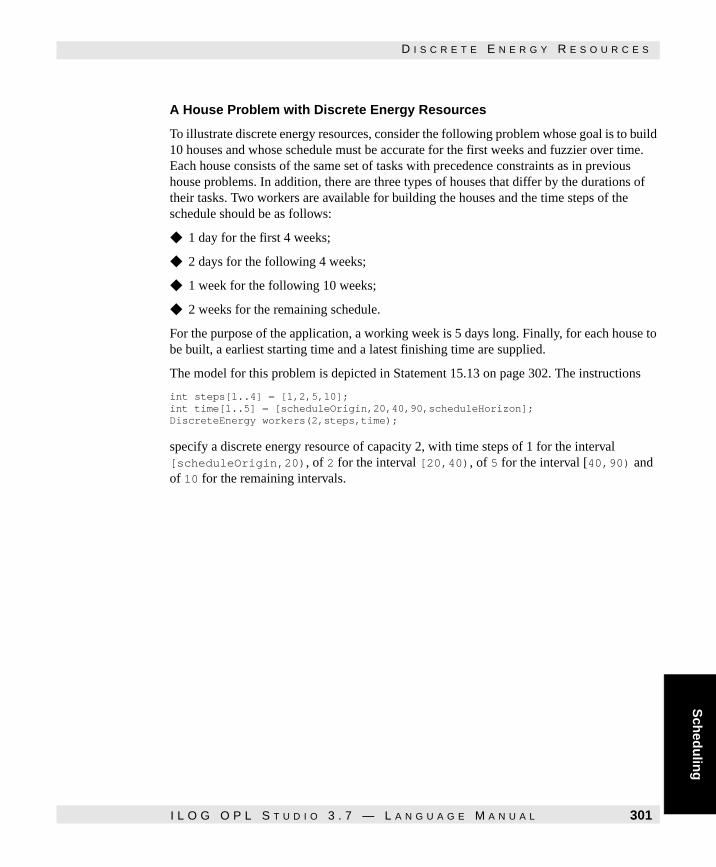
Sch
edu
ling
D I S C R E T E E N E R G Y R E S O U R C E S
A House Problem with Discrete Energy Resources
To illustrate discrete energy resources, consider the following problem whose goal is to build 10 houses and whose schedule must be accurate for the first weeks and fuzzier over time. Each house consists of the same set of tasks with precedence constraints as in previous house problems. In addition, there are three types of houses that differ by the durations of their tasks. Two workers are available for building the houses and the time steps of the schedule should be as follows:
◆ 1 day for the first 4 weeks;
◆ 2 days for the following 4 weeks;
◆ 1 week for the following 10 weeks;
◆ 2 weeks for the remaining schedule.
For the purpose of the application, a working week is 5 days long. Finally, for each house to be built, a earliest starting time and a latest finishing time are supplied.
The model for this problem is depicted in Statement 15.13 on page 302. The instructions
int steps[1..4] = [1,2,5,10]; int time[1..5] = [scheduleOrigin,20,40,90,scheduleHorizon]; DiscreteEnergy workers(2,steps,time);
specify a discrete energy resource of capacity 2, with time steps of 1 for the interval [scheduleOrigin,20), of 2 for the interval [20,40), of 5 for the interval [40,90) and of 10 for the remaining intervals.
I L O G O P L S T U D I O 3 . 7 — L A N G U A G E M A N U A L 301

D I S C R E T E E N E R G Y R E S O U R C E S
Statement 15.13
Statement 15.13 A House Problem with a Discrete Energy Resource (energy.mod)
The rest of the statement should not raise any difficulty. The model produces a solution of the form
Solution [1]
act[1,masonry] = [128 -- 7 --> 135] ... act[1,moving] = [192 -- 1 --> 193] act[2,masonry] = [120 -- 7 --> 127] ... act[2,moving] = [192 -- 1 --> 193] ... act[10,masonry] = [107 -- 15 --> 122] ... act[10,moving] = [190 -- 1 --> 191]
makespan = [193 -- 0 --> 193]
enum Tasks { masonry, carpentry, plumbing, ceiling, roofing, painting, windows, facade, garden, moving }; range TypeHouse 1..3; int duration[TypeHouse,Tasks] = [ [7,3,8,3,1,2,1,2,1,1] , [12,5,10,5,2,5,2,3,2,1] , [15,3,10,6,2,3,2,3,2,1]]; setof(Tasks) precedences[Tasks] = #[ masonry:{carpentry,plumbing,ceiling},carpentry:{roofing},ceiling:{painting}, roofing:{windows,facade,garden},plumbing:{facade,garden},windows:{moving}, facade:{moving},garden:{moving},painting:{moving}, moving:{} ]#; scheduleHorizon = 200; struct House { int typeHouse; int startMin; int endMax; }; range RHOUSE 1..10; House houses[RHOUSE] = [ <1,0,200>, <1,20,200>, <1,0,150>, <1,100,200>, <2,0,150>, <2,10,150>, <2,100,200>, <2,0,150>, <3,30,100>, <3,90,200> ]; int steps[1..4] = [1,2,5,10]; int time[1..5] = [scheduleOrigin,20,40,90,scheduleHorizon]; DiscreteEnergy workers(2,steps,time); Activity act[RHOUSE,Tasks]; Activity makespan(0); solve { forall(h in RHOUSE & t in Tasks) { act[h,t].duration = duration[houses[h].typeHouse,t]; act[h,t] requires workers; }; forall(h in RHOUSE & t in Tasks & o in precedences[t]) act[h,t] precedes act[h,o]; forall(h in RHOUSE) { act[h,moving] precedes makespan; act[h,masonry].start >= houses[h].startMin; act[h,moving].end <= houses[h].endMax; }; }; search setTimes;
302 I L O G O P L S T U D I O 3 . 7 — L A N G U A G E M A N U A L

Sch
edu
ling
T R A N S I T I O N T I M E S
Transition Times
Practical applications often involve transition times between activities, in order to, say, set up new tools. This section shows how to use transition times in OPL.
Summary of the Main Concepts
Transition times can be specified between any two activities requiring the same unary and state resource. Given two activities a and b, the transition time between a and b is the amount of time that must elapse between the end of a and the beginning of b when a precedes b. Typically, transition times depend on the nature of the activities. If activities a and b use, say, the same tools, the transition time may be small or nonexistent. If they use fundamentally different tools, the transition times may be larger.
Transition times are specified in two steps in OPL. First, every activity involving transition times must be associated with a transition type (an integer or an enumerated value). Second, the unary or state resource must be associated with a transition matrix that, given two transition types, returns a transition time.
The Trolley Example Revisited
Consider again the trolley problem presented earlier and assume that the time to move the trolley from an area to another must be taken account. This new requirement can be taken into account by using transition times. The key idea is that each activity may be associated with a transition type that represents the location where the activity is taking place. For instance, task unload1 of job j1 is associated with state m1 if the first machine of j1 is machine 1. The state resource can be associated with a transition matrix that, given two locations, return the time to move from one to the other. Statement 15.14 on page 304 and Statement 15.15 depict the OPL model for this problem. The declaration
int m[States,States] = [ [ 0, 50, 60, 50, 90 ], [ 50, 0, 60, 90, 50 ], [ 60, 60, 0, 80, 80 ], [ 50, 90, 80, 0,120 ], [ 90, 50, 80,120, 0 ] ];
specifies the moving time for the trolley from one state to another. For instance, it specifies that the time to move from the arrival area to the storage area is 120.
I L O G O P L S T U D I O 3 . 7 — L A N G U A G E M A N U A L 303

T R A N S I T I O N T I M E S
The instruction States state[Jobs,Tasks]; initialize { forall(j in Jobs) { state[j,loadA] = areaA; state[j,unload1] = stateM[job[j].machine1]; state[j,process1] = stateM[job[j].machine1]; state[j,load1] = stateM[job[j].machine1]; state[j,unload2] = stateM[job[j].machine2]; state[j,process2] = stateM[job[j].machine2]; state[j,load2] = stateM[job[j].machine2]; state[j,unloadS] = areaS; }; };
specifies the states of the activities. The state resource is declared by the instruction StateResource trolley(States,m);
where the second argument is the transition matrix. The activities are declared by the instruction Activity act[i in Jobs,j in Tasks](duration[i,j]) transitionType state[i,j];
that specifies, not only the duration of the activity, but also its transition type. Statement 15.14
Statement 15.14 The Trolley Problem with Transition Times: Part I (trolley.mod).
enum Jobs {j1,j2,j3,j4,j5,j6}; enum Tasks {loadA,unload1,process1,load1,unload2,process2,load2,unloadS}; enum States {m1,m2,m3,areaA,areaS}; enum TrolleyTasks {onTrolleyA1,onTrolley12,onTrolley2S}; struct jobRecord { int machine1; int durations1; int machine2; int durations2; }; jobRecord job[Jobs] = [ <1,80,2,60>, <2,120,3,80>, <2,80,1,60>, <1,160,3,100>, <3,180,2,80>, <2,140,3,60> ]; int m[States,States] = [ [ 0, 50, 60, 50, 90 ], [ 50, 0, 60, 90, 50 ], [ 60, 60, 0, 80, 80 ], [ 50, 90, 80, 0,120 ], [ 90, 50, 80,120, 0 ] ]; int loadDuration = 20; int trolleyMaxCapacity = 3; int maxTransition = max(i, j in States) m[i,j]; States stateM[1..3] = [m1,m2,m3]; States state[Jobs,Tasks]; initialize { forall(j in Jobs) { state[j,loadA] = areaA; state[j,unload1] = stateM[job[j].machine1]; state[j,process1] = stateM[job[j].machine1]; state[j,load1] = stateM[job[j].machine1]; state[j,unload2] = stateM[job[j].machine2]; state[j,process2] = stateM[job[j].machine2]; state[j,load2] = stateM[job[j].machine2]; state[j,unloadS] = areaS; };}; int duration[Jobs,Tasks]; initialize { forall(j in Jobs) { duration[j,loadA] = loadDuration; duration[j,unload1] = loadDuration; duration[j,process1] = job[j].durations1; duration[j,load1] = loadDuration; duration[j,unload2] = loadDuration; duration[j,process2] = job[j].durations2; duration[j,load2] = loadDuration; duration[j,unloadS] = loadDuration; } };
304 I L O G O P L S T U D I O 3 . 7 — L A N G U A G E M A N U A L

Sch
edu
ling
A L T E R N A T I V E R E S O U R C E S
Statement 15.15
Statement 15.15 The Trolley Problem with Transition Times: Part II (trolley.mod).
Alternative Resources
The section From Discrete to Unary Resources on page 288 discussed how to use a discrete resource instead of a set of "equivalent" unary resources. It also showed how to transform the solution of the discrete resource problem into a solution to the original problem. In some applications, however, the unary resources may not be equivalent: for instance, unary resources may correspond to workers and only some workers may perform some of the tasks. But some of these unary resources may be "equivalent" for some activities in the problem. In these case, it is of course possible to use 0/1 variables, as in the previous section, to model the fact that an activity requires a resource from a pool of available resources. Alternative resources are another tool provided in OPL to model these applications.
scheduleHorizon = card(Jobs) * 3 * ((2*loadDuration) + maxTransition) + sum(j in Jobs) (job[j].durations1 + job[j].durations2);
StateResource trolley(States,m); UnaryResource machine[1..3];
Activity act[i in Jobs,j in Tasks](duration[i,j]) transitionType state[i,j]; Activity makespan(0);
minimize makespan.end subject to { forall(j in Jobs) forall(ordered t1, t2 in Tasks) act[j,t1] precedes act[j,t2]; forall(j in Jobs) { act[j,process1] requires machine[job[j].machine1]; act[j,process2] requires machine[job[j].machine2]; }; forall(j in Jobs, t in Tasks : t <> process1 & t <> process2) act[j,t] requiresState(state[j,t]) trolley; forall(j in Jobs) act[j,unloadS] precedes makespan; }; search { setTimes(act); };
I L O G O P L S T U D I O 3 . 7 — L A N G U A G E M A N U A L 305

A L T E R N A T I V E R E S O U R C E S
Summary of the Concepts
Alternative resources are in fact sets of unary resources that can be declared, as in
UnaryResources worker[Workers]; AlternativeResources s(worker);
assuming that worker is an array of unary resources. This declaration simply specifies that s is a set of unary resources. This set can be used in requires constraints, as in
a requires s;
where a is an activity. This constraint specifies that activity a requires one of the unary resources in s. In addition to the requires constraints, OPL also provides an interesting tool to manipulate alternative resources: the constraint activityHasSelectedResource(a,s,u), which holds if activity a has selected resource u in alternative resource s. Of course, this constraint can be negated and used as a higher-order constraint to express a variety of concepts.
The House Problem with Alternative Resources
To illustrate alternative resources, we consider the house problem one last time. Here the problem has the same set of tasks and associated durations as in the previous section. However, now each task must be performed by a worker from the set {joe, jim, jack}. As before, a worker cannot perform two tasks at the same time. In addition, some tasks can be performed by only some of the workers. The problem consists of assigning a starting date and a worker to all tasks so as to minimize the attendance of the workers on the site.
Statement 15.16 on page 307 gives a model for this problem. The first set of declarations specifies the activities associated with the tasks, and the second set specifies the resources. Each worker is viewed as a unary resource and worker is an array of these resources.
306 I L O G O P L S T U D I O 3 . 7 — L A N G U A G E M A N U A L

Sch
edu
ling
A L T E R N A T I V E R E S O U R C E S
Statement 15.16
Statement 15.16 Allocating Workers for the House Problem with Alternative Resources (house3.mod)
In addition, the model defines an alternative resource
AlternativeResources s(worker);
containing all workers. Note also that the model specifies the workers who cannot perform a given task. The last set of declarations again concerns the workers: it associates an activity attendance[w] with each worker w, which represents the attendance of the worker at the construction site. The duration of these activities is a variable ranging over the schedule time interval.
enum Tasks {masonry,carpentry,plumbing,ceiling,roofing,painting,windows,facade,garden,moving}; int duration[Tasks] = [7,3,8,3,1,2,1,2,1,1]; int totalDuration = sum(t in Tasks) duration[t]; scheduleHorizon = totalDuration; Activity task[t in Tasks](duration[t]);
enum Workers { joe, jack, jim }; {Workers} cannotperform[Tasks] = #[ masonry:{jim},carpentry:{jack},plumbing:{joe,jim},ceiling:{jack}, roofing:{jack}, painting:{joe},windows:{jack},facade:{jim}, garden:{},moving:{jack}]#; UnaryResource worker[Workers]; AlternativeResources s(worker);
var int durationWorkers[Workers] in 0..totalDuration; Activity attendance[w in Workers](durationWorkers[w]);
minimize max(w in Workers) durationWorkers[w] subject to { task[masonry] precedes task[carpentry]; task[masonry] precedes task[plumbing]; task[masonry] precedes task[ceiling]; task[carpentry] precedes task[roofing]; task[ceiling] precedes task[painting]; task[roofing] precedes task[windows]; task[roofing] precedes task[facade]; task[plumbing] precedes task[facade]; task[roofing] precedes task[garden]; task[plumbing] precedes task[garden]; task[windows] precedes task[moving]; task[facade] precedes task[moving]; task[garden] precedes task[moving]; task[painting] precedes task[moving];
forall(t in Tasks) task[t] requires s;
forall(t in Tasks) forall(w in cannotperform[t]) not activityHasSelectedResource(task[t],s,worker[w]);
forall(t in Tasks) forall(w in Workers) activityHasSelectedResource(task[t],s,worker[w]) => attendance[w].start <= task[t].start & attendance[w].end >= task[t].end;};
I L O G O P L S T U D I O 3 . 7 — L A N G U A G E M A N U A L 307

N O T E S A N D R E F E R E N C E S
The problem constraints first express the precedence constraints and the fact that each task requires a worker:
forall(t in Tasks) task[t] requires s;
The next constraint
forall(t in Tasks) forall(w in cannotperform[t]) not activityHasSelectedResource(task[t],s,worker[w]);
removes from consideration the workers that cannot perform a task. More precisely, if t is a task and w is a worker who cannot perform the task, the constraint states that the resource worker[w] cannot be selected as a resource in the set s for activity task[t]. Finally, the last constraint
forall(t in Tasks) forall(w in Workers) activityHasSelectedResource(task[t],s,worker[w]) => attendance[w].start <= task[t].start & attendance[w].end >= task[t].end;
expresses that a worker must be on the construction site to perform an activity. More precisely, whenever an activity task[t] has selected resource worker[w] from s, the worker must be present on the construction site before the activity starts and must remain on site at least until the activity is completed. Note that the OPL statement is quite close to the informal description. The statement could be improved by using the search procedure
search { assignAlternatives; setTimes; };
Instruction assignAlternatives is a nondeterministic instruction that, when it succeeds, guarantees that a resource has been selected for each constraint using an alternative resource. The rest of the search procedure specifies how to solve the problem when all resources are allocated. Note also that constraints such as activityHasSelectedResource(a,s,u) can be used to define a strategy tailored to the problem at hand.
Notes and References
The bridge problem came originally from [2] and its first constraint programming solution was described in [31]; the ship-loading program came originally from [24] and its first constraint programming solution appeared in [1]. As mentioned, that paper also contained the first solution to the perfect square problem, on which the model presented in this chapter was based. The discussion of the section From Discrete to Unary Resources on page 288 is based on a similar discussion in [27]. The various versions of the house and trolley problems are taken from [27].
308 I L O G O P L S T U D I O 3 . 7 — L A N G U A G E M A N U A L

Part III


The Script Language
This part presents OPLScript, a language for combining, and interacting with, OPL models.
I L O G O P L S T U D I O 3 . 7 — L A N G U A G E M A N U A L 311

312 I L O G O P L S T U D I O 3 . 7 — L A N G U A G E M A N U A L

C H A P T E R
A To
ur o
f OP
LS
cript
16
A Tour of OPLScript
An OPL statement describes a model for an optimization application. However, there are many applications where model solving is only a part of a more complex application. These applications may need to solve a set of closely related models, e.g., to analyze the impact of the data; they may need to solve a sequence of models, where the solution of one model is the input data of another model; or they may need to have two models cooperate to converge towards a solution as is often the case in column-generation algorithms.
OPLScript, a script language for OPL, aims at simplifying the design of such applications. The key insight of OPLScript is to view models as first-class objects: an OPLScript model is an object that is initialized by an OPL model (and possibly some OPL data files). This object supports a variety of methods to solve the model, to access its data, to change the value of its settings to name only a few. In addition, OPLScript offers the same high-level data structures as in OPL, embeds them in an imperative language, and adds some novel constructs (e.g., open arrays) that address specific needs of these applications. It is important to stress that OPLScript is orthogonal to existing tools such as JavaScript. Its main benefit is to offer dedicated and high-level support for complex optimization applications. In particular, its rich data modeling facilities and its strong typing make it fundamentally different from existing script languages. This chapter gives a short tour of OPLScript and informally illustrates some of its functionalities. Chapter 17, OPLScript in Depth describes OPLScript in more detail.
I L O G O P L S T U D I O 3 . 7 — L A N G U A G E M A N U A L 313

G E T T I N G S T A R T E D
Getting Started
Consider the following OPLScript statement
Model m("nqueens.mod","nqueens.dat"); if m.nextSolution() then forall(i in 1..m.n) { cout << "queens[" << i << "] = "; cout << m.queens[i] << endl; }
that uses the model nqueens.mod and the data file nqueens.dat shown in Statements 16.1 and 16.2 and outputs
queens[1] = 1 queens[2] = 5 queens[3] = 8 queens[4] = 6 queens[5] = 3 queens[6] = 7 queens[7] = 2 queens[8] = 4
This script starts by declaring a model m, a first-class object initialized by an OPL model and an OPL data file.
Statement 16.1
Statement 16.1 The n-Queens Model (nqueens.mod).
Statement 16.2
Statement 16.2 Data for n-Queens Model (nqueens.dat).
The instruction
m.nextSolution()
computes the first solution of the model and returns true (1) if such a solution exists and false (0) otherwise.
The instructions
forall(i in 1..m.n) { cout <<"queens[" << i << "] = "; cout << m.queens[i] << endl;
int n = ...; range Domain 1..n; var Domain queens[Domain]; solve { forall(ordered i,j in Domain) { queens[i] <> queens[j]; queens[i] + i <> queens[j] + j; queens[i] - i <> queens[j] - j } } ;
n = 8;
314 I L O G O P L S T U D I O 3 . 7 — L A N G U A G E M A N U A L

G E T T I N G S T A R T E D
A To
ur o
f OP
LS
cript
}
displays the solution. Note that the various data declared in nqueens.mod are accessed through m in the same way as fields of records. In particular, m.queens[3] denotes the values of queens[3] in nqueens.mod. This script can be generalized to display all the solutions of the model by replacing the conditional statement by an iteration:
Model m("nqueens.mod","nqueens.dat"); while m.nextSolution() do { forall(i in 1..m.n) { cout << "queens[" << i << "] = "; cout << m.queens[i] << endl; } cout << endl; }
The while statement is executed as long as the method nextSolution produces solutions. The script
Model m ("nqueens.mod","nqueens.dat"); int nbSol := 0; while m.nextSolution() do nbSol := nbSol + 1; cout << "Number of Solutions: " << n << endl;
illustrates how to compute and display the number of solutions to the queens problem. The instruction
int nbSol := 0;
declares and initializes an integer nbSol. This value of nbSol is later modified by the instruction
nbSol := nbSol + 1;
The previous scripts all use the method nextSolution to obtain the successive solutions of a model. For optimization problems, this instruction can be used to obtain a sequence of solutions, each of which improves the best value of the objective function found so far. Consider for instance the script
Model m("bridge.mod","bridge.dat"); while m.nextSolution() do cout << "Objective value: " << m.objectiveValue() << endl;
The script displays the objective value of the successive solutions:
Objective value: 110 Objective value: 106 Objective value: 104
I L O G O P L S T U D I O 3 . 7 — L A N G U A G E M A N U A L 315

G E T T I N G S T A R T E D
To obtain the optimal solution, it is sufficient to enhance the script by using the restore method on the model:
Model m("bridge.mod","bridge.dat"); while m.nextSolution() do cout <<"Objective value: " << m.objectiveValue() << endl; m.restore(); cout << "Objective value: " << m.objectiveValue() << endl;
This method restores the last solution found by nextSolution. Of course, for linear programs and mixed integer programs (This is only true if the default CPLEX LP and CPLEX MIP algorithms are used), method nextSolution returns the optimal solution if it exists and returns 0 otherwise.
The optimal solution of a model can be obtained by using method solve() as in
Model m("bridge.mod","bridge.dat"); if m.solve() then cout << "Objective value: " << m.objectiveValue() << endl;
which displays simply
Objective value: 104
Sometimes, it is also appropriate to limit the time devoted to the search of an optimal solution by restricting the number of failures, the number of choice points, or the execution time. Statement 16.3 on page 317 depicts a script for an advanced version of the trolley problem (Statements 16.4 and 16.5) that limits the number of failures when searching for a better solution. The basic idea of the script is to allow for an initial credit of failures (say, i) and to search for a solution within these limits. When a solution is found with, say, f failures, the search is continued with a limit of i + f failures, i.e., the number of failures needed to reach the last solution is increased by the initial credit. The instruction
m.setFailLimit(fails);
specifies that the next call to nextSolution can perform at most fails failures, i.e., after fails failures, the execution aborts and nextSolution() returns 0. The instruction
m.setFailLimit(m.getNumberOfFails() + fails);
retrieves the number of failures needed since the creation of model m and sets a new limit by adding fails to this number. The next call to nextSolution takes into account this new limit when searching for a better solution. Note also the instruction
m.restore()
to restore the last solution found by nextSolution().
316 I L O G O P L S T U D I O 3 . 7 — L A N G U A G E M A N U A L

G E T T I N G S T A R T E D
A To
ur o
f OP
LS
cript
Statement 16.3 displays the results
solution with makespan: 2310 solution with makespan: 2170 solution with makespan: 2080 solution with makespan: 2060 solution with makespan: 2020 solution with makespan: 1990 solution with makespan: 1960 solution with makespan: 1870 solution with makespan: 1850 solution with makespan: 1830 solution with makespan: 1790 solution with makespan: 1710 solution with makespan: 1690 solution with makespan: 1650 solution with makespan: 1620 final solution with makespan: 1620 Time: 7.0200 Fails: 3578 Choices: 3615 Variables: 204
OPLScript has a number of methods on models to control the execution. It is also possible to use setOrLimit to limit the number of choice points or setTimeLimit to limit the CPU time (in seconds). The corresponding methods, i.e., getNumberOfChoicePoints and getTime, give access to the relevant information as shown in Statement 16.3.
Statement 16.3
Statement 16.3 A Script for the Trolley Problem (trolley.osc).
Model m("trolley3.mod"); int fails := 1000; m.setFailLimit(fails); int solved := 0; while m.nextSolution() do { solved := 1; cout << "solution with makespan: " << m.objectiveValue() << endl; m.setFailLimit(m.getNumberOfFails() + fails); } m.setFailLimit(m.getNumberOfFails() + fails); if solved then { m.restore(); cout << "final solution with makespan: " << m.objectiveValue() << endl; }
cout << "Time: " << m.getTime() << endl; cout << "Fails: " << m.getNumberOfFails() << endl; cout << "Choices: " << m.getNumberOfChoicePoints() << endl; cout << "Variables: " << m.getNumberOfVariables() << endl;
I L O G O P L S T U D I O 3 . 7 — L A N G U A G E M A N U A L 317

G E T T I N G S T A R T E D
Statement 16.4
Statement 16.4 An Advanced Trolley Problem (Part I) (trolley3.mod).
enum Jobs {j1,j2,j3,j4,j5,j6}; enum Tasks {loadA,unload1,process1,load1,unload2,process2,load2,unloads}; enum States {m1,m2,m3,areaa,areas}; enum TrolleyTasks {onTrolleyA1,onTrolley12,onTrolley2S}; struct jobRecord { int machine1; int durations1; int machine2; int durations2;}; jobRecord job[Jobs] = [ <1,80,2,60>, <2,120,3,80>, <2,80,1,60>, <1,160,3,100>, <3,180,2,80>, <2,140,3,60> ]; int m[States,States] = [ [0,50,60,50,90], [50,0,60,90,50],[60,60,0,80,80], [50,90,80,0,120], [90,50,80,120,0]]; int loadDuration = 20; int trolleyMaxCapacity = 3; int maxTransition = max(i, j in States) m[i,j]; States stateM[1..3] = [m1,m2,m3]; States state[Jobs,Tasks]; initialize { forall(j in Jobs) { state[j,loadA] = areaa; state[j,unload1] = stateM[job[j].machine1]; state[j,process1] = stateM[job[j].machine1]; state[j,load1] = stateM[job[j].machine1]; state[j,unload2] = stateM[job[j].machine2]; state[j,process2] = stateM[job[j].machine2]; state[j,load2] = stateM[job[j].machine2]; state[j,unloads] = areas }; }; int duration[Jobs,Tasks]; initialize { forall(j in Jobs) { duration[j,loadA] = loadDuration; duration[j,unload1] = loadDuration; duration[j,process1] = job[j].durations1; duration[j,load1] = loadDuration; duration[j,unload2] = loadDuration; duration[j,process2] = job[j].durations2; duration[j,load2] = loadDuration; duration[j,unloads] = loadDuration; } };
318 I L O G O P L S T U D I O 3 . 7 — L A N G U A G E M A N U A L

G E T T I N G S T A R T E D
A To
ur o
f OP
LS
cript
Statement 16.5
Statement 16.5 An Advanced Trolley Problem (Part II) (trolley3.mod).
scheduleHorizon = card(Jobs) * 3 * ((2*loadDuration) + maxTransition) + sum(j in Jobs) (job[j].durations1 + job[j].durations2); StateResource trolley(States,m); UnaryResource machine[1..3]; DiscreteResource trolleyCapacity(trolleyMaxCapacity); Activity act[i in Jobs,j in Tasks](duration[i,j]) transitionType state[i,j];Activity tact[Jobs,TrolleyTasks]; Activity makespan(0); minimize makespan.end subject to { forall(j in Jobs) forall(ordered t1, t2 in Tasks) act[j,t1] precedes act[j,t2]; forall(j in Jobs) { tact[j,onTrolleyA1].start = act[j,loadA].start; tact[j,onTrolleyA1].end = act[j,unload1].end; tact[j,onTrolley12].start = act[j,load1].start; tact[j,onTrolley12].end = act[j,unload2].end; tact[j,onTrolley2S].start = act[j,load2].start; tact[j,onTrolley2S].end = act[j,unloads].end; }; forall(j in Jobs) { act[j,process1] requires machine[job[j].machine1]; act[j,process2] requires machine[job[j].machine2]; }; forall(j in Jobs, t in Tasks : t <> process1 & t <> process2) act[j,t] requiresState(state[j,t]) trolley; forall(j in Jobs, t in TrolleyTasks) tact[j,t] requires(1) trolleyCapacity; forall(j in Jobs) act[j,unloads] precedes makespan; }; search { setTimes(act); };
I L O G O P L S T U D I O 3 . 7 — L A N G U A G E M A N U A L 319

S O L V I N G S E V E R A L I N S T A N C E S O F A M O D E L
Solving Several Instances of a Model
OPLScript makes it possible to solve several instances of a model by modifying the instance data. This functionality is often valuable in practical applications to perform various forms of sensitivity analyses or to execute "what-if" scenarios on a model. The script
Model m("queens.mod","nqueens.dat") editMode; forall(i in 5..8) { m.n := i; if m.nextSolution() then forall(i in 1..m.n) { cout << "queens[" << i << "] = "; cout << m.queens[i] << endl; } cout << endl; m.reset(); }
illustrates this functionality to solve a sequence of n-queens problems for n ranging from 5 to 8. The instruction
Model m("nqueens.mod","nqueens.dat") editMode;
declares the model in edit mode to allow for the modification of data items in the model. Only data items with offline or file initialization can be modified in OPLScript. The instruction
m.n := i;
modifies the number of queens, while the instruction
m.reset()
re-initializes the model (in edit mode, since the model was created in edit mode).
Statement 16.6
Statement 16.6 Solving Several Instances of a Production Problem (mulprod.osc).
Consider now the script depicted in Statement 16.6. This script solves various instances of the production problem seen earlier in this book (See Statement 16.7 on page 321) that differ by the capacity of one of the resources. The basic idea is to increase the capacity of resource
Model produce("mulprod.mod") editMode; import enum Resources produce.Resources; int+ capFlour := produce.capacity[flour];
forall(i in 1..4) { produce.capacity[flour] := capFlour; produce.solve(); cout << "Objective Function: " << produce.objectiveValue() << endl; cout << "Iterations: " << produce.getNumberOfIterations() << endl; produce.reset(); capFlour := capFlour + 1; }
320 I L O G O P L S T U D I O 3 . 7 — L A N G U A G E M A N U A L

S O L V I N G S E V E R A L I N S T A N C E S O F A M O D E L
A To
ur o
f OP
LS
cript
flour and to determine the effect on the objective function. It produces the following results
Objective Function: 344.6667 Iterations: 8 Objective Function: 342.9333 Iterations: 8 Objective Function: 341.2000 Iterations: 8 Objective Function: 339.4667 Iterations: 8
Note the instruction
import enum Resources produce.Resources;
which enables OPLScript to import an enumerated type from a model. Import declarations are often useful to increase the clarity of the scripts. This problem is a linear program and hence it may be appropriate to use the optimal basis of an instance as a starting point for solving another instance. OPLScript supports this functionality by providing the concept of linear programming basis as a language concept. Statement 16.9 on page 322 illustrates how to use this feature on the production script. The instruction
Basis b(produce);
declares a basis and initializes with the optimal basis of model produce.
Statement 16.7
Statement 16.7 The Production Problem (mulprod.mod).
enum Products ...; enum Resources ...; int nbPeriods = ...; range Periods 1..nbPeriods; struct Plan { float+ inside; float+ outside; float+ inv; };float+ consumption[Resources,Products] = ...; int+ capacity[Resources] = ...; float+ demand[Products,Periods] = ...; float+ insideCost[Products] = ...; float+ outsideCost[Products] = ...; float+ inventory[Products] = ...; float+ invCost[Products] = ...;
var float+ inside[Products,Periods]; var float+ outside[Products,Periods]; var float+ inv[Products,0..nbPeriods]; constraint cap[Resources,Periods];
minimize sum(p in Products, t in Periods) (insideCost[p]*inside[p,t]+outsideCost[p]*outside[p,t]+invCost[p]*inv[p,t])subject to { forall( r in Resources, t in Periods) cap[r,t]: sum(p in Products) consumption[r,p] * inside[p,t] <= capacity[r]; forall( p in Products, t in Periods) inv[p,t-1] + inside[p,t] + outside[p,t] = demand[p,t] + inv[p,t]; forall( p in Products) inv[p,0] = inventory[p]; };
I L O G O P L S T U D I O 3 . 7 — L A N G U A G E M A N U A L 321
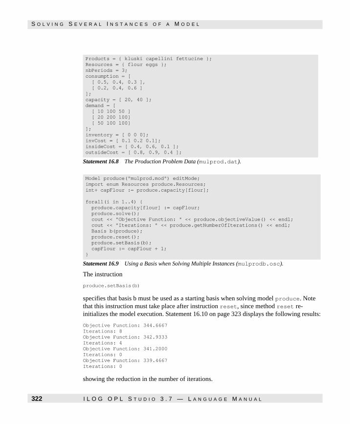
S O L V I N G S E V E R A L I N S T A N C E S O F A M O D E L
Statement 16.8
Statement 16.8 The Production Problem Data (mulprod.dat).
Statement 16.9
Statement 16.9 Using a Basis when Solving Multiple Instances (mulprodb.osc).
The instruction
produce.setBasis(b)
specifies that basis b must be used as a starting basis when solving model produce. Note that this instruction must take place after instruction reset, since method reset re-initializes the model execution. Statement 16.10 on page 323 displays the following results:
Objective Function: 344.6667 Iterations: 8 Objective Function: 342.9333 Iterations: 4 Objective Function: 341.2000 Iterations: 0 Objective Function: 339.4667 Iterations: 0
showing the reduction in the number of iterations.
Products = { kluski capellini fettucine }; Resources = { flour eggs }; nbPeriods = 3; consumption = [ [ 0.5, 0.4, 0.3 ], [ 0.2, 0.4, 0.6 ] ]; capacity = [ 20, 40 ]; demand = [ [ 10 100 50 ] [ 20 200 100] [ 50 100 100] ]; inventory = [ 0 0 0]; invCost = [ 0.1 0.2 0.1]; insideCost = [ 0.4, 0.6, 0.1 ]; outsideCost = [ 0.8, 0.9, 0.4 ];
Model produce("mulprod.mod") editMode; import enum Resources produce.Resources; int+ capFlour := produce.capacity[flour];
forall(i in 1..4) { produce.capacity[flour] := capFlour; produce.solve(); cout << "Objective Function: " << produce.objectiveValue() << endl; cout << "Iterations: " << produce.getNumberOfIterations() << endl; Basis b(produce); produce.reset(); produce.setBasis(b); capFlour := capFlour + 1; }
322 I L O G O P L S T U D I O 3 . 7 — L A N G U A G E M A N U A L
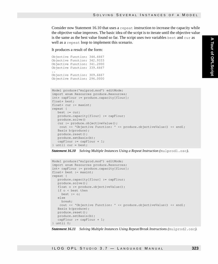
S O L V I N G S E V E R A L I N S T A N C E S O F A M O D E L
A To
ur o
f OP
LS
cript
Consider now Statement 16.10 that uses a repeat instruction to increase the capacity while the objective value improves. The basic idea of the script is to iterate until the objective value is the same as the best value found so far. The script uses two variables best and cur as well as a repeat loop to implement this scenario.
It produces a result of the form:
Objective Function: 344.6667 Objective Function: 342.9333 Objective Function: 341.2000 Objective Function: 339.4667 .. Objective Function: 309.6667 Objective Function: 296.0000
Statement 16.10
Statement 16.10 Solving Multiple Instances Using a Repeat Instruction (mulprod1.osc).
Statement 16.11
Statement 16.11 Solving Multiple Instances Using Repeat/Break Instructions (mulprod2.osc).
Model produce("mulprod.mod") editMode; import enum Resources produce.Resources; int+ capFlour := produce.capacity[flour]; float+ best; float+ cur := maxint; repeat { best := cur; produce.capacity[flour] := capFlour; produce.solve() cur := produce.objectiveValue(); cout << "Objective Function: " << produce.objectiveValue() << endl; Basis b(produce); produce.reset(); produce.setBasis(b); capFlour := capFlour + 1; } until cur = best;
Model produce("mulprod.mod") editMode; import enum Resources produce.Resources; int+ capFlour := produce.capacity[flour]; float+ best := maxint; repeat { produce.capacity[flour] := capFlour; produce.solve(); float o := produce.objectiveValue(); if o < best then best := o; else break; cout << "Objective Function: " << produce.objectiveValue() << endl; Basis b(produce); produce.reset(); produce.setBasis(b); capFlour := capFlour + 1; } until 0;
I L O G O P L S T U D I O 3 . 7 — L A N G U A G E M A N U A L 323

O P E N A R R A Y S
The script 16.11 is similar in spirit but uses a break instruction to terminate the repeat loop. Finally, script 16.12 illustrates how to use a while loop, a break instruction, and the dual values of the constraint to perform the same task.
Open Arrays
Assume now that we are interested in storing all the solutions of the queens problems. A possible, but inefficient, solution would consist of counting the solutions, declaring an array of the appropriate size, and then filling the array by solving the problem again. A more elegant and efficient solution consists of using an open array. An open array is an array that grows or shrinks dynamically at runtime.
Statement 16.12
Statement 16.12 Solving Multiple Instances Using the Dual Values (mulprod3.osc).
Statement 16.13
Statement 16.13 A Script to Store All Solutions (storequeens.osc)
Model produce("mulprod.mod") editMode; import enum Resources produce.Resources; int+ capFlour := produce.capacity[flour]; while 1 do { produce.capacity[flour] := capFlour; produce.solve(); cout << "Objective Function: " << produce.objectiveValue() << endl; float sumDual := sum(t in produce.Periods) produce.cap[flour,t].dual; if sumDual > -1e-8 then break; Basis b(produce); produce.reset(); produce.setBasis(b); capFlour := capFlour + 1; };
Model m("nqueens.mod","nqueens.dat"); int nb := 0; Open int solution[1..0,1..m.n]; while m.nextSolution() do { nb := nb + 1; solution.addh(); forall(i in 1..m.n) solution[nb,i] := m.queens[i]; } forall(s in 1..nb) { forall(i in 1..m.n) { cout << "queens[" << i << "] = "; cout << m.solution[s,i] << endl; } cout << endl; }
324 I L O G O P L S T U D I O 3 . 7 — L A N G U A G E M A N U A L

S E Q U E N C E S O F M O D E L S
A To
ur o
f OP
LS
cript
The script depicted in Statement 16.13 illustrates how open arrays help in solving the problem. The instruction
Open int solution[1..0,1..m.n];
defines a 2-dimensional open array of integers. Both dimensions of this array are open. Since the first dimension is an empty range in the declaration, the entire array is empty. When a solution is found, the method call
solution.addh();
increases the upper bound of the first dimension of the open array solution by one (addh stands for "add high"). The first time this instruction is executed in the above script, the array solution becomes an array of one element whose only index is 1 and whose value is an array that has not yet been initialized. The instructions
forall(i in 1..m.n) solution[nb,i] := m.queens[i]; }
initializes this dynamically created array in the traditional way. The remaining instructions show how to use open arrays.
Sequences of Models
The functionalities described so far make it possible to describe complex applications, possibly involving several models. The purpose of this section is to illustrate how to sequence models on a small configuration application, known as Vellino's problem. The application is a bin-packing configuration that, given a supply of components and bins of various types, must assign the components to the bins so that the bin constraints are satisfied and the smallest possible number of bins is used. There are five types of components, i.e., glass, plastic, steel, wood, and copper, and three types of bins, i.e., red, blue, green. The bins must obey a variety of configuration constraints.
◆ Containment constraints: these are constraints specifying which components can go into which bins:
1.Red bins cannot contain plastic or steel;
2.Blue bins cannot contain wood or plastic;
3.Green bins cannot contain steel or glass.
◆ Capacity constraints: Certain bin-types have a capacity constraint for certain component- types:
1.Red bins contain at most one wooden component;
2.Green bins contain at most two wooden components.
I L O G O P L S T U D I O 3 . 7 — L A N G U A G E M A N U A L 325

S E Q U E N C E S O F M O D E L S
◆ Requirement constraints: For all bins, there are requirement constraints about the components:
1.Wood requires plastic;
2.Glass excludes copper;
3.Copper excludes plastic.
In addition, we are given an initial capacity for each bin, i.e., red bins have a capacity of 3 components, blue bins of 1 and green bins of 4 and a demand for each component, i.e., 1 glass, 2 plastic, 1 steel, 3 wood, and 2 copper components.
The strategy to solve this problem consists of generating all the possible bin configurations and then to choose the smallest number of them that meet the demand. This strategy is implemented using a script vellino.osc depicted in Statement 16.14 on page 327 and two models genBin.mod and chooseBin.mod depicted in Statement 16.15 on page 327 and Statement 16.17 on page 328. Model genBin.mod specifies how to generate the bin configurations: It is a constraint program using logical combinations of constraints. Model chooseBin.mod is an integer program that chooses and minimizes the number of bins.
The model chooseBin.mod that describes the integer program is more involved. First note the instructions
import enum Colors; import enum Components;
that imports the enumerated types from the script language. This is necessary so that enumerated values have the same meaning in the two models and the script.
Note: The models have their own scope and hence would have different enumerated types if no import declaration is used.
326 I L O G O P L S T U D I O 3 . 7 — L A N G U A G E M A N U A L

S E Q U E N C E S O F M O D E L S
A To
ur o
f OP
LS
cript
Statement 16.14
Statement 16.14 A Script to Solve Vellino's Problem (vellino.osc)
Statement 16.15
Statement 16.15 Generating the Bins in Vellino's Problem (genBin.mod)
Statement 16.16
Statement 16.16 Data for Vellino's Problem (genBin.dat)
Model bin("genBin.mod","genBin.dat"); import enum Colors bin.Colors; import enum Components bin.Components; Model pro("chooseBin.mod");
int nbSol := 0; while bin.nextSolution() do { pro.bin.addh(); pro.bin[nbSol].c := bin.c; forall(c in Components) pro.bin[nbSol].n[c] := bin.n[c]; nbSol := nbSol + 1; } pro.nbBin := nbSol;
if pro.solve() then { cout << "Solution at cost: " << pro.objectiveValue() << endl; forall(i in 0..nbSol-1) if pro.produce[i] >= 1 then { cout << "produce " << pro.produce[i] << " units of bin " << endl; cout << " color: " << pro.bin[i].c << endl; forall(c in Components) if pro.bin[i].n[c] > 0 then cout << " " << c << ": " << pro.bin[i].n[c] << endl; } }
enum Colors ...; enum Components ...; int capacity[Colors] = ...; int maxCapacity = max(c in Colors) capacity[c]; var Colors c; var int n[Components] in 0..maxCapacity; solve { 0 < sum(c in Components) n[c] <= capacity[c]; c = red => n[plastic] = 0 & n[steel] = 0 & n[wood] <= 1; c = blue => n[plastic] = 0 & n[wood] = 0; c = green => n[glass] = 0 & n[steel] = 0 & n[wood] <= 2; n[wood] >= 1 => n[plastic] >= 1; n[glass] = 0 \/ n[copper] = 0; n[copper] = 0 \/ n[plastic] = 0;};
Colors = { red, blue, green }; Components = { glass, plastic, steel, wood, copper }; capacity = [ 3, 1, 4];
I L O G O P L S T U D I O 3 . 7 — L A N G U A G E M A N U A L 327

S E Q U E N C E S O F M O D E L S
Statement 16.17
Statement 16.17 Choosing the Bins in Vellino's Problem (chooseBin.mod)
The other novel concept comes from the instructions
struct Bin { Colors c; int n[Components]; }; Open int nbBin; Open Bin bin[int+];
that define an open integer and an open array. These data structures are used by the script to store the results of the model genBin.mod.
Integer nbBin represents the number of bins, while array bin will store the various bin configurations. A bin is represented by its color and by the number of its components. The rest of the model should not raise much difficulty.
It is interesting to study the script in detail at this point. The instructions
Model bin("genBin.mod","genBin.dat"); import enum Colors bin.Colors; import enum Components bin.Components; Model pro("chooseBin.mod");
declare the models and import the enumerated types; these enumerated types are in fact imported as well by model pro.
import enum Colors; import enum Components; struct Bin { Colors c; int n[Components]; }; Open int nbBin; Open Bin bin[int+];
range R 0..nbBin-1;
int demand[Components] = [ 2, 4, 3, 6, 4 ]; int maxDemand = max(c in Components) demand[c];
var int produce[R] in 0..maxDemand;
minimize sum(b in R) produce[b] subject to { forall(c in Components) sum(b in R) bin[b].n[c] * produce[b] = demand[c]; };
Note: When a model contains open data, it is automatically opened in edit mode, since these data structures must be initialized.
328 I L O G O P L S T U D I O 3 . 7 — L A N G U A G E M A N U A L

C O L U M N G E N E R A T I O N
A To
ur o
f OP
LS
cript
The instructions:
int nbSol := 0; while bin.nextSolution() do { pro.bin.addh(); pro.bin[nbSol].c := bin.c; forall(c in Components) pro.bin[nbSol].n[c] := bin.n[c]; nbSol := nbSol + 1; } pro.nbBin := nbSol;
enumerate all the bin configurations and store them in the bin array in model pro. Note the instruction
pro.bin.addh();
to increase the size of the open array and the standard way of accessing these data structures. Once this step is completed, the second model is executed and the solution
Solution at cost: 8 produce 1 units of bin color: red glass: 2 produce 3 units of bin color: blue steel: 1 produce 1 units of bin color: green copper: 4 produce 2 units of bin color: green plastic: 1 wood: 2 produce 1 units of bin color: green plastic: 2 wood: 2
is displayed.
Column Generation
This section concludes the tour of OPLScript by presenting a column generation application: the cutting-stock algorithm of Gilmore and Gomory. The problem consists of cutting big wood boards into small shelves to meet the customer demands while minimizing the number of boards used. A given instance specifies the length of the boards (an integer), the length of the shelves (integers), and the demand for each shelf type (integers as well). The complexity in this application is that it is not practical to generate all the possible configurations: in practical applications, there are so many possible cutting configurations that they cannot even be stored because the boards are large and there are many shelves whose size may be
I L O G O P L S T U D I O 3 . 7 — L A N G U A G E M A N U A L 329

C O L U M N G E N E R A T I O N
rather small. The basic idea behind the column generation approach consists of starting with a set of configurations and then to use the optimal solution to the (linear relaxation of the) simplified problem to generate a new configuration that is promising. In this cutting stock application, a column generation consists of solving a knapsack problem: the capacity constraint makes sure that a legal configuration is generated, while the objective function aims at finding a configuration whose associated variable would enter the basis. This process is iterated until no column can be generated. The upward rounding of the solution is generally considered of sufficient quality.
Statements 16.18 and 16.19 depict a script for this application, while Statements 16.21 and 16.22 show the models. There are a number of interesting features of OPLScript illustrated in this application, as will become clear shortly.
data "cut.dat";
specifies that the data initializations needed by the script may be found in the file cut.dat. Those that are not needed are ignored. The instructions
int nbConfig := -1; Open int+ config[0..nbConfig,Shelves]; forall(i in Shelves) { nbConfig := nbConfig+1; config.addh(); forall(j in Shelves) config[nbConfig,j] := 0; config[nbConfig,i] := boardLength/shelf[i]; }
declares an open array config to store the configuration and initializes it with a first set of configurations, one for each shelf.
The instructions
repeat { chooseC.solve(); forall(i in Shelves) generateC.cost[i] := chooseC.meet[i].dual; generateC.solve(); if generateC.objectiveValue() < -1e-5 then { nbConfig := nbConfig + 1; config.addh(); forall(j in Shelves) config[nbConfig,j] := generateC.use[j]; chooseC.reset(); generateC.reset(); } else break; } until 0;
are the core of the script. The first line chooseC.solve() selects the optimal set of configurations from the subset available. The lines
forall(i in Shelves) generateC.cost[i] := chooseC.meet[i].dual;
330 I L O G O P L S T U D I O 3 . 7 — L A N G U A G E M A N U A L

C O L U M N G E N E R A T I O N
A To
ur o
f OP
LS
cript
generateC.solve();
initialize the objective function for the column generation model using the values of the dual variables. The dual values are used to compute the cost associated with the current configuration in the current basis of Model chooseC. When the objective value of the knapsack problem is negative, then the new configuration will enter the basis and the lines
nbConfig := nbConfig + 1; config.addh(); forall(j in Shelves) config[nbConfig,j] := generateC.use[j]; chooseC.reset(); generateC.reset();
add a new configuration using the result of the knapsack and resets the models. Otherwise, the solution is provably optimal. Note that the core of the script can be improved by using a (partial) basis as starting point for the choice of configurations in all but the first iteration.
This part of the script then becomes
repeat { chooseC.solve(); Basis bc(chooseC); forall(i in Shelves) generateC.cost[i] := chooseC.meet[i].dual; generateC.solve(); if generateC.objectiveValue() < -1e-5 then { nbConfig := nbConfig + 1; config.addh(); forall(j in Shelves) config[nbConfig,j] := generateC.use[j]; chooseC.reset(); chooseC.setBasis(bc); generateC.reset(); } else break; } until 0;
and the implementation takes care of extending this partial basis into a full basis for the extended problem. The rest of the statement (see Statement 16.19 on page 333) computes and pretty-prints the result that is obtained by rounding up the linear programming solution. Note that OPLScript provides many of the formatting features of C++ on streams.
Finally, it is useful to discuss the two models that describe a linear program (to select a subset of the configurations) and an integer program (a knapsack program to generate a new configuration).
I L O G O P L S T U D I O 3 . 7 — L A N G U A G E M A N U A L 331

N O T E S A N D R E F E R E N C E S
The instructions
import int nbConfig; import int+ config[0..nbConfig,1..nbShelves];
indicates that the model chooseC in file chooseConfigs.mod imports nbConfig and the open array config from the script. These instructions avoid having to copy the set of configurations from the script to the model at each iteration.
Notes and References
The Vellino problem is taken from the [28] and is a typical example of applications that require sequencing several models. The script for Gomory and Gilmore's cutting-stock application was inspired by an AMPL script for the same problem.
Statement 16.18
Statement 16.18 A Script For Gilmore and Gomory's Cutting Stock (Part I) (gomory.osc)
data "cut.dat";
int+ boardLength := ...; int nbShelves := ...; range Shelves 1..nbShelves; int shelf[Shelves] := ...; int nbConfig := -1; Open int+ config[0..nbConfig,Shelves]; forall(i in Shelves) { nbConfig := nbConfig+1; config.addh(); forall(j in Shelves) config[nbConfig,j] := 0; config[nbConfig,i] := boardLength/shelf[i]; } Model chooseC("chooseConfigs.mod","cut.dat"); Model generateC("generateConfigs.mod","cut.dat"); repeat { chooseC.solve(); forall(i in Shelves) generateC.cost[i] := chooseC.meet[i].dual; generateC.solve(); if generateC.objectiveValue() < -1e-5 then { nbConfig := nbConfig + 1; config.addh(); forall(j in Shelves) config[nbConfig,j] := generateC.use[j]; chooseC.reset(); generateC.reset(); } else break; } until 0;
332 I L O G O P L S T U D I O 3 . 7 — L A N G U A G E M A N U A L

N O T E S A N D R E F E R E N C E S
A To
ur o
f OP
LS
cript
Statement 16.19
Statement 16.19 A Script For Gilmore and Gomory's Cutting Stock (Part II) (gomory.osc)
Statement 16.20
Statement 16.20 Data For a Cutting Stock Problem (cut.dat)
Statement 16.21
Statement 16.21 A Model for Choosing Cutting Stock Configurations (chooseConfigs.mod)
range Configs 0..nbConfig; int cuti[p in Configs] := ftoi(ceil(chooseC.cut[p])); int obj := sum(p in Configs) cuti[p]; cout << "Solution with Cost: " << obj << endl << endl; cout << " "; forall(w in Shelves) cout << setWidth(6) << shelf[w];cout << endl << endl; forall(p in Configs) { cout << "cut " << setAdjustField(adjustLeft) << setWidth(4) << cuti[p]; cout << " of "; cout << setAdjustField(adjustRight); forall(w in Shelves) cout << setWidth(6) << config[p,w]; cout << endl; }
boardLength = 100; nbShelves = 4; shelf = [ 45 36 31 14 ]; demand = [ 97 610 395 211 ];
int+ boardLength = ...; int nbShelves = ...; range Shelves 1..nbShelves; int shelf[Shelves] = ...; int demand[Shelves] = ...;
import int nbConfig; import int+ config[0..nbConfig,Shelves]; range Configs [0..nbConfig];
constraint meet[Shelves]; var float+ cut[Configs]; minimize sum(j in Configs) cut[j] subject to forall(i in Shelves) meet[i]: sum(j in Configs) config[j,i] * cut[j] >= demand[i];
I L O G O P L S T U D I O 3 . 7 — L A N G U A G E M A N U A L 333

N O T E S A N D R E F E R E N C E S
Statement 16.22
Statement 16.22 A Model for Generating New Cutting Stock Configurations (generateConfigs.mod)
int+ boardLength = ...; int nbShelves = ...; range Shelves 1..nbShelves; int shelf[Shelves] = ...; int demand[Shelves] = ...; Open float cost[Shelves]; var int use[Shelves] in 0..boardLength; minimize 1 - sum(i in Shelves) cost[i]*use[i] subject to sum(i in Shelves) shelf[i] * use[i] <= boardLength;
334 I L O G O P L S T U D I O 3 . 7 — L A N G U A G E M A N U A L

C H A P T E R
OP
LS
cript in
Dep
th
17
OPLScript in Depth
This chapter describes OPLScript in more detail. It reviews its syntax and discusses its functionalities. Since OPLScript shares many of its data modeling features with OPL, this chapter mostly focuses on the novel aspects of OPLScript compared to OPL.
Commands
The syntax of a script is depicted in Partial Grammar 17.1 on page 337, while Table 17.1 on page 338 lists the keywords of OPLScript. A script is a sequence of commands. These commands can be of various types: declarations, simple instructions, and compound instructions.
I L O G O P L S T U D I O 3 . 7 — L A N G U A G E M A N U A L 335

C O M M A N D S
Declarations
Declarations in OPLScript are mostly similar to those of OPL. Both type and data declarations are supported.
For instance, the excerpt
struct Result { int capacity; float obj; int iterations; }; Result res[1..4];
forall(i in 1..4) { produce.capacity[flour] := capFlour; produce.solve(); res[i].capacity := capFlour; res[i].obj := produce.objectiveValue(); res[i].iterations := produce.getNumberOfIterations(); produce.reset(); capFlour := capFlour + 1; }
shows how an array of records can be declared to store the results of multiple instances of the same problem. There are a few syntactic differences in OPLScript declarations that are important to mention. Data declarations use a colon before their initializations as in
int a := 1;
and set declarations must use the keyword setof (not braces) as in
setof(int) s := {1,2,3};
In addition, OPLScript offers new objects such as models, open arrays, files, basis, and import declarations. These will be reviewed independently later in this chapter.
336 I L O G O P L S T U D I O 3 . 7 — L A N G U A G E M A N U A L
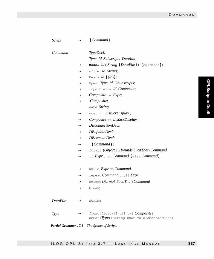
OP
LS
cript in
Dep
th
C O M M A N D S
Partial Grammar 17.1
Partial Grammar 17.1 The Syntax of Scripts
Script → {Command}
Command TypeDecl;
Type Id Subscripts DataInit;
→ Model Id ( String {DataFile}) [editmode];
→ ofile Id String;
→ Basis Id [(Id)];
→ Open Type Id OSubscripts;
→ import enum Id Composite;
→ Composite := Expr;
→ Composite;
data String
→ cout << ListScrDisplay ;
→ Composite << ListScrDisplay ;
→ DBconnectionDecl;
→ DBupdateDecl;
→ DBexecuteDecl;
→ {{Command}}
→ forall (Object in Bounds SuchThat) Command
→ if Expr then Command [else Command]
→ while Expr do Command
→ repeat Command until Expr;
→ select (Formal SuchThat) Command
→ break;
DataFile → String
Type → float|float+|int|int+| Composite|setof(Type)|String|char|void|AbstractModel
I L O G O P L S T U D I O 3 . 7 — L A N G U A G E M A N U A L 337

C O M M A N D S
Table 17.1 Reserved Words of OPLScript.
AbstractModel adjustLeft adjustRight Basis
adjustInternal break by cout
BasisStatus DBconnection DBexecute DBmapping
data DBupdate decreasing diff
DBread do editMode else
display enum fixed float
endl from if import
forall increasing infinity int
in max maxint min
inter Model not ofile
mod ordered piecewise prod
Open repeat scientific select
range setAdjustField setFloatField setof
set setWidth string struct
setPrecision SheetConnection symdiff then
subset SheetRead until SheetWrite
union sum while
338 I L O G O P L S T U D I O 3 . 7 — L A N G U A G E M A N U A L
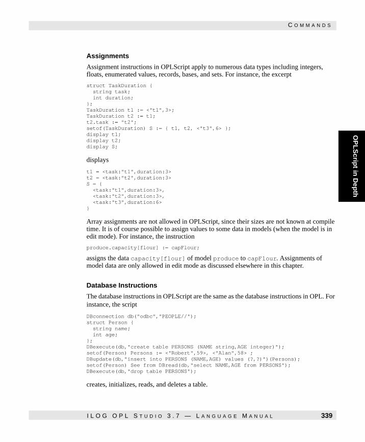
OP
LS
cript in
Dep
th
C O M M A N D S
Assignments
Assignment instructions in OPLScript apply to numerous data types including integers, floats, enumerated values, records, bases, and sets. For instance, the excerpt
struct TaskDuration { string task; int duration; }; TaskDuration t1 := <"t1",3>; TaskDuration t2 := t1; t2.task := "t2"; setof(TaskDuration) S := { t1, t2, <"t3",6> }; display t1; display t2; display S;
displays
t1 = <task:"t1",duration:3> t2 = <task:"t2",duration:3> S = { <task:"t1",duration:3>, <task:"t2",duration:3>, <task:"t3",duration:6> }
Array assignments are not allowed in OPLScript, since their sizes are not known at compile time. It is of course possible to assign values to some data in models (when the model is in edit mode). For instance, the instruction
produce.capacity[flour] := capFlour;
assigns the data capacity[flour] of model produce to capFlour. Assignments of model data are only allowed in edit mode as discussed elsewhere in this chapter.
Database Instructions
The database instructions in OPLScript are the same as the database instructions in OPL. For instance, the script
DBconnection db("odbc","PEOPLE//"); struct Person { string name; int age; }; DBexecute(db,"create table PERSONS (NAME string,AGE integer)"); setof(Person) Persons := <"Robert",59>, <"Alan",58> ; DBupdate(db,"insert into PERSONS (NAME,AGE) values (?,?)")(Persons); setof(Person) See from DBread(db,"select NAME,AGE from PERSONS"); DBexecute(db,"drop table PERSONS");
creates, initializes, reads, and deletes a table.
I L O G O P L S T U D I O 3 . 7 — L A N G U A G E M A N U A L 339

C O M M A N D S
It is also interesting to reconsider one more time the house problem to illustrate how the database instructions can take place in the script language. Statement 17.1 depicts the script, while Statement 17.2 on page 341 depicts the model. The model is almost similar to the one given in Statement 4.1 on page 76, the difference being that the set of tasks and their durations are imported. The script contains database instructions similar to those used in the model given in Statement 11.2 on page 203.
Statement 17.1
Statement 17.1 The Script with Database Instructions for the House Problem (house2db.osc).
DBconnection db("odbc","AHOUSE//"); struct TaskDuration { string Task; int duration; }; setof(TaskDuration) td from DBread(db,"select NAME,DURATION from HTASK"); setof(string) Tasks := { t | <t,d> in td }; int duration[Tasks]; forall(<t,d> in td) duration[t] := d;
struct Schedule { string task; int startTime; int endTime; }; Model m("house2db1.mod"); m.solve(); setof(Schedule) resultSet := { <t,m.a[t].start,m.a[t].end> | t in Tasks };
DBexecute(db, "create table res2 (task string, startTime integer, endTime integer)");DBupdate(db,"insert into res2 (task, startTime, endTime) values (?,?,?)") (resultSet);
340 I L O G O P L S T U D I O 3 . 7 — L A N G U A G E M A N U A L

OP
LS
cript in
Dep
th
C O M M A N D S
Statement 17.2
Statement 17.2 The House Model for a Script (house2db2.mod).
Blocks
OPLScript supports blocks of instructions. A block opens a scope and consists of a sequence of instructions enclosed in between braces. The script
int a := 3; { int a := 4; cout <<"a = " << a << endl; } cout << "a = " << a << endl;
illustrates the use of a block and it displays
a = 4; a = 3;
Note that no semicolon is needed to terminate the block. Blocks are especially useful in conjunction with conditionals and loops.
import {string} Tasks; import int duration[Tasks];
scheduleHorizon = 30; Activity a[t in Tasks](duration[t]);
DiscreteResource budget(29000);
minimize a["moving"].end subject to { a["masonry"] precedes a["carpentry"]; a["masonry"] precedes a["plumbing"]; a["masonry"] precedes a["ceiling"]; a["carpentry"] precedes a["roofing"]; a["ceiling"] precedes a["painting"]; a["roofing"] precedes a["windows"]; a["roofing"] precedes a["facade"]; a["plumbing"] precedes a["facade"]; a["roofing"] precedes a["garden"]; a["plumbing"] precedes a["garden"]; a["windows"] precedes a["moving"]; a["facade"] precedes a["moving"]; a["garden"] precedes a["moving"]; a["painting"] precedes a["moving"];
capacityMax(budget,0,15,20000);
forall(t in Tasks) a[t] consumes(1000*duration[t]) budget; };
I L O G O P L S T U D I O 3 . 7 — L A N G U A G E M A N U A L 341

C O M M A N D S
Conditionals
OPLScript supports traditional conditional instructions. The excerpt
int a := 3; if a > 3 then cout << "a is greater than 3 "; else cout << "a is not greater than 3 ";
illustrates this instruction. The else part of the conditional can be omitted as usual. Blocks should be used when several instructions must be executed as in
int a := ...; int b := ...; if a > b then { cout << "a is greater than b "; cout << "a: " << a << endl; cout << "b: " << b << endl; }
Loops
OPLScript supports three main iterative constructs: while-loops, repeat-loops, and for-loops. The for-loops are a simplified form of the for-construct in OPL: they only involve one parameter and, optionally, a condition. The excerpt
forall(t in m.Tasks) cout << m.act[t].start << endl;
illustrates a for-loop in OPLScript. Of course, a block can be used as the body of for-loop as in
forall(t in m.Tasks) { cout <<"Task "<< t << ": "; cout << m.act[t].start << endl; }
A while-loop executes an instruction while a condition holds. For instance, the excerpt
int l := 0; int u := 10; while l < u do { l := l + 1; u := u - 1; }
performs five iterations. A repeat-loop executes an instruction until a condition holds. For instance, the excerpt
342 I L O G O P L S T U D I O 3 . 7 — L A N G U A G E M A N U A L

OP
LS
cript in
Dep
th
C O M M A N D S
int l := 0; int u := 10; repeat { l := l + 1; u := u - 1; } until l >= u;
also performs five iterations. Loops can be terminated early by using instruction break. For instance, the excerpt
forall(i in 1..10) { if i = 5 then break; else cout << "." } cout << endl;
depicts a for-loop that terminates during the fifth iteration. The break instruction only terminates the innermost loop. For instance, in the excerpt
forall(j in 1..2) { forall(i in 1..10) { if i = 5 then break; else cout << "." } cout << endl; }
the outermost loop is executed twice and each innermost loop is terminated in its fifth iteration.
The data Instruction
The data instruction reads a data file that contains the initial value of some data items. The initial values are used if needed when a data item with an off-line initialization is encountered. Data items mentioned in data files but not present in the script, are ignored. The excerpt
data "cut.dat";
int+ boardWidth := ...; int nbShelves := ...; range Shelves 1..nbShelves; int shelf[Shelves] := ...;
simply states to include the data file cut.dat and declare some data with off-line initialization. These data are initialized using the values specified in file cut.dat. Note that the data file must come before the declarations and that several data instructions may be specified as in
I L O G O P L S T U D I O 3 . 7 — L A N G U A G E M A N U A L 343

M O D E L S
data "cut1.dat"; data "cut2.dat"; int+ boardWidth := ...; int nbShelves := ...; range Shelves 1..nbShelves; int shelf[Shelves] := ...;
The include Instruction
The OPLScript include instruction includes a script in another script. It expects a string literal as argument.
For example, the script dichotest.osc includes another script.
Model mt("../scheduler/bridge.mod","../scheduler/bridge.dat");include "dichop.osc";dicho(mt,0,150);
If the file dichop.osc is not present in the path stated in the OPL Studio option Miscellaneous/OPL and OPLScript Include Path, OPL searches for it in the directory in which dichotest.osc resides and then in the current working directory.
Models
Models are the main interface between OPL and OPLScript. This section details the concept of a model in OPLScript.
Model Declarations
A model is declared in OPLScript by specifying a model file and a (possibly empty) list of data files. For instance, the excerpt
Model m("queens.mod","queens.dat");
declares a model m composed of a model file queens.mod and of a data file queens.dat. Note that the string must be given explicitly in the declaration (i.e., string expressions are not allowed) to make sure that the script is well-typed. Models can also be declared in edit mode, as in
Model m("queens.mod","queens.dat") editMode;
so that some of the instance data can be modified. When a model is declared in edit mode, only enumerated types, open data, data with offline and file initialization are available for inspection and modification. Otherwise any other kinds of data are available for inspection but cannot be modified. Models with open data are always in edit mode since the script is expected to supply values for the open objects before execution. Method declare, applied on a model in edit mode, computes, and makes accessible for inspection, the remaining data.
344 I L O G O P L S T U D I O 3 . 7 — L A N G U A G E M A N U A L

OP
LS
cript in
Dep
th
M O D E L S
Model Data
The data in the model (e.g., arrays and variables) can be accessed as the fields of a record. For instance, the script
Model m("queens.mod","queens.dat"); m.solve(); forall(i in m.n) cout << "queens[" << i << "] = " << m.queens[i] << endl;
illustrates how to access data in a model. The expression m.n denotes the integer n in model m, while expression m.queens[i] denotes element i of array queens in model m. There are of course restrictions on when a data can be accessed. Only enumerated types, open data, data with offline and file initialization can be accessed in edit mode and variables and activities can only be accessed when a solution has been found.
Model Methods
A variety of predefined methods are available on models and Table 17.2 on page 346 depicts their names, their signatures, and their informal meanings. A method is invoked by using, after the model name, a dot, the method name, and the method parameters between parentheses. The excerpt
m.declare(); if m.nextSolution() then cout << "time: " << m.getTime() << endl;
illustrates the methods declare, nextSolution, and getTime. We now review some of these methods in more detail.
Method solve is used to obtain a solution to a model (decision problem) or an optimal solution (optimization problem). Method nextSolution is used to obtain a sequence of solutions. For instance, the excerpt
Model m("queens.mod","queens.dat"); while m.nextSolution() do { forall(i in m.n) cout << "queens[" << i << "] = " << m.queens[i] << endl; cout << endl; }
shows how to display all the solutions to the queens problem. In the case of optimization problems, this method returns a sequence of solutions found during the search for the optimal solution. The objective value of each element in this sequence is better than the objective values of its predecessors.
For instance, the script
Model m("bridge.mod"); while m.nextSolution() do cout << m.objectiveValue() << endl;
I L O G O P L S T U D I O 3 . 7 — L A N G U A G E M A N U A L 345

M O D E L S
displays the objective value of all solutions found when solving the bridge problem. Since this is a minimization problem, the objective values of these solutions are guaranteed to be decreasing.
Table 17.2 Methods on Models.
Method Signature Semantics
declare () Declares the computed data
getBasis () Returns the basis of the solution
getLastIterationResult () Returns the CPLEX solution type (the same as the CPLEX output parameter, CPXsolninfo(), solntype). The values can be:0 - the model has no solution 1 - the model has a simplex basis2 - the model has a solution but no basis
getMathematicalSolutionStatus () Returns the CPLEX solution status. This is the same as the CPLEX return code function CPXgetstat(). The status codes can be found in the CPLEX Reference Manual, Appendix B “Solution Status Codes”.
getNumberOfChoicePoints () Returns the number of choice points
getNumberOfConstraints () Returns the number of constraints
getNumberOfIterations () Returns the number of LP iterations
getNumberOfFails () Returns the number of failures
getNumberOfVariables () Returns the number of variables
getTime () Returns the CPU time in seconds
isDualFeasible () Returns 1 if the current solution is dual feasible (the same as the CPLEX output parameter CPXsolninfo(), dfeasind). Note that a false return value does not necessarily mean that the solution is not feasible. It simply means that the relevant algorithm was not able to conclude it was feasible when it terminated.
346 I L O G O P L S T U D I O 3 . 7 — L A N G U A G E M A N U A L

OP
LS
cript in
Dep
th
M O D E L S
isOptimal () Returns 1 if the solution is proved optimal (if CPXgetstat returns CPX_STAT_OPTIMAL, or CPXMIP_OPTIMAL, or CPXMIP_OPTIMAL_TOL). The CPLEX status codes can be found in the CPLEX Reference Manual, Appendix B “Solution Status Codes”. Returns zero if no solution exists.
isPrimalFeasible () Returns 1 if the current solution is primal feasible (the same as the CPLEX output parameter CPXsolninfo(), pfeasind). Note that a false return value does not necessarily mean that the solution is not feasible. It simply means that the relevant algorithm was not able to conclude it was feasible when it terminated.
nextSolution () Returns the next solution of the model
objectiveValue () Returns the objective value of the solution
reset () Resets the model in its initial state
restore () Restore the last solution found for the model
setBasis (Basis) Specifies a starting basis for LPs
setExportFile (string) Specifies an export file for CPLEX
setFailLimit (Int) Specifies a limit on the number of failures
setFloatParameter (string,float) Specifies the value of a float parameter
setIntegerParameter (string,Int) Specifies the value of an integer parameter
setOrLimit (Int) Specifies a limit on the number of choice points
setStringParameter (string,string) Specifies the value of a string parameter
setTimeLimit (Int) Specifies a limit on CPU time in seconds. This limits only the user’s search procedure and has no influence on the models solved by CPLEX or on the default search procedure.
solve () Solves the model
stateConstraint () Declares the constraints
unsetLimit () Resets all the limits
Table 17.2 Methods on Models. (Continued)
I L O G O P L S T U D I O 3 . 7 — L A N G U A G E M A N U A L 347

M O D E L S
Note that for linear programming and mixed integer programming (assuming that CPLEX MIP is used as the underlying solver), method nextSolution only returns the optimal solution.
Method restore is used to restore the last found solution. Consider the excerpt
Model m("bridge.mod"); while m.nextSolution() do cout << m.objectiveValue() << endl; m.restore(); cout << m.objectiveValue() << endl;
Method restore restores, for model m, the last solution found by method nextSolution. Without this method call, the last instruction would raise an error, since the last call to nextSolution failed. Method reset re-initializes the model in the same state as after its declaration. If the model was declared in edit mode, method reset makes sure that the model is in edit mode again. This method is useful when solving several instances of the same model. The script
Model produce("mulprod.mod") editMode; import enum Resources produce.Resources; int+ capFlour := produce.capacity[flour];
forall(i in 1..4) { produce.capacity[flour] := capFlour; produce.solve(); cout << "Objective Function: " << produce.objectiveValue() << endl; cout << "Iterations: " << produce.getNumberOfIterations() << endl; produce.reset(); capFlour := capFlour + 1; }
illustrates the solving of several instances of a production problem. Note that method reset re-initializes the model in edit mode so that instruction produce.capacity[flour] := capFlour;, at the beginning of the next iteration, may update the model data.
Method declare is only meaningful in edit mode. It declares all data (including variables and activities) of the models, taking into account the modifications performed in edit mode. These derived data can now be accessed if necessary. Method stateConstraint states the problem constraints. Method objectiveValue was used several times already and returns the objective value of a solution (in the case of an optimization problem). This method raises an error if no solution is available (i.e., if no call to solve and nextSolution was executed successfully).
The next set of methods is useful to parametrize the solver. Method setExportFile specifies an export file for linear programming and mixed integer programming applications. Method setBasis specifies a starting basis for a linear program. Methods setStringParameter, setIntegerParameter, and setFloatParameter may be used to initialize parameters for the solver; the parameters are the same as those available from OPL and OPL Studio. Methods setFailLimit, setOrLimit, and setTimeLimit specify
348 I L O G O P L S T U D I O 3 . 7 — L A N G U A G E M A N U A L

OP
LS
cript in
Dep
th
M O D E L S
limits on the number of failures, the number of choice points, and the time spent in the search procedures. The excerpt
Model p("production.mod"); p.setExportFile("production.lp"); p.setStringParameter("LPmethod","barrierPrimal"); p.setFloatParameter("barEpComp",1e-10); p.solve(); cout << p.objectiveValue() << endl; p.reset(); p.setFloatParameter("barEpComp",1e-6); p.solve(); cout << p.objectiveValue() << endl;
illustrates how to export a file and how to set parameters.
The excerpt
Model produce("mulprod.mod") editMode; import enum Resources produce.Resources; int+ capFlour := produce.capacity[flour];
forall(i in 1..4) { produce.capacity[flour] := capFlour; produce.solve(); cout << "Objective Function: " << produce.objectiveValue() << endl; cout << "Iterations: " << produce.getNumberOfIterations() << endl; Basis b(produce); produce.reset(); produce.setBasis(b); capFlour := capFlour + 1; }
illustrates how to specify a basis for a linear program. The basic idea here is to retrieve the basis of an instance using instruction
Basis b(produce);
and to use it to define a starting point for the next instance as follows
produce.setBasis(b);
Note: The complete list of OPL/CPLEX parameters is available in the OPL Studio User's Manual, Appendix A.
I L O G O P L S T U D I O 3 . 7 — L A N G U A G E M A N U A L 349

M O D E L S
Note that method setBasis is invoked after the model was re-initialized with the method reset. The excerpt
Model m("trolley3.mod"); int fails := 1000; m.setFailLimit(fails); int solved := 0; while m.nextSolution() do { solved := 1; cout << "solution with makespan: " << m.objectiveValue() << endl; m.setFailLimit(m.getNumberOfFails() + fails); } m.setFailLimit(m.getNumberOfFails() + fails); if solved then { m.restore(); cout << "final solution with makespan: " << m.objectiveValue() << endl; }
illustrates how to limit the number of failures. It is important to note that the limits are enforced globally on the execution, not locally to the nextSolution method.
Note that methods setFailLimit, setOrLimit, and setTimeLimit specify, respectively, limits on the number of failures, the number of choice points, and the time spent in the user defined search procedures when Solver is used. These methods have no effect when CPLEX is used. To limit the time spent by CPLEX, use the tiLim floating-point parameter. An example for CPLEX is:
model.setFloatParameter("tiLim",3.12)
The next set of methods return information on the execution. Note that these methods are meaningful only in some contexts and raise errors otherwise. For instance, these methods only apply after a solution was found. In addition, method getBasis is only defined for linear programs. Finally, method unsetLimit removes all limits imposed previously.
350 I L O G O P L S T U D I O 3 . 7 — L A N G U A G E M A N U A L

OP
LS
cript in
Dep
th
O P E N A R R A Y S
Open Arrays
Open arrays are a new data structure often useful in scripting. An open array is an array whose range may increase in size at runtime. This feature is useful in many situations, e.g., when a model receives, as input, the solutions of another model or in column-generation applications.
Partial Grammar 17.2
Partial Grammar 17.2 The Syntax of Open Arrays
The syntax of open arrays is specified in Partial Grammar 17.2. The subscripts of an open array must be a range or an enumerated type. The range specifies the initial range of the array and, as shown previously, this range can be extended during the execution.
Of course, enumerated ranges cannot be extended. Open arrays are all one-dimensional, e.g., a two-dimensional open array is simply an open array of open arrays. Hence the innermost arrays may have different sizes. The range of an open array may be empty initially as in
Open int a[0..-1];
Two methods are available on open arrays: addh and addl. These methods increase the dimension of the open array by increasing the upper or the lower bound of the range. The methods are available with no arguments, in which case the first dimension of the open array is modified, or with one argument, in which case the argument specifies how many elements should be added to the first dimension. For instance, the excerpt
Open int a[0..-1]; a.addh(); a[0] := 4; cout << a[0] << endl;
illustrates how to add an element to an open array. Open arrays also can be queried about their size and their lower and upper bound by using the fields size, low, and high (or up).
Command → Open Type Id OSubscripts ;
OSubscripts → [ OSubscript + ]
OSubscript → Range
→ int+
→ Id
I L O G O P L S T U D I O 3 . 7 — L A N G U A G E M A N U A L 351

L I N E A R P R O G R A M M I N G B A S E S
For instance, the excerpt
Open int a[0..-1]; a.addh(2); cout << "low: " << a.low << endl; cout << "high: " << a.high << endl;
displays
low: 0 high: 1
Open arrays are also available in OPL and are mostly useful in a model (the consumer) that receives, as input, the results of another model (the producer). These two models can be glued together by a script that takes the producer results and stores them in open arrays of the consumer. Open arrays in OPL can be used as standard arrays, except that they cannot be indexed by expressions containing variables. An intermediary array must be created when this functionality is needed. An interesting feature of open arrays is that OPL views them as data with off-line initializations when a model is run independently (i.e., not from a script). This functionality makes it possible to develop, test, and maintain these models independently from the scripts using them, and makes the languages compositional. Consider the simple model
int n = ...; Open int a[1..n]; var int x[1..n] in 1..n; solve { forall(i in 1..n) x[i] = a[i]; };
This model can be executed with a data file containing
n = 5; a = [5, 4, 3, 2, 1];
Linear Programming Bases
Linear programming bases are first-class objects in OPLScript. As seen previously, a basis can be retrieved from a model using the method getBasis and stored in a model (to be used as a starting basis) using the method setBasis. Several Basis objects can be stored without naming each of them. A basis can be declared together with a model as in:
Model m("production.mod"); m.solve(); Basis a(m);
in which case the basis a is initialized with the model basis. A basis can be declared without initialization, as in
Basis a;
352 I L O G O P L S T U D I O 3 . 7 — L A N G U A G E M A N U A L

OP
LS
cript in
Dep
th
O U T P U T F I L E S
and it can be given a value in an assignment, as in
a := m.getBasis();
It is useful to understand how bases work. A basis associates a status with every variable and constraint in a linear program. These variables and constraints are identified by their model names in the basis. When a basis b is used as the starting basis of a model m, each variable and each constraint of the model receives a basis status using basis b. The model names are used to define a mapping between the variables and constraints in the model and in the basis. The basis can be partial, i.e., some variables and/or constraints in the model may not be present in the basis. In this case, the OPL implementation is responsible for assigning them a status.
To access the content of a Basis object, use the print method in an output file.
..... Model gas("gas.mod","gas.dat") editMode;
if (gas.solve()) then { Basis basis := gas.getBasis(); ofile file("z:/ilog/oplst36/examples/opl/bas.txt"); basis.print(file); file.close(); } .....
Output Files
Output files can be declared in OPLScript by simply specifying a file name. For instance, the instruction
ofile f("trace.txt");
opens a file trace.txt. Once an output file has been defined, it can be used in the stream instructions instead of the standard output cout as in
ofile trace("trace.txt"); Open int a[0..-1]; a.addh(); a[0] := 4; trace << a[0] << endl;
Files can be closed using the close method as in:
ofile trace("trace.txt"); Open int a[0..-1]; a.addh(); a[0] := 4; trace << a[0] << endl; trace.close();
I L O G O P L S T U D I O 3 . 7 — L A N G U A G E M A N U A L 353

S T R E A M S
Partial Grammar 17.3
Partial Grammar 17.3 The Syntax of Output Instructions
Streams
OPLScript provides most of the formatting functionalities of C++ output streams. The syntax of the output instructions is shown in Partial Grammar 17.3 on page 354. An output instruction specifies an output stream, i.e., cout or an output file, and a sequence of data to display and/or stream manipulators separated by the terminal <<. The data to be displayed must be of type integer, float, enumerated values, char (e.g., ’a’), or string. The terminal endl displays an end-of-line character. The manipulators setPrecision, setWidth, setFloatField, and setAdjustField have the same meanings as their C++ counterparts. Manipulator setPrecision specifies the precision of floats, setWidth specifies the minimum number of characters to be used for the next numeric or string display, setFloatField specifies whether scientific or fixed notation must be used for floats, and setAdjustField specifies whether the filling must take place on the left, on the right, or internally.
Command → cout << ListScrDisplay ;
→ Composite << ListScrDisplay ;
ListScrDisplay → ScrDisplay { << ListScrDisplay }
ScrDisplay → String
→ Expr
→ Char
→ endl
→ setPrecision (Expr)
→ setWidth (Expr)
→ setFloatField (Id)
→ setAdjustField (AdjustFieldValue)
FloatFieldValue → scientific
→ fixed
AdjustFieldValue → adjustLeft
→ adjustRight
→ adjustInternal
354 I L O G O P L S T U D I O 3 . 7 — L A N G U A G E M A N U A L

OP
LS
cript in
Dep
th
I M P O R T D E C L A R A T I O N S
Import Declarations
Import declarations make it possible to communicate data and types in between models. This section reviews these declarations in more detail.
Import in Scripts
Scripts can import enumerated types from models. For instance, in the excerpt,
Model bin("genBin.mod","genBin.dat"); import enum TheColors bin.Colors; import enum Components bin.Components;
the instruction
import enum TheColors bin.Colors;
imports the enumerated types Colors from model bin and renames it TheColors for use in the script. As a result, it is now possible to use TheColors instead of bin.Colors in the script. It is important to stress that models have their own scope. Hence, if a script and a model contain the same declaration, say,
enum Size {small, medium, large};
these declarations in fact denote different enumerated types and values from one type cannot be assigned to data from the other type. Import declarations must be used to share enumerated types between models and between models and scripts. For instance, the excerpt
Model m("e.mod"); enum Size { small, medium, large}; Size aSize := m.aSize;
is necessarily semantically incorrect, since m.aSize cannot be of the enumerated type Size defined in the excerpt.
Import in Models
Models can also import enumerated types from a script. For instance, the model excerpt
import enum Colors; import enum Components;
shows how to import enumerated types from a script to a model. Note that the enumerated types defined in the script may themselves be imported, in which case the model is actually importing these types from another model.
I L O G O P L S T U D I O 3 . 7 — L A N G U A G E M A N U A L 355

P R E D E F I N E D P R O C E D U R E S
Models can also import open and traditional data. Consider the model
int+ boardLength = ...; int nbShelves = ...; range Shelves 1..nbShelves; int shelf[Shelves] = ...; int demand[Shelves] = ...; import Open config; range Configs [config.low..config.up]; var float+ cut[Configs]; minimize sum(j in Configs) cut[j] subject to forall(i in Shelves) sum(j in Configs) config[j,i] * cut[j] >= demand[i];
The model imports the open array config from a script.
It is also possible to specify the types of imported data. Consider the following variation of the above model.
int+ boardLength = ...; int nbShelves = ...; range Shelves 1..nbShelves; int shelf[Shelves] = ...; int demand[Shelves] = ...; import int+ nbConfig; import int+ config[0..nbConfigs,Shelves]; range Configs [0..nbConfigs]; var float+ cut[Configs]; minimize sum(j in Configs) cut[j] subject to forall(i in Shelves) sum(j in Configs) config[j,i] * cut[j] >= demand[i];
Partial Grammar 17.4
Partial Grammar 17.4 The Syntax of Import Instructions in OPL
The import declarations
import int+ nbConfig; import int+ config[0..nbConfigs,Shelves];
now specify the types of the import data. The main benefit of specifying the types come from the ability to execute and maintain the model independently from the scripts using it. As was the case with open data, import declarations in a model run in isolation are considered data with offline initialization. As a consequence, the above model can be run with a data file assigning values to nbConfig and config as well as the other offline data.
Predefined Procedures
OPLScript also has a predefined procedure srand(int seed) to initialize a generator of pseudo-random numbers. Of course, rand functions can also be used in OPLScript.
Import → import enum Id
→ import Open Id
→ import data Id
→ import Type Id Subscripts
356 I L O G O P L S T U D I O 3 . 7 — L A N G U A G E M A N U A L

OP
LS
cript in
Dep
th
A B S T R A C T M O D E L S
Abstract Models
In relation with first class Model objects, OPLScript supports the Abstract Model, also as a first class object. Abstract models can be thought of as a super class of models. The interface supported by abstract models makes it possible to manipulate models without any knowledge of the actual model instance that it contains. Consequently, the interface is limited to generic operations such as stating the model, solving it, displaying its solution, obtaining the value of the objective function or altering the solver parameters. Given the close relationship between models and abstract models, OPLScript authorizes assignments of model instances to abstract model instances. The excerpt
string m := "queens.mod"; setof(string) dataSet := {"q1.dat","q2.dat"}; forall(d in dataSet) { AbstractModel am := Model(m,d); am.solve(); am.displaySolution(); am.close(); }
solves the queens model once for each data set listed in dataSet. Notice that the forall loop is completely model independent. The applications for abstract models range from sensitivity analysis to generic meta-heuristics and play a crucial role in code reuse when used in conjunction with user defined procedures (see the section User Defined Procedures on page 363). The complete interface for AbstractModel is listed in Table 17.3 on page 362 and is defined as:
◆ int nextSolution()
Computes successive solutions for the OPL model previously loaded by the invoking object. For optimization problems, this member function can be used to obtain a sequence of solutions, each of which improves the best value of the objective function found so far. If the returned value is equal to zero, then the value of the objective function cannot be further improved. In order to retrieve the optimal solution you can use the member function restore. If the first call to nextSolution returns zero, the model has no solution.
I L O G O P L S T U D I O 3 . 7 — L A N G U A G E M A N U A L 357

A B S T R A C T M O D E L S
◆ int solve()
This member function computes the optimal solution of the OPL model previously loaded by the invoking object. If the returned value is equal to zero, the model has no solution.
◆ void reset()
This member function determines the OPL engine to reset the loaded model to its initial state. Thus, any model modifications made by the client code are lost and any references in the client code to model items are no longer valid.
◆ void restore()
This member function restores the last solution found by using the member function nextSolution for the invoking object.
◆ void declare()
This member function instructs the OPL engine to construct and initialize the data structures of the model previously loaded in edit mode. No solving process is taking place. After calling declare, the client code can access/modify data items inside the model.
◆ void close()
Signals that the invoking object will no longer be used by the client code. Hence the memory used by the invoking object is returned to the system. Once this member function has been called, no other member functions may by called by the invoking object.
◆ void stateConstraint()
Instructs the OPL engine to take into account the constraints declared in the model previously loaded in edit mode. No solving process is taking place. This member function will also implicitly call declare. After calling stateConstraint, the client code can access/modify data items inside the model and inspect the named constraints of the model.
◆ void displaySolution()
This member function returns a string containing the result of the execution of the possible displaySolution statements from the OPL model previously loaded and solved.
◆ void displaySolution1(file)
This member function is identical to displaySolution, except that output is sent to the text file passed as argument rather than to stdout.
358 I L O G O P L S T U D I O 3 . 7 — L A N G U A G E M A N U A L

OP
LS
cript in
Dep
th
A B S T R A C T M O D E L S
◆ int objectiveIntValue()
This member function allows the client code to access the value of the objective function in an optimization model. It assumes that the objective function is typed as integer. This member function must be called after a successful call to the nextSolution or solve methods for the invoking object.
◆ float objectiveFloatValue()
This member function allows the client code to access the value of the objective function in an optimization model. It assumes that the objective function is typed as oat. This member function must be called after a successful call to the nextSolution or solve methods for the invoking object.
◆ void setFailLimit(int)
This member function specifies a limit on the number of failures the OPL engine may encounter during the search for a solution. When the limit is reached, the search stops and the current call to the member function solve or nextSolution returns a zero value.
◆ void setTimeLimit(int)
This member function specifies a limit, in seconds, on the CPU time the OPL engine takes to search for a solution. When the limit is reached, the search stops and the current call to the member function solve or nextSolution returns a zero value.
◆ void setOrLimit(int)
This member function specifies a limit on the number of choice points the OPL engine may encounter during the search for a solution. When the limit is reached, the search stops and the current call to the member function solve or nextSolution returns a zero value.
◆ void unsetLimit(void)
This member function unsets any limit a previous call to setFailLimit, setOrLimit, or setTimeLimit could have set on the invoking object.
◆ int getNumberOfFails()
This member function may be used to retrieve the number of failures encountered since the creation of the invoking object, or since the re-initialization of the invoking object by a call to the member function reset.
◆ float getTime()
This member function may be used to retrieve the time elapsed, in seconds, since the creation of the invoking object.
I L O G O P L S T U D I O 3 . 7 — L A N G U A G E M A N U A L 359

A B S T R A C T M O D E L S
◆ Basis getBasis()
This member function obtains the basis of the model stored in the AbstractModel object. The basis is represented by an instance of an object of type Basis. This is valid on LP problem (when CPLEX is used).
◆ int getNumberOfIterations()
This member function may be used to retrieve the number of simplex iterations made so far by the OPL engine associated with the invoking object.
◆ void setBasis(Basis)
This member function is the converse of getBasis. It sets the Basis passed as argument as the initial basis for the model currently loaded in the abstract model. The mapping (association of a status with each variable/constraint) is based on the names of variables/constraints.
◆ int getNumberOfVariables()
This member function may be used to retrieve the number of constrained variables that are used in the OPL model loaded by the invoking object.
◆ int getNumberOfChoicePoints()
This member function may be used to retrieve the number of choice points encountered since the creation of the invoking object, or since the re-initialization of the invoking object by a call to the member function reset.
◆ int getNumberOfConstraints()
This member function may be used to retrieve the number of constraints that occur in the OPL model loaded by the invoking object.
◆ void setExportFile(string)
This member function may be used to write a previously loaded linear model to a file in a to which the model is written. The model is written once solve or nextSolution is called. The argument string indicates the file to which the model is written. The file extension (the characters following the last period in string) is used to infer the format of the file as follows:
● .sav binary SAV file
● .mps MPS format
● .lp LP format
● .rmp MPS format generic names
● .rew MPS format, generic names
● .rlp LP format, generic names
360 I L O G O P L S T U D I O 3 . 7 — L A N G U A G E M A N U A L

OP
LS
cript in
Dep
th
A B S T R A C T M O D E L S
◆ void setOptimizationStep(float)
This member function tells the OPL engine to produce solutions that are at least a step better during the repeated solving of an optimization model. In other words, each call to nextSolution will find a solution that improves the objective by at least the step float.
◆ void setStringParameter(string,string)
This member function may be used in order to specify the value of a string parameter to the OPL engine. The first string argument indicates the parameter name. The second string argument contains the parameter value.
◆ void setIntegerParameter(string,int)
This member function may be used in order to specify the value of an int parameter to the OPL engine. The string argument indicates the parameter name. The int argument contains the parameter value.
◆ void setFloatParameter(string,float)
This member function may be used in order to specify the value of a float parameter to the OPL engine. The string argument indicates the parameter's name. The float argument contains the parameter value.
◆ void setObjValueMax(int)
This member function constrains the OPL engine to search only for solutions with an objective value less than or equal to the integer value int. It assumes that the invoking object is referring to an optimization model with an integer objective function.
◆ void setObjValueMin(int)
This member function constrains the OPL engine to search only for solutions with the objective value greater than or equal to the integer value int. It assumes that the invoking object is referring to an optimization model with an integer objective function.
◆ void setObjFloatValueMax(float)
This member function constrains the OPL engine to search only for solutions with an objective value less than or equal to the oat value float. It assumes that the invoking object is referring to an optimization model with a oat objective function.
◆ void setObjFloatValueMin(float)
This member function constrains the OPL engine to search only for solutions with an objective value greater than or equal to the oat value float. It assumes that the invoking object is referring to an optimization model with a oat objective function.
I L O G O P L S T U D I O 3 . 7 — L A N G U A G E M A N U A L 361

A B S T R A C T M O D E L S
Table 17.3 The AbstractModel Interface: Synopsis
Method Type Short Description
int nextSolution() Finds the next solution
int solve() Solves the model
void reset() Resets the model
void restore() Restores the best solution
void declare() Declares the data structures
void close() Releases the model
void stateConstraint() States the model constraints
void displaySolution() Prints the current solution to the standard output
void displaySolution1(ofile file) Prints the current solution to the file denoted by file
int objectiveIntValue() Returns the objective value
float objectiveFloatValue() Returns the objective value
void setFailLimit(int) Bounds the number of failures
void setTimeLimit(int) Bounds the execution time
void setOrLimit(int) Bounds the number of choice points
void unsetLimit(void) Removes all limits
int getNumberOfFails() Returns the number of failures encountered so far
float getTime() Returns the execution time
Basis getBasis() Returns a snapshot of the current basis (meaningful for linear programs)
int getNumberOfIterations() Returns the number of iterations for the simplex algorithm
void setBasis(Basis) Imposes the basis passed as argument as a starting point
int getNumberOfVariables() Returns the number of variables
int getNumberOfChoicePoints() Returns the number of choice points
int getNumberOfConstraints() Returns the number of constraints
362 I L O G O P L S T U D I O 3 . 7 — L A N G U A G E M A N U A L

OP
LS
cript in
Dep
th
U S E R D E F I N E D P R O C E D U R E S
User Defined Procedures
OPLScript also supports procedural abstraction. It is possible to define procedures that encapsulate processing carried out on various data structures of the script. The focus is on the processing, and algorithms to implement the desired computation. OPLScript, like most procedural languages, supports this abstraction with the concept of procedures or functions taking one or several arguments as input and possibly returning some values. For instance, the excerpt
procedure int stringToInt(string s) { int retVal := 0; char ch := '0'; forall(i in 0..s.length()-1) retVal := retVal * 10 + s.charAt(i).intValue() - ch.intValue(); return retVal; }
implements a conversion routine from a string storing a number in base 10 to its integer representation. The relevant syntax for OPLScript procedures can be found in Partial Grammar 17.5 on page 364.
void setExportFile(string) Specifies an export file for CPLEX
void setOptimizationStep(float) Changes the optimization step
void setStringParameter(string,string) Modifies a CPLEX string parameter
void setIntegerParameter(string,int) Modifies a CPLEX integer parameter
void setFloatParameter(string,float) Modifies a CPLEX floating point parameter
void setObjValueMax(int) Constrains the objective value function
void setObjValueMin(int) Constrains the objective value function
void setObjFloatValueMax(float) Constrains the objective value function
void setObjFloatValueMin(float) Constrains the objective value function
Table 17.3 The AbstractModel Interface: Synopsis (Continued)
I L O G O P L S T U D I O 3 . 7 — L A N G U A G E M A N U A L 363

U S E R D E F I N E D P R O C E D U R E S
Partial Grammar 17.5
Partial Grammar 17.5 The Syntax of Scripts
Script → {Command}
→
ProcDecl → procedure Type DataId ( [ ListProcArg ] ) { { Command } }
ListProcArg → Type DataId [ArrayArgs ] {, Type DataId [ArrayArgs] }
ArrayArgs → [ArrayArg {, ArrayArg } ]
ArrayArg → range | Composite
→
Command TypeDecl;
Type Id Subscripts DataInit;→ Model Id ( String {DataFile}) [editmode];
→ AbstractModel Id (String { DataFile }) [editMode]→ Basis Id [(String)];
→ Open Type Id OSubscripts;
→ import enum Id Composite;
→ Composite := Expr;
→ Composite;
→ data String
→ ProcDecl
→ cout << ListScrDisplay ;
→ Composite << ListScrDisplay ;
→ DeclDBconnectionDecl;
→ DeclDBupdateDecl;→ DeclDBexecuteDecl;
→ {{Command}}→ forall (Object in Bounds SuchThat) Command→ if Expr then Command [else Command]
→ while Expr do Command
→ repeat Command until Expr;
→ select (Formal SuchThat) Command
→ break;
Type → float|float+|int|int+| Composite|setof(Compos-ite)|string|BasisStatus|AbstractModel|void
364 I L O G O P L S T U D I O 3 . 7 — L A N G U A G E M A N U A L
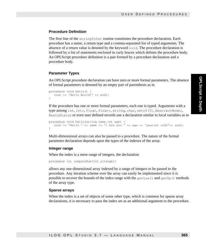
OP
LS
cript in
Dep
th
U S E R D E F I N E D P R O C E D U R E S
Procedure Definition
The first line of the stringToInt routine constitutes the procedure declaration. Each procedure has a name, a return type and a comma-separated list of typed arguments. The absence of a return value is denoted by the keyword void. The procedure declaration is followed by a list of statements enclosed in curly braces which defines the procedure body. An OPLScript procedure definition is a pair formed by a procedure declaration and a procedure body.
Parameter Types
An OPLScript procedure declaration can have zero or more formal parameters. The absence of formal parameters is denoted by an empty pair of parenthesis as in
procedure void hello() { cout << "Hello World!" << endl; }
If the procedure has one or more formal parameters, each one is typed. Arguments with a type among int, int+, float, float+, string, char, setof(T), AbstractModel, BasisStatus or even user defined records use a declaration similar to local variables as in
procedure void hello(string name,int age) { cout << "Hello " << name << "! Are you " << age << "year(s) old?"<< endl;}
Multi-dimensional arrays can also be passed to a procedure. The nature of the formal parameter declaration depends upon the types of the indexes of the array.
Integer range
When the index is a mere range of integers, the declaration
procedure int computeSum(int a[range])
allows any one-dimensional array indexed by a range of integers to be passed to the procedure. Any iteration scheme over the array can easily be implemented since it is possible to recover the bounds of the index range with the getLow() and getUp() methods of the array type.
Sparse arrays
When the index is a set of objects of some other type, which is common for sparse array declarations, it is necessary to pass the index set as an additional argument to the procedure.
I L O G O P L S T U D I O 3 . 7 — L A N G U A G E M A N U A L 365

U S E R D E F I N E D P R O C E D U R E S
The excerpt
procedure int computeSum(setof(string) S,int a[S]) { int s := 0; forall(i in S) s := s + a[i]; return s; } setof(string) Z := {"a","b","c"}; int br[Z] := [1 ,2 ,3 ]; int s2 := computeSum(Z,br);
illustrates this situation. br is a sparse array indexed with a set of strings. In order to pass it to a procedure, the procedure must accept two distinct arguments: one to accommodate the index set, the other for the array. Notice how the procedure declaration states that the formal argument S is a set of strings and reuses the name S in the procedure declaration to specify the type of the second formal argument a. The computeSum procedure so defined is reusable with different arrays defined on various sets of strings.
Parameter Passing Mode
OPLScript supports a single parameter passing mode for procedure arguments called passing by reference. Parameters passed by reference make it possible for the procedure to modify the value of the parameter and to make this change visible to the caller. In a sense, a 'by reference' parameter introduces a name which is a mere alias to an existing object instance of the same type. As a consequence, the code fragment
procedure void foo(int a) { cout << "inside foo(1): " << a << endl; a := a * 10; cout << "inside foo(2): " << a << endl; } int a := 1; cout << "Before foo: " << a << endl; foo(a); cout << "After foo: " << a << endl;
produces the output
Before foo: 1 inside foo(1): 1 inside foo(2): 10 After foo: 10
This parameter passing convention is enforced for all parameter types. Clearly, it is possible to write procedures that modify arrays, sets or structures passed as arguments. The absence of the classic 'by value' parameter passing mode does not penalize users as it is possible to pass literal values to procedures. Indeed, OPLScript simply creates a temporary object that stores the literal value and passes it by reference to the procedure. The excerpt
int val := stringToInt("1234");
illustrates this capability.
366 I L O G O P L S T U D I O 3 . 7 — L A N G U A G E M A N U A L

OP
LS
cript in
Dep
th
P R E P R O C E S S I N G
Procedure Body
The body of a procedure is a sequence of commands like the main body of a script. It is thus possible to declare local variables of any type or even nested procedures as in
procedure int foo(int a) { int tab[i in 1..10] := i; procedure int bar(int b) { return b+1; } return bar(tab[a]) * 2; } cout << foo(5) << endl;
In addition to all the control statements available in OPLScript, procedures can also choose to implement control with recursion as in
procedure int fact(int n) { if n=0 then return 1; else return n*fact(n-1); }
This example illustrates a recursive definition of the well-known mathematical function factorial. It also demonstrates that the 'by reference' parameter passing mode does not penalize the clarity of the statement as OPLScript automatically instantiates a temporary variable to store the result of the expression n-1 that is being passed to the recursive call.
Preprocessing
OPLScript assists in the development of modular scripts by providing a file inclusion facility. It is possible to organize large scripts in several different units, each stored in a separate file. File inclusions can be nested to an arbitrary depth but cannot be recursive or mutually recursive. The excerpt
include "dicho.osc"; Model m("abridge.mod"); dicho(m,0,1000);
with a file "dicho.osc" containing the fragment shown in Statement 17.3 on page 368 provides a clean separation between the generic dichotomic meta-heuristic procedure and the actual user scripts that use it. This facility makes it possible to develop libraries of useful, reusable, script fragments. Note that the dicho procedure takes as input an abstract model and the interval on which to execute the dichotomic search. The body of the procedure is a traditional implementation that ends with a statement to restore the best solution found. Finally, OPLScript uses a straightforward convention for locating the included files.
I L O G O P L S T U D I O 3 . 7 — L A N G U A G E M A N U A L 367

P R E P R O C E S S I N G
OPLScript first attempts to locate the file in the current working directory; then it will look into a semicolon-separated list of paths that can be specified in the graphical user interface.
Statement 17.3
Statement 17.3 A Generic Dichotomic Procedure.
procedure int dicho(AbstractModel m,int low,int up) { int found := 0; int minv := low; int maxv := up; while minv <= maxv do { int value := (minv + maxv) / 2; m.setObjValueMax(value); if (m.nextSolution()) then { maxv := m.objectiveIntValue(); cout << "Solution at cost: " << maxv << endl; maxv := maxv - 1; found := 1; } else { cout << "No solution at cost below: " << value << endl; minv := value + 1; } } if found then m.restore(); return found; }
368 I L O G O P L S T U D I O 3 . 7 — L A N G U A G E M A N U A L

Part IV


Appendixes
Appendix A contains a bibliography.
I L O G O P L S T U D I O 3 . 7 — L A N G U A G E M A N U A L 371

372 I L O G O P L S T U D I O 3 . 7 — L A N G U A G E M A N U A L

A P P E N D I X
A
Bibliography
[1]
A. Aggoun and N. Beldiceanu. Extending CHIP to Solve Complex Scheduling and Packing Problems. In Journées Francophones de Programmation Logique, Lille, France, 1992.
[2]
M. Bartusch. Optimierung von Netzplaenen mit Anordnungsbeziehungen bei Knappen Betriebsmitteln. PhD thesis, Fakultaet fur Mathematik und Informatik, Universitaet Passau, Germany, 1983.
[3]
N. Christofides. Graph Theory: An Algorithmic Approach. Academic Press, New York, 1975.
[4]
A. Colmerauer. An Introduction to Prolog III. Commun. ACM, 28(4):412--418, 1990.
[5]
A. Colmerauer, H. Kanoui, and M. Van Caneghem. Prolog, Bases Theoriques et Développements Actuels. T.S.I. (Techniques et Sciences Informatiques), 2(4):271--311, 1983.
I L O G O P L S T U D I O 3 . 7 — L A N G U A G E M A N U A L 373

[6]
G.B. Dantzig. Linear Programming and Extensions. Princeton University Press, Princeton, N.J., 1963.
[7]
M. Dincbas, H. Simonis, and P. Van Hentenryck. Solving the Car Sequencing Problem in Constraint Logic Programming. In European Conference on Artificial Intelligence (ECAI-88), Munich, Germany, August 1988.
[8]
M. Dincbas, P. Van Hentenryck, H. Simonis, A. Aggoun, T. Graf, and F. Berthier. The Constraint Logic Programming Language CHIP. In Proceedings of the International Conference on Fifth Generation Computer Systems, Tokyo, Japan, December 1988.
[9]
R. Fourer, D. Gay, and B.W. Kernighan. AMPL: A Modeling Language for Mathematical Programming. The Scientific Press, San Francisco, CA, 1993.
[10]
M.R. Garey and D.S. Johnson. Computers and Intractability. W.H. Freeman and Company, New York, 1979.
[11]
R.S Garfinkel and G.L Nemhauser. Integer Programming. John Wiley & Sons, New York, 1972.
[12]
D. Gusfield and R.W. Irving. The Stable Marriage Problem: Structure and Algorithms. The MIT Press, Cambridge, MA, 1989.
[13]
[14]
J. Jaffar and M. Maher. Constraint Logic Programming: A Survey. Journal of Logic Programming, 19/20:503--582, May/July 1994.
[15]
J. Jaffar, S. Michaylov, P.J. Stuckey, and R. Yap. The CLP(ℜ) Language and System. ACM Trans. on Programming Languages and Systems, 14(3):339--395, 1992.
[16]
M.J. Maher. Logic Semantics for a Class of Committed-Choice Programs. In Fourth International Conference on Logic Programming, pages 858--876, Melbourne, Australia, May 1987.
374 I L O G O P L S T U D I O 3 . 7 — L A N G U A G E M A N U A L

[17]
K. McAloon and C. Tretkoff. 2LP: Linear Programming and Logic Programming. In V. Saraswat and P. Van Hentenryck, editors, Principles and Practice of Constraint Programming. The MIT Press, Cambridge, Ma, 1995.
[18]
P. Meseguer. Interleaved Depth-First Search. In Proceedings of the 15th International Joint Conference on Artificial Intelligence, Nagoya, Japan, August 1997.
[19]
W. Older and A. Vellino. Extending Prolog with Constraint Arithmetics on Real Intervals. In Canadian Conference on Computer & Electrical Engineering, Ottawa, 1990.
[20]
C.H. Papadimitriou and K. Steiglitz. Combinatorial Optimization: Algorithms and Complexity. Prentice-Hall, Englewood Cliffs, NJ, 1982.
[21]
B.D. Parrello. CAR WARS: The (Almost) Birth of an Expert System. AI Expert, 3(1):60--64, January 1988.
[22]
J-F. Puget. A C++ Implementation of CLP. In Proceedings of SPICIS'94, Singapore, November 1994.
[23]
J-F. Puget and M. Leconte. Beyond the Glass Box: Constraints as Objects. In Proceedings of the International Symposium on Logic Programming (ILPS-95), Portland, OR, November 1995.
[24]
Roseaux. Programmation linéaire et extensions; problèmes classiques, volume 3 of Exercices et problèmes résolus de Recherche Opérationnelle. Masson, Paris, 1985.
[25]
Ilog SA. Ilog CPLEX 6.0 Reference Manual, 1998.
[26]
Ilog SA. Ilog Planner 3.2 Reference Manual, 1998.
[27]
Ilog SA. Ilog Scheduler 4.4 Reference Manual, 1998.
I L O G O P L S T U D I O 3 . 7 — L A N G U A G E M A N U A L 375

[28]
Ilog SA. Ilog Solver 4.4 Reference Manual, 1998.
[29]
V.A. Saraswat. Concurrent Constraint Programming Languages. PhD thesis, Carnegie-Mellon University, 1989.
[30]
G. Smolka. The Oz Programming Model. In Jan van Leeuwen, editor, Computer Science Today. LNCS, No. 1000, Springer Verlag, 1995.
[31]
P. Van Hentenryck. Constraint Satisfaction in Logic Programming. Logic Programming Series, The MIT Press, Cambridge, MA, 1989.
[32]
P. Van Hentenryck. Constraint Logic Programming. Knowledge Engineering Review, 6(3), 1991.
[33]
P. Van Hentenryck. Scheduling and Packing in the Constraint Language cc(FD). In Intelligent Scheduling. M. Zweben and M. Fox (Eds.), Morgan Kaufmann, 1994.
[34]
P. Van Hentenryck. Encyclopedia of Science and Technology, chapter Constraint Programming. Marcel Dekker, 1997.
[35]
P. Van Hentenryck. The OPL Optimization Programming Language. The MIT Press, Cambridge, Mass., 1999.
[36]
P. Van Hentenryck and J-P. Carillon. Generality Versus Specificity: An Experience with AI and OR Techniques. In Proceedings of the American Association for Artificial Intelligence (AAAI-88), (St. Paul, MN), August 1988. AAAI, Menlo Park, Calif.
[37]
P. Van Hentenryck and Y. Deville. The Cardinality Operator: A New Logical Connective and its Application to Constraint Logic Programming. In Eighth International Conference on Logic Programming (ICLP-91), Paris (France), June 1991.
376 I L O G O P L S T U D I O 3 . 7 — L A N G U A G E M A N U A L

[38]
P. Van Hentenryck and V. Saraswat. Strategic Directions in Constraint Programming. ACM Computing Surveys, 28(4), December 1996.
[39]
P. Van Hentenryck, V. Saraswat, and Y. Deville. The Design, Implementation, and Evaluation of the Constraint Language cc(FD). In Constraint Programming: Basics and Trends. Springer Verlag, 1995.
[40]
T. Walsh. Depth-Bounded Discrepancy Search. In Proceedings of the 15th International Joint Conference on Artificial Intelligence, Nagoya, Japan, August 1997.
[41]
W. Winston. Operations Research: Applications and Algorithms. PWS Publishing, 1996.
I L O G O P L S T U D I O 3 . 7 — L A N G U A G E M A N U A L 377

378 I L O G O P L S T U D I O 3 . 7 — L A N G U A G E M A N U A L

Part V


Lists
This part contains lists of code samples, figures and tables.
I L O G O P L S T U D I O 3 . 7 — L A N G U A G E M A N U A L 381

382 I L O G O P L S T U D I O 3 . 7 — L A N G U A G E M A N U A L

S A M P L E S
List of Code Samples
2.1 A Simple Production Model (gas1.mod). . . . . . . . . . . . . . . . . . . . . . . . . . . . . . . . . . . . . . . . . . . . . . . . . . 36
2.2 The Production Model (gas.mod). . . . . . . . . . . . . . . . . . . . . . . . . . . . . . . . . . . . . . . . . . . . . . . . . . . . . . . 37
2.3 Instance Data for the Production Model (gas.dat). . . . . . . . . . . . . . . . . . . . . . . . . . . . . . . . . . . . . . . . . 38
2.4 Instance Data for the Production Model (gasn.dat). . . . . . . . . . . . . . . . . . . . . . . . . . . . . . . . . . . . . . . . 38
2.5 A Production-Planning Problem (production.mod). . . . . . . . . . . . . . . . . . . . . . . . . . . . . . . . . . . . . . . . 39
2.6 Data for the Production-Planning Problem (production.dat). . . . . . . . . . . . . . . . . . . . . . . . . . . . . . . . 40
2.7 The Production-Planning Problem Revisited (product.mod). . . . . . . . . . . . . . . . . . . . . . . . . . . . . . . . . 41
2.8 Data for the Revised Production-Planning Problem (product.dat). . . . . . . . . . . . . . . . . . . . . . . . . . . . 41
2.9 Named Data for the Revised Production-Planning Problem (productn.dat) . . . . . . . . . . . . . . . . . . . . 43
2.10 A Multi-Knapsack Model (knapsack.mod). . . . . . . . . . . . . . . . . . . . . . . . . . . . . . . . . . . . . . . . . . . . . . . . 44
2.11 Data for The Multi-Knapsack Problem (knapsack.dat) . . . . . . . . . . . . . . . . . . . . . . . . . . . . . . . . . . . . . 45
2.12 A Blending Problem: Part I (blending.mod) . . . . . . . . . . . . . . . . . . . . . . . . . . . . . . . . . . . . . . . . . . . . . 47
2.13 A Blending Problem: Part II (blending.mod). . . . . . . . . . . . . . . . . . . . . . . . . . . . . . . . . . . . . . . . . . . . . 47
2.14 Instance Data for the Blending Problem (blending.dat). . . . . . . . . . . . . . . . . . . . . . . . . . . . . . . . . . . . 47
2.15 The Eight-Queens Problem (queens8.mod). . . . . . . . . . . . . . . . . . . . . . . . . . . . . . . . . . . . . . . . . . . . . . 51
2.16 The n-Queens Model (queens.mod). . . . . . . . . . . . . . . . . . . . . . . . . . . . . . . . . . . . . . . . . . . . . . . . . . . . 51
2.17 The Magic-Series Model (magic1.mod). . . . . . . . . . . . . . . . . . . . . . . . . . . . . . . . . . . . . . . . . . . . . . . . . . 54
2.18 The Magic-Series Problem With Redundant Constraints (magic2.mod). . . . . . . . . . . . . . . . . . . . . . . . . 55
2.19 The Magi-Series Problem With the Global Constraint distribute (magic3.mod). . . . . . . . . . . . . . . . 56
2.20 A Map-Coloring Problem (map.mod) . . . . . . . . . . . . . . . . . . . . . . . . . . . . . . . . . . . . . . . . . . . . . . . . . . . . 57
2.21 The Stable Marriage Problem (marriage.mod). . . . . . . . . . . . . . . . . . . . . . . . . . . . . . . . . . . . . . . . . . . . 59
2.22 Instance Data for the Stable Marriage Problem (marriage.dat). . . . . . . . . . . . . . . . . . . . . . . . . . . . . . 60
2.23 The Perfect Square Problem (square.mod).. . . . . . . . . . . . . . . . . . . . . . . . . . . . . . . . . . . . . . . . . . . . . . 62
I L O G < P R O D U C T > < V E R S I O N N U M B E R > — < M A N U A L T I T L E > 383

C O D E S A M P L E S
2.24 The House Problem (house2.mod). . . . . . . . . . . . . . . . . . . . . . . . . . . . . . . . . . . . . . . . . . . . . . . . . . . . . 66
2.25 The House Problem with Strings (strhouse2.mod). . . . . . . . . . . . . . . . . . . . . . . . . . . . . . . . . . . . . . . . 67
4.1 The House Problem Strings (strhouse2.mod). . . . . . . . . . . . . . . . . . . . . . . . . . . . . . . . . . . . . . . . . . . . 76
5.1 Using The Status Field.. . . . . . . . . . . . . . . . . . . . . . . . . . . . . . . . . . . . . . . . . . . . . . . . . . . . . . . . . . . . . . 138
5.2 Output From The Production Model.. . . . . . . . . . . . . . . . . . . . . . . . . . . . . . . . . . . . . . . . . . . . . . . . . . . . 139
6.1 A Simple Transportation Model (transp1.mod).. . . . . . . . . . . . . . . . . . . . . . . . . . . . . . . . . . . . . . . . . . 146
6.2 A Sparse Transportation Model: First Attempt (transp2.mod). . . . . . . . . . . . . . . . . . . . . . . . . . . . . . . 147
6.3 A Sparse Transportation Model: Second Attempt (transp3.mod).. . . . . . . . . . . . . . . . . . . . . . . . . . . . 149
9.1 A Transportation Model with a Display Instruction (transp1.mod). . . . . . . . . . . . . . . . . . . . . . . . . . . . 187
10.1 The Knapsack Problem with Priorities and Branching Directions (Knapsackp.mod).. . . . . . . . . . . . . . 195
11.1 A Sequence of Database Instructions. . . . . . . . . . . . . . . . . . . . . . . . . . . . . . . . . . . . . . . . . . . . . . . . . . . 202
11.2 The House Problem with a Database (house2db.mod). . . . . . . . . . . . . . . . . . . . . . . . . . . . . . . . . . . . . 203
13.1 A Production-Planning Problem (production.mod). . . . . . . . . . . . . . . . . . . . . . . . . . . . . . . . . . . . . . . 214
13.2 Instance Data for Production-Planning Problem (production.dat). . . . . . . . . . . . . . . . . . . . . . . . . . 214
13.3 A Multi-Period Production-Planning Problem (mulprod.mod). . . . . . . . . . . . . . . . . . . . . . . . . . . . . . . . 217
13.4 Instance Data for Multi-Period Production-Planning Problem (mulprod.dat) . . . . . . . . . . . . . . . . . . . 218
13.5 An Oil-Blending Planning Problem (oil.mod). . . . . . . . . . . . . . . . . . . . . . . . . . . . . . . . . . . . . . . . . . . . 219
13.6 Data for the Oil-Blending Planning Problem (oil.dat). . . . . . . . . . . . . . . . . . . . . . . . . . . . . . . . . . . . . 219
13.7 A Multi-Product Transportation Model (transp1.mod). . . . . . . . . . . . . . . . . . . . . . . . . . . . . . . . . . . . . 220
13.8 A Sparse Multi-Product Transportation Model (transp3.mod). . . . . . . . . . . . . . . . . . . . . . . . . . . . . . . 222
13.9 A Set-Covering Model (covering.mod).. . . . . . . . . . . . . . . . . . . . . . . . . . . . . . . . . . . . . . . . . . . . . . . . 224
13.10 Instance Data for the Set-Covering Model (covering.dat). . . . . . . . . . . . . . . . . . . . . . . . . . . . . . . . . 224
13.11 A Warehouse-Location Model (warehouse.mod). . . . . . . . . . . . . . . . . . . . . . . . . . . . . . . . . . . . . . . . . 227
13.12 Data for the Warehouse-Location Model (warehouse.dat). . . . . . . . . . . . . . . . . . . . . . . . . . . . . . . . . 227
13.13 A Fixed-Charge Model (fixed.mod). . . . . . . . . . . . . . . . . . . . . . . . . . . . . . . . . . . . . . . . . . . . . . . . . . . 229
13.14 Data for the Fixed-Charge Model (fixed.dat). . . . . . . . . . . . . . . . . . . . . . . . . . . . . . . . . . . . . . . . . . . 229
13.15 A Fixed-Charge Production Model (prodmilp.mod). . . . . . . . . . . . . . . . . . . . . . . . . . . . . . . . . . . . . . . 232
13.16 Data for the Fixed-Charge Production Model (prodmilp.dat.) . . . . . . . . . . . . . . . . . . . . . . . . . . . . . 232
13.17 A Simple Inventory Model (sailco.mod). . . . . . . . . . . . . . . . . . . . . . . . . . . . . . . . . . . . . . . . . . . . . . . . 234
13.18 Data for the Simple Inventory Model (sailco.dat). . . . . . . . . . . . . . . . . . . . . . . . . . . . . . . . . . . . . . . . 234
13.19 A Piecewise Linear Model for the Simple Inventory Problem (sailcopw.mod). . . . . . . . . . . . . . . . . . . 235
13.20 A Generalized Piecewise-Linear Model for the Simple Inventory Problem. (sailcopwg.mod) . . . . . . 237
13.21 Data for the Generalized Piecewise-Linear Model (sailcopwg1.dat) . . . . . . . . . . . . . . . . . . . . . . . . 238
13.22 Another Instance Data Item for the Generalized Piecewise-Linear Model (sailcopwg2.dat) . . . . . . 238
13.23 Instance Data to Deal with Infeasibility (sailcopwg3.dat) . . . . . . . . . . . . . . . . . . . . . . . . . . . . . . . . . 238
384 I L O G < P R O D U C T > < V E R S I O N N U M B E R > — < M A N U A L T I T L E >

C O D E S A M P L E S
14.1 A Simple Constraint-Programming Model for Warehouse Location (wlocation.mod). . . . . . . . . . . . . 243
14.2 Data for the Warehouse-Location Model (warehouse.dat). . . . . . . . . . . . . . . . . . . . . . . . . . . . . . . . . 243
14.3 The Maximal Regret Model for the Warehouse-Location Problem (warergt.mod). . . . . . . . . . . . . . . . 244
14.4 Integrated Integer and Constraint-Programming Model for Warehouse Location (wareboth.mod) . . . 247
14.5 The Car-Sequencing Problem (car.mod). . . . . . . . . . . . . . . . . . . . . . . . . . . . . . . . . . . . . . . . . . . . . . . . 250
14.6 The Instance Data for the Car-Sequencing Problem (car.dat).. . . . . . . . . . . . . . . . . . . . . . . . . . . . . . 251
14.7 The Euler Tour Problem (euler.mod). . . . . . . . . . . . . . . . . . . . . . . . . . . . . . . . . . . . . . . . . . . . . . . . . . 257
14.8 The Frequency-Allocation Problem (alloc.mod). . . . . . . . . . . . . . . . . . . . . . . . . . . . . . . . . . . . . . . . . . 260
14.9 Instance Data for the Frequency-Allocation Problem (alloc.dat). . . . . . . . . . . . . . . . . . . . . . . . . . . . 261
14.10 The Rack-Configuration Problem (config.mod). . . . . . . . . . . . . . . . . . . . . . . . . . . . . . . . . . . . . . . . . . 264
14.11 Instance Data for the Rack-Configuration Problem (config.dat).. . . . . . . . . . . . . . . . . . . . . . . . . . . . 265
15.1 The Bridge Problem (Part I) (bridge.mod). . . . . . . . . . . . . . . . . . . . . . . . . . . . . . . . . . . . . . . . . . . . . . 271
15.2 The Bridge Problem (Part II) (bridge.mod). . . . . . . . . . . . . . . . . . . . . . . . . . . . . . . . . . . . . . . . . . . . . . 272
15.3 The Bridge Problem (Part III) (bridge.dat). . . . . . . . . . . . . . . . . . . . . . . . . . . . . . . . . . . . . . . . . . . . . 273
15.4 The Bridge Problem with Breaks (Part II) (bridgebr.mod). . . . . . . . . . . . . . . . . . . . . . . . . . . . . . . . . . 279
15.5 A Job-Shop Scheduling Model (jobshop.mod). . . . . . . . . . . . . . . . . . . . . . . . . . . . . . . . . . . . . . . . . . . 280
15.6 Data for the Job-Shop Scheduling Model (jobshop.dat). . . . . . . . . . . . . . . . . . . . . . . . . . . . . . . . . . . 280
15.7 The Ship-Loading Problem (shipload.mod). . . . . . . . . . . . . . . . . . . . . . . . . . . . . . . . . . . . . . . . . . . . . 287
15.8 The Perfect Square Problem Revisited (squarea.mod) . . . . . . . . . . . . . . . . . . . . . . . . . . . . . . . . . . . . 289
15.9 Converting Discrete to Unary Resources (house1.mod). . . . . . . . . . . . . . . . . . . . . . . . . . . . . . . . . . . . 291
15.10 Allocating Workers for the House Problem (house4.mod). . . . . . . . . . . . . . . . . . . . . . . . . . . . . . . . . . . 295
15.11 The Trolley Problem: Part I (state.mod). . . . . . . . . . . . . . . . . . . . . . . . . . . . . . . . . . . . . . . . . . . . . . . . 299
15.12 The Trolley Problem: Part II (state.mod). . . . . . . . . . . . . . . . . . . . . . . . . . . . . . . . . . . . . . . . . . . . . . . 300
15.13 A House Problem with a Discrete Energy Resource (energy.mod) . . . . . . . . . . . . . . . . . . . . . . . . . . . 302
15.14 The Trolley Problem with Transition Times: Part I (trolley.mod). . . . . . . . . . . . . . . . . . . . . . . . . . . . 304
15.15 The Trolley Problem with Transition Times: Part II (trolley.mod). . . . . . . . . . . . . . . . . . . . . . . . . . . . 305
15.16 Allocating Workers for the House Problem with Alternative Resources (house3.mod). . . . . . . . . . . . . 307
16.1 The n-Queens Model (nqueens.mod). . . . . . . . . . . . . . . . . . . . . . . . . . . . . . . . . . . . . . . . . . . . . . . . . . 314
16.2 Data for n-Queens Model (nqueens.dat). . . . . . . . . . . . . . . . . . . . . . . . . . . . . . . . . . . . . . . . . . . . . . . 314
16.3 A Script for the Trolley Problem (trolley.osc). . . . . . . . . . . . . . . . . . . . . . . . . . . . . . . . . . . . . . . . . . 317
16.4 An Advanced Trolley Problem (Part I) (trolley3.mod). . . . . . . . . . . . . . . . . . . . . . . . . . . . . . . . . . . . 318
16.5 An Advanced Trolley Problem (Part II) (trolley3.mod). . . . . . . . . . . . . . . . . . . . . . . . . . . . . . . . . . . . 319
16.6 Solving Several Instances of a Production Problem (mulprod.osc). . . . . . . . . . . . . . . . . . . . . . . . . . . 320
16.7 The Production Problem (mulprod.mod). . . . . . . . . . . . . . . . . . . . . . . . . . . . . . . . . . . . . . . . . . . . . . . . 321
16.8 The Production Problem Data (mulprod.dat).. . . . . . . . . . . . . . . . . . . . . . . . . . . . . . . . . . . . . . . . . . . 322
I L O G < P R O D U C T > < V E R S I O N N U M B E R > — < M A N U A L T I T L E > 385

C O D E S A M P L E S
16.9 Using a Basis when Solving Multiple Instances (mulprodb.osc). . . . . . . . . . . . . . . . . . . . . . . . . . . . . 322
16.10 Solving Multiple Instances Using a Repeat Instruction (mulprod1.osc). . . . . . . . . . . . . . . . . . . . . . . . 323
16.11 Solving Multiple Instances Using Repeat/Break Instructions (mulprod2.osc). . . . . . . . . . . . . . . . . . . 323
16.12 Solving Multiple Instances Using the Dual Values (mulprod3.osc). . . . . . . . . . . . . . . . . . . . . . . . . . . 324
16.13 A Script to Store All Solutions (storequeens.osc) . . . . . . . . . . . . . . . . . . . . . . . . . . . . . . . . . . . . . . . 324
16.14 A Script to Solve Vellino's Problem (vellino.osc) . . . . . . . . . . . . . . . . . . . . . . . . . . . . . . . . . . . . . . . 327
16.15 Generating the Bins in Vellino's Problem (genBin.mod) . . . . . . . . . . . . . . . . . . . . . . . . . . . . . . . . . . . . 327
16.16 Data for Vellino's Problem (genBin.dat) . . . . . . . . . . . . . . . . . . . . . . . . . . . . . . . . . . . . . . . . . . . . . . . 327
16.17 Choosing the Bins in Vellino's Problem (chooseBin.mod) . . . . . . . . . . . . . . . . . . . . . . . . . . . . . . . . . . 328
16.18 A Script For Gilmore and Gomory's Cutting Stock (Part I) (gomory.osc) . . . . . . . . . . . . . . . . . . . . . . . 332
16.19 A Script For Gilmore and Gomory's Cutting Stock (Part II) (gomory.osc) . . . . . . . . . . . . . . . . . . . . . . 333
16.20 Data For a Cutting Stock Problem (cut.dat) . . . . . . . . . . . . . . . . . . . . . . . . . . . . . . . . . . . . . . . . . . . . 333
16.21 A Model for Choosing Cutting Stock Configurations (chooseConfigs.mod) . . . . . . . . . . . . . . . . . . . . 333
16.22 A Model for Generating New Cutting Stock Configurations (generateConfigs.mod) . . . . . . . . . . . . 334
17.1 The Script with Database Instructions for the House Problem (house2db.osc). . . . . . . . . . . . . . . . . . 340
17.2 The House Model for a Script (house2db2.mod). . . . . . . . . . . . . . . . . . . . . . . . . . . . . . . . . . . . . . . . . . 341
17.3 A Generic Dichotomic Procedure.. . . . . . . . . . . . . . . . . . . . . . . . . . . . . . . . . . . . . . . . . . . . . . . . . . . . . . 368
386 I L O G < P R O D U C T > < V E R S I O N N U M B E R > — < M A N U A L T I T L E >

F I G U R E S
List of Figures
2.1 The Five-Queens Problem After One Choice. . . . . . . . . . . . . . . . . . . . . . . . . . . . . . . . . . . . . . . . . . . . . . 52
2.2 The Five-Queens Problem After Two Choices.. . . . . . . . . . . . . . . . . . . . . . . . . . . . . . . . . . . . . . . . . . . . . 53
2.3 The Eight-Queens Problem After Three Choices (Intermediate I). . . . . . . . . . . . . . . . . . . . . . . . . . . . . . . 53
2.4 The Eight-Queens Problem After Three Choices (Intermediate II). . . . . . . . . . . . . . . . . . . . . . . . . . . . . . 54
5.1 A Piecewise-Linear Function. . . . . . . . . . . . . . . . . . . . . . . . . . . . . . . . . . . . . . . . . . . . . . . . . . . . . . . . . . 113
6.1 A Sparse Data Set for a Transportation Problem . . . . . . . . . . . . . . . . . . . . . . . . . . . . . . . . . . . . . . . . . . 146
13.1 Piecewise Linear Functions Leading to Linear Programs. . . . . . . . . . . . . . . . . . . . . . . . . . . . . . . . . . . . 239
I L O G O P L S T U D I O 3 . 7 — L A N G U A G E M A N U A L 387

F I G U R E S
388 I L O G O P L S T U D I O 3 . 7 — L A N G U A G E M A N U A L

T A B L E S
List of Tables
2.1 Ranking of the Women in the Stable Marriage Problem. . . . . . . . . . . . . . . . . . . . . . . . . . . . . . . . . . . . . . 58
2.2 Ranking of the Men in the Stable Marriage Problem. . . . . . . . . . . . . . . . . . . . . . . . . . . . . . . . . . . . . . . . . 59
2.3 Activities and Precedences for the House Problem . . . . . . . . . . . . . . . . . . . . . . . . . . . . . . . . . . . . . . . . . 64
3.1 Reserved Words of OPL . . . . . . . . . . . . . . . . . . . . . . . . . . . . . . . . . . . . . . . . . . . . . . . . . . . . . . . . . . . . . . 71
4.1 The String Interface: Synopsis . . . . . . . . . . . . . . . . . . . . . . . . . . . . . . . . . . . . . . . . . . . . . . . . . . . . . . . . . 77
5.1 Float Functions in OPL . . . . . . . . . . . . . . . . . . . . . . . . . . . . . . . . . . . . . . . . . . . . . . . . . . . . . . . . . . . . . . 109
5.2 Reflective Functions in OPL . . . . . . . . . . . . . . . . . . . . . . . . . . . . . . . . . . . . . . . . . . . . . . . . . . . . . . . . . . 117
5.3 Operator Precedences. . . . . . . . . . . . . . . . . . . . . . . . . . . . . . . . . . . . . . . . . . . . . . . . . . . . . . . . . . . . . . . 121
5.4 Reflective Methods on Discrete Energy Resources.. . . . . . . . . . . . . . . . . . . . . . . . . . . . . . . . . . . . . . . . 132
7.1 Drawing Board Interface . . . . . . . . . . . . . . . . . . . . . . . . . . . . . . . . . . . . . . . . . . . . . . . . . . . . . . . . . . . . . 173
8.1 OplSystem Interface.. . . . . . . . . . . . . . . . . . . . . . . . . . . . . . . . . . . . . . . . . . . . . . . . . . . . . . . . . . . . . . . 183
13.1 Prices for the Blending Problem.. . . . . . . . . . . . . . . . . . . . . . . . . . . . . . . . . . . . . . . . . . . . . . . . . . . . . . . 218
13.2 Octane and Lead Data for the Blending Problem. . . . . . . . . . . . . . . . . . . . . . . . . . . . . . . . . . . . . . . . . . 218
13.3 Instance Data for the Warehouse-Location Problem . . . . . . . . . . . . . . . . . . . . . . . . . . . . . . . . . . . . . . . 226
14.1 Instance Data for the Warehouse-Location Problem. . . . . . . . . . . . . . . . . . . . . . . . . . . . . . . . . . . . . . . . 242
14.2 An Instance of the Car-Sequencing Problem . . . . . . . . . . . . . . . . . . . . . . . . . . . . . . . . . . . . . . . . . . . . . 249
14.3 A Solution to the Car-Sequencing Instance. . . . . . . . . . . . . . . . . . . . . . . . . . . . . . . . . . . . . . . . . . . . . . . 249
14.4 The Assembly Line in the Solution to the Car-Sequencing Instance. . . . . . . . . . . . . . . . . . . . . . . . . . . . 250
14.5 Car Sequencing: Search Space After One Choice. . . . . . . . . . . . . . . . . . . . . . . . . . . . . . . . . . . . . . . . . 253
14.6 Car Sequencing: The Assembly Line After One Choice. . . . . . . . . . . . . . . . . . . . . . . . . . . . . . . . . . . . . 254
14.7 Car Sequencing: Search Space After Two Choices (Part I). . . . . . . . . . . . . . . . . . . . . . . . . . . . . . . . . . 254
14.8 Car Sequencing: The assembly Line After Two Choices (Part I) . . . . . . . . . . . . . . . . . . . . . . . . . . . . . . 254
14.9 Car Sequencing: Search Space After Two Choices (Part II). . . . . . . . . . . . . . . . . . . . . . . . . . . . . . . . . . 255
I L O G O P L S T U D I O 3 . 7 — L A N G U A G E M A N U A L 389

T A B L E S
14.10 Car Sequencing: The assembly Line After Two Choices (Part II). . . . . . . . . . . . . . . . . . . . . . . . . . . . . . 255
14.11 Car Sequencing: Search Space After Two Choices (Part III). . . . . . . . . . . . . . . . . . . . . . . . . . . . . . . . . 255
14.12 Car Sequencing: The assembly Line After Two Choices (Part III) . . . . . . . . . . . . . . . . . . . . . . . . . . . . . 256
14.13 The Numbering Used in the Euler Tour. . . . . . . . . . . . . . . . . . . . . . . . . . . . . . . . . . . . . . . . . . . . . . . . . . 258
14.14 Rack Specifications. . . . . . . . . . . . . . . . . . . . . . . . . . . . . . . . . . . . . . . . . . . . . . . . . . . . . . . . . . . . . . . . . 263
14.15 Card Specifications. . . . . . . . . . . . . . . . . . . . . . . . . . . . . . . . . . . . . . . . . . . . . . . . . . . . . . . . . . . . . . . . . 263
15.1 Data for the Bridge Problem.. . . . . . . . . . . . . . . . . . . . . . . . . . . . . . . . . . . . . . . . . . . . . . . . . . . . . . . . . . 275
15.2 Reflective Functions on Unary resources. . . . . . . . . . . . . . . . . . . . . . . . . . . . . . . . . . . . . . . . . . . . . . . . 281
15.3 Precedence Constraints for the Ship-Loading Problem. . . . . . . . . . . . . . . . . . . . . . . . . . . . . . . . . . . . . . 285
15.4 Capacity Constraints for the Ship-Loading Problem. . . . . . . . . . . . . . . . . . . . . . . . . . . . . . . . . . . . . . . . 286
15.5 Instance Data for the House Problem with Workers. . . . . . . . . . . . . . . . . . . . . . . . . . . . . . . . . . . . . . . . 293
17.1 Reserved Words of OPLScript. . . . . . . . . . . . . . . . . . . . . . . . . . . . . . . . . . . . . . . . . . . . . . . . . . . . . . . . . 338
17.2 Methods on Models. . . . . . . . . . . . . . . . . . . . . . . . . . . . . . . . . . . . . . . . . . . . . . . . . . . . . . . . . . . . . . . . . 346
17.3 The AbstractModel Interface: Synopsis . . . . . . . . . . . . . . . . . . . . . . . . . . . . . . . . . . . . . . . . . . . . . . . 362
390 I L O G O P L S T U D I O 3 . 7 — L A N G U A G E M A N U A L

I N D E X
Index
A
abs float function 109, 259AbstractModel OPLScript interface
close 358declare 358displaySolution 358displaySolution1 358getBasis 360getNumberOfChoicePoints 360getNumberOfConstraints 360getNumberOfFails 359getNumberOfIterations 360getNumberOfVariables 360getTime 359nextSolution 357objectiveFloatValue 359objectiveIntValue 359reset 358restore 358setBasis 360setExportFile 360setFailLimit 359setFloatParameter 361setIntegerParameter 361setObjFloatValueMax 361setObjFloatValueMin 361setObjValueMax 361setObjValueMin 361setOptimizationStep 361
setOrLimit 359setStringParameter 361setTimeLimit 359solve 358stateConstraint 358unsetLimit 359
activityarray of activities 93breakable 93duration 93
Activity OPL keyword 65, 92activity, scheduling concept 92activityHasSelectedResource OPL function 134adjustInternal 189adjustLeft 189adjustRight 189aggregate
array 127operators 36, 111
aggregating results 186algebraic notation 24algorithms
edge-finder 27flow 27local consistency 123
all OPL keyword 128alldifferent OPL keyword 126alternative resources 97, 134, 167, 305AlternativeResources OPL keyword 97AMPL, modeling language 23, 24, 25, 31
I L O G O P L S T U D I O 3 . 7 — L A N G U A G E M A N U A L 391

I N D E X
applicationblending 46, 215bridge problem 270car sequencing 248Euler tour 256fixed-charge problems 228frequency allocation 259house problem 64, 288, 293, 306inventory 233job-shop scheduling 278knapsack 44magic series 55map-coloring 57multi-period production planning problem 214perfect square 61production planning 213queens problem 51rack configuration 263set covering 223ship-loading 285stable marriage 58transportation 220trolley problem 297warehouse location 225
applyStrategy OPL keyword 182arc-consistency 127array
aggregate 127generic 84index sets 35initialization 83of activities 93one dimensional 81open 351
assert OPL keyword 99assignAlternatives OPL keyword 167assignments, in OPLScript 339assignments, reversible 168atleast 127atleastatmost 127atLower status attribute 137atmost 127atUpper status attribute 137
B
backtracking 50, 52, 159bases, linear programming
Basis 352getBasis 352setBasis 352
basic constraint 123basicPropagation OPL keyword 127Basis OPLScript keyword 321, 331, 352BasisStatus OPL keyword 137best-first search (BFS) 179BFmaximize OPL keyword 180BFminimize OPL keyword 180BFS search setting 196BFSearch OPL keyword 179block of instructions 136, 341Board class 169, 170Boolean connectives 115bound 117, 158branch and bound, writing your own using CP search 166branch OPL keyword 166branch-and-bound algorithm 230, 231branching instructions
branch 231branchDirGlobal 194branchDirLow 194branchDirUp 194branchLow 166, 231branchUp 166, 231
break OPL keyword 131break OPLScript keyword 343breakable activity 93breakable OPL keyword 93breakOnDuration OPL keyword 122, 131breakpoints in piecewise-linear functions 112, 114breaks of unary resources 131bridge problem 270building blocks 70by OPL keyword 153, 155
C
capacity constraints 248capacity of resources 39, 131
392 I L O G O P L S T U D I O 3 . 7 — L A N G U A G E M A N U A L

I N D E X
capacityMax OPL keyword 132capacityMin OPL keyword 132car sequencing 248card function 110cardinality constraint 124case OPL keyword 112ceil float function 109, 110char OPL type 80choice point 160, 167, 183, 316, 317, 346, 347, 349, 359,
360, 362choice, nondeterministic 50circuit OPL keyword 126command language, of AMPL and OPLScript 31computational model 52computed initializations 103computeSum 366concave piecewise linear functions 238conditional
expressions 112instructions 342statement 136, 157
conjunction relation 115, 118connection
database 199spreadsheet 205
consistencylocal consistency algorithm 123of data 73
constraintarbitrary 161basic 123capacity 248cardinality 124cumulative 67declaration 98discrete 123entailment 27logic programming 27logical combination 123membership type 256naming 136programming 26, 49redundant 56, 248satisfaction 155store 27, 135, 152, 163surrogate 56, 248
constraint OPL keyword 98constraint programming 51constraint-driven
computational model 27construct 31, 163
consumes OPL keyword 132conventions for models 32conventions used in this manual 69conversion
float to integer 110from discrete to unary resources 288
convex piecewise linear functions 238cout OPL keyword 189, 314, 354covering, set 223CP search 166CPLEX
MIP 194parameter 195
cumulative constraint 67
D
dataconsistency 99debugging 105declaration 35initialization 100, 101structure 80
data, OPLScript keyword 343database
connection 199execute 201instruction 339reading 200table creation 201table deletion 202updating 201
data-driven construct 163dataSet 357DBconnection OPL keyword 199DBexecute OPL keyword 201DBmapping OPL keyword 201, 204DBmapping OPLScript keyword 338DBread OPL keyword 200DBupdate OPL keyword 201
I L O G O P L S T U D I O 3 . 7 — L A N G U A G E M A N U A L 393

I N D E X
DDS (depth bounded discrepancy search) setting 196DDSearch OPL keyword 179debugging data 105decision problems 25declaration
data 35of constraint 98
declarative nature of constraint programming 28declare method 344decreasing OPL keyword 153default strategies for search solutions 50depth-bounded discrepancy search (DDS) 179derived results 188DFS (depth first search) setting 196dicho 367dichotomic search 181, 367diff OPL keyword 114disclaimers 32discrete
constraint 123energy resource 96, 132, 298resource 65, 95, 131, 167, 283, 288
DiscreteEnergy OPL keyword 96, 298DiscreteResource OPL keyword 95, 116disjunction 62disjunction relation 116, 118disjunctive OPL keyword 131disjunctive pruning level 131, 284display instructions 185display OPL keyword 186, 189displaying results 185distribute OPL keyword 126distToInt float function 109division, integer 109dmax 117dmin 117dnexthigher 117dnextlower 117domain 49dsize 117duration, scheduling concept 64dynamic ordering 154, 155
E
edge-finderalgorithm 27, 131pruning level 131, 284
edgeFinder OPL keyword 131, 284else
see if-then-elseendif OPL keyword 104, 122, 136endtry OPL keyword 63, 152, 153energy resources, discrete 132, 301entailment property 27enum OPL keyword 75enumerated
expression 110type 75
equivalence relation 116, 118Euler tour problem 256evaluated OPL keyword 182evaluating expressions 182excludesAllStates OPL keyword 134excludesState OPL keyword 134exp float function 109expression
conditional 112constraint 137enumerated 110float 109integer 109set 114
extendedPropagation OPL keyword 127
F
fail OPL keyword 160failLimit OPL keyword 181failure in a search 54, 152file
initialization 104output 353
filteringin tuples of parameters 145results 186
first method 110, 115first-fail principle 54
394 I L O G O P L S T U D I O 3 . 7 — L A N G U A G E M A N U A L

I N D E X
firstSolution OPL keyword 181fixed-charge problems (integer programs) 228float
constraint 122expression 109, 110functions in OPL 109
float OPL keyword 75floor float function 109flow
algorithm 27multi-commodity 220
forall OPL keyword 154, 156frac float function 109freeSuper status attribute 137frequency allocation 259ftoi float function 109functions in OPL
float 109reflective 116
G
GAMS, modeling language 23, 24generation of values for variables 50, 51, 165generation procedures
generate 166generateMax 166generateMin 166generateSeq 166generateSize 166
genericarray 84initialization 56
geometric objectsarc 171arrow 171ellipse 171filledArc 171filledEllipse 171filledLabel 172filledRectangle 170filledRoundedRectangle 170grid 171label 172line 170
rectangle 170roundedRectangle 170setBackground 172
getBasis method 346, 352getBestEvaluation method 182getDepth method 182getEnergyMax method 132getEnergyMaxMax method 132getEnergyMaxMin method 132getEnergyMin method 132getEnergyMinMax method 132getEnergyMinMin method 132getEvaluation method 182getLeftDepth method 182getLow method 365getNumberOfChoicePoints method 346getNumberOfConstraints method 346getNumberOfFails method 346getNumberOfIterations method 346getNumberOfVariables method 346getTime method 346getUp method 365global constraint 56, 126, 127globalSlack OPL reflective function 118ground conditions 136
H
Hamiltonian circuit 126heuristic
first-fail principle 54maximum regret 244
higher-order constraint 55, 124horizon, scheduling concept 92house problem application 288
I
identifiers in OPL 70, 108IDFS (interleaved depth first search) setting 196IDFSearch OPL keyword 181if-then-else 136ILOG Solver 27implication relation 116, 118, 124
I L O G O P L S T U D I O 3 . 7 — L A N G U A G E M A N U A L 395

I N D E X
import declarationsin models 355in scripts 355
import OPL keyword 355in OPL keyword 118inBasis status attribute 137include OPL keyword 169include OPLScript keyword 344incomplete search 177, 181increasing OPL keyword 153, 155index
of arrays 35set of arrays 81variable as 124
infeasibility 237infinity OPL keyword 75, 110initialization
computed 103from files 104generic 56inline 100of arrays 83of strings 200offline 101
initialize OPL keyword 84instruction block 136, 341int OPL keyword 74integer
division 109expression 109programming 23, 25, 33, 43, 166, 223subset 74
integrated development environment of OPL 15inter OPL keyword 114interleaved depth-first search 181inventory application 233isInDomain 117isolating data 37isPossibleFirst 117isPossibleLast 117isRanked 117
J
job-shop scheduling 278
K
keywordsOPL 71OPLScript 338
knapsack problem 44
L
large-scale models 145last 110let OPL keyword 159lg float function 109limiting
CPU time in a search 181failures in a search 181
linearprogramming 25, 33, 34, 213relaxation 135, 166, 230, 231, 246
linearsee with linear relaxation
ln float function 109local
consistency 123slack 167
localSlack OPL reflective function 118log float function 109logical combination of constraints 123lookahead in a nested search 162loops in OPLScript 342
M
magic series 55, 67map coloring 57mathematical programming 24, 25max OPL keyword 111maximize OPL keyword 135, 160maximum regret heuristic 244maxint OPL keyword 74, 109maxl 112maxof OPL keyword 119, 162membership constraints 256membership in a set 118metaStrategy 196
396 I L O G O P L S T U D I O 3 . 7 — L A N G U A G E M A N U A L

I N D E X
MILP, mixed integer-linear programs 46min OPL keyword 111minimize OPL keyword 135, 160minl 112minof OPL keyword 119, 162MIP
CPLEX 194SOLVER 194
MIP algorithms 194MIPmethod 194mipsearch OPL keyword 195misconceptions about constraint programming 28mixed integer-linear programming 46mod integer operator 109model
conventions 32method 345structure 72
Model OPLScript keyword 344multi-commodity flow 220multi-directionality 125multi-knapsack problem 44multi-period production planning 214
N
naming constraints 136nbOccur 117, 259nbPossibleFirst 117nearest float function 109negation relation 116, 118nested search 161next method 110, 115nextc method 111, 115nextSolution method 345noBasis status attribute 137nondeterminism 27, 152nondeterministic choice 50nonlinear programming 25nonmembership in a set 118nonterminal symbol 69NP-complete 26
O
objectiveValue method 348offline initialization of data 101ofile OPL keyword 190ofile OPLScript keyword 353once OPL keyword 159onDomain OPL keyword 126, 165onFailure OPL keyword 155onRange OPL keyword 126, 165onSolution OPL keyword 189onValue OPL keyword 126, 164open arrays 351Open, OPLScript instruction 351operator
aggregate 36, 128precedence 118
OPL keywords 71OPL Studio 15, 37OPLScript 14, 31OPLScript keywords 338OplSystem 182optimization problem, how to specify 33ord 110, 115ordered 143ordered by decreasing 153ordered by increasing 153, 155ordering
dynamic 154, 155value 155variable 155
origin, scheduling concept 92output files 353output statements 189output streams 354
P
perfect square problem 61, 67, 288periodicBreak OPL keyword 131piecewise
linear function 112linear programming 233, 238
piecewise OPL keyword 112
I L O G O P L S T U D I O 3 . 7 — L A N G U A G E M A N U A L 397

I N D E X
planningmulti-period production 214production 213
postponed OPL keyword 182postponing
an activity 167tasks 291the current node 182
pow float function 109precedence constraints 64, 130precedes OPL keyword 65, 121predicate OPL keyword 128preprocessing 45, 223prev method 110, 115prevc method 111, 115prod OPL keyword 111produces OPL keyword 133project, as defined in OPL 37propagation 132provides OPL keyword 133pruning
by predicate constraint 129levels 131, 284the search space 49
Q
quantifier, universal 135queens problem 51queries to specify sets 87
R
rack configuration problem 263rand OPL reflective function 118range
integer 80of variables 46
range OPL keyword 80rank OPL keyword 166rankFirst OPL keyword 167rankGlobal OPL keyword 167rankLast OPL keyword 167rankLocal OPL keyword 167rankNotFirst OPL keyword 167
rankNotLast OPL keyword 167reading from a spreadsheet 206records, as defined in OPL 38, 84rectangle method 169reducedCost 117redundant constraints 55, 248reflective functions 116regretdmax 117regretdmin 117relations in expressions 115relaxation OPL keyword
see with linear relaxationrelaxation, linear 116, 166repeat OPLScript keyword 342requires OPL keyword 130, 131requiresAnyState OPL keyword 134requiresState OPL keyword 133Reservoir OPL keyword 97reservoirs 96, 133, 292reset method 348resources
allocation 25alternative 97, 134, 167, 305discrete 65, 95, 131, 167, 283discrete energy 96, 132state 97, 133, 296unary 95
restore method 348results
derived 188displaying 185
return OPL keyword 129reversible assignments 168
S
satisfiability property 27SBS (slice-based search) 178SBS search setting 196SBSearch OPL keyword 178scheduleHorizon OPL keyword 92scheduleOrigin OPL keyword 92scheduling 25, 27, 64, 91, 130, 166script language for OPL 23, 31
398 I L O G O P L S T U D I O 3 . 7 — L A N G U A G E M A N U A L

I N D E X
searchbest-first (BFS) 179combinatorial 27depth-bounded discrepancy (DDS) 179dichotomic 181, 367example 51, 54incomplete 181interleaved depth-first (IDFS) 181nested 161procedures 61settings 196slice-based (SBS) 177, 178, 196, 283space 63strategies 177, 196
search OPL keyword 152, 166SearchLimit OPL keyword 183SearchStrategy OPL keyword 182select OPL keyword 154separation
between model and data 24of the constraint and search 28
sequence OPL keyword 127set
covering 223expression 114membership 118nonmembership 118search strategy 196
setAdjustField OPL keywordadjustInternal 189adjustLeft 189adjustRight 189
setBasis OPLScript method 348, 352setBranchingDirection OPL keyword 195setEnergyMax OPL function 133setEnergyMin OPL function 133setExportFile OPLScript method 348setFailLimit OPLScript method 348, 350setFloatField OPL keyword 189setFloatParameter OPLScript method 348setIntegerParameter OPLScript method 348setof OPL keyword 86setof OPLScript keyword 336setOrLimit OPLScript method 348, 350setPrecision OPL keyword 190
setPriority OPL keyword 195setStringParameter OPLScript method 348setTimeLimit OPLScript method 347, 348, 350setTimes OPL keyword 167setting OPL keyword 194settings, search strategy 196SheetConnection OPL keyword 205SheetRead OPL keyword 206ship loading problem 285simplexValue 117slack of resources
global 118, 167local 118, 167
slice-based search (SBS) 178, 196slopes in piecewise-linear functions 112solve OPL keyword 119, 128SOLVER MIP algorithm 194sparsity 88, 145, 220split OPL keyword 166splitLow OPL keyword 166splitting the domain of a variable 166splitUp OPL keyword 166spreadsheet
connection 205reading 206
sqrt float function 109srand OPLScript function 356stable marriage problem 58, 67starting date, scheduling concept 64state resources 97, 133, 296stateConstraint 348StateResource OPL keyword 97status attribute of BasisStatus 137strategies for search solutions
default strategies 50meta-strategy 196user-defined 182
streams, output 354string OPL keyword 67, 76, 200, 206string OPLScript keyword 339strings
and databases 200and spreadsheets 206concat 77floatValue 79
I L O G O P L S T U D I O 3 . 7 — L A N G U A G E M A N U A L 399

I N D E X
indexOf 78initializing set of 200interface 77intValue 79lastIndexOf 78matchAt 78prefix 78replaceChar 78replaceCharOnce 78replaceString 78replaceStringOnce 78setAt 77subString 78suffix 78toFloat 79toInt 79toLower 79toUpper 78versus enumerated types 76
stringToInt 365struct OPL keyword 84subject to 34, 135, 146, 187subject to OPL statement 35subset OPL keyword 121sum OPL keyword 111surrogate constraints 56, 248symdiff OPL keyword 114syntactic conventions used in this manual 69
T
terminal symbols in OPL 69, 70then
see if-then-elsetightness of a resource 167timeLimit OPL keyword 181transition
matrix 94time 98, 303type 94, 269
transitionType OPL keyword 94, 269transportation problem 220trunc float function 109try OPL keyword 152tryall OPL keyword 153, 154, 156
tryRankFirst OPL keyword 167tryRankLast OPL keyword 167tuples
displaying 188of parameters 144
type, enumerated 75
U
unary resources 95, 130, 167, 269UnaryResource OPL keyword 97, 116union OPL keyword 114universal quantifier 36, 135unsetLimit 350updating a database 201using OPL keyword 131
V
value ordering 155var OPL keyword 90variable
0-1 integer 55, 124as index 58, 124ordering 155ranging over enumerated sets 57
W
warehouse location 225, 241when OPL keyword 163while OPL keyword 342with linear relaxation 135with Objective Value 34
400 I L O G O P L S T U D I O 3 . 7 — L A N G U A G E M A N U A L