Computers & Geosciences 93 (2016) 103–113

Contents lists available at ScienceDirect

Computers & Geosciences

http://d0098-30

n CorrE-m

journal homepage: www.elsevier.com/locate/cageo

Research paper

OpenHVSR: imaging the subsurface 2D/3D elastic properties throughmultiple HVSR modeling and inversion

S. Bignardi n, A. Mantovani, N. Abu ZeidUniversity of Ferrara, Via Ludovico Ariosto 35 - 44121, Ferrara, Italy

a r t i c l e i n f o

Article history:Received 16 December 2015Received in revised form11 April 2016Accepted 17 May 2016Available online 19 May 2016

Keywords:HVSRMicrotremorSoil amplificationSoil response2-D3-D

x.doi.org/10.1016/j.cageo.2016.05.00904/& 2016 Elsevier Ltd. All rights reserved.

esponding author.ail address: sedysen@gmail.com (S. Bignardi).

a b s t r a c t

OpenHVSR is a computer program developed in the Matlab environment, designed for the simultaneousmodeling and inversion of large Horizontal-to-Vertical Spectral Ratio (HVSR or H/V) datasets in order toconstruct 2D/3D subsurface models (topography included). The program is designed to provide a highlevel of interactive experience to the user and still to be of intuitive use. It implements several effectiveand established tools already present in the code ModelHVSR by Herak (2008), and many novel featuressuch as: -confidence evaluation on lateral heterogeneity -evaluation of frequency dependent singleparameter impact on the misfit function -relaxation of Vp/Vs bounds to allow for water table inclusion -anew cost function formulation which include a slope dependent term for fast matching of peaks, whichgreatly enhances convergence in case of low quality HVSR curves inversion -capability for the user ofediting the subsurface model at any time during the inversion and capability to test the changes beforeacceptance. In what follows, we shall present many features of the program and we shall show itscapabilities on both simulated and real data. We aim to supply a powerful tool to the scientific andprofessional community capable of handling large sets of HSVR curves, to retrieve the most from theirmicrotremor data within a reduced amount of time and allowing the experienced scientist the necessaryflexibility to integrate into the model their own geological knowledge of the sites under investigation.This is especially desirable now that microtremor testing has become routinely used. After testing thecode over different datasets, both simulated and real, we finally decided to make it available in an opensource format. The program is available by contacting the authors.

& 2016 Elsevier Ltd. All rights reserved.

1. Introduction

Early uses of microtremor for microzonation studies dates backto the 1950s. However, they became increasingly popular in the90s after the paper of Nakamura (1989), who first introduced theH/V concept (i.e. the ratio between the Fourier spectra of thehorizontal and vertical components of the seismic ambient noise).The use of microtremor for the estimation of the local site effectshas become increasingly popular especially thanks to its simpleapproach which only requires the use of a single three-componentseismograph and thanks to its applicability which is at presenttime enhanced by the availability of a wide range of low cost in-struments. It is now well understood that the peaks of a HVSRcurve occur at the resonance frequencies of the measurement siteand are connected to the acoustic impedance contrasts in thesubsurface, so that valuable information about the potential seis-mic amplification at sites where soft sediments resides over

bedrock can be achieved by investigating the microtremors. Thetheoretical basis of the method still remains a matter of discussion.In the early seventies several Japanese scientists (Nogoshi andIgarashi, 1971; Shiono et al., 1979; Kobayashi, 1980) assessed thephysical significance of the H/V ratio showing that there is a directrelationship with the ellipticity of Rayleigh waves. Nakamura(1989), on the other hand explained H/V peaks as caused bymultiple reflections of vertically incident SH waves. Despite thesedifferent explanations, the H/V technique is now widely used forsite-specific investigations and microzonation studies (Mucciarelliand Gallipoli, 2001; Scherbaum et al., 2003; Gallipoli et al., 2004a;D’Amico et al., 2008; Albarello et al., 2011). Other applications ofthe H/V regard the first-order estimation of the geometry of themain seismic reflector and the mapping of the sediments thicknessoverlying the seismic bedrock (Parolai et al., 2002; Hinzen et al.,2004; D’Amico et al., 2008). Another relevant application of mi-crotremors, regard the identification of the fundamental frequencyof buildings and the soil-structure interaction (Mucciarelli andGallipoli, 2001; Gallipoli et al., 2004b).

Fig. 1. View of Tab 1: modeling and inversion setup. The controls on the tab allow setting the parameters to simulate the HVSR curves at each location and to setup theinversion.

S. Bignardi et al. / Computers & Geosciences 93 (2016) 103–113104

Originally based on a simple layer over half space subsurface,computational methods for the evaluation of the HVSR curve haverecently become available for multi-layer systems where thesubsurface is modeled as a stack of infinite homogeneous layersand using different approaches such as computation of mechanicaltransfer functions (Aki and Richards, 2002; Ben-Menahem andSingh, 1981; Tsai and Housner, 1970) or even exploiting the sta-tistical approach (Sánchez-Sesma et al., 2011; Lunedei and Albar-ello, 2010, 2015). These modeling strategies have allowed for theinvestigation of the behavior of a more complex subsurface andhave triggered the implementation of codes for the inversion ofsuch curves, as for example the software Grilla (http://www.tromino.eu) or the open source Geopsy (http://geopsy.org). In 2008,Herak published ModelHVSR, a Matlab program capable of ob-taining the 1D distribution of the elastic properties of a subsurfaceby the inversion of a HVSR curve.

After the introduction of this software, HVSR method becameso popular and reliable that subsurface investigations based onmultiple HVSR measurements performed at different locationsstarted to be used for the construction of 2D subsurface images(Herak et al., 2010). At present time, the strategy behind a 2DHVSR investigation is through “HVSR-profiling”, which consists ofplacing the HVSR curves obtained along a linear profile, back toback and translating the frequency axis into “pseudo-depth” bymeans of some empirical relation (e.g. f0¼Vs/4 H or using a func-tion where Vs increases with depth), which is usually based on asingle and almost arbitrarily chosen average shear waves velocity(Vs) value of the top sediments. The image obtained by HVSR-profiling is only an interpretation of the informative content of thedata, but it has proved to be a very useful tool to depict the 2Dnature of a subsurface. The final link between this image and thetrue subsurface is usually provided by comparing the 2D pseudo-profile to the 1D models obtained by inverting the HVSR curves forfew key locations.

Despite its usefulness, however, HVSR-profiling does not allowthe retrieval of an entire true 2D subsurface profile. This is becauseonly a single value of Vs is used in the frequency-to-depth con-version. Further, to our knowledge, there is no code available,capable of simultaneously inverting multiple HVSR curves,

especially when dealing with massive HVSR surveys.In this paper we introduce an open source program, which we

named OpenHVSR, for the simultaneous modeling and/or inver-sion of massive HVSR datasets. The present program shares somesimilarities to Herak's ModelHVSR and actually, some of thosetools were integrated into the present implementation. This pro-gram was especially designed to obtain the 2D and 3D subsurfacedistribution of the viscoelastic parameters by the inversion ofmassive HVSR datasets rather than investigating one site at a time.Furthermore, it was designed to give the user the maximum in-teractivity and dynamicity during the inversion process. Finally, aset of new tools and relevant inversion improvements wereimplemented.

In what follows, we describe the structure of the programand its capabilities. We shall show an example of inversion ofdata simulated on a linear array over a subsurface model withlateral variation and finally, we shall illustrate an example of in-version of real data where the depth of the major acoustic im-pedance contrast (i.e., the so called pseudo-bedrock) was retrievedand where the reconstructed geometry was found in good ac-cordance both with a seismic reflection survey (Fantoni andFranciosi, 2008) running parallel to a portion of our HVSR profileand with other shallow geological information (RER and ENI-AGIP,1998).

2. Algorithm and optimization strategy

The algorithm is composed of several routines integrated into amain graphical user interface (GUI), which is organized in tabs.The input consists of a text project file which specifies the fieldgeometry (i.e. locations of measurements, including elevation),data path and filenames and one or more files to define an initialsubsurface model under the measurement locations. To assuremaximum compatibility with commercial acquisition instruments,almost any data file structure is loadable with minimum inter-vention, provided it is an ASCII format. The subsurface under eachmeasurement site is assumed to be locally layered and the initialsubsurface model can be supplied using one or multiple files to

S. Bignardi et al. / Computers & Geosciences 93 (2016) 103–113 105

account, if necessary, for different geological situations based oneither a geological conceptual model or a proposed hypothesis.The GUI is structured in five tabs, each one devoted to one specifictask.

Tab 1 (Fig. 1), is dedicated to the general settings for the si-multaneous modeling and/or inversion of a set of HVSR curves. Incase of inversion, the input data consists of HVSR curves which areobtained after the elaboration of the corresponding field data byusing any third party software (e.g. Grilla, Geopsy, etc.). The for-ward modeling routine (FWD) implements, in principle, the samemodeling strategy present in ModelHVSR (Herak, 2008), but whilein ModelHVSR a library compiled for 32 bit computers was pro-vided along with the corresponding mex-fortran source code; herethat code was ported to Matlab so that users on 64 bit machinescan avoid dealing with mex files compilation and to ensure com-patibility with any future release of Matlab. Because of this, onesingle FWD run is slowed from the 0.002 s of the MEX routine tothe 0.01 s for the pure matlab version. The comparison refers to aPC with the following characteristics: INTEL Core 2 CPU 1.8 GHz,32 bit with 2 Gb RAM, running Windows XP. To the final user theincreased computational time does not feel like a burden, espe-cially because of the increased versatility of the interface whichmakes the experience highly dynamic. However, source files tocompile the mex version of the FWD are provided along with themain code to allow users to boost the computation, when desired.The FWD calculates the theoretical transfer function of a layeredsubsurface based on Tsai and Housner's approach (1970), wherethe subsurface is represented as a stack of viscoelastic homo-geneous layers over a half space and described in terms of thick-ness (H), density (Rho), compressive and shear wave velocities (Vp,Vs) and corresponding attenuation factors (Qp, Qs), which are fre-quency dependent and follows.

= ( )Q Q f , 1k0

where Q0 is the attenuation factor at 1 Hz and k is a constantwhich is assumed to be fixed for all sites. Finally, dispersion ofbody waves is considered through the logarithmic law (Aki andRichards, 2002)

( )( ) ( )π= + ( ) ( )−⎡⎣ ⎤⎦v f v f Q f f1 ln / . 2ref ref0

1

For each location, given a local 1-D subsurface, the FWD is usedto calculate the amplification spectra of body waves and the bodywaves-based HVSR curve.

It is worth noting that Tsai and Housner's approach only ac-counts for the body waves contribution to the HVSR curve,under the assumption of vertical propagation, while in general,both body waves and surface waves contribute to the field dataand influence the experimental HVSR (Nakamura, 1996, 2000).Hence, Tsai and Housner's approach will be meaningful as long asthe overall response to the incoming wave field (includingboth body and surface waves) is similar to the one of verticallyincident body waves. Of course, this does not means that surfacewaves can be disregarded, so, for sake of consistency, we providedthe capability to simulate the surface waves contribution, which iscomputed using the modeling routine by Lunedei (2010). Wepoint out that this feature is available for direct modelingpurposes and when OpenHVSR is run under the Windows oper-ating system, while the inversion is based on Tsai and Housner'sapproach only.

The inversion strategy is based on the guided Monte Carlomethod (MC), where at every iteration a randomly perturbedversion of the best fitting model (i.e. the model which best re-produces the data) is produced and used to compute a set of si-mulated curves to be compared with the experimental HVSRcurves. The generation of many trial models allows exploring the

parameters space while looking for a new and better fitting model.The controls placed on this tab allow the user to specify theweights to be associated to different portions of the HVSR curves;choose which material parameters (i.e. the degree of freedom) arerandomly perturbed during the inversion process, set which sta-tistical distribution is to be used in perturbing the current model(either uniform or normal) and the maximum amount of theperturbation. Finally, the amount of parameters perturbation canbe set as variable with depth. Qualitatively, we can expect differentfamilies of parameters (Vp, Vs, H, Qp, Qs) to have different impact onthe shape of the theoretical HVSR curves. A change in Vp, for ex-ample, will have a limited impact when compared to a change inVs or in thickness, while density variations will have a negligibleeffect; this however, was discussed by Herak (2008). Further,changes at the deeper layers will mostly affect the low frequencyportion of the curves while changes at shallow layers will affectthe high frequencies. Since this inversion is focused on retrieving a2D or 3D subsurface, we need a criterion to decide which set ofsimulated curves best reproduces the experimental data. This isachieved by calculating the value of an objective function Eq. (3)which is a positive, real value function of the subsurface para-meters Vp, Vs, Ro, Qp, Qs, and H (called collectively m), and seekingits global minimum. Indeed, the objective function can be ex-pressed as

∑ α( )= ( )+ ( )+ ( )( )=

m m m mE aM bS R3j

j j1

5

where the first term Eq. (4), represents the misfit between the dataand the simulated curves,

( )∑( )= ( ) ( )− ( )( )=

mM w f D f D f4c

n

c c c1

02

c

the summation on c runs over the nc sites; wc(f) is the frequencydependent weighting function and Dc(f), D0c(f) are the simulatedand experimental curves respectively. The f stands for frequencyand the squared norm is defined as

∫ ( )( ) =( )

F f F f df5f

f2 2

min

max

The term in Eq. (4) alone represents the classic objectivefunction as it is usually encountered in the literature on the topic.The second term Eq. (6),

∑( )= ( ) ∂ ( )∂

− ∂ ( )∂ ( )=

⎛⎝⎜

⎞⎠⎟mS w f

D ff

D ff 6c

nc

cc c

1

02

introduces a novel forcing condition on the slope of thecurves. Indeed, the main information of an HVSR curve is re-presented by the peaks location. Of course, the width of thepeaks and their amplitude brings valuable information aboutthe subsurface impedance contrasts; but while the location of thepeaks is clearly identifiable in the experimental data, theirwidth and relative amplitude can vary depending on many factorssuch as for example the energetic content of the recorded signalsor even the coupling between the soil and receiver. So while theterm in Eq. (4) forces the synthetics to match the experimentalcurve amplitude, the term in Eq. (6), by forcing the slope differ-ence of experimental and synthetic curves to be minimum,it is more suitable for constraining the peak locations even whenamplitudes poorly match. The introduction of this term representsa simple yet crucial improvement when attempting the inversionof low quality curves. Constants a and b in Eq. (3) balancethe relative weight of the M(m) and S(m) terms and are usuallychosen by the user because they may change depending on

S. Bignardi et al. / Computers & Geosciences 93 (2016) 103–113106

the quality of the investigated data. Here we used a¼0.9 andb¼0.1, but we found it beneficial to use a¼0.6 and b¼0.4 for verylow quality curves. From now on, we will refer to misfit as the sumof the first two terms in Eq. (3). Finally the third one is a reg-ularizing term Eq. (7),

( )∫∑( )= ( ) − ( )( )=

mR B m z m z dz7

jk l

n

klZ

Z

jk

jl

, 1

2c

min

max

which, for each value of the index j, implements a smooth lateralvariation constraint on a particular parameters subset mj¼Vp, Vs,Ro, Qp, Qs, for j¼1–5 respectively. Each pair k, l in the summation isused to select the subsurface models at two different locations andthe integral over z will take its minimum value when the para-meter set being considered shows no lateral variation. Finally, Bklcan take values between 0 and 1 depending on the relative dis-tance among the two locations and has the effect of relaxing thelateral constraint with the distance. If set to zero, the subsurfacemodel under kth and 1th locations are uncoupled and the smoothlateral variation constraint is not enforced between these sites. Theparameters αj in Eq. (3) highlight the importance of the regular-izing term for the different subsets of parameters and are usuallychosen by the user, even though an automatic selection strategy isalso available. Of course in the frame of MC there is no numericalinstability so that the regularizer has only the purpose ofsmoothing the model and can be excluded if desired. It must bementioned that assuming a local 1-D subsurface under each site isimplicitly equivalent to assume that structure of ambient vibra-tions at nearby sites is negligibly affected by the presence of lateralvariations. This, of course, is only a convenient approximationwhich is best realized when the size of lateral variations is muchlarger than the wavelength of seismic waves responsible for theobserved HVSR.

Proceeding further, Tab 2, (Fig. 2) is devoted to the independentoptimization of the local 1D subsurface at the site of the specificHVSR curve at hand. Tab 2 shows: an aerial view of all measure-ment locations where the currently selected site is highlighted, thesubsurface parameters organized as a table, the 1D profile of one

Fig. 2. View of Tab 2, single curve optimization. Panel on the left shows an aerial viewpanel shows the experimental HVSR compared to the simulated curves. On the rigare shown.

selectable media property, and the HVSR curve plot along witherror bars (if available). Finally, the simulated response of thesupplied and/or the best model are shown for comparison withthe data. When inversion is running, all tables and graphs aredynamically updated to allow the user to visually inspect the in-version process. Further, the progress of minimization is shown inthe misfit-vs-number of iterations plot. The inversion can bepaused at any time and when stopped, the user is allowed to in-spect the 1D graph window where the fifty most fitting models areshown along with the best match. Furthermore, the experienceduser is also allowed to manually correct the subsurface model bothon the basis of their own knowledge about the local geology, oralternatively after using the tools of Tabs 4 and 5 (discussed later).The effect of the correction can be tested prior to deciding whetherto keep or discard the introduced changes. Finally, when for a gi-ven location a satisfactory fit is reached, the user is also allowed toextend the local subsurface model to the previous/successive lo-cation or even to the entire survey. A specific local model, onceoptimized can also be locked in order to prevent further mod-ifications or in order to introduce an abrupt discontinuity when itis known to exist.

Tab 3, (Fig. 3) is a 2D/3D view of the best fitting subsurface,while.

Tab 4 (Fig. 4) allows for plotting the confidence in the resultwith respect to two chosen degrees of freedom (d.o.f) by using the“CONF_LIM” routine (Herak, 2008) which, in turn, is based on theF-distribution computation (Mayeda et al., 1992; Bianco et al.,2002). When the misfit is plotted against two d.o.f. pertaining tothe same site, the meaning of the figure is exactly the same ofHerak's. The consistent improvement is that now the confidenceplot can be expressed as a function of d.o.f. pertaining to differentsites thus allowing the evaluation of the confidence regarding anyfound lateral heterogeneity.

Finally, Tab 5 (Fig. 5) implements a novel strategy to investigatethe confidence in any specific model parameter. It allows forplotting the variation of the contribution to the misfit associated tothe curve recorded at a specific location c, with respect to a chosen

of the measurement locations, the selected data and inversion controls. Centralht panel, the subsurface parameters and the evolution of the inversion process

Fig. 3. Tab 3; it allows to inspect the 2D/3D subsurface model.

Fig. 4. Tab 4 shows the confidence of the best model as a function of two selected parameters. When the two parameters pertain to different measurement locations, it canbe used to gain confidence on lateral variations.

Fig. 5. Tab 5, “Single parameter sensitivity”, i.e. the variation of dE (Eq. (8) with respect to a single parameter.(For interpretation of the references to color in this figure, thereader is referred to the web version of this article.)

S. Bignardi et al. / Computers & Geosciences 93 (2016) 103–113 107

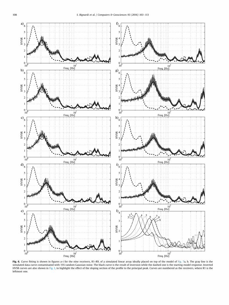
Fig. 6. Curve fitting is shown in figures a–i for the nine receivers, R1–R9, of a simulated linear array ideally placed on top of the model of Fig. 7a, b. The gray line is thesimulated data curve contaminated with 15% random Gaussian noise. The black curve is the result of inversion while the dashed one is the starting model response. InvertedHVSR curves are also shown in Fig. 1, to highlight the effect of the sloping section of the profile to the principal peak. Curves are numbered as the receivers, where R1 is theleftmost one.

S. Bignardi et al. / Computers & Geosciences 93 (2016) 103–113108

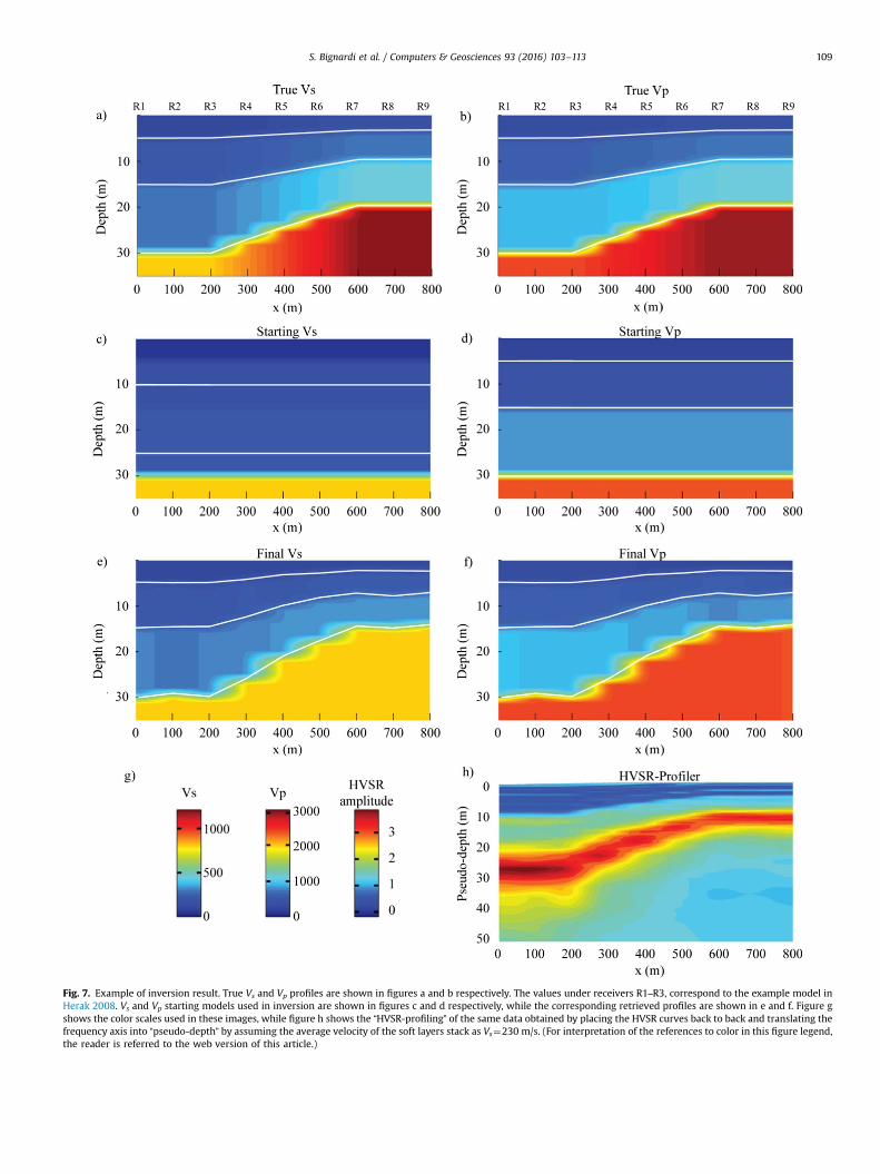
Fig. 7. Example of inversion result. True Vs and Vp profiles are shown in figures a and b respectively. The values under receivers R1–R3, correspond to the example model inHerak 2008. Vs and Vp starting models used in inversion are shown in figures c and d respectively, while the corresponding retrieved profiles are shown in e and f. Figure gshows the color scales used in these images, while figure h shows the “HVSR-profiling” of the same data obtained by placing the HVSR curves back to back and translating thefrequency axis into “pseudo-depth” by assuming the average velocity of the soft layers stack as Vs¼230 m/s. (For interpretation of the references to color in this figure legend,the reader is referred to the web version of this article.)

S. Bignardi et al. / Computers & Geosciences 93 (2016) 103–113 109

S. Bignardi et al. / Computers & Geosciences 93 (2016) 103–113110

parameter m, Eq. (8) before the integration with respect to fre-quency of Eq. (5)

⟦ ⟧⟦ ⟧( )( )

( )

( )= − − − +

∂

∂− ∂

∂−

∂

∂− ∂

∂

( ) ( )

( ) ( )⎛⎝⎜

⎞⎠⎟

⎛⎝⎜

⎞⎠⎟ 8

dE a D D D D

bD

fD

f

D

fD

f

m m m

m m

c f c f c c f best c

c f c c f c

, , , 02

, , 02

, 02

, 02

As stated previously, when a limited portion of the HVSR curveis inverted, the subsurface elastic parameters are randomly per-turbed. When a good match between the data and the simulatedcurve is found, the subsurface model that produced the simulatedcurve is accepted. Unfortunately, if some parameter has a poorinfluence on the shape of the simulated curve and in turn on themisfit (i.e. has a low sensitivity), a good match can be found even ifan improbable value of such a parameter is present. The functiondE(f,m), allows the user to judge which portion of the HVSR curveis affected by a change in a specific parameter. Further, positiveand negative variations of dE(f,m), plotted in red and blue re-spectively, are associated with an increase and decrease of thefrequency dependent contribution to the misfit. By this test, wecan judge how a particular parameter impacts the misfit value,which portion of the HVSR curve is accountable for the change andhow that parameter should be changed in order to decrease themisfit. Furthermore, when unreasonable parameter values arepresent, it can guide the user to find the correction to obtain amore plausible model.

3. Simulated data example

We firstly tested the algorithm on simulated data. To do so, wegenerated nine different HVSR curves along a profile starting fromlocation R1 (x¼0) to location R9 (x¼900) m and spaced at 100 mintervals (Fig. 7). The obtained curves were perturbed with anormally distributed random noise with one sigma correspondingto 15% of perturbation. The noisy curves (a)–(i) in Fig. 6 were thenused as input data for the inversion.

In 2010, Herak showed a successful inversion performed byoptimizing Vs and Vp of the layers while keeping all other para-meters fixed. In this test, we relaxed these constraints allowing forboth velocities (Vs, Vp) and thicknesses (H) to change. The half-space parameters were kept fixed, however, this constrain isknown to have a negligible impact on the inversion. In order toobtain a rough starting model for the laterally constrained opti-mization, we independently optimized the subsurface model un-der each HVSR curve by allowing a 5% perturbation for the first3000 iterations and then successively allowing 15% perturbationfor the next 5000 iterations. In general, a few hundred generationsper location was sufficient to find the best 1D local model; but wedecided to extend the computation up to 8000 random genera-tions to enhance the sampling of the parameter space.

Correspondingly, the true subsurface model is plotted in termsof 2D profiles of Vp and Vs in Fig. 7a and b respectively. The sub-surface under stations R1–R3 is assumed to be the same used byHerak (2008). The thickness regularly decreases between stationsR3 and R7 and then becomes constant under locations R7–R9. Fi-nally, the inversion was performed by starting from the model inFig. 7c and d. Later, in order to obtain the model which best sa-tisfies Eq. (3), we started from the latter rough model, composed ofall the optimal 1D local models and we performed 30,000 per-turbations of the entire profile as a whole, allowing perturbationsof 20% with respect to the best model. The results in the data spaceare shown in Fig. 6a–i, where the best fitting curves (solid black)are compared to the data (solid gray) and to the initial model re-sponse (dashed black). Fig. 6l shows the best curves obtained at

different locations. The best result in the parameter space is shownin term of Vs and Vp profiles (Fig. 7e, f). Further, for sake of com-parison, the result of HVSR-profiling, where the HVSR amplitude isplotted in terms of pseudo-depth is shown in Fig. 7h. To obtain thelatter figure we used, for the frequency-to-depth conversion,Vs¼230 m/s which in this case proved to be the correct value. Itcan be noted that the profiler result is in good accordance with theinversion.

4. Real data case

In this section we present a simplified inversion example ofmultiple HVSR curves collected along a linear profile in the fra-mework of the Italian DPC-INGV Seismological Projects S1 (Abu-Zeid et al., 2014; Mantovani et al., 2015) with the purpose of ac-quiring the deep shear wave velocity (up to 150 m depth) in theProvince of Ferrara, both for microzonation purposes and todocument the occurrence of recent tectonic evolution of the cen-tral-eastern sector of the Po Plain nearby the town. A geophysicalsurvey along two profiles was carried out, ca. 27 km-long almostperpendicular to the regional trend of the underlying tectonicstructures (Fig. 8a, b), based essentially on passive seismicmeasurements.

The measurements were performed using a three-componentshort-period seismometer (fc¼2 Hz) for time intervals of 50 minand HVSR curves were computed using a window size of 60 s.

In Fig. 9 we present a portion of the 2D Vs profile obtained afterinverting the subset of the data highlighted with the green squaresin Fig. 8. Along the investigated area, the pseudo-bedrock (whitedashed line in Fig. 9a) undergoes various depth variations and it isexpected to gently deepen moving from the south to the north(R1–R8 in Fig. 9a). The main frequency peak observed in the PoPlain is well documented to be variable depending on the location(Martelli et al., 2014; Paolucci et al., 2015) with fundamental fre-quency ranging from 0.5 to 1.5 Hz. Considered this, the analysiswas limited in the frequency band between 0.5 and 6 Hz. Theobtained depth of the major impedance contrast is consistent withthose of the other geophysical tests and available informationabout the subsurface stratigraphy. In particular, the pseudo-bed-rock here detected could correspond to the contact between twosedimentary cycles, both belonging to an higher rank sedimentarycycle represented by the Upper Emiliano-Romagnolo Synthem(RER and ENI-AGIP, 1998).

In the following, Fig. 9a shows the Vs profile obtained byOpenHVSR and for sake of comparison Fig. 9b shows the corre-sponding HVSR-profiling. Further, Fig. 10a–h, show the comparisonbetween the data and the theoretical curves in the frequency band0.5–6.0 Hz. Such a result was achieved using a semi-automaticstrategy. We performed three sessions of model improvement,each consisting of separately inverting each curve by allowing a 5%perturbation in the Monte Carlo algorithm and running 5000single-curve random perturbations, followed by 10,000 laterallyconstrained perturbations. We started from a simple 4 layersmodel and whenever necessary, we progressively increased thenumber of layers among sessions. This was possible thanks to theimproved flexibility of the interface which allowed to test thechanges introduced by adding new layers, and allowed to quicklysave and reload the models obtained after each modification. Afourth and final session was performed after the subsurface modelwas considered satisfactory; we increased the amount of pertur-bation up to 20%, allowing 10,000 single-curve perturbations,followed by 10,000 laterally constrained perturbations. The wholeprocess required roughly 3 h on an INTEL I7 (1.8–2.4 GHz), 8 GbRAM computer running Linux.

Fig. 8. (a) Simplified tectonic map of the blind northern Apennines showing the two studied profiles (Pieri and Groppi, 1981). (b) Location of the single-station mea-surements (squares). HVSR measurements used in the example are highlighted in green. (For interpretation of the references to color in this figure legend, the reader isreferred to the web version of this article.)

S. Bignardi et al. / Computers & Geosciences 93 (2016) 103–113 111

5. Conclusions

In this paper, we introduced a novel program developed in theMatlab environment for the simulation and/or inversion of mas-sive HVSR datasets with the goal of constructing a 2D/3D sub-surface in terms of viscoelastic parameters; which to our knowl-edge has no analogue in the literature. The program was designedfor maximum interactivity and dynamicity. The underlying for-ward routine, available in Fortran from Herak (2008) was portedinto Matlab for compatibility with future releases of this platform.The inversion algorithm, based on the guided Monte Carlo meth-od, is fully customizable and it implements many novel featuresnot seen previously. In particular the subsurface model

Fig. 9. Results for the real data case, 8 HVSR curves performed along a profile running ESthe seismic pseudo-bedrock to steeping toward NNE. (b) For sake of comparison, the cocurves back to back and translating the frequency axis into “pseudo-depth” by assumin

perturbation can be set to be depth dependent, relaxation onelastic parameter constraints now allows the user to account forthe water table and finally, the user can, at any time, pause theinversion and manually investigate or modify the subsurfacemodel parameters with the capability of testing the result of sucha change before accepting it. Other than the confidence estimationtools already present in ModelHVSR which were integrated in thepresent code and are now extended to the lateral variation con-fidence evaluation, a novel tool was introduced which allows theuser to investigate how each parameter perturbation impactsdifferent portions of the HVSR curve. Furthermore, two novelterms were introduced in the objective function of the inversionalgorithm. The first is based on matching the slope of the HVSR

E to the city of Ferrara, Italy; (a) The 2-D Vs profile obtained by the inversion showsrresponding image obtained by HVSR-profiling, which consists of placing the HVSRg, for the soft layers Vs¼350 m/s.

Fig. 10. Results of the inversion in the data space; (a)–(h) shows the best match we achieved for the frequency band 0.5–6.0 Hz, corresponding locations over the profile areindicated in Fig. 8 with R1–R8 labels respectively. HVSR's and error bounds are drawn in black and gray respectively, while the best model response is drawn in red. Further,amplification functions for P (PAF) and S (SAF) waves are drawn in cyan and magenta respectively. (For interpretation of the references to color in this figure legend, thereader is referred to the web version of this article.)

S. Bignardi et al. / Computers & Geosciences 93 (2016) 103–113112

curves rather than their amplitudes and allows for better con-straining of the peaks position, especially when inverting lowquality curves. The second term is a regularizing term which canbe used to impose a lateral smoothness condition. Effectiveness ofthe method was successfully shown both on simulated and realdata. The successful results encouraged and motivated us to pub-lish the present code in an open source format.

Acknowledgments

The authors would like to thank the University of Ferrara forsponsoring this research and in particular Prof. Giovanni Santarato,University of Ferrara, for the valuable advice regarding the math-ematical implementation and the optimization of the graphicalinterface and Prof. Anthony Yezzi (Georgia Institute of Technology)for the valuable suggestions during the development of this work.We would like to thank the Lions Club International - District 108Tb, Bologna (Italy) for the support in acquiring of the in-strumentation. Finally, we would like to thank Prof. Marijan Herak(University of Zagreb, Croatia), who first developed and distributedModelHVSR as open source, making an implementation baseavailable for some of the tools integrated into this code.

Appendix A. Supplementary material

Supplementary data associated with this article can be found inthe online version at http://dx.doi.org/10.1016/j.cageo.2016.05.009.

References

Abu-Zeid, N., Bignardi, S., Caputo, R., Mantovani, A., Tarabusi, G., Santarato, G., 2014.Shear-wave velocity profiles across the Ferrara arc: a contribution for assessingthe recent activity of blind tectonic structures. In: Proceedings of the 33thGNGTS National Convention, vol. 1, pp. 117–122.

Aki, K., Richards, P.G., 2002. Quantitative Seismology, second ed., University ScienceBooks, Sausalito, CA, p. 700.

Albarello, D., Cesi, C., Eulilli, V., Lunedei, E., Paolucci, E., Pileggi., D., Puzzilli, L.M.,2011. The contribution of the ambient vibration prospecting in seismic mi-crozoning: an example from the area damaged by the 26th April 2009 l’Aquila(Italy) earthquake. Boll. di. Geofis. Teor. Ed. Appl. 52 (3), 513–538.

Ben-Menahem, A., Singh, S.J., 1981. Seismic Waves and Sources. Springer-Verlag,New York.

Bianco, F., Del Pezzo, E., Castellano, M., Ibanez, J., Di Luccio, F., 2002. Separation ofintrinsic and scattering seismic attenuation in the southern Apennine zone,Italy. Geophys. J. Int. 150, 10–22.

D’Amico, V., Picozzi, M., Baliva, F., Albarello, D., 2008. Ambient noise measurementsfor preliminary site-effects characterization in the urban area of Florence, Italy.Bull. Seismol. Soc. Am. 98, 1373–1388.

Fantoni, R., Franciosi, R., 2008. Geological sections crossing Po Plain and Adriaticforeland. Rend. Online Soc. Geol. Ital. 3 (1), 367–368.

Gallipoli, M.R., Mucciarelli, M., Eeri, M., Gallicchio, S., Tropeano, M., Lizza, C., 2004a.Horizontal to Vertical Spectral Ratio (HVSR) measurements in the area

S. Bignardi et al. / Computers & Geosciences 93 (2016) 103–113 113

damaged by the 2002 Molise, Italy earthquake. Earthq. Spectra 20 (1), 81–93.Gallipoli, M.R., Mucciarelli, M., Castro, R.R., Mochavesi, G., Contri, P., 2004b. Struc-

ture, soil-structure response and effects of damage based on observations ofhorizontal-to-vertical spectral ratios of microtremors. Soil Dyn. Earthq. Eng. 24,487–495.

Herak, M., 2008. ModelHVSR-A Matlab tool to model horizontal-to-vertical spectralratio of ambient noise. Comput. Geosci. 34, 1514–1526.

Herak, M., Allegretti, I., Herak, D., Kuk, K., Kuk, V., Marić, K., Markušić, S., Stipčević,J., 2010. HVSR of ambient noise in Ston (Croatia): comparison with theoreticalspectra and with the damage distribution after the 1996 Ston-Slano earth-quake. Bull. Earthq. Eng. 8, 483–499.

Hinzen, K.G., Scherbaum, F., Weber, B., 2004. On the resolution of H/V measure-ments to determine sediment thickness, a case study across a normal fault inthe Lower Rhine embayment, Germany. J. Earthq. Eng. 8, 909–926.

Kobayashi, K., 1980. A method for presuming deep ground soil structures by meansof longer period microtremors. In: Proceedings of the 7th WCEE, September 8–13, Istanbul, Turkey, vol. 1, pp. 237–240.

Lunedei, E., Albarello, D., 2015. Horizontal-to-vertical spectral ratios from a full-wavefield model of ambient vibrations generated by a distribution of spatiallycorrelated surface sources. Geophys. J. Int. 201 (2), 1140–1153. http://dx.doi.org/10.1093/gji/ggv046.

Lunedei, E., Albarello, D., 2010. Theoretical HVSR curves from full wavefield mod-elling of ambient vibrations in a weakly dissipative layered Earth. Geophys. J.Int. 181, 1093–1108. http://dx.doi.org/10.1111/j.1365-246X.2010.04560.x.

Mantovani, A., Abu-Zeid, N., Bignardi, S., Santarato, G., 2015. A geophysical transectacross the central sector of the Ferrara Arc: passive seismic investigations - partII. In: Proceedings of the 34th GNGTS National Convention, vol. 1, pp. 114–120.

Martelli, L., Severi, P., Biavati, G., Rosselli, S., Camassi, R., Ercolani, E., Marcellini, A.,Tento, A., Gerosa, D., Albarello, D., Guerrini, F., Lunedei, E., Pileggi, D., Pergalani,F., Compagnoni, M., Fioravante, V., Giretti, D., 2014. Analysis of the local seismichazard for the stability tests of the main bank of the Po River (Northern Italy).Boll. di Geofis. Teor. Ed. Appl. 55, 119–134.

Mayeda, K., Koyanagi, S., Hoshiba, M., Aki, K., Zeng, Y., 1992. A comparative study ofscattering, intrinsic, and coda Q̂-1 for Hawaii, long valley and central Californiabetween 1.5 and 15 Hz. J. Geophys. Res. 97, 6643–6659.

Mucciarelli, M., Gallipoli, M.R., 2001. A critical review of 10 years of microtremor

HVSR technique. Boll. di Geofis. Teor. Ed. Appl. 42, 255–266.Nakamura, Y., 1989. A method for dynamic characteristics estimation of subsurface

using microtremor on the ground surface. Q. Report. Railw. Tech. Res. Inst. 30,25–33.

Nakamura, Y., 1996. Real time information systems for seismic hazards mitigationUrEDAS, HERAS and PIC. Q. Report. Railw. Tech. Res. Inst. 37 (3), 112–127.

Nakamura, Y., 2000. Clear identification of fundamental idea of Nakamura's tech-nique and its applications. In: Proceedings of the 12th World Conference onEarthquake Engineering, New Zealand, 8 pp.

Nogoshi, M., Igarashi, T., 1971. On the amplitude characteristics of microtremor(Part 2). J. Seismol. Soc. Jpn. 24, 26–40 (in Japanese).

Paolucci, E., Albarello, D., D’Amico, S., Lunedei, E., Martelli, L., Mucciarelli, M., Pi-leggi, D., 2015. A large scale ambient vibration survey in the area damaged byMay–June 2012 seismic sequence in Emilia Romagna, Italy. Bull. Earthq. Eng. 13,3187–3206.

Parolai, S., Bormann, P., Milkereit, C., 2002. New relationships between vs, thicknessof the sediments and resonance frequency calculated by means of H/V ratio ofseismic noise for the Cologne area (Germany). Bull. Seismol. Soc. Am. 92 (6),2521–2527.

Pieri, M., Groppi, G., 1981. Subsurface geological structure of the Po Plain, Naples,Italy CNR, Prog. Final. Geodin., Pubbl. no. 414.

Sánchez-Sesma, F.J., Rodríguez, M., Iturrarán-Viveros, U., Luzón, F., Campillo, M.,Margerin, L., García-Jerez, A., Suarez, M., Santoyo, M.A., Rodríguez-Castellanos,A., 2011. A theory for microtremor H/V spectral ratio: application for a layeredmedium. Geophys. J. Int. 186, 221–225. http://dx.doi.org/10.1111/j.1365-246X.2011.05064.x.

RER, ENI-AGIP, 1998. Riserve idriche sotterranee della Regione Emila-Romagna. Acura di G. DI DIO. S.EL.CA. (Firenze).

Scherbaum, F., Hinzen, K.G., Ohrnberger, M., 2003. Determination of shallow shearwave velocity profiles in the Cologne/Germany area using ambient vibrations.Geophys. J. Int. 152, 597–612.

Shiono, K., Ohta, Y., Kudo, K., 1979. Observation of 1–5 s microtremors and theirapplications to earthquake engineering, Part VI: existence of Rayleigh compo-nents. J. Seismol. Soc. Jpn. 35, 115–124.

Tsai, N.C., Housner, G.W., 1970. Calculation of surface motions of a layered half-space. Bull. Seismol. Soc. Am. 60, 1625–1651.