OpenFermion: The Electronic Structure Package for Quantum Computers

Jarrod R. McClean,1, ∗ Kevin J. Sung,2 Ian D. Kivlichan,1, 3 Yudong Cao,4, 5 Chengyu Dai,6 E. Schuyler

Fried,4, 7 Craig Gidney,8 Brendan Gimby,2 Pranav Gokhale,9 Thomas Haner,10 Tarini Hardikar,11 Vojtech

Havlıcek,12 Oscar Higgott,13 Cupjin Huang,2 Josh Izaac,14 Zhang Jiang,1, 15 Xinle Liu,16 Sam McArdle,17

Matthew Neeley,8 Thomas O’Brien,18 Bryan O’Gorman,19, 15 Isil Ozfidan,20 Maxwell D. Radin,21 Jhonathan

Romero,4 Nicholas Rubin,7 Nicolas P. D. Sawaya,4 Kanav Setia,11 Sukin Sim,4 Damian S. Steiger,1, 10

Mark Steudtner,18, 22 Qiming Sun,23 Wei Sun,16 Daochen Wang,24 Fang Zhang,2 and Ryan Babbush1, †

1Google Inc., Venice, CA 902912Department of Electrical Engineering and Computer Science, University of Michigan, Ann Arbor, MI 48109

3Department of Physics, Harvard University, Cambridge, MA 021384Department of Chemistry and Chemical Biology, Harvard University, Cambridge, MA 02138

5Zapata Computing Inc., Cambridge 021386Department of Physics, University of Michigan, Ann Arbor, MI 48109

7Rigetti Computing, Berkeley CA 947108Google Inc., Santa Barbara, CA 93117

9Department of Computer Science, University of Chicago, Chicago, IL 6063710Theoretische Physik, ETH Zurich, 8093 Zurich, Switzerland

11Department of Physics, Dartmouth College, Hanover, NH 0375512Department of Computer Science, Oxford University, Oxford OX1 3QD, United Kingdom

13Department of Physics and Astronomy, University College London,Gower Street, London WC1E 6BT, United Kingdom

14Xanadu, 372 Richmond St W, Toronto, M5V 1X6, Canada15QuAIL, NASA Ames Research Center, Moffett Field, CA 94035

16Google Inc., Mountain View, CA 9404317Department of Materials, University of Oxford,Parks Road, Oxford OX1 3PH, United Kingdom

18Instituut-Lorentz, Universiteit Leiden, 2300 RA Leiden, The Netherlands19BQIC, University of California, Berkeley, CA 94720

20D-Wave Systems Inc., Burnaby, BC21Materials Department, University of California Santa Barbara, Santa Barbara, CA 9310622QuTech, Delft University of Technology, Lorentzweg 1, 2628 CJ Delft, The Netherlands

23Division of Chemistry and Chemical Engineering,California Institute of Technology, Pasadena, CA 91125

24Joint Center for Quantum Information and Computer Science,University of Maryland, College Park, MD 20742

(Dated: February 28, 2019)

Quantum simulation of chemistry and materials is predicted to be an important application forboth near-term and fault-tolerant quantum devices. However, at present, developing and studyingalgorithms for these problems can be difficult due to the prohibitive amount of domain knowl-edge required in both the area of chemistry and quantum algorithms. To help bridge this gapand open the field to more researchers, we have developed the OpenFermion software package(www.openfermion.org). OpenFermion is an open-source software library written largely in Pythonunder an Apache 2.0 license, aimed at enabling the simulation of fermionic and bosonic modelsand quantum chemistry problems on quantum hardware. Beginning with an interface to commonelectronic structure packages, it simplifies the translation between a molecular specification and aquantum circuit for solving or studying the electronic structure problem on a quantum computer,minimizing the amount of domain expertise required to enter the field. The package is designed tobe extensible and robust, maintaining high software standards in documentation and testing. Thisrelease paper outlines the key motivations behind design choices in OpenFermion and discusses somebasic OpenFermion functionality which we believe will aid the community in the development ofbetter quantum algorithms and tools for this exciting area of research.

∗ Corresponding author: jarrodmcc@gmail.com† Corresponding author: ryanbabbush@gmail.com

arX

iv:1

710.

0762

9v5

[qu

ant-

ph]

27

Feb

2019

2

INTRODUCTION

Recent strides in the development of hardware for quantum computing demand comparable developments in theapplications and software these devices will run. Since the inception of quantum computation, a number of promisingapplication areas have been identified, ranging from factoring [1] and solutions of linear equations [2] to simulationof complex quantum materials. However, while the theory has been well developed for many of these problems, thechallenge of compiling efficient algorithms for these devices down to hardware realizable gates remains a formidableone. While this problem is difficult to tackle in full generality, significant progress can be made in particular areas.Here, we focus on what was perhaps the original application for quantum devices, quantum simulation.

Beginning with Feynman in 1982 [3], it was proposed that highly controllable quantum devices, later to becomeknown as quantum computers, would be especially good at the simulation of other quantum systems. This notionwas later formalized to show how in particular instances, we expect an exponential speedup in the solution of theSchrodinger equation for chemical systems [4–9]. This opens the possibility of understanding and designing newmaterials, drugs, and catalysts that were previously untenable. There has also been substantial work applying thesemethods to other fermionic systems such as the Hubbard model [10–12] and Sachdev-Ye-Kitaev model [13, 14]. Sincethe initial work in this area, there has been great progress developing new algorithms [15–30], tighter bounds andbetter implementation strategies [27, 28, 31–37], more desirable Hamiltonian representations [38–50], fault-tolerantresource estimates and layouts [51–53], and proof-of-concept experimental demonstrations [54–57]. Moreover, withmounting experimental evidence, variational and hybrid-quantum classical algorithms [58–69] for these systems havebeen identified as particularly promising approaches when one has limited resources; some speculate these quantumalgorithms may even solve classically intractable instances without error-correction.

However, despite immense progress, much work is left to be done in optimizing algorithms in this area for bothnear-term and far-future devices. Already this field has seen instances where the difference between naive boundsfor algorithms and expected numerics for real systems can differ by many orders of magnitude [19, 34–36, 52].Unfortunately, developing algorithms in this area can require a prohibitive amount of domain expertise. For example,quantum algorithms experts may find the chemistry literature rife with jargon and unknown approximations whilechemists find themselves unfamiliar with the concepts used in quantum information. As has been seen though, bothhave a crucial role to play in developing algorithms for these emerging devices.

For this reason, we introduce the OpenFermion package, designed to bridge the gap between different domainareas and facilitate the development of explicit quantum simulation algorithms for quantum chemistry. The goalof this project is to enable both quantum algorithm developers and quantum chemists to make contributions tothis developing field, minimizing the amount of domain knowledge required to get started, and aiding those withknowledge to perform their work more quickly and easily. OpenFermion is an open-source Apache 2.0 licensedsoftware package to encourage community adoption and contribution. It has a modular design and is maintainedwith strict documentation and testing standards to ensure robust code and project longevity. Moreover, to maximizeusefulness within the field, every effort has been made to design OpenFermion as a modular library which is agnosticwith respect to quantum programming language frameworks. Through its plugin system, OpenFermion is able tointerface with, and benefit from, any of the frameworks being developed for both more abstract quantum softwareand hardware specific compilation [70–80].

This technical document introduces the first release of the OpenFermion package and proceeds in the following way.We begin by mapping the standard workflow of a researcher looking to implement an electronic structure problem ona quantum computer, giving examples along this path of how OpenFermion aids the researcher in making this processas painless as possible. We aim to make this exposition accessible to all interested readers, so some background inthe problem is provided as well. The discussion then shifts to the core and derived data structures the package isdesigned around. Following this, some example applications from real research projects are discussed, demonstratingreal-world examples of how OpenFermion can streamline the research process in this area. Finally, we finish with abrief discussion of the open source philosophy of the project and plans for future developments.

I. QUANTUM WORKFLOW PIPELINE

In this section we step through one of the primary problems in entering quantum chemistry problems to a quantumcomputer. Specifically, the workflow for translating a problem in quantum chemistry to one in quantum computing.This process begins by specifying the problem of interest, which is typically finding some molecular property for aparticular state of a molecule or material. This requires one to specify the molecule of interest, usually through thepositions of the atoms and their identities. However, this problem is also steeped in some domain specific terminology,especially with regards to symmetries and choices of discretizations. OpenFermion helps to remove many of theseparticular difficulties. Once the problem has been specified, several computational intermediates must be computed,

3

namely the bare two-electron integrals in the chosen discretization as well as the transformation to a molecular orbitalbasis that may be needed for certain correlated methods. From there, translation to qubits may be performed by oneof several mappings. The goal of this section is to both detail this pipeline, and show at each step how OpenFermionmay be used to help perform it with ease.

A. Molecule specification and input generation

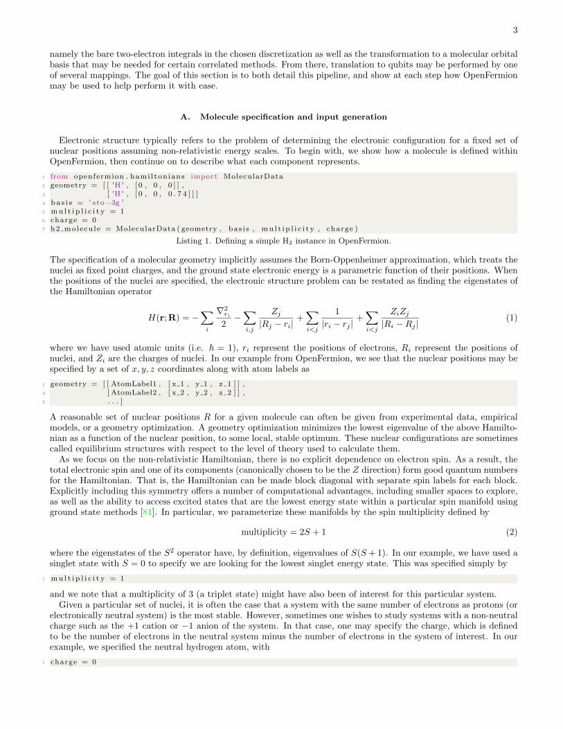
Electronic structure typically refers to the problem of determining the electronic configuration for a fixed set ofnuclear positions assuming non-relativistic energy scales. To begin with, we show how a molecule is defined withinOpenFermion, then continue on to describe what each component represents.

1 from openfermion . hami l ton ians import MolecularData2 geometry = [ [ 'H ' , [ 0 , 0 , 0 ] ] ,3 [ 'H ' , [ 0 , 0 , 0 . 7 4 ] ] ]4 ba s i s = ' sto−3g '5 mu l t i p l i c i t y = 16 charge = 07 h2 molecu le = MolecularData ( geometry , bas i s , mu l t i p l i c i t y , charge )

Listing 1. Defining a simple H2 instance in OpenFermion.

The specification of a molecular geometry implicitly assumes the Born-Oppenheimer approximation, which treats thenuclei as fixed point charges, and the ground state electronic energy is a parametric function of their positions. Whenthe positions of the nuclei are specified, the electronic structure problem can be restated as finding the eigenstates ofthe Hamiltonian operator

H(r;R) = −∑i

∇2ri

2−∑i,j

Zj|Rj − ri|

+∑i<j

1

|ri − rj |+∑i<j

ZiZj|Ri −Rj |

(1)

where we have used atomic units (i.e. ~ = 1), ri represent the positions of electrons, Ri represent the positions ofnuclei, and Zi are the charges of nuclei. In our example from OpenFermion, we see that the nuclear positions may bespecified by a set of x, y, z coordinates along with atom labels as

1 geometry = [ [ AtomLabel1 , [ x 1 , y 1 , z 1 ] ] ,2 [ AtomLabel2 , [ x 2 , y 2 , z 2 ] ] ,3 . . . ]

A reasonable set of nuclear positions R for a given molecule can often be given from experimental data, empiricalmodels, or a geometry optimization. A geometry optimization minimizes the lowest eigenvalue of the above Hamilto-nian as a function of the nuclear position, to some local, stable optimum. These nuclear configurations are sometimescalled equilibrium structures with respect to the level of theory used to calculate them.

As we focus on the non-relativistic Hamiltonian, there is no explicit dependence on electron spin. As a result, thetotal electronic spin and one of its components (canonically chosen to be the Z direction) form good quantum numbersfor the Hamiltonian. That is, the Hamiltonian can be made block diagonal with separate spin labels for each block.Explicitly including this symmetry offers a number of computational advantages, including smaller spaces to explore,as well as the ability to access excited states that are the lowest energy state within a particular spin manifold usingground state methods [81]. In particular, we parameterize these manifolds by the spin multiplicity defined by

multiplicity = 2S + 1 (2)

where the eigenstates of the S2 operator have, by definition, eigenvalues of S(S + 1). In our example, we have used asinglet state with S = 0 to specify we are looking for the lowest singlet energy state. This was specified simply by

1 mu l t i p l i c i t y = 1

and we note that a multiplicity of 3 (a triplet state) might have also been of interest for this particular system.Given a particular set of nuclei, it is often the case that a system with the same number of electrons as protons (or

electronically neutral system) is the most stable. However, sometimes one wishes to study systems with a non-neutralcharge such as the +1 cation or −1 anion of the system. In that case, one may specify the charge, which is definedto be the number of electrons in the neutral system minus the number of electrons in the system of interest. In ourexample, we specified the neutral hydrogen atom, with

1 charge = 0

4

Finally, to specify the computational problem to be solved, rather than simply the molecule itself, it is necessary todefine the basis set. This is analogous to, in some loose sense, how one might define a grid to solve a a simple partialdifferential equation such as the heat-equation. In chemistry, much thought has gone into optimizing specialized basissets to pack the essential physics of the problems into functions that balance cost and accuracy. A list of some ofthe most common basis sets expressed as sums of Gaussians can be found in the EMSL basis set exchange [82]. Inthis case, we specify the so-called minimal basis set “sto-3g”, which stands for 3 Gaussians (3G) used to approximateSlater-type orbitals (STO). This is done through the line

1 ba s i s = ' sto−3g '

In future implementations, the code may additionally support parametric or user defined basis sets with similar syntax.At present, the code supports basis sets that are implemented within common molecular electronic structure packagesthat will be described in more detail in the next section. With the above specifications, the chemical problem is nowwell defined; however, several steps remain in mapping to a qubit representation.

B. Integral generation

After the specification of the molecule as in the previous section, it becomes necessary to do some of the numericalwork in generating the problem to be solved. In OpenFermion we accomplish this through plugin libraries that inter-face with existing electronic structure codes. At present there are supported interfaces to Psi4 [83] and PySCF [84],with plans to expand to other common packages in the future. One needs to install these plugin libraries separatelyfrom the core OpenFermion library (instructions are provided at www.openfermion.org that includes a Docker alter-native installing all these packages). We made the decision to support these packages as plugins rather than directlyintegrating them for several reasons. First, some of these packages have different open source licenses than Open-Fermion. Second, these packages may require more intricate installations and do not run on all operating systems.Finally, in the future one may wish to use OpenFermion in conjunction with other electronic structure packages whichmight support methods not implemented in Psi4 and PySCF. The plugin model ensures the modularity necessary tomaintain such compatibilities as the code evolves.

Once one has chosen a particular basis and enforced the physical anti-symmetry of electrons, the electronic structureproblem may be written exactly in the form of a second quantized electronic Hamiltonian as

H(R) =∑ij

hij(R)a†iaj +1

2

∑ijkl

hijkl(R)a†ia†jakal. (3)

The coefficients hij and hijkl are defined by the basis set that was chosen for the problem (sto-3g in our example);however the computation of these coefficients in general can be quite involved. In particular, in many cases it makessense to perform a Hartree-Fock calculation first and transform the above integrals into the molecular orbital basisthat results. This has the advantage of making the mean-field state easy to represent on both a classical and quantumcomputer, but introduces some challenges with regards to cost of the integral transformation and convergence ofthe Hartree-Fock calculation for challenging systems. For example, it is necessary to specify an initial guess for theorbitals of Hartree-Fock, the method used to solve the equations, and a number of other numerical parameters thataffect convergence.

In OpenFermion we address this problem by choosing a reasonable set of default parameters and interfacing withwell developed electronic structure packages through a set of plugin libraries to supply the information desired. Forexample, using the OpenFermion-Psi4 plugin, one can obtain the two-electron integrals hijkl for this molecule in theMO basis in the Psi4 electronic structure code by simply executing

1 from openfermionps i4 import run ps i 42

3 h2 molecu le = run ps i 4 ( h2 molecule ,4 run mp2=True ,5 run c i sd=True ,6 run ccsd=True ,7 r u n f c i=True )8 tw o e l e c t r o n i n t e g r a l s = h2 molecu le . two body in t eg ra l s

where the h2 molecule is that defined in the previous section and when run in this way, one may easily access the MP2,CISD, CCSD, and FCI energies. This will return the computed two-electron integrals in the Hartree-Fock molecularorbital basis. Moreover, one has direct access to other common properties such as the molecular orbital coefficientsthrough simple commands such as

1 o r b i t a l s = h2 molecu le . c a n o n i c a l o r b i t a l s

5

One may also read the 1- and 2-electron reduced density matrices from CISD and FCI and the converged coupledcluster amplitudes from CCSD. These values are all conveniently stored to disk using an HDF5 interface that onlyloads the properties of interest from disk for convenient analysis of data after the fact.

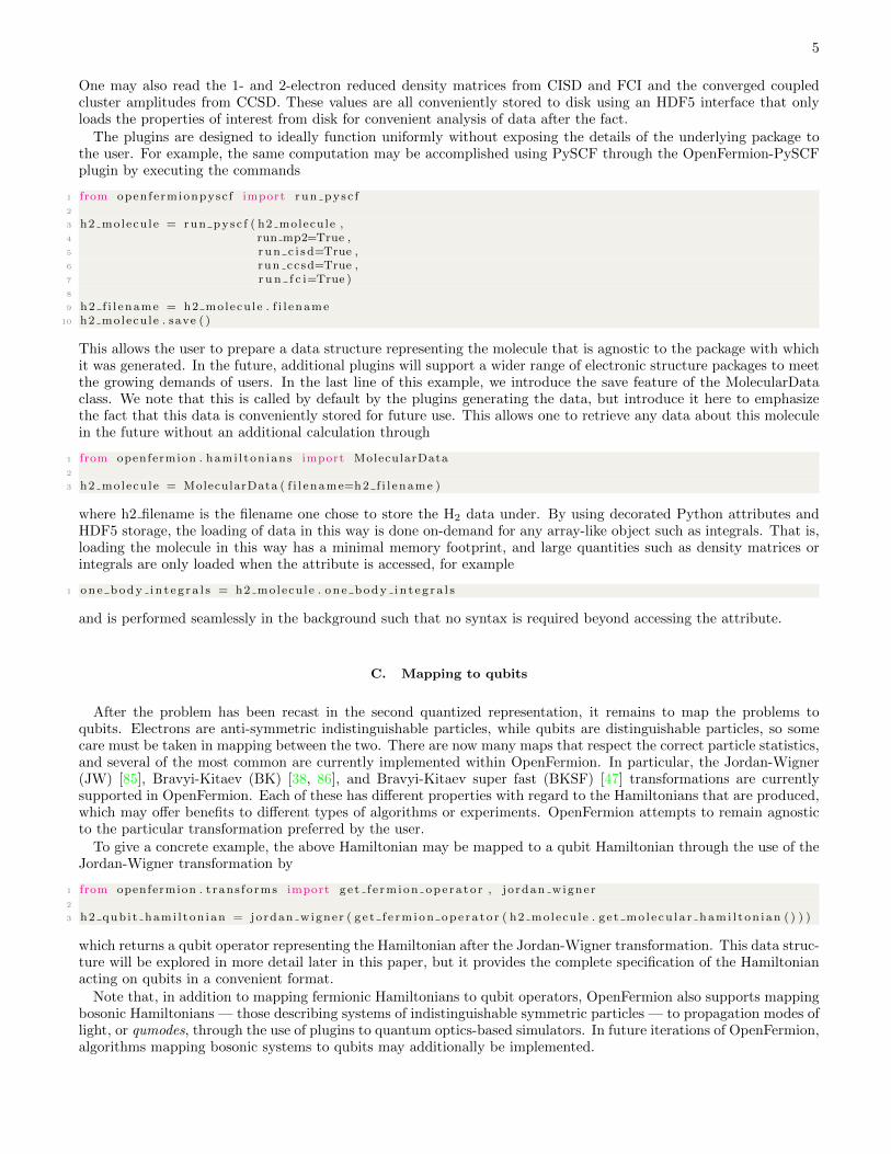
The plugins are designed to ideally function uniformly without exposing the details of the underlying package tothe user. For example, the same computation may be accomplished using PySCF through the OpenFermion-PySCFplugin by executing the commands

1 from openfermionpysc f import run pysc f2

3 h2 molecu le = run pysc f ( h2 molecule ,4 run mp2=True ,5 run c i sd=True ,6 run ccsd=True ,7 r u n f c i=True )8

9 h2 f i l ename = h2 molecu le . f i l ename10 h2 molecu le . save ( )

This allows the user to prepare a data structure representing the molecule that is agnostic to the package with whichit was generated. In the future, additional plugins will support a wider range of electronic structure packages to meetthe growing demands of users. In the last line of this example, we introduce the save feature of the MolecularDataclass. We note that this is called by default by the plugins generating the data, but introduce it here to emphasizethe fact that this data is conveniently stored for future use. This allows one to retrieve any data about this moleculein the future without an additional calculation through

1 from openfermion . hami l ton ians import MolecularData2

3 h2 molecu le = MolecularData ( f i l ename=h2 f i l ename )

where h2 filename is the filename one chose to store the H2 data under. By using decorated Python attributes andHDF5 storage, the loading of data in this way is done on-demand for any array-like object such as integrals. That is,loading the molecule in this way has a minimal memory footprint, and large quantities such as density matrices orintegrals are only loaded when the attribute is accessed, for example

1 one body in t e g r a l s = h2 molecu le . on e body in t e g r a l s

and is performed seamlessly in the background such that no syntax is required beyond accessing the attribute.

C. Mapping to qubits

After the problem has been recast in the second quantized representation, it remains to map the problems toqubits. Electrons are anti-symmetric indistinguishable particles, while qubits are distinguishable particles, so somecare must be taken in mapping between the two. There are now many maps that respect the correct particle statistics,and several of the most common are currently implemented within OpenFermion. In particular, the Jordan-Wigner(JW) [85], Bravyi-Kitaev (BK) [38, 86], and Bravyi-Kitaev super fast (BKSF) [47] transformations are currentlysupported in OpenFermion. Each of these has different properties with regard to the Hamiltonians that are produced,which may offer benefits to different types of algorithms or experiments. OpenFermion attempts to remain agnosticto the particular transformation preferred by the user.

To give a concrete example, the above Hamiltonian may be mapped to a qubit Hamiltonian through the use of theJordan-Wigner transformation by

1 from openfermion . t rans forms import ge t f e rm ion ope ra to r , jo rdan wigner2

3 h2 qub i t hami l ton ian = jordan wigner ( g e t f e rm ion ope r a t o r ( h2 molecu le . g e t mo l e cu l a r hami l t on i an ( ) ) )

which returns a qubit operator representing the Hamiltonian after the Jordan-Wigner transformation. This data struc-ture will be explored in more detail later in this paper, but it provides the complete specification of the Hamiltonianacting on qubits in a convenient format.

Note that, in addition to mapping fermionic Hamiltonians to qubit operators, OpenFermion also supports mappingbosonic Hamiltonians — those describing systems of indistinguishable symmetric particles — to propagation modes oflight, or qumodes, through the use of plugins to quantum optics-based simulators. In future iterations of OpenFermion,algorithms mapping bosonic systems to qubits may additionally be implemented.

6

D. Numerical testing

While the core functionality of OpenFermion is designed to provide a map between the space of electronic structureproblems and qubit-based quantum computers, some functionality is provided for numerical simulation. This can behelpful for debugging or prototyping new algorithms. For example, one could check the spectrum of the above qubitHamiltonian after the Jordan-Wigner transformation by performing

1 from openfermion . t rans forms import g e t s p a r s e op e r a t o r2 from sc ipy . l i n a l g import e igh3

4 h2 matrix = ge t s p a r s e op e r a t o r ( h2 qub i t hami l ton ian ) . todense ( )5 e igenva lue s , e i g env e c t o r s = e igh ( h2 matrix )

which yields the exact eigenvalues and eigenvectors of the H2 Hamiltonian in the computational basis.

E. Compiling circuits for quantum algorithms

The core of OpenFermion consists of tools for obtaining and manipulating representations of quantum operators.These tools and representations are useful for compiling quantum circuits, but the best way to perform this compilationdepends on the particular algorithm and hardware used. Many groups have their own software for performing thiscompilation. OpenFermion is intended to be agnostic with respect to the particular hardware and compilationplatform; we delegate the final compilation step to platform-specific plugins. At the time of writing, plugins aresupported for the Cirq, Forest, and Strawberry Fields [80] frameworks. These plugins are called OpenFermion-Cirq,Forest-OpenFermion, and SFOpenBoson, respectively. Below, we provide examples of using these plugins to compilequantum circuits.

1. OpenFermion-Cirq Example

In our first example, we assume the user has a hydrogen molecule object stored in the variable h2 molecule and useCirq and OpenFermion-Cirq to construct a circuit that simulates time evolution by the molecular Hamiltonian via aproduct formula implemented with the “low rank” strategy described in [49]. We’ll compile just one Trotter step andperform a circuit optimization which merges single-qubit rotations before displaying the circuit.

1 import c i r q2 import open fe rmionc i rq as o f c3

4 hami ltonian = h2 molecu le . g e t mo l e cu l a r hami l t on i an ( )5 qub i t s = c i r q . LineQubit . range (4 )6 c i r c u i t = c i r q . C i r cu i t . f rom ops (7 o f c . s imu l a t e t r o t t e r (8 qubits ,9 hamiltonian ,

10 time=1.0 ,11 n s t ep s =1,12 order=0,13 a lgor i thm=o f c . t r o t t e r .LOWRANK,14 omi t f i na l swap s=True15 )16 )17 c i r q . me r g e s i n g l e qub i t g a t e s i n t o pha s ed x z ( c i r c u i t )18

19 pr in t ( c i r c u i t . t o t ext d iag ram ( u s e un i c od e cha r a c t e r s=Fal se ) )

Executing this code produces an ASCII circuit diagram which we truncate and display below:

0: ---Z^0.535-------------------YXXY--------------------@----------swap--------------------------

| | |

1: ---Z^0.535-----------YXXY----#2^-1-----------YXXY----@^-0.218---swap--------------@-----------

| | | ...

2: ---Z^0.291-----------#2^-1-----------YXXY----#2^-1--------------@----------swap---@^(-3/14)---

| | |

3: ---Z^0.291---------------------------#2^-1----------------------@^-0.211---swap---------------

7

In our next example, we construct a circuit which prepares the ground state of the tunneling term of a Fermi-Hubbard model Hamiltonian. The Fermi-Hubbard model has the Hamiltonian

−t∑〈i,j〉,σ

(a†i,σaj,σ + a†j,σai,σ) + U∑i

a†i,↑ai,↑a†i,↓ai,↓

which is composed of a tunneling term (on the left) and an interaction term (on the right). The tunneling termis a quadratic Hamiltonian and its ground state is a Slater determinant. More generally, eigenstates of quadraticHamiltonians are known as fermionic Gaussian states.

1 import c i r q2 import openfermion3 import open fe rmionc i rq as o f c4

5 hubbard model = openfermion . fermi hubbard (2 , 2 , 1 . 0 , 4 . 0 )6 quad ham = openfermion . g e t quad ra t i c hami l t on i an ( hubbard model , i gno r e in compat ib l e t e rms=True )7

8 qub i t s = c i r q . LineQubit . range (8 )9 c i r c u i t = c i r q . C i r cu i t . f rom ops (

10 o f c . p r epa r e g au s s i a n s t a t e ( qubits , quad ham)11 )12

13 pr in t ( c i r c u i t . t o t ext d iag ram ( t ranspose=True , u s e un i c od e cha r a c t e r s=Fal se ) )

Executing this code produces the following ASCII circuit diagram:

0 1 2 3 4 5 6 7

| | | | | | | |

X X X X | | | |

| | | | | | | |

| | | YXXY------#2^0.859 | | |

| | | | | | | |

| | YXXY------#2^-0.701 Z^0 | | |

| | | | | | | |

| YXXY-----#2^-0.89 Z^0 YXXY-------#2^0.805 | |

| | | | | | | |

YXXY-#2^0.844 Z^0 YXXY------#2^-0.859 Z^0 | |

| | | | | | | |

| Z^0 YXXY------#2^0.607 Z^0 YXXY-----#2^0.844 |

| | | | | | | |

| YXXY-----#2^-0.569 Z^0 YXXY-------#2^0.565 Z^0 |

| | | | | | | |

| | Z^0 YXXY------#2^(13/15) Z^0 YXXY------#2^0.675

| | | | | | | |

| | YXXY------#2^-0.853 Z^0 YXXY-----#2^-0.565 Z^0

| | | | | | | |

| | | Z^0 YXXY-------#2^0.893 Z^0 |

| | | | | | | |

| | | YXXY------#2^0.381 Z^0 | |

| | | | | | | |

| | | | Z^0 | | |

| | | | | | | |

2. Forest-OpenFermion Example

In this section we describe the interface between OpenFermion and Rigetti’s quantum simulation environment calledForest. The interface provides a method of transforming data generated in OpenFermion to a similar representationin pyQuil. For this example we use OpenFermion to build a four-site single-band periodic boundary Hubbard modeland apply first-order Trotter time-evolution to a starting state of two localized electrons of opposite spin.

The Forest-OpenFermion plugin provides the routines to inter-convert between the OpenFermion QubitOperatordata structure and the synonymous data structure in pyQuil called a PauliSum.

1 from openfermion . ops import QubitOperator2 from fo r e s topen f e rmion import pyqu i l pau l i t o qub i t op , qub i t op t o pyqu i l p au l i

8

The FermionOperator in OpenFermion can be used to translate the mathematical expression of the Hamiltonian di-rectly to executable code. While we show how this model can be built in one line using the OpenFermion hamiltoniansmodule below, here we take the opportunity to demonstrate the ease of creating such models for study that could beeasily modified as desired. Given the Hamiltonian of the Hubbard system

H = −1∑〈i,j〉,σ

(a†i,σaj,σ + a†j,σai

)+ 4

3∑i=0

a†i,αai,αa†i,βai,β (4)

where 〈·, ·〉 indicates nearest-neighbor spatial lattice positions and σ takes on values of α and β signifying spin-up orspin-down, respectively, the code to build this Hamiltonian is as follows:

1 from openfermion . t rans forms import jo rdan wigner2 from openfermion . ops import FermionOperator , he rmi t ian con jugated3

4 hubbard hamiltonian = FermionOperator ( )5 s p a t i a l o r b i t a l s = 46 f o r i in range ( s p a t i a l o r b i t a l s ) :7 e l e c t r on hop a lpha = FermionOperator ( ( ( 2 ∗ i , 1) , (2 ∗ ( ( i + 1) % s p a t i a l o r b i t a l s ) , 0) ) )8 e l e c t r on hop be ta = FermionOperator ( ( ( 2 ∗ i + 1 , 1) , ( (2 ∗ ( ( i + 1) % s p a t i a l o r b i t a l s ) + 1) ,

0) ) )9 hubbard hamiltonian += −1 ∗ ( e l e c t r on hop a lpha + hermit ian con jugated ( e l e c t r on hop a lpha ) )

10 hubbard hamiltonian += −1 ∗ ( e l e c t r on hop be ta + hermit ian con jugated ( e l e c t r on hop be ta ) )11 hubbard hamiltonian += FermionOperator ( ( ( 2 ∗ i , 1) , (2 ∗ i , 0) ,12 (2 ∗ i + 1 , 1) , (2 ∗ i + 1 , 0) ) , 4 . 0 )

In the above code we have implicitly used even indexes [0, 2, 4, 6] as α spin-orbitals and odd indexes [1, 3, 5, 7] as βspin-orbitals. The same model can be built using the OpenFermion Hubbard model builder routine in the hamiltoniansmodule with a single function call.

1 from openfermion . hami l ton ians import fermi hubbard2

3 x dim = 44 y dim = 15 p e r i o d i c = True6 ch em i c a l p o t en t i a l = 07 tunne l ing = 1 .08 coulomb = 4.09 o f hubbard hami l ton ian = fermi hubbard ( x dim , y dim , tunne l ing , coulomb ,

10 ch em i c a l p o t en t i a l=None ,11 s p i n l e s s=Fal se )

Using the Jordan-Wigner transform functionality of OpenFermion, the Hubbard Hamiltonian can be transformedto a sum of QubitOperators which are then transformed to pyQuil PauliSum objects using routines in the Forest-OpenFermion plugin imported earlier.

1 hubbard term generator = jordan wigner ( hubbard hamiltonian )2 pyqu i l hubbard generator = qub i t op t o pyqu i l p au l i ( hubbard term generator )

With the data successfully transformed to a pyQuil representation, the pyQuil exponentiate routine is used to generatea circuit corresponding to first-order Trotter evolution for t = 0.1.

1 from pyqu i l . q u i l import Program2 from pyqu i l . ga te s import X3 from pyqu i l . p au l i s import exponent ia te4 l o c a l i z e d e l e c t r o n s p r o g r am = Program ( )5 l o c a l i z e d e l e c t r o n s p r o g r am . i n s t ( [X(0 ) , X(1) ] )6 pyqui l program = Program ( )7 f o r term in pyqu i l hubbard generator . terms :8 pyqui l program += exponent ia te ( 0 . 1 ∗ term )9 pr in t ( l o c a l i z e d e l e c t r o n s p r o g r am + pyqui l program )

1 Sample Output :2 X 03 X 14 X 05 PHASE(−0.4) 06 X 07 PHASE(−0.4) 08 H 0

9

9 H 210 CNOT 0 111 CNOT 1 212 RZ(−0.1) 213 CNOT 1 214 CNOT 0 115 . . .

The output is the first few lines of the Quil [72] program that sets up the two-localized electrons on the first spatial siteand then applies the time-propagation circuit. This Quil program can be sent to the Forest cloud API for simulationor for execution on hardware.

3. SFOpenBoson Example

Quantum optics and continuous-variable (CV) quantum computation provide a well-suited environment for thequantum simulation of bosons. In this example, we describe the interface between OpenFermion and Xanadu’squantum optics-based simulation environment Strawberry Fields, and simulate a Bose-Hubbard model using the CVgate set and propagation modes of light.

Consider the following Bose-Hubbard Hamiltonian, describing bosons on a lattice with on-site interaction strengthU = 1.5 and chemical potential µ = 0.5:

H = −∑〈i,j〉

b†i bj+1 +1.5

2

N−1∑k=1

b†kbk(b†kbk − 1)− 0.5

N∑k=1

b†kbk. (5)

Here, b†i and bi are the bosonic creation and annhilation operators respectively acting on qumode i. Using Open-Fermion, it is a one line procedure to generate this Hamiltonian for a 2× 2 lattice:

1 from openfermion . hami l ton ians import bose hubbard2 H = bose hubbard (2 , 2 , tunne l ing=1, i n t e r a c t i o n =1.5 , c h em i c a l p o t en t i a l =0.5)

We can now use the SFOpenBoson plugin to simulate this Hamiltonian in Strawberry Fields. The SFOpenBosonplugin provides operations to convert the OpenFermion BosonOperator/QuadOperator data structure to the standardoperations and gates used in continuous-variable quantum computation. Using the Hamiltonian defined above, wecan do this as follows:

1 import s t r awb e r r y f i e l d s as s f2 from s t r awb e r r y f i e l d s . ops import Fock3 from sfopenboson . ops import BoseHubbardPropagation4

5 t = 0 .16 eng , q = s f . Engine (4 )7 with eng :8 Fock (2) | q [ 0 ]9 BoseHubbardPropagation (H, t , k=20) | q

In the above code, we create a two qumode quantum circuit with the system initialized in Fock state |2, 0, 0, 0〉, andthen perform the time evolution for t = 0.1 using the Lie product formula truncated to 20 terms. Finally, we run thecircuit simulation, and print the applied quantum gates:

1 s t a t e = eng . run ( ’ fock ’ , cu to f f d im=3)2 eng . p r i n t app l i e d ( )

1 BSgate (−0.005 , 1 . 571 ) | ( q [ 0 ] , q [ 1 ] ) # Beamspl i t te r2 BSgate (−0.005 , 1 . 571 ) | ( q [ 0 ] , q [ 2 ] ) # Beamspl i t te r3 BSgate (−0.005 , 1 . 571 ) | ( q [ 1 ] , q [ 3 ] ) # Beamspl i t te r4 BSgate (−0.005 , 1 . 571 ) | ( q [ 2 ] , q [ 3 ] ) # Beamspl i t te r5 Kgate (−0.00375) | ( q [ 0 ] ) # Kerr i n t e r a c t i o n6 . . .

The output above lists the first few gates applied, and the corresponding qumodes they act on, for the Bose-Hubbardsimulation.

10

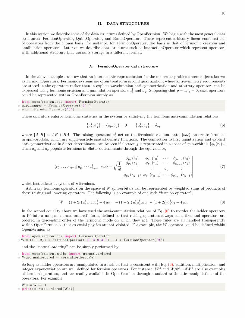
II. DATA STRUCTURES

In this section we describe some of the data structures defined by OpenFermion. We begin with the most general datastructures: FermionOperator, QubitOperator, and BosonOperator. These represent arbitrary linear combinationsof operators from the chosen basis; for instance, for FermionOperator, the basis is that of fermionic creation andannihilation operators. Later on we describe data structures such as InteractionOperator which represent operatorswith additional structure that warrants storage in a different format.

A. FermionOperator data structure

In the above examples, we saw that an intermediate representation for the molecular problems were objects knownas FermionOperators. Fermionic systems are often treated in second quantization, where anti-symmetry requirementsare stored in the operators rather than in explicit wavefunction anti-symmetrization and arbitrary operators can beexpressed using fermionic creation and annihilation operators a†p and aq. Supposing that p = 1, q = 0, such operatorscould be represented within OpenFermion simply as

1 from openfermion . ops import FermionOperator2 a p dagger = FermionOperator ( ' 1ˆ ' )3 a q = FermionOperator ( ' 0 ' )

These operators enforce fermionic statistics in the system by satisfying the fermionic anti-commutation relations,a†p, a

†q

= ap, aq = 0

a†p, aq

= δpq. (6)

where A,B ≡ AB + BA. The raising operators a†p act on the fermionic vacuum state, |vac〉, to create fermionsin spin-orbitals, which are single-particle spatial density functions. The connection to first quantization and explicitanti-symmetrization in Slater determinants can be seen if electron j is represented in a space of spin-orbitals φp(rj).Then a†p and ap populate fermions in Slater determinants through the equivalence,

〈r0, . . . , rη−1| a†p0 · · · a†pη−1|vac〉 =

√1

η!

∣∣∣∣∣∣∣∣∣φp0 (r0) φp1 (r0) · · · φpη−1 (r0)φp0 (r1) φp1 (r1) · · · φpη−1 (r1)

......

. . ....

φp0 (rη−1) φp1 (rη−1) · · · φpη−1(rη−1)

∣∣∣∣∣∣∣∣∣ (7)

which instantiates a system of η fermions.Arbitrary fermionic operators on the space of N spin-orbitals can be represented by weighted sums of products of

these raising and lowering operators. The following is an example of one such “fermion operator”,

W = (1 + 2i) a†4a3a9a†3 − 4 a2 = − (1 + 2i) a†4a

†3a9a3 − (1 + 2i) a†4a9 − 4 a2. (8)

In the second equality above we have used the anti-commutation relations of Eq. (6) to reorder the ladder operatorsin W into a unique “normal-ordered” form, defined so that raising operators always come first and operators areordered in descending order of the fermionic mode on which they act. These rules are all handled transparentlywithin OpenFermion so that essential physics are not violated. For example, the W operator could be defined withinOpenFermion as

1 from openfermion . ops import FermionOperator2 W = (1 + 2 j ) ∗ FermionOperator ( ' 4ˆ 3 9 3ˆ ' ) − 4 ∗ FermionOperator ( ' 2 ' )

and the “normal-ordering” can be simply performed by

1 from openfermion . u t i l s import normal ordered2 W normal ordered = normal ordered (W)

So long as ladder operators are manipulated in a fashion that is consistent with Eq. (6), addition, multiplication, andinteger exponentiation are well defined for fermion operators. For instance, W 4 and W/82− 3W 2 are also examplesof fermion operators, and are readily available in OpenFermion through standard arithmetic manipulations of theoperators. For example

1 W 4 = W ∗∗ 42 pr in t ( normal ordered (W 4) )

11

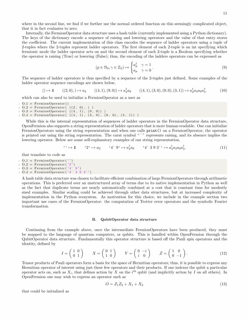
where in the second line, we find if we further use the normal ordered function on this seemingly complicated object,that it in fact evaluates to zero.

Internally, the FermionOperator data structure uses a hash table (currently implemented using a Python dictionary).The keys of the dictionary encode a sequence of raising and lowering operators and the value of that entry storesthe coefficient. The current implementation of this class encodes the sequence of ladder operators using a tuple of2-tuples where the 2-tuples represent ladder operators. The first element of each 2-tuple is an int specifying whichfermionic mode the ladder operator acts on and the second element of each 2-tuple is a Boolean specifying whetherthe operator is raising (True) or lowering (False); thus, the encoding of the ladders operators can be expressed as

(p ∈ N0, γ ∈ Z2) 7→

a†p γ = 1

ap γ = 0. (9)

The sequence of ladder operators is thus specified by a sequence of the 2-tuples just defined. Some examples of theladder operator sequence encodings are shown below,

() 7→ 11 ((2, 0), ) 7→ a2 ((4, 1), (9, 0)) 7→ a†4a9 ((4, 1), (3, 0), (9, 0), (3, 1)) 7→ a†4a3a9a†3. (10)

which can also be used to initialize a FermionOperator as a user as

1 O 1 = FermionOperator ( )2 O 2 = FermionOperator ( ( ( 2 , 0) , ) )3 O 3 = FermionOperator ( ( ( 4 , 1) , (9 , 0) ) )4 O 4 = FermionOperator ( ( ( 4 , 1) , (3 , 0) , (9 , 0) , (3 , 1) ) )

While this is the internal representation of sequences of ladder operators in the FermionOperator data structure,OpenFermion also supports a string representation of ladder operators that is more human-readable. One can initializeFermionOperators using the string representation and when one calls print() on a FermionOperator, the operatoris printed out using the string representation. The carat symbol “ ˆ ” represents raising, and its absence implies thelowering operator. Below are some self-explanatory examples of our string representation,

'' 7→ 11 '2' 7→ a2 '4ˆ 9' 7→ a†4a9 '4ˆ 3 9 3ˆ' 7→ a†4a3a9a†3. (11)

that translate to code as

1 O 1 = FermionOperator ( ' ' )2 O 2 = FermionOperator ( ' 2 ' )3 O 3 = FermionOperator ( ' 4ˆ 9 ' )4 O 4 = FermionOperator ( ' 4ˆ 3 9 3ˆ ' )

A hash table data structure was chosen to facilitate efficient combination of large FermionOperators through arithmeticoperations. This is preferred over an unstructured array of terms due to its native implementation in Python as wellas the fact that duplicate terms are nearly automatically combined at a cost that is constant time for modestlysized examples. Similar scaling could be achieved through other data structures, but at increased complexity ofimplementation in the Python ecosystem. As motivation for this choice, we include in the example section twoimportant use cases of the FermionOperator: the computation of Trotter error operators and the symbolic Fouriertransformation.

B. QubitOperator data structure

Continuing from the example above, once the intermediate FermionOperators have been produced, they mustbe mapped to the language of quantum computers, or qubits. This is handled within OpenFermion through theQubitOperator data structure. Fundamentally this operator structure is based off the Pauli spin operators and theidentity, defined by

I =

(1 00 1

)X =

(0 11 0

)Y =

(0 −ii 0

)Z =

(1 00 −1

). (12)

Tensor products of Pauli operators form a basis for the space of Hermitian operators; thus, it is possible to express anyHermitian operator of interest using just these few operators and their products. If one indexes the qubit a particularoperator acts on, such as Xi, that defines action by X on the ith qubit (and implicitly action by I on all others). InOpenFermion one may wish to express an operator such as

O = Z1Z2 +X1 +X2 (13)

that could be initialized as

12

1 from openfermion . ops import QubitOperator2 O = QubitOperator ( 'Z1 Z2 ' ) + QubitOperator ( 'X1 ' ) + QubitOperator ( 'X2 ' )

Similar to FermionOperator, QubitOperator is implemented internally using a hash table data structure throughthe native Python dictionary. This choice allows a good level of base efficiency for most arithmetic operators whileharnessing the features of the Python dictionary to ease implementation details. The keys used in this implementationare similarly tuples of tuples that define the type of operator and the qubit it acts on,

(O ∈ X,Y, Z, i ∈ N0) 7→ Oi. (14)

This internal representation may be used to initialize QubitOperators such as the operator X1X2 as

1 O = QubitOperator ( ( ( 1 , 'X ' ) , (2 , 'X ' ) ) )

or alternatively as seen above, a convenient string initializer is also available, which for the same operator could beused as

1 O = QubitOperator ( 'X1 X2 ' )

C. BosonOperator and QuadOperator data structures

In addition to the FermionOperator, OpenFermion also provides preliminary support for bosonic systems throughthe BosonOperator data structure. Like with fermionic systems, bosonic systems are commonly treated in secondquantization, using the symmetric bosonic creation and annihilation operators b†q and bq. These enforce bosonicstatistics by satisfying the canonical bosonic commutation relations,

[a†p, a†q] = [ap, aq] = 0, [a†p, aq] = δpq, (15)

and, analogously to the fermionic case, act on the vacuum state to create/annihilate bosons in the Fock space:

a†pn |vac〉 = |0, 0, . . . , 0︸ ︷︷ ︸

p−1

, n, 0, . . . , 0〉 . (16)

Due to these similarities, the BosonOperator is inherited from the same SymbolicOperator class as the FermionOp-erator, and thus retains many of the same properties, including the internal representation through the use of a hashtable, and forms of input (terms can be specified as a 2-tuple or in the more human-readable string representation).

For example, constructing the operator b†3b5b†1b4 can be done by the user as

1 from openfermion . ops import BosonOperator2 O = BosonOperator ( ’ 3ˆ 5 1ˆ 4 ’ )

Note that, unlike fermionic ladder operators, bosonic ladder operators acting on different subsystems commute pasteach other. Therefore, the terms of this operator will be stored as “1ˆ 3ˆ 4 5”, with indices ordered in ascending orderfrom left to right. To recover the unique “normal-ordered” form, with raising operators always to the left of loweringoperators, the user can use the normal ordered function provided to automatically rearrange the operator terms asper the commutation relations:

1 from openfermion . u t i l s import normal ordered2 normal ordered ( BosonOperator ( ’ 0 0ˆ ’ ) )

which returns “1.0 [ ] + 1.0 [0ˆ 0]”, corresponding to b0b†0 = I + b†0b0.

In addition to bosonic raising and lowering operators, it is common when studying bosonic systems to also considerdynamics in the phase space (q, p). The Hermitian position and momentum operators qi and pi act upon this phasespace, and are defined in terms of the bosonic ladder operators,

qi =

√~2

(bi + b†i

), pi = −i

√~2

(bi − b†i

). (17)

These operators are Hermitian, and are referred to as the quadrature operators. They satisfy the commutation relation[qi, pj ] = i~δij , where ~ depends on convention, often taking the values ~ = 0.5, 1, or 2.

In OpenFermion, the quadrature operators are represented by the QuadOperator class, and stored as a dictionaryof tuples (as keys) and coefficients (as values), similar to the QubitOperator. For example, the multi-mode quadratureoperator q0p1q3 is represented internally as ((0, ‘q’), (1, ‘p’), (3, ‘q’)). Alternatively, QuadOperators alsosupport string input — to initialize the latter operator using string representation, the user would enter the following:

13

1 from openfermion . ops import QuadOperator2 O = QuadOperator ( ’ q0 p1 q3 ’ )

As with the BosonOperator, quadrature operators acting on different subsystems commute, so the internal repre-sentation orders the terms with lowest index to the left. We also define a “normal-ordering” for quadrature operators,to allow a unique representation. The normal-ordered function introduced earlier rearranges the terms via the com-mutation relation such that position operators qi always appear to the left of momentum operators pi:

1 normal ordered (QuadOperator ( ’ p0 q0 ’ ) , hbar=2.)

Note that we now also pass the value ~ that appears in the commutation relation; if not provided, the default is ~ = 1.

Finally, OpenFermion provides functions for converting between the BosonOperator and QuadOperator:

1 from openfermion . t rans forms import get quad operator , g e t bo son ope ra to r2 O = QuadOperator ( ’ q0 p1 q3 ’ )3 O2 = get bo son ope ra to r (O, hbar=2.)

As before, we pass the value of ~ required depending on the convention chosen.

In addition to the functions and methods shown here, the BoseOperator and QuadOperator support additionaloperations (for example, sparse operator representations, symmetric ordering, and Weyl quantization of observablesin the phase space). They also form the basis for models provided by OpenFermion, such as the Bose-HubbardHamiltonian.

D. The MolecularData data structure

While the FermionOperator, BosonOperator, and QubitOperator classes form the backbone of many of the internalcomputations for OpenFermion, the data that defines a particular physical problem is more conveniently stored withina separate well-defined object, namely, the MolecularData object. This defines the schema by which the intermediatequantities calculated for the electronic structure of a molecule are stored, such as the two-electron integrals, basistransformation from the original basis, energies from correlated methods, and meta data related to the computation.For an exhaustive list of the current information stored within this class, it is recommended to see the documentation,as quantities are added as needed.

Importantly, this information is stored to disk in an HDF5 format using the h5py package. This allows for seamlessdata access to the files for only the quantities of interest, without the need for loading the whole file or complicatedinterface structures. Internally this is performed through the use of getters and setters using Python decorators, butthis is transparent to the user, needing only to get or set in the normal way, e.g.

1 two body in t eg ra l s = h2 molecu le . two body in t eg ra l s

where the data is read from disk on the access to two body integrals rather than when the object is instantiated inthe first line. This controls the memory impact of larger objects such as the two-electron integrals. Compressionfunctionality is also enabled through gzip to minimize the disk space requirements to store larger molecules.

Functionality is also built into MolecularData class to perform simple activate space approximations to the problem.An active space approximation isolates a subset of the total orbitals and treats the problem within that orbital set.This is done by modifying the one- and two-electron integrals as well as the count of active electrons and orbitals withinthe molecule. We assume a single reference for the active space definition and the occupied orbitals are integratedout according to the integrals while inactive virtual orbitals are removed. In OpenFermion this is as simple as takinga calculated molecule data structure, forming a list of the occupied spatial orbital indices (those which will be frozenin place) and active spatial orbital indices (those which may be freely occupied or unoccupied), and calling for somemolecule larger than H2 in a minimal basis

1 from openfermion . ops import In t e rac t i onOpera to r2

3 core cons tant , one body in t eg ra l s , two body in t eg ra l s = (4 molecule . g e t a c t i v e s p a c e i n t e g r a l s ( o c cup i ed ind i c e s , a c t i v e i n d i c e s ) )5 ac t i v e spa c e ham i l t on i an = Inte rac t i onOpera to r ( co re cons tant ,6 one body in t eg ra l s ,7 two body in t eg ra l s )

where active_space_hamiltonian can now be used to build quantum circuits for the reduced size problem.

14

E. The InteractionOperator data structure

As OpenFermion deals primarily with the interactions of physical fermions, especially electrons, the Hamiltonianwe have already introduced above

H = h0 +∑pq

hpqa†paq +

1

2

∑pqrs

hpqrsa†pa†qaras (18)

is ubiquitous throughout OpenFermion.Note that even for fewer than N = 100 qubits, the coefficients of the terms in the Hamiltonian of Eq. (18) can

require a large amount of memory. Since common Gaussian basis functions lead to the full O(N4) term scaling,instances with less than a hundred qubits can already have tens of millions to hundreds of millions of terms requiringon the order of ten gigabytes to store. Such large Hamiltonians can be expensive to generate (requiring nearly asmany integrals as there are terms) so one would often like to be able to save these Hamiltonians. While good forgeneral purpose symbolic manipulation, the FermionOperator data structure is not the most efficient way to storethese Hamiltonians, or to manipulate them with efficient numerical linear algebra routines, due to the extra overheadof storing each of the associated operators.

Towards this end we introduce the InteractionOperator data structure. This structure has already been seen inpassing in this document in the first example given. For example, with a MolecularData object, one may extract theHamiltonian in the form of an InteractionOperator through

1 h2 hami l ton ian = h2 molecu le . g e t mo l e cu l a r hami l t on i an ( )

where the Hamiltonian will be returned as an InteractionOperator. The InteractionOperator data structure is a classthat stores two different matrices and a constant. In the notation of Eq. (18), the InteractionOperator stores theconstant h0, an N by N array representing hpq and an N by N by N by N array representing hpqrs. Note thatat present this is not a spatially optimal representation if the goal is specifically to store the integrals of molecularelectronic structure systems, but it is a good compromise between space efficiency, simplicity, and ease of performingother numerical operations. The reason it is suboptimal is that there may exist symmetries within the integrals thatare not currently utilized. For example, there is an eight-fold symmetry in the integrals for real basis functions,hpqrs = hsqrp = hprqs = hsrqp = hqpsr = hrpsq = hqspr = hrspq. Note that for complex basis functions there isonly a four-fold symmetry. While we provide methods to iterate over these unique elements, we do not exploit thissymmetry in our current implementation for the reason that space efficiency of the InteractionOperator has not yetbeen a bottleneck in applications. This is consistent with our general design philosophy which is to maintain an activecycle of develop, test, profile, and refine. That is, rather than guess bottlenecks, we analyze and identify the mostimportant ones for problems of interest, and focus time there.

F. The InteractionRDM data structure

As discussed in the previous section, since fermions are identical particles which interact pairwise, their energy canbe determined entirely by reduced density matrices which are polynomial in size. In particular, these energies dependon the one-particle reduced density matrix (1-RDM), denoted here by (1)D and the two-particle reduced densitymatrix (2-RDM), denoted here by (2)D. The 1-RDM and 2-RDM of a fermionic wavefunction |ψ〉 are defined throughexpectation values with one- and two-body local FermionOperators;

(1)Dpq = 〈ψ| a†paq |ψ〉 (2)Dpqrs = 〈ψ| a†pa†qaras |ψ〉 . (19)

Thus, the 1-RDM is an N by N matrix and the 2-RDM is an N by N by N by N tensor. Note that the 1-RDMand 2-RDMs may (in general) represent a partial tomography of mixed states, in which case Eq. (19) should involvetraces over that mixed state instead of expectation values with a pure state. If one has performed a computation atthe CISD level of theory, it is possible to extract that density matrix from a molecule using the following command

1 c isd two rdm = h2 molecu le . get molecu lar rdm ( )

We can see that the energy of |ψ〉 with a Hamiltonian expressed in the form of Eq. (18) is given exactly as

〈E〉 = h0 +∑p,q

(1)Dpqhpq +1

2

∑p,q,r,s

(2)Dpqrshpqrs (20)

where h0, hpq and hpqrs are the integrals stored by the InteractionOperator data structure.

15

In OpenFermion, the InteractionRDM class provides an efficient numerical representation of these reduced densitymatrices. Both InteractionRDM and InteractionOperator inherit from a similar parent class, the PolynomialTensor,reflecting the close parallels between the implementation of these data structures. Due to this parallel, the exactsame code which implements integral basis transformations on InteractionOperator also implements integral basistransformations on the InteractionRDM data structure. Despite their similarities, they represent conceptually distinctconcepts, and in many cases should be treated in a fundamentally different way. For this reason the implementationsare kept distinct.

G. The QuadraticHamiltonian data structure

The general electronic structure Hamiltonian Eq. (18) contains terms that act on up to 4 sites, or is quartic inthe fermionic creation and annihilation operators. However, in many situations we may fruitfully approximate theseHamiltonians by replacing these quartic terms with terms that act on at most 2 fermionic sites, or quadratic terms,as in mean-field approximation theory. These Hamiltonians have a number of special properties one can exploitfor efficient simulation and manipulation of the Hamiltonian, thus warranting a special data structure. We refer toHamiltonians which only contain terms that are quadratic in the fermionic creation and annihilation operators asquadratic Hamiltonians, and include the general case of non-particle conserving terms as in a general Bogoliubovtransformation. Eigenstates of quadratic Hamiltonians can be prepared efficiently on both a quantum and classicalcomputer, making them amenable to initial guesses for many more challenging problems.

A general quadratic Hamiltonian takes the form∑p,q

(Mpq − µδpq)a†paq +1

2

∑p,q

(∆pqa†pa†q + ∆∗pqaqap) + constant, (21)

where M is a Hermitian matrix, ∆ is an antisymmetric matrix, δpq is the Kronecker delta symbol, and µ is achemical potential term which we keep separate from M so that we can use it to adjust the expectation of the totalnumber of particles. In OpenFermion, quadratic Hamiltonians are conveniently represented and manipulated usingthe QuadraticHamiltonian class, which stores M , ∆, µ and the constant from Eq. (21). It is specialized to exploitthe properties unique to quadratic Hamiltonians. Examples showing the use of this class for simulation are providedlater in this document.

H. Some examples justifying data structure design choices

Here we describe and show a few example illustrating that the above data structures are well designed for effi-cient calculations that one might do with OpenFermion. These examples are motivated by real use case examplesencountered in the authors’ own research. We do not provide code examples in all cases here but routines for thesecalculations exist within OpenFermion.

1. FermionOperator example: computation of Trotter error operators

Suppose that one has a Hamiltonian H =∑L`=1H` where the H` are single-term FermionOperators. Suppose now

that one decides to effect evolution under this Hamiltonian using the second-order Trotter formula, as investigated inworks such as [19, 25, 34–36]. A single second-order Trotter step of this Hamiltonian effects evolution under H + Vwhere V is the Trotter error operator which arises due to the fact that the H` do not all commute. In [35] it is shownthat a perturbative approximation to the operator V can be expressed as

V (1) = − 1

12

∑α≤β

∑β

∑γ<β

[Hα

(1− δα,β

2

), [Hβ , Hγ ]

]. (22)

Because triangle inequality upper-bounds to this operator provide an estimate of the Trotter error which can becomputed in polynomial time, symbolic computation of this operator is crucial for predicting how many Trotter stepsone should take in a quantum simulation. However, when using conventional Gaussian basis functions, Hamiltoniansof fermionic systems contain O(N4) terms, suggesting that the number of terms in Eq. (22) could be as high asO(N10). But in practice, numerics have shown that there is very significant cancellation in these commutators whichleads to a number of nontrivial terms that is closer to O(N4) after normal ordering [36]. If one were to use an array or

16

linked list structure to store FermionOperators then one has two choices. Option (i) is that new terms from the sumare appended to the list and then combined after the sum is completed. Under this strategy the space complexityof the algorithm would scale as O(N10) and one would likely run out of memory for medium sized systems. Option(ii) is that one normal orders the commutators before adding to the list and then loops through the array or listbefore adding each term. While this approach has average space complexity of O(N4), the time complexity of thisapproach would then be O(N14) as one would need to loop through O(N4) entries in the list after computing each ofthe O(N10) terms in the sum. Using our hash table implementation, the average space complexity is still O(N4) butone does not need to loop through all entries at each iteration so the time complexity becomes O(N10).

Though still quite expensive, one can use Monte Carlo based sampling or distribute this task on a cluster (it isembarrassingly parallel) to compute the Trotter error for medium sized systems. Using the Hamiltonian representa-tions introduced in [25], Hamiltonians have only O(N2) terms, which brings the number of terms in the sum down toO(N4) in the worst case. In that case, computation of V (1) would have time complexity O(N4) using the hash tableimplementation instead of O(N6) complexity using either a linked-list or an array. The O(N4) complexity enablesus to compute V (1) for hundreds of qubits, well into the regime of instances that would be classically intractable tosimulate. The task is even more efficient for Hubbard models which have O(N) terms.

2. FermionOperator example: symbolic Fourier transformation

A secondary goal for OpenFermion is that the library can be used to as a tool for the symbolic manipulation offermionic Hamiltonians in order to analyze and develop new simulation algorithms and Hamiltonian representations.To give a concrete example of this, in the recent paper [25], authors were able to demonstrate Trotter steps of theelectronic structure Hamiltonian with significantly reduced complexity: O(N) depth as opposed to O(N4) depth. Acritical component of that improvement was to represent the Hamiltonian using basis functions which are a discreteFourier transform of the plane wave basis (the plane wave dual basis) [25]. The appendices of that paper begin byshowing the Hamiltonian in the plane wave basis:

H =1

2

∑p,σ

k2p c†p,σcp,σ −

4π

Ω

∑p 6=qj,σ

(ζjei kp−q·Rj

k2q−p

)c†p,σcq,σ +

2π

Ω

∑(p,σ)6=(q,σ′)

ν 6=0

c†p,σc†q,σ′cq+ν,σ′cp−ν,σ

k2ν. (23)

To obtain the Hamiltonian in the plane wave dual basis, one applies the Fourier transform of the mode operators,

c†ν =

√1

N

∑p

a†pe−i kν ·rp cν =

√1

N

∑p

apei kν ·rp . (24)

Using OpenFermion one can easily generate the plane wave Hamiltonian (either manually or by using the plane wavemodule) and then apply the discrete Fourier transform of the mode operators (either manually or by using the discreteFourier transform module) to verify the correct form of the plane wave dual Hamiltonian shown in [25],

H =1

2N

∑ν,p,q,σ

k2ν cos [kν · rq−p] a†p,σaq,σ −4π

Ω

∑p,σj,ν 6=0

ζj ei kν ·(Rj−rp)

k2νnp,σ +

2π

Ω

∑(p,σ) 6=(q,σ′)

ν 6=0

cos [kν · rp−q]k2ν

np,σnq,σ′ . (25)

.While Eq. (25) turns out to have a very compact representation, it requires a careful derivation to show that

application of Eq. (24) to Eq. (23) leads to Eq. (25). However, this task is trivial for OpenFermion since the Fouriertransform can be applied symbolically and the output FermionOperator can be simplified automatically using anormal-ordering routine. This example demonstrates the utility of OpenFermion for verifying analytic calculations.

3. InteractionOperator example: fast orbital basis transformations

An example of an important numerical operation which is particularly efficient in this representation is a rotationof the molecular orbitals φp (r). This unitary basis transformation takes the form

φp (r) =

N∑q=1

φq (r)Upq U = e−κ κ = −κ† =∑p,q

κpqa†paq. (26)

17

For κ and U , the quantities κpq and Upq respectively correspond to the matrix elements of these N by N matrices.We see then that the O(N2) elements of the matrix κ define a unitary transformation on all orbitals. Often, onewould like to apply this transformation to Hamiltonian in the orbital basis defined by φp(r) in order to obtain a

new Hamiltonian in the orbital basis defined by φp(r). Since computation of the integrals is extremely expensive,the goal is usually to apply this transformation directly to the Hamiltonian operator.

When specialized to real, orthogonal rotations U (which is often the case in molecular electronic structure), themost straightforward expression of this integral transformation for the two-electron integrals is

hpqrs =∑

µ,ν,λ,σ

UpµUqνhµνλσUrλUsσ. (27)

Since there are O(N4) integrals, the entire transformation of the Hamiltonian would take time O(N8), which isextremely onerous. A more efficient approach is to rearrange this expression to obtain the following,

hpqrs =∑µ

Upµ

[∑ν

Uqν

[∑λ

Urλ

[∑σ

Usσhµνλσ

]]](28)

which can be evaluated for each term at cost O(N) since each summation can be carried out independently. Thisbrings the total cost of the integral transformation to O(N5). While such a transformation would be extremely tedioususing the FermionOperator representation, this approach is implemented for InteractionOperators in OpenFermionusing the einsum function for numerical linear algebra from numpy.

This functionality is readily accessible within OpenFermion for basis rotations. For example, the one may rotatethe basis of the molecular hamiltonian of H2 to a new basis with some orthogonal matrix U = exp(−κ) of appropriatedimension as

1 from numpy import array , eye , kron2

3 U = kron ( array ( [ [ 0 , 1 ] , [ 1 , 0 ] ] ) , eye (2 ) )4 h2 hami l ton ian = h2 molecu le . g e t mo l e cu l a r hami l t on i an ( )5 h2 hami l ton ian . r o t a t e b a s i s (U)

We now provide an example of where such fast basis transformations may be useful. Previous work has shown thatthe number of measurements required for a variational quantum algorithm to estimate the energy of a Hamiltoniansuch as Eq. (18) to precision ε scales as

M = O

[1

ε

∑p,q,r,s

|hpqrs|

]2 . (29)

Since the hpqrs are determined by the orbital basis, one can alter this bound by rotating the orbitals under anglesorganized into the κ matrix of Eq. (26). Thus, one may want to perform an optimization over these angles in orderto minimize M . This task would be quite unwieldy or perhaps nearly impossible using the FermionOperator datastructure but is viable using the InteractionOperator data structure with fast integral transformations.

4. QuadraticHamiltonian example: preparing fermionic Gaussian states

As mentioned above, eigenstates of quadratic Hamiltonians, Eq. (21), can be prepared efficiently on a quantumcomputer, and OpenFermion includes functionality for compiling quantum circuits to prepare these states. Eigenstatesof general quadratic Hamiltonians with both particle-conserving and non-particle conserving terms are also known asfermionic Gaussian states. A key step in the preparation of a fermionic Gaussian state is the computation of a basistransformation which puts the Hamiltonian of Eq. (21) into the form∑

p

εpb†pbp + constant, (30)

where the b†p and bp are a new set of fermionic creation and annihilation operators that also obey the canonicalfermionic anticommutation relations. In OpenFermion, this basis transformation is computed efficiently with matrixmanipulations by exploiting the special properties of quadratic Hamiltonians that allow one to work with only thematrices M and ∆ from Eq. (21) stored by the QuadraticHamiltonian class, using simple numerical linear algebra

18

routines included in SciPy. The following code constructs a mean-field Hamiltonian of the d -wave model of supercon-ductivity and then obtains a circuit that prepares its ground state (along with a description of the starting state towhich the circuit should be applied):

1 from openfermion . hami l ton ians import mean f ie ld dwave2 from openfermion . t rans forms import g e t quad ra t i c hami l t on i an3 from openfermion . u t i l s import g a u s s i a n s t a t e p r e p a r a t i o n c i r c u i t4

5 x dimension = 26 y dimension = 27 tunne l ing = 2 .8 sc gap = 2 .9 p e r i o d i c = True

10

11 mean f i e ld mode l = mean f ie ld dwave ( x dimension , y dimension , tunne l ing , sc gap , p e r i o d i c )12 quadra t i c hami l ton ian = ge t quadra t i c hami l t on i an ( mean f i e ld mode l )13 c i r c u i t d e s c r i p t i o n , s t a r t o r b i t a l s = g a u s s i a n s t a t e p r e p a r a t i o n c i r c u i t ( quadra t i c hami l ton ian )

The circuit description follows the procedure explained in [10]. One can also obtain the ground energy and groundstate numerically with the following code:

1 from openfermion . u t i l s import jw g e t g au s s i a n s t a t e2 ground energy , g round state = jw g e t g au s s i a n s t a t e ( quadra t i c hami l ton ian )

III. MODELS AND UTILITIES

OpenFermion has a number of capabilities that assist with the creation and manipulation of fermionic and relatedHamiltonians. While they are too numerous and growing too quickly to list in their entirety, here we will brieflydescribe a few of these examples in an attempt to ground what one would expect to find within OpenFermion.

One broad class of functions found within OpenFermion is the generation of fermionic and related Hamiltonians.While the MolecularData structure discussed above is one example for molecular systems, we also include utilities fora number of model systems of interest as well. For example, there are currently supported routines for generatingHamiltonians of the Hubbard model, the homogeneous electron gas (jellium), general plane wave discretizations, andd-wave models of superconductivity.

To give a concrete example, if one wished to study the homogeneous electron gas in 2D, which is of interest whenstudying the fractional quantum hall effect, then one could use OpenFermion to initialize the model as follows

1 from openfermion . hami l ton ians import j e l l i um mode l2 from openfermion . u t i l s import Grid3

4 j e l l i um hami l t on i an = je l l i um mode l ( Grid ( dimensions=2,5 l ength=10,6 s c a l e =1.0) )

where jellium hamiltonian will be a fermionic operator representing the spinful homogeneous electron gas discretizedinto a 10 × 10 grid of plane waves in two dimensions. One is then free to transform this Hamiltonian into qubitoperators and use it in the algorithm of choice.

Similarly, one may use the utilities provided to prepare a Fermi-Hubbard model for study. For example

1 from openfermion . hami l ton ians import fermi hubbard2

3 t = 1 .04 U = 4.05

6 hubbard hamiltonian = fermi hubbard ( x dimension=10, y dimension=10,7 tunne l ing=t , coulomb=U,8 ch em i c a l p o t en t i a l =0.0 , p e r i o d i c=True )

creates a Fermi-Hubbard Hamiltonian on a square lattice in 2D that is 10×10 sites with periodic boundary conditions.Besides Hamiltonian generation, OpenFermion also includes methods for outputting Trotter-Suzuki decompositions

of arbitrary operators, providing the corresponding quantum circuit in QASM format [87]. These methods wereincluded in order to simplify porting the resulting quantum circuits to other simulation packages, such as LIQUi| >[75], qTorch [79], Project-Q [70], and qHipster [88]. For instance, the function pauli exp to qasm takes a list ofQubitOperators and an optional evolution time as input, and outputs the QASM specification as a string. As anexample,

19

1 from openfermion . ops import QubitOperator2 from openfermion . u t i l s import pau l i exp to qasm3

4 f o r l i n e in pau l i exp to qasm ( [ QubitOperator ( 'X0 Z1 Y3 ' , 0 . 5 ) , QubitOperator ( 'Z3 Z4 ' , 0 . 6 ) ] ) :5 pr in t ( l i n e )

outputs a QASM specification for a circuit corresponding to U = e−i0.5X0Z1Y 3e−i0.6Z3Z4 , which in this case is givenby

1 H 02 Rx 1.5707963267948966 33 CNOT 0 14 CNOT 1 35 Rz 0 .5 36 CNOT 1 37 CNOT 0 18 H 09 Rx −1.5707963267948966 3

10 CNOT 3 411 Rz 0 .6 412 CNOT 3 4

OpenFermion additionally supports a number of other tools including the ability to evaluate the Trotter erroroperator and construct circuits for preparing arbitrary Slater determinants on a quantum computer using the lineardepth procedure described in [10]. Some support for numerical simulation is included for testing purposes, but theheavy lifting in this area is delegated to plugins specialized for these applications. In the future, we imagine theseutilities will expand to include more Hamiltonians and specializations that add in the creation of simulation circuitsfor fermionic systems.

IV. OPEN SOURCE MANAGEMENT AND PROJECT PHILOSOPHY

OpenFermion is designed to be a tool for both its developers and the community at large. By maintaining an open-source and framework independent library, we believe it provides a useful tool for developers in industry, academia,and research institutions alike. Moreover, it is our hope that these developers will, in turn, contribute code theyfound to be useful in interacting with OpenFermion to the benefit of the field as a whole. Here we outline some of ourphilosophy, as well as the ways in which we ensure that OpenFermion remains a high quality package, even as manydifferent developers from different institutions contribute.

A. Style and testing

The OpenFermion code is written primarily in Python with optional C++ backends being introduced as higherperformance is desired. Stylistically, this code follows the PEP8 guidelines for Python and demands descriptive namesas well as extensive documentation for all functions. This enhances readability and allows developers to more reliablybuild off of contributed code.

At present, the source code is managed through GitHub where the standard pull request system is used for makingcontributions. When a pull request is made, it must be reviewed by at least one member of the OpenFermion teamwho has experience with the library and is able to comment on both the style and integration prospects with thelibrary. As contributors become more familiar with the code, they may become approved reviewers themselves toenhance their contribution to the process. All contributors are welcome to assist with reviews but reviews from newcontributors will not automatically enable merging into the master branch.

Tests in the code are written in the python unittest framework and all code is required to be both Python 2 andPython 3 compliant so that it continues to be as useful as possible for all users in the future. The tests are runautomatically when a pull request is made through the Travis continuous integration (CI) framework, to minimize thechance that code that will break crucial functionality is accidentally merged into the code base, and ensure a smoothdevelopment and execution experience.

B. Distribution

Several options for code distribution are available to obtain OpenFermion. The code may be pulled and useddirectly from the GitHub repository if desired (which one can find at www.openfermion.org), and the requirements

20

may be manually fulfilled by the user. This option offers maximum control and access to bleeding edge code anddevelopments, but minimal convenience. A full service option is offered through the Python Package Index (PyPI) sothat installation for most users can be as simple as

1 python −m pip i n s t a l l openfermion

A middle ground between these options which is popular with many of the lead developers of this project is to pull thelatest code directly from GitHub but to install with pip using the development install command in the OpenFermiondirectory:

1 python −m pip i n s t a l l −e .

In the future, a version of the code may be supported for other distribution platforms as well.The OpenFermion plugins (and the packages on which they rely) need to be installed independently using a similar

procedure. One can install OpenFermion-Psi4 using pip under the name “openfermionpsi4”, OpenFermion-Cirq underthe name “openfermioncirq” and OpenFermion-PySCF under the name “openfermionpyscf”. These plugins can alsobe installed directly from GitHub (we link to repositories from the main OpenFermion page).

In addition to the traditional installation models of either installing from the PyPI registry, or downloading thesource from GitHub and installing, the project also supports a Docker container. Docker containers offer a compactvirtualization environment that is portable between all systems where Docker is supported. This is a convenient optionfor both first time users, and those who want to deploy OpenFermion to non-standard architectures (or on Windows).Moreover, it offers easy access to some of the electronic structure packages that our plugins are inter-operable with,which allows users convenient access to the full tool chain. At present, the Dockerfile is hosted on the repository,which can be used to build a Docker image as detailed in full in the Readme of the Docker folder.

CLOSING REMARKS

The rapid development of quantum hardware represents an impetus for the equally rapid development of quantumapplications. Development of these applications represents a unique challenge, often requiring the expertise or domainknowledge from both the application area and quantum algorithms. OpenFermion is a bridge between the world ofquantum computing and materials simulation, which we believe will act as a catalyst for development in this criticalarea. Only with such software tools can we start to explore the explicit costs and advantages of new algorithms,and push forward with practical advancements. It is our hope that OpenFermion not only leads to developments inthe field of quantum computation for quantum chemistry and materials, but also sparks the development of similarpackages for other application areas.

ACKNOWLEDGEMENTS

The authors thank Hartmut Neven for encouraging the initiation of this project at Google as well as Alan Aspuru-Guzik, Carlo Beenakker, Yaoyun Shi, Matthias Troyer, Stephanie Wehner and James Whitfield for supporting graduatestudent and postdoc developers who contributed code to OpenFermion. I. D. K. acknowledges partial support fromthe National Sciences and Engineering Research Council of Canada. K. J. S. acknowledges support from NSF GrantNo. 1717523. T. H. and D. S. S. have been supported by the Swiss National Science Foundation through the NationalCompetence Center in Research QSIT. S. S. is supported by the DOE Computational Science Graduate Fellowshipunder grant number DE-FG02-97ER25308. MS is supported by the Netherlands Organization for Scientific Research(NWO/OCW) and an ERC Synergy Grant.

[1] P. W. Shor, SIAM Journal on Computing 26, 1484 (1997).[2] A. W. Harrow, A. Hassidim, and S. Lloyd, Phys. Rev. Lett. 103, 150502 (2009).[3] R. P. Feynman, International Journal of Theoretical Physics 21, 467 (1982).[4] S. Lloyd, Science 273, 1073 (1996).[5] D. S. Abrams and S. Lloyd, Physical Review Letters 79, 4 (1997).[6] D. S. Abrams and S. Lloyd, Physical Review Letters 83, 5162 (1999).[7] G. Ortiz, J. Gubernatis, E. Knill, and R. Laflamme, Physical Review A 64, 22319 (2001).[8] R. D. Somma, G. Ortiz, J. E. Gubernatis, E. Knill, and R. Laflamme, Physical Review A 65, 17 (2002).[9] A. Aspuru-Guzik, A. D. Dutoi, P. J. Love, and M. Head-Gordon, Science 309, 1704 (2005).

21

[10] Z. Jiang, K. J. Sung, K. Kechedzhi, V. N. Smelyanskiy, and S. Boixo, Physical Review Applied 9, 044036 (2018).[11] D. Wecker, M. B. Hastings, N. Wiebe, B. K. Clark, C. Nayak, and M. Troyer, Physical Review A 92, 62318 (2015).[12] I. Kivlichan, N. Wiebe, C. Gidney, J. McClean, W. Sun, V. Denchev, A. Fowler, A. Aspuru-Guzik, and R. Babbush,

Unpublished (2018).

[13] L. Garcıa-Alvarez, I. L. Egusquiza, L. Lamata, A. del Campo, J. Sonner, and E. Solano, Physical Review Letters 119,040501 (2017).

[14] R. Babbush, D. Berry, and H. Neven, arXiv:1806.02793 (2018).[15] I. Kassal, S. P. Jordan, P. J. Love, M. Mohseni, and A. Aspuru-Guzik, Proceedings of the National Academy of Sciences

105, 18681 (2008).[16] N. J. Ward, I. Kassal, and A. Aspuru-Guzik, Journal Of Chemical Physics 130, 194105 (2008).[17] J. D. Whitfield, J. Biamonte, and A. Aspuru-Guzik, Molecular Physics 109, 735 (2011).[18] B. Toloui and P. J. Love, arXiv:1312.2579 (2013).[19] M. B. Hastings, D. Wecker, B. Bauer, and M. Troyer, Quantum Information & Computation 15, 1 (2015).[20] R. Babbush, D. W. Berry, Y. R. Sanders, I. D. Kivlichan, A. Scherer, A. Y. Wei, P. J. Love, and A. Aspuru-Guzik,

Quantum Science and Technology 3, 015006 (2018).[21] R. Babbush, D. W. Berry, I. D. Kivlichan, A. Y. Wei, P. J. Love, and A. Aspuru-Guzik, New Journal of Physics 18, 33032

(2016).[22] R. Babbush, P. J. Love, and A. Aspuru-Guzik, Scientific Reports 4 (2014), 10.1038/srep06603.[23] I. D. Kivlichan, N. Wiebe, R. Babbush, and A. Aspuru-Guzik, Journal of Physics A: Mathematical and Theoretical 50,

305301 (2017).[24] K. Sugisaki, S. Yamamoto, S. Nakazawa, K. Toyota, K. Sato, D. Shiomi, and T. Takui, The Journal of Physical Chemistry

A 120, 6459 (2016).[25] R. Babbush, N. Wiebe, J. McClean, J. McClain, H. Neven, and G. K.-L. Chan, Physical Review X 8, 011044 (2018).[26] F. Motzoi, M. P. Kaicher, and F. K. Wilhelm, Physical Review Letters 119, 160503 (2017).[27] I. D. Kivlichan, J. McClean, N. Wiebe, C. Gidney, A. Aspuru-Guzik, G. K.-L. Chan, and R. Babbush, Physical Review

Letters 120, 110501 (2018).[28] D. W. Berry, M. Kieferova, A. Scherer, Y. R. Sanders, G. H. Low, N. Wiebe, C. Gidney, and R. Babbush, npj Quantum

Information 4, 22 (2018).[29] R. Babbush, D. W. Berry, J. R. McClean, and H. Neven, arXiv:1807.09802 (2018).[30] D. Berry, C. Gidney, M. Motta, J. McClean, and R. Babbush, arXiv:1902.02134 (2019).[31] L. Veis and J. Pittner, Journal of Chemical Physics 133, 194106 (2010).[32] L. Veis and J. Pittner, Journal of Chemical Physics 140, 1 (2014).[33] J. R. McClean, R. Babbush, P. J. Love, and A. Aspuru-Guzik, The Journal of Physical Chemistry Letters 5, 4368 (2014).[34] D. Wecker, B. Bauer, B. K. Clark, M. B. Hastings, and M. Troyer, Physical Review A 90, 1 (2014).[35] D. Poulin, M. B. Hastings, D. Wecker, N. Wiebe, A. C. Doherty, and M. Troyer, Quantum Information & Computation

15, 361 (2015).[36] R. Babbush, J. McClean, D. Wecker, A. Aspuru-Guzik, and N. Wiebe, Physical Review A 91, 22311 (2015).[37] N. Rubin, R. Babbush, and J. McClean, New Journal of Physics 20, 053020 (2018).[38] J. T. Seeley, M. J. Richard, and P. J. Love, Journal of Chemical Physics 137, 224109 (2012).[39] J. D. Whitfield, Journal of Chemical Physics 139, 21105 (2013).[40] A. Tranter, S. Sofia, J. Seeley, M. Kaicher, J. McClean, R. Babbush, P. V. Coveney, F. Mintert, F. Wilhelm, and P. J.

Love, International Journal of Quantum Chemistry 115, 1431 (2015).[41] N. Moll, A. Fuhrer, P. Staar, and I. Tavernelli, Journal of Physics A: Mathematical and Theoretical 49, 295301 (2016).[42] J. D. Whitfield, V. Havlıcek, and M. Troyer, Physical Review A 94, 030301(R) (2016).[43] P. K. Barkoutsos, N. Moll, P. W. J. Staar, P. Mueller, A. Fuhrer, S. Filipp, M. Troyer, and I. Tavernelli, arXiv:1706.03637

(2017).[44] V. Havlıcek, M. Troyer, and J. D. Whitfield, Physical Review A 95, 32332 (2017).[45] S. Bravyi, J. M. Gambetta, A. Mezzacapo, and K. Temme, arXiv:1701.08213 (2017).[46] G. Zhu, Y. Subasi, J. D. Whitfield, and M. Hafezi, arXiv:1707.04760 (2017).[47] K. Setia and J. D. Whitfield, The Journal of Chemical Physics 148, 164104 (2018).[48] M. Steudtner and S. Wehner, New Journal of Physics 20, 063010 (2018).[49] M. Motta, E. Ye, J. R. McClean, Z. Li, A. J. Minnich, R. Babbush, and G. K.-L. Chan, arXiv:1808.02625 (2018).[50] Z. Jiang, J. McClean, R. Babbush, and H. Neven, arXiv:1812.08190 (2018).[51] N. Cody Jones, J. D. Whitfield, P. L. McMahon, M.-H. Yung, R. V. Meter, A. Aspuru-Guzik, and Y. Yamamoto, New

Journal of Physics 14, 115023 (2012).[52] M. Reiher, N. Wiebe, K. M. Svore, D. Wecker, and M. Troyer, Proceedings of the National Academy of Sciences 114,

7555 (2017).[53] R. Babbush, C. Gidney, D. Berry, N. Wiebe, J. McClean, A. Paler, A. Fowler, and H. Neven, Physical Review X 8, 041015

(2018).[54] B. P. Lanyon, J. D. Whitfield, G. G. Gillett, M. E. Goggin, M. P. Almeida, I. Kassal, J. D. Biamonte, M. Mohseni, B. J.

Powell, M. Barbieri, A. Aspuru-Guzik, and a. G. White, Nature Chemistry 2, 106 (2010).[55] Z. Li, M.-H. Yung, H. Chen, D. Lu, J. D. Whitfield, X. Peng, A. Aspuru-Guzik, and J. Du, Scientific Reports 1, 1 (2011).

22

[56] Y. Wang, F. Dolde, J. Biamonte, R. Babbush, V. Bergholm, S. Yang, I. Jakobi, P. Neumann, A. Aspuru-Guzik, J. D.Whitfield, and J. Wrachtrup, ACS Nano 9, 7769 (2015).

[57] R. Santagati, J. Wang, A. Gentile, S. Paesani, N. Wiebe, J. McClean, S. Short, P. Shadbolt, D. Bonneau, J. Silverstone,D. Tew, X. Zhou, J. OBrien, and M. Thompson, arXiv:1611.03511 (2016).

[58] A. Peruzzo, J. McClean, P. Shadbolt, M.-H. Yung, X.-Q. Zhou, P. J. Love, A. Aspuru-Guzik, and J. L. O’Brien, NatureCommunications 5, 1 (2014).

[59] M.-H. Yung, J. Casanova, A. Mezzacapo, J. McClean, L. Lamata, A. Aspuru-Guzik, and E. Solano, Scientific Reports 4,9 (2014).

[60] J. R. McClean, J. Romero, R. Babbush, and A. Aspuru-Guzik, New Journal of Physics 18, 23023 (2016).[61] Y. Shen, X. Zhang, S. Zhang, J.-N. Zhang, M.-H. Yung, and K. Kim, Physical Review A 95, 020501(R) (2017).[62] D. Wecker, M. B. Hastings, and M. Troyer, Physical Review A 92, 42303 (2015).[63] N. P. D. Sawaya, M. Smelyanskiy, J. R. McClean, and A. Aspuru-Guzik, Journal of Chemical Theory and Computation

12, 3097 (2016).[64] J. R. McClean, M. E. Kimchi-Schwartz, J. Carter, and W. A. de Jong, Phys. Rev. A 95, 042308 (2017).[65] P. J. J. O’Malley, R. Babbush, I. D. Kivlichan, J. Romero, J. R. McClean, R. Barends, J. Kelly, P. Roushan, A. Tranter,

N. Ding, B. Campbell, Y. Chen, Z. Chen, B. Chiaro, A. Dunsworth, A. G. Fowler, E. Jeffrey, A. Megrant, J. Y. Mutus,C. Neill, C. Quintana, D. Sank, A. Vainsencher, J. Wenner, T. C. White, P. V. Coveney, P. J. Love, H. Neven, A. Aspuru-Guzik, and J. M. Martinis, Physical Review X 6, 31007 (2016).

[66] J. I. Colless, V. V. Ramasesh, D. Dahlen, M. S. Blok, J. R. McClean, J. Carter, W. A. de Jong, and I. Siddiqi,arXiv:1707.06408 (2017).

[67] A. Kandala, A. Mezzacapo, K. Temme, M. Takita, J. M. Chow, and J. M. Gambetta, Nature 549, 242 (2017).[68] J. Romero, R. Babbush, J. McClean, C. Hempel, P. Love, and A. Aspuru-Guzik, Quantum Science and Technology 4,

14008 (2017).[69] C. Hempel, C. Maier, J. Romero, J. McClean, T. Monz, H. Shen, P. Jurcevic, B. Lanyon, P. Love, R. Babbush, A. Aspuru-

Guzik, R. Blatt, and C. Roos, Physical Review X 8, 031022 (2018).[70] D. S. Steiger, T. Haner, and M. Troyer, arXiv:1612.08091 (2016).[71] A. W. Cross, L. S. Bishop, J. A. Smolin, and J. M. Gambetta, arXiv:1707.03429 (2017).[72] R. S. Smith, M. J. Curtis, and W. J. Zeng, “A practical quantum instruction set architecture,” (2016).[73] A. S. Green, P. L. Lumsdaine, N. J. Ross, P. Selinger, and B. Valiron, in Proceedings of the 34th ACM SIGPLAN

Conference on Programming Language Design and Implementation, PLDI ’13 (ACM, New York, NY, USA, 2013) pp.333–342.

[74] P. Selinger, in Functional and Logic Programming (Springer Berlin Heidelberg, 2004) pp. 1–6.[75] D. Wecker and K. M. Svore, arXiv:1402.4467 (2014).[76] B. Valiron, N. J. Ross, P. Selinger, D. S. Alexander, and J. M. Smith, Commun. ACM 58, 52 (2015).[77] J. Heckey, S. Patil, A. JavadiAbhari, A. Holmes, D. Kudrow, K. R. Brown, D. Franklin, F. T. Chong, and M. Martonosi,

in ACM SIGARCH Computer Architecture News, Vol. 43 (ACM, 2015) pp. 445–456.[78] A. JavadiAbhari, S. Patil, D. Kudrow, J. Heckey, A. Lvov, F. T. Chong, and M. Martonosi, in Proceedings of the 11th

ACM Conference on Computing Frontiers (ACM, 2014) p. 1.[79] E. S. Fried, N. P. Sawaya, Y. Cao, I. D. Kivlichan, J. Romero, and A. Aspuru-Guzik, arXiv:1709.03636 (2017).[80] N. Killoran, J. Izaac, N. Quesada, V. Bergholm, M. Amy, and C. Weedbrook, arXiv preprint arXiv:1804.03159 (2018).[81] T. Helgaker, P. Jorgensen, and J. Olsen, Molecular Electronic Structure Theory (Wiley, 2002).[82] K. L. Schuchardt, B. T. Didier, T. Elsethagen, L. Sun, V. Gurumoorthi, J. Chase, J. Li, and T. L. Windus, Journal of

Chemical Information and Modeling 47, 1045 (2007), pMID: 17428029, http://dx.doi.org/10.1021/ci600510j.[83] R. M. Parrish, L. A. Burns, D. G. A. Smith, A. C. Simmonett, A. E. DePrince, E. G. Hohenstein, U. Bozkaya, A. Y.

Sokolov, R. Di Remigio, R. M. Richard, J. F. Gonthier, A. M. James, H. R. McAlexander, A. Kumar, M. Saitow, X. Wang,B. P. Pritchard, P. Verma, H. F. Schaefer, K. Patkowski, R. A. King, E. F. Valeev, F. A. Evangelista, J. M. Turney,T. D. Crawford, and C. D. Sherrill, Journal of Chemical Theory and Computation 13, 3185 (2017), pMID: 28489372,http://dx.doi.org/10.1021/acs.jctc.7b00174.

[84] Q. Sun, T. C. Berkelbach, N. S. Blunt, G. H. Booth, S. Guo, Z. Li, J. Liu, J. McClain, S. Sharma, S. Wouters, et al.,e-print arXiv:1701.08223 (2017).

[85] P. Jordan and E. Wigner, Zeitschrift fur Physik 47, 631 (1928).[86] S. Bravyi and A. Kitaev, Annals of Physics 298, 210 (2002).[87] A. W. Cross, L. S. Bishop, J. A. Smolin, and J. M. Gambetta, arXiv:1707.03429 (2017).[88] M. Smelyanskiy, N. P. D. Sawaya, and A. Aspuru-Guzik, “qHiPSTER: The Quantum High Performance Software Testing

Environment,” (2016), arXiv:1601.07195.