Embed Size (px)
Citation preview

Ontology Construction for Information Selection1
Latifur Khan and Feng Luo Department of Computer Science
University of Texas at Dallas Richardson, TX 75083-0688
Email: [lkhan, luofeng]@utdallas.edu
Abstract
Technology in the field of digital media generates huge amounts of textual information. The potential for exchange and retrieval of information is vast and daunting. The key problem in achieving efficient and user-friendly retrieval is the development of a search mechanism to guarantee delivery of minimal irrelevant information (high precision) while insuring relevant information is not overlooked (high recall). The traditional solution employs keyword-based search. The only documents retrieved are those containing user specified keywords. But many documents convey desired semantic information without containing these keywords. One can overcome this problem by indexing documents according to meanings rather than words, although this will entail a way of converting words to meanings and the creation of ontologies. We have solved the problem of an index structure through the design and implementation of a concept-based model using domain-dependent ontologies. Ontology is a collection of concepts and their interrelationships, which provide an abstract view of an application domain. We propose a new mechanism that can generate ontologies automatically in order to make our approach scalable. For this we modify the existing self-organizing tree algorithm (SOTA) that constructs a hierarchy. Furthermore, in order to find an appropriate concept for each node in the hierarchy we propose an automatic concept selection algorithm from WordNet, a linguistic ontology. To illustrate the effectiveness of our automatic ontology construction method, we have explored our ontology construction in text documents. The Reuters21578 text document corpus has been used. We have observed that our modified SOTA outperforms hierarchical agglomerative clustering (HAC).
Keywords: Ontology, Clustering, Self Organizing Tree, WordNet.
1 This study was supported in part by gift from Sun and the National Science Foundation grant, NGS-0103709.

1. Introduction
The development of web technology generates huge amounts of textual information [21].
The potential for the exchange and retrieval of information is vast, and at times daunting.
In general, users can be easily overwhelmed by the amount of information available via
electronic means. The transfer of irrelevant information in the form of documents (e.g.
text, audio, video) retrieved by an information retrieval system and which are of no use to
the user wastes network bandwidth and creates user frustration. This condition is a result
of inaccuracies in the representation of the documents in the database, as well as
confusion and imprecision in user queries, since users are frequently unable to express
their needs efficiently and accurately. These factors contribute to the loss of information
and to the retrieval of irrelevant information. Therefore, the key problem to be addressed
in information selection is the development of a search mechanism which will guarantee
the delivery of a minimum of irrelevant information (high precision), as well as insuring
that relevant information is not overlooked (high recall).
The traditional solution to the problem of recall and precision in information retrieval
employs keyword-based search techniques. Documents are only retrieved if they contain
keywords specified by the user. However, many documents contain the desired semantic
information, even though they do not contain user specified keywords. This limitation
can be addressed through the use of query expansion mechanisms. Additional search
terms are added to the original query based on the statistical co-occurrence of terms [22].
Recall will be expanded, but at the expense of deteriorating precision [24, 25]. In order to
overcome the shortcomings of keyword-based technique in responding to information

selection requests we have designed and implemented a concept-based model using
ontologies [19, 26, 27]. This model, which employs a domain dependent ontology, is
presented in this paper. Ontology is a collection of concepts and their interrelationships
which can collectively provide an abstract view of an application domain [11, 12].
There are two distinct problem/tasks for an ontology-based model: one is the extraction
of semantic concepts from the keywords and the other is the actual construction of the
ontology. With regard to the first problem, the key issue is to identify appropriate
concepts that describe and identify documents. In this it is important to make sure those
irrelevant concepts will not be associated and matched, and that relevant concepts will
not be discarded. With regard to the second problem, we would like to construct
ontologies automatically. In this paper we address these two problems together by
proposing a new method for the automatic construction of ontology.
Our method constructs ontology automatically in top-down fashion. For this, we first
construct a hierarchy using some clustering algorithms. Recall that if documents are
similar to each other in content they will be associated with the same concept in ontology.
Next, we need to assign a concept for each node in the hierarchy. For this, we deploy two
types of strategy and adopt a bottom up concept assignment mechanism. First, for each
cluster consisting of a set of documents we assign a topic based on a supervised self-
organizing map algorithm for topic tracking. However, if multiple concepts are candidate
for a topic we propose an intelligent method for arbitration. Next, to assign a concept to
an interior node in the hierarchy we use WordNet, a linguist ontology [5, 6]. Descendant
concepts of the internal node in the hierarchy will also be identified from WordNet.

From these identified concepts and their hypernyms we can identify a more generic
concept that can be assigned as a concept for the interior node.
With regard to the hierarchy construction, we would like to construct ontology
automatically. For this we rely on a self-organizing tree algorithm (SOTA [4]) that
constructs a hierarchy from top to bottom. We modify the original algorithm, and propose
an efficient modified SOTA (MSOT) algorithm.
To illustrate the effectiveness of the method of automatic ontology construction, we have
explored our ontology construction in the text documents. The Reuters21578 text
document corpus has been used. We have observed that our modified SOTA out performs
hierarchical agglomerative clustering (HAC). The main contributions of this work will
be as follows:
• We propose a new mechanism that can be used to generate ontology
automatically to make our approach scalable. For this, we modify the existing
self-organizing tree algorithm (SOTA) that constructs a hierarchy from top to
bottom.
• Furthermore, to find an appropriate concept for each node in the hierarchy we
propose an automatic concept selection algorithm from WordNet, a linguistic
ontology.
Section 2 discusses related works. Section 3 describes ontologies and their
characteristics. Section 4 presents our automatic ontology construction mechanism.
Section 5 presents result. Section 6 contains our conclusion and possible areas of future
work.

2. Related Work
Historically ontology has been employed to achieve better precision and recall in the text
retrieval system [18, 20]. Here, attempts have taken two directions, query expansion
through the use of semantically related-terms, and the use of conceptual distance
measures [22, 25, 26, 27].
For the construction of ontology, the above papers assume manual construction; however,
only a few automatic methods are proposed [23, 28, 29]. Elliman et al. [28] propose a
method for constructing ontology to represent a set of web pages on a specified site. Self
organizing map is used to construct hierarchy. Bodner et al. [23] propose a method to
construct hierarchy based on statistical method (frequency of words). Hotho et al. [29]
propose various clustering techniques to view text documents with the help of ontology.
Note that a set of hierarchies will be constructed for multiple views only; not for ontology
construction purpose.
3. Ontology for Information Selection
Ontology is a specification of an abstract, simplified view of the world that we wish to
represent for some purpose [10, 11, 12]. Therefore, ontology defines a set of
representational terms that we call concepts. Inter-relationships among these concepts
describe a target world. Ontology can be constructed in two ways, domain dependent and
generic. CYC [13, 14], WordNet [5, 6], and Sensus [16] are examples of generic
ontology. WordNet is a linguistic database formed by synsets—terms grouped into
semantic equivalence sets, each one assigned to a lexical category (noun, verb, adverb,
adjective). Each synset represents a particular lexical concept of an English word and is

usually expressed as a unique combination of synonym sets. In general, each word is
associated to more than one synset and more than one lexical category.
Figure 1. A Portion of Ontology for Sports Domain
A domain-dependent ontology provides concepts in a fine grain, while generic ontology
provides concepts in coarser grain. Figure 1 illustrates example ontology for the sports
domain. This ontology may be obtained from generic sports terminology and domain
experts [17]. The ontology is described by a directed acyclic graph (DAG). Here, each
node in the DAG represents a concept. In general, each concept in the ontology contains
a label name and a vector. A vector is simply a set of keywords and their weights.
Furthermore, the weight of each keyword of a concept may not be equal. In other words,
for a particular concept some keyword may serve as more discriminating as compared to
some other; it will be assigned higher weight.
In Ontology, concepts are interconnected by means of inter-relationships. If there is a
inter-relationship R, between concepts Ci and Cj, then there is also a inter-relationship R′
between concepts Cj and Ci. In Figure 1, inter-relationships are represented by labeled
arcs/links. Three kinds of inter-relationships are used to create our ontology: IS-A,

Instance- Of, and Part-Of. These correspond to key abstraction primitives in object-based
and semantic data models.
4. Automated Ontology Construction
We would like to build ontology automatically from a set of text documents. If
documents are similar to each other in content they will be associated with the same
concept in ontology. For this first we would like to use a hierarchical clustering algorithm
to build a hierarchy. Then we need to assign concept for each node in the hierarchy. For
this, we deploy two types of strategy and follow bottom up concept assign mechanism.
First, for each cluster consisting of a set of documents we assign a topic based on a
supervised self-organizing map algorithm for topic tracking. However, if multiple
concepts are candidates for a topic we propose an intelligent method to arbitrate them.
Next, to assign concept to the interior node in the hierarchy, we use WordNet, a linguist
ontology. Descendant concepts of the internal node in the hierarchy will be identified in
WordNet. From these identified concepts and their hypernyms we can identify more
generic concept that can be assigned as a concept for the interior node.
First, we will present various hierarchical construction methods. Then we will present our
proposed methods for assigning concepts in the hierarchy, including topic tracking and
concept sense disambiguation.
4.1 Hierarchy Construction
We would like to partition a set of documents S= {D1, D2… Dn} into a number of clusters
C1, C2… Cm, where a cluster may contain more than one documents. Furthermore, we
would like to extend our hierarchy into several levels. For this, several existing

techniques are available to such as hierarchical agglomerative clustering (HAC) [1], self-
organizing map (SOM) [7], self-organizing tree (SOTA) [4], and so on.
4.1.1. Self-Organizing Map (SOM)
The SOM, introduced by Kohonen [7], is one of the unsupervised neural networks. A
SOM consists of two parts, the input data (i.e., document, image) and the output map. It
maps the high dimensional input data into the low dimensional output topology space,
which is two-dimensional. Furthermore, we can think of the SOM as a “nonlinear
projection” of probability density function p(x) of the high-dimensional input data vector
x onto the two dimensional display. This makes SOM optimally suitable for application
to the problem of the visualization and cluster of complex data.
Each SOM input data is represented by a vector of features x. Each node in the output
map has a reference vector w. The reference vector has the same dimension as the feature
vector of input data. Figure 2 shows the basic architecture of SOM. Initially the reference
vector is assigned to random values. During the learning process an input data vector is
randomly chosen from the input data set and compare with all w. Various distance
measure functions can be used to compare such as Euclidean distances ||x-wi|| or cosine
distances (x,wi)/(||x||*||wi||). The best matching node c is the node, which has the
minimum distance with the input data.
}||{||min||:|| iic wxwxc −=− (1)
Then the reference vector of the best matching node and its neighboring nodes which are
topologically close in the map are updated by Equation 2. In this way, eventually
neighboring nodes will become more similar to the best match nodes. Therefore, the
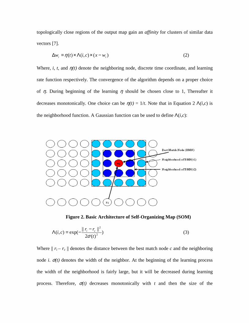
topologically close regions of the output map gain an affinity for clusters of similar data
vectors [7].
)(),()( ii wxcitw −×Λ×=∆ η (2)
Where, i, t, and η(t) denote the neighboring node, discrete time coordinate, and learning
rate function respectively. The convergence of the algorithm depends on a proper choice
of η. During beginning of the learning η should be chosen close to 1, Thereafter it
decreases monotonically. One choice can be η(t) = 1/t. Note that in Equation 2 Λ(i,c) is
the neighborhood function. A Gaussian function can be used to define Λ(i,c):
Figure 2. Basic Architecture of Self-Organizing Map (SOM)
))(2
||||exp(),( 2
2
trrci ci
σ−
−=Λ (3)
Where || ri – rc || denotes the distance between the best match node c and the neighboring
node i. σ(t) denotes the width of the neighbor. At the beginning of the learning process
the width of the neighborhood is fairly large, but it will be decreased during learning
process. Therefore, σ(t) decreases monotonically with t and then the size of the

neighborhood also monotonically decreases. At the end of learning only the best match
node is updated. The learning steps will stop when the weight update is insignificant.
4.1.2. Self-Organizing Tree Algorithm (SOTA)
The predetermined structure of classical SOM implies a limitation on the result mapping.
A number of models have been proposed to build a topology of output nodes. Fritzke [8]
proposes a growing cell structure (GCS) model which facilitates finding the suitable
output mapping structure and size automatically. Based on the SOM and GCS, Dopazo et
al. [4] introduce a new unsupervised growing and tree-structured SOM called self-
organizing tree algorithm (SOTA) [9]. The topology of SOTA is a binary tree.
Figure3. (A) Initial Architecture of SOTA
(B) Two Different Reference Vector Updating Schemes
Initially the system is a binary tree with three nodes (Figure 3 (A)). The leaf of the tree is
called cell and internal node of the tree is called node. Each cell and the node have a
reference vector w. The values of the reference vector are randomly initialized. In SOTA
only cells are used for comparing with the input data. After distributing all the input data
into two cells, the cell which is most heterogeneous will be changed itself to a node and
create two descendent cells. This procedure is called cycle. To determine heterogeneity a

Resource is introduced. Resource of a cell i is calculated based on the average of the
distances of the input data assigned to the cell from cell vector.
∑=
=D
j
iii D
wxdsource
1
),(Re (4)
Where D is the total number of input data associated with the cell. A cell which has the
maximum Resource will expand. Therefore, the algorithm proceeds the cycle until each
input data is associated with a single cell or it reach at the desired level of heterogeneity.
Each adaptation cycle is contained a series of epochs. Each epoch consists of presentation
of all the input data and each presentation has two steps. First, we find the best match cell
which is known as winning cell. This is similar to the SOM. The cell that has the
minimum distance with the input data is the best match cell/winning cell. The second is
updating the reference vector wi of winning cell and its neighborhood using the following
function:
)()( ii wxtw −×=∆ ϕ (5)
Where ϕ(t) is the learning function:
)()( tt ηαϕ ×= (6)
η(t) is function similar in SOM and α is a learning constant. For different neighbors α
have different values. Two different neighborhoods are here. If the sibling of the winning
cell is a cell, then the neighborhood includes the winning cell, the parent node and the
sibling cell. On the other hand, it includes only the winning cell itself [4] (see Figure 3
(B)). Furthermore, parameters αw, αm and αs are used for the winning cell, the ancestor
node and the sibling cell, respectively. For example, values of αw, αm and αs can be set as
0.1, 0.05, and 0.01 respectively. Note that parameter values are not equal. This is because

these non-equal values are critical to partition the input data set into various cells. A cycle
is converged when the relative increase of total error falls below a certain threshold.
4.1.3. Modified SOTA
SOTA is specifically designed for molecular bio-sequence classification and
phylogenetic analysis. Inspired by the self-organized tree structure and low time
complexity we develop a modified self-organizing tree for image classification which is
called MSOT.
Figure 4. Ontology Construction A) SOTA B) MSOT
Although MSOT is similar to SOTA, it differs in two ways. First, in SOTA, during
expansion, only one cell, which has the maximum resources, will be selected for
expansion. On the other hand, in MSOT more than one cell may be selected for
expansion, depending on their resources (see Figure 4). Here cells whose resources
exceed a threshold will participate in the expansion. Thus, the aspect of threshold plays
an important role here. Expansion of more than one node allows the algorithm to grow a
tree quickly. Second, in SOTA during the expansion phase of a selected node two new
cells will be created. Furthermore, initially each new cell will replicated with the same

reference vector of the selected cell. Now, input data associated with selected node will
be distributed between two new cells; the reference vector of each new cell will be
updated. Therefore, input data will only be considered for the distribution of within two
new cells, (i.e., locally). On the other hand, in MSOT more than one node may be
selected, and two new cells will be created for each selected node. Now the question is
how we can distribute input data of selected node among these new created cells. One
approach is that input data of each selected node will be distributed to two new created
children cells which are similar to the SOTA approach. This kind of distribution cannot
provide a good cluster result because data may be poorly distributed between two new
cells. Furthermore, once data is wrongly assigned in a group at earlier stage we cannot
adjust them later. This is also one of the shortcomings of the classical HAC algorithm.
The other approach is aggressive; input data of selected node will be distributed not only
its new created cells but also its neighbor cells. For this, first we determine K level apart
ancestor node of selected node. Next, we determine a sub-tree rooted by the ancestor
node and input data of selected cell will be distributed among all cells (leaf) of this sub-
tree. The latter approach is known as K level distribution (KLD).
Figure 5. Two Level Distribution Scope of MSOT

For example, Figure 5 shows the scope of K=1. Now, we need to distribute data
associated with node M to new created cells. For K=1, immediate ancestor of M will be
determined which is A. Data of node M will be distributed to cells (i.e., B, C, D, and E)
of a sub-tree rooted by A. For each data we will determine winning cell among B, C, D,
and E using Equation 1. Note that if K=0, data of M will be distributed between cells B
and C; the latter approach is simply turned into the former approach. After distributing
each input data, winning cell and neighbor reference vector will be updated.
The pseudo code for the MSOT algorithm is as follows:
Step 1: [Initialization] initialize as like as SOTA—one node with two cells.
Step 2: [Distribution] distribute each input data between newly created cells; find
the winning cell using KLD and assign the input data to this winning cell, update the
reference vector of the winning cell and its neighbor using Equation 5 & 6.
Step 3: [Error] while error of the entire tree is larger than a threshold go back to
Step 2.
Step 4: [Expand] for each cell, calculate resource, and check whether it exceeds a
threshold. If yes, change this selected cell as node, and create two new children cells
from it. If there are no more cells for expansion, the system is converged; else go back to
Step 2.
Step 5: prune the tree and delete a cell that does not have any input on it.
4.2 Concept Assignment
After building a hierarchy of nodes we will assign a concept for each node in the
hierarchy. For this, we propose a bottom up mechanism for assigning concepts. Concepts
associated with documents will be assigned to leaf nodes in the hierarchy. Interior node

concepts will then be assigned based on the concepts in the descendent nodes. For each
cluster consisting of a set of documents we will assign a topic based on a supervised self-
organizing map algorithm for topic tracking. Second, we will associate this topic with an
appropriate concept (synset) in WordNet. Third, the concept of an internal node is
obtained from concepts of its children nodes and their hypernyms as they in WordNet.
4.2.1 Concept Assignment for Leaf Nodes
Topic tracking is used for the assignment of a concept in each leaf node. For this, a topic
will first be assigned for each document. Second, we will determine the distinct topics
that appear in each leaf node. Recall that a leaf node may be associated with a number of
different documents. Now, if only a single topic appears in a leaf node, we will simply
assign this topic as a concept in the leaf node. However, if more than one topic appears in
a leaf node, a majority rule will be applied. Thus, a majority of documents of a leaf node
will be associated with a specific topic and this topic will be assigned as a concept to this
leaf node. This majority threshold depends on a degree of generalization and it is
determined experimentally; in our case we chose 70%. On the other hand, in cases in
which the majority rule cannot be applied, we will choose a more generic concept from
WordNet using all the topics, and this generic concept will be assigned (see Section
4.2.2).
4.2.1.1 Topic Tracking
Here we will determine a topic for each document. For this we assume we have a set of
predefined topic categories. The topic categories are trained by a set of documents
previously assigned to existing topics. Each topic is represented by a keyword. Here we

assume that only one topic is assigned per document. This is because a document can be
associated with at most one node in the hierarchy.
We will consider the classical Rocchio algorithm [2, 3] and supervised SOM algorithm
for topic tracking. The basic idea of Rocchio algorithm is to construct a document vector
to represent the document and a topic vector for each topic. Documents with the same
topic have the same topic vector. For a given topic the topic vector is the topic
representative vector of the documents assigned to this topic category. To determine a
topic for a document, the similarity between a document and a topic vector is measured
using the cosine product. We will choose the topic for the document which this
calculation of similarity gives the maximum value.
The document vector is built by weighting all the words in documents with the tf (d, w) *
idf(w) value. The term frequency tf is the number of times word w occurs in a document
d. The document frequency df(w) is the number of documents in which the word w
occurs at least once. The inverse documents frequency idf(w) is commonly defined as
follows:
))(
log()(wdf
Nwidf = (7)
N is the total number of documents. A word which appears in fewer documents will have
a higher IDF. The word with higher tf*idf weighting means it is an important index term
for the document.
In the classical Rocchio algorithm the topic vector t is built by combining the document
vectors d of the training documents.
∑⊂
=Tddt�
�
(8)

Where T is the topic and d is a document.
We will also use supervised SOM algorithm to construct topic vector. Each topic
category is represented by a node in the SOM’s output map. To construct the topic
vector, the node is trained by training documents that belong to that topic. The reference
vector of the node is the centroid vector of these trained document vectors, constructed
by a nonlinear regression. This reference vector will then be the topic vector.
Once topic vectors have been constructed we will use the cosine of document vector and
topic vector to score the similarity (see Equation 9).
∑∑
∑
==
=
×
×= n
kjk
n
kik
n
kjkik
dd
dddjdiSimilarity
1
2
1
2
1
)()(
)(),(
��
��
(9)
4.2.1.2 Concept Sense Disambiguation
It is possible that a particular keyword may be associated with more than one concept in
WordNet. In other words, association between keyword and concept is one:many, rather
than one:one. For example the keyword “gold” has 4 senses in WordNet and the
keyword “copper” has five senses in WordNet. We need to disambiguate keywords and
choose the most appropriate concept.
For disambiguation of concepts we apply the same technique (i.e., cosine similarity
measure) used in topic tracking. To construct a vector for each sense we will use a short
description that appears in WordNet.
4.2.2 Concept Selection for Non Leaf Nodes
To assign a concept to an internal node in the tree we need to consider similar cases. If
two children of a node have the some concept we merely assign that concept to the parent
node. If two children have a different concept but one concept belongs to the majority

(i.e. 70%) we will assign this majority concept to the parent node. And if there is no
majority concept we will find an appropriate concept for parent node using WordNet. We
will find all the parent senses of two children topic concepts. Then we will select the least
general concept sense and assign it to the parent node. For example, “gold” and “copper”
are associated with a set of documents and majority rule will not be applicable in this
case. We will select the least generic concept (i.e., “asset”) of these two senses, and
assign to their parent node.
5. Preliminary Result
5.1 Experimental Setup
We have explored our ontology construction using text documents. The Reuters21578
text document corpus was used. There are 135 topics assigned to the Reuters documents.
We selected 2003 documents from this corpus distributed across 15 topics. Furthermore,
each document has only one topic. 180 of these documents were used for topic tracking
training. Note that documents are not distributed across topics uniformly. In other words,
one given topic may have more documents as compared to another. Thus, the greater the
number of documents in a given topic, the greater the number of training documents
employed.
For document processing we have extracted keywords (terms) from documents by
removing stop words. Second, using the Porter stemming [31] technique we have
determined word stems. Third, we have constructed a document vector for each
document using tf*idf.

5.1.1 Experimental Evaluation
We use Recall, Precision and E measure [30] to evaluate our clustering algorithms and
topic tracking algorithms. Recall is the ratio of relevant documents to total documents for
a given topic. Precision is the ratio of relevant documents to documents which appear in
a cluster for a given topic. E measure is defined as follows:
rp
rpE11
21),(+
−= (10)
Where p and r are the Precision and Recall of a cluster. Note that E (p, r) is simply one
minus harmonic mean of the precision and recall; E (p, r) ranges from 0 to 1 where E (p,
r) =0 corresponds to perfect precision and recall, and E (p, r) corresponds to zero
precision and recall. Thus, the smaller the E measure value the better the result of an
algorithm.
5.2 Results
First, we will present the results for the topic tracking algorithm. Second, we will present
the clustering results of HAC and MSOT. Finally, we will report the performance of our
concept selection mechanism for each node in hierarchy.
5.2.1 Topic Tracking Algorithm Comparison
For the classical Rocchio algorithm, we first constructed a topic vector for each topic.
The weight of each term in a topic is simply the summation of weights of the term in the
training documents. Next, we have sorted terms based on weight in descending order.
Then we have used first l (=50,100, 200,400) keywords to reduce dimensionality.
In the supervised SOM we have constructed a reference vector for each topic. The weight
of the term was assigned randomly. Then reference vector of a topic was updated using

SOM whenever a document is associated with that topic. Furthermore we used first l
keywords to reduce dimensionality.
0.10.105
0.110.1150.12
0.1250.13
0.135
0.140.145
50 100 200 400
l
ESupervised SOMClassical Rocchio
Figure 6. Results of Topic Tracking
Figure 6 shows the result of the classical Racchio and the supervised SOM. X and Y axis
of Figure 6 represent l and average E measure respectively. These two algorithms get
almost the same result. However, only when l=100 the supervised SOM gets slightly
better result than the classical Racchio. The topic vector of supervised SOM uses the
centroid of all training document vector. It represents the topic better than the topic
vector in classical Racchio, which is the simple summation of all training document
vector. After l=200 the topic tracking result of these two algorithm was the same. So we
chose l=200 supervised SOM for the rest of experiments.
5.2.2. Optimizing of MSOT Parameters
In our experiment we varied αw (i.e., =0.1, 0.15, 0.2, 0.25, 0.3) and αs (i.e., =0.01, 0.015,
0.02, 0.025, 0.03). Furthermore, αm is set as 0.5 of αw, η(t) is set as 1/t, and KLD is set to
3 (see Section 4.1.2). Thus, we got total 25 combinations, and for each combination, we
calculated E.

In Figure 7 X and Y axis represent winner learning constant, αw and average E of MOST
respectively for a fixed αs. Figure 7 shows how the combination of sibling learning
constant, αs and αw affect the clustering result. When αw =0.2 and αs=0.02 we get the
lowest E (= 0.073) which is the best case in our test.
0.06
0.07
0.08
0.09
0.1
0.11
0.12
0.13
0.14
0.1 0.15 0.2 0.25 0.3
winner learning constant
E
sibling learning contant = 0.01sibling learning contant = 0.015sibling learning contant = 0.02sibling learning contant = 0.025sibling learning contant = 0.03
Figure 7. E Measure of MOST on Various Parameters
0.050.07
0.090.110.13
0.150.170.19
0.210.23
0 1 2 3
K Level Distribution
E
Figure 8. E Measure of MSOT for Different K-Level Distribution

5.2.3. The Result of K-Level Distribution
We test how different K-Level distribution affects the clustering result. The parameter of
the test is set as: αw=0.2 αm=0.1 and αs=0.02. These parameter settings gave better results
in Figure 7. In Figure 8 X and Y axis represent K Level and average E measure
respectively. Figure 8 shows when K increases from 0 to 1 the clustering result has been
improved greatly and E reduces from 0.213 to 0.087. This demonstrates that data has
been poorly distributed when K=0. The KLD overcome this by redistributing the data to
the more number of groups (cells). Figure 8 also shows after K>2 the cluster result does
not change. So, we chose K = 2 in the rest of experiments.
5.2.4. Hierarchy Construction Comparison
We have compared MSOT with group-average link HAC. We have used the original
topic of the Reuters news items to evaluate the result of these cluster algorithms. Since
αw=0.2 αm=0.1 and αs=0.02 give least error (E), we used these values. Note that
documents are only associated with leaf nodes. We have observed that the boundary of a
cluster is very clear and clean in MSOT. Furthermore, MSOT gives a better result than
HAC (see Figure 9). In all topics MSOT have low E measure than HAC. Finally, the
average E of MSOT is 0.073 while the average E of HAC is only 0.181.

00.050.1
0.150.2
0.250.3
0.350.4
Acqu
isitio
n
Coc
oa
Cof
fee
Cop
per
Cot
ton
Cpi
Cru
de
Earn
Gol
d
Inte
rest
Jobs
Rub
ber
Suga
r
Vege
tabl
e
Wpi
Aver
age
E( MSOT) E(HAC)
Figure 9. Comparison of MSOT and HAC
5.2.5. Automated Ontology Construction Result
Since MSOT gives better cluster accuracy we have used it to construct a hierarchy.
Figure 10 shows the part of ontology. Leaf nodes “gold” and “copper” are associated
with a set of documents. To assign a concept for their parent node we have used WordNet
to find the more generic concept, “asset.” Various types of inter-relationships between
nodes are blurred in our ontologies; types of interconnections are ignored. This is because
our prime concerned is to facilitate information selection rather than to deduct new
knowledge.
Figure 10. Part of Ontology

6. Conclusion and Future Work
In this paper we have proposed a potentially powerful and novel approach for the
automatic construction of ontologies. The crux of our innovation is the development of a
hierarchy, and the concept selection from WordNet for each node in the hierarchy. For
developing a hierarchy we have modified the existing self-organizing tree (SOTA)
algorithm that constructs a hierarchy from top to bottom; we have developed K-level
Distribution (KLD) strategy. This algorithm improves the clustering result as compared
to traditional hierarchical agglomerative clustering (HAC) algorithm.
We would like to extend this work in the following directions. First, we would like to do
more experiments for clustering and topic tracking techniques. Next, we would like to
address this ontology construction in the domain of software component libraries.
References
[1] Ellen M. Voorhees. “Implementing Agglomerative hierarchic clustering algorithms
for use in document retrieval” Information Processing & Management, Vol 22, No.6 pp
465-476 1986.
[2] J. Racchio. “Relevance Feedback in Information Retrieval”, In the SMART Retrieval
System: Experiments in Automatic Document Processing, Chapter 14, pages 313-323,
Prentice-Hall Inc. 1971
[3] Thorsten Joachims. “A Probabilistic Analysis of the Rocchio Algorithm with TFIDF
for Text Categorization”. Logic J. of the IGPL, 1998.

[4] Joaquin Dopazo, Jose Maria Carazo. “Phylogenetic Reconstruction Using an
Unsupervised Growing Neural Network That Adopts the Topology of a Phylogenetic
Tree. Joural of Molecular Evolution Vol 44, 226-233 1997.
[5] G. Miller, “WordNet: A Lexical Database for English”, in Proc. of Communications
of CACM, Nov 1995.
[6] G. Miller, “Nouns in WordNet: a Lexical Inheritance System'', International Journal
of Lexicography, Volume 3, no. 4, pp. 245-264, 1994.
[7] T. Kohonen, “Self -Organizing Maps”, Second Edition, Springer 1997.
[8] Fritzke, Bernd, “Growing cell structures - a self-organizing network for unsupervised
and supervised learning”, Neural Networks, Volume 7, pp. 1141-1160 1994.
[9] http://www.cnb.uam.es/~bioinfo/Software/sota/sotadocument.html
[10] M. A. Bunge, “Treatise on Basic Philosophy: Ontology: The Furniture of the
World”, Reidel, Boston, 1977.
[11] T. R. Gruber, “Toward Principles for the design of Ontologies used for Knowledge
Sharing”, in Proc. of International Workshop on Formal Ontology, March 1993.
[12] Y. Labrou and T. Finin, “Yahoo! as Ontology: Using Yahoo! Categories to Describe
Documents,” in Proc. of The Eighth International Conference on Information Knowledge
Management, pp. 180-187, Nov 1999, Kansas City, MO.
[13] D. B. Lenat and R.V. Guha, “Building Large Knowledge-Based Systems:
Representation and Interface in the CYC Project”, Addison Wesley, Reading, MD, 1990.
[14] D. B. Lenat, “Cyc: A Large-scale investment in Knowledge Infrastructure”,
Communications of the ACM, pp. 33-38, Volume 38, no. 11, Nov 1995.

[15] E. Hovy and K. Knight, “Motivation for Shared Ontologies: An Example from the
Pangloss Collaboration,” in Proc. of IJCAI-93, Chambry, France, 1993.
[16] B. Swartout, R. Patil, K. Knight, and T. Ross, “Toward Distributed Use of Large-
Scale Ontologies,” in Proc. of The Tenth Workshop on Knowledge Acquisition for
Knowledge-Based Systems, Banff, Canada, 1996.
[17] ESPN CLASSIC, http://www.classicsports.com.
[18] N. Guarino, C. Masolo, and G. Vetere, “OntoSeek: Content-based Access to the
Web,” IEEE Intelligent Systems, Volume 14, no. 3, pp. 70-80, 1999.
[19] Latifur Khan “Ontology-based Information Selection, “Ph.D. Thesis, University of
South California, 2000.
[20] Nicola Guarino, Claudio Masolo, Guido Vetere. “OntoSeek: Content-Based Access
to the Web”. IEEE Intelligent Systems 14(3): 70-80, 1999
[21] R. Baeza and B. Neto, Modern Information Retrieval, ACM Press New York,
Addison Wesley, 1999.
[22] A. F. Smeaton and V. Rijsbergen, “The Retrieval Effects of Query Expansion on a
Feedback Document Retrieval System”. The Computer Journal, vol. 26, No.3, pp239-
246, 1993.
[23] R. Bodner and F. Song, “Knowledge-based Approaches to Query Expansion in
Information Retrieval,” in Proc. of Advances in Artificial Intelligence, pp. 146-158, New
York, Springer.
[24] H. J. Peat and P. Willett, “The Limitations of Term Co-occurrence Data for Query
Expansion in Document Retrieval Systems,” Journal of ASIS, vol. 42, no.5, 1991.

[25] W. Woods, “Conceptual Indexing: A Better Way to Organize Knowledge,”
Technical Report of Sun Microsystems, 1999.
[26] L. Khan and D. McLeod, “Audio Structuring and Personalized Retrieval Using
Ontology,” in Proc. of IEEE Advances in Digital Libraries, Library of Congress, pp. 116-
126, Bethesda, MD, May 2000.
[27] L. Khan and D. McLeod, “Disambiguation of Annotated Text of Audio Using
Ontology,” in Proc. of ACM SIGKDD Workshop on Text Mining, Boston, MA, August
2000.
[28] Dave Elliman, J. Rafael G. Pulido. “Automatic Derivation of On-line Document
Ontology”. MERIT 2001, 15th European Conference on Object Oriented Programming,
Budapest, Hungary, Jun 2001.
[29] A. Hotho, A. Mädche, A., S. Staab, “Ontology-based Text Clustering,” Workshop
Text Learning: Beyond Supervision, 2001
[30] C. J. Van Rijsbergen, “Information Retrieval”, Buttherwords, London, 1979.
[31] M. F. Porter, An Algorithm for Suffix Stripping, Progrm 14(3), pp. 130-137, July
1980.


![Enterprise Architecture Ontology for Supply ChainMaintenance … · 2013-12-24 · 19,000 synonym concept names, and 100,000 links [7-9] to promote common understanding between various](https://img.dokumen.tips/doc/110x75/5e9416a9901cd30dca3e9894/enterprise-architecture-ontology-for-supply-chainmaintenance-2013-12-24-19000.jpg)