Embed Size (px)
Citation preview
NN31545.0983 augustus ,977
)r Cultuurtechniek en Waterhuishouding Wageningen
BIBLIOTHEEK STARINGGEBOUW
ON YIELD FUNCTIONS IN SOIL MECHANICS, SOIL TESTING
METHODS AND SHEAR STRENGTH OF S O I L S g j g j ^ ^ j ^ ̂ H A A F F
Droevendaalsesteeg 3a Postbus 241
ir. J. Bakker 6700 A E Wageningen'
Nota's van het Instituut zijn in principe interne communicatiemiddelen, dus geen officiële publikaties. Hun inhoud varieert sterk en kan zowel betrekking hebben op een eenvoudige weergave van cijferreeksen, als op een concluderende discussie van onderzoeksresultaten. In de meeste gevallen zullen de conclusies echter van voorlopige aard zijn, omdat het onderzoek nog niet is afgesloten. Bepaalde nota's komen niet voor verspreiding buiten het Instituut in aanmerking
r>J76 bz 1 3 FEB. 1998 CENTRALE LANDBOUW/CATALOGUS
0000 0941 0826
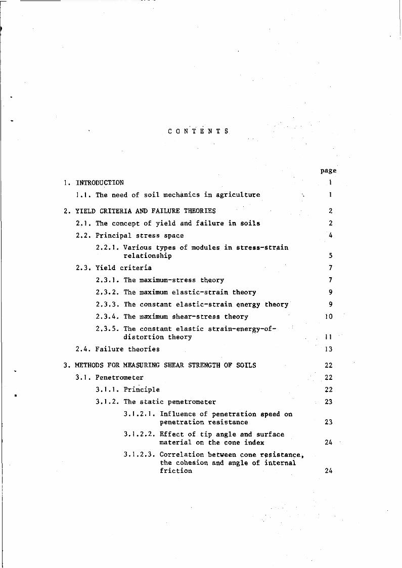
C O N T E N T S
page
1. INTRODUCTION 1
1.1. The need of soil mechanics in agriculture . 1
2. YIELD CRITERIA AND FAILURE THEORIES 2
2.1. The concept of yield and failure in soils 2
2.2. Principal stress space 4
2.2.1. Various types of modules in stress-strain
relationship 5
2.3. Yield criteria 7
2.3.1. The maximum-stress theory 7
2.3.2. The maximum elastic-strain theory 9
2.3.3. The constant elastic-strain energy theory 9
2.3.4. The maximum shear-stress theory 10 2.3.5. The constant elastic strain-energy-of-
distortion theory 11
2.4. Failure theories 13
3. METHODS FOR MEASURING SHEAR STRENGTH OF SOILS 22
3.1. Penetrometer 22
3.1.1. Principle 22
3.1.2. The static penetrometer 23
3.1.2.1. Influence of penetration speed on penetration resistance 23
3.1.2.2. Effect of tip angle and surface material on the cone index 24
3.1.2.3. Correlation between cone resistance, the cohesion and angle of internal friction 24

page
3.1.3. The dynamic penetrometer - Standard penetration test 27
3.1.3.1. Principle 27
3.1.3.2. Correlation between N-values of the standard penetration test and dynamic shear moduli 29
3.1.4. Summary 30
3.2. Vane-test 32
3.2.1. Principle 32
3.2.2. Influence of rate of loading on the vane
shear strength 35
3.3. Shear annulus 37
3.4. Solid shearhead 39
3.5. Direct shear test 41
3.6. Triaxial test 44
3.6.1. Types of triaxial test 44
3.6.2. Undrained test on saturated cohesive soils 45 3.6.3. Undrained test on partly saturated cohesive
soils 46
3.6.4. Consolidated-undrained test on saturated soils 47
3.6.5. Consolidated-undrained test on partly saturated soils 50
3.6.6. Drained tests 52
3.6.7. General remarks on the interrelationship of
the test results 52
3.7. Unconfined compression test 53
3.8. The different test procedures and their correlations 55
3.8.1. Correlations of cone resistance and vane shear strength for clays 55
3.8.2. Correlations of vane-test, unconfined compression test and undrained-unconsplidated triaxial test 56
3.8.3. Correlations of cone index, triaxial test and vane test 59
3.8.4. Comparison of methods of measuring soil shear strength using artificial soils 62
3.8.5. Schematic review of test correlations and literature cited 64
page
4. FRICTION ANGLE AND SHEAR STRENGTH OF COHESIONLESS SOILS 66
4.1. Definition of friction angle 66
4.2. Friction between minerals in granular form 66
4.3. Effect of surface water and surface roughness 68
4.4. Effect of normal load 71
4.5. Effect of confining stress on the shear strength 72
4.6. Effect of initial void ratio and density 72
4.7. Rate of loading 75
4.8. Vibrations and repeated loadings 76
4.9. Average particle size 76
4.10. Determination of in-situa friction angle 76
4.11. Summary. The choice of friction angle values for preliminary calculations 77
5. FRICTION ANGLE, COHESION AND SHEAR STRENGTH OF COHESIVE SOILS 80
5.1. Friction between sheet minerals 80
5:1.1. General nature of contact 80
5.1.2. Effect of soil moisture content on the friction angle 81
5.1.3. Effect of soil density on the friction angle 84
5.1.4. Correlation of drained friction angle and particle size distribution 85
5.1.5. Correlation of drained friction angle and plasticity index 86
5.2. Cohesion of clay soils 87
5.2.1. Cohesion and moisture content 87
5.2.2. Cohesion and soil density 88
5.3. Shear strength of cohesive soils 88
5.3.1. Difference between peak strength and ultimate strength 88
5.3.2. Peak strength and ultimate strength for soils with different clay content 90
5.3.3. Effect of soil moisture content on the shear strength 92
5.3.4. Physiochemical effects on the shear strength of clays 95

page
5.3.5. Influence of strain rate and confining pressure on the shear strength of compacted silt 98
5.3.6. Hyperbolic function to describe the stress-strain relation of compacted clays 99
5.3.7. Effect of consolidation on the drained shear strength of clays 105
5.3.8. Influence of soil density on the shear strength 107
5.3.9. Values of the c and $ (from undrained consolidated triaxial tests) 109
LITERATURE

1. INTRODUCTION
1.1. T h e n e e d o f s o i l m e c h a n i c s i n a g r i
c u l t u r e
The need of soil mechanics in agriculture is encountered in pro
blems such as compaction of the soil by agricultural machinery,
execution of drainage works, workability of the soil, traction per
formance of agricultural machines, bearing capacity of soils, con
dition of sport fields on different soils and under varying moisture
conditions.
In all these examples there are forces acting on the soil which
give rise to stresses and strains in the soil. In agriculture one is
interested in this stress-strain relationship in order to predict the
compaction of the soil after a certain activity in which the soil has
been exposed to forces produced by the wheight of heavy machinery.
For the evalution of traction performance one must know the maximum
shear strength of the soil.
There are different theories to describe the soil behaviour under
compression and or tension. We will treat several of these theories
which are called failure theories from which the Coulomb-Mohr failure
law is most commonly used (chapter 2).
The soil parameters such as shear strength and stress-strain
relationship etc. can be measured with several different test devices.
The different test devices do not always give the same values for the
soil parameters under investigation. Here an effort is made to give
an evaluation of these methods (chapter 3).
We will also indicate the most accurate test to investigate a
certain soil mechanical problem in agricultural engineering. The best

procedure to estimate the strength, compactibility etc. of the soil
is to run tests that duplicate the field conditions as closely as
possible, same degree of saturation, same total stress, and if pos
sible the same pressure in the liquid phase.
Because the values for the soil parameters of most common agri
cultural soils are not readily available in literature it was found
useful to collect these data and to indicate the influence of soil
density, moisture content and clay content on these parameters.
As the Coulomb-Mohr failure theory is used most widely at present
we give the value of c and <(> , the analytical cohesion and friction
angle respectively, and the shear strength for the most common soils
under different moisture and compaction conditions. These values have
been found in literature and were obtained with different test pro
cedures and sometimes not specified failure criteria and moisture
and density conditions (chapters 4 and 5). The accuracy of the values
is + 25% and one should use the values for preliminary calculations
only.
2. YIELD CRITERIA AND FAILURE THEORIES
2 . 1 . T h e c o n c e p t s o f y i e l d a n d f a i l u r e
i n s o i l s
The terms yield and failure cannot be applied indiscriminately
to soils. The failure of brittle materials, such as cast iron on
rock, occurs as a fracture with little or no plastic yielding. This
fracture can be readily identified with failure.
The term 'yield' in the field of plasticity is used to describe
the onset of plastic deformation, or, conversely, the upper limit
of elastic action (see fig. 2.1.).
The precise definition of yield in an actual material is related
to the characteristics of the stress-strain curve of the material;
only when there is a sharp break between the elastic portion (recove
rable deformation) and the plastic portion (non-recoverable defor
mation) of the stress-strain curve yield can be accurately defined.

Piecewise lineor
ff
B
A
C
**
D
E
E
Elastic-strain hardening (b) rnateriol
Elastic-perfectJy plastic 6
B
A
C
D
£
E
, . Rigid-linear hardening Rigid-perfectly plastic (e) (f)
Fig. 2.1. Typical stress-strain curves for various kinds of materials,
The yield stress
From YONG (1975)
The yield stress a occurs at point B in a-f•
In the fig. 2.1. a perfectly plastic material exhibits a conti
nued strain performance at the yield stress if the stress is sus
tained, as in fig. 2.1. d and f. The term plastic strain which is
commonly used denotes irrecoverable strain performance as in curve
BC in fig. 2.1. a. In this case, strain hardening is shown by BC.
The term fracture implies the appearance of distinct surfaces of
separations in the body, whereas yield is used to describe the onset
of plastic deformation with the resulting unrestricted plastic de
formation defined as flow. 'Failure' in a general sense includes
both fracture and flow. The curve DE shows what happens when the
compressive load is withdrawn and replaced by a tensile force.
2.2. P r i n c i p a l s t r e s s s p a c e
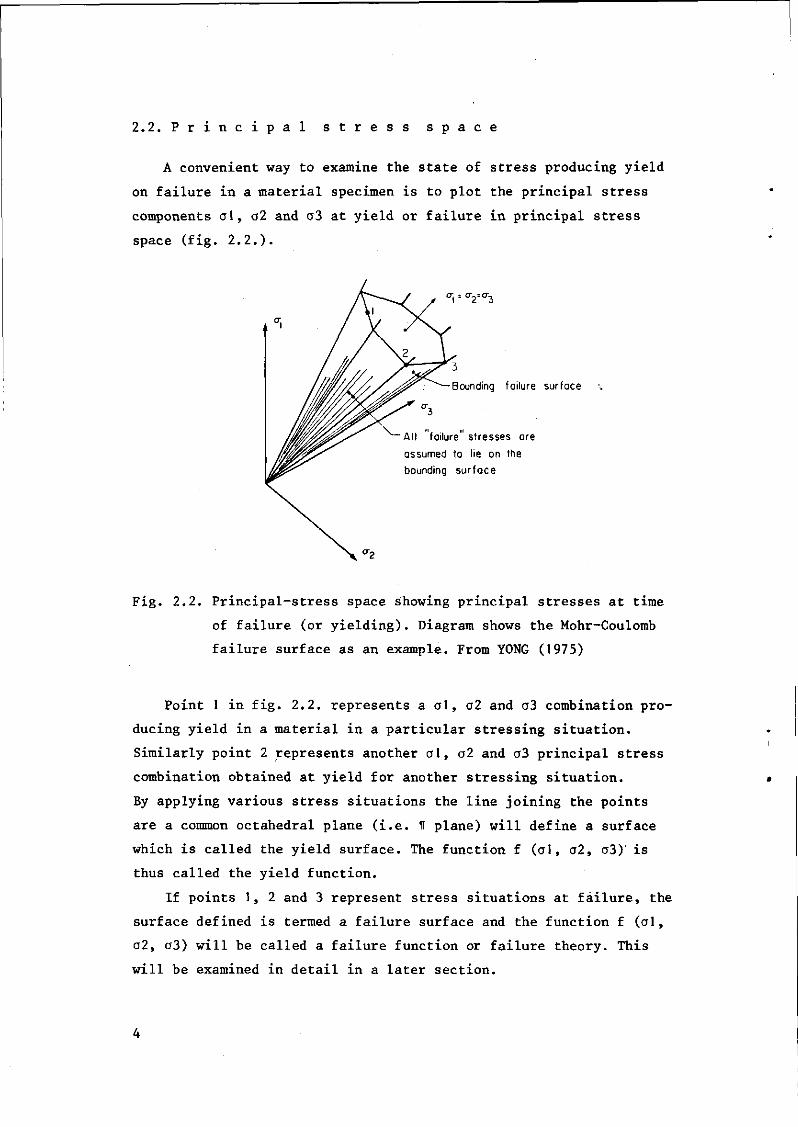
A convenient way to examine the state of stress producing yield
on failure in a material specimen is to plot the principal stress
components ol, a2 and a3 at yield or failure in principal stress
space (fig. 2.2.).
Bounding failure surface
All failure stresses are
assumed to lie on the
bounding surface
Fig. 2.2. Principal-stress space showing principal stresses at time
of failure (or yielding). Diagram shows the Mohr-Coulomb
failure surface as an example. From YONG (1975)
Point 1 in fig. 2.2. represents a ol, a2 and a3 combination pro
ducing yield in a material in a particular stressing situation.
Similarly point 2 represents another ol, a2 and a3 principal stress
combination obtained at yield for another stressing situation.
By applying various stress situations the line joining the points
are a common octahedral plane (i.e. U plane) will define a surface
which is called the yield surface. The function f (ol, a2, a3)' is
thus called the yield function.
If points 1, 2 and 3 represent stress situations at failure, the
surface defined is termed a failure surface and the function f (ol,
a2, a3) will be called a failure function or failure theory. This
will be examined in detail in a later section.

2.2.1. Various types of modules in stress-strain relationship
Concepts from the theory of elasticity
If we apply an uniaxial stress aZ to an elastic cylinder (fig.
2.3.) there will be a vertical compression and a lateral expansion
such that,
«"f (1) ex = ey = "y£Z
(2)
where
e , e , e = strains in the x, y, z directions, respectively
E = Young's modules of elasticity
y = Poisson's ratio
If shear stress xzix are applied to an elastic cube, there will be a
shear distortion such that
c „ T Z x I o \
f zx = -g— (3)
where three G = shear modules. Equations 1 to 3 define the three
basic constants of the theory of elasticity: E, G and y.
Actually only two of these constants are needed since
G - 27Ä7) <4)
For an elastic material with all stress components acting, we can
employ the principle of superposition to obtain:
1 ex = — {ax - y (ay+az)l (5a)
ey = Y -[ay - y (az+ax) } (5b)
e z = — 4 a z - y (ax+ay)\ (5c)
fxy - ̂ p (5d)
fyZ = ̂ (5e)
fzx = I ^ (5f )
the volumetric strain is
AV /c . — = ex + ex + ez (5g)
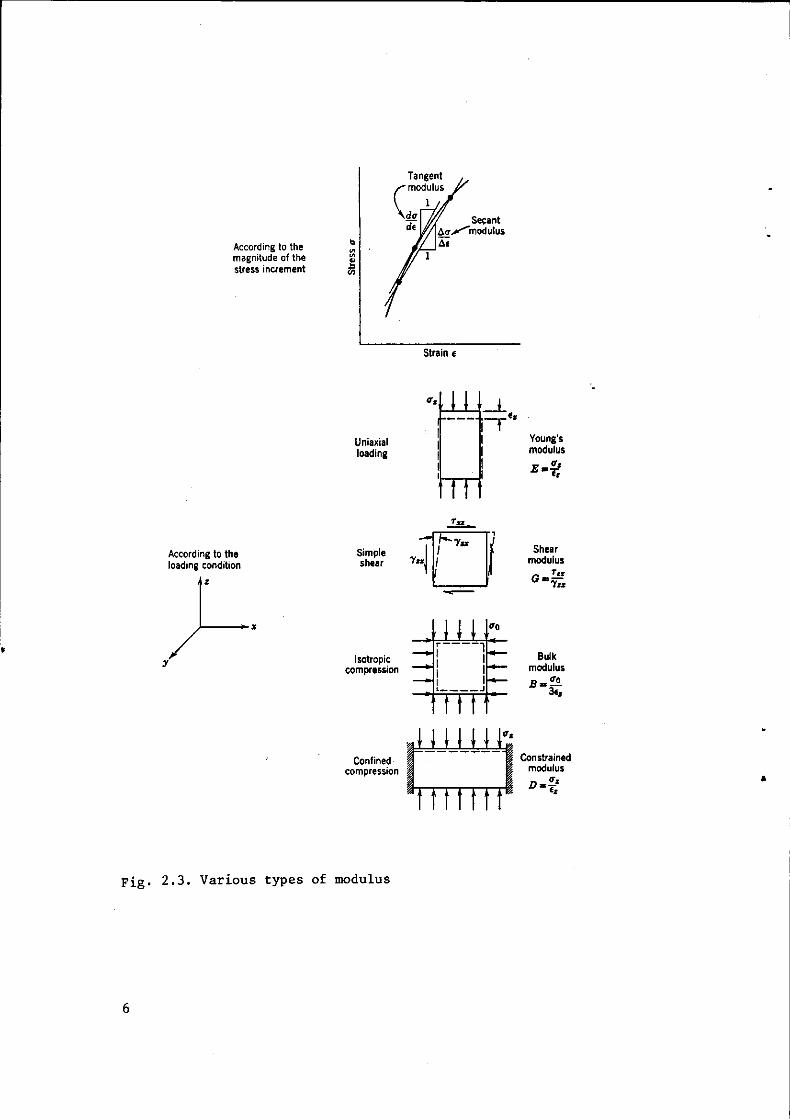
According to the magnitude of the stress increment
Tangent
(modulus 1
da Secant A2>^modulus Ac
Strain t
Uniaxial loading
' ' ' '
• 1 , .
\
i t 1 1 1 1 .
Young's modulus
According to the loading condition
Simple shear
Isotropic compression
T».
— » •
i •• i ' <r .
1 I
<T0
,
1 Confined |
compression %
I
I I " t " T T I T T I r/.
. 1 1 >
Shear modulus
r« Gm tix
Bulk modulus
B "35
1 Constrained I modulus
n _ _ » ^
Fig. 2.3. Various types of modulus
For the special case where ax=ay=az=ao and xxy=Tyz=Tzx=o the volume
change equals
AV 3ao ,. 0
The bulk modulus B is defined as
a AV/V 3(l-2y) (b)
Still another special type of modulus is the constrained modulus D
which is the ratio of axial stress to axial strain for confined
compression. This modulus can be computed from eq. (5) by setting
ex=ey=o.
Thus
ax = ay = -r—- az (7)
D _ E (1-y) (
- (l+y)0-2u) ( 8 )
Uniaxial loading and confined compression involve both shear strain
and volume change.
2.3. Y i e l d C r i t e r i a
2.3.1. The maximum-stress theory
The oldest theory of yielding and failure, sometimes known as
Rankine's theory, postulates that the maximum principal stress in
the material determines failure regardless of the magnitudes and
senses of the other two principal stresses. This gives rise to its
name "maximum-stress theory". Thus yielding in a stressed body in
accordance with this theory begins when the absolute value of the
maximum stress reaches the yield point stress of the material in
simple tension or compression.
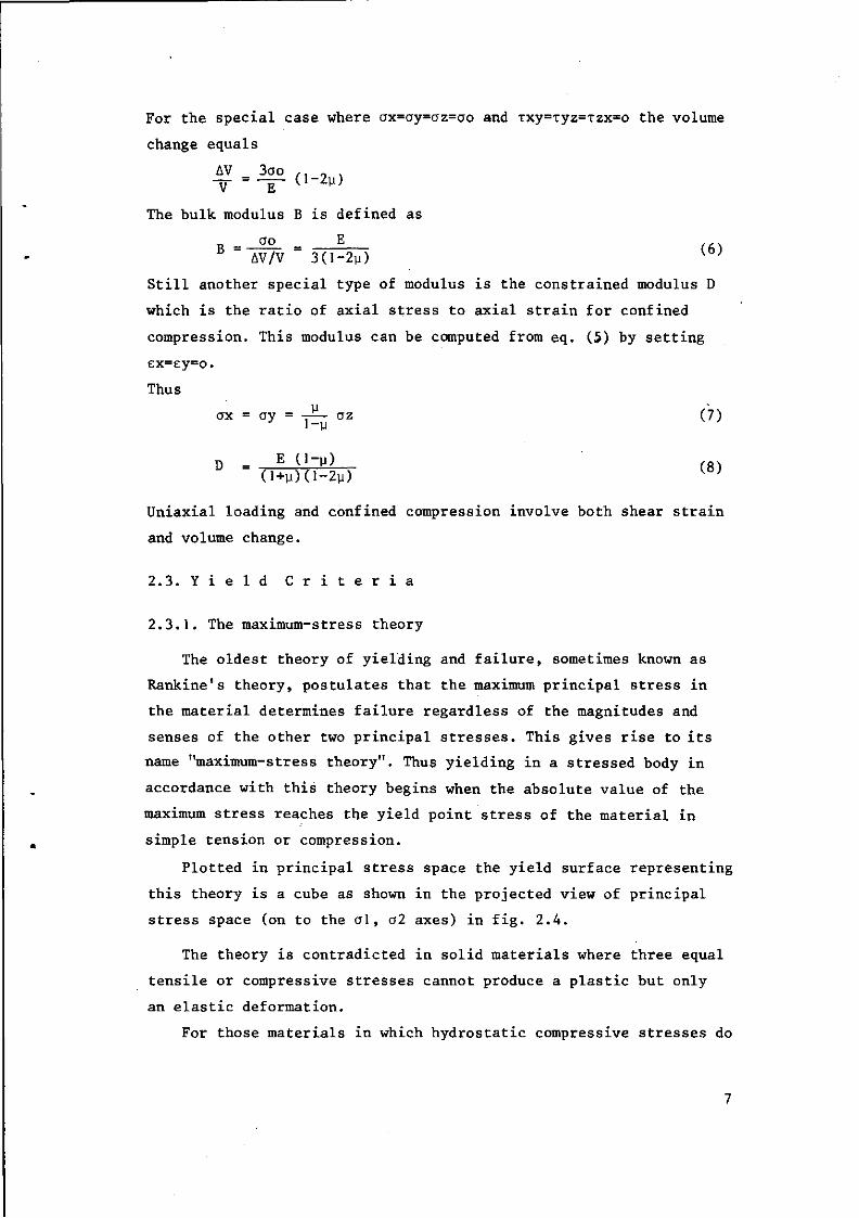
Plotted in principal stress space the yield surface representing
this theory is a cube as shown in the projected view of principal
stress space (on to the a\, a2 axes) in fig. 2.4.
The theory is contradicted in solid materials where three equal
tensile or compressive stresses cannot produce a plastic but only
an elastic deformation.
For those materials in which hydrostatic compressive stresses do

1234 = Maximum-stress theory ~ 5 6 7 8 = Maximum-strain theory •
A I B A ' 3 8 ' A = Maximum-sheor theory - Moximum-stroin-energy theory = Moximum-distortionol -energy theory
Material assumed to have same yield" point in tension and compression
Fig. 2.4. Representation of maximum shear-stress equation. (Timos-
henko, 1956, published by Van Nostrand-Reinhold Co., 1955
Litton Educational Publ. Inc.) from Yong, 1975
cause plastic deformation, the theory is contradited by the fact
that failure in simple tension in an isotropic material would be
along inclined planes on which neither the tensile nor compressive
stress is a maximum.
However, there is some merit in the theory when one considers
the strength of non-isotropic materials, particularly layered ma
terials, where there is a pronounced difference in strength proper
ties in different directions, e.g., a layered rock might have almost
no tensile strength in the direction normal to the layers and would
fail in tension by splitting along these layers.
The theory has also found some use in a modified form to explain
the cleavage fracture of crystals.
With these few exceptions the theory finds no application in
modern practice.

2.3.2. The maximum elastic-strain theory
The maximum elastic-strain theory, attributed to St. Venant,
assumes that a ductile material begins to yield when either the
maximum (elongation) strain equals the yield point strain in simple
tension, i.e.
£ i _ _ - L ( a 2 + a 3 ) - °y ^ n s i l e > (2.1.)
or the minimum (shortening) strain equals the yield point strain in
simple compression,
|°3-4(gï+a2)l = ay (co;Pressive> (2.2.)
where the principal stresses ol, a2 and o3 are considered positive
in tension, and are ordered such that a\>o2>a3 and u, E and ay are
Poisson's ratio, Young's modulus and yield point stress respectively.
In principal stress space the yield surface corresponding to
theory consists of two straight three-sided pyramids in inverted
positions relative to each other, having equilateral triangles as
sections normal to the axis which coincides with one of the space
diagonals, e.g. al=o~2=a3 (see fig. 2.4.)
The slopes of the sides of the pyramids would depend on Poisson's
ratio. This theory is again contradicted by material behaviour under
hydrostatic tensile or compressive stresses.
2.3.3. The constant elastic-strain energy theory
The quantity of strain energy per unit volume of the material
is used as the basis for determining failure in the constant elastic-
strain-energy theory. If we equate the strain energy for a given
state of stress at failure to the energy stored at yield in simple
tension the criterion may be written as:
2 ^|2 = _ L (al2+a22+o32) --H- (ala2+a2a3+a3al) (2.3.)
Again, the performance of materials under hydrostatic stresses
indicates that the elastic energy can have no significance as a li
miting condition.
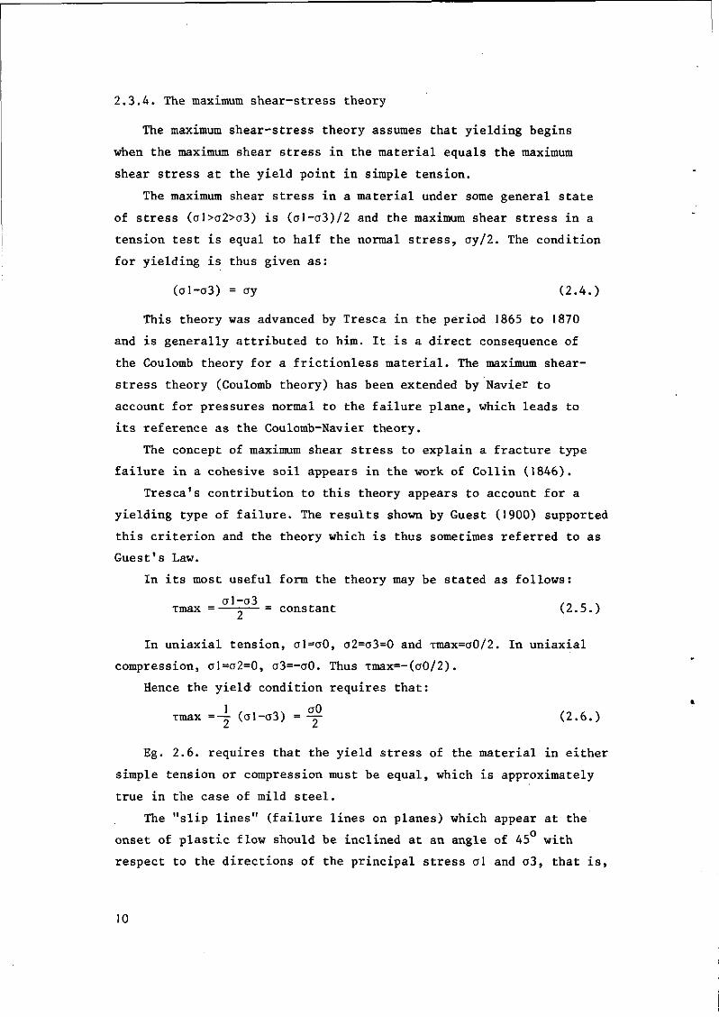
2.3.4. The maximum shear-stress theory
The maximum shear-stress theory assumes that yielding begins
when the maximum shear stress in the material equals the maximum
shear stress at the yield point in simple tension.
The maximum shear stress in a material under some general state
of stress (al>a2>a3) is (al-a3)/2 and the maximum shear stress in a
tension test is equal to half the normal stress, ay/2. The condition
for yielding is thus given as:
(al-a3) = ay (2.4.)
This theory was advanced by Tresca in the period 1865 to 1870
and is generally attributed to him. It is a direct consequence of
the Coulomb theory for a frictionless material. The maximum shear-
stress theory (Coulomb theory) has been extended by Navier to
account for pressures normal to the failure plane, which leads to
its reference as the Coulomb-Navier theory.
The concept of maximum shear stress to explain a fracture type
failure in a cohesive soil appears in the work of Collin (1846).
Tresca's contribution to this theory appears to account for a
yielding type of failure. The results shown by Guest (1900) supported
this criterion and the theory which is thus sometimes referred to as
Guest's Law.
In its most useful form the theory may be stated as follows:
xmax = r — = constant (2.5.)
In uniaxial tension, al=a0, a2=a3=0 and xmax=a0/2. In uniaxial
compression, al=a2=0, a3=-a0. Thus Tmax=-(a0/2).
Hence the yield condition requires that:
Tmax = — (al-a3) = -y (2.6.)
Eg. 2.6. requires that the yield stress of the material in either
simple tension or compression must be equal, which is approximately
true in the case of mild steel.
The "slip lines" (failure lines on planes) which appear at the
onset of plastic flow should be inclined at an angle of 45 with
respect to the directions of the principal stress al and a3, that is,
10
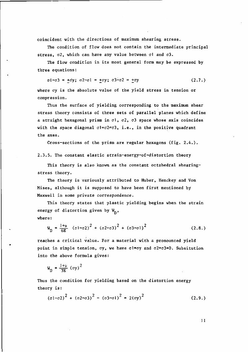
coincident with the directions of maximum shearing stress.
The condition of flow does not contain the intermediate principal
stress, a2, which can have any value between o\ and o3.
The flow condition in its most general form may be expressed by
three equations:
al-o-3 = +dy; a2-al = +ay; a3-a2 = +ay (2.7.)
where ay is the absolute value of the yield stress in tension or
compression.
Thus the surface of yielding corresponding to the maximum shear
stress theory consists of three sets of parallel planes which define
a straight hexagonal prism in o\, o2, a 3 space whose axis coincides
with the space diagonal al=a2=a3, i.e., in the positive quadrant
the axes.
Cross-sections of the prism are regular hexagons (fig. 2.4.).
2.3.5. The constant elastic strain-energy-of-distortion theory
This theory is also known as the constant octahedral shearing-
stress theory.
The theory is variously attributed to Huber, Henckey and Von
Mises, although it is supposed to have been first mentioned by
Maxwell in some private correspondence.
This theory states that plastic yielding begins when the strain
energy of distortion given by W ,
where :
Wn = ^S- (al-a2)2 + (a2-o-3)2 + (a3-al)2 (2.8.)
reaches a critical value. For a material with a pronounced yield
point in simple tension, ay, we have al=ay and a2=a3=0. Subsitution
into the above formula gives:
w D - ^ ( o y ) 2
Thus the condition for yielding based on the distortion energy
theory is :
(al-a2)2 + (a2-a3)2 - (a3-al)2 = 2(ay)2 (2.9.)
11

A useful form of the theory is obtained by passing a plane through
the unit points on the principal axes. Thus it is normal to a space
diagonal fig. 2.4. and 2.5. a\ , o2, cr3 space i.e., principal stress
space; there are thus eight such planes. The normal to each octahedral
plane has the direction cos (1//3) to each of the coordinate axes.
Normal and shearing stresses on the octahedral plane are called
"octahedral stresses".
Compression envelope
Spoce diagonal
Extension envelope
J2«y
Fig. 2.5. Failure envelopes from Yong, 1975
Thus the normal octahedral stress, aoct, is:
aoct = -j- (al+a2+a3) =̂ --Jl (2.10.)
where Jl = al+a2+o3 = first stress invariant
The octahedral shearing stress is:
aoct = ~ {(o\-a2)2 + (a2-a3)2 + (a3-al)2t 2 {< V (2.11.)
Thus any state of stress consisting of three principal stresses
may be resolved into two component states of stress,
12

a) a component consisting of equal tensile (or compressive) stresses
acting in all directions, and
b) a component state of stress consisting of the eight octahedral
shearing stresses.
Thus from egs. 2.9 and 2.11
9(aoct)2 = 2(ay)2
and hence:
/2 aoct =—J- ay (2.12)
Eq. 2.12 is thus a statement of the maximum energy of distortion
theory. The theory further shows that at the plastic limit the
octahedral shearing stress in the material is constant, which de
pends on the yield point of the material in simple tension or
compression. The yield stresses in simple tension and compression
are thus assumed to be equal.
The yielding surface defined by this theory is a straight cir
cular cylinder whose axis coincides with the space diagonal al=o2=a3.
Since planes normal to the axis of the cylinder are octahedral
planes, the radius of the cylinder equals the octahedral shearing
stress. The radius of the cylinder is therefore /2/3 ay. This is
similar to the Von Mises yield criterion.
2.4. F a i l u r e t h e o r i e s
The failure theory proposed by MOHR (1900) followed the earlier
work of Coulomb and Navier which considered the state of failure as
a shear failure. As it turns out, both the Coulomb-Navier theory and
the extended maximum shear-stress theory are special cases of the
Mohr theory.
The theory which considers failure by both yielding and fracture
(assuming slippage as a mode of failure) provides a functional re
lationship between normal and shear stresses on the failure plane,
i.e.
r= f(a)
13

.where T = shearing stress along the failure plane
a = normal stress across the failure plane.
From the two-parameter nature of the theory the curve defined
by this functional relationship may be plotted on the T, a-plane
(fig. 2.6).
Pf
l
I \ Direction C. .-of failure
/ ' plane
/
Envelope drawn tangent to experimental curves
T,,-f[
Mohr rupture envelope
^Experimental stress circle
Fig. 2.6. Mohr's failure theory plotted in the T-a plane from Yong,
1975
Since changing the sign of T merely changes the direction of
failure but not the condition for it, the curve must be symmetrical
about the a-axis. The curve so obtained which is termed the Mohr
rupture envelope, represents the locus of all points defining the
limiting values of both components of stress (r and a) in the slop
planes under the different states of stress al, a2, a3 to. which
the material may be subjected.
The Mohr envelope thus reflects a property of the material
which is independent of the stresses imposed on the material.
The theory is attractive for use in studying the shear strength
14

of soils since there is no requirement that the material obeys Hooke's
law (for ideal elastic material) or that Poisson's ratio be constant:
also, the strength and stiffness of the material in tension and com
pression need not to be equal.
The Coulomb equation, r=c+a tan $ , represents a special case of
the Mohr theory of strength in which the Mohr envelope is a straight
line inclined to the normal stress axis at angle cf.
The use of the Coulomb equation to represent the Mohr envelope
in the Mohr diagram is called the Mohr-Coulomb theory.
Mohr's hypothesis states that failure depends upon the stresses
on the slip planes and failure will take place when the obliquity
of the resultant stress exceeds a certain maximum value.
It is also stated that "the elastic limit and the ultimate
strength of materials are dependent on the stresses acting on the
slip planes".
The Mohr representation of stresses acting on the three principal
planes is shown in fig. 2.7.
Fig. 2.7. Mohr representation of stresses in three-dimensional system
from Yong, 1975
15

Stresses on any plane within the body must be within the shaded
area. The slope of the line joining the origin and point A gives the
obliquity of stress. The maximum inclination of stress will be given
by the targets to the largest circle.
Failure occurs on planes where stresses are represented by points
B and C. These stresses act on planes which are parallel to the dia
meter of the intermediate principle stress. Therefore the diameter
of the largest Mohr circle and the magnitude of the stresses at points
B and C are independent of the intermediate principal stress, a2.
With the assumption that al is the intermediate principal stress,
the largest of three circles representing the limiting state of
stress will be of diameters (al-a3) and centred at (ol+o3)/2 along
the a-axis, as seen in fig. 2.6, taking due account of the algebraic
sign of the stresses. Since the two parallel sets of slip planes
which occur when an isotropic specimen has been stressed slightly
beyond the plastic limit by a state of homogeneous stress are sym
metrically inclined with respect to the directions in which the major
and minor principal stresses act, and the two plane systems intersect
each other along the direction in which the intermediate principal
stress acts, Mohr assumed that the intermediate principal stress is
without influence on the failure of a material.
Accordingly, some point on the perimeter of the circle of dia
meter (al-03) must represent the limiting stress condition.
The theory thus affords a method of devising a failure theory
for a specific material, i.e., establishing its Mohr rupture envelope,
from actual test results.
In practice a series of similar specimens is subjected to dif
ferent stresses and brought to failure (as in the triaxial test).
The various Mohr's stress circles are plotted for the limiting
states of stress and the unique failure stress on the failure plane
for each test is taken as the point of common tangency between a
smooth limiting curve (or envelope) and the various (al-o3) circles.
By taking the points of common tangency as representative of
the a and r stresses on the failure plane, a state of homogeneous
stress in an isotropic material is assumed. Due to experimental
16

shortcomings, however, one may not necessarily obtain a state of
homogeneous stress and thus the inferred stresses at the point of
common tangency for the envelope, obtained experimentally, will not
in all likelihood represent the actual stresses on the failure plane.
It follows then that the predicted location of the failure plane,
based on the common tangency points might be in error.
The possible discrepancy between the actual Mohr rupture envelope
and an experimentally obtained envelope is shown on fig. 2.6.
Actual Mohr rupture envelopes are often curves. However, for
soils the curvature is usually not great and it has proved useful to
approximate the envelope by a straight line, at least over a limited
range of normal stress.
The equation of a straight line in the T, a-plarie is the Coulomb
equation r=S=C+a tan <f>,.
From fig. 2.8. the following formula may be derived:
D o1-a3 ,al+à3. . R = — ~ — = c cos <}> + (—-—Jsin $
(2.13)
Fig. 2.8. Properties of a straight-line Mohr envelope, a\ and a3 are
limiting effective stresses at failure. Compressive stresses
considered positive in deriving eg. 8.13. from Yong, 1975
17
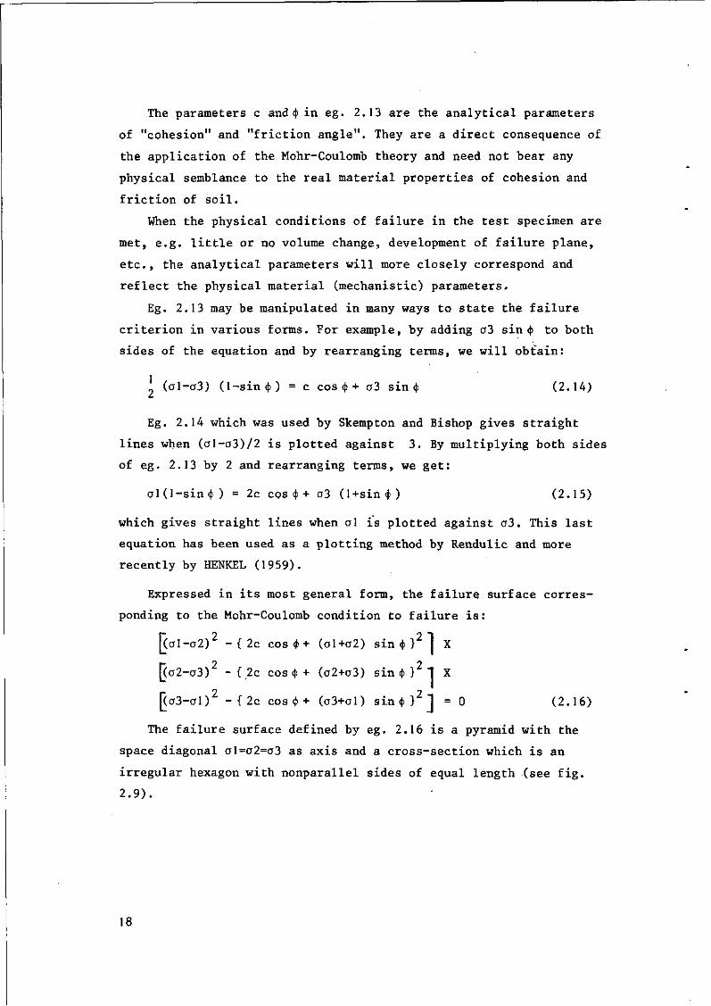
The parameters c and $ in eg. 2.13 are the analytical parameters
of "cohesion" and "friction angle". They are a direct consequence of
the application of the Mohr-Coulomb theory and need not bear any
physical semblance to the real material properties of cohesion and
friction of soil.
When the physical conditions of failure in the test specimen are
met, e.g. little or no volume change, development of failure plane,
etc., the analytical parameters will more closely correspond and
reflect the physical material (mechanistic) parameters.
Eg. 2.13 may be manipulated in many ways to state the failure
criterion in various forms. For example, by adding a3 sin c(> to both
sides of the equation and by rearranging terms, we will obtain:
. (al-a3) (l-sin<(>) = c cos <j> + o3 sin $ (2.14)
Eg. 2.14 which was used by Skempton and Bishop gives straight
lines when (al-a3)/2 is plotted against 3. By multiplying both sides
of eg. 2.13 by 2 and rearranging terms, we get:
al(l-sin<(;) = 2c cos $ + a3 (l+sin<f>) (2.15)
which gives straight lines when al is plotted against cr3. This last
equation has been used as a plotting method by Rendulic and more
recently by HENKEL (1959).
Expressed in its most general form, the failure surface corres
ponding to the Mohr-Coulomb condition to failure is:
[(oi-a2) -{2c cos(|>+ (oi+a2) sin 4> } 2 j X
[(a2-a3)2 -{.2c cos $ + (a2+a3) sin <f> } 2 1 X
j ( a 3 - a l ) 2 - { 2 c cos <|> + (a3+al) s in<|>}21 = 0 (2 .16)
The failure surface defined by eg. 2.16 is a pyramid with the
space diagonal al=a2=a3 as axis and a cross-section which is an
irregular hexagon with nonparallel sides of equal length (see fig.
2.9).
18

Mohr-Coulomb
TT Plane
so tropic line
°5 = Constant plane Stress paths in conventional triQxial tests
Failure locus
Fig. 2.9. Mohr-Coulomb failure surface in principal stress space
showing stress paths in conventional triaxial tests,
(from YONG, 1975)
The projection of this irregular hexagon on the plane al+a2+o3 =
constant (i.e. a plane at night angles to the space diagonal or an
octahedral plane) is shown in fig. 2.10. The three criteria are seen
to coincide for compressive tests but the strength in a tensile test
is seen to be less for the Mohr-Coulomb failure theory.
19

Extended von Mises
/ . Extended Tresca
Mohr -Coulomb
Projection on plane
Fig. 2.10. Failure surfaces-Mohr Coulomb and extended yield criteria,
(from YONG, 1975)
More details about soil behaviour and failure laws can be found
in the work of SCHOFIELD (1968) and KURTAY (1970).
20
LITERATURE CHAPTER 2.
KURTAY, T. and A.R. REECE, 1970. Plasticity theory and critical
state soil mechanics. Journal of Terramechanics, Vol. 7,
nos. 3 and 4. pp 23 to 56. Pergamon Press., Printed in
Great Britain.
LAMBE T. WILLIAM and ROBERT V. WHITMAN, 1969. Soil Mechanics -
Massachusetts Institute of Technology. John Wiley and Sons
Inc. New York.
SCHOFIELD, ANDREW and PETER WROTH, 1968. Critical State Soil Mecha
nics. Mc. Graw-Hill. London
YONG, R.N. and B.P. WANKENTIN, 1975. Soil Properties and Behaviour.
Developments in Geotechnical engineering. Vol. 5 - Elsevier
Scientific Publishing Company.
21
3. METHODS FOR MEASURING SHEAR STRENGTH OF SOILS
3.1. P e n e t r o m e t e r
3.1.1. Principle
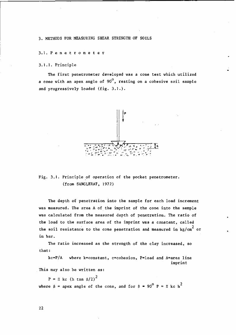
The first penetrometer developed was a cone test which utilized
a cone with an apex angle of 90 , resting on a cohesive soil sample
and progressively loaded (fig. 3.1.).
1/ ,1 • /// //
Fig. 3.1. Principle of operation of the pocket penetrometer,
(from SANGLERAT, 1972)
The depth of penetration into the sample for each load increment
was measured. The area A of the imprint of the cone into the sample
was calculated from the measured depth of penetration. The ratio of
the load to the surface area of the imprint was a constant, called 2
the soil resistance to the cone penetration and measured in kg/cm or
in bar.
The ratio increased as the strength of the clay increased, so
that:
kc=P/A where k=constant, c=cohesion, P=load and A=area line
imprint
This may also be written as:
2
2
P = n kc (h tan ß/2)'
where ß = apex angle of the cone, and for ß = 90 P = II kc h
22

From experimental data, it is possible to determine the value of
the constant k, and once it is known, cohesion c may be obtained.
3.1.2. The static penetrometer
Here the cone is driven into the soil with a constant speed and
the resistance to penetration i6 measured.
3.1.2.1. I n f l u e n c e o f p e n e t r a t i o n s p e e d
o n p e n e t r a t i o n r e s i s t a n c e . On clay the in
fluence 01 the penetration speed has a considerable influence on the
penetration resistance. FREITAG (1968) found a relationship between
strength ratio and penetration speed as shown in fig. 3.2., where
the strength ratio is the soil strength measured at a speed of 180
cm/min devided by the strength at actual speed.
500 1000 1500 2000 penetration speed cm/min
Fig. 3.2. Strength ratio versus penetration speed from FREITAG (1968)
Normally the penetration speed is less than + 50 cm/min in
research measurements and the influence of different penetration
speed is negliable.
However one should prefer a mechanical operated penetrometer
which is driven into the soil at a constant speed and where the
resistance is registrated automatically.
23

3 . 1 . 2 . 2 . E f f e c t - o f t i p a n g l e a n d s u r f a c e
m a t e r i a l o n t h e c o n e i n d e x . GILL (1968) found
an in f luence of the t i p angle of the cone on the cone index (pene
t r a t i o n - r e s i s t a n c e force devided by the maximum c ross s e c t i ona l a rea
of the penetrometer t i p ) f i g . 3 . 3 .
kg /cm 2 CONGAREE soil 200r 14.1
MOLOKAI SOil DECATUR Soi l
I50-
z IOO-7,
50
I0 20 30 40 50 60 0 I0 20 30 40 50 60 O I0 20 30 40 50 60 TIP ANGLE <0)
X TEFLON CONE
Fig. 3.3. Effect of tip angle and surface material on cone index
from GILL, 1968
The U.S. Army Waterways Experiment Station at Vicksburg, Miss,
reported data to show that tip shape had little influence on the
cone index values of soils. In U.S. the constante-rate type of soil
penetrometer with tip angle of 30 and maximum surface area of 0.5
sq. in- is often used. In Europe a cone with a tip angle of 60 and 2 a maximum surface area of 10 cm is more common.
One must always be aware of the difference between friction
on the shaft and the resistance to the cone itself when the values
of two different types of penetrometers are compared.
3 . 1 . 2 . 3 . C o r r e l a t i o n b e t w e e n c o n e r e s i s
t a n c e , t h e c o h e s i o n a n d a n g l e o f i n t e r
n a l f r i c t i o n . In a g r i c u l t u r a l s o i l mechanical problems we
a r e mostly i n t e r e s t e d in the f i r s t 2 or 3 meters of the s o i l . There-
24

fore the de Beer theory for the interpretation of penetrometer test
data for shallow foundations may be of interest.
The de Beer theory is based on the formulas derived by
K. Buisman of the Delft Laboratory of soil mechanics which, in turn,
were derived from the Prandtl-Caquot equations (SANGLERAT, 1972).
For practical purposes the resistance at the point of the pene
trometer could be expressed by the following equation (from experi
mental data of Keverling Buisman, Delft)
[ 2 'Il <k n tan* c r 2 .II <k H tan* ,-, po tan2 (J+|) e + t £ m ^{ tan (4+J) e * - 1}J
eg. 1
where qc = cone resistance
po = overburden pressure at the same level of the cone.
The empirical coefficient of 1.3 is due to the conical shape of
the penetrometer point (10.0 - cm section, apex angle of 60 ).
When dealing with sands, c=o and knowing the value of qc, the angle
of internal friction may be calculated from equation 1 .
When dealing with homogeneous cohesive material, the value of
qc must be determined at two locations at different depths. This
gives a set of two equations with two unknowns, namely, the cohesion
c and the angle of shearing resistance*. These two unknowns can
theoretically be calculated. De Beer has produced practical calcu
lation methods for the solution of the equations.
Other practical values for the cohesion of normally consolidated
sandy clay are between qc/10 and qc/20, depending on the type of
penetrometer used.
From Sanglerat page 201,
"It has been shown here how important it is to know the type of
penetrometer used in field tests to determine by which formula
the cohesion may be evaluated".
For deeper penetration tests de failure surface above and below
the cone is very similar tot that presented in fig. 3.4.
25

Fig. 3.4. Critical embedment: logarithmic spiral equation Y> = d ß tan <j>
Y = d e from SANGLERAT (1972)
The print resistance is actually equal to twice the value ob
tained from the Buisman-Prandtl formula (eq. 1 ) . It can therefore
be concluded that the failures occuring both above and below the
point each contribute about 50% of the resistance of penetration
of the cone.
For cohesive soils <(> = 0 one has found the formula
cu = (qc - Pb) / 13,4
where qc = priot resistance of the penetrometer in bar
cu = cohesion
Pb = overburden pressure at the depth of the test.
At shallow depths, the value of Pb is often so small that it may
be ignored.
The coefficient of 13.4 used with the data of the penetrometer
tests gives results which are in very good agreement with those of
the vane shear tests.
26
3.1.3. The dynamic penetrometer - Standard Penetration test
3.1.3.1. P r i n c i p l e . The most widely used penetration test
is the "standard penetration test", which consists of driving a
spoon into the ground by dropping a 63,4 kg weight from a height of
0,76 m (LAMBE and WHITMAN, 1969).
The penetration resistance is reported in number of blows of the
weight to drive the spoon 0,3 m.
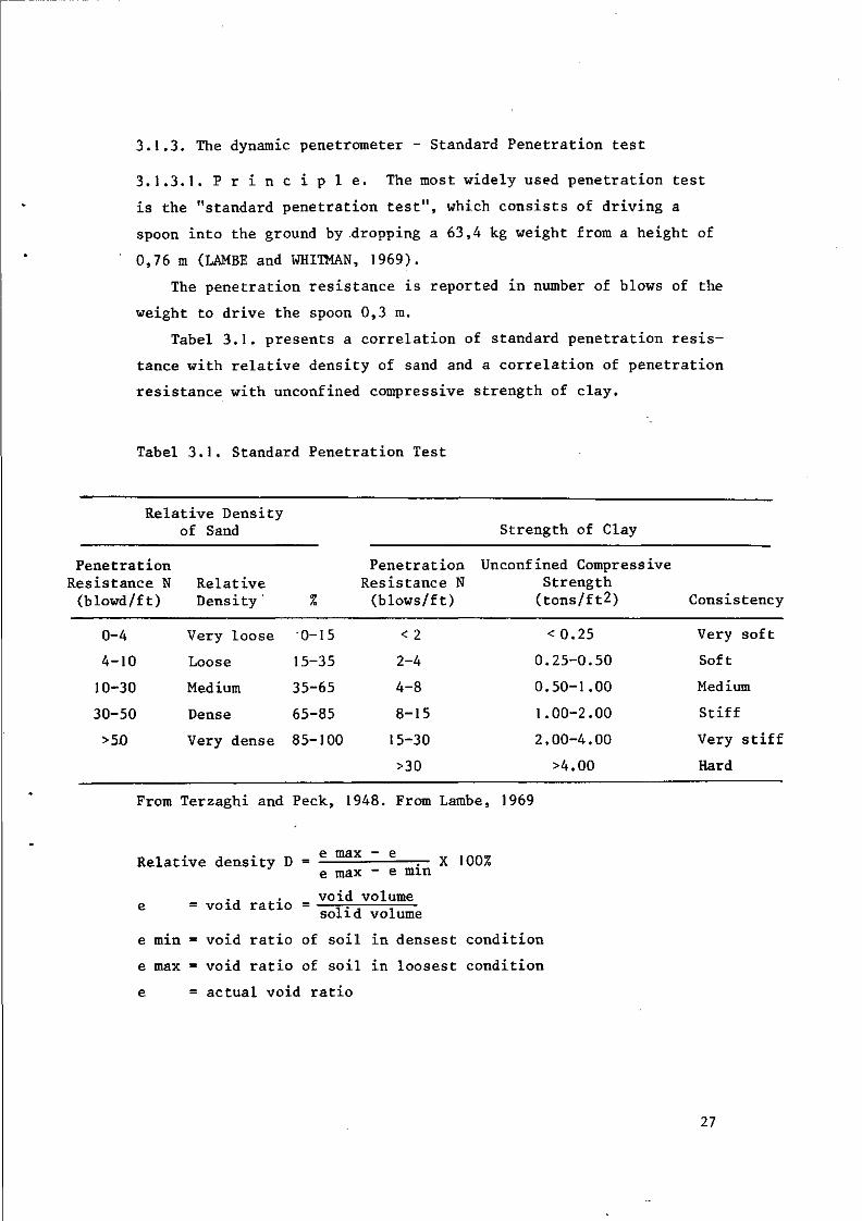
Tabel 3.1. presents a correlation of standard penetration resis
tance with relative density of sand and a correlation of penetration
resistance with unconfined compressive strength of clay.
Tabel 3.1. Standard Penetration Test
Relative Density of Sand Strength of Clay
Penetration Resistance N Relative
(blowd/ft) Density '
Penetration Unconfined Compressive Resistance N Strength
(blows/ft) (tons/ft2) Consistency
0-4 Very loose 0-15
4-10 Loose 15-35
10-30 Medium 35-65
30-50 Dense 65-85
>5J0 Very dense 85-100
< 2
2-4
4-8
8-15
15-30
>30
<0.25
0.25-0.50
0.50-1.00
1.00-2.00
2.00-4.00
>4.00
Very soft
Soft
Med ium
Stiff
Very stiff
Hard
From Terzaghi and Peck, 1948. From Lambe, 1969
Relative density D =
e = void ratio =
e max - e e max - e min
void volume
X 100%
solid volume
e min = void ratio of soil in densest condition
e max = void ratio of soil in loosest condition
e = actual void ratio
27
The standard penetration test is a very valuable method of soil
investigation. It should, however, be used only as a quide, because
there are many reasons why the results are only approximate.
As laboratory tests show the penetration resistance depends on
factors other than relative density. The penetration resistance
depends on the confining stress and or the type of sand. The in
fluence of sand type on penetration resistance is particularly large
at low densities.
Another factor that may have a marked influence on the penetra
tion resistance in a sand is the pore pressure condition during the
measuring operation.
Experience has shown that the determination of shear strength
of a clay from the penetration test can be very unreliable (LAMBE
and WHITMAN, 1969).
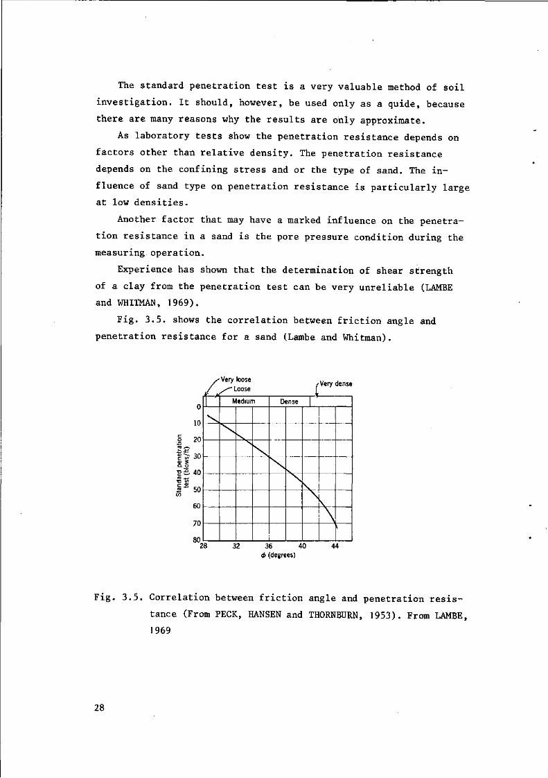
Fig. 3.5. shows the correlation between friction angle and
penetration resistance for a sand (Lambe and Whitman).
0
10
•I 20
f § 30 CD 5 Q. o T3-Q. An
Sta
ndar
te
st(
3 o
c
70
Rfl
.^Very loose
/ ^ L o o s e
Medium Dense
s. -
( Very dense
28 32 36 40 <t> (degrees)
44
Fig. 3.5. Correlation between friction angle and penetration resis
tance (From PECK, HANSEN and THORNBURN, 1953). From LAMBE,
1969
28

3 . 1 . 3 . 2 . C o r r e l a t i o n b e t w e e n N - v a l u e s o f
t h e s t a n d a r d p e n e t r a t i o n t e s t a n d d y
n a m i c s h e a r m o d u l i . Dynamic shear modulus i s one of
the most important parameters in the response ana lyses of s o i l d e
p o s i t s dur ing an ea r thquake .
Because the standard penetration test is a simple and rapid
means of soil exploration, extensive efforts have been made to cor
relate the results of the test with a number of important soil pro
perties which otherwise require laborious sampling and testing tech
niques for their determinations.
OHSAKI and IRVASAKI (1973) report that from statistical analyses
of accumulated data on dynamic characteristics of various soil de
posits measured by means of seismic exploration it has been found
that shear moduli for small shear strain level are well correlated
with N-values of the standard penetration test, and that their in
terrelation may be expressed by a simple, approximate eg.
G = 1200 N0'8 (tons/sq. meter)
where :
G = shear modulus
N = n-values of the standard penetration test (blows/ft)
OHTA ET ALL (1972) found G = 1390 N°' 7 2
They found for different soils different correlation coefficients
and other values for the coefficients (see fig. 3.6).
29

50000
ÏOCOG
5000
1000
500
i
i o
• S* 'S s r sr
S (
! 1 ' 1 • !
G - 13
1 1
1 y
V
! ' i i i l ! ' '
I l i ; i l 1 1 ! i 1 .
S O N 0 - ' 2
1 i !
1 ! | i W 1 «
\ "? / V i
l
j 1 1 1
' *
1 I É
i ! ' |
j . •• x -
•
n |i
' A
9
; ! '— •• n
^r !?r^ 0
IS* 1 $ <
* Vf, " f rM : ! > ' . . ' u
V*r y À
\ .1 1 1"
< ' I
I !
»Y
•J " ' *
^
j
i
0
LJ-f
4 TERTIARY SOIL o DILUVIAL SANDY SOIL
o AM IIVTAI CANDV M Ï I • ~ "
•r e
_ .
COHESIVE SOIL
•Mil l 0.5 5 10
N-VALUE
50 100
Fig. 3.6. Shear moduli and N-values (OHTA ET AL, 1972) from OHSAKI,
1973
Relationships between Poisson's ratio and shear modulus under
dynamic and static conditions have also been pointed out by Ohsaki
and Iwasaki.
3.1.4. Summary
In present publications the principal approach encountered is
to relate the penetrometer resistance for a certain type of soil
on a specific location with the cohesion and angle of internal
friction or other soil mechanical parameters which are determined
with other measuring devices (i.e. uniaxial tests, unconfined com
pression test, vane tests, shear tests).
This for the sake of rapideness and cheapness of the penetrometer
test compared with the other tests.
For static soil mechanical parameters the static penetrometer is
preferable above the dynamic penetrometer because of the lack of
theoretical background for the dynamic penetrometer.
For dynamic soil mechanical parameters one can use the dynamic
penetrometer as showed OHSAKI (1973).
30

LITERATURE PENETROMETER CHAPTER 3.1.
FREITAG, H.R., 1968. Penetration tests for Soil Measurements Trans
actions of the ASAE, vol. 11 no. 6, pp. 750-753.
GILL, WILLIAM R., 1968. Influence of compaction hardening of Soil on
Penetration Resistance. Transactions of the ASAE vol 11. no.
6, pp. 741-745.
LAMBE, T. WILLIAM and ROBERT V. WHITMAN, 1969. Soil Mechanics -
John Wiley and Sons, Inc. London.
OHSAKI, YONIHIKO and RYOJI IWASAKI, 1973. On dynamic shear moduli
and Poisson's ratio's of soil deposits - Soils and Foundations.
Vol. 13 no. 4, dec. 1973.
SANGLERAT, G, 1972. The penetrometer and soil exploration. Elsevier
Scientific Publishing Company, Amsterdam.
31
3 .2 . V a n e t e s t
3 . 2 . 1 . P r i n c i p l e
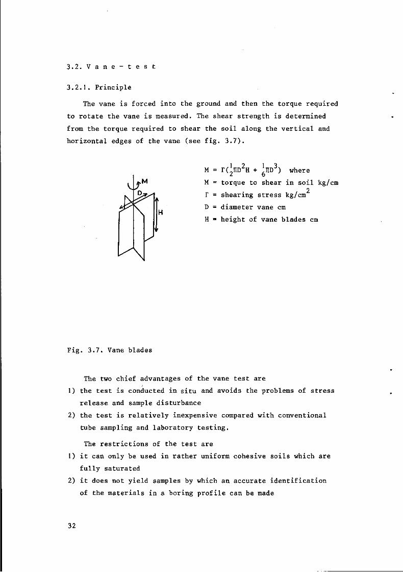
The vane is forced into the ground and then the torque required
to rotate the vane is measured. The shear strength is determined
from the torque required to shear the soil along the vertical and
horizontal edges of the vane (see fig. 3.7).
^ M
H
M = r(2lID2H + ^IID3) where
M = torque to shear in soil kg/cm 2
r = shearing stress kg/cm
D = diameter vane cm
H = height of vane blades cm
Fig. 3.7. Vane blades
The two chief advantages of the vane test are
1) the test is conducted in situ and avoids the problems of stress
release and sample disturbance
2) the test is relatively inexpensive compared with conventional
tube sampling and laboratory testing.
The restrictions of the test are
1) it can only be used in rather uniform cohesive soils which are
fully saturated
2) it does not yield samples by which an accurate identification
of the materials in a boring profile can be made
32

3) it imposes a failure surface on the soil which may not be rele
vant to the problem being studied (EDEN, 1966)
4) inserting the vane into the soil disturbs the soil or the "un
disturbed sample".
With the vane test one cannot apply a normal load to the soil.
So the shear strength is only measured with normal zero, hence one
cannot distinguish between cohesion and friction components in the
shear strength formula.
Therefore the vane test is only used in cohesive soils wittig
supposed to be zero and so the shear strength is completely due to
the cohesion.
Fig. 3.8. gives different types of vanes.
33

A—standard vane, 0 to 1.0 ton/ft2 range B—high-capacity vane adapter, 0 to 2.5 ton/ft2 range C—sensitive vane adapter, 0 to 0.2 ton/ft2 range
Acorn nut
Calibrated dial number plate—-f Stop pin
Snap ring Insert
Spacer
Teflon washer
Handle
3 Teflon washers (.020 thick) 6-32 Set screw
Spring
/4"-20 Socket head cap screw
6-32 Set screw
Shear vane
Fig. 3.8. Hand-operated torsional vane shear device from SIBLEY
(1966)
34

3.2.2. Influence of rate of loading on the vane shear strength
SIBLEY (1966) found the relationship between shear strength and
rate of stress as showed in fig. 3.9.
1.20
1.00
or
0.80
LU
et
0.60
i CO
0.40
Sv,
Sy*o Sv,
Sv20 Sv,
0 ^ * o - o 3 n "
,-^f T A
B"
„
0.20 0.40 0.60 VANE SHEAR STRENGTH SV| in tons/sq.ft.
0.80
X 0.I95
-L.
k g / c m
LEGEND
Sv - Vane shear strength, rate of stress approx. O.I tsf/second
o Sv5 - Vane shear strength, rate of stress = O.I t s f / 5 seconds
a S V | 0 '
Vane shear strength, rate of stress O.I tsf/IOseconds A Sv - Vane shear strength, rate of stress = O.I t s f / 20 seconds
Fig. 3.9. Relationship between torsional vane shear strength and
rate of stress, Bootlegger Cove clay (from SIBLEY, 1966)
A high loading rate gives a higher strength especially in soils
with a low shear strength.
35

LITERATURE VANE TEST CHAPTER 3.2.
EDEN, W.J. An evaluation of the field vane test in sensitive clay.
Vane shear and Cone Penetration Resistance Testing of In-
Situ Soils, ASTM STP 399, Am. Soc. Testing Mats. 1966, p.8.
SIBLEY, E.A. and G. YAMANE. A simple shear test for saturated co
hesive soils. Vane shear and cone penetration resistance
testing of in-situ soils, ASTM. STP 399, Am. Soc. Testing
Mats. 1966, p.39.
36
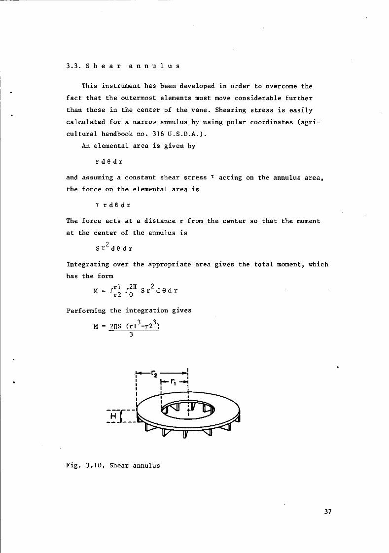
3.3. S h e a r a n n u l u s
This instrument has been developed in order to overcome the
fact that the outermost elements must move considerable further
than those in the center of the vane. Shearing stress is easily
calculated for a narrow annulus by using polar coordinates (agri
cultural handbook no. 316 U.S.D.A.).
An elemental area is given by
r de dr
and assuming a constant shear stress T acting on the annulus area,
the force on the elemental area is
T rdedr
The force acts at a distance r from the center so that the moment
at the center of the annulus is
Sr2d6 dr
Integrating over the appropriate area gives the total moment, which
has the form
M = ;rI fln S r2 d 0 d r r2 0
Performing the integration gives
M = 2nS (rl3-r23)
Fig. 3.10. Shear annulus
37
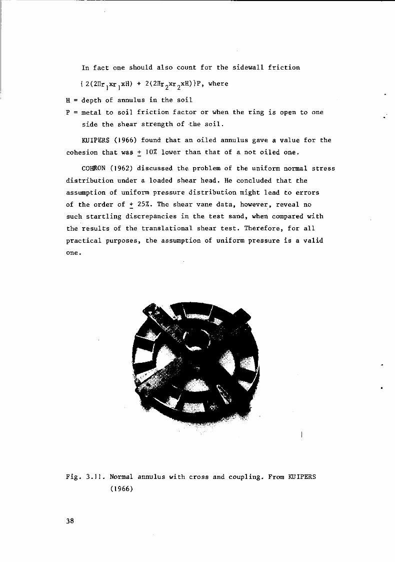
In fact one should also count for the sidewall friction
{ 2(2nrjXr]xH) + 2(2IIr2xr2xH)}P, where
H = depth of annulus in the soil
P = metal to soil friction factor or when the ring is open to one
side the shear strength of the soil.
KUIPERS (1966) found that an oiled annulus gave a value for the
cohesion that was + 10% lower than that of a not oiled one.
C0HR0N (1962) discussed the problem of the uniform normal stress
distribution under a loaded shear head. He concluded that the
assumption of uniform pressure distribution might lead to errors
of the order of + 25%. The shear vane data, however, reveal no
such startling discrepancies in the test sand, when compared with
the results of the translational shear test. Therefore, for all
practical purposes, the assumption of uniform pressure is a valid
one.
Fig. 3.11. Normal annulus with cross and coupling. From KUIPERS
(1966)
38

3.4. S o l i d s h e a r h e a d
The shearhead is a disc with grousers. On the disc one can
apply a normal load. With this instrument one can find the shear
strength under different normal load conditions and so the cohesion
and the angle of internal friction can be found (COH. ON, 1962).
The formula for the shear strength
where
P = 3M
211 R3
T = shear strength
M = torque to shear in the soil
R = diameter of disc (see fig. 3.12)
Fig. 3.12. Torsional shearhead. From BAILEY (1965)
39

LITERATURE SHEAR ANNULUS AND SOLID SHEARHEAD. Chapter 3.3. and 3.4.
AGRICULTURAL HANDBOOK no. 316 - Soil dynamics in tillage and traction.
United States department of agriculure.
BAILEY, A.C. and J.A. WEBER. Comparison of Methods of Measuring Soil
Shear Strength Using Artificial Soils - Transactions of the
ASAE - vol. 8 no. 2, p. 153.
COHNON, GERALD T. The soil sheargraph. Presentation at the 1962 annual
Meeting American society of agricultural Engineering.
KUIPERS, H and B. KROESBERGEN. The significance of moisture content,
pore space, method of sample preparation and type of shear
annulus used on laboratory torsional shear testing of soils.
Journal of Terramechanics, 1966, vol. 3, no. 4, pp. 17 to 28.
40
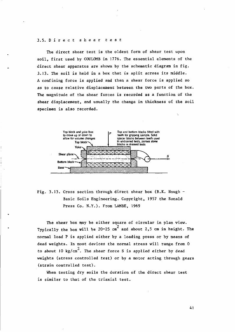
3.5. D i r e c t s h e a r t e s t
The direct shear test is the oldest form of shear test upon
soil, first used by COULOMB in 1776. The essential elements of the
direct shear apparatus are shown by the schematic diagram in fig.
3.13. The soil is held in a box that is split across its middle.
A confining force is applied and then a shear force is applied so
as to cause relative displacement between the two parts of the box.
The magnitude of the shear forces is recorded as a function of the
shear displacement, and usually the change in thickness of the soil
specimen is also recorded.
Top block and yoke free to move up or down to allow for volume changes
Top block
Yoke
Shear plane
Top and bottom blocks fitted with teeth for gripping sample. Solid spacer blocks between teeth used in undrained tests, porous stone blocks in drained tests
Fig. 3.13. Cross section through direct shear box (B.K. Hough -
Basic Soils Engineering. Copyright, 1957 the Ronald
Press Co. N.Y.). From LAMBE, 1969
The shear box may be either square of circular in plan view. 2
Typically the box will be 20-25 cm and about 2,5 cm in height. The
normal load P is applied either by a loading press or by means of
dead weights. In most devices the normal stress will range from 0 2
to about 10 kg/cm . The shear force S is applied either by dead
weights (stress controlled test) or by a motor acting through gears
(strain controlled test).
When testing dry soils the duration of the direct shear test
is similar to that of the triaxial test.
41

The shear box can also be used in the field (see fig. 3.15).
i -F
3 . "-.•; •:.' • ".'.••'. E !
Reaction
• .Sahd Fill V
Ml E
laad//>g Jack
3D * SO cm
•Sheer Box \ \ \
Surcharge
M
Fig. 3.15. Scheme used for field direct shear tests from ZEITLER,
1966
42
LITERATURE DIRECT SHEAR BOX. Chapter 3.5.
LAMBE and WHITMAN, 1969. Soil Mechanics. Massachusetts Institute of
of Technology John Wiley and Sons, Inc. New York.
ZEITLER, JOSEPH G. and Y. NEGNI, 1966. Study of horizontal and ver
tical loading tests on a sand. Technion - Israel institute
of technology. Faculty of civil engineering. Publication no.
31.
43
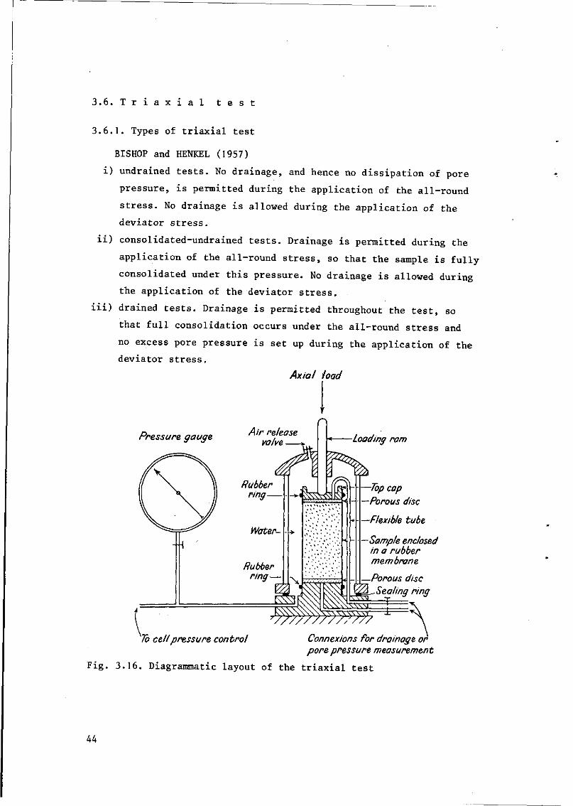
3.6. T r i a x i a l t e s t
3.6.1. Types of triaxial test
BISHOP and HENKEL (1957)
i) undrained tests. No drainage, and hence no dissipation of pore
pressure, is permitted during the application of the all-round
stress. No drainage is allowed during the application of the
deviator stress,
ii) consolidated-undrained tests. Drainage is permitted during the
application of the all-round stress, so that the sample is fully
consolidated under this pressure. No drainage is allowed during
the application of the deviator stress,
iii) drained tests. Drainage is permitted throughout the test, so
that full consolidation occurs under the all-round stress and
no excess pore pressure is set up during the application of the
deviator stress.
Axial load
Pressure, gauge Air release valve
Rubber ring-
-\ Water-
Rubber ring
Loading ram
—Top cap —Porous disc
—Flexible tube
—Sample enclosed in a rubber membrane
—Porous disc Sealing ring =$= =£=
To cell pressure control Connexions for drainage or pore pressure measurement
Fig. 3.16. Diagrammatic layout of the t r i ax i a l t e s t
44

3.6.2. Urtdrained test on saturated cohesive soils
The test is carried out on undisturbed samples of clay, silt
and peat as a measure of the strength of the natural ground; and
on remoulded samples of clay when measuring sensitivity or carrying
out model tests in the laboratory.
The deviator stress as failure is found to be indepent of the
cell pressure (with the exception of fissured clays and compact
silts at low cell pressure).
If shear strength is expressed as a function of total normal
stress by Coulomb's empirical law:
Tf = cu + atg<(>4
cu = apparent cohesion with respect to changes in
<t>4 = angle of shearing resistance total stress
Then it follows that, in this particular case
<t>4 = 0
cu = \ (ol-o3)
Total stresses
hH \-u-A
Fig. 3.17. Mohr stress circles for undrained tests on saturated
cohesive soils
45
The shear strength of the soil, expressed as the apparent co
hesion, is used in a stability analysis carried out in terms of
total stress, which, for this type of soil, is known as the $ = 0
analysis.
For saturated clays both the major principal effective stress
a = (al-u) and the minor principal effective stress a (=a3-u) are
independent of the magnitude of the cell pressure applied (u = pore
pressure). Hence only one effective stress circle is obtained from
these tests and the shape of the failure envelope in terms of effec
tive stress cannot be determined.
Because the sample as used here has another stress history than
the soil in situ no pore-pressure measurements are made during un-
drained tests on saturated samples.
The failure stress is taken to be the maximum deviation stress
which te sample can withstand.
Where the stress-strain curve has a pronounced peak this value
is unambiguous. In some soils which have softened after being heavily
consolidated, and in remoulded soils, failure takes the form of
plastic yield at a constant stress and occurs only after very large
axial strains. Termination of the test at an arbitrary strain of 10%
or even 20% may lead to an underestimate of strength.
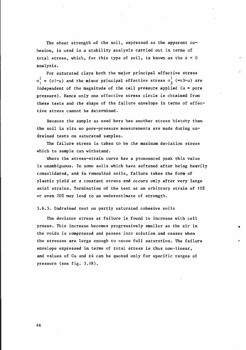
3.6.3. Undrained test on partly saturated cohesive soils
The deviator stress at failure is found to increase with cell
presse. This increase becomes progressively smaller as the air in
the voids is compressed and passes into solution and ceases when
the stresses are large enough to cause full saturation. The failure
envelope expressed in terms of total stress is thus non-linear,
and values of Cu and <(>4 can be quoted only for specific ranges of
pressure (see fig. 3.18).
46
T s ' \ ?^ Effective stresses
^ _ £ _ y-Total stresses
Fig. 3.18. Mohr stress circles for undrained tests on partly
saturated soil, (a) total stresses, (b) effective
stresses
If the pore pressure is measured during the test, as is now
more usual, the failure envelope can be expressed in terms of
effective stress (fig. (b)), and is found to approximate very
closely to a straight line over a wide range of stress.
Apparent departures from linearity are usually found to be due
to small differences in water content between the three or four
samples used to define the envelope.
3.6,4. Consolidated-undrained test on saturated soils
In the standard test the sample is allowed to consolidate under a
cell pressure of known magnitude (P), the three principal stresses
thus being equal.
Then the sample is sheared under undrained conditions by applying
47
an axial load. As in the case of the undrained test, the cell pres
sure at which the sample is sheared does not influence the strength
(except of dilatant sands).
The test result, in terms of total stresses, may thus be ex
pressed as the value of cu, the apparent cohesion, plotted against
consolidation pressure P. For normally consolidated samples the
ratio cu/P is found to be a constant, its value depending on the
soil type. However, undrained triaxial tests and vane tests on
strata existing in nature in a normally consolidated state lead to
a lower estimate of the ratio cu/P than is found in samples con
solidated under equal all-round pressure in laboratory. The diffe
rence increases as the plasticity index decreases and may be attri
buted mainly to two causes.
1) A naturally deposited sediment is consolidated under conditions
of no lateral displacement and hence with a lateral effective
stress considerably less than the vertical stress. The ratio of
lateral effective stress to the vertical effective stress, termed
the coefficient of earth pressure at rest, generally lies in the
range 0.7-0,35, the lower values occurring in soils with a low
plasticity index. The reduction in the value of cu/P which results
when samples are consolidated in the laboratory under this stress
ratio, instead of under equal all-round pressure, may be as much
as 50%.
2) Reconsolidation in the laboratory after the disturbance which is
associated even with the most careful sampling leads to a slightly
lower void ratio than would occur in nature. The value of the pore-
pressure parameter A in particular is sensitive to the resulting
modification in soil structure an this, in turn, leads to a higher
undrained strength - (Au=B(Aa3+A(A.al-Aa3) ) -.
For these reasons the results of consolidated-undrained tests,
expressed in terms of total stress, can be applied in practice only
to a very limited extent. If the pore pressure is measured during the
undrained stage of the test, the results can however be expressed
in terms of effective stress. The values of c and <)> thus obtained
can be applied to a wider range of practical problems.
48

(o)
I
(O + /0
OS
Af
Consolidation pressure p
Consolidation pressure p i i
\b
-OS
Consolidation pressure p
(d) T
c'^ •if^a
J t - " " ^
c «^ ^Tf
» Effective normal stress <r'
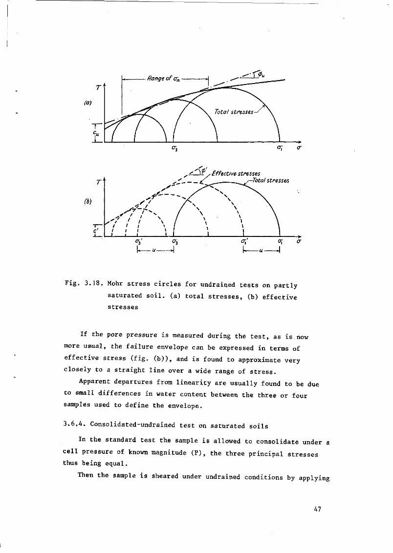
Fig. 3,19. Consolidated-undrained tests on saturated soil
(a) water content,
(b) undrained strength, and
(c) value of A , plotted against consolidation pressuere p;
(d) Mohr envelope in terms of effective stress.
49

In fig. 3.19 the relationships between the total stress, pore
pressure and effective stress characteristics are illustrated. The
points a, b and c represent normally consolidated samples; the point
d represents an over-consolidated sample, the over-consolidation
ratio being Pb/Pd (fig. 3.19(a)). For normally consolidated samples
the effective stress envelope (fig. 3.19(d)) is a straight line with
c equal to zero, <(> depending on the type of soil. Over-consolidation
results in an envelope lying a little above this straight line; a
section of this envelope, over a specified stress range, being re
presented with sufficient accuracy by a slightly modified value of <j>
and a cohesion intercept c .
The most marked effect of over-consolidation is, however, on
the value of A, which, with increasing over-consolidation ratio,
drops from a value typically about 1 at failure to values in the
negative range.
These low A-values are, in turn, largely responsible for the
high undrained strength values resulting from over-consolidation
(compare point d, fig. 3.19(b), with point a ) . Values of c and $
are usually based on the effective stress circles corresponding
to maximum deviator stress. In tests on over-consolidated clay
samples and on samples of sand the limited values of c and $ may
occur at an intermediate stage, as explained in the previous section.
Here again the difference is of importance only in research inves
tigations, a typical result for sands being an underestimate of (|>
by about 2 .
3.6.5. Consolidâted-undrained test on partly saturated soils
This test may be called for in the determination of c and <|>
on undisturbed samples or on compacted samples of earth fill, in
particular when the degree of saturation is not low enough to result
in a sufficient range of strenghts in the undrained test to define
a satisfactory failure envelope. It may also be used to examine the
effect of c and $ of flooding foundation strata and earth-fill
materials, and indicates the magnitude of the accompanying volume
change.
Flooding, even for a period of months under an appreciable
50
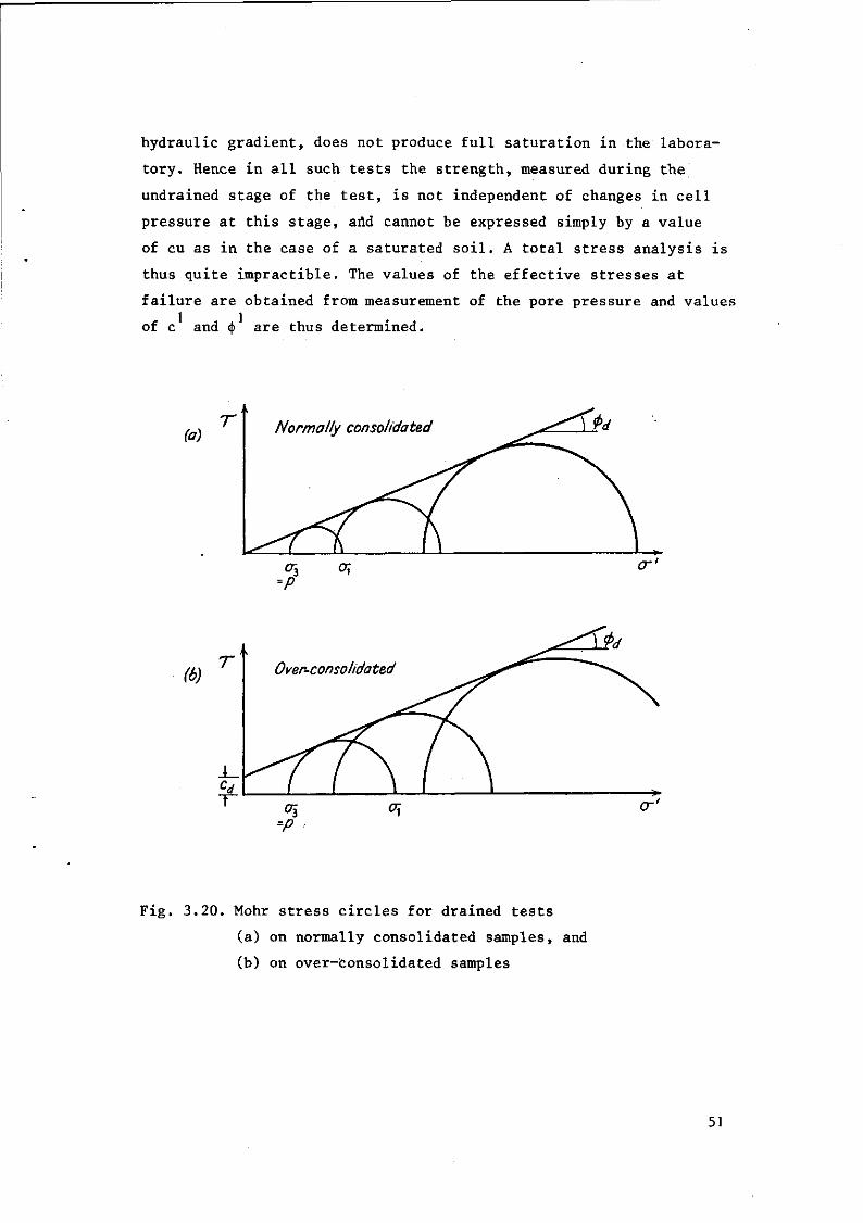
hydraulic gradient, does not produce full saturation in the labora
tory. Hence in all such tests the strength, measured during the
undrained stage of the test, is not independent of changes in cell
pressure at this stage, and cannot be expressed simply by a value
of cu as in the case of a saturated soil. A total stress analysis is
thus quite impractible. The values of the effective stresses at
failure are obtained from measurement of the pore pressure and values
of c and <j> are thus determined.
(a) T Normally consolidated
(b)
=P
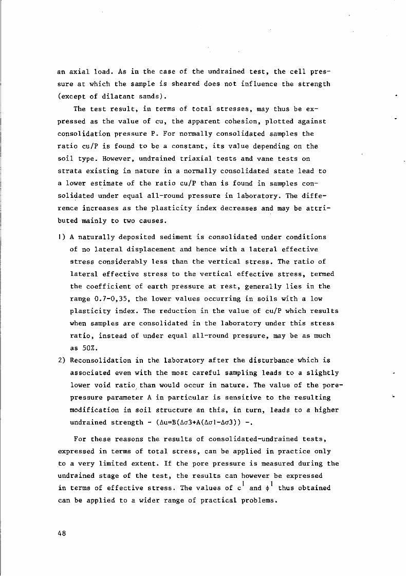
Fig. 3.20. Mohr stress circles for drained tests
(a) on normally consolidated samples, and
(b) on over-consolidated samples
51

3.6.6. Drained tests
Drained tests are carried out on soil samples of all types either
undisturbed, remoulded, compacted or redeposited. The samples may be
either fully or partly saturated. Cohesionless materials such as
sand, gravel and rock-fill are often tested dry as it simplifies
laboratory procedure. This may, however, lead to a slight over
estimate of the value of $ in some cases. Tests on sugar, grain,
etc., for silo design are also performed under normal "air-dried"
conditions.
In the standard test consolidation takes place under an equal
all-round pressure, and the sample is then sheared by increasing
the axial load at a sufficiently slow rate to prevent any build-up
of excess pore pressure. The minor principal stress a at failure
is thus equal to p, the consolidation pressure; the major principal
stress a. is the axial stress. Since the pore pressure is zero, the
effective stresses are equal to the applied stresses, and the strength
envelope in terms of effective stress is obtained directly from the
stress circles at failure, fig. 3.20. The values of c and $ obtained
from drained tests are often denoted cd and <j)d respectively. The
drained test also provides information on the volume changes which
accompany the application of the all-round pressure and the deviator
stress, and on the stress-strain characteristics of the soil.
3.6.7. General remarks on the interrelationship of the test results
1) For a given sample of soil the shear strength parameters c arid <j>
are almost independent of the type of test used to measure them
with the following qualifications:
a) For normally consolidated clays the values of c and <j> ob
tained from consolidated-undrained tests with pore-pressure
measurement and from drained tests are, for practical purposes,
identical provided comparable rates of testing are used.
b) For heavily over-consolidated clays and for sands (except in
a very loose state) the drained test will lead to slightly
higher values of c and $ , due to the work done by the in
crease in volume of the sample during shear and to the smaller
strain at failure.
52

c) For some compacted fiixb aud other partly saturated samples
the value of c will be reduced if an increase in water content
occurs in the consolidated-undrained or drained test.
2) In contrast, deformation and volume-change characteristics in
drained tests, and pore-pressure and undrained strength charac
teristics in consolidated-undrained tests, are largely controlled
by the sequence and sign of the stress changes.
For practical purposes one should always simulate the stresses
that occur in the soil under investigation and one has to decide
whether the soil has to be studied under drained or undrained con
ditions.
3.7. U n c o n f i n e d c o m p r e s s i o n t e s t
The unconfined compression test is in a sense a special form of
triaxial test in which there is no horizontal pressure so the minor
and intermediate principal stresses are zero. It is widely used in
practice both in the field and for routine laboratory soil testing.
It is used only on cohesive soils as such material does not require
lateral support.
The in the test most commonly employed cylindrical sample is
confined between end plates and loaded to failure by increase in
axial pressure. Load has been applied by various means such as
spring and hydraulic systems.
As in the triaxial test and unlike the direct shear test the
failure surface is not pre-determined.
Failure may therefore occur in the weakest portion of the clay
cylinder. The mid-portion of the sample is, however, subject to the
greatest strain as the end portions are restrained laterally by the
end plates.
If the sample fails in a brittle manner a definite maximum load
before failure is recorded.
When plastic failure takes place no maximum load is reached and
the strength at some arbitrarily defined strain such as 20% is taken
in place of the peak.
53

LITERATURE TRIAXIAL TEST. Chapter 3.7.
BISHOP, ALAN W. and D.J. HENKEL, 1962. The measurements of soil
properties in the triaxial test. Edward Arnold (publishers)
L.T.D., London.
54

3.8. T h e d i f f e r e n t t e s t p r o c e d u r e s a n d
t h e i r c o r r e l a t i o n s
3.8.1. Correlations, of cone resistance and vane shear strength for
clays
LUNNE (1976) found a relationship between the cone factor N, and
the vane shear strength measured in Scandinavian soft to medium stiff
clays.
Terzaghi suggested the following formula
qc = N, af + Y-z.
where qc = cone resistance
N, = cone factor k
rf = undrained shear strength
Y = total unit wheight of soil
z = depth of penetration
After the application of the correction factor of Bjerrum for
Scandinavian clays (see LUNNE, 1976) Lunne found a value of 15 to 19
for the N, factor for soft to medium stiff clay with different
plasticity (see fig. 3.21).
70
2
ce o •—
< 1S LL
O O 2 io i— u LU CC ce o o
/
RANGE IN SENSITIVITY
>Sfl
15-ïS V
Î OG 1-4
10-tS O
A S-10
Î-9 a +
13-1?
LEGENDJ O SUWOL AND
D DANVIKSG1
V £ B0ff«ESENS &T
A ONS0Y
+ G0TEBOR3
x SKÂ-EDEBV I I L- -
36
X 10-15
15-24
+
IÎ-I9
X 6-10
Plasticity = water content of
soil between the
plastic limit and
liquid limt.
10 20 60 SO 60
P L A S T I C I T Y , l p , %
Fig. 3.21. Summary of corrected N values from all sites
55
3.8.2. Correlations of vane-test, unconfined compression test and
undrained-unconsolidated triaxial test
Vane shear tests and shear annulus tests are used to determine
the undrained shear strength of saturated or nearly saturated co
hesive soils.
In principle one should find the same values for the shear
strength as with the undrained-unconsolidated triaxial compression
test.
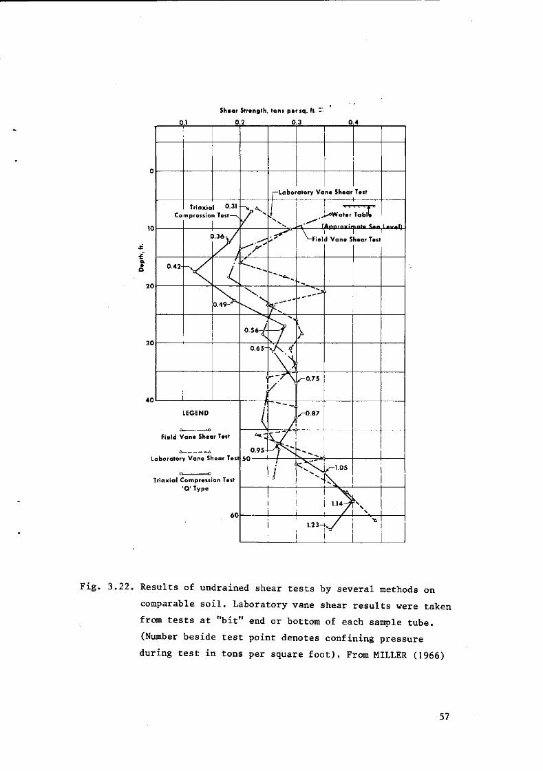
MILLER (1966) found that the shear strength as obtained by tri
axial methods was lower than by field and laboratory vane methods
for samples tested to a depth of about 7,5 m, with close agreement
below this depth (see fig. 3.22).
HALL (1963) reported that strengths determined by field vane
tests were consistently higher than laboratory compression tests
throughout the entire depth.
SIBLEY (1966) found that the correlation between the hand-
operated torsional vane shear test results and those from uncon
fined and triaxial tests oil saturated clays having shear strengths 2
below 1 kg/cm was very good (fig. 3.23).
SUDHINDRA and MELKOTE (1974) found for sensitive clays (sen
sitivity 5) that the unconfined compression test gave significantly
lower values as compared with either the deviator stress at failure
in an unconsolidated undrained triaxial test or the field vane shear
test results.
However the unconfined compression test was done in the field
immediately after sampling, whereas the triaxial shear tests were
done a few weeks later at the laboratory. The samples gain in strength
after sampling.
VENEMAN (1976) found with the vane shear test somewhat higher
values than with the unconfined compression test.
The sensitivity of the clay is the ratio of the shear strength of an undisturbed sample to the remoulded strength. Clays have been subdivided into classes on the basis of their sensitivity as shown in table 3.2.
56
Shear Strength, tons per sq. ft. -•
0.1 0.2 0.3 0.4
Triaxial Compression Test 'Q' Type
Fig. 3.22. Results of undrained shear tests by several methods on
comparable soil. Laboratory vane shear results were taken
from tests at "bit" end or bottom of each sample tube.
(Number beside test point denotes confining pressure
during test in tons per square foot). From MILLER (1966)
57

lÛO
Z 0.80
0.60
0.40
a. < 0.20
A
> W •9
y
~7\
/ X^/~t
4 A/
£* *£
/
0 0.20 0.40 0.60 0.80 1.00
VANE SHEAR STRENGTH SV| in tons/sq.ft.
* i
LEGEND
A SucSLOW - Unconfined compression test, slow test : Suc = 1/2 qu -J
* SUCFAST - Unconfined compression test, quiektest- Suc = 1/2 qu •
• SQ - Triaxial compression test, Q test: S0 = 1/2 (»j-a^lmax.
qu Unconfined compressive strength
Fig. 3.23. Torsional vane shear strength relationship with other
strength tests, Bootlegger Cove clay. From SIBLEY (1966)
.. 1 Tabel 3.2. Classification of clay sensitivity (after LEONARDS, 1962,
p. 78)
Sensitivity Classification
< 2
2-4
4-8
8-16
16-32
32-64
>64
Insensitive
Moderately sensitive
Sensitive
Very sensitive
Slightly quick
Medium quick
Quick
Reproduced by permission of McGraw-Hill Book Company, Inc., New York, N.Y. From GILLOT, 1968
58

3.8.3. Correlations of cone index, triaxial test and vane test
W.E.S. (1964) stated the following relationship between the
different measuring devices.
cone index = triaxial cohesion x 12,5 = vane shear strength x 10
for soils with a low shear strength and in which the friction angle
is small 4 < 4
and
triaxial max. shear strength = vane shear strength + 0.6 psi
(see fig. 3.24 and 3.25).
The bevameter results given by the W.E.S. are too confusing and
because this method is seldom used this measuring devise is'not
mentioned in this review.
LAMBE and WHITMAN (1969) give the following accuracy for the
different test methods (tabel 3.3).
Table 3.3. Common Methods for Measuring Undrained Strength.
From LAMBE (1969)
Method Comment
In-situ measurements
1. Vane test Usually considered to give best result, but is limited as to strength of soil with which it can be used
2. Penetration test Gives crude correlation to strength
Measurements upon undisturbed samples
1. Unconfined compression Best general purpose test; underestimates strength because disturbance decreases effective stress
2. UU test at in situ con- Most representative of laboratory fining pressure tests, because of compensating errors
3. CU test at in situ con- Overestimates strength, because dis-fining pressure turbance leads to smaller water con
tent upon reconsolidation
UU = unconfined undrained triaxial test
CU = confined undrained triaxial test.
59
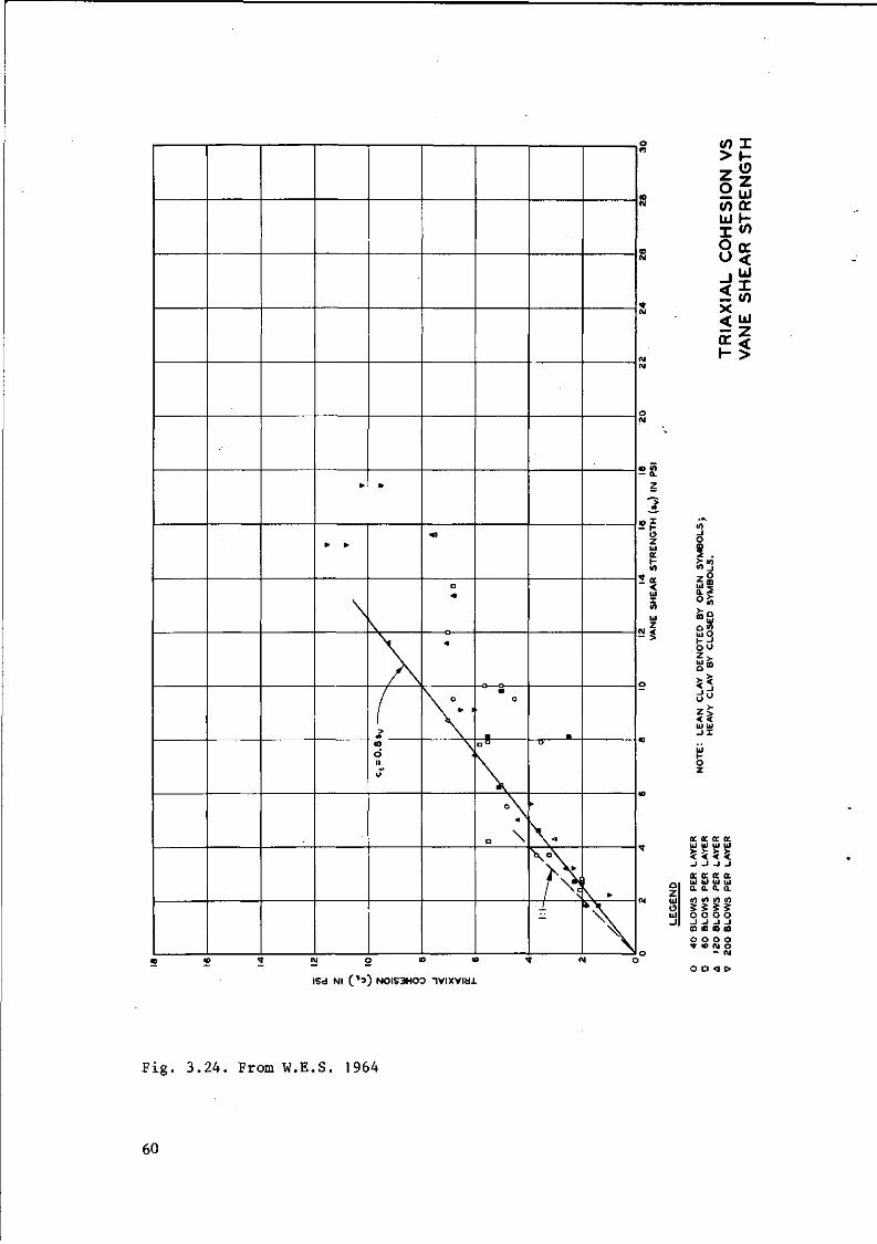
-0-8-
0> > Z O (f) UI I O u
X < cc I -
X h-e> z UI tr y-tn
cc < ui I </>
UI
z 2
'f o z UJ ir i-<o
z
«2
« - I o o 2 . is*) 7 0
(0
' Ui
w o «o «o
ISd NI ( * s ) NOIS3HO0 HVIXViai
û •> UI O
z ,
SI UI UI J I
ui I-o z
(T CC CC CC UI UI UJ UI
-J J -J _J
cc er o: er ui UI UJ UI
a. a o. a. •o m 10 « Ï S J Î o o o o J J J J CO CO 03 ID o o o o 9 D M O
- 01
F ig . 3 .24 . From W.E.S. 1964
60

24
22
20
18
o.
•n 16
A
c
0
n'A / " o
ji
o . A y^
A
0
A
•
(
• /
/ 8
»
• V
>
1 /
/ à
>v = »MAX +
D
' /*
0.6 ^
»
T
»
8 10 12 VANE SHEAR STRENGTH (sv) IN PSI
20
LEGEND
O 4 0 BLOWS PER LAYER 0 6 0 BLOWS PER LAYER b. 120 BLOWS PER LAYER V 2 0 0 BLOWS PER LAYER
NOTE: LEAN CLAY DENOTED BY OPEN SYMBOLS; HEAVY CLAY BY CLOSED SYMBOLS.
MAXIMUM TRIAXIAL SHEAR STRENGTH VS VANE
SHEAR STRENGTH
Fig . 3 . 25 . From W.E.S. (1964)
61
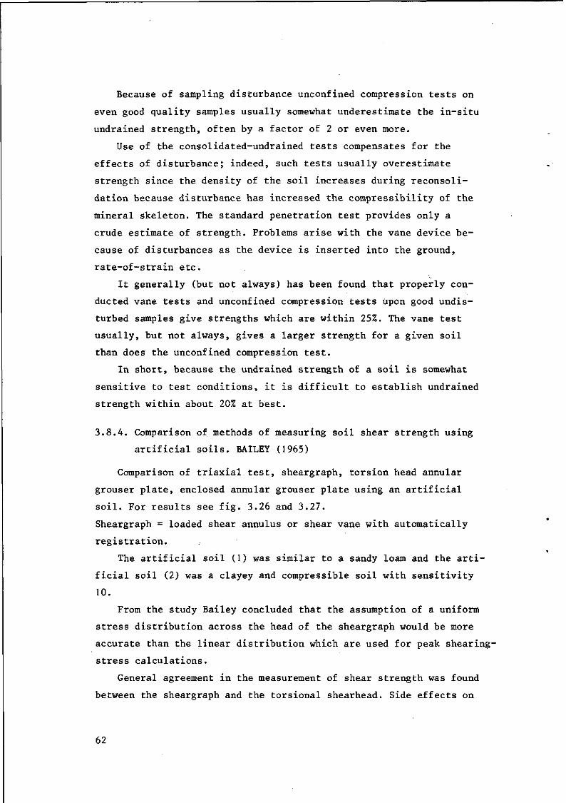
Because of sampling disturbance unconfined compression tests on
even good quality samples usually somewhat underestimate the in-situ
undrained strength, often by a factor of 2 or even more.
Use of the consolidated-undrained tests compensates for the
effects of disturbance; indeed, such tests usually overestimate
strength since the density of the soil increases during reconsoli
dation because disturbance has increased the compressibility of the
mineral skeleton. The standard penetration test provides only a
crude estimate of strength. Problems arise with the vane device be
cause of disturbances as the device is inserted into the ground,
rate-of-strain etc.
It generally (but not always) has been found that properly con
ducted vane tests and unconfined compression tests Upon good undis
turbed samples give strengths which are within 25%. The vane test
usually, but not always, gives a larger strength for a given soil
than does the unconfined compression test.
In short, because the undrained strength of a soil is somewhat
sensitive to test conditions, it is difficult to establish undrained
strength within about 20% at best.
3.8.4. Comparison of methods of measuring soil shear strength using
artificial soils. BAILEY (1965)
Comparison of triaxial test, sheargraph, torsion head annular
grouser plate, enclosed annular grouser plate using an artificial
soil. For results see fig. 3.26 and 3.27.
Sheargraph = loaded shear annulus or shear vane with automatically
registration.
The artificial soil (1) was similar to a sandy loam and the arti
ficial soil (2) was a clayey and compressible soil with sensitivity
10.
From the study Bailey concluded that the assumption of a uniform
stress distribution across the head of the sheargraph would be more
accurate than the linear distribution which are used for peak shearing-
stress calculations.
General agreement in the measurement of shear strength was found
between the sheargraph and the torsional shearhead. Side effects on
62
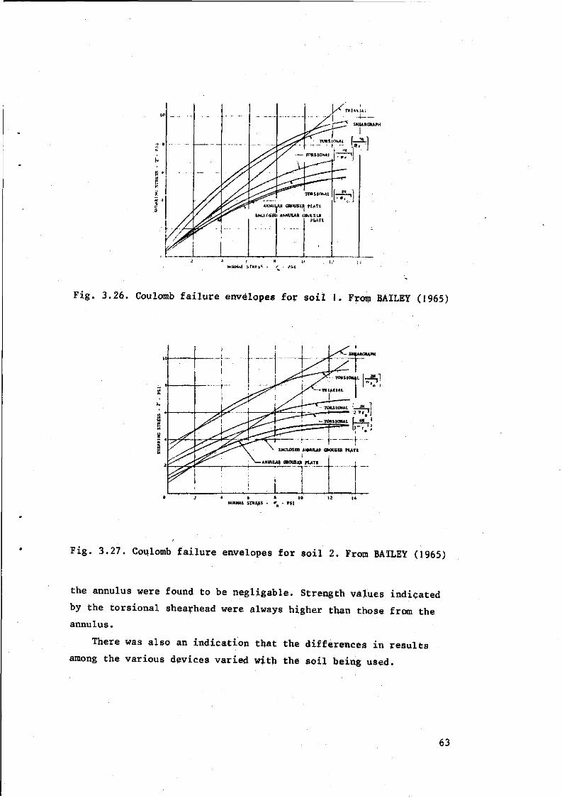
SHEARCRAfH
\/^ T» l* \ lAi
WtUM̂ if iTHtiS . ) . ,»*,(
Fig. 3.26. Coulpmb failure envelopes for soil 1. From BAILEY (1965)
W*MM ST«t*S . r - PS I
Fig. 3.27. Coylomb failure envelopes for soil 2, From BAILEY (1965)
the annulus were found to be negligable. Strength values indicated
by the torsional shearhead were always higher than those from the
annulus.
There was also an indication that the differences in results
among the various devices varied with the soil being used.
63

-o -o
• - i oo « e
C " 3 <a
U J2
a E
c
c 3
1
1
<S
3
>
O
1
1 E
.1
1
C
3 | - oo • «
• T3 l d 0
3 oo
C e
g - o " «
3 O • O
i c
O.
I
i e
ex
1 •o
3
.£5
•c E w E V
M 0 Q U E O « OS - < •
e
e E - •
e «
• « os c c — c
i n W M D . «
» •§ d « f d ? i â ï ë g S S
H 0
c
>
3
1 e
— w
1 c
0
«
ib s
e o-, ra
S e "E
H M C - J -c =c o CQ Û o o - o = e
3 3
a
e
•O E O c o m 3 in u*
1
c o c
c -2 3 ra
64
LITERATURE CHAPTER 3.8.
BAILEY, A.C. and J.A. WEBER, 1965. Comparison of Methods of Measu
ring soil shear strength using artificial soils. Transactions
of the ASAE vol. 8, no. 2, p. 153.
GILLOT, J.E., 1968. Clay in engineering geology. Elsevier Publishing
Company, Amsterdam.
LAMBE, T. WILLIAM and ROBERT V. WHITMAN, 1969. Soil Mechanics.
Massachusetts Institute of Technology John Wiley and Sons,
Inc. New York, London, Sydney.
LUNNE, T., 0. EIDE and J. DE RUITER, 1976. Correlations between cone
resistance and vane shear strength in some Scandinavian soft
to medium stiff clays. Can. Geotech. J. 13, 430.
MILLER, E.A. and E.B. HALL, 1966. A comparison of soil shear strenghts
as determined with field and laboratory vane shear apparatus.
Vane shear and cone penetration resistance testing of in-
situ soils, ASTM STP 399, Am. Soc. Testing Mats. p. 18.
SIBLEY, E.A. and G. YAMANE, 1966. A simple shear test for saturated
cohesive soils. Vane shear and cone penetration resistance
testing of in-situ soils. ASTM STP 399, Am. Soc. Testing
Mats. p. 39.
SUDHINDRA, C. and R.S. MELKOTE, 1974. Some experiences in evaluation
of undrained shear strength of saturated sensitive clays.
Irrigation and power, vol. 31, no. 4, October.
VENEMAN, P.L.M., J. BOUWMA and T.B. EDIL, 1976. Soil shear strength
variation in soils of a Batavia Silt loam mapping unit.
Soil Sei. Soc. Am. J. vol. 40, pp. 462-465.
W.E.S., 1964. Strength-moisture-density relations of fine-grained
soils in vehicle mobility research, Technical report no. 3-
639 January. U.S. Army Engineer Waterways Experiment Station
Corps of Engineers. Vicksburg, Mississippi.
65

4. FRICTION ANGLE AND SHEAR STRENGTH OF COHESIONLESS SOILS
4 . 1 . D e f i n i t i o n o f f r i c t i o n a n g l e
Two alternative ways of expressing frictional resistance are in
common use. The first is to use the coefficient of friction <j). Thus,
if N is the normal force across a surface the maximum shear force
on this surface is Tmax = Nf.
The second is to use a friction angle <f>u defined such that
tan <)>u = f. <j)u is particle to particle friction, whereas <(> is the
analytical friction angle of the Coulomb-Mohr equation.
The geometric interpretation of 4>u is shown in fig. 4.1.
N
mm AVA\VAWAWAVA\WAV/AVA\VA\
Tm» = Nf
Fig. 4.1. Definition of friction angle <f>u. From LAMBE, 1969
4.2. F r i c t i o n b e t w e e n m i n e r a l s i n g r a
n u l a r f o r m
The particles of coarse silt have a minimum diameter of 0,002 cm
(20 u or 2000 0000 A°). The diameters of these and larger particles
are clearly larger than the height of the asperities (about 1000 -
10 000 A ) that may be expected on the surfaces of these particles.
Consequently we would expect that each apparent point of contact
between particles actually involves many minute contacts.
The surfaces of these soil particles are of course contaminated
with water molecules and various ions and possibly other materials.
These contaminants are largely squeezed out from between the actual
points of contact, although some small quantity of contaminants
66

remains to influence the shear strength of the junctions.
The minimum diameter of fine silt particles is 2 y or 20 000 A .
Such small particles have dimensions of the same order as the height
of the asperities on larger particles. For these small particles it
makes more sense to talk about "corners" rather than asperities.
Although the general nature of the frictional resistance is the same
for either large or small granular particles, an apparent contact
between very small granular particles may, in fact, consist of only
one actual contact point.
The testing systems shown in fig. 4.2. have been used to determine
the frictional resistance for minerals. When fixed buttons on sliding
blocks are used (fig. 4.2.) the results give the static (and perhaps
kinetic) coefficient of friction. When many sand particles are pulled
over a flat surface (fig. 4.2.) the results generally reflect some
combination of sliding and rolling friction. Hence the friction factor
as measured by the second type of test involving many particles may
be different from the value measured by the first type of test.
Weight •
Mineral_ block
X Mineral buttons / " o r block
J L^. , w
V; ,^: ;V, ,^ ,L^, /V, ,^ , :V, , ; . - ) *W
Reservoir
w 'Plaster of Paris
(a)
N
(b)
Fig. 4.2. Devices for measuring friction factor of mineral surfaces,
(a) Sliding on buttons or on block, (b) Sliding of many
particles
67

4 . 3 . E f f e c t o f s u r f a c e w a t e r a n d s u r f a c e
r o u g h n e s s
F i g . 4 . 3 . summarizes the f r i c t i o n f a c t o r s observed for quar tz
under va ry ing cond i t ions of sur face c l e a r l i n e s s , humidi ty , and
sur face roughness.
1.2
1.0
o 0.6
:0.4
0.2
" ~ l I I l r O • Chemical cleaning O • Normal cleaning A * No cleaning
O D A Air-dry
• • * Submerged I ) Range of values
I — I — i Very rough" i 1 1 i—
L--"[.U J..LL After Bromwell (1966) and Dickey (1966) — I — 1 — ! - • - ; - + — f — ! - - 1 — i -
I I
I
10 20 30 40 50 60 70 Average roughness (10 in.)
Fig. 4.3. Friction of quartz (after BROMWELL (1966) and DICKEY (1966)
From LAMBE (1969)
The results show that the friction of smooth quartz varies from
about f = 0.2 to f = 1.0 depending on the surface cleanliness.
For the more contaminated surfaces water increases the friction;
i.e. it acts as an antilubricant. However, for carefully cleaned
surfaces, water has no effect.
But if there is a contaminating layer (probably a thin film of
organic material) the water disrupts this layer, reduces its effec
tiveness as a lubricant, and thereby increases the friction. As the
surfaces get rougher the effects of cleaning procedure on friction
decrease, so that a very rough surface of 60 u in. (about 15 000 A )
gives essentially the same value of f independent of surface clean
liness. This indicates that the ability of the contaminating layer
68

to lubricate the surfaces decreases as the surface roughness in
creases. This is what we would expect from a thin lubricating layer
which acts as a boundary lubricant.
The fact that the rougher surfaces do not give higher values of
friction when they are carefully cleaned is more difficult to explain.
The evidence seems to indicate that the rougher surfaces cannot
be cleaned as effectively as smooth surfaces, although the reason for
this is not clear.
From a practical point of view the essentially constant value
of f = 0.5 (<t>u = 26 ) for very rough quartz surfaces is of great
significance, since essentially all quartz particles in natural soils
have rough surfaces.
Values of friction for other nonsheet minerals are summarize-
in table 4.1.
Table 4.1. Friction of Nonsheet Minerals. From LAMBE, 1969
Conditions of Surface Moisture
Mineral
Quartz
Feldspar
Calcite
Oven-Dried
0.13
0.12
0.14
Air Oven-Dried ; -Equilibrated
0.13
0.12
0.14
Saturât
0.45
0.77
0.68
21,2
37,6C
34,2e
The low values of f for these minerals in the air-day condition
probably have no practical significance, since they represent in
effective cleaning of smooth, polished surfaces. Much more data are
needed for these other minerals before one can confidently choose f
values.
FEBENE and DE BOODT (1970) gave the values for the internal
friction angle of Bredene sand with varying moisture content (fig.
4.4.).
There was little influence of the moisture content on the
friction angle.
69
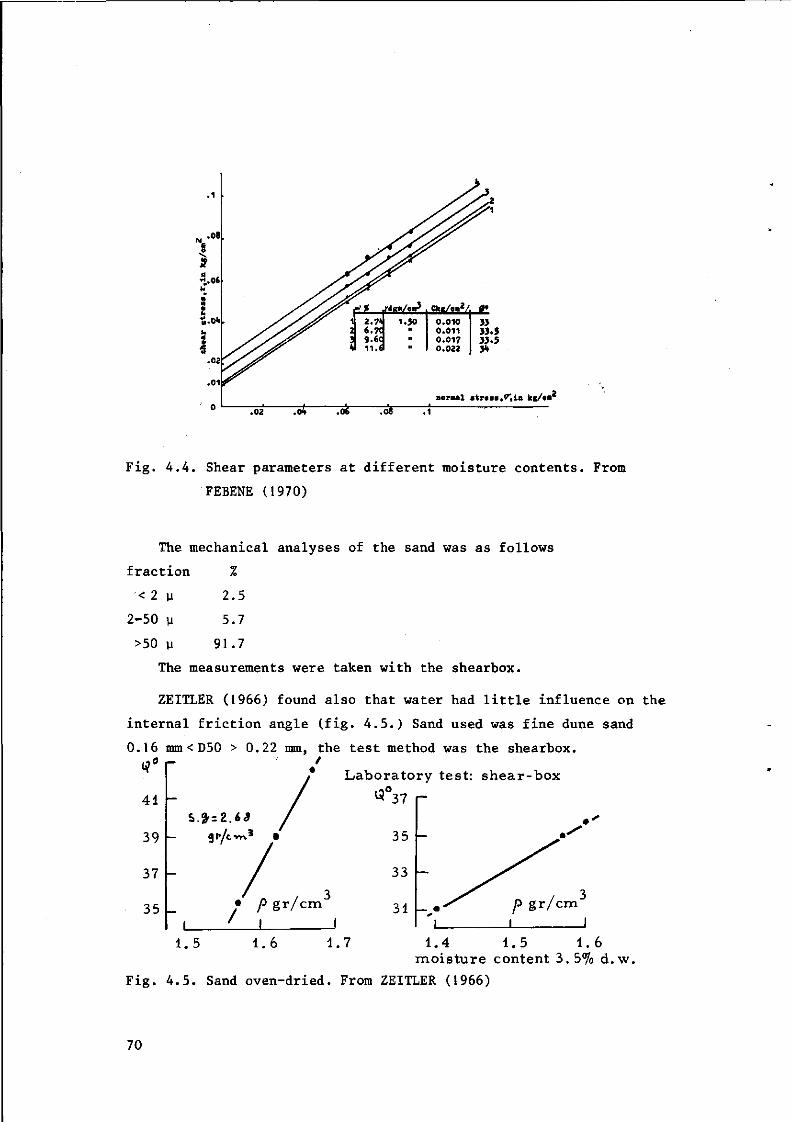
Fig. 4.4. Shear parameters at different moisture contents. From
FEBENE (1970)
The mechanical analyses of the sand was as follows
fraction %
< 2 y 2.5
2-50 y 5.7
>50 y 91.7
The measurements were taken with the shearbox.
ZEITLER (1966) found also that water had little influence on the
internal friction angle (fig. 4.5.) Sand used was fine dune sand
0.16 mm<D50 > 0.22 mm, the test method was the shearbox.
Laboratory test: shear-box
1.5 1.6 1.7
Fig. 4.5. Sand oven-dried. From ZEITLER (1966)
1.4 1.5 1.6 moisture content 3. 5% d.w.
70
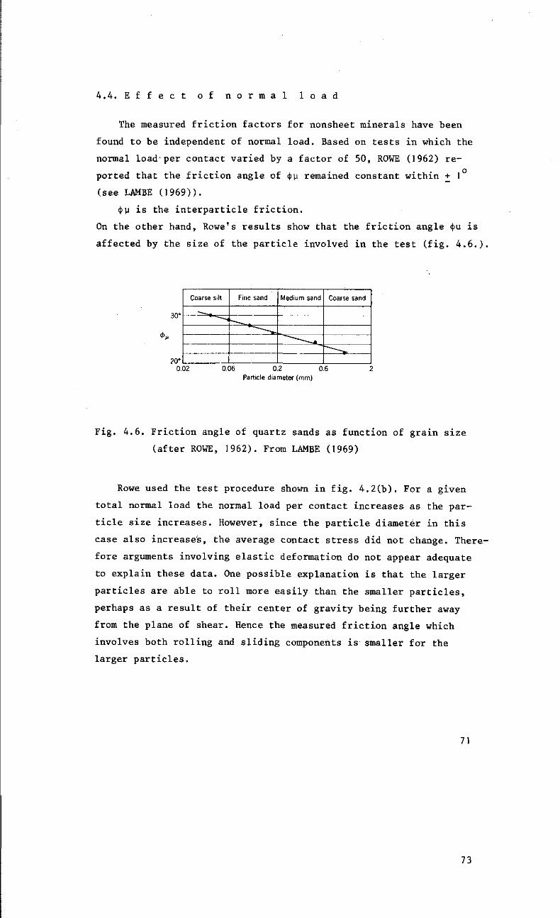
4.4. E f f e c t o f n o r m a l l o a d
The measured friction factors for nonsheet minerals have been
found to be independent of normal load. Based on tests in which the
normal load-per contact varied by a factor of 50, ROWE (1962) re
ported that the friction angle of <j>u remained constant within + 1
(see LAMBE (1969)).
<(>u is the interparticle friction.
On the other hand, Rowe's results show that the friction angle <j>u is
affected by the size of the particle involved in the test (fig. 4.6.)
30'
* M
20"
Coarse silt
-^^
Fine sand Medium sand
~"~--~-^.
Coarse sand
0.02 0.06 0.2 0.6 Particle diameter (mm)
Fig. 4.6. Friction angle of quartz sands as function of grain size
(after ROWE, 1962). From LAMBE (1969)
Rowe used the test procedure shown in fig. 4.2(b). For a given
total normal load the normal load per contact increases as the par
ticle size increases. However, since the particle diameter in this
case also increases, the average contact stress did not change. There
fore arguments involving elastic deformation do not appear adequate
to explain these data. One possible explanation is that the larger
particles are able to roll more easily than the smaller particles,
perhaps as a result of their center of gravity being further away
from the plane of shear. Hence the measured friction angle which
involves both rolling and sliding components is smaller for the
larger particles.
71
73
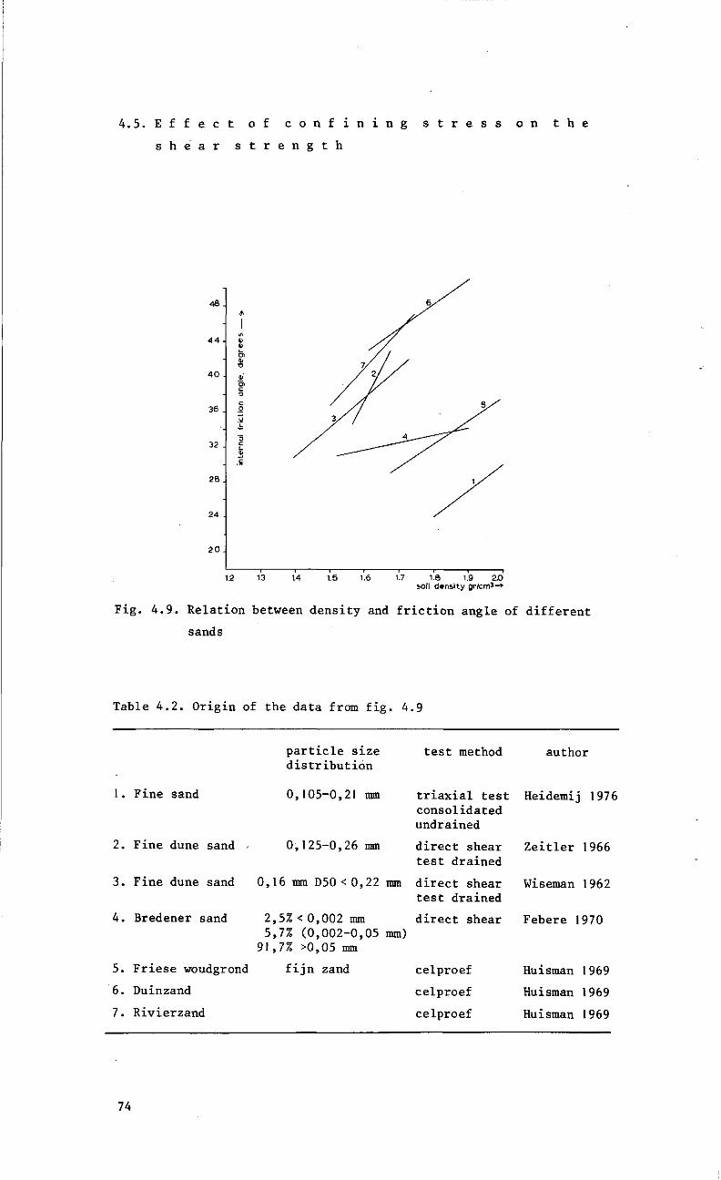
4.5. E f f e c t o f c o n f i n i n g s t r e s s o n t h e
s h e a r s t r e n g t h
48
44
40
36
32 .
28
24
2 0 .
1.2 1.3 1.4 1.5 1.6 1.7 1.8 1.9 2.0 soil density gr/cm3—»
Fig. 4.9. Relation between density and friction angle of different
sands
Table 4.2. Origin of the data from fig. 4.9
1. Fine sand
2. Fine dune sand
3. Fine dune sand
4. Bredener sand
5. Friese woudgrond
6. Duinzand
7. Rivierzand
particle size distribution
0,105-0,21 mm
0,125-0,26 mm
test method
triaxial test consolidated undrained
direct shear test drained
0,16 mm D50<0,22 mm d i r e c t shear test drained
2,5%<0,002 mm direct shear 5,7% (0,002-0,05 mm)
91,7% >0,05 mm
fijn zand celproef
celproef
celproef
author
Heidemij 1976
Zeitler 1966
Wiseman 1962
Febere 1970
Huisman 1969
Huisman 1969
Huisman 1969
74
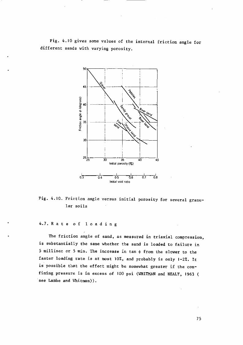
Fig. 4.10 gives some values of the internal friction angle for
different sands with varying porosity.
25 30 35 40 Initial porosity (%)
45
0.3 0.4 0.5 0.6 0.7 0.8 Initial void ratio
Fig. 4.10. Friction angle versus initial porosity for several granu
lar soils
4.7. R a t o f l o a d i n g
The friction angle of sand, as measured in triaxial compression,
is substantially the same whether the sand is loaded to failure in
5 millisec or 5 min. The increase in tan <}> from the slower to the
faster loading rate is at most 10%, and probably is only 1-2%. It
is possible that the effect might be somewhat greater if the con
fining pressure is in excess of 100 psi (WHITMAN and HEALY, 1963 (
see Lambe and Whitman)).
75

4.8. V i b r a t i o n s a n d r e p e a t e d l o a d i n g s
Repeated loadings, whether changing slowly or quickly, can cause
<(> to change. A loose sand will densify, with resulting strength in
crease, and a dense sand can expand, with resulting strength decrease.
A stress smaller than the static failure stress can cause very
large strains if the load is applied repeatedly (SEED and CHAN, 1961),
see LAMBE, 1969.
4.9. A v e r a g e p a r t i c l e s i z e
Fig. 4.11 shows data for five soils all having a uniformity
coefficient of 3.3 but having different average particle sizes. For
a given compactive effort, these sands achieve different void ratios,
e , however, the friction angle was much the same for each sand.
The effect of the greater initial interlocking in the sand with the
largest particles is compensated by the greater degree of grain
crushing and fracturing that occurs with the larger particles be
cause of the greater force per contact.
Crushing of particles and the consequent curvature of the Mohr
envelope is most important with large particles, especially gravel-
sized particles or rock fragments used for rockfills. This is be
cause increasing the particle size increases the load per particle,
and hence crushing begins at a smaller confining stress.
4.10. D e t e r m i n a t i o n o f i n - s i t u f r i c t i o n
a n g l e
The results presented in the foregoing sections have emphasized
the predominant role of the degree of interlocking upon magnitude
of the friction angle. Thus, if we wish to determine the friction
angle of a sand in-situ, it is not enough to find the nature and
shape of the particles composing the sand. It is essential to know
how tightly together these particles are packed in their natural
state. It is extremely difficult to obtain samples of a sand without
changing the porosity. Thus, except for problems involving man-made
fills, it is difficult to either measure or estimate the friction
76

Maximum particle size (mm) 0.55 i / 1 0.65
0.50
eo
0.45
0.40
0.35
/ Curve connecting ^. /points of comparable
^ v r compactive effort
v
38
\
'12
^ r \ 4 if
-50
40 42 <£ (degrees)
(a)
0.60
c 0
0.55
0.50
0.45 L_ 44 36
Average particle size (mm)
Curve connecting . points of comparable
compactive effort
38 40 </> (degrees)
(b)
Fig. 4.11. Effect of particle size and gradation on friction angle,
(a) Soils with same minimum particle size, (b) Soils with
same uniformity coefficient. Data from LESLIE (1963).
From LAMBE, 1969
angle of a sand on the basis of laboratory tests alone.
For these reasons extensive use is made in practice of correla
tions between the friction angle of a sand and the resistance of the
natural sand deposit to penetration (see penetration spoon).
Other in-situ measurement of the friction angle is possible with
the direct shearbox.
4.11. S u m m a r y . T h e c h o i c e o f f r i c t i o n
a n g l e v a l u e s f o r p r e l i m i n a r y c a l
c u l a t i o n s
1) The shear resistance is determined primarily by the magnitude of
the current normal load, so that the overall behavior is fric-
tional in nature.
2) For quartz the friction angle <}>y is generally in the range of
26 to 30 . Because the surfaces of such particles are rough
the presence or absence of water has little or no effect on the
frictional resistance.
77

3) The strength of soil can be represented by a Mohr envelope.
Generally the Mohr envelope of a granular soil is curved. For
stresses less than 100 psi, the envelope usually is almost
straight so that
T = a tan 4>
where <f> is the friction angle corresponding to the peak point
of the stress-strain curve.
The value of <j> for any soil depends upon (fiu and upon the amount
of interlocking; i.e. the initial void ratio (or density) and the
loads applied to the soil.
Where sand is being subjected to very large strains 4>cv" should
be used in the failure law.
Unless the sand is very loose <j>cv will be less than <(>. Where the
sand is sliding over the surface of a structure the friction angle
will vary from <t>u to «ficv depending on the smoothness of the surface.
Tabel 4.3. Summary of friction angle data for use in preliminary
design
Classification
Silt (nonplastic)
Uniform fine to medium sand
Well-graded sand
Sand and gravel
Friction
At Ultimate Strength
•C T<°>
26 to 30
26 to 30
30 tö 34
32 to 36
tan * cv
0.488
0.577
0.488
0.577
0.577
0.675
0.625
0.726
Angles
At Peak Strength
Medium Dense
<f>(°)
28 to 32
30 to 34
34 to 40
36 to 42
tan $
0.532
0.625
0.577
0.675
0.675
0.839
0.726
0.900
Dense
• (°)
30 to 34
32 to 36
38 to 46
40 to 48
tan $
0.577
0.675
0.675
0.726
0.839
1.030
0.900
1.110
From LANBE and WHITMAN, 1969. cv = constant volume
78

LITERATURE ON FRICTION ANGLE AND SHEAR STRENGTH OF CHAPTER 4.
COHESIONLESS SOILS.
FEBERE, A.E. and M. DE BOODT, 1970. Comparative study of the im
provement of the angle of internal friction and cohesion
in sand using different stabilizing agents. Pédologie-
Bulletin de la Société Belge de Pédologie. Vol. 20, no. 1.
HEIDEMIJ, 1976. Bodemkundig-grondmechanisch rapport. Rapport nr.
667-76/3. Hoofdwatergangen in de ruilverkaveling Voorne-
Putten. Dienst voor de landinrichting in Zuid-Holland.
HUISMAN, ir. T.K., 1969. Grondmechanica. Agon Elsevier, Amsterdam/
Brussel.
KHOSLA, VIJAY K. and TIEN H. WU, 1976. Stress-Strain Behavior of
sand. Journal of the Geotechnical engineering division.
G.T. 4 april.
LAMBE, T. WILLIAM and ROBERT V. WHITMAN, 1969. Soil mechanics.
Massachusetts Institute of Technology John Wiley and Sons.
Inc. - New York.
WISEMAN, G., 1962. Laboratory soil engineering studies on dune sand.
Technion-Israel Institute of Technology. Faculty of civil
engineering. Haifa, Israel. Publication no. 20.
ZEITLER, JOSEPH G. and Y. NEGRI, 1966. Study of horizontal and ver
tical loading tests on a sand. Technion-Israel Institute of
Technology. Faculty of civil engineering. Publication no. 31
79
5. FRICTION ANGLE, COHESION AND SHEAR STRENGTH OF COHESIVE SOILS
5.1. F r i e t i o n b e t w e e n s h e e t m i n e r a l s
5.1.1. General nature of contact
Surfaces of mica do show irregularities, but in the form of
mesas and plateaus rather than in the form of asperities. Moreover,
the scale of these irregularities is quite different from that
existing in the surfaces of granular particles. On fresh cleavage
surfaces the "steps" are only as high as the thickness of several
repeating sheet units (about 10-100 A ),
In the words of BOWDEN and TABOR (1964), see LAMBE, 1969, the
cleavage surfaces are molecularly smooth over large areas". Com
pared to the surfaces of smooth quartz particles, fresh cleavage
surfaces are "supersmooth". There are reasons to believe that the
surfaces of clay particles are similar. Unfortunately the fundamen
tals of frictional resistance between supersmooth surfaces have re
ceived relatively little study and hence the following explanations
are still largely speculative.
Two cleavage faces of mica give quite a different contact than
do surface with asperities. Mica, and presumably clay, surfaces
should come into close proximity over almost their entire area, but
they may not actually come into direct contact. The contaminants on
the surfaces, including adsorbed water, are not squeezed out from
between the surfaces, unless the normal stress exceeds about 5625 2
kg/cm . Rather, these contaminants participate in the transmission
of the normal stress.
A more normal situation for clay particles is probably some sort
of edge-to-face orientation. This type of contact is more nearly
similar to the asperity contacts discussed for granular particles,
except that in the case of clays each contact probably consists of
only one 'asperity".
It still remains to discuss whether the shear resistance between
very smooth surfaces is greater or less than the resistance between
rough surfaces. To answer this we must turn to experimental data.
80

5.1.2. Effect of soil moisture content on the friction angle
The data in table 5.1 show that the water acts as a lubricant,
Table 5.1. Friction factors for several-layer lattice materials
under varying conditions of humidity
Mineral
Muscovite mica
Phlogopite mica
Biotite mica
Chlorite
Oven-Dried
0.43
0.31
0.31
0.53
Condition of Surface Moisture
Oven-Dried; Air-
Equilibrated Saturated
0.30 0.23
0.25 0.15
0.26 0.13
0.35 0.22
Notes. Starting and moving friction identical. Data from HORN AND
DEERE (1962). Friction factor = tan $. (From LAMBE, 1969)
A possible explanation for this behavior is as follows.
In the oven-dried condition the surface ions are not completely
hydrated. The actual mineral surfaces come close together and the
binding is strong. As water is introduced the ions hydrate and
become less strongly attached to the mineral surfaces. Hence the
shear resistance drops as water is introduced.
It is important to contrast the role of the contaminants for
the cases of very smooth and rough surfaces. With rough surfaces
the contaminants serve to weaken the crystalline bond, and increasing
the mobility of the contaminants with water helps to get them out
of the way and hence minimizes their adverse influence. With very
smooth surfaces the contaminants are actually part of the mineral,
and increasing their mobility decreases the shear resistance.
In the saturated condition the friction angle between sheet
minerals can be low. Since clay minerals are always surrounded by
water in practical situations it is important to test these minerals
in the saturated condition.
81

Few data are available about the relation between moisture con
tent and friction angle of clayey soils.
Fig. 5.1 shows this relationship for a heavy clay, percentage
2 y > 47%.
20 US 30 3S ba itsr ïo sv -moisture toTvieni %
Fig. 5.1. Relation triaxial friction and moisture content. The three
different lines'represent different soil densities.
From W.E.S. (1964)
For the heavy clay soils <(> is supposed to be negligable at the
point of saturation, so the shear strength at that point is entirely
due to the cohesion which can be measured with the vane apparatus.
VAMOCIL and CHANCELLOR (1967) have found for three agricultural
soils the following relationship between friction angle and moisture
content (see fig. 5.2 and table 5.2).
82

»
ft S«" u.
4 z
£w
i In-
•
\ '\> mm
y. ft Yoto sii' loom
.
CQlumbio Sill loom
"*^*Sk
^S. '7\\ \
yoto Silty cioy: \
: . i
Fig. 5.2. Covariation of angle of internal friction, $ (based on the
frictional mpdel), with volume fraction moisture content.
(The numbers with arrows along the curves correspond to
the soil moisture suctions at the indicated moisture con
tents). From VOMOCIL (1967)
Table 5.2. Characteristics of soils used in strength tests'
Sand
S i l t
Clay
Liquid l im i t
Lower p l a s t i c l i m i t
1/3-bar mois ture
15-bar mois ture
Yolo s i l t J.ütiiD
34.2
49.2
16,6
33.1
20.3
21.4
11.3
Yolo s i l t y c lay
10.6
48.0
41.4
47.1
21.6
32.9
17.9
Columbia s i l t loam
53.2
41.5
5.3
• • f • T
• • • • i
22.7
11 .6
All table entries are percentage by weight, f Nontplastic.
From VOMOCIL (1967)
The test procedure used here was the unconfined compression test.
Fig. 5.2 indicates a maximum value for $ at a moisture suction in
the range of 6-8 bar (+ P.F. 3.8). Further the figure shows a decrease
in the value for <|> with increasing clay content.
83
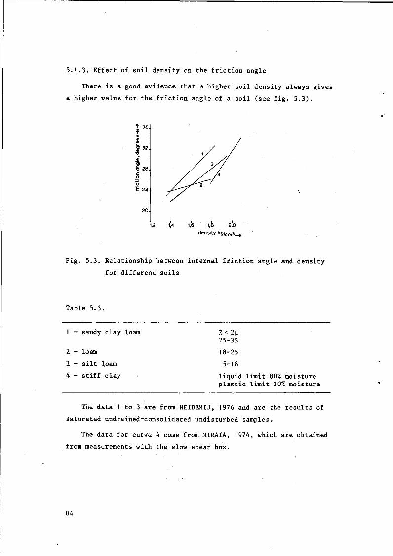
5.1.3. Effect of soil density on the friction angle
There is a good evidence that a higher soil density always gives
a higher value for the friction angle of a soil (see fig. 5.3).
t 36 ?
ff32
o 28
•fc 24
20.
1,2 1,4 1,6 1,8 2,0
density kg / c m 3_
Fig. 5.3. Relationship between internal friction angle and density
for different soils
Table 5.3.
1 - sandy clay loam
2 - loam
3 - silt loam
4 - stiff clay
%< 2y 25-35
18-25
5-18
liquid limit 80% moisture plastic limit 30% moisture
The data 1 to 3 are from HEIDEMIJ, 1976 and are the results of
saturated undrained-consolidated undisturbed samples.
The data for curve 4 come from MIRATA, 1974, which are obtained
from measurements with the slow shear box.
84
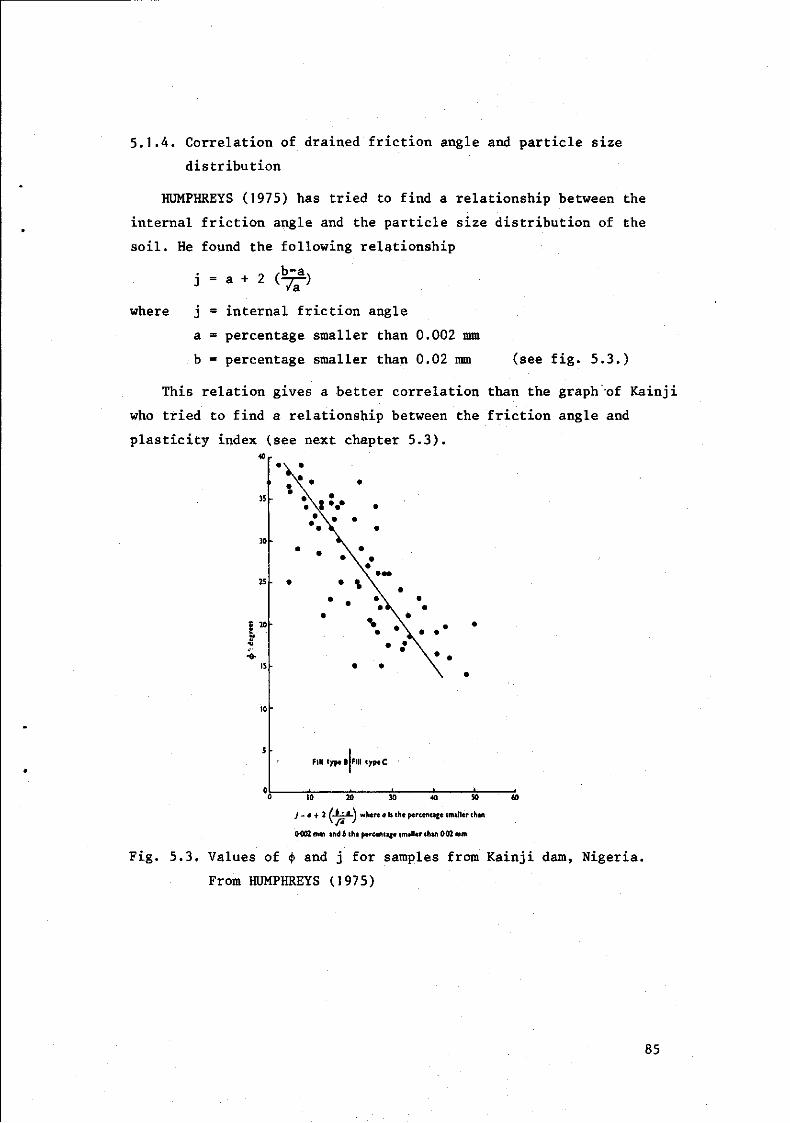
5.I.A. Correlation of drained friction angle and particle size
distribution
HUMPHREYS (1975) has tried to find a relationship between the
internal friction angle and the particle size distribution of the
soil. He found the following relationship
j = a + 2 (-75-)
where j = internal friction angle
a = percentage smaller than 0.002 mm
b = percentage smaller than 0.02 mm (see fig. 5.3.)
This relation gives a better correlation than the graph of Kainji
who tried to find a relationship between the friction angle and
plasticity index (see next chapter 5.3).
s » •a
Flll typ« 6 Fill typeC
10 20 30 « 50 (0
j ~ a + 2 l y ' a ) where a Is the percentage smaller than
0-002 mm and o the percentage smaller than 002 mm
Fig. 5.3. Values of <j> and j for samples from Kainji dam, Nigeria.
From HUMPHREYS (1975)
85

5.1.5. Correlation of drained friction angle and plasticity index
KAINJI (1974) proposed the following expression for the relation
between plasticity index and the friction angle measured at residual
strength
4 = 46.6/1 °' 4 4 6
P
where <|> = drained angle of internal friction
I = plasticity index, here from 5 to 50%
He found this relation from measurements of his own and that of
others (see fig. 5.4). 0Kenney(l959)
(D'SkemptonGibson-BJerrum'ln Bjerrum and Simoni (I960)
( ? ) Holt (1962)
( 7 ) Brooker and Ireland (1965)
©Mi tche l l (1965)
0 V o l t h t ( l 9 7 3 )
(7)Sollalone-peakva!uéi(ff„ = 0 l - (M I< l '™ l ) v— ' / Klnji
( ? ) Soil alone - peak values ( 0-„ = 3 5 k{/cm ' ) ( ( 1970, 1972)
( T ) Soil alone—minimum attained values (limited displacement)
Qo) Soil-polished rock Interface
40 60 Plasticity index, I f
° Bishop t.'al.(l97l) A Townstnd and Gilbert (1973)
d>r valuest g Tulinov and Molokov (1971) y O Kanji (1970, 1972), soil-polished rock
Fig. 5.4. Drained shear angle o> plotted against plasticity index I Ï
From KAINJI (1974)
Plasticity index is the moisture content between the liquid
limit and the plastic limit, here in percentage of dry weight.
86

5.2. C o h e s i o n o f c l a y o i l s
5.2.1. Cohesion and moisture content
Cohesion is taken here as the intercept of the Mohr-Coulomb
failure envelope with the shear-strength axis in the shear strength
normal load plot.
Fig. 5.5 shows the relation between cohesion as measured with the
triaxial test and the moisture content (see also table 5.4). There is
a good evidence that cohesion decreases with increasing moisture
content. The heavy clays have higher cohesion values than the more
sandy clays at the same moisture content.
40 44 48 moisture content
Todw—*
52
Fig. 5.5. Relationship between moisture content and cohesion for
different soils
Table 5.4
1. 2. 3. 4. 5. 6. 7. 8. 9.
10. 11.
Moraine Moraine Boulder clay Boulder clay Boulder clay Sandy loam Lean clay Residual clay Clayey loam Residual clay Heavy clay
% < 2y
< 1 2 4
10 19
+ 15 23 25 35 44 47
dry density gr/cm3
2.1 1.93 2.17 2.1 2.02
-1.36-1.48 1.16
-1.54 1.16-1.30
author
Bishop 1957 ii
H
II
H
Bekker 1969 W.E.S. 1964 Bishop 1957 Bekker 1969 Bishop 1957 W.E.S. 1964
87

5.2.2. Cohesion and soil density
There is no substential influence of the soil density on the
cohesion (see fig. 5.6 and table 5.5).
0.8 T J E
0,4i8
1,4 1.6 1,8 2,0 dry density g / c m 3_^
Fig. 5.6. Relation between soil density and cohesion for different
soils
Table 5.5. Origin of the data from fig. 5.6.
1. Silt loam
2. Loam
3. Sandy clay loam
%< 2y
5-18
18-25
25-35
author
Heidemij 1976
5.3. S h e a r s t r e n g t h o f c o h e s i v e s o i l s
5.3.1. Difference between peak strength and ultimate strength
Fig. 5.7 indicates the stress-strain behavior of a hypothetical
soil when carried well past the peak of the stress-strain curve.
This picture has been pieced together from the observed behavior
of a number of actuals soils. Some of the main features of this
picture are.
1. The postpeak dresp off in strength becomes more pronounced as the
degree of overconsolidation increases, but can be quite noticeable
even for normally consolidated soils.
88

Displacement Effective stress on shear plane
NC - normal consolidated
OC = over consolidated
Displacement
Fig. 5.7. Relationship between peak and ultimate conditions.
From LAMBE, 1969
2. In the ultimate condition the strength at a given effective stress
is independent of past stress history. In fact, the ultimate
strength of remolded and undisturbed specimens of a given soil
have proved to be essentially the same.
3. The strength envelope for the ultimate condition is a straight
line through the origin, generally at a position lower than that
for the peak strength of the normally consolidated clay.
4. In the ultimate condition the water content for a given effective
stress appears to be independent of past stress history. Actually
it is very difficult to establish this as fact, because the failure
zone tends to be very thin (perhaps only a few microns in thick
ness) and the water content of a slice cut from the clay may not
be representative of the water content in the actual failure rate.
Thus the overall behavior of clay is essentially the same as that
of sand: there is an ultimate condition wherein the strength and void
ratio are independent of past history. In this ultimate condition,
there really is a unique relationship among strength, effective stress
89

and density of packing.
However, there is one important difference between the ultimate
strength behavior of sands and clays: in clays the ultimate strength
can be significantly less than the peak strength of normally con
solidated specimens, whereas the peak and ultimate resistance of
loose sand are equal.
Although the progressive breaking of adhesive bonds may play a
role in the postpeak drop off of the strength of normally consoli
dated clays a second factor that would seem to be even more important
is the quadral reorientation of clay particles into parallel, face-
to-face arrangements.
Such reorientation should be accompanied by a decrease in <f>y and
also a decrease in the degree of interlocking. This reorientation
also seems to play a role with regard to the postpeak loss of strength
in overconsolidated clays, in as much as some of this loss seems to
occur after the clay has reached essentially constant volume.
There is good evidence that this reorientation occurs. Polished,
slickensided surfaces have been found in direct shear tests after
considerable strain.
Examination of failure zones using the electron microscope and
X-ray techniques has indicated a highly orientated fabric. Finally
it has been observed that the strength of clays at large strains
decreases while the void ratio apparently is decreasing slightly,
a phenomenon which can most readily be explained by reorientation.
5.3.2. Peak strength and ultimate strength for soils with different
clay content
Fig. 5.8 indicates the way in which the ultimate friction angle
varies with clay content. For clay contents approaching 100% the
ultimate friction angles are of the same magnitude as $\i for the
sheet minerals (<f>y = interparticle friction). For very low clay
contents if ult. is of the same magnitude as $\i between quartz par
ticles. In the general case, where the soil consists of both plate
like and granular particles, the granular particles tend to raise
<t> ult. above <jjy for the clay particles by inhibiting to some extent
the full orientation of the clay particles and by contributing some
90
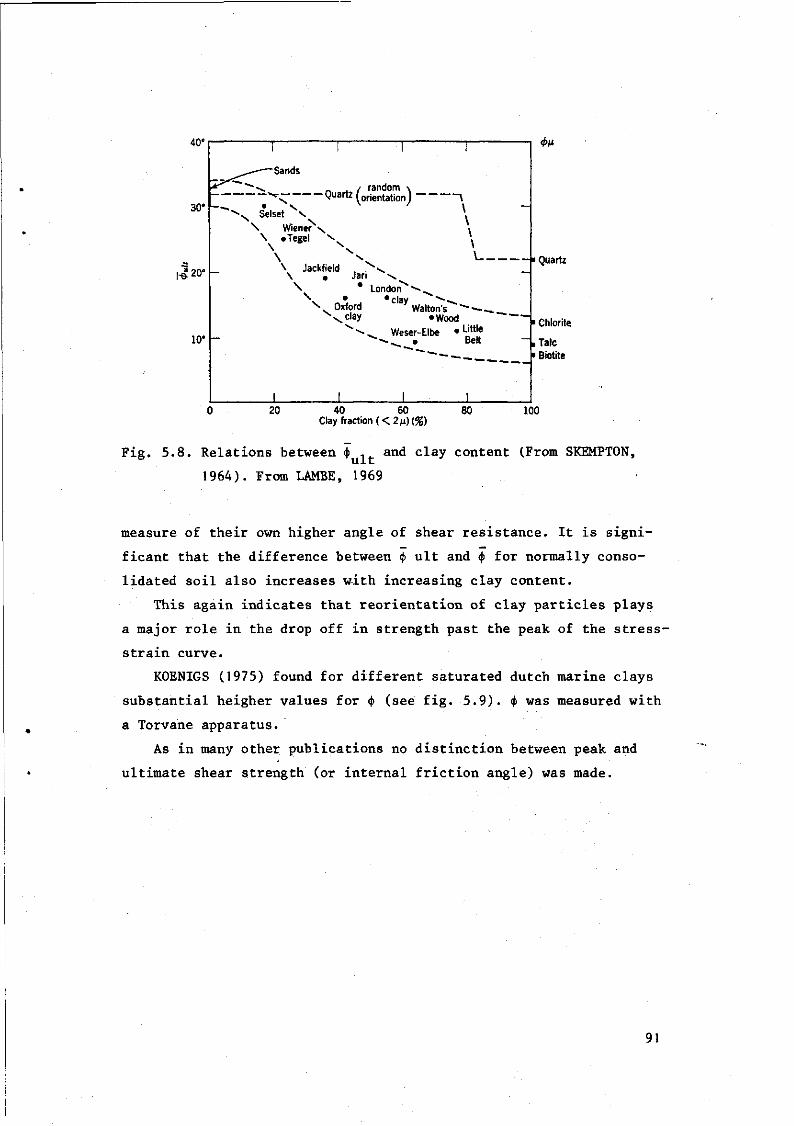
40'
30*
I-&'
10°
•Sands
/ random \ r ^7 Quartz (orientation )
• x * N Selset N.
\ Wiener̂ \ \ «Tegel V
—\
\ Jackfield \
\ — • Quartz
Jari \ * London
V n \ j 'clay x Oxford ' % v C l a y
Walton's " - — •Wood
Weser-Elbe • L i t , l e
^ • Belt
«AM
• Chlorite
• Talc • Biotite
20 40 60 Clay fraction ( < 2 M ) (
80 100
Fig. 5.8. Relations between <j> - and clay content (From SKEMPTON,
1964). From LAMBE, 1969
measure of their own higher angle of shear resistance. It is signi
ficant that the difference between 4> ult and $ for normally conso
lidated soil also increases with increasing clay content.
This again indicates that reorientation of clay particles plays
a major role in the drop off in strength past the peak of the stress-
strain curve.
KOENIGS (1975) found for different saturated dutch marine clays
substantial heigher values for <j> (see fig. 5.9). $ was measured with
a Torvane apparatus.
As in many other publications no distinction between peak and
ultimate shear strength (or internal friction angle) was made.
91

6?]
54
4b
38
30
t Jt 4»
4) •D
• 0) O) c o c o
. V» u
' t -
\ x
X \
\ x
X \
1 . . I . f r -
20 40 60 80 100 °/.<2H-»
Fig. 5.9. Influence of clay content on the friction angle.
From K0ENIGS, 1975
5.3.3. Effect of soil moisture content on the shear strength
VENEMAN (1976) found the relationship between soil moisture and
shear strength (see fig. 5.1C and 5.11)
z O | 3 0
£251 z O u
£20
§15}
10 '
VANE SHEAR rsO.44 «=0.77 •BATAVIA 60CM oBATAVIA 120CM «MIAMI 60c»
X=6.72 - 0.154 Y
«P-r 2 — 3 — t — s — 8 — r SHEAR STRENGTH (KIPS / SQ FT)
-ft , - -2 r SHEAR STRENGTH (KG / SQ CM)
Fig. 5.10. Soil shear strength as measured with the vane shear test
as a function of the soil moisture content (weight % ) .
Fron VENEMAN, 1976
92

X o E30
£25
" 2 0
Ï 1 5
10
-r
UNCONFINED COMPRESSION rz0.63 « = 0.115 • BATAVIA 6 0 CM o BATAVIA 120c« > DATA IGNORED IN
REGRESSION ANALYSIS
= 1 3 . 2 3 - 0 . 4 3 7 Y
•ft-. SHEAR STRENGTH (KIPS/SQ FT)
- * , • S
- a — s — 8 — r •3"
SHEAR STRENGTH (KG/SQ CM)
Fig. 5.11. Soil shear strength as measured with the unconfined com
pression test as a function of the soil moisture content
(weight % ) . From VENEMAN, 1976
The soil tested was a silty clay loam (LL< 50%). They found a
multiple regression equation for the shear strength as measured in-
situ with the vane shear apparatus.
where
X = -3.84-0.18 ew+0,47U-0,4PI
2 X = in-situ shear strength (Kips/ft )
ew = moisture content (weight %)
LL = liquid limit (%)
PI = plasticity index (%)
Inclusion of bulk density and clay content in the equation im
proved the correlation coefficient with only a factor of 0.029 which
can be neglected.
P0TAP0V (1966) found the following results from measurements with
a Tolstoy apparatus with soil sample of 40 x 60 x 5-7 mm. The soil
tested was a Sod-Podzolic (fine clay loam) - devided into two parts
(47,95%<0,01 mm - 12,8% < 0,001 mm)
I macrostructural samples - fractions 1-2 mm and< 25 mm
II microstructural samples -< 1 mm (for results see fig. 5.12)
and a chernozem (fine clay loam, 71,76%< 0,01 mm and 43,73%< 0,001 mm)
(see fig. 5.13)
93

m 3o ~w so Moisture content W, %
Fig. 5.12. Change in the maximum shear strength of samples of Sod-
Podzolic soil as a function of moisture content.
Microstructural samples: 1) during drying process; 2) du
ring wetting process. Macrostructural samples: 3) during
drying process; 4) during wetting process.
From POTAPCV, 1966
Fig. 5.13. Change in the maximum strength of microstructural samples
of Chernozem soil as a function of the moisture content.
1) during drying process; 2) during mechanical compaction
after wetting; 3) during wetting without additional com
paction. From POTAPOV, 1966
94

He ran two series, one in which the samples were wetted to a
moisture weight of 17,5-57,0% and one in which the samples were
first wetted and then dried at 25 C to the desired moisture content.
Whenever microstructural samples are dried to a moisture content
of 17% or less we see a decrease in the maximum shear strength as
the result of the appearance of microtracks, which are noticeable
in a twofold magnification.
For the Sod-Podzolic the compaction of the macrostructural samples 3
vary between 0.82 and 0.85 g/cm , the compaction of the microstruc-3
tural samples vary between 0.98 and 1.06 g/cm under a load during 3
the wetting process, but between 1.06 and 1.21 g/cm during the drying process.
Compaction during drying gave a higher shear strength than mecha
nical compaction to the same density. Compaction during drying of 3
chernozem soil varied between 1.01 and 1.14 g/cm while the mecha-3
nical compaction was stopped at a density of 1.10 g/cm .
5.3.4. Physiochemical effects on the shear strength of clays
OLSON (1974) studied the influence of ion concentration on the
shear strength of kaolinite, illite and montmorillonite.
The terms "physical" and "chemical" may be applied rather loosely
to describe the interaction of particles. The term "physical" is used
to denote interactions that are controlled largely by the size, shape,
packing and physical properties of the individual grains and to the
friction between them, whereas the term "chemical" is applied to
interactions through diffuse double layers, van den Waals forces,
and ionic forces.
For the three clay minerals studied the shearing strength appeared
to be controlled mainly by the physical effects. No diffuse double
layer effects were apparent for any of the clays in the calcium form.
For clays in the sodium form no diffuse double layer effect was
noted for sodium illite.
For sodium montmorillonite the strengths were so low that re
ductions in normal effective stresses of 50% or more would probably
go undetected.
95

Taken collectively the data suggest that location of the
effective-stress failure envelope is controlled mainly by physical
effects controlled by the size and shape of the individual particles.
Particles that are large and more or less equidimensional lead
to high strengths regardless of chemical effects, whereas particles
that are very thin with high diameter-to-thickness ratios, as in
sodium montmorillonite, have very low strengths.
The values of <̂ R were similar to the residual values of <}> re
ported by Kenney (see OLSON, 1974). For a summary of the test re
sults see fig. 5.14 where R denotes consolidated-undrained test and
S consolidated-drained test.
30
20
1-6- 10
•
•
AO
Koolimte
A
A
o A
O
•
• •
•
Iff 1 i
lllite
v. Montmorillonite
from R triaxial compression tests
droined direct sheer tests by Kenney (II)
sodium saturated
calcium saturated
undefined
Fig. 5.14. Comparison of friction angles measured using R triaxial
compression tests with residual angles measured using S
direct shear tests on thin samples. From OLSON (1974)
The soil under investigation had following properties (table
5.6).
96

•o u 01 eu u u cO 01 B E
• H es u - r l co - o w
n c 0) CO C J3
•H 4J Ph
1
> • H
C 3 •H er
n QJ U -.H W rH U rH
• H
E
0) ^i co CI) H S eu e r 4-» CO QJ
- e
u J 3 OD
• H CU
X
CO
CO M
M
3-CN
( H
CU
a CO 4 J
fi CU r H
«
h eu a
0 • H ^ 4J CT\ es ^ -^ )-i
eu s e * 4J
c •-• eu oo u -^ u eu a.
0 0
,—* O r~ O —'
—
e en ^ U >x> 00 ~y
LO 1
CN
r^ < f
i n •
o-l
m
• r -
< j
—•
O u- l
1 O
—
o o r -
i n CNl
O O •—I
1
o c^
o o m i
o m r -
r*-o\
O O
—
O
o r^
1 O
o m
o 00
CU eg oo
et) co u ce) C
eu « o
•J1* ^ 3 eu P.
eu co oo
co CO 4J
co c CU
- o •4 IH
3 <u p.
! s f V
-—* m
*—̂
— •
en 1
p-* CN
O m l
o < f
o -3-1
i n m
o o
1 m -X)
r-~ - 3 -
1
~-m
o vO
— « •— l o <y*
—
z o co • J
o
§ u
Pu
eu p. o u
o co
cO
H
CU o U CU
3 B O CO co e
» CU ^"* U T) N CU CO - - '
•H U rH 4J o. a-o 3 c
c o co
X d j
co r - f co O
• r l
e CU J 3 O
• O CS CO
co T-H co h eu B
• H
S
* CO ••H 0 0 U o eu
Ü
•» eu M
>-. 4-1 C
l - l O
S r.
• P. h O
CJ
s* es
i - i CJ
eu
^ >> •o C O
r H
*:
CO • H 0 C
• H r H f - l H
* C eo
• H - C 4J
• iH
fc,
« • cS CO
•a ^ •H CS 0 rH
rH Ü rH rH O o o > c » CO 00 CJ C
• r i - H r i S CU O
J£
eo U /-* eu — fi ^
• H
O cS
O
S c o g
u • H
R • r ) r H
T ) • H 3 cr
• H r H
II
• J S
eu M eu
X 3
4J • H
R • H r H
CJ • r i U C0 es
t~t
a n P H
3
R CJ
— u on
:* 4-1 • r t en C eu
• O
II
O
97
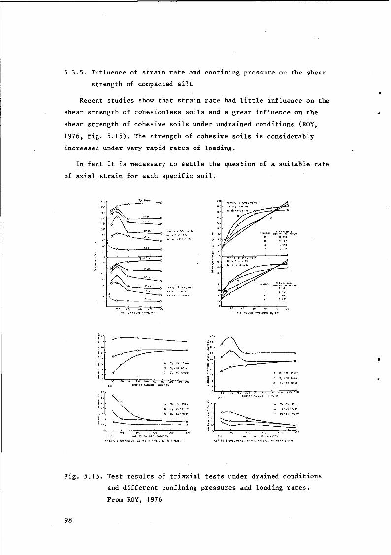
5.3.5. Influence of strain rate and confining pressure on the shear
strength of compacted silt
Recent studies show that strain rate had little influence on the
shear strength of cohesionless soils and a great influence on the
shear strength of cohesive soils under undrained conditions (ROY,
1976, fig. 5.15). The strength of cohesive soils is considerably
increased under very rapid rates of loading.
In fact it is necessary to settle the question of a suitable rate
of axial strain for each specific soil.
- • ' " C
k •-' j ^ P ^ £a c
; , ^ - - O O — O
jCO 400 50C 60 BO
All HOUND "*fSVURE T-,,
SO 100 ISO ?00 ?50 J00 KO iOO <•« 50C
i p TIME 10 F4IIUBC - M1NUT65
\ o
*^H .
fl 3
O
,
T . •">
T% . )'•
<T> '6C
10 P*
h?.:*
•?0PI
n
Ci TUE TO FAILURE - MiNU'ES
SE»'É5 * V f CIMENT" *v M C - i l ' X , AV it t " l W i l l
ijo SI-J ÎSC Ir/j Ac -V. TTTTio ME T0 fA - ' - " f - '
bEOlES a SPECIMENS. *« M r. • H 5 \ | AV in • i " fc >c - it
Fig. 5.15. Test results of triaxial tests under drained conditions
and different confining pressures and loading rates.
From ROY, 1976
98

Table 5.7. Characteristics of soils tested
silt fine sand < 2^
silty soil 85 % 10 % 5 %
mean particle size 0,01 mm
liquid limit = 34,6 %
plastic limit = 17,6 %
specific gravity =2.67
Samples were compacted, following Standard Proctor test procedure at 3
a dry density of 1860 kg/cm .
The fig. 5.15 (6 en 7) shows that cohesion decreases andiangles
of internal friction increases with decreasing confining pressure.
For the soil drier than the optimum the same trend also persists
with increasing test duration arid the rate of change in c and <j> goes
on decreasing with decreasing cell pressure until at a confining 2 2
pressure range of (103,5 kN/m - 207 kN/m ) the shear strength para
meters are practically uneffected by the speed of shear; c and <j>
remain virtually constant beyond the test duration of 200 min. at
this pressure range. For soil wetter than the optimum the degree of
saturation is high and at lower confining pressures (103,5 - 414 kN/ 2
m ) range drainage appears to be poor at the faster rates of strain
in variation of c and <j> with speed erratic. For higher confining
pressures the failure zone of the samples probably becomes fully
saturated and with increasing test duration ç and <|> approach their
drained values in a systematic manner.
For failure times greater than 200 min. variations in the values
of c and <(> with increasing failure time are similar for soils both
drier and wetter than optimum. The 500 min. tests appear to be fully
drained, i.e. at failure the shear parameters tend to reach identical
values irrespective of whether the samples were initially drier or
wetter than optimum.
5.3.6. Hyperbolic function to describe the stress-strain relation of
compacted clays
DANIEL and OLSON (1974) found that the hyperbolic curve originally
99

used by Kondner fit the data of the triaxial stress'-strain curve
better than any other simple expression.
Kondner's expression is of the form
0-1-03 = — (1) a + b ca
al-o3 = stress difference
ea = axial strain
a and b = constants.
The constants a and b can be found by rearranging eg. 1 to
e a = a + bea ' (2)
where
al-a3
and then plotting ea/al-a3 versus ea. If the hyperbola (1) describes
the stress-strain curve accurately, then the experimental data
should all plot on a single straight line in the transformed plot
with intercept a and slope b.
Another method for finding a and b is to fit the hyberbola
through two points on the stress-strain curve where the stress dif
ference is equal to 70% and 95% of the peak stress difference.
Physical significance of Kondner's constants.
Kondner demonstrated that constants a and b have a physical meaning,
i.e. a is the reciprocal of the initial largest modulus and b is the
stress difference to which the hyperbola becomes asymptotic at in
finite strain. Kondner noted that the experimental stress difference
at failure is somewhat less than the stress difference to which the
hyperbola becomes asymptotic and presented the following hyperbolic
equation
Ea oi-o\3 =
-L+ Rf va (3)
Ei (al-a3)f a
where
Ei = initial tangent modulus
(al-o3)f = the experimental stress difference at failure
Rf = failure ratio which is defined as the ratio of the
experimental stress difference at failure to the
reciprocal of Kondner's constant b.
100

Influence of confining pressure.
To use eq. 3 to approximate the stress-strain curves of compacted
soils it is necessary to express Ei, (al-a3)f and Rf as analytical
functions of such independent variables as compaction water content
and confining pressure, with soil type and compaction procedure held
constant.
Correlation of Ei with confining pressure.
Janbu developed the following equation for the relationship between
El and a3: see DANIEL (1974)
Pa K CPa} (4)
in which Pa = the atmospheric pressure expressed in the same units
as a3 and Ei; and K and n are dimensionless constants. The equation
is in such a form that a plot of log Ei/Pa versus log (a3/Pa) for
the experimental data should define a straight line.
A typical plot of log (Ei/Pa) versus log (a3/Pa) is presented
in fig. 5.16 for a wide range in compaction water contents.
1 1 1 — I 1 I I T
Fig. 5.16. Log Ei/Pa versus log (a3/Pa) for a wide range of com
paction water contents.
From DANIEL (1974)
101

Eq. 4 apparently accounts for the variation of Ei with confining
pressure and compaction water content with reasonable accuracy. Note
that Ei in fig. 5.16 is the reciproval of Kondner's a coefficient,
not an Ei measured from the experimental curves. The values of K and
n may readily be evaluated from plots such as fig. 5.16. The value
of K is numerically equal to the value of Ei/Pa when a3/Pa=l and n
is the slope of the line of best fit.
Correlation of stress difference at failure with confining pres
sure. 2
For confining pressures smaller than about 100 psi (7 kg/m ) (.al-a3)f
is approximately a linear function of the confining pressure fig.
5.17 and the strength may be expressed by
(al-a3)f = d + a3 tan 4> (5)
in which d = the intercept; and <|> = the slope of the failure enve
lope.
200
- 100 -
—F .... ? ,., , Test Series 65 / «opi • , 5 % /
<ijr
Jjf - * ^
f w > 17% .
i '
-
40 80
a, (psi)
120
Fig. 5.17. Failure envelopes for confining pressures smaller than
100 psi (1 psi = 6.89 kN/m2). From DANIEL, 1974
The slope of the failure envelope usually decreases as the com
paction water content increases (fig. 5.17), but the intercept has a
maximum at a water content just dry of the optimum water content
(fig. 5.18).
102
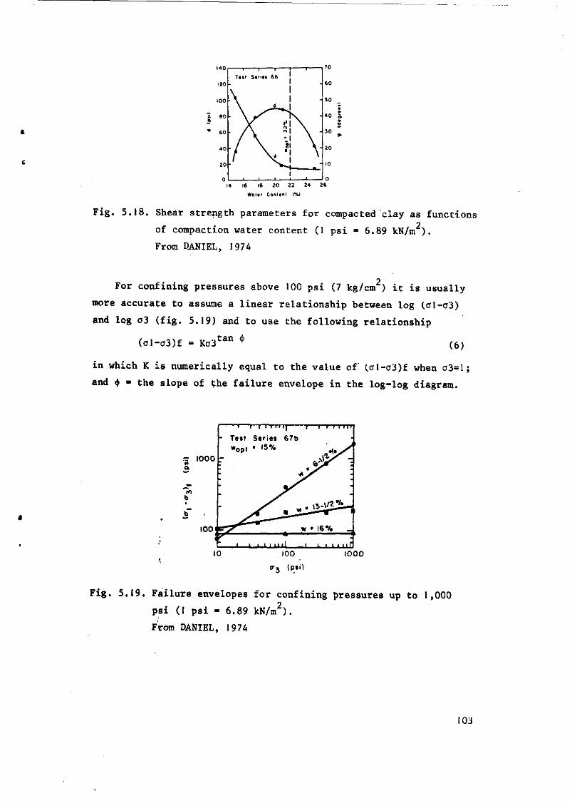
16 18 20 22 24 2G
Wal«' ConHnl (V.)
Fig. 5.18. Shear strength parameters for compacted clay as functions
of compaction water content (1 psi = 6.89 kN/m ).
From DANIEL, 1974
o For confining pressures above 100 psi (7 kg/cm ) it is usually
more accurate to assume a linear relationship between log (ol-o3)
and log 03 (fig. 5.19) and to use the following relationship
(ol-o3)f - Ka3tan * (6J
in which K is numerically equal to the value of (al-o3)f when a3=l;
and <{> - the slope of the failure envelope in the log-log diagram.
r= 1000
b
100
i 'I—I i i M i | 1 i i i 1111
Test Series 67b
*opt " l 5 %
1000
o-* (psi)
Fig. 5.19. Failure envelopes for confining pressures up to 1,000
psi (1 psi - 6.89 kN/m2).
From DANIEL, 1974
103

DANIEL (1974) supports the recommandation of Hunter and Chang
that Rf can be teken as a constant equal to 0.9.
So the stress-dependent hyperbolic equation may now be written
as follows
o 1-0-3 = Ea 1 0.90
KPa(? ) n + d + a3 tan*
(7)
"Pa'
for the case of a linear failure envelope.
Fig. 5.20 shows some examples of fitting the hyperbola to the
experimental data.
10
•
•ƒ
T—
• •
Senes 69 _ * « 19% i ,
«opt * ' 8 ^
»3 " 5 p " ? (35 kN/itiM
; '5 a.
b
1 '0
(T
i
•/ Stf
•̂ Ä
e> 6 Î 3 %
<**^>
9
• op l • l»%
» 3 • 5 • " ' , 135 kN/m<>
• i
w • 2 5 % 1 w o p t • 2 2 %
<r3 * GO B»<
( 4 2 0 h N / m 2 l
5 10 15 20 10 15 Z0 10 15 20
o CM
Fig. 5.20. Examples of 'poor', 'average', and 'good' correlations
between theoretical and experimental stress-strain curves
(1 psi = 6.89 kN/m2).
From DANIEL, 1974
The test procedure used here was the unconsolidated-undrained
triaxial test on homogeneous and isotropic compacted specimens.
DANIEL (1974) describes also analytic expressions for Poisson's
ratio, i.e. the influence of axial strain and confining pressure on
Poisson's ratio.
104
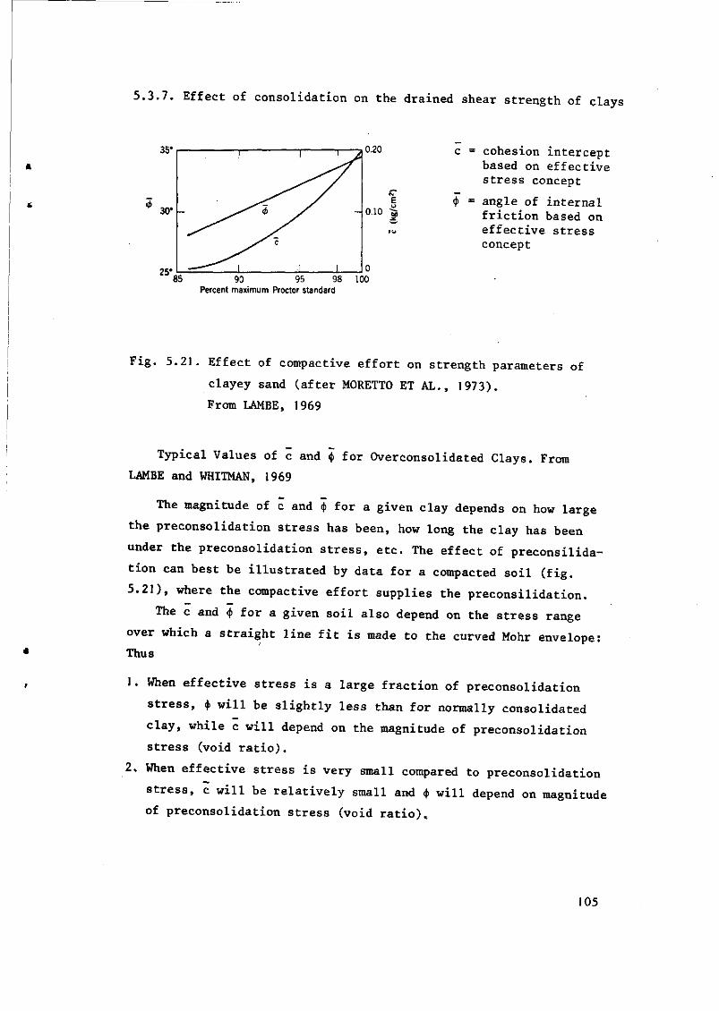
5.3.7. Effect of consolidation on the drained shear strength of clays
0.20
0.10
C =
90 95 98 Percent maximum Proctor standard
100
cohesion intercept based on effective stress concept
angle of internal friction based on effective stress concept
Fig. 5.21. Effect of compactive effort on strength parameters of
clayey sand (after MORETTO ET AL., 1973).
From LAMBE, 1969
Typical Values of c and <£ for Overconsolidated Clays. From
LAMBE and WHITMAN, 1969
The magnitude of c and <j> for a given clay depends on how large
the preconsolidation stress has been, how long the clay has been
under the preconsolidation stress, etc. The effect of preconsilida-
tion can best be illustrated by data for a compacted soil (fig.
5.21), where the compactive effort supplies the preconsilidation.
The c and <|> for a given soil also depend on the stress range
over which a straight line fit is made to the curved Mohr envelope:
Thus
1. When effective stress is a large fraction of preconsolidation
stress, <)> will be slightly less than for normally consolidated
clay, while c will depend on the magnitude of preconsolidation
stress (void ratio).
2. When effective stress is very small compared to preconsolidation
stress, c will be relatively small and <\> will depend on magnitude
of preconsolidation stress (void ratio).
105

Fig. 5.22 illustrates (to an extreme degree) the way in which
c and <j> can vary with the stress range. The Mohr envelope for an
overconsolidated soil seldom is as that in fig. 5.22.
Usually the <|> from a straight-line fit to an overconsolidated
clay is about equal to that for normally consolidated specimens.
Moreover, the effects of preconsolidation on strength are important
numerically only at small effective stresses; at large effective
stresses the envelopes for normally and overconsolidated specimens
of a clay tend to merge. Thus the major question with regard to
overconsolidated clay lies in choosing the appropriate value of c. 2
Values of c ranging from 0,05 - 0,25 kg/cm are often used for soils.
Even larger values undoubtedly are valid for the stiffest of soils,
but large "measured" c values frequently result from running CD tests
too rapidly so that pore pressures develop. Extreme caution must be
exercised when choosing a value of c for practical calculations.
400
300
=• 200
100
! : i ! 1
i : i
1 !
^ - < 1 ) c = 18 ps . ^ 1 l</> = 26°
i
c= 113 £=10"
i l 1 j
i
psi
h- • • I
200 400 600 800 1000 ä[f (lb/in.2)
F i g . 5 . 2 2 . S t r e n g t h e v en l ope f o r unwea the red London c l a y (from
BISHIP, ET AL. , 1965 ) .
From LAMBE, 1969
106

5.3.8. Influence of soil density on the shear strength
ANDERSON (1976) gave the values shown in fig. 5.23 for the
shear strength of soils with different density.
shear strength kg/cm2
3.6 r
3.2
2.8
2.4 -
2 . 0 -
1.6
1.2 -
0 .8
0.4
• 2
• 13
• 6
• 14
• 7
• 5
• 1 • 3
I * 1 5 I I I
• 10
•12
• 9
• 8
J L 1 4 15 16 17 18 19 2 0 21 2 2
density kg/cm3
Fig. 5.23. Relation between shear strength and density.
From ANDERSON, 1976
The data are taken from table 5.7. There seems to be a relation
between density and shear strength. Due to the different test methods
used in table 5.7 it is very dangerous to establish relationships
between shear strength and other soil parameters such as clay content,
soil density, etc. from these data.
107

oo G
•o eu CU u G u
•H 01 cd
01 J3 -a-eu 4-» —
H CU ^
6
P. E co • o — o
300 - - ' c/l ,Ü
C U • H cu co / -N - *
o , ß CM • o — — l
cjoo --• eu M
00
o
CJ 3 •a cd
C/l
>
co i n v£> <f cr\ - j - r~- i n oo i n
o — i o o I O O O co CM i —
o a\ o co r^ CM
I N i n - N l
o
d i
O c j
•O G I cd
c j
CJ 3
C/2
> • 8
U I
O 1
CM
0 0
1 CM
CM
— O 1
CM
1 O 1 1
-3-
c o I I I I o I I I
cu
a
e CU
TS u 3 & U CU > o
s cu <u co cd 3 . — —
OO t l £ CM cd t-A
G I co •H «H w /-*
H I O •* i—I 4-t •—> O M CO —' m s E
CU co I 00 cd H cd .—^
CU 4J CTV » O. e •^ Çh CU
M cd O
CO CU cd I oo
» CU 4J 00 — a e v^ — CU
S cd u
oo
o o o
CM
co O O
co -»
CJ1 — KO • J - I A CM
CM CM CT* O O O O O O
i
l
< — V
CM
O
/—•. /^N ^ O
r» co o —
CM o o r-» <!• - 3 - i n C M
m c o < • CM O O O r -O O o O
*"*
CM
S
CM
O 0 0 C M r>-
018
0005
O C O O O
er. - j - c M m o o er. r- o o C O I I vO I CM I CO I — — CM — 1
0 > 0 - J CO CO -et
r^ i n o i n co co <f CN
O -3-— -3-
m <j\ CM VO I
m in
o o
o o
»3- O i m m
a\ m oo oo
co 00
• a eu
o • i t o
O
1
vO CM
O
o
-a-CM
O
O
CU
u cd
• o CU
u cd
TJ •H t - t O coco G e 0 — o oo
CU co I 00 nj u cd .-N
a) 4J N * o, G " - ' — eu
Dl « O
CO vO
• WCO u cu E oo P, o
r ~ r - - o o o o c M c o o r - ~ - j - o o o — o o ^ o r - o o ^ o r ^ c o i n o r ^ C A O O O O O C A C i O C f l C h O O O C O O O — — — — — - . _ — _
> * * r f I ~ " VAS * * * I ^ * l « 1 V—J 1 ^
i t X 3 C T . C T \ c y . a \ C T \ e j \ O C X i t
I I I I I
vO oo er. oo CT. ON CT. CjS
I • I
v û r ^ - o o o m m <f co r» vo -a* co m \ o I N co vo cftco tn r ^ r ^ m * £ > m c 7 \ C 3 ' \ r ~ - o o ^ o c M C T > o o — CMCM — i n i n m i n r ~ i - * - . m m O cj\ o\
u o u cd —
co E
eu m C o cd co > •
o C M C M C M C M C M C M
o en
W
CO H
e co u •H T3 H 'M *J ^
e cu .o eu m * 3 O, 3 CU ^
O CJ CM t^ o .
CU -3-
4-1 CU CO £1 ^ N eu S co H 3 ^
C
cu » i-H J3 4-1 CU -U C CU / -v g O, . H CU CM Cd CU U-t ^
CO " 3
o — er. — — o\
o r ^ o c j v c T . m m r ^ c o o o v o c M o o o o — r ^ o o m v û O c M v û r ^ O C n c M — O — - O — CMCMCMCOCOCOCOCT\OCy.CT. — — o \ o \
— o > c o r N — ( j . c N v j c ^ i n c o i o c s i O v O - f f . o ^ t ^ - c o i o r i N c n c o
— ' O C O C O O C O C O N O v J C O N \ O N v t v J ( O i n - o — o — ~ — CT*
_ „ ' „ « N O O - — — O O O O O O O O C M C M C M C M — — CM —
_ _ cd .a JS " - * C ^ S M I I ? ? C M - C M C O - C M - T J J 5 C O C M 5 2 - C M ^ ^ S ë S ^ 2 2 c o c o ' ^ ^ w « " u " " 3 3 ^ ^ S S s s
™ m Pd ai y
I o < r « « O N — ~ CM CM CO
\ 0 < r o — m m — m m v ß r ^ it — CMCMCOCOm — — — —
r- l CU r l S - - N o cd —
J l Ö ^ i—t r-t 01
PO
| CU CU
u U 4 • H - H CJ
ß C -H • H O i -< r-4 4J « H o C cn es cu
4J • H > , O cd h r-< 4J CJ CU
o
>̂ >. >^ cd cd Cd r H t - t
i - I O CJ CJ
a >. T 3 O > h u « o cd x
fn W O
cd
•o CU
cd
cd
cu
I X cu >, i S cd M
i-i cd I H o oa o
o co cu o
3
— — — 4J
CM O O O
— — CM CO
<!
i n vo vo co CM — — CM
cd u
- * G xi
i-H !>> oo cd
o) ca
o G & O
CO t 3 CU O
V
U G i-i
cd
co co cu CM
CU e o ü - i l c w a 3 U .H E3 TJ T3 o eu eu H B CO
CU -H 3 td
cd M U T3 cd C cd
oc >e! -H cd i u
n)
108

5.3.9. Values of the c and <t> (from undrained consolidated triaxial
tests)
Soil clay content dry water cohesion friction density content kg/cm^ angle gr/cm^ % dry weight c degrees
Moraine
Moraine
Boulder clay
Boulder clay Sandy loam
Boulder clay
Lean Clay
Residual clay Clayey clay
Residual clay
Heavy clay
< 1
2
4
'0
10
19
23
25
28H40
44
47
2.1
1.93
2.17
2.1
-
2.02
1.48 1.50 1.41 1.36 1.16
T
1.54
1.30 1.32 1.22 1.16
6.8 8.8
10.2 9.6
12.2 14.8 6.8 7.8 8.8 9.5
12 16 20 24 8.8
10.7 12,4 22 26 30 32 48.2
38 42 46 51 20 23 25 25 35 40 45
0.43 0.37 0.056 0.7 0.48 0.0 0.64 0.48 0.13 0.7
0.07 0.14 0.12 0.07 1.15 0.81 0.24 0,49 0.42 0.26 0.14 0.59
0.035 0.053 0.059 0.039 1.27 1.103 0.30 0.50 0,30 0.16 0.10
42 44 41 36 37 36 38 38 37 33
32 28 24 18 27 24 28 18 6 0 0
31
14 15 16 10 24 21 24 12 1 0 0
109

LITERATURE FRICTION ANGLE, COHESION AND SHEAR STRENGTH CHAPTER 5.
OF COHESIVE SOILS.
ANDERSON, DONALD G. and RICHARD D. WOODS. Time-Dependent Increase
in Shear modulus of clay. Journal of the Geotechmcal Engi
neering division. No. 5 - 1976, p. 525-537.
BEKKER, M.G. Introduction to Terrain-Vehicle Systems. University of
Michegan Press, Ann Arbor 1969
BISHOP, ALAN W. and D.J. HENKEL, 1957. The measurement of soil pro-
perties in the triaxial test. Edward Arnold (Publishers)
L.T.D. London.
DANIEL, David E. and ROY E. OLSON. Stress-Strain Properties of Com
pacted Clays. Journal of the Geotechnical Engineering Divi
sion, no. 10 - October 1974.
HEIDEMIJ. Bodemkundig-Grondmechanisch rapport. Rapport nr. 667-76/3.
Hoofdwatergangen in de ruilverkaveling Voorne-Putten.
Dienst voor de landinrichting in Zuid-Holland.
HUMPHREYS, J.D. Some empirical relationships between drained friction
angles, mechanical analyses and Atterberg limits of natural
soils at Kainji Dam, Nigeria. Geotechnique, vol. 25, no. 3 -
sept. 1975.
KAINJI. The relationship between drained friction angles and Atten-
berg limits of natural soils. Geotechnique, vol. 24, no. 4 -
dec. 1974, pp. 671-674.
KOENIGS, F.F.R. Apparent volume and shear strength of consolidated
submerged sediments. Geotechnique 25, no. 2, pp. 265-278.
LAMBE, T. WILLIAM and ROBERT V. WHITMAN. Soil Mechanics Massaschu-
setts Institute of Technology, 1969. John Wiley and Sons,
Inc., New York.
MIRATA, T, The in-situ wedge shear test - a new technique in soil
density. Geotechnique 24, no 3, pp. 311-332.
OLSON, ROY, E. Shearing Strengths of Kaoline, Illite and Montmoril-
lonite. Journal of the Geotechnical engineering division,
no. 11 - november 1974.
P0TAP0V, B.I. Influence of moisture content and soil compaction on
the soil's maximum shear strength - Soviet Soil Science -
april 1966, no. 4, page 396.
110
ROY NIKHILESH and PANTH SARATHI. Strain Rate Behavior of Compacted
Silt. Geographical Vol. no. 4, april 1976, p. 347-360.
VENEMAN, P.L.M., J. BOUMA and T.B. EDIL. Soil shear strength varia
tion in soils of a Bavaria Silt loam mapping unit-
Soil Sei. Soc. Am. J, Vol. 40, 1976.
V0M0CIL, J.A. and W.J. CHANCELLOR, 1967. Compressive and Tensile
Faiure Strengths of three agricultural soils. Transaction
of ASCE 1967 Vol. 10, no. 4.
W.E.S. U.S. Army Engineering Waterways, Experiment Station Technical
Report no. 3-639. Corps of engineers. Vicksburg, Mississipi,
January 1964.
J
111