ON TRIVIAL WORDS IN FINITELY PRESENTED GROUPSandrewr/pubs/trivial_words.pdfIn this article we consider the function that counts the number of trivial words in a nitely presented group,

ON TRIVIAL WORDS IN FINITELY PRESENTED GROUPS

M. ELDER, A. RECHNITZER, E.J. JANSE VAN RENSBURG, AND T. WONG

To the memory of Herb Wilf, Pierre Leroux and Philippe Flajolet — all great men of generating

functions.

Abstract. We propose a numerical method for studying the cogrowth offinitely presented groups. To validate our numerical results we compare them

against the corresponding data from groups whose cogrowth series are known

exactly. Further, we add to the set of such groups by finding the cogrowthseries for Baumslag-Solitar groups BS(N,N) = 〈a, b|aN b = baN 〉 and prove

that their cogrowths are algebraic numbers. We have been unable to find thecogrowth series for other Baumslag-Solitar groups, but we have found recur-

rences that yield the first few terms of the cogrowth series exponentially faster

than is possible by naive methods. Finally we apply our numerical methodto several presentations of Thompson’s group F and our results give strong

indication that the group is not amenable.

1. Introduction

In this article we consider the function that counts the number of trivial words ina finitely presented group, the so-called cogrowth function. The exponential growthrate of this function is simply called the cogrowth and is intimately related to theamenability of the group [12, 19]. Amenability is an active area of current research,and cogrowth is just one of many characterisations. The amenability of one groupin particular – Richard Thompson’s group F – has been the subject of intensiveresearch and conjecture.

In this article we propose a new numerical technique to estimate the cogrowthof finitely presented groups, based on ideas from statistical mechanics, which weshow to be quite accurate in predicting the cogrowth for a range of groups for whichthe cogrowth series and/or amenability is known: these include Baumslag-Solitargroups, a finitely presented relative of the Basilica group, and some free productsstudied by Kouksov [26]. We apply the method to several different presentationsfor Thompson’s group F , and the evidence obtained points strongly towards theconclusion that F is not amenable.

The present article builds on previous work of a subset of the authors [14], wherevarious techniques, also based in statistical mechanics, were applied to the problemof estimating and computing the cogrowth for Thompson’s group F . This in turnbuilt on previous work of Burillo, Cleary and Wiest [8], and Arzhantseva, Guba,Lustig, and Preaux [3], who applied experimental techniques to the problem ofdeciding the amenability of F .

Date: March 2012.

2010 Mathematics Subject Classification. 20F69, 05A15, 60J20.Key words and phrases. Cogrowth; amenable group; Metropolis algorithm; Thompson’s

group F ; Baumslag-Solitar group; cogrowth series.

1

2 M. ELDER, A. RECHNITZER, E.J. JANSE VAN RENSBURG, AND T. WONG

For the benefit of readers outside of group theory, we start with a precise defini-tion of group presentations and cogrowth.

Definition 1.1 (Presentations and trivial words). A presentation

〈a1, . . . , ak|R1, . . . , Rm〉encodes a group as follows.

• The letters ai are elements of the group and are called generators, and theRi are finite length words over the letters a1, . . . , ak, a

−11 , . . . , a−1k and are

called relations or relators.• A group is called finitely generated if it can be encoded by a presentation

with the list a1, . . . , ak finite, and finitely presented if it can be encoded bya presentation with both lists a1, . . . , ak and R1, . . . , Rm finite.• A word in the letters a1, . . . , ak, a

−11 , . . . , a−1k is called freely reduced if it

contains no subword a±1j a∓1j .• The set of all freely reduced words, together with the operation of concate-

nation followed by free reduction (deleting a±1j a∓1j pairs) forms a group,

called the free group on the letters {a1, . . . , ak}, which we denote byF (a1, . . . , ak).• Let N(R1, . . . , Rm) be the normal subgroup which contains all words of the

form

m∏j=1

ρjRjρ−1j where ρi is any word in the free group, and Rj is one of

the relators or their inverses. This subgroup is called the normal closureof the set of relators, and is the smallest normal subgroup in F (a1, . . . , ak)that contains all words R1, . . . , Rm.• The group encoded by the presentation 〈a1, . . . , ak|R1, . . . , Rm〉 is defined

to be the quotient group F (a1, . . . , ak)/N(R1, . . . , Rm).• It follows that words in F (a1, . . . , ak) equals the identity element in G if

and only if it lies in the normal subgroup N(R1, . . . , Rm), and so is equalto a product of conjugates of relators and their inverses.

We will make extensive use of this last point in the work below. We call a wordin F (a1, . . . , ak) that equals the identity element in G a trivial word.

The function c : N → N where c(n) is the number of freely reduced words inthe generators of a finitely generated group that represent the identity element iscalled the cogrowth function and the corresponding generating function is calledthe cogrowth series. The rate of exponential growth of the cogrowth series is thecogrowth of the group (with respect to a chosen finite generating set). Grigorchukand independently Cohen [12, 19] proved that a finitely generated group is amenableif and only if its cogrowth is twice the number of generators minus 1.

For more background on amenability and cogrowth see [30, 34], and on Thomp-son’s group F see [9, 10]. The free group on two or more letters, as defined above, isknown to be non-amenable. Also, subgroups of amenable groups are also amenable.It follows that if a group contains a subgroup isomorphic to the free group on 2generators (F (a1, a2) above), then it cannot be amenable. Thompson’s group Fhas no such subgroup, but at the same time, no simple proof of amenability hasbeen forthcoming – hence the intense interest in this example.

The article is organised as follows. In Section 2 we adapt an algorithm designedto sample self-avoiding polygons to the problem of estimating the growth rate of

ON TRIVIAL WORDS IN FINITELY PRESENTED GROUPS 3

trivial words in finitely presented groups. The algorithm we describe actually workswhen the group is finitely generated but has infinitely many relations – in this caseits application is more subtle (in the way one samples relators from an infinite list).To further validate our algorithm we test it on groups whose cogrowth series areknown exactly. In Section 3 we add to this pool of results by finding the cogrowthseries of the Baumslag-Solitar groups BS(N,N) = 〈a, b|aNb = baN 〉. We apply ouralgorithm and analyse the resulting data in Section 4 and summarise our results inSection 5.

2. Metropolis Sampling of Freely Reduced Trivial Words in Groups

The dynamical implementation of our algorithm is inspired by the BFACF algo-rithm [1, 2, 6], which was developed to sample lattice self-avoiding walks and poly-gons from stretched Boltzmann distributions. The self-avoiding walk is a model ofpolymer entropy, a celebrated unsolved problem in polymer physics and chemistry[13, 17]. Details about the implementation of the BFACF algorithm can also befound in [23, 29].

Our algorithm will be implemented to sample words in a group G along a Markovchain using the Metropolis algorithm [31]. States will be sampled by the algorithmby generating new states from a current state via elementary moves. These ele-mentary moves will be defined in more detail below – they are local changes madein a systematic manner to a freely reduced trivial word w to obtain a new freelyreduced trivial word v.

The approach is as follows: Let wn be the current state of the algorithm (sothat wn is a freely reduced trivial word of G). Choose an elementary move from aset of available elementary moves and create a trial word w′n by implementing theelementary move on wn (where w′n is also a freely reduced trivial word). Accept w′nas the next state in the Markov chain with probability P (ωn → ω′n), in which casethe next state is wn+1 = w′n. If w′n is rejected, then the next state is by defaultwn+1 = wn. This rejection technique is characteristic of the Metropolis algorithmand it ensures that the sampling is aperiodic.

This implementation samples words {wn} for n = 0, 1, 2, . . . along a Markov chainwhich is initiated at a state w0. The initial state w0 may be chosen arbitrarily, butmust be a freely reduced trivial word of G. It is convenient to choose w0 from theset of relators of G.

2.1. Elementary moves for sampling trivial words in a group G. Let G =〈a1, a2, . . . ak|R1, R2, . . . , Rm, . . . 〉 be a group on k generators with finite lengthrelators Ri. The number of relators may be finite, or infinite. Let w be a freelyreduced trivial word in {a1, a−11 , . . . , ak, a

−1k }. Denote the length of w by |w|. And

finally, let S be the set of relators Ri, their inverses R−1i and all cyclic permutationsof relators and their inverses. Note that S is an infinite set if and only if G has aninfinite set of relators.

Suppose that we have sampled along a Markov chain {wn} and that the currentstate is a freely reduced trivial word w = wn of length |w| = |wn|. A new trivialword w′ is constructed from w by choosing from the following two elementary moves:

• Conjugation — Let x to be one of the 2k possible generators (and theirinverses) chosen uniformly and at random. Put w′ = xwx−1 and performfree reductions on w′ to produce w′′.


• Insertion — Let R ∈ S be one of the relators or their inverses or any cyclicpermutations of those relators or their inverses1. Choose an integer m ∈{0, 1, . . . , |w|} with uniform probability and partition w into two subwordsu and v, with |u| = m. Form w′ = uRv, and freely reduce this word toget w′′. If m = 0, then R is prepended to w, and if m = |w|, then R isappended to w.

The elementary moves are implemented by choosing a conjugation with probabilitypc, and otherwise an insertion.

The two elementary moves produce freely reduced trivial words w′′ by actingon w. A Metropolis style Monte Carlo algorithm can be implemented using thesemoves provided that they are uniquely reversible.

One may verify that conjugations are uniquely reversible. Unfortunately, inser-tions are not, and this must be accounted for in the implementation of the algo-rithm by conditioning the use of insertion moves such that they become uniquelyreversible.

We show by example that insertions are not reversible: Let R ∈ S and considerthe insertion of R−1 to the right of R in the word a`Ra−`. This will reduce the wordto the empty word, but there is no elementary move which will produce a`Ra−`

from the empty word by inserting any relator on the empty word (here we assumea`Ra−` are not relators). This difficulty can be overcome by rejecting proposedmoves as a result of inserting R if it changes the length of the word by more than|R|.

A second difficulty may arise with insertions, and we show again by examplethat an insertion may not be uniquely reversible, even if it it changes the length ofa word by at most |R|. Consider the group Z2 = 〈a, b | bab−1a−1〉 and insert therelator R = bab−1a−1 into the word uba−1b−1aba−1v at the position marked by ∗below:

uba−1b−1 ∗ aba−1v 7→ uba−1b−1 · bab−1a−1 · aba−1v 7→ uba−1v(2.1)

This move can be reversed in 2 ways. First insert ba−1b−1a (which is a cyclicpermutation of the inverse of a relation) at the ∗

u ∗ ba−1v 7→ u · ba−1b−1a · ba−1v(2.2)

and then we could also insert another relation of Z2, b−1aba−1, at the ∗uba−1 ∗ v 7→ uba−1 · b−1aba−1 · v(2.3)

This will disturb the detailed balance condition required for Metropolis style algo-rithms with the result that the algorithm will sample from an incorrect stationarydistribution.

We show how to account for the above by modifying the insertion move as follows:Reject all attempted insertions of R ∈ S in a word if either there are cancellationsto the right, or if it changes the length of the word by more than |R|. Attemptedinsertions which neither cancel to the right, nor change the length of the wordby more than |R| will be called valid, and we call an insertion a left-insertion ifcancellations of generators only occurs to the left and if the insertion is valid.

1For example, in BS(2, 3) defined in Section 3, the relator a2ba−3b−1 yields 2×7 = 14 possiblechoices.


• Left-Insertion — Let R ∈ S be one of the relators or their inverses or anycyclic permutation of those relators and their inverses. Choose an integerm ∈ {0, 1, 2, . . . , |w|} uniformly and partition w into two subwords u andv, with |u| = m. If m = 0 then prepend w′ = Rw and note that this isvalid only if there are no cancellations of generators. If this is valid, thenput w′′ = w′, otherwise put w′′ = w. If m = |w|, then append w′ = wRand this is valid even if there are cancellations to the left. Freely reduce w′

to obtain w′′. Otherwise, form w′ = uRv. If R cancels to the right with vthen reject the proposed move and keep w. Otherwise, freely reduce w′ toobtain w′′. If |w′′| < |w| − |R| then reject the move (and keep w).

Left-insertions are uniquely reversible, and are suitable as an elementary move ina Metropolis style Monte Carlo algorithm for sampling freely reduced trivial wordsin G.

Lemma 2.1. Left-insertions are uniquely reversible.

Proof. Let w = uv be a freely reduced trivial word in the group G and let R ∈ S.Form w′ = uRv via a left-insertion, where u or v may be the empty word.

• Suppose there are no possible cancellations to the left or right — then w′′ =uRv, and the move can be uniquely reversed by inserting R−1 (which mustalso be a relator in the group) to the right of R. This gives uRR−1v 7→ uv.Further cancellations cannot occur because w = uv was freely reduced.Note that this is unique because any other insertion must cancel R, andto do so would require cancellations to the right and so would not be aleft-insertion.• Suppose there are some cancellations to the left when R is inserted in w.

In particular, in this case one has w = u′sv and R = st for some freelyreduced words u′, s and t (where t may be the empty word). Inserting Rto the right of s and freely reducing the word gives w′′ = u′tv (and t maybe empty). This move is uniquely reversible by inserting R−1 = ts to theright of t. This gives u′ttsv 7→ u′sv = w. No further cancellations arepossible because the original word was freely reduced. Again, by a similarargument, this move is unique — all other possibilities require cancellationto the right.

�

The conjugation and left-insertion elementary moves can be implemented in aMetropolis algorithm to sample freely reduced trivial words in G.

2.2. Metropolis style implementation of the elementary moves. Conjuga-tions and left-insertions may be used to sample along a Markov chain in the statespace of freely reduced trivial words of a group G on k generators.

The algorithm is implemented as follows: Let pc ∈ [0, 1], α ∈ R and β ∈ R+ beparameters of the algorithm and assume that β is small. As above, let S be the setof all cyclic permutations of the relators and their inverses and recall that S maybe finite or infinite.

Define P , a probability distribution over S, so that P (R) is the probability ofchoosing R ∈ S with

∑R∈S P (R) = 1. Further, assume that P (R) > 0 for all R ∈ S

and also that P (R) = P (R−1) (we shall eventually require these two conditions).


In the case that S is finite we choose P to be the uniform distribution, althoughwe are free to choose other distributions.

Suppose that wn is the current state, a freely reduced trivial word produced bythe algorithm, and inductively construct the next state wn+1 as follows:

◦ With probability pc choose a conjugation move and otherwise choose aleft-insertion.◦ If the move is a conjugation, then choose one of the 2k possible conjugations

randomly with uniform probability: Say that the pair (c, c−1) is chosenwhere c is a generator or its inverse. Put u = cwnc

−1 and freely reduce uto obtain w′. Construct wn+1 from w′ and wn as follows:

wn+1 =

{w′, with probability p = min

{1, (|w

′|+1)1+α

(|w|+1)1+α β|w′|−|w|

};

wn otherwise.(2.4)

◦ If the move is a left-insertion, then choose an element R ∈ S with prob-ability P (R). Choose a location m ∈ {0, 1, 2, . . . , |wn|} in the word wnuniformly. This is the location where the left-insertion will be attempted.Attempt a left insert of R at the location m. Construct wn+1 as follows:

wn+1 =

wn, if the left-insertion of R is not valid;

w′, if R is valid and with probability p = min{

1, (|w′|+1)α

(|w|+1)α β|w′|−|w|

};

wn, otherwise.

(2.5)

Let w and v be two words and suppose that v was obtained from w by a conju-gation as implemented above. Then the transition probability Pr(w → v) is givenby

Pr(w → v) =1

2k

((|v|+ 1)1+α

(|w|+ 1)1+αβ|v|−|w|

)(2.6)

since a conjugation is chosen uniformly from 2k possibilities, and provided that p <1 in equation (2.4). Otherwise, the transition probability of the reverse transitionis Pr(v → w) = 1/2k. This, in particular, shows the condition of detailed balancefor conjugation moves:

Pr(w → v) =

((|v|+ 1)1+α

(|w|+ 1)1+αβ|v|−|w|

)Pr(v → w)(2.7)

which simplifies to the symmetric presentation

(|w|+ 1)1+αβ|w|Pr(w → v) = (|v|+ 1)1+αβ|v|Pr(v → w).(2.8)

In the alternative case that w and v are two words and v was obtained fromw by a left-insertion of R ∈ S as implemented above, the transition probability isgiven by

Pr(w → v) =P (R)

|w|+ 1

((|v|+ 1)α

(|w|+ 1)αβ|v|−|w|

)(2.9)

where the element R ∈ S is selected with probability P (R), the location for theleft-insertion of R is chosen with probability 1/(|w| + 1), and we have assumed(without loss of generality) that p < 1 in equation (2.5).


Similarly, the transition probability of v → w via a left-insertion of R−1 ∈ S is

Pr(v → w) =P (R−1)

|v|+ 1.(2.10)

This gives a second condition on the probability distribution P over S, namely thatP (R) = P (R−1) for all elements R ∈ S. In this event a comparison of the last twoequations, and simplification, gives

(|w|+ 1)1+αβ|w|Pr(w → v) = (|v|+ 1)1+αβ|v|Pr(v → w)(2.11)

as a condition of detailed balance for left-insertions. This is the identical conditionobtained for conjugation in equation (2.8). The above is a proof of the followinglemma.

Lemma 2.2. Let {wn} be a Markov chain in the state space of freely reduced wordsin G, and suppose the transition of state wn to wn+1 is due to a transition by aconjugation move with probability pc, and due to a left-insertion with probabilityqc = 1− pc. Then the Markov chain samples from the stationary distribution

Pr(w) =(|w|+ 1)1+αβ|w|

Nover its state space, where N is a normalising factor.

Proof. This lemma is a corollary of the Perron-Frobenius theorem (see [5] for exam-ple), and follows by summing the conditions of detailed balance in equations (2.8)and (2.11) over v. �

2.3. Irreducibility of the elementary moves. In this subsection we examinethe state space of the Markov chain in Lemma 2.2 by determining the irreducibilityclass of trivial freely reduced words in G with respect to the elementary moves ofthe algorithm.

The elementary moves above may be represented as a multigraph M on thefreely reduced words of G: Two freely reduced words w, v form an arc wv for eachelementary move (a conjugation or a left-insertion) which takes w to v. Since eachelementary move is uniquely reversible, M may be considered undirected. Theirreducibility class of a freely reduced trivial word w in G is the collection of freelyreduced trivial words in the largest connected component Mw of M which containsw. The algorithm will be said to be irreducible on freely reduced trivial words inG if the words in Mw form exactly the family of freely reduced trivial words in G.

Lemma 2.3. Consider the group G = 〈a1, . . . , ak|R1 . . . Rm . . .〉 with k generators.If 0 < pc < 1 and P (R) > 0 for all R ∈ S, then the elementary moves defined aboveare irreducible on the set of all freely reduced trivial words in that group.

Proof. Consider a relator of G, say R1 ∈ S. Observe that left-insertions can beused to change R1 into any other relator Rm of G. Hence, all the relators Rm ofG are in the irreducibility class M of R1. It follows that all cyclic permutations ofthe Rm, and inverses and their cyclic permutations are also in M . Hence, S ⊆M .

Next, let C = 〈wn〉 be a realisation of a Markov chain with initial state w0 = R1.All words wn sampled by C are obtained by conjugation or by left-insertions byelements of S, and so they are all trivial and freely reduced. Thus C ⊆ M if C isinitiated by R1.


It remains to show that any trivial and freely reduced word can occur in arealisation of a Markov chain C with initial state R1 ∈ S.

A word w ∈ {a±11 , . . . , a±1k }∗ represents the identity element in the group if and

only if it is the product of conjugates of the relators R±1i . So w is the words∏j=1

ρjrjρ−1j

after free reduction, where ρj ∈ {a±11 , . . . , a±1k }∗ and rj = R±1ij .

We can obtain w using conjugation and left-insertion as follows:

• set w = r1;• conjugate by ρ−12 ρ1 one letter at a time to obtain w = ρ−12 ρ1r1ρ

−11 ρ2 after

free reduction;• insert (append) r2 on the right;• repeat the previous two steps (conjugating by ρ−1j+1ρj then inserting rj on

the left) until rs is inserted;• conjugate by ρs.

Since we only ever append rj to the end of the word, there are no right cancellations,and at most |rj | left cancellations.

This completes the proof. �

Corollary 2.4. The Monte Carlo algorithm is aperiodic, provided that P (R) =P (R−1) > 0 and 0 < pc < 1.

Proof. Let Pr(w → v) be the one step transition probability from state w to statev in the Monte Carlo algorithm. The probability of achieving a transition w → vin N steps is denoted by PNr (w → v), and by Lemma 2.3 there exists an N0 suchthat PN0

r (w → v) > 0, if both w, v are freely reduced trivial words.The rejection technique used in the definition of both the conjugation and left-

insertion elementary moves immediately implies that if PN0r (w → v) > 0 then

PMr (w → v) > 0 for all M ≥ N0. Hence the algorithm is aperiodic. �

A Monte Carlo algorithm which is aperiodic, and irreducible on its state space,is said to ergodic. Hence, the algorithm above is ergodic on the state space of freelyreduced trivial words. In these conditions, the fundamental theorem of MonteCarlo Methods implies the algorithm samples along a Markov chain C = 〈wn〉asymptotically from the stationary distribution given in Lemma 2.2.

2.4. Analysis of Variance. The algorithm was implemented and tested for ac-curacy2. The stationary distribution of the algorithm (see Lemma 2.2) shows thatthe expectation value of the mean length of words sampled for given parameters(α, β) is

E(|w|) =

∑w |w| (|w|+ 1)1+αβ|w|∑w(|w|+ 1)1+αβ|w|

(2.12)

where the summations are over all freely reduced trivial words in G.We observe two points: The first is that increasing β will increase E(|w|). In

fact, there is a critical point βc such that E(|w|) < ∞ if β < βc, and E(|w|) is

2As check on our coding, the algorithm was coded independently by two of the authors (AR and

EJJvR), and the results were compared. Further, we ran the simulations making lists of observed

trivial words for short lengths and then compared these against exhaustive enumerations.


divergent if β > βc. Observe that βc is independent of α. The second point is thatincreasing α will generally increase the value of E(|w|). This is convenient whenone seeks to estimate the location of βc.

Equation (2.12) is a log-derivative of the cogrowth series and will be finite forβ below the reciprocal of the cogrowth (being the critical point of the associatedgenerating function) and divergent above it. Because of this, we identify βc withthe reciprocal of the cogrowth. Hence the convergence of this statistic gives us asensitive test of the cogrowth and so the amenability of the group. For example, ifthe mean length of words sampled from a group with 2 generators at β = ε+ 1/3 isfinite, then the group is not amenable.

The realisation of a Markov chain C = {w0, w1, . . . , wn, . . .} by the algorithmproduces a correlated sequence of an observable (for example the length of words).We denote the sequence of observables by {O(w1), O(w2), O(w3), . . . , O(wn)} . Thesample average of the observable over the realised chain is given by

〈〈O(w)〉〉n =1

n

n∑i=1

O(wi).(2.13)

This average is asymptotically an unbiased estimator distributed normally aboutthe expected value E(O(w)), given by

E(O(w)) =

∑w O(w) (|w|+ 1)1+αβ|w|∑

w(|w|+ 1)1+αβ|w|.(2.14)

Hence, 〈〈O(w)〉〉n may be computed to estimate the expected value E(O(w)).It is harder to determine the variance in the distribution of 〈〈O(w)〉〉n about

E(O(w)). Although the Markov chain produces a time series of identically dis-tributed states, they are not independent, and autocorrelations must be computedalong the time series to determine confidence intervals about averages.

The dependence of an observable along a time series is statistically measuredby an autocorrelation function. The autocorrelation function usually decays at anexponential rate measured by the autocorrelation time τO along the time series.In particular, the measured connected autocorrelation function of the algorithm isdefined by

SO(k) = 〈〈O(wi)O(wi+k)〉〉n − 〈〈O(w)〉〉2n,(2.15)

and is dependent on n, the length of the chain. If n becomes very large, thenSO(k) measures the correlations between states a distance of k steps apart. TheMarkov chain is asymptotically homogeneous (independent of its starting point);this implies that 〈〈O(wi)〉〉n ' 〈〈O(w)〉〉n if both n and i are large, and if i � n .Thus, for large values of n and i, the autocorrelation time SO(k) is only dependenton the separation k between the observables O(wi) and O(wi+k).

Normally, the autocorrelation function of a homogeneous chain is expected todecay (to leading order) at an exponential rate given by

(2.16) SO(k) ' CO e−k/τO

where τO is the exponential autocorrelation time of the observable O. The auto-correlation time τO sets a time scale for the decay of correlations in the time series{O(wi)}: If k >> τO, then the states O(wi) and O(wi+k) are for all practical sta-tistical purposes independent. These observations allow us to compute statisticalconfidence intervals on the average 〈〈O(w)〉〉n in a systematic way.


Suppose that a time series of length N of observables {O(wi)} were realised bythe Markov chain Monte Carlo algorithm. Cut the times series in blocks of sizeM � N , but with M � τO. Then one may determine bN/Mc averages estimating〈〈O(w)〉〉n over the blocked data, given by

[O(w)]i =1

M

M∑j=1

O(wiM+j)(2.17)

for i = 0, 1, . . . , bN/Mc − 1.The sequence of estimates {[O(w)]0, [O(w)]1, . . . , [O(w)]bN/Mc−1} is itself a time

series, and if these are independent estimates, then for large M � N its varianceis estimated by determining

s2M,O = 〈[O]2〉 − 〈[O]〉2,(2.18)

where canonical averages 〈·〉 are taken. So if the [O(w)]i are treated as independentmeasurements of E(O(w)), then the 67% statistical confidence interval σM,O is givenby

σ2M,O =

s2M,O

bN/Mc − 1.(2.19)

In practical applications the above is implemented by increasing M � N untilσM,O is insensitive to further increases. In this event one has M � τO, and σM,O

is the estimated 67% statistical confidence interval on the average computed inequation (2.13).

In this paper we consider the average length of words – that is, O(w) = |w|for each freely reduced and trivial word w sampled by the algorithm. We use ouralgorithm to determine the canonical expected length of freely reduced trivial wordswith respect to the Boltzmann distribution. This is defined by putting α = −1 inequation (2.12):

EC(|w|) =

∑w |w|β|w|∑w β|w|(2.20)

where the summation is over all freely reduced trivial words in G, except the emptyword.

An estimator of EC(|w|) is obtained by putting O(w) = |w|/(|w| + 1)1+α andO(w) = 1/(|w|+ 1)1+α in equation (2.14). This gives

EC(|w|) =E(

|w|(|w|+1)1+α

)E(

1(|w|+1)1+α

) .(2.21)

In other words, for arbitrary choice of α, the ratio estimator

〈|w|〉n =〈〈|w|/(|w|+ 1)1+α〉〉n〈〈1/(|w|+ 1)1+α〉〉n

(2.22)

may be used to estimate the canonical expected length EC(|w|) over the Boltzmanndistribution on the state space of freely reduced trivial words in G. This is par-ticularly convenient, as one may choose the parameter α to bias the sampling inorder to obtain better numerical results. For example, it is frequently the case that(long) trivial words in the tail of the Boltzmann distribution are sampled with lowfrequency, and by increasing α the frequency may be increased. This gives larger


sample sizes on long words, improving the accuracy of the numerical estimates ofthe canonical expected length of words. For more details, see for example Section 14in [23].

2.5. Implementation. The algorithm was implemented using a Multiple Markovchain Monte Carlo algorithm [18, 33] — an approach that is also known as asparallel tempering. This greatly reduces autocorrelations in the realised Markovchains and was achieved as follows: Define a sequence of values of β such that0 < β1 < β2 < . . . < βm < βc. Separate chains are initiated at each of the βiand run in parallel. States at adjacent values of the βi are compared and swapped.This coupling of adjacent chains creates a composite Markov chain, which is itselfergodic (since each individual chain is) with stationary distribution the productdistribution over all the separate chains. This implementation greatly increasesthe mobility of the Markov chains, and reduces autocorrelations. The analysis ofvariance follows the outline above. For more detail on a Multiple Markov chainimplementation of Metropolis-style Monte Carlo algorithms, see [23] for example.

In practice we typically initiated 100 chains clustered towards larger values ofβ where the mobility of the algorithm is low. Each chain was run for about 1000blocks, each block a total of 2.5 × 107 iterations. The total number of iterationsover all the chains were 2 × 109 iterations, which typically took about 1 week ofCPU time on a fast desktop linux station for each group we considered. We also raneach group at five different α values −1, 0, 1, 2, 3. The larger values of α will ensurethat we sample into the tail of the distribution over trivial words — in practicethe different α values gave consistent results. Data were collected and analysed toestimate the cogrowth of each group.

In the next sections, we compare our numerical results with exact analysis ofthe Baumslag-Solitar groups. This will demonstrate the validity of our numericalapproaches above.

3. Exact cogrowth series for Baumslag-Solitar groups

3.1. Equations. Consider the Baumslag-Solitar group

BS(N,M) = 〈a, b|aNb = baM 〉 = 〈a, b|aNba−Mb−1〉.Our aim is to compute its cogrowth function, or the corresponding generating func-tion. Rather than obtain this directly, we instead consider the set of words (theyare not required to be freely reduced) which generate elements in the horocyclicsubgroup 〈a〉 — let H be the set of such words. In what follows we will abusenotation and when a word w generates an element in a subgroup 〈ak〉, we shallwrite w ∈ 〈ak〉.

Any word in {a±1, b±1} can be transformed into a normal-form for the corre-sponding group element by “pushing” each a and a−1 in the word as far to theright as possible using the identities a±Nb = ba±M and a±Mb−1 = b−1a±N , and re-placing a−ib by aN−ia−Nb = aN−iba−M (and similar for a−jb−1, where 0 < i < Nand 0 < j < M) so that only positive powers of a appear before a b±1 letter. Theresulting normal form can be written as Pak, where k is the a-exponent, and P isa word in the “alphabet” {b, ab, . . . aN−1b, b−1, ab−1, . . . aM−1b−1} that we call theprefix (see [28] p. 181).

Consider a normal form Pak.

• Multiplying this on the right by a±1 results in Pak±1.


• If k = N` then multiplying on the right by b results in PbaM` — if P ends ina b−1 then it will shorten and the a-exponent will be updated accordingly.• If k = M` then multiplying on the right by b−1 results in Pb−1aN` —

if P ends in a b then it will shorten and the a-exponent will be updatedaccordingly.• Otherwise multiplying by b±1 will change the a-exponent and lengthen the

prefix.

Now define gn,k to be the number of words in H of length n that generate theelement with normal form ak. Clearly we have gn,k = gn,−k. Define the generatingfunction

G(z; q) =∑n,k

gn,kznqk.(3.1)

It is very convenient to define the following subsets of H and their correspondinggenerating functions.

• Let L be the set of words in H that cannot be written as uv where ugenerates an element with normal from b−1aj for any j.

• Let K be the set of words in H that cannot be written as uv where ugenerates an element with normal from baj for any j.

Let the generating functions of these words be L(z; q) and K(z; q) respectively. Wenote that L(z; 1) = K(z; 1), since the inverse of any word in L gives a word in Kand vice versa. We then need to define the operator Φd,e which acts on the abovegenerating functions to annihilate all powers of q except those that have a-exponentequal to 0 mod d and which maps them to powers of 0 mod e.

Φd,e ◦∑n

zn∑k

cn,kqk =

∑n

zn∑j

cn,djqej(3.2)

With these definitions we can write down a set of equations satisfied by thegenerating functions G(z; q),K(z; q) and L(z; q).

Proposition 3.1. The generating functions G,K,L satisfy the following system ofequations.

L = 1 + z(q + q)L+ z2L · [ΦN,M ◦ L+ ΦM,N ◦K]− z2 [ΦM,N ◦K] · [ΦN,N ◦ L] ,

K = 1 + z(q + q)K + z2K · [ΦM,N ◦K + ΦN,M ◦ L]− z2 [ΦN,M ◦ L] · [ΦM,M ◦K] ,

and

G = 1 + z(q + q)G+ z2G · [ΦN,M ◦ L+ ΦM,N ◦K]

where we have written G ≡ G(z; q) etc.

We remark that these equations can be transformed into equations for thecogrowth series by substituting z 7→ t

1+3t2 and replacing each generating function

f(z) 7→ h(t)[1+3t2

1−t2]. We found it easier to work with the equations as stated.

Proof. First, we note that the set H is closed by prepending and appending thegenerator a and a−1. We factor H recursively by considering the first letter in anyword w ∈ H (see Figure 1). This gives four cases:

• w is the empty word.


b

akM

a kN

g

L

a a-1

g'

gb-1

a

akM

kN

g

K

Figure 1. Any word in H can be decomposed by considering itsfirst letter. There are 5 possibilities, falling into the 4 cases wehave drawn here. The subwords g, g′ ∈ H, L ∈ L and K ∈ K.

• The first letter is a or a−1. Then w = av or w = a−1v for some v ∈ H,increasing the length by 1 and altering the a-exponent by ±1. At the levelof generating functions this gives z(q + q−1)G(z; q).• The first letter is b. Factor w = uv where u is the shortest word so thatu ∈ 〈a〉. Thus, u = bu′b−1 for some u′ ∈ 〈aN 〉. The minimality of uensures u′ ∈ L. Combined, this gives u ∈ 〈aM 〉. At the level of generatingfunctions, the maps words counted by znqkN to zn+2qkM and resulting inz2 · ΦN,M ◦ L(z; q).• The first letter is b−1. Factor w = uv where u is the shortest word so

that u ∈ 〈a〉. As per the previous case, u = b−1u′b for some u′ ∈ 〈aM 〉with u′ ∈ K. Combined, this gives u ∈ 〈aN 〉. Similar reasoning givesz2 · ΦM,N ◦K(z; q)

Now consider an element w ∈ L, and we note that L (and K) is closed underappending the generators a and a−1, but not prepending. See Figure 2. In a similarmanner to the above, we factor words in L recursively by considering the last letterof w.

• w is the empty word.• The last letter is a or a−1. Then w = va or w = va−1 for some v ∈ L,

increasing the length by 1 and altering the a-exponent by ±1. This yieldsthe term z(q + q)L(z; q).• The last letter is b−1. Factor w = uv where u is the longest subword such

that u ∈ 〈a〉 and v is non-empty. This forces v = bv′b−1 with the restrictionthat v′ ∈ L. Since both v, v′ ∈ L we must have v′ ∈ 〈aN 〉 and v ∈ 〈aM 〉,and this yields z2L(z; q) · ΦN,M ◦ L(z; q).• The last letter is b. Factor w = uv where u is the longest subword such thatu ∈ 〈a〉 and v is non-empty. This forces v = b−1v′b with the restrictionthat v′ ∈ K. Further, w ∈ L implies the subword u 6∈ 〈aN 〉. Otherwise,w /∈ L as the subword ub−1 generates an element with normal form b−1aj

for some j.The generating function for

{w ∈ L | w 6∈ 〈aN 〉

}is given by (L−ΦN,N ◦

L), and so this last case gives z2(L(z; q)−ΦN,N ◦L(z; q)) ·ΦM,N ◦K(z; q).

Putting all of these cases together and rearranging gives the result. The equationfor K follows a similar argument. �


a a-1

L

L'

L

L'

b-1

b

K

u

Figure 2. Any word in L can be decomposed by considering itslast letter. This results in the four possible factorisations we havedrawn here. The subwords L,L′ ∈ L, K ∈ K and u is a word inL that generates an element in the subgroup 〈a〉, but not in thesubgroup 〈aN 〉.

3.2. Solution for BS(N,N). The number of trivial words of length n in Z2 ∼=BS(1, 1) has long been known to be

(nn/2

)2(for even n)3. This number grows as

4n+1/2/πn, and the factor of n−1 implies that the corresponding generating functionis not algebraic (see, for example, section VII.7 of [16]). The generating functiondoes satisfy a linear differential equation with polynomial coefficients and so is D-finite [32] (in fact it can be written in closed form in terms of elliptic integrals).The class of D-finite functions includes rational and algebraic functions and many ofthe most famous functions in mathematics and physics. Indeed, most of the knowngroup growth and cogrowth series are D-finite (being algebraic or rational4). Weprove (below) that when N = M , the cogrowth series is D-finite and we stronglysuspect that when N 6= M , the cogrowth series lies outside this class.

Proposition 3.2. When N = M the generating functions K(z; q) = L(z; q) andthe generating functions K = L,G satisfy

L = 1 + z(q + q)L+ 2z2L · [ΦN,N ◦ L]− z2 [ΦN,N ◦ L]2

G = 1 + z(q + q)G+ 2z2G · [ΦN,N ◦ L]

Further, these equations reduce to a set of algebraic equations in G,L and [ΦN,N ◦ L].

In particular if we write L0(z; q) = [ΦN,N ◦ L], and let ω = e2πi/N then we have

NL0(z; q) =

n−1∑j=0

L(z;ωjq) =

n∑j=0

1− z2L0(z; q)

1− z(ωq + 1/ωq)− 2z2L0(z; q).

For example, for BS(2, 2) the generating function G(z; q) satisfies the followingcubic equation

1 + 3zQG− (1− 4z2 − z2Q2)G2 − zQ(1− zQ− 2z)(1− zQ+ 2z)G3 = 0,(3.3)

where we have written Q = q + q.

3Perhaps the easiest proof known to the authors is the following. Map any trivial word to apath on the square grid. Now rotate the grid 45◦ and rescale slightly. Each step now changes

the x-ordinate by ±1 and similarly each y-ordinate by ±1. In a path of n-steps, n/2 steps mustincrease the x-ordinate and n/2 must decrease it and so giving

( nn/2

)possibilities. The same

occurs independently for the y-ordinates and so we get( nn/2

)2possible trivial words.

4Kouksov proved that the corgrowth series is a rational function if and only if the group isfinite [25].


Proof. The proof is a corollary of Proposition 3.1. Setting N = M simplifies theequations considerably and forces K(z; q) = L(z; q). We note that L0(z; q) =L0(z;ωq) and the equation for L0(z; q) follows. Hence both L(z; q) and G(z; q) arealso algebraic. �

We are not interested in the full generating function G, rather we are mainlyinterested in the coefficient of q0.

Corollary 3.3. For BS(N,N) the generating function [q0]G(z; q) =∑gn,0z

n is D-finite. That is, it satisfies a linear generating function with polynomial coefficients.Furthermore, the cogrowth series (being the generating function of freely reducedwords equivalent to the identity) is also D-finite.

It follows that the cogrowth of BS(N,N) is an algebraic number.

Proof. Every algebraic power series also satisfies a linear differential equation withpolynomial coefficients (see [32] for many basic facts about D-finite series). It isknown [27] that the constant term of a D-finite series of two variables is a D-finiteseries of a single variable. Substituting an algebraic series into a D-finite series givesanother D-finite series, and so transforming from [q0]G(z; q) to the cogrowth series(which is done by substituting a rational function) yields another D-finite series.

Finally, if a function satisfies a linear differential equation, then its singularitiesmust correspond to zeros of the coefficient of the highest order derivative. Sincethe cogrowth series is D-finite, its singularities must be the zeros of the polynomialcoefficient of the highest order derivative. �

While the results used to prove the above corollary guarantee the existence ofsuch differential equations, they do not give recipes for determining them. There hasbeen a small industry in developing algorithms to do exactly this task (and manyother operations on D-finite series) — for example work by Zeilberger, Chyzak andothers. Here we have used recent algorithms developed by Chen, Kauers and Singer[11], and we are grateful for Manuel Kauers’ help in the application of these tools.

Applying the algorithms described in [11] to the generating function G(z; q) forBS(2, 2) which is the solution of equation (3.3) we found a 6th order linear differ-ential equation satisfied by [q0]G(z; q). Unfortunately the polynomial coefficientsof this equation have degrees up to 47. We were also able to guess slightly moreappealing equations of higher order with lower degree coefficients, but all are toolarge to list here.

For BS(3, 3) and BS(4, 4) we obtain the following equations for G(z; q) (whereQ = q + q)

(3.4) 1 + 4zQG+ (6Q2z2 − z2 − 1)G2 + 2z(Qz + 1)(Q2z −Q+ 2z)G3

+ z2(1−Q)(1 +Q)(Qz + 2z − 1)(Qz − 2z − 1)G4 = 0

and

(3.5) 1 + 5GQz + (10Q2z2 − 2z2 − 1)G2 + z(10Q3z2 − 6Qz2 − 3Q+ 4z)G3

+ z2(3Q4z2 + 2Q2z2 − 3Q2 + 8Qz − 8z2 + 2)G4

− z3Q(Q2 − 2)(Qz + 2z − 1)(Qz − 2z − 1)G5 = 0

Again applying the same methods, we found an ODE of order 8 with coefficientsof degree up to 105 for BS(3, 3) and for BS(4, 4) it is order 10 with coefficients of


degree up to 154. Using clever guessing techniques (see [24] for a description) Kauersalso found DEs for N = 5, . . . , 10. For BS(5, 5) the DE is order 12 with coefficientsof degree up to 301. While that of BS(10, 10) took about 50 days of computer timeto guess and is 22nd order with coefficients of degree up to 1153; when written intext file is over 6 Mb! We note that the ODEs found for N = 2, 3, 4 have beenproved, but it is beyond current techniques5 to prove those found for higher N .

Clearly this approach is not a practical means to study the cogrowth for largerN — though one can generate series expansions quite quickly using a computer.We are able to determine the radius of convergence of [q0]G(z; q) for much higherN via the following lemma.

Lemma 3.4. For BS(N,N), the generating functions G(z; 1) and [q0]G(z; q) havethe same radius of convergence.

Proof. We start with some notation. Write

G(z; q) =

∞∑n=0

n∑k=−n

gn,kznqk G(z; 1) =

∞∑n=0

gnzn(3.6)

Note that we have gn,−k = gn,k and that gn,k = 0 for |k| > n. Write lim sup g1/nn = µ

and lim sup g1/nn,0 = µ0. Since all the gn,k are non-negative, we immediately have

µ ≥ µ0.To prove the reverse inequality we use a “most popular” argument that is com-

monly used in statistical mechanics to prove equalities of free-energies (see [22] forexample). Fix n, then there exists k∗ (depending on n) so that gn,k∗ ≥ gn,k — thenumber k∗ is the “most popular” a-exponent in all the trivial words of length ncontributing to the generating function G. We have

gn,k∗ ≤ gn ≤ (2n+ 1)gn,k∗(3.7)

And hence lim sup g1/nn,k∗ = µ. Note that numerical experiments show that k∗ = 0

— the distribution is tightly peaked around 0.Keeping n fixed, consider a word that contributes to gn,k∗ and another that

contributes to gn,−k∗ . Concatenating them together gives a word that contributesto g2n,0. So considering all possible concatenation of M such pairs of words givesthe following inequality

gMn,k∗gMn,−k∗ = g2Mn,k∗ ≤ g2Mn,0(3.8)

Raise both sides to the power 1/2nM and let M →∞ gives

g1/nn,k∗ ≤ µ0(3.9)

Letting n→∞ then shows that µ ≤ µ0. �

We have observed that the statement of the lemma appears to hold for Baumslag-Solitar groups BS(M,N) for M 6= N also, however the above proof breaks down inthe general case as the number of summands in equation (3.7) grows exponentiallywith n rather than linearly.

Combining Proposition 3.2 and the above lemma we can establish the growthrates of trivial words µ and the corresponding cogrowths λ for the first few values

5While there is no theoretical barrier, the time taken by the computations seems to growquickly with N and exceed the available time.


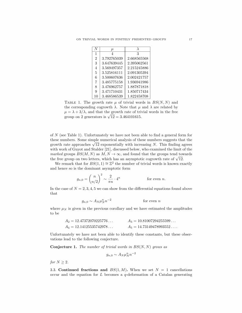
N µ λ1 4 32 3.792765039 2.6685655683 3.647639445 2.3950625614 3.569497357 2.2152458865 3.525816111 2.0913053946 3.500607636 2.0024217577 3.485775158 1.9369419868 3.476962757 1.8878718189 3.471710431 1.85071743410 3.468586539 1.822458708

Table 1. The growth rate µ of trivial words in BS(N,N) andthe corresponding cogrowth λ. Note that µ and λ are related byµ = λ+ 3/λ, and that the growth rate of trivial words in the free

group on 2 generators is√

12 = 3.464101615.

of N (see Table 1). Unfortunately we have not been able to find a general form forthese numbers. Some simple numerical analysis of these numbers suggests that thegrowth rate approaches

√12 exponentially with increasing N . This finding agrees

with work of Guyot and Stalder [21], discussed below, who examined the limit of themarked groups BS(M,N) as M,N →∞, and found that the groups tend towards

the free group on two letters, which has an asymptotic cogrowth rate of√

12.We remark that for BS(1, 1) ∼= Z2 the number of trivial words is known exactly

and hence so is the dominant asymptotic form

gn,0 =

(n

n/2

)2

∼ 2

πn· 4n for even n.

In the case of N = 2, 3, 4, 5 we can show from the differential equations found abovethat

gn,0 ∼ ANµnNn−2 for even n

where µN is given in the previous corollary and we have estimated the amplitudesto be

A2 = 12.47372070225776 . . . A3 = 10.81007294255599 . . .

A4 = 12.14125535742978 . . . A5 = 14.73149478993552 . . . .

Unfortunately we have not been able to identify these constants, but these obser-vations lead to the following conjecture.

Conjecture 1. The number of trivial words in BS(N,N) grows as

gn,0 ∼ ANµnNn−2

for N ≥ 2.

3.3. Continued fractions and BS(1,M). When we set N = 1 cancellationsoccur and the equation for L becomes a q-deformation of a Catalan generating


function:

L(z; q) = 1 + z(q + q)L(z; q) + z2L(z; q)L(z; qM ) =1

1− z(q + q)− L(z; qM ),

L(z; 1) =1− 2z −

√1− 4z

2z2.

(3.10)

Setting q = 1 into the first equation reduces it to algebraic and it is readily solved togive L(z; 1) which is the generating function of the Catalan numbers. Thus L(z; q)is a q-deformation of the Catalan numbers and rearranging the first equation showsthat L(z; q) has a simple continued fraction expansion.

L(z; q) =1

1− z(q + q−1)− z2

1− z(qM + q−M )− z2

1− z(qM2 + q−M2)− · · ·

.(3.11)

Such continued fraction forms are well known and understood in Catalan objects(see [15] for example). Unfortunately the equation for K does not simplify:

K = 1 + z(q + q)K + z2L(z; qM ) · [K − ΦM,M ◦K] + z2K · [ΦM,1 ◦K] .(3.12)

Though as noted above K(z; 1) = L(z; 1) and so we expect K(z; q) to be a differentq-deformation of the Catalan numbers. For G we have made even less progressand we have not found G(z; 1), let alone G(z; q), in closed form. Because of theq-deformed nature of L(z; q) we conjecture the following

Conjecture 2. For Baumslag-Solitar groups BS(1,M) with M > 1, the generatingfunctions G(z; q) and [q0]G(z; q) are not D-finite.

Since any path that contributes to K or L must also contribute to G, it followsthat the radius of convergence of G(z; 1) is at most 1/4 — and of course cannot beany smaller. Since the groups BS(1, N) are all amenable, we know that gn,0 ∼ 4n.We have been unable to prove any more precise details of the asymptotic form,though it is not unreasonable to expect that

gn,0 ∼ A4nn−γM .(3.13)

While we have been able to generate the first 50-60 terms of the series for M ≤ 5by iterating the equations, the series are quite badly behaved and we have beenunable to produce reasonable estimates of γM .

3.4. When N 6= M . When N 6= M , we expect that the operators ΦN,M andΦM,N in the equations satisfied by G,K,L give rise to q-deformations similar tothose observed above. In light of this, we extend our previous conjecture:

Conjecture 2 (Extended from the above). For Baumslag-Solitar groups BS(N,M)the generating functions G(z; q) and [q0]G(z; q) are only D-finite when N = M .

In spite of the absence of D-finite recurrences, we can still use the equations aboveto determine the first few terms of the cogrowth series. The resulting algorithm tocompute the first n terms of the series requires time and memory that are exponen-tial in n. The coefficient of zn is a Laurent polynomial whose degree is exponentialin n and this exponential growth becomes worse as max{N/M,M/N} becomeslarger. In spite of this, iteration of these equations to obtain the cogrowth series is


HHHHHNM

1 2 3 4 5

1 4 4 4 4 42 ◦ 3.792765039 3.724? 3.701? 3.676?3 ◦ ◦ 3.647639445 3.604? 3.585?4 ◦ ◦ ◦ 3.569497357 3.538?5 ◦ ◦ ◦ ◦ 3.525816111

Table 2. Exact and estimated growth rates of trivial words forBaumslag-Solitar groups BS(N,M). The estimated growth ratesare denoted with a ? and we expect that the error lies in the lastdecimal place — due to the difficulty of obtaining estimates, theyshould be considered to be quite rough.

exponentially faster than more naive methods based on say a simple backtrackingexploration of the Cayley graph, or iteration of the corresponding adjacency matrix.

The time and memory requirements can be further improved since we are pri-marily interested in the constant term; this means that we do not need to keep highpowers of q. More precisely if we wish to compute the series to O(zn), then weonly need to retain those powers of q that will contribute to [q0zn]G(z; q). We mustcompute the coefficients of zk for k ≤ n/2 exactly, but we can “trim” subsequentcoefficients — the degree of zn/2+k needs only be that of zn/2+k.

Simple c++ code using cln6 running on a moderate desktop allowed us to generateabout the first 50 terms of [q0]G(z; q) for BS(1, 5) while over 300 terms for BS(4, 5)were obtained. The series lengths for the other (with N < M ≤ 5) ranged betweenthese extremes. We have estimated the growth rate of trivial words using differentialapproximants — see Table 2. Again like the N = 1 case, we find the series to bevery badly behaved (except when N = M) and we have only obtained quite roughestimates.

3.5. The limit as N,M → ∞. Beautiful work of Luc Guyot and Yves Stalder[21] demonstrates that in the limit as N,M → ∞ the (marked) group BS(N,M)becomes the free group on 2 generators. We note that we can observe this freegroup behaviour in the functional equations we have obtained.

In particular as N,M →∞, the operators ΦN,N ,ΦM,M ,ΦN,M and ΦM,N becomethe constant-term operators. So in this limit the equations for K and L fromProposition 3.1 become

L = 1 + z(q + q)L+ z2L · [L0 +K0]− z2K0L0,

K = 1 + z(q + q)K + z2K · [K0 + L0]− z2K0L0,(3.14)

where K0(z) = [q0]K(z; q) and L0(z) = [q0]L(z; q). Clearly K(z; q) = L(z; q) andso with a little rearranging

L(z; q) =1− z2L0(z)2

1− z(q + q)− 2z2L0(z)=

1− z2L20

1− 2z2L0

∑n≥0

(z(q + q)

1− 2z2L0

)n.(3.15)

6An open source c++ library for computations with large integers. At time of writing it isavailable from http://www.ginac.de/CLN/


Taking the constant term of both sides then gives

L0 =1− z2L2

0

1− 2z2L0

∑n≥0

(2n

n

)(z

1− 2z2L0

)2n

=1− z2L2

0

1− 2z2L0

[1− 4

(z

1− 2z2L0

)2]−1/2(3.16)

Simplifying this last expression further gives (3z2L02−L0+1)(z2L02−L0−1) = 0.The only positive term power series solution of this gives L0 and a similar exercisegives [q0]G(z; q):

L0 =1−√

1− 12z2

6z2[q0]G =

3

1 + 2√

1− 12z2(3.17)

The expression for [q0]G is the number of trivial words in the free group on 2generators.

4. Analysis of random sampling data

4.1. Preliminaries. Using our multiple Markov chain Monte Carlo algorithm wehave sampled trivial words from the following groups:

• Thompson’s group F with the following 3 presentations

〈a, b | [ab−1, a−1ba], [ab−1, a−2ba2]〉,(4.1)

〈a, b, c, d | c = a−1ba, d = a−1ca, [ab−1, c], [ab−1, d]〉,(4.2)

〈a, b, c, d, e | c = a−1ba, d = a−1ca, e = ab−1, [e, c], [e, d]〉.(4.3)

Note that the generators a, b, c, d above are often called x0, x1, x2, x3 re-spectively in Thompson’s group literature. We have use some simple Tietzetransformations (see [28] p. 89) to obtain the second and third presenta-tions from the first (standard) finite presentation of F .

• Baumslag-Solitar groups BS(N,M) with

(N,M) = (1, 1), (1, 2), (1, 3), (2, 2), (2, 3), (3, 3), (3, 5).

• The Basilica group has presentation

(4.4) G = 〈a, b, | [an, [an, bn]] and[bn, [bn, a2n]

], n a power of 2〉

and embeds in the finitely presented group [20]

(4.5) G = 〈a, t | at2 = a2,[[

[a, t−1], a], a]

= 1〉.The groups G and G are both amenable [4].

We examined two presentations of G: The first is obtained from theabove by putting b = [a, t−1], and the second by putting b = at. Simplifi-cation gives the representations

G = 〈a, b, t | [a, t−1] = b , at2

= aa , [[b, a], a] = 1〉,(4.6)

G = 〈a, b, t | at = b , bt = a2 , b−1aba−1b−1a−1ba = 1〉.(4.7)

• Other groups for which the cogrowth series is known:

K1 = 〈a, b | a2 = b3 = 1〉,K2 = 〈a, b | a3 = b3 = 1〉,K3 = 〈a, b, c | a2 = b2 = c2 = 1〉.(4.8)


The exact solutions for BS(1, 1) ∼= Z2, BS(2, 2) and BS(3, 3) are described above,and for the other Baumslag-Solitar groups we have computed series expansions.For the last three groups, the cogrowth series were found by Kouksov [26] and are(respectively)

C(t) =(1 + t)

([0,−1, 1,−8, 3,−9] + (2− t+ 6t2)

√[1,−2, 1,−6,−8,−18, 9,−54, 81]

)2(1− 3t)(1 + 3t2)(1 + 3t+ 3t2)(1− t+ 3t2)

C(t) =(1 + t)(−t+

√1− 2t− t2 − 6t3 + 9t4)

(1− 3t)(1 + 2t+ 3t2)

C(t) =−1− 5t2 + 3

√1− 22t2 + 25t4

2(1− 25t2)

(4.9)

where [c0, c1, . . . , cn] = c0 + c1t+ · · ·+ cntn.

In each case we have obtained estimates of the mean length of freely reducedwords as a function of β. More precisely, for each group we estimated

E(nk)(β) =

∑ω |w|k(|w|+ 1)1+αβ|w|∑ω(|w|+ 1)1+αβ|w|

(4.10)

for k = ±1,±2 and a range of different α values and where the sum is over allnon-empty freely reduced trivial words. These expectations are dependent on α,but one can use Equation (2.22) to form α-independent estimates of the canonicalexpectations. Given a knowledge of the cogrowth series we can quickly computethese same means to any desired precision, since we can also write

E(nk)(β) =∑n≥0

nk(n+ 1)1+αpnβn

(n+ 1)1+αpnβn(4.11)

where pn is the number of freely reduced words of length n. Note that as α is in-creased, the samples are biased towards longer words. This expression is convergentfor β below the reciprocal of the cogrowth (being the critical point of the associatedgenerating function) and divergent above it. The convergence at the critical pointdepends on the precise details of the asymptotics of pn and will be effected by α.This then points to a simple way to test for amenability:

If the mean length of sampled words from a group on k generators is finitefor β slightly above βc = (2k − 1)−1 then the group is not amenable.

4.2. Amenable groups. We studied the groups Z2 ∼= BS(1, 1), BS(1, 2) andBS(1, 3). The cogrowth series for Z2 is known exactly, while we relied on ourseries expansions to compute statistics for the other two groups — Figure 3 showsthe plots of the mean length as a function of β.

In the case of BS(1, 1) ∼= Z2 we see excellent agreement between the numericalestimates generated by our algorithm and the mean length computed from the exactcogrowth series. ForBS(1, 2) andBS(1, 3) we see good agreement for low β betweenour numerical data and mean length computed from the exact cogrowth series.However at larger values of β it appears that the cogrowth series systematicallyunderestimates the mean length, compared to the numerical Monte Carlo data.This is, in fact, due to the modest length of the cogrowth series used to computemean lengths. For BS(1, 2) and BS(1, 3) we were only able to obtain series of


0.25 0.275 0.3 0.325

β

0

50

100

〈n〉

(a) BS(1, 1) sampled with α = 1.

0.25 0.275 0.3 0.325

β

0

20

40

〈n〉

(b) BS(1, 2) sampled with α = 1.

0.25 0.275 0.3 0.325

β

0

20

40

〈n〉

(c) BS(1, 3) sampled with α = 2.

Figure 3. Mean length of freely reduced trivial words inBaumslag-Solitar groups BS(1, 1), BS(1, 2) and BS(1, 3) at differ-ent values of β — see equation (4.10) with k = 1 and α as indicated.The sampled points are indicated with impulses, while the exactvalues are given by the black line. There is excellent agreementin the case of BS(1, 1), but a systematic error for BS(1, 2) andBS(1, 3) coming from the modest length of the exact series. Thedotted lines in these two cases indicate mean length data generatedfrom longer but approximate series.

length 60 and 56 respectively due to memory constraints. Given longer series weexpect much better agreement.

One can, for example, compute longer “approximate” cogrowth series by ignoringsmall terms. When iterating the functional equations given in Proposition 3.1 onecan form reasonable approximations by discarding coefficients gn,k which are smallcompared to nearby coefficients.7 More precisely we found that if we discard gn,kwhen 212 · gn,k <

∑k gn,k, then we obtain good approximations of the cogrowth

series. This means that only the large central coefficients are kept and far lessmemory used. This made it feasible to approximate the cogrowth series out to

7Rather than iterating the equations for G(z; q) and then transforming the result to get an

approximate cogrowth series, we found that our approximation procedure worked best if we iter-ated the slightly more complicated equations for the cogrowth series directly — see text following

Proposition 3.1 for a description of those equations.


around 200 or 300 terms. Of course, the results of these approximation should onlybe considered a rough guide as we have not bounded the size of any resulting errors.That being said, we see very good agreement between these approximations andour numerical data.

As noted above, we had great difficulty fitting the series data for BS(1, 2) andBS(1, 3). We believe that this is due to the presence of complicated confluentcorrections (likely logarithmic terms). Similar corrections also appear to be presentin the mean-length data for these groups and we were unable to find convincing orconsistent fits to any reasonable functional forms. We did, however, find that theestimated standard error was a good indicator of the location of the singularity:The standard error will diverge as β approaches the critical value of 1/3. We foundthat linear or quadratic least squares fits of the reciprocal of the error, and findingtheir x-intercept gave consistent, though perhaps slightly low, estimates of thelocation of the singularity. See Figure 4. The extrapolations give estimates β =0.330 ± 0.0002, 0.332 ± 0.002 and β = 0.332 ± 0.002 for BS(1, 1), BS(1, 2) andBS(1, 3) respectively.

Error bars above were determined by estimating a systematic error in our data.The systematic error was determined by considering the spread of estimates dueto our choices of the parameter α, the number of data points in the fits, and thechosen functional form for extrapolating the data. We believe that our results givea good indication of quality of the estimates, though we are reluctant to expressthem as firm confidence intervals. The same general approach to the data for theother groups are followed below.

The HNN-extension of the Basilica group were similarly submitted to MonteCarlo simulation by using the representations (4.6) and (4.7). The canonical ex-pected length of the words, 〈|w|〉, were computed using the ratio estimator (2.22),and turned out to be remarkably insensitive to the parameter β (see Figure 5). Thismade this group more challenging from a numerical perspective than the Baumslag-Solitar groups discussed above. Putting α = 5 finally gave acceptable results: Thesample average length show a divergence close to the critical point (since this groupis known to be amenable, this is expected to be at β = 0.2). As in the case of theBaumslag-Solitar groups, the critical value of β was determined by extrapolatingthe reciprocal of the error. Extrapolating the curve corresponding to representa-tion (4.6) gave βc = 0.217 and for representation (4.7), βc = 0.204. Taking theaverage and using the absolute difference as a confidence interval gives the estimateβc = 0.21± 0.01 to two digits accuracy.

4.3. Non-amenable groups. The groups BS(N,M) with (N,M) = (2, 2), (2, 3),(3, 3), (3, 5) and the groups K1,K2,K3 contain a non-abelian free subgroup and soare non-amenable. In the case of the groups K1 and K2 the free subgroups areF ((ab), (ab−1)), and for K3 the free subgroup is F ((ab), (ac)).

As noted above, the exact cogrowth series is known exactly for Kouksov’s ex-amples and BS(2, 2), BS(3, 3), so we were able to compute the mean length curvesexactly — see Figures 6 and 8. As above, we have estimated the location of thedominant singularities for all of these groups — see Figures 7 and 9.

Unfortunately we have been unable to solve BS(2, 3) and BS(3, 5), but we usedthe recurrences of the previous section to compute the first 100 and 120 terms (re-spectively) of their cogrowth series. And as was the case for BS(1, 2) and BS(1, 3)we also computed an approximation of the cogrowth series using the same method


0.31 0.32 0.33

β

0

200

400err−

1

(a) BS(1, 1) sampled withα = 0, 1, 2, 3.

0.31 0.32 0.33

β

0

500

1000

err−

1

(b) BS(1, 2) sampled withα = 0, 1, 2, 3.

0.31 0.32 0.33 0.34

β

0

500

1000

1500

err−

1

(c) BS(1, 3) sampled with

α = 0, 1, 2, 3.

Figure 4. Plots of the reciprocal of estimated standard error inthe mean length vs beta for α = 0, 1, 2, 3 anti-clockwise from thetop. We expect that as β approaches its critical value, that thestandard error will diverge. We see that if we extrapolate thecurves then they cross the x-axis at β = 0.330±0.002, 0.332±0.002and β = 0.332±0.002 respectively — thus these extrapolations givegood estimates of the critical value of β.

described above. These are plotted against our Monte Carlo data in Figures 10and 11.

In all cases we see strong agreement between our numerical estimates and themean length curves computed from series or exact expressions. As was the casewith the amenable groups above, fitting the reciprocal of the estimated standarderror gives quite acceptable estimates of the location of the dominant singularitiesand so the cogrowth.

4.4. Thompson’s group. Finally we come to Thompson’s group for which we ex-amine three different presentations as described above. Repeating the same analy-sis we used on the previous groups we see no evidence of a singularity in the meanlength at the amenable values of β — see Figures 12 and 13. Indeed our estimates


0.05 0.1 0.15 0.2

β

0

2.5

5

7.5〈n〉

(a) Mean length with α = 5.

0.05 0.1 0.15 0.2

β

0

10000

20000

err−

1

(b) err−1 with α = 5.

Figure 5. Numerical data on the HNN-extension of the Basilicagroup. Data points indicated by � corresponds to the representa-tion in equation (4.6) and by × to the representation in equation(4.7). In both simulations α = 5. On the left is a plot of thecanonical expected length 〈n〉. These expected lengths are onlyweakly dependent on β. On the right is the reciprocal error bar onour data. This demonstrates that the error diverges as β ↗ 0.20,consistent with the fact that these this group is amenable.

of the location of the dominant singularities are

βc = 0.395± 0.005, 0.172± 0.002 and 0.134± 0.004 respectively.(4.12)

These give cogrowths of 2.53± 0.03, 5.81± 0.07 and 7.4± 0.2, all of which are wellbelow the amenable values of 3,7 and 9. We take this to be very strong evidencethat Thompson’s group F is not amenable.

5. Conclusions

We have introduced a Markov chain on freely reduced trivial words of any givenfinitely presented group. The transitions along the chain are defined in terms ofconjugations by generators and insertions of relations. These moves are irreducibleand satisfy a detailed balance condition; the limiting distribution of the chain istherefore a stretched Boltzmann distribution over trivial words.

In order to validate the algorithm we have implemented it for a range of finitelypresented groups for which the cogrowth series is known exactly. We have alsoadded to this set of groups by finding recurrences for the cogrowth series of allBaumslag-Solitar groups. Unfortunately, these recurrences do not have simpleclosed-form solutions, but can be iterated to obtain far longer series than can befound using brute-force methods. In the case of BS(N,N), the recurrences simplifysignificantly and we are able to compute the cogrowth exactly. For N = 1, . . . , 10we have found differential equations satisfied by the cogrowth series which can beused to generate the cogrowth series in polynomial time.

We see excellent agreement between our mean-length estimates and those com-puted exactly for several groups. As a further check on our simulations, two of theauthors independently coded the algorithm and compared the results. We can useour data to estimate the location of the singularity in the generating function of


0.3 0.32 0.34

β

0

50

100〈n〉

(a) 〈a, b|a2, b3〉 sampled with α = 0.

0.3 0.32 0.34 0.36

β

0

50

100

〈n〉

(b) 〈a, b|a3, b3〉 sampled with α = 0.

0.15 0.2

β

0

50

100

〈n〉

(c) 〈a, b, c|a2, b2, c2〉 sampled

with α = 1.

Figure 6. Mean length of freely reduced trivial words of the in-dicated groups. The sampled points are indicated with impulses,while the exact values are given by the black line. We have usedvertical lines to indicate β = 1/3, 1/3, 1/5 (respectively) and also thereciprocal of the cogrowth where the statistic will diverge — being0.3418821478, 0.3664068598 and 0.2192752634 respectively. Thereis excellent agreement between the numerical and exact results,except possibly at the very highest β values.

freely reduced trivial words. The location of this singularity is the reciprocal ofthe cogrowth and so turns out to be an excellent way to predict the amenability ofgroups. To test this, we used our algorithm on a range of different amenable andnon-amenable groups. In each case we found that our numerical estimate of thecogrowth was completely consistent with the known properties of the groups. Inparticular, where cogrowth is known exactly, our numerics agreed. For each non-amenable group, the numerical “signal” was robust — no evidence of a singularitywas seen at the amenable value.

Most importantly, we see absolutely no evidence that the mean length of Thomp-son’s group is divergent close to the amenable value; i.e. for 2,4 and 5 generatorpresentations we see no evidence of a singularity at β = 1/3, 1/7 or 1/9 (respectively).Indeed, in each case, the mean length appears to be very smooth for β-values somereasonable distance above these points. Varying α or examining other statistics


0.32 0.33 0.34

β

0

250

500err−

1

(a) 〈a, b|a2, b3〉 sampled withα = 0, 1, 2, 3.

0.34 0.35 0.36 0.37

β

0

500

1000

err−

1

(b) 〈a, b|a3, b3〉 sampled withα = 0, 1, 2, 3.

0.18 0.2 0.22

β

0

250

500

err−

1

(c) 〈a, b, c|a2, b2, c2〉 sampled

with α = 0, 1, 2, 3.

Figure 7. The reciprocal of the estimated standard error vs β forthe indicated groups with α = 0, 1, 2, 3 (clockwise from top in eachcase). We see that the extrapolations of the curves intersect thex-axis very close, but slightly short, of the indicated critical valuesof β — 0.3418821478, 0.3664068598 and 0.2192752634 respectively.Hence these give good, but slightly low, estimates of the location ofthe singularities β = 0.340±0.002, 0.365±0.002 and 0.219±0.001.

does not result in any substantial change with the result that values of β consistentwith amenability are excluded from our estimated error bars. Overall, our numeri-cal data lead us to the conclusion that Thompson’s group F is not amenable withhigh probability.

To further test this hypothesis we also examined a generalisation of Thompson’sgroup, namely F (3) (see [7]). We used our algorithm to compute the mean lengthof freely reduced words in two presentations of F (3), namely

〈a, b, c, d, e | d = ba, e = cb = ca, dc = db = da, ed = ec = eb = ea〉(5.1)

〈a, b, c | cb = ca, (ba)c = (ba)b = (ba)a, (cb)(ba) = (cb)c = (cb)b = (cb)a〉,(5.2)

where xy = y−1xy.8 Note that the first presentation can be written as 3 relationsof length 4 and 5 of length 6, while the second can be written as 1 relation of length

8As was the case above, the generators a, b, c, d, e are more usually written x0, . . . , x5.


0.2 0.3 0.4

β

0

50

100〈n〉


0.2 0.3 0.4

β

0

50

100

150

〈n〉


Figure 8. Mean length of freely reduced trivial words inBaumslag-Solitar groups BS(2, 2) and BS(3, 3) at different valuesof β. The sampled points are indicated with impulses, while theexact values are given by the black line. We have used vertical linesto indicate β = 1/3 and also the reciprocal of the cogrowth wherethe statistic will diverge — being 0.3747331572 and 0.417525628respectively. We see excellent agreement between our numericaldata and the exact results, and our error bars are smaller than theimpulses.

0.34 0.35 0.36 0.37

β

0

500

1000

1500

err−

1

(a) BS(2, 2) sampled withα = 0, 1, 2, 3.

0.38 0.39 0.4 0.41

β

0

500

1000

1500

err−

1

(b) BS(3, 3) sampled withα = 0, 1, 2, 3.

Figure 9. The reciprocal of the estimated standard error of themean length as a function of β for BS(2, 2) and BS(3, 3). Inboth plots we show 4 curves corresponding to simulations at α =0, 1, 2, 3 (anti-clockwise from top) and denote the singular values —0.3747331572 and 0.417525628 respectively — with vertical lines.Extrapolating the curves give estimates of βc = 0.372± 0.002 and0.416± 0.001 respectively.

6, 4 of length 10 and 1 of length 14. As was the case for Thompson’s group F wefound no evidence of singularities at β = 1/9, 1/5 respectively.


0.25 0.3 0.35 0.4

β

20

40

60〈n〉


0.25 0.3 0.35 0.4

β

20

40

60

〈n〉


Figure 10. The mean length of trivial words in BS(2, 3) andBS(3, 5) at different values of β. We see very good for low andmoderate values of β and by systematic errors for larger β. Again,this error arises from from the modest length of the exact series.The dotted curves in these two cases indicate mean length datagenerated from longer but approximate series, while the dottedvertical lines indicate the estimated critical value of β from series.

0.36 0.37 0.38 0.39

β

0

500

1000

1500

err−

1

(a) BS(2, 3) sampled with

α = 0, 1, 2, 3.

0.41 0.42 0.43 0.44

β

0

500

1000

err−

1

(b) BS(3, 5) sampled with

α = 0, 1, 2, 3.

Figure 11. The reciprocal of the estimated standard error of themean length as a function of β for BS(2, 3) and BS(3, 5). In bothplots we show 4 curves corresponding to simulations at α = 0, 1, 2, 3(anti-clockwise from top). Extrapolating these curves we estimateβc = 0.388 ± 0.02 and 0.444 ± 0.002 for BS(2, 3) and BS(3, 5)respectively. These are quite close to the estimates from series of0.393 and 0.443 (indicated with vertical lines).

As an additional note, we have applied our methods to a finitely generated,but not finitely presented group — namely the lamplighter group. In this case thealgorithm has to be modified slightly. One can no longer choose relations uniformlyat random, but instead we choose them from distribution P (R) over the relations.As noted in section 2, this distribution must be positive and and one must have


0.25 0.3 0.35 0.4

β

0

20

40

60

〈n〉

(a) Standard presentation

(4.1) for F sampled withα = 2

0.1 0.15

β

0

20

40

60

〈n〉

(b) Presentation (4.2) for F

sampled with α = 2

0.08 0.1 0.12 0.14

β

0

20

40

60

〈n〉

(c) Presentation (4.3) for F

sampled with α = 1

Figure 12. Mean length of freely reduced trivial words in Thomp-son’s group F at different values of β. The solid blue lines indicatethe reciprocal of the cogrowth of amenable groups with k genera-tors βc = 1/2k−1. The dashed blue lines indicate the approximatelocation of the vertical asymptote. In each case, we see that themean length of trivial words is finite for β-values at and slightlyabove βc. This is strong evidence that Thompson’s group is notamenable.

P (R) = P (R−1). With these conditions the algorithm remains ergodic on thespace of trivial words and the stationary distribution is still a stretched Boltzmanndistribution. This leaves a great deal of freedom in choosing P , and our experimentsindicated that our results were quite independent of P and are consistent with theamenability of the group.

Acknowledgements

The authors thank Manuel Kauers for assistance with establishing the differ-ential equations described in Section 3.2. Similarly we thank Tony Guttmann fordiscussions on the analysis of series data. Finally we would like to thank SeanCleary and Stu Whittington for many fruitful discussions.


0.36 0.38 0.4

β

0

500

1000

1500err−

1

(a) Standard presentation(4.1) for F sampled with

α = 0, 1, 2, 3.

0.15 0.16 0.17

β

0

500

1000

1500

err−

1

(b) Presentation (4.2) for Fsampled with α = 0, 1, 2, 3.

0.11 0.12 0.13 0.14

β

0

1000

2000

err−

1

(c) Presentation (4.3) for F

sampled with α = 0, 1, 2, 3.

Figure 13. The reciprocal of the estimated standard error ofthe mean length as a function of β for the three presentationsof Thompson’s group. In each plots we show 4 curves correspond-ing to simulations at α = 0, 1, 2, 3 (anti-clockwise from top). Ex-trapolating these curves leads to estimates of βc of 0.395 ± 0.005,0.172 ± 0.002, 0.134 ± 0.004. These are all well above the valuesof amenable groups and so we take this to be strong evidence thatThompson’s group is not amenable.

The first author is supported by the Australian Research Council (ARC), andthe second and third authors are supported by grants from the Natural Sciencesand Engineering Research Council of Canada (NSERC).

References

1. C. Aragao de Carvalho and S. Caracciolo, A new Monte Carlo approach to the critical prop-erties of self-avoiding random walks, J. Physique 44 (1983), no. 3, 323–331. MR 702248

(85a:65006)

2. C. Aragao de Carvalho, S. Caracciolo, and J. Frohlich, Polymers and gϕ4 theory in fourdimensions, Nuclear Phys. B 215 (1983), no. 2, 209–248. MR 690735 (84j:81068)

3. Goulnara N. Arzhantseva, Victor S. Guba, Martin Lustig, and Jean-Philippe Preaux, TestingCayley graph densities, Ann. Math. Blaise Pascal 15 (2008), no. 2, 233–286. MR 2473819

(2009j:20052)


4. L. Bartholdi and B. Virag, Amenability via random walks, Duke Math. J. 130 (2005), no. 1,

39–56. MR 2176547

5. R.E. Bellman, Introduction to matrix analysis, vol. 19, Society for Industrial Mathematics,1997.

6. B. Berg and D. Foerster, Random paths and random surfaces on a digital computer, Phys.

Lett. B 106 (1981), no. 4, 323–326. MR 634931 (82k:65002)7. J. Burillo, S. Cleary, and M.I. Stein, Metrics and embeddings of generalizations of Thompson’s

group f , Transactions of the American Mathematical Society 353 (2001), no. 4, 1677–1690.

8. Jose Burillo, Sean Cleary, and Bert Wiest, Computational explorations in Thompson’s groupF , Geometric group theory, Trends Math., Birkhauser, Basel, 2007, pp. 21–35. MR 2395786

(2009c:20071)

9. J. W. Cannon and W. J. Floyd, What is . . . Thompson’s group?, Notices Amer. Math. Soc.58 (2011), no. 8, 1112–1113. MR 2856142

10. J. W. Cannon, W. J. Floyd, and W. R. Parry, Introductory notes on Richard Thompson’sgroups, Enseign. Math. (2) 42 (1996), no. 3-4, 215–256. MR 1426438 (98g:20058)

11. S. Chen, M. Kauers, and M. Singer, Telescopers for rational and algebraic functions via

residues, Proceedings of ISSAC, 2012, Also preprint arXiv:1201.1954, pp. 130–137.12. Joel M. Cohen, Cogrowth and amenability of discrete groups, J. Funct. Anal. 48 (1982), no. 3,

301–309. MR 678175 (85e:43004)

13. P.G. De Gennes, Scaling concepts in polymer physics, Cornell Univ Pr, 1979.14. Murray Elder, Andrew Rechnitzer, and Thomas Wong, On the cogrowth of Thompson’s group

F , To appear in Groups, Complexity, Cryptography, 2012.

15. P. Flajolet, Combinatorial aspects of continued fractions, Discrete Mathematics 32 (1980),no. 2, 125–161.

16. P. Flajolet and R. Sedgewick, Analytic combinatorics, Cambridge Univ Pr, 2009.

17. P.J. Flory, Principles of polymer chemistry, Cornell Univ Pr, 1953.18. C.J. Geyer and E.A. Thompson, Annealing markov chain monte carlo with applications to

ancestral inference, Journal of the American Statistical Association (1995), 909–920.19. R. I. Grigorchuk, Symmetrical random walks on discrete groups, Multicomponent random sys-

tems, Adv. Probab. Related Topics, vol. 6, Dekker, New York, 1980, pp. 285–325. MR 599539

(83k:60016)

20. R.I. Grigorchuk and Zuk A., On a torsion-free weakly branch group defined by a three state

automaton, International conference on geometric and combinatorial methods in group theory

and semigroup theory, Internat. J. Algebra Comput., vol. 12, World Scientific, Singapore, 2002,pp. 223–246. MR 1902367

21. Luc Guyot and Yves Stalder, Limits of Baumslag-Solitar groups, Groups Geom. Dyn. 2 (2008),no. 3, 353–381. MR 2415304 (2009d:20058)

22. J.M. Hammersley, G.M. Torrie, and S.G. Whittington, Self-avoiding walks interacting with a

surface, Journal of Physics A: Mathematical and General 15 (1982), no. 2, 539.23. EJ Janse van Rensburg, Monte carlo methods for the self-avoiding walk, Journal of Physics

A: Mathematical and Theoretical 42 (2009), 323001.

24. M. Kauers, Guessing handbook, Tech. report, Johannes Kepler Universitat, 2009.25. Dmitri Kouksov, On rationality of the cogrowth series, Proc. Amer. Math. Soc. 126 (1998),

no. 10, 2845–2847. MR 1487319 (99a:20031)

26. , Cogrowth series of free products of finite and free groups, Glasg. Math. J. 41 (1999),no. 1, 19–31. MR 1689726 (2000g:20076)

27. L. Lipshitz, D-finite power series, Journal of Algebra 122 (1989), no. 2, 353–373.28. Roger C. Lyndon and Paul E. Schupp, Combinatorial group theory, Springer-Verlag, Berlin,

1977, Ergebnisse der Mathematik und ihrer Grenzgebiete, Band 89. MR MR0577064 (58

#28182)29. Neal Madras and Gordon Slade, The self-avoiding walk, Probability and its Applications,

Birkhauser Boston Inc., Boston, MA, 1993. MR 1197356 (94f:82002)

30. Avinoam Mann, How groups grow, London Mathematical Society Lecture Note Series, vol.395, Cambridge University Press, Cambridge, 2012. MR 2894945

31. N. Metropolis, A.W. Rosenbluth, M.N. Rosenbluth, A.H. Teller, E. Teller, et al., Equation of

state calculations by fast computing machines, Journal of Chemical Physics 21 (1953), no. 6,1087.

32. R.P. Stanley, Differentiably finite power series, European J. Combin 1 (1980), no. 2, 175–188.


33. M.C. Tesi, E.J. Janse van Rensburg, E. Orlandini, and S.G. Whittington, Monte carlo study

of the interacting self-avoiding walk model in three dimensions, Journal of Statistical Physics

82 (1996), no. 1, 155–181.34. Stan Wagon, The Banach-Tarski paradox, Cambridge University Press, Cambridge, 1993,

With a foreword by Jan Mycielski, Corrected reprint of the 1985 original. MR 1251963

(94g:04005)

School of Mathematical & Physical Sciences, The University of Newcastle, Callaghan,New South Wales, Australia

E-mail address: [email protected]

Department of Mathematics, University of British Columbia, Vancouver, British

Columbia, Canada


York University, Toronto, Ontario, Canada


Department of Mathematics, University of British Columbia, Vancouver, British

Columbia, CanadaE-mail address: [email protected]

Documents

ON TRIVIAL WORDS IN FINITELY PRESENTED GROUPSandrewr/pubs/trivial_words.pdfIn this article we consider the function that counts the number of trivial words in a nitely presented group,