On the Total Variation of High-Order Semi-Discrete Central

DOI: 10.1007/s10915-005-9046-8Journal of Scientific Computing, Vol. 27, Nos. 1–3, June 2006 (© 2006)

On the Total Variation of High-Order Semi-DiscreteCentral Schemes for Conservation Laws

Steve Bryson1 and Doron Levy2

Received October 14, 2004; accepted (in revised form) March 16, 2005; Published online March 13, 2006

We discuss a new fifth-order, semi-discrete, central-upwind scheme for solvingone-dimensional systems of conservation laws. This scheme combines a fifth-order WENO reconstruction, a semi-discrete central-upwind numerical flux,and a strong stability preserving Runge–Kutta method. We test our methodwith various examples, and give particular attention to the evolution of thetotal variation of the approximations.

KEY WORDS: High-order; central schemes; conservation laws; total variation.

AMS(MOS) SUBJECT CLASSIFICATION. 65M06.

1. INTRODUCTION

In this paper we present a fifth-order, essentially non-oscillatorycentral-upwind scheme that is designed to solve systems of conservationlaws of the form

qt +f (q)x =0. (1.1)

Here q ∈Rp is a p-dimensional solution vector and f is a p-dimensional flux

function. The solution of (1.1) may become singular in finite time, which inturn requires a careful study when dealing with numerical approximations.

One approach to approximating solutions of (1.1) is to use high-order,non-oscillatory central methods, which were introduced in [15]. Centralmethods avoid approximating the solution of (1.1) at singularities of the

1 NASA Advanced Supercomputing Division, NASA Ames Research Center, Moffett Field,CA 94035-1000, USA. E-mail: [email protected]

2 Department of Mathematics, Stanford University, Stanford, CA 94305-2125, USA. E-mail:[email protected]

163

0885-7474/06/0600-0163/0 © 2006 Springer Science+Business Media, Inc.

164 Bryson and Levy

solution, and so do not require solving Riemann problems. The result-ing simplicity makes central schemes well-suited for systems and multipledimensions. Central-upwind schemes, introduced in [7] and refined in [5],are semi-discrete variants of central methods which have improved effi-ciency and less dissipation than fully-discrete central methods. Our workuses the numerical flux of [5], which we refer to as the KNP flux.

In this work we combine the KNP flux with the fifth-order weightedessentially non-oscillatory (WENO) reconstruction of [3], and the five-stage fourth-order strong stability preserving (SSP) Runge–Kutta methodof [19], which is based on [1]. This is the first time these particular ingre-dients are combined into one scheme.

Fourth-order fully-discrete central schemes based on WENO recon-structions were presented in [10, 13]. The total variation behavior ofthese methods was examined in [12], where numerical experiments sug-gest that though the WENO-based methods are not total variation dimin-ishing (TVD), they are total variation bounded. Fifth- and ninth-orderfully-discrete central schemes are discussed in [16]. Third-order extensionsof the KNP scheme can be found in [4, 6].

In this paper, we investigate the evolution in time of the total varia-tion (TV) of our scheme. The TV is defined for a discrete solution uj asTV (u) :=∑j

∣∣uj+1 −uj

∣∣. In the case of systems TV is defined as the sum

of the TV over the components. A scheme is called TV bounded (TVB)in 0 � t � T if TV (u) � K for fixed K > 0 which depends only on initialconditions, and ∀n and ∀�t � �t0 such that n�t � T and �t0 is providedby the stability requirement. In the scalar case, if a scheme is TVB thenthere exists a convergent subsequence in L1

loc to a weak solution of (1.1),which turns into strong convergence if an additional entropy condition issatisfied (see [9]). Our numerical experiments suggest that our method isTVB, providing evidence of the convergence of the method.

The structure of this paper is as follows: in Sec. 2 we present ourfifth-order central-upwind scheme, summarizing the derivation of the KNPflux in Sec. 2.1. The WENO reconstruction is summarized in Sec. 2.2. Sec-tion 3 presents the results of a number of numerical tests of our method.We test both the accuracy and the evolution of the total variation of theresulting approximations.

2. THE NUMERICAL SCHEME

We briefly summarize the components we use to construct our fifth-order central-upwind scheme: the numerical flux from [5], and the recon-struction from [3].

High-Order Semi-Discrete Central Schemes for Conservation Laws 165

2.1. The KNP Flux

Throughout this section, we assume a one-dimensional grid {xj } withconstant spacing �x. We define x

j± 12

:= xj ± 12�x and the cell Ij =

[xj− 1

2, x

j+ 12

]. For any function f (x) we use the notation fj :=f

(xj

). The

cell average of q in the cell Ij is given by q̄j := 1�x

∫ xj+ 1

2xj− 1

2q (x) dx.

We assume that the cell-averages q̄nj are known at time tn. The first

step in the derivation of the approximate solution is to generate a piece-wise-polynomial reconstruction from these cell-averages. Such a globalreconstruction is defined as q̃ (x) =∑

j q̃j (x)χIj (x) , where χIj (x) is thecharacteristic function of Ij , and q̃j (x) are polynomials of a suitabledegree.

In each cell Ij the reconstruction q̃j (x) should be conservative, i.e.1

�x

∫ xj+ 1

2xj− 1

2q̃j (x) dx = q̄j , formally sth-order accurate, (so q̃j (x) = q (x) +

O (�xs) for sufficiently smooth q and x ∈ Ij ), and non-oscillatory. Givensuch a reconstruction, we denote the point-values of q̃ at the interfaces ofthe cell Ij by q+

j+ 12

:= q̃j+1

(xj+ 1

2

)and q−

j+ 12

:= q̃j

(xj+ 1

2

).

The left- and right-sided local speeds of propagation of informationfrom the discontinuities at the cell interfaces, a±

j+ 12, are estimated by

a+j+ 1

2= max

u∈C

(

q−j+ 1

2,q+

j+ 12

)

(

λN

(∂f

∂q(u)

)

,0)

,

a−j+ 1

2=

∣∣∣∣∣∣∣∣∣

min

u∈C

(

q−j+ 1

2,q+

j+ 12

)

(

λ1

(∂f

∂q(u)

)

,0)

∣∣∣∣∣∣∣∣∣

.

Here, λ1 < · · · < λN denote the N eigenvalues of the Jacobian of f and

C

(

q−j+ 1

2, q+

j+ 12

)

is the curve in phase space connecting q−j+ 1

2and q+

j+ 12.

These local speeds of propagation are then used to determine intervalsfor averaging that contain the Riemann fans from the cell interfaces. Anexact evolution of the reconstruction is followed by an intermediate piece-wise polynomial reconstruction and finally projected back onto the orig-inal cells, providing the cell-averages at the next time-step q̄n+1

j . Furtherdetails can be found in [5]. A semi-discrete scheme is obtained in the limit

166 Bryson and Levy

as �t →0, yielding the KNP central-upwind scheme

dq̄j

dt=−

Hj+ 1

2−H

j− 12

xj+ 1

2−x

j− 12

. (2.1)

The numerical flux in (2.1) is given by

Hj+ 1

2=

a+j+ 1

2f

(

q−j+ 1

2

)

+a−j+ 1

2f

(

q+j+ 1

2

)

a+j+ 1

2+a−

j+ 12

−a+j+ 1

2a−j+ 1

2

a+j+ 1

2+a−

j+ 12

[

q+j+ 1

2−q−

j+ 12

]

.

The accuracy of this scheme is determined by the accuracy of the recon-structions and the ODE solver.

It is straightforward to generalize this scheme to higher dimensions,using dimension-by-dimension reconstructions. Care must be taken, how-ever, to use higher-order quadratures in the derivation of the KNP flux inhigher dimensions to maintain accuracy. See [6] for a third-order example.

2.2. The Fifth-Order WENO Reconstruction

Weighted, essentially non-oscillatory (WENO) reconstructions [3, 14]are based on the essentially non-oscillatory (ENO) reconstructions of [2,17]. ENO schemes choose the stencil that provide the least oscillatoryreconstruction. WENO schemes weight all stencils so that accuracy isgained in smooth regions while trying to avoid crossing discontinuities.

We use the fifth-order WENO reconstruction of the point-value qj+ 1

2given in [3]. We begin with the three quadratic reconstructions on three-point stencils

qk

j+ 12=

2∑

r=0

akr q̄j+k+r−2, (2.2)

where k ranges from 0 to 2 and the coefficients akr , given in Table I, are

defined so that (2.2) approximates q(xj+ 1

2

)with third-order accuracy. The

WENO reconstruction is then defined as the convex combination

qj+ 1

2=

2∑

k=0

wkjq

k

j+ 12, wk

j :=αk

j∑2

k=0 αkj

, αkj := Ck

(ε +Sk

j

)2. (2.3)


Table I. Coefficients akr for

the Quadratic Reconstructions(2.2)

k r =0 r =1 r =2

0 1/3 −7/6 11/61 −1/6 5/6 1/32 1/3 5/6 −1/6

The constants Ck = {1/10,6/10,3/10} are defined so that∑2

k=0 Ckqk

j+ 12

approximates q(xj+ 1

2

)with fifth-order accuracy. Sk

j is a smoothness mea-

sure which is large when qk

j+ 12

has large variation. Skj approximates the

L2loc-norm of the first two derivatives of q, and is given by

S0j = 13

12

(q̄j−2 −2q̄j−1 + q̄j

)2 + 14

(q̄j−2 −4q̄j−1 +3q̄j

)2,

S1j = 13

12

(q̄j−1 −2q̄j + q̄j+1

)2 + 14

(q̄j−1 − q̄j+1

)2, (2.4)

S2j = 13

12

(q̄j −2q̄j+1 + q̄j+2

)2 + 14

(3q̄j −4q̄j+1 + q̄j+2

)2.

Following [3] we take ε =10−6. The reconstruction of qj− 1

2on the stencil

centered at xj is obtained by symmetry. For more details consult [3].

3. NUMERICAL EXAMPLES

We test our method on various examples, measuring both the accuracyof the approximation and the evolution of the TV over time. To integrate(2.1) forward in time, we use an optimal, strong stability preserving fourth-order accurate five-stage Runge–Kutta solver from [19]. We also ran ourexamples with the standard Runge–Kutta method and observed no signifi-cant change in the results. We use the CFL condition �t = 0.45 minj

�x

|λj | ,where here λj denote the eigenvalues of the Jacobian of f evaluated at xj .

When an exact solution is not available, we use a high-resolution refer-ence solution computed using the second-order KNP method as presentedin [5], which is known to be TVD. Unless otherwise stated, this referencesolution uses N =5000 nodes.

We first test our method with the scalar advection problem ut +ux =0, u (x, t =0)= sin4 (πx) on the periodic domain [−1,1] at T =2. The rel-ative L1- and L∞- norms of the errors are shown in Table II. We also test

168 Bryson and Levy

Table II. Relative L1 and L∞ Errors for the Advection Equation and theBurgers Equation

Relative L1-error L1-order Relative L∞-error L∞-order

N Linear advection of sin4 (πx), T =2100 8.68×10−4 – 1.14×10−3 –200 2.55×10−5 5.09 4.18×10−5 4.77400 6.32×10−7 5.34 9.77×10−7 5.42800 1.46×10−8 5.44 1.49×10−8 6.03

Burgers equation before the shock, T =0.5100 1.03×10−6 – 7.51×10−6 –200 3.87×10−8 4.74 2.89×10−7 4.70400 1.15×10−9 5.08 8.12×10−9 5.15800 8.87×10−11 3.69 3.31×10−10 4.61

Burgers equation after the shock, T =2.5100 3.34×10−3 – 1.42×10−1 –200 1.99×10−3 0.75 2.12×10−1 −0.57400 8.72×10−4 1.19 1.65×10−1 0.36800 4.38×10−4 0.99 1.63×10−1 0.01

accuracy with the Burgers equation ut +(

u2

2

)

x=0, u (x, t =0)=3+ sin (x)

on the periodic domain [0,2π ] at T = 0.5, before shock formation, andat T = 2.5 after shock formation. The results are also shown in Table II.Figure 1 shows the result at T =2.5, as well as the change in the TV overtime for various resolutions. For this example the exact TV equals to 4before the singularity formation at T =1.

Our next example is Burgers equation on the same domain with ini-tial data u (x, t =0) = 2 − sin (x) + sin (2x). This example develops twoshocks which eventually merge. Figure 2 shows the solution at T = 1.2 aswell as the change in the TV over time for various resolutions.

Turning to systems, we consider the Euler equations⎛

⎝ρ

ρu

E

⎞

⎠

t

+⎛

⎝ρu

ρu2 +p

(E +p)u

⎞

⎠

x

=0 (3.1)

with equation of state p = (γ −1) (E − 12ρu2) and γ = 1.4. We first apply

our method to the Lax problem [8] on the domain [0,1] with initial data

(ρ, u,E)={

(0.445,0.311,8.928) , x <0.5,

(0.5,0.0,1.4275) , x >0.5.(3.2)

The results at T =0.16 with N =100 and N =400 grid nodes is shown inFig. 3. While the shock and the contact discontinuity are well-captured at


0 1 2 3 4 5 62

2.2

2.4

2.6

2.8

3

3.2

3.4

3.6

3.8

4

u

x

Burgers equation at T=2.5, N=100

0 0.5 1 1.5 2 2.53.2

3.3

3.4

3.5

3.6

3.7

3.8

3.9

4

TV

t

Total variation for Burgers equation at T=2.5

Fig. 1. Results for the Burgers equation using the central-upwind scheme (2.1) and (2.3).Top: the solution after shock formation at T =2.5, “−”: exact solution, “◦”: approximation.Bottom: the change in the TV of the approximation for N = 100,200,400,800 nodes (fromleft to right) compared with the TV of a reference solution (the upper curve).

170 Bryson and Levy

0 1 2 3 4 5 60

0.5

1

1.5

2

2.5

3

3.5

4

u

x

2−shock Burgers problem at T=1.2, N=100

0 0.5 1 1.5 2 2.5 3 3.5 4 4.5 52

3

4

5

6

7

8

9

TV

t

Total variation for 2−shock Burgers problem at T=5

reference solutionN = 100N = 200N = 400N = 800

Fig. 2. Results for Burgers equation with initial data that develops a double shock usingthe central-upwind scheme (2.1) and (2.3). Top: the solution after shock formation at T =1.2,“−”: exact solution, “◦”: approximation. Bottom: the change in the TV of the approximationfor various resolutions compared with the TV of a reference solution.


low resolution, there are significant oscillations between the contact dis-continuity and the shock for N =100. Figure 3 also shows the TV behav-ior of the approximation, compared with a reference solution. We see thatthe TV of the approximate solutions are initially greater than that of thereference solution, but converges to the TV of the reference solution overtime, with a faster rate of convergence for finer meshes. It is interesting,however, that the over-shoot of the TV at early times does not seem todepend on the mesh resolution. We observe similar behavior for the Sodproblem [18].

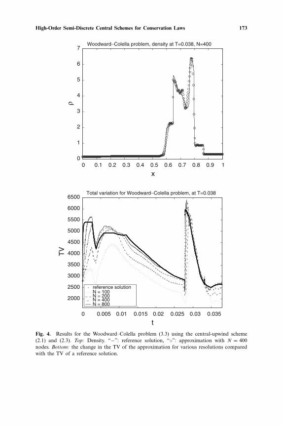
We next apply our method to the reflected blast problem of Woodwardand Colella [20], on the domain [0,1] with reflecting boundary conditionsand initial data

(ρ, u,E)=⎧⎨

⎩

(1.0,0.0,2500.0), 0�x <0.1,

(1.0,0.0,0.01), 0.1�x <0.9,

(1.0,0.0,250.0), 0.9�x �1.

(3.3)

The results at T =0.038 with N =400 grid nodes are shown in Fig. 4, com-pared with a reference solution using 10,000 nodes. We see some numericaloscillations. Figure 4 also shows the TV behavior of the approximation,compared with the reference solution. We see that the TV of the approx-imate solutions converges to the TV of the reference solution for finermeshes, but do not seem to converge over time. This is not surprising sincethis example contains sharp peaks that will not be resolved for coarsemeshes.

For our final example we apply our method to the problem of a machthree wave interacting with an acoustic shock on the domain [0,1] (see[17]). The initial conditions for this problem are

(ρ, u,p)={

(3.857143,2.629369,10.3333), x �0.1,

(1+0.2 sin (50x),0,1), x >0.1.(3.4)

The results are shown in Fig. 5, compared with a reference solution using20,000 nodes. We see the high resolution of our method and indicationsthat the TV of our approximations converges to that of the reference solu-tion.

In conclusion, we would like to note that the TV approaches the TVof the reference solution in different ways for different examples. While insome cases it is monotone (such as the acoustic-shock problem) in othercases it is not (such as the Woodward–Colella problem). Our results arecharacteristic of the complex structure that one may expect to find withthe TV of solutions of systems (with the lack of any supporting theory).Trying to convert these observations into a statement on the convergenceof the scheme remains an important topic for future study.

172 Bryson and Levy

0 0.1 0.2 0.3 0.4 0.5 0.6 0.7 0.8 0.9 10.2

0.4

0.6

0.8

1

1.2

1.4

1.6ρ

x

Lax problem density at T=0.16, N=100

0 0.02 0.04 0.06 0.08 0.1 0.12 0.14 0.1613

13.5

14

14.5

15

15.5

16

16.5

17

TV

t

Total variation for Lax problem at T=0.16


Fig. 3. Results for the Lax problem (3.2) using the central-upwind scheme (2.1) and (2.3).Top: Density. “−”: reference solution, “◦”: approximation with N =100 nodes, “+”: approx-imation with N =400 nodes. Bottom: the change in the TV of the approximation for variousresolutions compared with the TV of a reference solution.


0 0.1 0.2 0.3 0.4 0.5 0.6 0.7 0.8 0.9 10

1

2

3

4

5

6

7

ρ

x

Woodward−Colella problem, density at T=0.038, N=400

0 0.005 0.01 0.015 0.02 0.025 0.03 0.035

2000

2500

3000

3500

4000

4500

5000

5500

6000

6500

TV

t

Total variation for Woodward−Colella problem, at T=0.038


Fig. 4. Results for the Woodward–Colella problem (3.3) using the central-upwind scheme(2.1) and (2.3). Top: Density. “−”: reference solution, “◦”: approximation with N = 400nodes. Bottom: the change in the TV of the approximation for various resolutions comparedwith the TV of a reference solution.

174 Bryson and Levy

0 0.1 0.2 0.3 0.4 0.5 0.6 0.7 0.8 0.9 10.5

1

1.5

2

2.5

3

3.5

4

4.5

5

ρ

x

Acoustic problem density at T=0.18, N=400

0 0.02 0.04 0.06 0.08 0.1 0.12 0.14 0.16 0.1840

60

80

100

120

140

160

180

TV

t

Total variation for acoustic problem at T=5


Fig. 5. Results for the acoustic-shock problem (3.4), showing the approximation of thedensity field at T = 0.18 using N = 400 nodes. Top: Approximate solution. “−”: referencesolution, “◦”: approximation. Bottom: the change in the TV of the approximation for vari-ous resolutions compared with the TV of a reference solution.


ACKNOWLEDGEMENTS

The work of D. Levy was supported in part by the National ScienceFoundation under Career Grant No. DMS-0133511.

REFERENCES

1. Gottlieb, S., Shu, C.-W., and Tadmor, E. (2001). Strong stability-preserving high ordertime discretization methods. SIAM Rev. 43, 89–112.

2. Harten, A., Engquist, B., Osher, S., and Chakravarthy, S. (1987). Uniformly high orderaccurate essentially non-oscillatory schemes III. J. Comp. Phys. 71, 231–303.

3. Jiang, G.-S., and Shu, C.-W. (1996). Efficient implementation of weighted ENO schemes.J. Comp. Phys. 126, 202–228.

4. Kurganov, K., and Levy, D. (2000). A Third-order semi-discrete central scheme for con-servation laws and convection-diffusion equations. SIAM J. Sci. Comp. 22, 1461–1488.

5. Kurganov, K., Noelle, S., and Petrova, G. (2001). Semi-discrete central-upwind schemesfor hyperbolic conservation laws and Hamilton-Jacobi equations. SIAM J. Sci. Comp. 23,707–740.

6. Kurganov, K., and Petrova, G. (2001). A Third-order semi-discrete genuinely multidi-mensional central scheme for hyperbolic conservation laws and related problems. Numer.Math. 88, 683–729.

7. Kurganov, A., and Tadmor, E. (2000). New high-resolution central schemes for nonlinearconservation laws and convection-diffusion equations. J. Comp. Phys. 160, 241–282.

8. Lax, P. D. (1954). Weak solutions of nonlinear hyperbolic equations and their numericalcomputation. Comm. Pure Appl. Math. 7, 159–193.

9. LeVeque, R. J. (1992). Numerical Methods for Conservation Laws, Lectures in Mathemat-ics, Birkhuser, Basel.

10. Levy, D., Puppo, G., and Russo, G. (1999). Central WENO schemes for hyperbolicsystems of conservation laws. Math. Model. Numer. Anal. 33, 547–571.

11. Levy, D., Puppo, G., and Russo, G. (2000). Compact central WENO schemes for multi-dimensional conservation laws. SIAM J. Sci. Comp. 22, 656–672.

12. Levy, D., Puppo, G., and Russo, G. (2000). On the behavior of the total variation inCWENO methods for conservation laws. Appl. Num. Math. 33, 415–421.

13. Levy, D., Puppo, G., and Russo, G. (2002). A fourth order central WENO scheme for multi-dimensional hyperbolic systems of conservation laws. SIAM J. Sci. Comp. 24, 480–506.

14. Liu, X.-D., Osher, S., and Chan, T. (1994). Weighted essentially non-oscillatory schemes.J. Comp. Phys. 115, 200–212.

15. Nessyahu, H., and Tadmor, E. (1990). Non-oscillatory central differencing for hyperbolicconservation laws. J. Comp. Phys. 87, 408–463.

16. Qiu, J., and Shu, C.-W. (2002). On the construction, comparison, and local characteristicdecomposition for high order central WENO schemes. J. Comp. Phys. 183, 187–209.

17. Shu, C.-W., and Osher, S. (1988). Efficient implementation of essentially non-oscillatoryshock-capturing schemes. J. Comp. Phys. 77, 439–471.

18. Sod, G. (1978). A survey of several finite difference methods for systems of nonlinearhyperbolic conservation laws. J. Comp. Phys. 27, 1–31.

19. Spiteri, R. J., and Ruuth, S. J. (2002). A new class of optimal high-order strong-stability-preserving time discretization methods. SIAM J. Numer. Anal. 40, 469–491.

20. Woodward, P., and Colella, P. (1984). The numerical simulation of two-dimensional fluidflow with strong shocks. J. Comp. Phys. 54, 115–173.

Documents

On the Total Variation of High-Order Semi-Discrete Central