On the sizing of a ﬂat-panel ground heat exchanger

ORIGINAL RESEARCH

On the sizing of a flat-panel ground heat exchanger

Marco Bortoloni • Michele Bottarelli

Received: 22 July 2014 / Accepted: 23 October 2014 / Published online: 12 November 2014

� The Author(s) 2014. This article is published with open access at Springerlink.com

Abstract Ground-source heat pumps are a reliable tech-

nology and may represent an efficient and cost-effective

option for space heating and cooling, when the investment

for ground heat exchangers is reasonable. New advanced

ground exchangers have been recently proposed, showing

high performances also in shallow ground; their shape has

not yet been investigated in literature. In the present study,

an analytical solution based on the line source method is

applied for sizing a novel shape. This so-called flat-panel

shape is assumed to be an equivalent slinky-coil having the

same heat transfer surface per unit of trench length. As

overall benchmarks, two other configurations of straight

pipes disposed vertically and horizontally have been sized;

all devices are supposed to work in a four lined geothermal

field. The building heating requirement has been evaluated

assuming a simplified lumped system and three different

climate zones, defined by 2,000, 2,500 and 3,000 degree

days. Then, a 2D finite-element model has been imple-

mented to solve the transient heat conduction problem in

the ground. The results of the analytical formulation and

numerical simulations have been compared in terms of

average temperature at the wall surface of the heat

exchanger. The design minimum temperature considered

by the analytical method in sizing the two straight pipe

configurations and the flat-panel is accurately reproduced

by the numerical model. Therefore, the slinky-coil equiv-

alent approach followed in the analytical method for sizing

the flat-panel seems to be a reliable and suitable

approximation.

Keywords Horizontal ground heat exchangers �Flat-panel � Analytical method � Numerical model �Sizing comparison

List of symbols

c Building overall specific heat capacity J/(kg K)

d Depth in ground m

D Julian day of the year dimensionless

DD Degree-days �C day

Fh Heating load factor dimensionless

Lh,p Specific length of the ground heat exchanger m/m3

Pm Pipe wall resistance correction factor

dimensionless

qV Heat flux for unit building volume J/m3

_Qg;hDMaximum heating power for unit building volume

in design W/m3

QfD Overall monthly heating requirement for unit

building volume in design Wh/m3

r Ratio of plenum to building volume dimensionless

Rg Ground thermal resistance (K�m2)/W

Rp Pipe thermal resistance (K�m2)/W

S Building heat transfer surface m2

Sm Trench configuration correction factor

dimensionless

S/V Building shape ratio dimensionless

Tair Outdoor air temperature �CTd Daily average temperature of the day �CTn Daily average temperature of the night �CTt Target temperature in heating mode �CT0 Initial temperature �C

Published in the Special Issue ‘‘8th AIGE Conference (Italian

Association for Energy Management)’’.

M. Bortoloni (&)

Department of Engineering, University of Ferrara,

Via Saragat 1, 44122 Ferrara, Italy

e-mail: [email protected]

M. Bottarelli

Department of Architecture, University of Ferrara,

Via Quartieri 8, 44121 Ferrara, Italy

123

Int J Energy Environ Eng (2015) 6:55–63

DOI 10.1007/s40095-014-0150-0

U Equivalent overall building thermal transmittance

W/(m2 K)

V Indoor building heated volume m3

vh Building heated volume per unit length of the

trench m3/m

q Density kg/m3

a Soil thermal diffusivity m2/s

hg;l Ground temperature in design �ChwD Average working fluid temperature in design �ChM Annual average air temperature �C

Introduction

The European policies for energy saving in buildings and

reduction of greenhouse gas emissions widely support the

spread of renewable energy sources, especially in space

heating and cooling. In this field, ground-source heat

pumps (GSHPs) have been regarded as a reliable and

profitable technology due to their high energy efficiency,

when the design is compliant with local environmental

conditions and building energy requirements [1, 2].

Ground-coupled heat pumps (GCHPs) are a subset of

GSHPs, in which the heat transfer is performed by means

of vertical and deep boreholes heat exchangers (BHEs) or

horizontal and shallow ground heat exchangers (HGHEs).

BHEs benefit from the relatively stable temperature in deep

ground, whereas HGHEs use unsteady source/sink energy

storage, related to the solar energy balance at ground sur-

face. For HGHEs, the seasonal variation of the ground

temperature may lead to unfavourable working conditions

and, consequently, to an efficiency reduction. Nevertheless,

ground thermal drifts are not expected after long-term

operation, as reported in [3–6]. Anyway, ground heat

exchangers (GHEs) are the weakest link in GCHPs, due to

the low soil thermal diffusivity. To improve the heat

exchange efficiency and reduce the cost for the shallow

horizontal installation, new arrangements for the wide-

spread slinky-coils installation and novel shapes of GHEs

have been recently proposed [5, 6].

Because the sizing of GCHPs systems needs to consider

the history of thermal loads and the ground capacity to absorb

or provide heat, the ground coupling for a heat pump must be

sized accurately [7]. Analytical approaches based on the line

source theory and cylindrical heat transfer equations are

widely used for sizing traditional GHEs installations, as

reported in [8, 9] and recently provided for also by Italian

regulations [10]. These methods are also useful to design

some types of HGHEs adopting trench configuration, such as

straight pipes and slinky-coils; an analytical procedure was

proposed in [9, 10] to quickly determine the HGHE overall

length for these configurations. There are still relatively few

numerical solutions to the ground heat transfer problem for

new GHEs shapes because of their novelty. In [11], the effect

of the depth of installation and the soil thermal conductivity

on the performance of three different heat exchangers

(straight, helical and slinky-coil) is investigated. In [4, 12]

the commercial code FEFLOW is used to simulate the

energy performance of a slinky-coil, taking into account the

energy balance at the ground surface and new spatial

arrangements, whereas in [5] FEFLOW is implemented to

make a comparison between the energy behaviour of a flat-

panel and a radiator. Despite the long computational time

required, several numerical studies have been carried out,

because their flexibility allows implementing realistic

boundary conditions, including the mass transfer to take into

account the effects of the soil moisture, as shown in [13] or

developing an energy balance equation at the ground surface

[14]. Anyway, a method for the quick and preparatory sizing

of novel shapes of GHEs is not yet available.

In the present work, the above mentioned analytical

method [10] is used for sizing a novel type of HGHE, the so-

called flat-panel (FP), recently developed by the University

of Ferrara. The implementation has been preliminary carried

out assuming the flat-panel to be a slinky-coil having the

same heat transfer surface. For completeness, two standard

configurations of straight pipe are considered as benchmarks.

Then, all sizing has been checked by means of finite element

models implemented and solved with the same boundary

conditions used in the analytical procedure.

Methodology

This study focuses on the flat-panel (FP) sizing procedure,

performed adapting the analytical method provided by [9]

and adopted in [10], and checked by means of a numerical

model. The analysis has been carried out only in heating

mode for three different climate zones (2,000, 2,500 and

3,000 DD), and a numerical verification has been also

performed for two HGHEs standard configurations with

benchmark purpose. A commercial finite elements code

(COMSOL Multiphysics�, V4.4) has been used for solving

the heat conduction problem in a 2D symmetrical domain,

adopting hourly time series as boundary conditions in order

to consider the ground surface temperature and the energy

requirement at the HGHE. Finally, the results have been

compared in terms of temperature and energy performance,

taking into account the average temperature at the HGHE

wall surface.

Domains of the test cases

The analytical method reported in [10] is useful to assess

the overall length of trench for common GHE shapes,

56 Int J Energy Environ Eng (2015) 6:55–63

123

arrangement and energy requirement but does not solve the

problem for new shapes, such as FP. So, we have consid-

ered the FP to be equivalent to a DN20 slinky-coil having

the same heat transfer surface per unit length of trench. The

fictitious coil has a diameter of 1 m, equal to the FP height,

and its heat transfer surface area is 0.197 m2 for each coil.

In order to match the heat transfer surface of the FP (2 m2/

mtrench), 10.15 coils have been considered for unit length of

trench, split on two levels as a standard configuration

reported in [10]; thus, every metre of FP is equivalent to

31.87 m of DN20 slinky-coil.

For completeness and benchmark purposes, two other

standard HGHEs configurations have been considered,

taken from those provided in [10]. Both consists of eight

DN20 pipes; in the horizontally aligned case (HT), they are

divided in two horizontally superposed layers (4 ? 4), in

the vertically aligned case (VT), they are placed vertically,

as shown in Fig. 1. All the HGHEs are placed at the same

average depth of 1.5 m, and the geothermal system is

composed of four parallel trenches with a distance of

2.74 m between the axis of the exchangers. All pipes are

supposed to be in HDPE and have a 2 mm thickness.

Our numerical analysis considers a 2D finite element

domain consisting of a cross section which comprises the

previous HGHEs placed within trenches and a wide sur-

rounding soil volume. The soil is supposed to be homog-

enous and isotropic over the entire domain, with a thermal

conductivity of 1.3 W/(m�K), a density of 1,600 kg/m3 and

a specific heat capacity of 1,200 J/(kg�K). This assumption

is commonly used in literature for the purpose of modelling

HGHEs. Even though heterogeneity of shallow soil may

affect the results, its impact can be considered negligible,

as reported in [15].

Since the overall domain is symmetric, the heat transfer

problem is solved in a half-domain to reduce calculation

time. Hence, only two trenches are considered for the four

lined geothermal system. The computational domain is

taken to be sufficiently large to have an area undisturbed by

the system operation, and it is thus 14.0 m wide and 15.0 m

deep, as shown in Fig. 2. Given that the temperature at the

outer surface of heat exchanger has been considered, the FP

is here schematized as a vertical line, while the piping as an

empty circular hollow. In both cases, the thickness of the

wall and its thermal resistance are neglected. Figure 2 also

shows the full computational mesh and some details for

each case. To reduce the computational time and the

numerical errors, the grid size is fine at the ground surface

and close to the GHEs, coarse for the remaining area far

from it. The resulting triangular mesh is composed of up to

37,000 element, whose size ranges 17 9 10-3 cm2 for fine

grids and 103 cm2 for coarse grids. The result indepen-

dence from the meshing has been checked by doubling the

number of the elements without relevant difference.

The temperature at the GHE is then measured as the

average value across its surface. Single point values for the

ground temperature are calculated, between the trenches on

the axis of symmetry at the average depth of the system

(0.0; -1.5 m) and on an undisturbed point, 10 m far from

the exchanger (14.0; -1.5 m).

Boundary conditions

According to the sinusoidal and negative exponential var-

iation of the ground temperature reported in [10] and

originally determined in [16], boundary conditions are

calculated with regard to the following equation:

hg d;Dð Þ ¼ hM � A � cos2p365

D � D0 �1

2

ffiffiffiffiffiffiffiffiffiffi

pd2

365a

r

!" #

� e�ffiffiffiffiffi

pd2

365a

p

; ð1Þ

where hg is the daily ground temperature at depth d and

Julian day D, D0 the Julian day of the lowest temperature, athe soil thermal diffusivity, hM the annual average air

FP HT VT

1.5 m

0.9 m

DN 20 0.9 m

Fig. 1 Cross-sectional view of HGHEs configurations (FP flat-panel,

HT horizontal trench, VT vertical trench)

Fig. 2 Computational domain, mesh details

Int J Energy Environ Eng (2015) 6:55–63 57

123

temperature and A the average annual amplitude of the air

temperature.

We suppose the daily average air temperature Tair to be

equal to the daily average surface ground temperature hg,

as calculated by Eq. 1 setting d to zero. Then, the tem-

perature time series on an hourly scale is obtained super-

imposing to the daily time series a sinusoidal oscillation

ranging between the daily minimum and maximum/air

temperatures (night/day) in winter and summer, taking into

account the climate zone and a time drift due to the heat

transfer phenomenon [17].

Specifically, in order to consider the three desired dif-

ferent climate zones (2,000, 2,500 and 3,000 DD) and

control the heating requirement, we operate calibrating hM

and A, using different day/night temperatures. According to

data monitored at the Department of Architecture of Ferr-

ara University, the hourly temperature at the ground sur-

face is then smoothed by a reduction factor of 0.6 with

respect to the air temperature, and a time shift of 10 h is

applied between the hourly sinusoidal variations of air and

ground temperature.

Table 1 reports the main parameters characterizing the

climate zone supposed, while Fig. 3 shows the resulting

time series for the 2,500 degree days case in winter time.

The energy requirement for indoor space heating is

defined as the amount of energy required to maintain the

target indoor temperature in heating mode during the

winter (Tt = 20 �C). For simplicity, the heating require-

ment is here related to the outdoor air temperature time

series, assuming the building as an homogenous lumped

and closed thermodynamic system, whose internal energy

variation only occurs owing to the heat transfer through its

envelope, as reported in [18].

As consequence, when the heating system is turned off,

the average indoor temperature T(t) becomes:

T tð Þ ¼ Tair tð Þ þ T0 � Tair tð Þ� �

� e�US� t�t0ð Þ

rqVc ; ð2Þ

where T0 is the indoor air temperature at time step t0.

When the heating system is turned on, the specific

energy requirement for unit of volume of the system can be

evaluated as follows:

qðtÞ ¼ rqc � Tt � T0ð Þ½ �t¼0þ US

V� Tt � Tair tð Þð Þ � Dt

� �

t � 0

;

ð3Þ

where the first term on the r.h.s. takes into account the

energy needed to reach the target temperature (Tt) from an

initial different value (T0), and the second one the energy

required to maintain it due to the heat transfer occurring

through the envelope during the time step Dt, here assumed

equal to one hour. Because a maximum heating power of

25 W/m3 has been considered in the analytical method,

when the resulting hourly energy exceeds the previous

limit, q(t) is reduced to 25 Wh/m3 and an indoor temper-

ature lower than the target temperature is calculated by

means of Eq. 3.

According to the Italian regulations, the heating season

begins on October 15th and ends on April 15th for the

cases 2,500 and 3,000 DD, while it begins on November

1st for the case with 2,000 DD. The GCHPs operation

hours are selected to represent actual working conditions.

Cases with 2,500 and 3,000 DD involve 14 h of operation

per day, from 5 am to 10 am and 4 pm to 11 pm from

Monday to Friday, 8 am to 1 pm and 4 pm to 11 pm on

weekends. The case with 2,000 DD implies 12 h of oper-

ation per day, from 6 am to 10 am and 5 pm to 11 pm from

Monday to Friday, 8 am to 12 am and 5 pm to 11 pm on

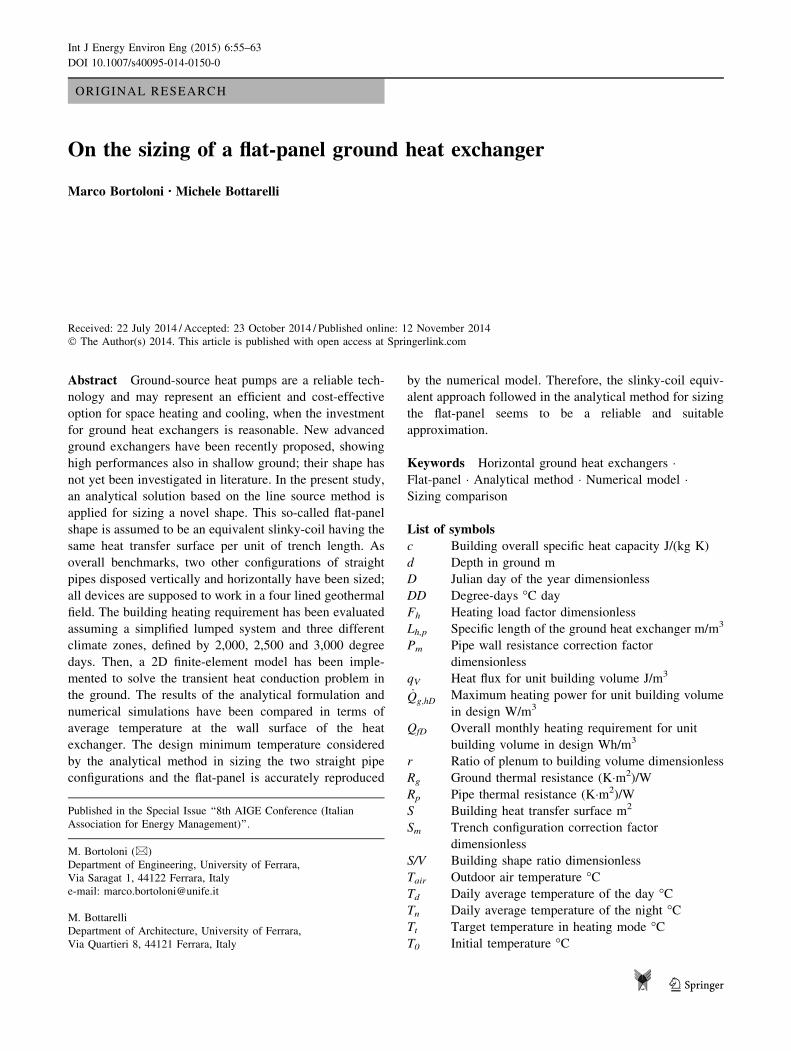
weekends. A typical week of operation for the case with

2,500 DD is shown in Fig. 4, together with the surface

ground temperature and outdoor air temperature.

Finally, the resulting time series for the operation of the

GCHPs is used to define the energy requirements at the

HGHEs in the numerical model. An equivalent time series

for each case is calculated to reproduce the same output

temperature between the two approaches, as explained in

detail in the results section.

The resulting energy requirements have been evaluated

on a monthly scale for each case. The highest energy is in

Table 1 Parameters of different climate zones

�C 2,000 DD 2,500 DD 3,000 DD

hM 16.49 13.99 10.75

A 12.50 12.00 11.25

Tmax in winter 8 6 2

Tmax in summer 34 32 28

Tmin in winter 0 -2 -3

Tmin in summer 24 20 16

-5

0

5

10

15

20

15/10 14/11 14/12 13/1 12/2 14/3 13/4

Tem

pera

ture

(°C

)

Time (day)

Tsoil, surface Tsoil, -1.5m Td Tn Tair

Fig. 3 2,500 DD, daily and hourly temperature time series for

outdoor air and soil surface in winter time


123

January for all three cases, due to the minimum value of the

air temperature time series, which occurs on 15th of Jan-

uary according to [10]. Given an overall operation time of

the GCHPs equal to 744 h in the coldest month, the specific

energy requirement is 5.095, 4.968 and 5.577 kWh/m3 for

2,000, 2,500 and 3,000 DD, respectively. The heat energy

demand in January is higher for the case 2,000 DD than for

the case 2,500 DD due to the lower daily operating time

allowed for first one. Thus, the GCHP is forced to work for

longer time at the maximum power. Consequently, it is

possible to calculate the heating load factor Fh for the three

cases considered. Given the maximum heating power and

the total operation time, Fh is 0.274, 0.267 and 0.299 for

2,000, 2,500 and 3,000 DD, respectively.

Table 2 reports the equivalent thermal properties adop-

ted for the simulated building.

Analytical method

As reported in [10], the following equation defines the

overall length of an horizontal heat exchanger:

Lh;p ¼_Qg;hD � Rp þ Rg � Pm � Sm � Fh

� �

hg;l � hwD

; ð4Þ

where _Qg;hD is the required maximum heating power, hg,l is

the minimum temperature of the soil at the HGHE average

depth, hwD is the lowest design average temperature

between inlet and outlet of the working fluid, Rp and Rg are

the thermal resistances of the pipe and the soil, Pm is a

coefficient related to the diameter of the pipes, Sm is the

correction factor related to the distance between the tren-

ches, and Fh is the heating load factor of the month with the

highest heat requirement.

The values of Rg, Pm and Sm depend on the configuration

of the heat exchanger, and are provided by tables reported

in [10]. For the FP case, these are obtained through the

equivalence to a slinky-coil described above, and then by

interpolation. According to [10], Pm is taken equal to 1,

since the diameter of the pipes is DN20, whereas Rp is here

neglected, because it is two times lower than Rg. According

to this principle, the average temperature of the working

fluid is here taken equal to the temperature at the contact

surface between soil and exchanger.

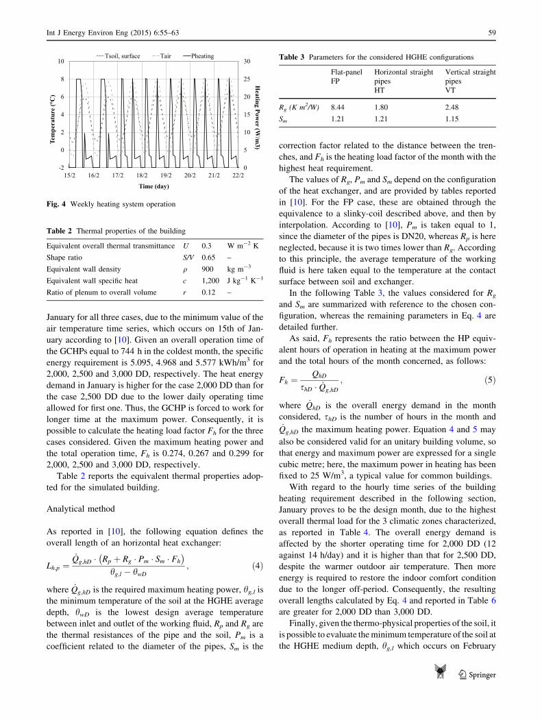
In the following Table 3, the values considered for Rg

and Sm are summarized with reference to the chosen con-

figuration, whereas the remaining parameters in Eq. 4 are

detailed further.

As said, Fh represents the ratio between the HP equiv-

alent hours of operation in heating at the maximum power

and the total hours of the month concerned, as follows:

Fh ¼ QhD

shD � _Qg;hD

; ð5Þ

where _QhD is the overall energy demand in the month

considered, shD is the number of hours in the month and_Qg;hD the maximum heating power. Equation 4 and 5 may

also be considered valid for an unitary building volume, so

that energy and maximum power are expressed for a single

cubic metre; here, the maximum power in heating has been

fixed to 25 W/m3, a typical value for common buildings.

With regard to the hourly time series of the building

heating requirement described in the following section,

January proves to be the design month, due to the highest

overall thermal load for the 3 climatic zones characterized,

as reported in Table 4. The overall energy demand is

affected by the shorter operating time for 2,000 DD (12

against 14 h/day) and it is higher than that for 2,500 DD,

despite the warmer outdoor air temperature. Then more

energy is required to restore the indoor comfort condition

due to the longer off-period. Consequently, the resulting

overall lengths calculated by Eq. 4 and reported in Table 6

are greater for 2,000 DD than 3,000 DD.

Finally, given the thermo-physical properties of the soil, it

is possible to evaluate the minimum temperature of the soil at

the HGHE medium depth, hg,l which occurs on February

0

5

10

15

20

25

30

-2

0

2

4

6

8

10

15/2 16/2 17/2 18/2 19/2 20/2 21/2 22/2

Heating Pow

er (W/m

3)Tem

pera

ture

(°C

)

Time (day)

Tsoil, surface Tair Pheating

Fig. 4 Weekly heating system operation

Table 2 Thermal properties of the building

Equivalent overall thermal transmittance U 0.3 W m-2 K

Shape ratio S/V 0.65 –

Equivalent wall density q 900 kg m-3

Equivalent wall specific heat c 1,200 J kg-1 K-1

Ratio of plenum to overall volume r 0.12 –

Table 3 Parameters for the considered HGHE configurations

Flat-panel

FP

Horizontal straight

pipes

HT

Vertical straight

pipes

VT

Rg (K m2/W) 8.44 1.80 2.48

Sm 1.21 1.21 1.15


123

15th. Therefore, the average temperature of the working fluid

hwD is chosen to be 6 K lower than hg,l for each climate zone,

according to the values suggested by [10].

In Table 5, the values for hwD and hg,l used in the ana-

lytical method are reported.

In order to make the analytical method comparable to

the numerical model, a procedure has been developed to

calculate the energy requirement at the heat exchanger for

unit length of trench. From Eq. (4), the length lh (mpipe/m3)

is calculated as the overall pipe length needed to meet the

energy demand of a building unit volume for each HGHEs,

according the assigned specific maximum heat power

(25 W/m3), heating requirements and other parameters.

Furthermore, the length of pipe available in a metre of

trench, LHGHE, is known for the various HGHEs configu-

rations. It is equal to 31.87 mpipe/mtrench for the FP case,

equivalent to 10.15 coils arranged on two levels having the

same FP heat transfer surface, while it is 8 mpipe/mtrench for

HT and VT. Therefore, the building heated volume per unit

length of trench vh (m3/mtrench) is calculated as the ratio

between LHGHE and lh.

Since the two-dimensional cross section simulated with

the numerical model is equivalent to a trench length of

1 m, vh is used as a multiplier for the time series of energy

requirement at the HGHE q(t), previously calculated with

Eq. (3). The heating system has been set to have a maxi-

mum power of 25 W/m3, hence the time series thus

obtained is characterized by an estimated maximum heat

extraction rates for unit of trench Qmax (W/m).

Results

Table 6 summarizes the values of lh, vh and Qmax adopted

for every heat exchanger and climate zone considered.

The resulting heat extraction rates for FP are 67.9, 69.7

and 62.3 W/m for 2,000, 2,500 and 3,000 DD, respectively.

For HT, the heat extraction rates are 78.3, 80.4 and 71.9,

whereas for VT they are 60.2, 61.8 and 55.2; thus, the HT

case is 15 % higher than FP, while VT is 11 % lower.

Although it is not the main purpose of this work, the dif-

ference in terms of heat extraction rate between the dif-

ferent HGHEs should be highlighted. This is linked mainly

to the design of each HGHE. FP and VT have similar

geometry but VT has a lower heat transfer surface area,

while HT, whose cross section is wider, is able to involve a

larger volume of soil. With regard to lh, it should be

remembered that every metre of FP is equivalent to

31.87 m of slinky-coil, so that the FP lengths are 0.37, 0.36

and 0.40 m for 2,000, 2,500 and 3,000 DD, for building

unit volume.

The results also show that, to achieve the same heating

power, the flat-panel requires a greater length of trench

than the horizontal tube exchangers, and a lower trench

length than the vertical ones. This is partly explained by the

larger amount of soil involved in the horizontal configu-

ration, due to the larger cross-section of HT. Despite the

higher efficiency in heat transfer rate, this results in higher

digging costs to build the trench. Moreover, the soil tem-

perature at the centre of the system for the horizontal

alignment drops to lower values than for the other cases.

However, neglecting the thermal resistance of the pipe wall

may penalize the performance of the flat-panel. The ther-

mal resistance is significantly lower for FP than for straight

pipe exchangers, due to the lower amount of material

consisting the FP for equal heat transfer surface. Thus, we

suppose that the flat-panel performance could be better

than those of the two other cases, finally.

The values of the daily average temperature at the wall of

the HGHEs are shown in Figs. 5, 6 and 7, for the different

configurations and the different climatic conditions. The

temperature used in the analytical method hwD is also

reported as benchmark. The temperature drops to its mini-

mum values around the middle of February, with a time shift

Table 4 Heating load factor in January

DD _QhD (Wh/m3) shD (h) _Qg;hD (W/m3) Fh (-)

2,000 5095.0 744 25 0.274

2,500 4968.3 744 25 0.267

3,000 5577.8 744 25 0.299

Table 5 Design values of

temperature�C 2,000

DD

2,500

DD

3,000

DD

hg;l 9.5 7.2 4.4

hwD 3.5 1.2 -1.4

Table 6 Resulting maximum heat extraction rate of the different

HGHEs

Case DD lh (mpipe/

m3)

L (mpipe/

mtrench)

vh (m3/

mtrench)

_Qmax (W/

mtrench)

FPa 2,000 11.725 31.87 2.718 67.9

2,500 11.425 31.87 2.789 69.7

3,000 12.790 31.87 2.492 62.3

HT 2,000 2.554 8.00 3.132 78.3

2,500 2.487 8.00 3.216 80.4

3,000 2.780 8.00 2.877 71.9

VT 2,000 3.321 8.00 2.409 60.2

2,500 3.237 8.00 2.471 61.8

3,000 3.620 8.00 2.209 55.2

a 31.87 mpipe are equivalent to 1 metre of FP


123

of about one month with respect to the minimum value of air

temperature. The minimum temperature with FP is only

0.3 �C lower than that evaluated by the analytical method.

This minor discrepancy is observed for all the three different

boundary conditions. This demonstrates that the approach

followed to size a flat-panel by means of the analytical

method is correct, albeit a negligible tendency to underesti-

mate the length of the heat exchanger is visible. In the other

two configurations (VT and HT), the average minimum

temperature is achieved as expected. The behaviour of VT

and HT is comparable, thus their relative difference is

negligible.

For completeness, a weekly detail of the hourly opera-

tion of the heat exchangers is shown in Figs. 8, 9 and 10,

when the minimum temperature is reached in the heating

period. All the HGHEs work around at the same minimum

temperature which is 2 K lower than the minimum daily

average temperature. Moreover, FP displays less pro-

nounced oscillations than HT and VT, with a lower capa-

bility of recovering. In fact, when the system is turned off

the temperature in HT and VT increases of 1.3 K more

than in FP.

Figures 11, 12 and 13 show the ground temperature for a

single measuring point placed on the domain axis of

symmetry, at the average depth of the system (0; -1.5 m).

The ground temperature for an undisturbed point, 10 m far

from the exchanger (14; -1.5 m) is included for com-

pleteness. The amount of energy extracted by HGHE dur-

ing the whole heating season is also shown. With reference

to 2,500 DD, the energy exploitation made by the FP

causes a decrease of the ground temperature of 3.6 �C in

comparison with the undisturbed point at the same depth.

The temperature drop is more pronounced, 4.1 �C, for the

HT configuration, due to its higher specific power and the

larger soil volume involved. On the contrary, the drop is

reduced of 0.4 �C for VT. The difference between the three

HGHEs remains almost unchanged for different boundary

conditions (2,000 and 3,000 DD). Given the different heat

extraction rate of the exchangers, the energy exploited

during the entire heating season in the 2,500 DD case is

-4-202468

10121416182022

15/10 14/11 14/12 13/1 12/2 14/3 13/4

Tem

pera

ture

(°C

)

Time (day)

FP HT VT

CwD °= 5.3θ

Fig. 5 Daily average temperature at the HGHE surface: 2,000 DD

-4-202468

10121416182022

15/10 14/11 14/12 13/1 12/2 14/3 13/4

Tem

pera

ture

(°C

)

Time (day)

FP HT VT

CwD °= 2.1θ


-4-202468

10121416182022

15/10 14/11 14/12 13/1 12/2 14/3 13/4

Tem

pera

ture

( °C

)

Time (day)

FP HT VT

CwD °−= 6.1θ


-4-3-2-10123456

15/2 16/2 17/2 18/2 19/2 20/2 21/2 22/2

Tem

pera

ture

(°C

)

Time (day)

FP HT VT

Fig. 8 Hourly temperature time series at the HGHE surface: 2,000

DD


123

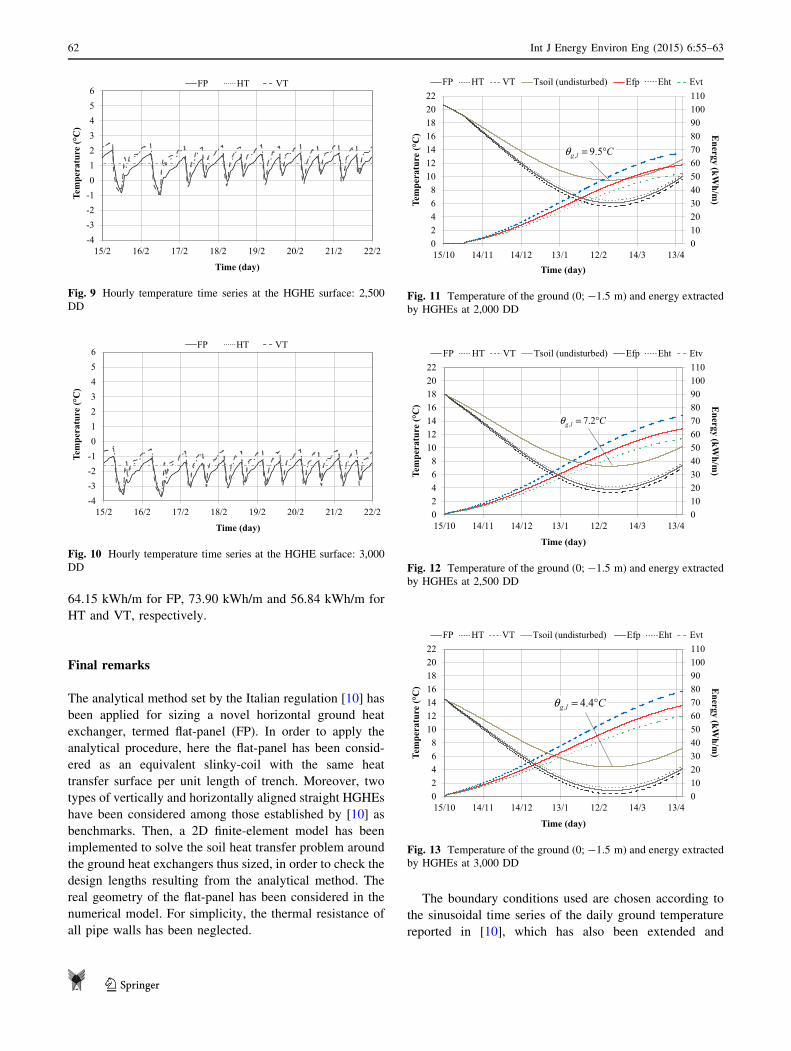
64.15 kWh/m for FP, 73.90 kWh/m and 56.84 kWh/m for

HT and VT, respectively.

Final remarks

The analytical method set by the Italian regulation [10] has

been applied for sizing a novel horizontal ground heat

exchanger, termed flat-panel (FP). In order to apply the

analytical procedure, here the flat-panel has been consid-

ered as an equivalent slinky-coil with the same heat

transfer surface per unit length of trench. Moreover, two

types of vertically and horizontally aligned straight HGHEs

have been considered among those established by [10] as

benchmarks. Then, a 2D finite-element model has been

implemented to solve the soil heat transfer problem around

the ground heat exchangers thus sized, in order to check the

design lengths resulting from the analytical method. The

real geometry of the flat-panel has been considered in the

numerical model. For simplicity, the thermal resistance of

all pipe walls has been neglected.

The boundary conditions used are chosen according to

the sinusoidal time series of the daily ground temperature

reported in [10], which has also been extended and

-4-3-2-10123456

15/2 16/2 17/2 18/2 19/2 20/2 21/2 22/2

Tem

pera

ture

(°C

)

Time (day)

FP HT VT


DD

-4-3-2-10123456

15/2 16/2 17/2 18/2 19/2 20/2 21/2 22/2

Tem

pera

ture

(°C

)

Time (day)

FP HT VT


DD

0102030405060708090100110

02468

10121416182022

15/10 14/11 14/12 13/1 12/2 14/3 13/4

Energy (kW

h/m)Te

mpe

ratu

re (°

C)

Time (day)

FP HT VT Tsoil (undisturbed) Efp Eht Evt

Clg °= 5.9,θ

Fig. 11 Temperature of the ground (0; -1.5 m) and energy extracted

by HGHEs at 2,000 DD

0102030405060708090100110

02468

10121416182022

15/10 14/11 14/12 13/1 12/2 14/3 13/4

Energy (kW

h/m)Te

mpe

ratu

re (°

C)

Time (day)

FP HT VT Tsoil (undisturbed) Efp Eht Etv

Clg °= 2.7,θ



0102030405060708090100110

02468

10121416182022

15/10 14/11 14/12 13/1 12/2 14/3 13/4

Energy (kW

h/m)Te

mpe

ratu

re (°

C)

Time (day)

FP HT VT Tsoil (undisturbed) Efp Eht Evt

Clg °= 4.4,θ




123

synchronized to the air temperature. Further detail in the

forcing term has been added upon superimposing an

additional sinusoidal function describing the hourly tem-

perature variation. These boundary conditions have been

applied to evaluate the heating requirements of a simplified

lumped system representing a typical building.

The results of the analytical method match those of the

numerical model, in terms of minimum temperature at the

interface between heat exchanger and soil. It should be

pointed out that the minimum temperature in FP is slightly

lower than that expected; however, the resulting under-

sizing is negligible. Thus, the proposed approach to size a

flat-panel by means of an analytical procedure has proven

to be effective for each boundary condition considered.

Open Access This article is distributed under the terms of the

Creative Commons Attribution License which permits any use, dis-

tribution, and reproduction in any medium, provided the original

author(s) and the source are credited.

References

1. Mustaf, O.A.: Ground-source heat pumps systems and applica-

tions. Renew. Sustain. Energy Rev. 12(2), 344–371 (2008)

2. Chiasson, A.D.: Advances in modeling of ground-source heat

pump systems. M.Sc. Thesis, Oklahoma State University, Okla-

homa (1999)

3. Gan, G.: Dynamic thermal modeling of horizontal ground-source

heat pumps. Int. J. Low-Carbon Technol. 8, 95–105 (2013)

4. Fujii, H., Yamasaki, S., Maehara, T., Ishikami, T., Chou, N.:

Numerical simulation and sensitivity study of double-layer

Slinky-coil horizontal ground heat exchangers. Geothermics 47,

61–68 (2013)

5. Bottarelli, M., Di Federico, V.: Numerical comparison between

two advanced HGHEs. Int. J. Low Carbon Technol. 7, 75–81

(2012)

6. Bottarelli, M.: A preliminary testing of a flat panel ground heat

exchanger. Int. J. Low Carbon Technol. 8, 80–87 (2013)

7. Collins, P.A., Orio, C.D., Smiriglio, S.: Geothermal Heat Pump

Manual. NYC Department of Design & Construction, New York

(2002)

8. Kavanaugh, S.P., Rafferty, K.: Ground Source Heat Pumps-

design of Geothermal Systems for Commercial and Institutional

Buildings. ASHRAE Applications Handbook (1997)

9. IGSHPA: Ground Source Heat Pump Residential and Light

Commercial Design and Installation Guide. Oklahoma State

University, Stillwater (2009)

10. UNI 11466: Heat Pump Geothermal Systems: Design and Sizing

Requirements (2012)

11. Congedo, P.M., Colangelo, G., Starace, G.: CFD simulations of

horizontal ground heat exchangers: a comparison among different

configurations. Appl. Therm. Eng. 33–34, 24–32 (2012)

12. Fujii, H., Nishi, K., Komaniwa, Y., Chou, N.: Numerical mod-

eling of slinky-coil horizontal ground heat exchangers. Geother-

mics 41, 55–62 (2012)

13. Piechowsky, M.: Heat and mass transfer model of a ground heat

exchanger: validation and sensitivity analysis. Int. J. Energy Res.

23, 571–588 (1999)

14. Demir, H., Koyun, A., Temir, G.: Heat transfer of horizontal

parallel pipe ground heat exchanger and experimental verifica-

tion. Appl. Therm. Eng. 29, 224–233 (2009)

15. Simms, R.B., Haslam, S.R., Craig, J.R.: Impact of soil heterog-

enity on the functioning of horizontal ground heat exchanger.

Geothermics 50, 35–43 (2013)

16. Carslaw, H.S., Jaeger, J.C.: Conduction of Heat in Solids. Oxford

University Press, New York (1959)

17. Bottarelli, M., Di Federico, V.: Adoption of flat panels in soil heat

exchange. Proceedings of 11th World Renewable Energy Con-

gress, 330–335 (2010)

18. Bottarelli, M., Gabrielli, L.: Payback period for a ground source

heat pump system. Int. J. Heat Technol. 29(2), 145–150 (2011)


123

Documents

On the sizing of a ﬂat-panel ground heat exchanger