On the Power of (even a little) Centralization in DistributedProcessing *

John N. Tsitsiklis

MIT, LIDSCambridge, MA 02139

jnt@mit.edu

Kuang Xu

MIT, LIDSCambridge, MA 02139kuangxu@mit.edu

ABSTRACTWe propose and analyze a multi-server model that capturesa performance trade-off between centralized and distributedprocessing. In our model, a fraction p of an available re-source is deployed in a centralized manner (e.g., to serve amost-loaded station) while the remaining fraction 1 − p isallocated to local servers that can only serve requests ad-dressed specifically to their respective stations.

Using a fluid model approach, we demonstrate a surpris-ing phase transition in the steady-state delay, as p changes:in the limit of a large number of stations, and when anyamount of centralization is available (p > 0), the averagequeue length in steady state scales as log 1

1−p

11−λ when the

traffic intensity λ goes to 1. This is exponentially smallerthan the usual M/M/1-queue delay scaling of 1

1−λ , obtainedwhen all resources are fully allocated to local stations (p = 0).This indicates a strong qualitative impact of even a smalldegree of centralization.

We prove convergence to a fluid limit, and characterizeboth the transient and steady-state behavior of the finitesystem, in the limit as the number of stations N goes to in-finity. We show that the sequence of queue-length processesconverges to a unique fluid trajectory (over any finite timeinterval, as N →∞), and that this fluid trajectory convergesto a unique invariant state vI , for which a simple closed-formexpression is obtained. We also show that the steady-statedistribution of the N -server system concentrates on vI as Ngoes to infinity.

Categories and Subject DescriptorsG.3 [Probability and Statistics]: Queuing theory, Markovprocesses; C.2.1 [Network Architecture and Design]:Centralized networks, Distributed networks

General TermsPerformance, Theory

* This technical report is an extended version of the conference paper pre-sented at ACM Sigmetrics 2011 [1], with additional proofs included in theAppendix. Research supported in part by an MIT Jacobs Presidential Fellowship,an MIT-Xerox Fellowship, a Siebel Scholarship, and NSF grant CCF-0728554. The authors are grateful to Yuan Zhong for a careful readingof the manuscript and his comments.

KeywordsPhase transition, Dynamic resource allocation, Partial cen-tralization

1. INTRODUCTIONThe tension between distributed and centralized process-

ing seems to have existed ever since the inception of com-puter networks. Distributed processing allows for simpleimplementation and robustness, while a centralized schemeguarantees optimal utilization of computing resources at thecost of implementation complexity and communication over-head. A natural question is how performance varies withthe degree of centralization. Such understanding is of greatinterest in the context of, for example, infrastructure plan-ning (static) or task scheduling (dynamic) in large serverfarms or cloud clusters, which involve a trade-off betweenperformance (e.g., delay) and cost (e.g., communication in-frastructure, energy consumption, etc.). In this paper, weaddress this problem by formulating and analyzing a multi-server model with an adjustable level of centralization. Webegin by describing informally two motivating applications.

1.1 Primary Motivation: Server Farm with Lo-cal and Central Servers

Consider a server farm consisting of N stations, depictedin Figure 1. Each station is fed by an independent streamof tasks, arriving at a rate of λ tasks per second, with 0 <λ < 1.1 Each station is equipped with a local server withidentical performance; the server is local in the sense that itonly serves its own station. All stations are also connectedto a single centralized server which will serve a station withthe longest queue whenever possible.

We consider an N -station system. The system designer isgranted a total amount of N divisible computing resources(e.g., a collection of processors). In a loose sense (to beformally defined in Section 2.1), this means that the sys-tem is capable of processing N tasks per second when fullyloaded. The system designer is faced with the problem ofallocating computing resources to local and central servers.Specifically, for some p ∈ (0,1), each of the N local serversis able to process tasks at a maximum rate of 1 − p tasksper second, while the centralized server, equipped with theremaining computing power, is capable of processing tasksat a maximum rate of pN tasks per second. The parameterp captures the amount of centralization in the system. Note

1Without loss of generality, we normalize so that the largest pos-sible arrival rate is 1.

that since the total arrival rate is λN , with 0 < λ < 1, thesystem is underloaded for any value p ∈ (0,1).

When the arrival process and task processing times arerandom, there will be times when some stations are emptywhile others are loaded. Since a local server cannot helpanother station process tasks, the total computational re-sources will be better utilized if a larger fraction is allo-cated to the central server. However, a greater degree ofcentralization (corresponding to a larger value of p) entailsmore frequent communications and data transfers betweenthe local stations and the central server, resulting in higherinfrastructure and energy costs.

How should the system designer choose the coefficient p?Alternatively, we can ask an even more fundamental ques-tion: is there any significant difference between having asmall amount of centralization (a small but positive valueof p), and complete decentralization (no central server andp = 0)?

1.2 Secondary Motivation: Partially Central-ized Scheduling

Consider the system depicted in Figure 2. The arrivalassumptions are the same as in the Section 1.1. However,there is no local server associated with a station; all stationsare served by a single central server. Whenever the centralserver becomes free, it chooses a task to serve as follows.With probability p, it processes a task from a most loadedstation. Otherwise, it processes a task from a station se-lected uniformly at random; if the randomly chosen stationis empty, the current round is in some sense “wasted” (to beformalized in Section 2.1).

This second interpretation is intended to model a scenariowhere resource allocation decisions are made at a central-ized location on a dynamic basis, but communications be-tween the decision maker (central server) and local stationsare costly or simply unavailable from time to time. Hence,while it is intuitively obvious that longest-queue-first (LQF)scheduling is more desirable, it may not always be possibleto obtain up-to-date information on the system state (i.e.,the queue lengths at all stations). Thus, the central servermay be forced to allocate service blindly. In this setting,a system designer is interested in setting the optimal fre-quency (p) at which global state information is collected soas to balance performance and communication costs.

As we will see in the sequel, the system dynamics in thetwo applications are captured by the same mathematicalstructure under appropriate stochastic assumptions on taskarrivals and processing times, and hence will be addressedjointly in the current paper.

1.3 Overview of Main ContributionsWe provide here an overview of the main contributions.

Exact statements of our results will be provided in Section3 after the necessary terminology has been introduced.

Our goal is to study the performance implications of vary-ing degrees of centralization, as expressed by the coefficientp. To accomplish this, we use a so-called fluid approxima-tion, whereby the queue length dynamics at the local sta-tions are approximated, as N →∞, by a deterministic fluidmodel, governed by a system of ordinary differential equa-tions (ODEs).

Fluid approximations typically lead to results of two fla-vors: qualitative results derived from the fluid model that

Figure 1: Server Farm with Local and CentralServers

Figure 2: Centralized Scheduling with Communica-tion Constraints

give insights into the performance of the original finitestochastic system, and technical convergence results (oftenmathematically involved) that justify the use of such ap-proximations. We summarize our contributions along thesetwo dimensions:

1. On the qualitative end, we derive an exact expres-sion for the invariant state of the fluid model, for anygiven traffic intensity λ and centralization coefficientp, thus characterizing the steady-state distribution ofthe queue lengths in the system as N → ∞. This en-ables a system designer to use any performance metricand analyze its sensitivity with respect to p. In par-ticular, we show a surprising exponential phase transi-tion in the scaling of average system delay as the loadapproaches capacity (λ → 1) (Corollary 3): when anarbitrarily small amount of centralized computation isapplied (p > 0), the average queue length in the systemscales as 2

E(Q) ∼ log 11−p

1

1 − λ, (1)

as the traffic intensity λ approaches 1. This is dras-tically smaller than the 1

1−λ scaling obtained if there

is no centralization (p = 0).3 In terms of the questionraised at the end of Section 1.1, this suggests that for

2The ∼ notation used in this paper is to be understood as asymp-totic closeness in the following sense: f (x) ∼ g (x) , as x → 1⇔

limx→1f(x)g(x) = 1.

3When p = 0, the system degenerates into N independent queues.The 1

1−λ scaling comes from the mean queue length expression

for M/M/1 queues.

large systems, even a small degree of centralization in-deed provides significant improvements in the system’sdelay performance, in the heavy traffic regime.

2. On the technical end, we show:

(a) Given any finite initial queue sizes, and with highprobability, the evolution of the queue length pro-cess can be approximated by the unique solutionto a fluid model, over any finite time interval, asN →∞.

(b) All solutions to the fluid model converge to aunique invariant state, as time t → ∞, for anyfinite initial condition (global stability).

(c) The steady-state distribution of the finite systemconverges to the invariant state of the fluid modelas N →∞.

The most notable technical challenge comes from thefact that the longest-queue-first policy used by the cen-tralized server causes discontinuities in the drift in thefluid model (see Section 3.1 for details). In partic-ular, the classical approximation results for Markovprocesses (see, e.g., [3]), which rely on a Lipschitz-continuous drift in the fluid model, are hard to ap-ply. Thus, in order to establish the finite-horizon ap-proximation result (a), we employ a sample-path basedapproach: we prove tightness of sample paths of thequeue length process and characterize their limit points.Establishing the convergence of steady state distribu-tions in (c) also becomes non-trivial due to the pres-ence of discontinuous drifts. To derive this result, wewill first establish the uniqueness of solutions to thefluid model and a uniform speed of convergence ofstochastic sample paths to the solution of the fluidmodel over a compact set of initial conditions.

1.4 Related WorkTo the best of our knowledge, the proposed model for

the splitting of computing resources between distributed andcentral servers has not been studied before. However, thefluid model approach used in this paper is closely related to,and partially motivated by, the so-called supermarket modelof randomized load-balancing. In that literature, it is shownthat by routing tasks to the shorter queue among a smallnumber (d ≥ 2) of randomly chosen queues, the probabilitythat a typical queue has at least i tasks (denoted by si) de-

cays as λdi−1d−1 (super-geometrically) as i → ∞ ([4],[5]); see

also the survey paper [9] and references therein. A varia-tion of this approach in a scheduling setting with channeluncertainties is examined in [6], but si no longer exhibitssuper-geometric decay and only moderate performance gaincan be harnessed from sampling more than one queue.

In our setting, the system dynamics causing the exponen-tial phase transition in the average queue length scaling aresignificantly different from those for the randomized load-balancing scenario. In particular, for any p > 0, the tailprobabilities si become zero for sufficiently large finite i,which is significantly faster than the super-geometric decayin the supermarket model.

On the technical side, arrivals and processing times usedin supermarket models are often memoryless (Poisson orBernoulli) and the drifts in the fluid model are typically con-tinuous with respect to the underlying system state. Hence

convergence results can be established by invoking classi-cal approximation results, based on the convergence of thegenerators of the associated Markov processes. An excep-tion is [8], where the authors generalized the supermarketmodel to arrival and processing times with general distribu-tions. Since the queue length process is no longer Markov,the authors reply on an asymptotic independence propertyof the limiting system and use tools from statistical physicsto establish convergence.

Our system remains Markov with respect to the queuelengths, but a significant technical difference from the su-permarket model lies in the fact that the longest-queue-firstservice policy introduces discontinuities in the drifts. Forthis reason, we need to use a more elaborate set of tech-niques to establish the connection between stochastic sam-ple paths and the fluid model. Moreover, the presence ofdiscontinuities in the drifts creates challenges even for prov-ing the uniqueness of solutions for the deterministic fluidmodel. (Such uniqueness is needed to establish convergenceof steady-state distributions.) Our approach is based on astate representation that is different from the one used inthe popular supermarket models, which turns out to be sur-prisingly more convenient to work with for establishing theuniqueness of solutions to the fluid model.

Besides the queueing-theoretic literature, similar fluid mo-del approaches have been used in many other contexts tostudy systems with large populations. Recent results in[7] establish convergence results for finite-dimensional sym-metric dynamical systems with drift discontinuities, usinga more probabilistic (as opposed to sample path) analysis,carried out in terms of certain conditional expectations. Webelieve it is possible to prove our results using the meth-ods in [7], with additional work. However, the coupling ap-proach used in this paper provides strong physical intuitionon the system dynamics, and avoids the need for additionaltechnicalities from the theory of multi-valued differential in-clusions.

Finally, there has been some work on the impact of serviceflexibilities in routing problems motivated by applicationssuch as multilingual call centers. These date back to theseminal work of [10], with a more recent numerical study in[11]. These results show that the ability to route a portionof customers to a least-loaded station can lead to a constant-factor improvement in average delay under diffusion scaling.This line of work is very different from ours, but in a broadersense, both are trying to capture the notion that system per-formance in a random environment can benefit significantlyfrom even a small amount of centralized coordination.

1.5 Organization of the PaperSection 2 introduces the precise model to be studied, our

assumptions, and the notation to be used throughout. Themain results are summarized in Section 3, where we alsodiscuss their implications along with some numerical results.The remainder of the paper is devoted to proofs, and thereader is referred to Section 4 for an overview of the proofstructure. Due to space limitations, some of the proofs aresketched, omitted, or relegated to the Appendix.

2. MODEL AND NOTATION

2.1 ModelWe present our model using terminology that corresponds

to the server farm application in Section 1.1. Time is as-sumed to be continuous.

1. System. The system consists of N parallel stations.Each station is associated with a queue which storesthe tasks to be processed. The queue length (i.e., num-ber of tasks) at station n at time t is denoted by Qn(t),n ∈ 1,2, . . . ,N, t ≥ 0. For now, we do not make anyassumptions on the queue lengths at time t = 0, otherthan that they are finite.

2. Arrivals. Stations receive streams of incoming tasksaccording to independent Poisson processes with a com-mon rate λ ∈ [0,1).

3. Task Processing. We fix a centralization coefficientp ∈ [0,1].

(a) Local Servers. The local server at station n ismodeled by an independent Poisson clock withrate 1 − p (i.e., the times between two clock ticksare independent and exponentially distributed withmean 1

1−p ). If the clock at station n ticks at time

t, we say that a local service token is generatedat station n. If Qn(t) ≠ 0, exactly one task fromstation n “consumes” the service token and leavesthe system immediately. Otherwise, the local ser-vice token is “wasted” and has no impact on thefuture evolution of the system.4

(b) Central Server. The central server is modeledby an independent Poisson clock with rate Np.If the clock ticks at time t at the central server,we say that a central service token is gen-erated. If the system is non-empty at t (i.e.,∑Nn=1Qn(t) > 0), exactly one task from some sta-tion i, chosen uniformly at random out of the sta-tions with a longest queue at time t, consumes theservice token and leaves the system immediately.If the whole system is empty, the central servicetoken is wasted.

Equivalence between the two motivating applica-tions. We comment here that the scheduling application inSection 1.2 corresponds to the same mathematical model.The arrival statistics to the stations are obviously identi-cal in both models. For task processing, note that we canequally imagine all service tokens as being generated froma single Poisson clock with rate N . Upon the generationof a service token, a coin is flipped to decide whether thetoken will be directed to process a task at a random station(corresponding to a local service token), or a station witha longest queue (corresponding to a central service token).Due to the Poisson splitting property, this produces identi-cal statistics for the generation of local and central servicetokens as described above.

4The generation of a token can also be thought of as a completionof a previous task, so that the server “fetches” a new task fromthe queue to process, hence decreasing the queue length by 1.The same interpretation holds for the central service tokens. SeeSection 2.1 of [13] for a discussion on the physical interpretationof service tokens.

2.2 System StateLet us fix N . Since all events (arrivals of tasks and ser-

vice tokens) are generated according to independent Poissonprocesses, the queue length vector at time t, (Q1(t),Q2(t),. . . ,QN(t)), is Markov. Moreover, the system is fully sym-metric, in the sense that all queues have identical and inde-pendent statistics for the arrivals and local service tokens,and the assignment of central service tokens does not de-pend on the specific identity of stations besides their queuelengths. Hence we can use a Markov process SNi (t)∞

i=0 todescribe the evolution of a system with N stations, where

SNi (t) = 1

N

N

∑n=1

I[i,∞) (Qn(t)) , i ≥ 0. (2)

Each coordinate SNi (t) represents the fraction of queueswith at least i tasks. Note that SN0 (t) = 1 for all t andN according to this definition. We call SN (t) the normal-ized queue length process. We also define the aggregatequeue length process as

VNi (t) =

∞∑j=i

SNj (t) , i ≥ 0. (3)

Note that

SNi (t) = VNi (t) −VN

i+1(t). (4)

In particular, this means that VN0 (t) −VN

1 (t) = SN0 (t) = 1.Note also that

VN1 (t) =

∞∑j=1

SNj (t) (5)

is equal to the average queue length in the system at time t.When the total number of tasks in the system is finite (henceall coordinates of VN(t) are finite), there is a straightfor-ward bijection between SN(⋅) and VN(⋅). Hence VN(t)is Markov and also serves as a valid representation of thesystem state. While the SN representation admits a moreintuitive interpretation as the “tail” probability of a typicalstation having at least i tasks, it turns out the VN(⋅) rep-resentation is significantly more convenient to work with,especially in proving uniqueness of solutions to the associ-ated fluid model (see Section 7.1). For this reason, we willbe working mostly with the VN representation, but will insome places state results in terms of SN , if doing so providesa better physical intuition.

2.3 NotationLet Z+ be the set of non-negative integers. The following

sets will be used throughout the paper (whereM is a positiveinteger):

S = s ∈ [0,1]Z+ ∶ 1 = s0 ≥ s1 ≥ ⋯ ≥ 0 , (6)

SM = s ∈ S ∶∞∑i=1

si ≤M , S∞ = s ∈ S ∶∞∑i=1

si <∞ , (7)

VM =⎧⎪⎪⎨⎪⎪⎩v ∶ vi =

∞∑j=i

sj , for some s ∈ SM⎫⎪⎪⎬⎪⎪⎭, (8)

V∞ =⎧⎪⎪⎨⎪⎪⎩v ∶ vi =

∞∑j=i

sj , for some s ∈ S∞⎫⎪⎪⎬⎪⎪⎭, (9)

QN = x ∈ RZ+ ∶ xi =K

N, for some K ∈ Z+,∀i . (10)

We define the weighted L2 norm ∥ ⋅ ∥w on RZ+ as

∥x − y∥2w =

∞∑i=0

∣xi − yi∣2

2i, x,y ∈ RZ+ . (11)

In general, we will be using bold letters to denote vectorsand ordinary letters for scalars, with the exception that abold letter with a subscript (e.g., vi) is understood as a(scalar-valued) component of a vector. Upper-case letters

are generally reserved for random variables (e.g., V(0,N))or scholastic processes (e.g., VN(t)), and lower-case lettersare used for constants (e.g., v0) and deterministic functions(e.g., v(t)). Finally, a function is in general denoted by x(⋅),but is sometimes written as x(t) to emphasize the type ofits argument.

3. SUMMARY OF MAIN RESULTS

3.1 Definition of Fluid ModelBefore introducing the main results, we first define the

fluid model, with some intuitive justification.

Definition 1. (Fluid Model) Given an initial condition

v0 ∈ V∞, a function v(t) ∶ [0,∞) → V∞ is said to be asolution to the fluid model (or fluid solution for short)if:

(1) v(0) = v0;

(2) for all t ≥ 0,

v0(t) − v1(t) = 1, (12)

and 1 ≥ vi(t) − vi+1(t) ≥ vi+1(t) − vi+2(t) ≥ 0, ∀i ;(13)

(3) for almost all t ∈ [0,∞), and for every i ≥ 1, vi(t) isdifferentiable and satisfies

vi (t) = λ (vi−1 − vi) − (1 − p) (vi − vi+1) − gi (v) , (14)

where

gi (v) =⎧⎪⎪⎪⎨⎪⎪⎪⎩

p, vi > 0,minλvi−1, p , vi = 0,vi−1 > 0,0, vi = 0,vi−1 = 0.

(15)

We can write Eq. (14) more compactly as

v (t) = F (v) , (16)

where

Fi (v) = λ (vi−1 − vi) − (1 − p) (vi − vi+1) − gi (v) . (17)

We call F (v) the drift at point v.

Interpretation of the fluid model.The solution to thefluid model, v(t), can be thought of as a deterministic ap-proximation to the sample paths of VN(t) for large values ofN . Conditions (1) and (2) correspond to initial and bound-ary conditions, respectively. Before rigorously establishingthe validity of approximation, we provide some intuition foreach of the drift terms in Eq. (14):

I. λ (vi−1 − vi): This term corresponds to arrivals. Whena task arrives at a station with i−1 tasks, the system has onemore queue with i tasks, and SNi increases by 1

N. However,

the number of queues with at least j tasks, for j ≠ i, does

not change. Thus, SNi is the only one that is incremented.

Since VNi

= ∑∞k=i S

Nk , this implies that VN

i is increased by1N

if and only if a task arrives at a queue with at least i− 1tasks. Since all stations have an identical arrival rate λ,the probability of VN

i being incremented upon an arrival tothe system is equal to the fraction of queues with at leasti − 1 tasks, which is VN

i−1(t) −VNi (t). We take the limit as

N → ∞, and multiply by the total arrival rate, Nλ, timesthe increment due to each arrival, 1

N, to obtain the term

λ (vi−1 − vi).II. (1 − p) (vi − vi+1): This term corresponds to the com-

pletion of tasks due to local service tokens. The argumentis similar to that for the first term.

III. gi (v): This term corresponds to the completion oftasks due to central service tokens.

1. gi (v) = p, if vi > 0. If i > 0 and vi>0, then thereis a positive fraction of queues with at least i tasks.Hence the central server is working at full capacity,and the rate of decrease in vi due to central servicetokens is equal to the maximum rate of the centralserver, namely p.

2. gi (v) = minλvi−1, p , if vi = 0,vi−1 > 0. This caseis more subtle. Note that since vi = 0, the term λvi−1is equal to λ(vi−1 − vi), which is the rate at which viincreases due to arrivals. Here the central server servesqueues with at least i tasks whenever such queues ariseto keep vi at zero. Thus, the total rate of centralservice tokens dedicated to vi matches exactly the rateof increase of vi due to arrivals.5

3. gi (v) = 0, if vi = vi−1 = 0. Here, both vi and vi−1 arezero and there are no queues with i − 1 or more tasks.Hence there is no positive rate of increase in vi due toarrivals. Accordingly, the rate at which central servicetokens are used to serve stations with at least i tasksis zero.

Note that, as mentioned in the introduction, the disconti-nuities in the fluid model come from the term g(v), whichreflects the presence of a central server.

3.2 Analysis of the Fluid ModelThe following theorem characterizes the invariant state for

the fluid model. It will be used to demonstrate an exponen-tial improvement in the rate of growth of the average queuelength as λ→ 1 (Corollary 3).

Theorem 2. The drift F(⋅) in the fluid model admits a

unique invariant state vI (i.e., F(vI) = 0). Letting sIi=

vIi −vIi+1 for all i ≥ 0, the exact expression for the invariantstate as follows:

(1) If p = 0, then sIi = λi, ∀i ≥ 1.

(2) If p ≥ λ, then sIi = 0, ∀i ≥ 1.

5Technically, the minimization involving p is not necessary: ifλvi−1(t) > p, then vi(t) cannot stay at zero and will immediatelyincrease after t. We keep the minimization just to emphasize thatthe maximum rate of increase in vi due to central service tokenscannot exceed the central service capacity p.

(3) If 0 < p < λ, and λ = 1 − p, then6

sIi =⎧⎪⎪⎨⎪⎪⎩

1 − ( p1−p) i, 1 ≤ i ≤ i∗ (p, λ) ,

0, i > i∗ (p, λ) ,

where i∗ (p, λ) = ⌊ 1−pp

⌋.

(4) If 0 < p < λ, and λ ≠ 1 − p, then

sIi =⎧⎪⎪⎨⎪⎪⎩

1−λ1−(p+λ) ( λ

1−p)i− p

1−(p+λ) , 1 ≤ i ≤ i∗ (p, λ) ,0, i > i∗ (p, λ) ,

where

i∗ (p, λ) = ⌊log λ1−p

p

1 − λ⌋ , (18)

Proof. The proof consists of simple algebra to computethe solution to F(vI) = 0. The proof is given in AppendixA.1. ◻

Case (4) in the above theorem is particularly interesting,as it reflects the system’s performance under heavy load (λclose to 1). Note that since sI1 represents the probability ofa typical queue having at least i tasks, the quantity

vI1=

∞∑i=1

sIi (19)

represents the average queue length. The following corollary,which characterizes the average queue length in the invariantstate for the fluid model, follows from Case (4) in Theorem2 by some straightforward algebra.

Corollary 3. (Phase Transition in Average QueueLength Scaling) If 0 < p < λ and λ ≠ 1 − p, then

vI1=

∞∑i=1

sIi = (1 − p) (1 − λ)(1 − p − λ)2

⎡⎢⎢⎢⎣1 − ( λ

1 − p)i∗(p,λ)⎤⎥⎥⎥⎦

− p

1 − p − λi∗ (p, λ) , (20)

with i∗ (p, λ) = ⌊log λ1−p

p1−λ⌋. In particular, this implies that

for any fixed p > 0, vI1 scales as

vI1 ∼ i∗ (p, λ) ∼ log 11−p

1

1 − λ, as λ→ 1. (21)

The scaling of the average queue length in Eq. (21) withrespect to arrival rate λ is contrasted with (and is exponen-tially better than) the familiar 1

1−λ scaling when no central-ized resource is available (p = 0).

Intuition for Exponential Phase Transition. Theexponential improvement in the scaling of vI1 is surprising,because the expressions for sIi look ordinary and do not con-tain any super-geometric terms in i. However, a closer lookreveals that for any p > 0, the tail probabilities sI have afinite support: sIi “dips”down to 0 as i increases to i∗(p, λ),which is even faster than a super-geometric decay. Since

0 ≤ sIi ≤ 1 for all i, it is then intuitive that vI1 = ∑i∗(p,λ)i=1 sIi

is upper-bounded by i∗(p, λ), which scales as log 11−p

11−λ as

λ → 1. Note that a tail probability with “finite-support”implies that the fraction of stations with more than i∗(p, λ)6Here ⌊x⌋ is defined as the largest integer that is less than orequal to x.

10 20 30 40 50 60 700

0.2

0.4

0.6

0.8

1

i

Tai

l Pro

b. (

sI )

p=0p=0.05

i*(p,λ)

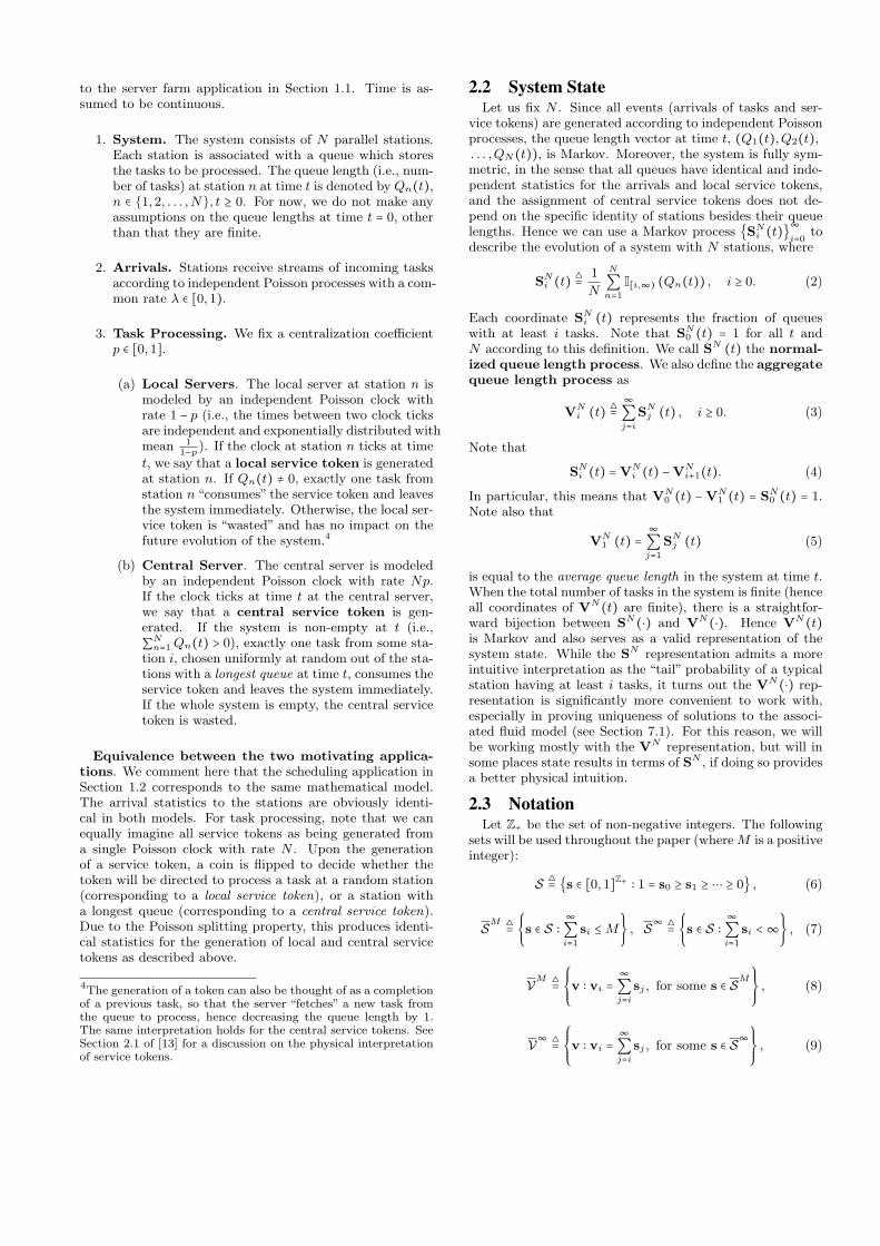
Figure 3: Values of sIi , as a function of i, for p = 0and p = 0.05, with traffic intensity λ = 0.99.

tasks decreases to zero asN →∞. For example, we may havea strictly positive fraction of stations with, say, 10 tasks, butstations with more than 10 tasks hardly exist. While thismay appear counterintuitive, it is a direct consequence ofcentralization in the resource allocation schemes. Since afraction p of the total resource is constantly going after thelongest queues, it is able to prevent long queues (i.e., queueswith more than i∗(p, λ) tasks) from even appearing. Thethresholds i∗(p, λ) increasing to infinity as λ → 1 reflectsthe fact that the central server’s ability to annihilate longqueues is compromised by the heavier traffic loads; our resultessentially shows that the increase in i∗(λ, p) is surprisinglyslow.

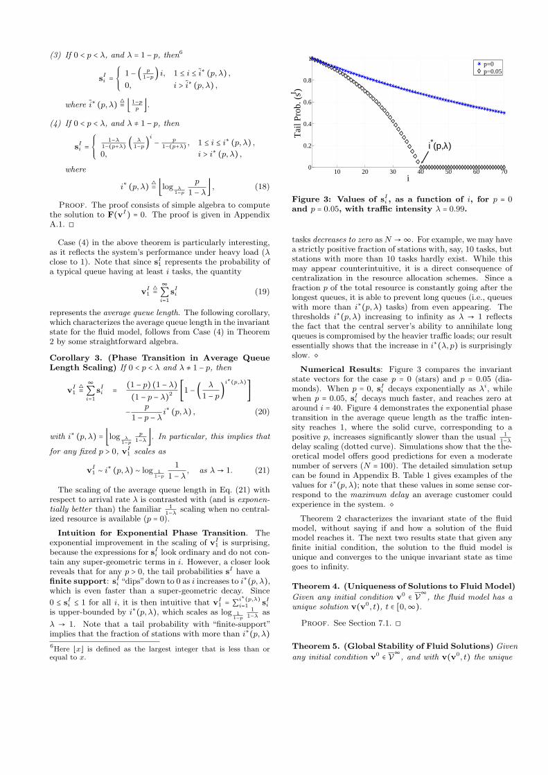
Numerical Results: Figure 3 compares the invariantstate vectors for the case p = 0 (stars) and p = 0.05 (dia-monds). When p = 0, sIi decays exponentially as λi, whilewhen p = 0.05, sIi decays much faster, and reaches zero ataround i = 40. Figure 4 demonstrates the exponential phasetransition in the average queue length as the traffic inten-sity reaches 1, where the solid curve, corresponding to apositive p, increases significantly slower than the usual 1

1−λdelay scaling (dotted curve). Simulations show that the the-oretical model offers good predictions for even a moderatenumber of servers (N = 100). The detailed simulation setupcan be found in Appendix B. Table 1 gives examples of thevalues for i∗(p, λ); note that these values in some sense cor-respond to the maximum delay an average customer couldexperience in the system.

Theorem 2 characterizes the invariant state of the fluidmodel, without saying if and how a solution of the fluidmodel reaches it. The next two results state that given anyfinite initial condition, the solution to the fluid model isunique and converges to the unique invariant state as timegoes to infinity.

Theorem 4. (Uniqueness of Solutions to Fluid Model)

Given any initial condition v0 ∈ V∞, the fluid model has aunique solution v(v0, t), t ∈ [0,∞).

Proof. See Section 7.1. ◻

Theorem 5. (Global Stability of Fluid Solutions) Given

any initial condition v0 ∈ V∞, and with v(v0, t) the unique

0.951 0.958 0.965 0.971 0.978 0.985 0.991 0.9980

100

200

300

400

500

600

Traffic Intensity (λ)

Ave

rage

Que

ue L

engt

h

p=0, by Theorem 2 (numerical) p=0.05, by Theorem 2 (numerical) p=0.05, N=100, by simulationwith 95% confidence intervals

Figure 4: Illustration of the exponential improve-ment in average queue length from O( 1

1−λ) to

O(log 11−λ) as λ→ 1, when we compare p = 0 to p = 0.05.

p = / λ = 0.1 0.6 0.9 0.99 0.9990.002 2 10 37 199 6920.02 1 6 18 68 1560.2 0 2 5 14 230.5 0 1 2 5 80.8 0 0 1 2 4

Table 1: Values of i∗(p, λ) for various combinationsof (p, λ).

solution to the fluid model, we have

limt→∞

∥v (v0, t) − vI∥w= 0, (22)

where vI is the unique invariant state of the fluid modelgiven in Theorem 2.

Proof. See Section 7.3. ◻

3.3 Convergence to a Fluid Solution - FiniteHorizon and Steady State

The two theorems in this section justify the use of the fluidmodel as an approximation for the finite stochastic system.The first theorem states that as N →∞ and with high prob-ability, the evolution of the aggregated queue length processVN(t) is uniformly close, over any finite time horizon [0, T ],to the unique solution of the fluid model.

Theorem 6. (Convergence to Fluid Solutions overa Finite Horizon) Consider a sequence of systems as thenumber of servers N increases to infinity. Fix any T > 0. Iffor some v0 ∈ V∞,

limN→∞

P (∥VN (0) − v0∥w > γ) = 0, ∀γ > 0, (23)

then

limN→∞

P( supt∈[0,T ]

∥VN (t) − v (v0, t) ∥w > γ) = 0, ∀γ > 0.

(24)where v (v0, t) is the unique solution to the fluid model given

initial condition v0.

Proof. See Section 7.2. ◻

Note that if we combine Theorem 6 with the convergenceof v(t) to vI in Theorem 5, we see that the finite system(VN(⋅)) is approximated by the invariant state of the fluidmodel vI after a fixed time period. In other words, we nowhave

limt→∞

limN→∞

VN(t) = vI , in distribution. (25)

If we switch the order in which the limits over t and Nare taken in Eq. (25), we are then dealing with the limitingbehavior of the sequence of steady-state distributions (if theyexist) as the system size grows large. Indeed, in practice itis often of great interest to obtain a performance guaranteefor the steady state of the system, if it were to run for a longperiod of time. In light of Eq. (25), we may expect that

limN→∞

limt→∞

VN(t)=vI , in distribution. (26)

The following theorem shows that this is indeed the case, i.e.,that a unique steady-state distribution of vN(t) (denoted byπN ) exists for all N , and that the sequence πN concentrateson the invariant state of the fluid model (vI) as N growslarge.

Theorem 7. (Convergence of Steady-state Distribu-

tions to vI) Denote by FV∞ the σ-algebra generated by V∞.

For any N , the process VN(t) is positive recurrent, and itadmits a unique steady-state distribution πN . Moreover,

limN→∞

πN = δvI , in distribution, (27)

where δvI is a probability measure on FV∞ that is concen-

trated on vI , i.e., for all X ∈ FV∞ ,

δvI (X) = 1, vI ∈X,0, otherwise.

Proof. The proof is based on the tightness of the se-quence of steady-state distributions πN , and a uniform rateof convergence of VN(t) to v(t) over any compact set ofinitial conditions. The proof is given in Appendix B. ◻

Figure 5 summarizes the relationships between the con-vergence to the solution of the fluid model over a finite timehorizon (Theorem 5 and Theorem 6) and the convergence ofthe sequence of steady-state distributions (Theorem 7).

Figure 5: Relationships between convergence re-sults.

4. PROOF OVERVIEWThe remainder of the paper will be devoted to proving

the results summarized in Section 3. We begin by cou-pling the sample paths of processes of interest (e.g., VN(⋅))

with those of two fundamental processes that drive the sys-tem dynamics (Section 5). This approach allows us to linkdeterministically the convergence properties of the samplepaths of interest to the convergence of the fundamental pro-cesses, on which probabilistic arguments are easier to ap-ply (such as the Functional Law of Large Numbers). Us-ing this coupling framework, we show in Section 6 thatalmost all sample paths of VN(⋅) are “tight” in the sensethat they are uniformly approximated by a set of Lipschitz-continuous trajectories, which we refer to as the fluid limits,as N →∞, and that all such fluid limits are valid solutionsto the fluid model. This makes the connection between thefinite stochastic system and the deterministic fluid solutions.Section 7 studies the properties of the fluid model, and pro-vides proofs for Theorem 4 and 5. Note that Theorem 6(convergence of VN(⋅) to the unique fluid solution, over afinite time horizon) now follows from the tightness resultsin Section 6 and the uniqueness of fluid solutions (Theorem4). The proof of Theorem 2 stands alone, and due to spaceconstraints, is included in Appendix A.1. Finally, the proofof Theorem 7 (convergence of steady state distributions tovI), which is more technical, is given in Appendix B.

5. PROBABILITY SPACE AND COUPLINGThe goal of this section is to formally define the proba-

bility spaces and stochastic processes with which we will beworking in the rest of the paper. Specifically, we begin byintroducing two fundamental processes, from which all otherprocesses of interest (e.g., VN(t)) can be derived on a persample path basis.

5.1 Definition of Probability Space

Definition 8. (Fundamental Processes and Initial Con-ditions)

(1) The Total Event Process, W (t)t≥0, defined on aprobability space (ΩW ,FW ,PW ), is a Poisson processwith rate λ + 1, where each jump marks the time whenan “event” takes place in the system.

(2) The Selection Process, U(n)n∈Z+ , defined on a prob-

ability space (ΩU ,FU ,PU), is a discrete-time process,where each U(n) is independent and uniformly distributedin [0,1]. This process, along with the current systemstate, determines the type of each event (i.e., whetherit is an arrival, a local token generation, or a centraltoken generation).

(3) The (Finite) Initial Conditions, V(0,N)N∈N, is asequence of random variables defined on a common prob-ability space (Ω0,F0,P0), with V(0,N) taking values7 in

V∞ ∩ QN . Here, V(0,N) represents the initial queuelength distribution.

For the rest of the paper, we will be working with theproduct space

(Ω,F ,P) = (ΩW ×ΩU×Ω0,FW ×FU×F0,PW ×PU×P0). (28)

7For a finite system of N stations, the measure induced byVNi (t) is discrete and takes positive values only in the set

of rational numbers with denominator N .

With a slight abuse of notation, we use the same sym-bols W (t), U(n) and V(0,N) for their corresponding exten-

sions on Ω, i.e. W (ω, t) = W (ωW , t), where ω ∈ Ω and

ω = (ωW , ωU , ω0). The same holds for U and V(0,N).

5.2 A Coupled Construction of Sample PathsRecall the interpretation of the fluid model drift terms in

Section 3.1. Mimicking the expression of vi(t) in Eq. (14),we would like to decompose VN

i (t) into three non-decreasingright-continuous processes,

VNi (t) = VN

i (0) +ANi (t) −LNi (t) −CN

i (t), i ≥ 1, (29)

so that ANi (t), LNi (t), and CN

i (t) correspond to the cumu-lative changes in VN

i due to arrivals, local service tokens,and central service tokens, respectively. We will define pro-cesses AN(t),LN(t), CN(t), and VN(t) on the commonprobability space (Ω,F ,P), and couple them with the sam-ple paths of the fundamental processes W (t) and U(n), and

the value of V(0,N), for each sample ω ∈ Ω. First, note thatsince the N -station system has N independent Poisson ar-rival streams, each with rate λ, and an exponential serverwith rate N , the total event process for this system is a Pois-son process with rate N(1+λ). Hence, we define WN(ω, t),the Nth normalized event process, as

WN(ω, t) = 1

NW (ω,Nt), ∀t ≥ 0, ω ∈ Ω. (30)

Note that WN(ω, t) is normalized so that all of its jumpshave a magnitude of 1

N.

The coupled construction is intuitive: whenever there is ajump in WN(ω, ⋅), we decide the type of event by looking atthe value of the corresponding selection variable U(ω,n) andthe current state of the system VN(ω, t). Fix ω in Ω, andlet tk, k ≥ 1, denote the time of the kth jump in WN(ω, ⋅).

We first set all of AN , LN , and CN to zero for t ∈ [0, t1).Starting from k = 1, repeat the following steps for increasingvalues of k. The partition of the interval [0,1] used in theprocedure is illustrated in Figure 6.

Figure 6: Illustration of the partition of [0,1] forconstructing VN(ω, ⋅).

(1) If U(ω, k) ∈ λ1+λ [0,VN

i−1(ω, tk−) −VNi (ω, tk−)) for some

i ≥ 1,8 the event corresponds to an arrival to a stationwith at least i− 1 tasks. Hence we increase AN

i (ω, t) by1N

at all such i.

(2) If U(ω, k) ∈ λ1+λ +

1−p1+λ [0,VN

i (ω, tk−) −VNi+1(ω, tk−)) for

some i ≥ 1, the event corresponds to the completion ofa task at a station with at least i tasks due to a localservice token. We increase LNi (ω, t) by 1

Nat all such i.

Note that i = 0 is not included here, reflecting the fact

8Throughout the paper, we use the short-hand notation f(t−) todenote the left limit lims↑t f(s).

that if a local service token is generated at an emptystation, it is immediately wasted and has no impact onthe system.

(3) Finally, if U(ω, k) ∈ λ1+λ+

1−p1+λ+[0,

p1+λ) = [1 − p

1+λ ,1), theevent corresponds to the generation of a central ser-vice token. Since the central service token is alway sentto a station with the longest queue length, we will have atask completion in a most-loaded station, unless the sys-tem is empty. Let i∗(t) be the last positive coordinateof VN(ω, t−), i.e., i∗(t) = supi ∶ VN

i (ω, t−) > 0. Weincrease CN

j (ω, t) by 1N

for all j such that 1 ≤ j ≤ i∗(tk).

To finish, we set VN(ω, t) according to Eq. (29), and keepthe values of all processes unchanged between tk and tk+1.

We set VN0

= VN1 + 1, so as to stay consistent with the

definition of VN0 .

6. FLUID LIMITS OF STOCHASTIC SAM-PLE PATHS

In the sample-path-wise construction in Section 5.2, allrandomness is attributed to the initial condition V(0,N) andthe two fundamental processes W (⋅) and U (⋅). Everythingelse, including the system state VN(⋅) that we are interestedin, can be derived from a deterministic mapping, given aparticular realization of V(0,N), W (⋅), and U(⋅). With thisin mind, the approach that we will take to prove convergenceto a fluid limit, over a finite time interval [0, T ], can besummarized as follows:

(1) Find a subset C of the sample space Ω, such that P (C) =1 and the sample paths ofW and U are sufficiently“nice”for every ω ∈ C.

(2) Show that for all ω in this nice set, the derived samplepaths VN(⋅) are also “nice”, and contain a subsequenceconverging to a Lipschitz-continuous trajectory v(⋅), asN →∞.

(3) Characterize the derivative at any regular point9 of v(⋅)and show that it is identical to the drift in the fluidmodel. Hence v(⋅) is a solution to the fluid model.

The proof will be presented according to the above order.

6.1 Tightness of Sample Paths over a Nice SetWe begin by proving the following lemma which charac-

terizes a “nice” set C ⊂ Ω whose elements have desirableconvergence properties.

Lemma 9. Fix T > 0. There exists a measurable set C ⊂ Ωsuch that P (C) = 1 and for all ω ∈ C,

limN→∞

supt∈[0,T ]

∣WN (ω, t) − (1 + λ) t∣ = 0, (31)

limN→∞

1

N

N

∑i=1

I[a,b) (U (ω, i)) = b − a, ∀[a, b) ⊂ [0,1]. (32)

Proof. Eq. (31) is based on the Functional Law of LargeNumbers and Eq. (32) is a consequence of the Glivenko-Cantelli theorem. See Appendix A.2 for a proof. ◻9Regular points are points where the derivative exists. Sincethe trajectories are Lipschitz-continuous, almost all points areregular.

Definition 10. We call the 4-tuple, XN = (VN ,AN ,LN ,CN),the Nth system. Note that all four components are infinite-dimensional processes. 10

Consider the space of functions from [0, T ] to R that areright-continuous-with-left-limits (RCLL), denoted byD[0, T ],and let it be equipped with the uniform metric, d (⋅, ⋅):

d (x, y) = supt∈[0,T ]

∣x (t) − y (t)∣ , x, y ∈D[0, T ]. (33)

Denote by D∞[0, T ] the set of functions from [0, T ] to RZ+

that are RCLL on every coordinate. Let dZ+(⋅, ⋅) denote theuniform metric on D∞[0, T ]:

dZ+ (x,y) = supt∈[0,t]

∥x (t) − y (t)∥w , x,y ∈DZ+[0, T ], (34)

with ∥ ⋅ ∥w defined in Eq. (11).The following proposition is the main result of this section.

It shows that for sufficiently large N , the sample paths aresufficiently close to some absolutely continuous trajectory.

Proposition 11. Assume that there exists some v0 ∈ V∞

such that

limN→∞

∥VN (ω,0) − v0∥w = 0, (35)

for all ω ∈ C. Then for all ω ∈ C, any subsequence ofXN (ω, ⋅) contains a further subsequence, XNi (ω, ⋅), thatconverges to some coordinate-wise Lipschitz-continuous func-tion x (t) = (v (t) ,a (t) , l (t) ,c (t)), with v (0) = v0, a(0) =l(0) = c(0) = 0 and

∣xi (a) − xi (b)∣ ≤ L∣a − b∣, ∀a, b ∈ [0, T ], i ∈ Z+, (36)

where L > 0 is a universal constant, independent of thechoice of ω, x and T . Here the convergence refers todZ+(VNi ,v), dZ+(ANi ,a), dZ+(LNi , l), and dZ+(CNi ,c) allconverging to 0, as i→∞.

For the rest of the paper, we will refer to such a limit pointx, or any subset of its coordinates, as a fluid limit.

Proof outline: We give the main steps of the proof here,and the complete proof can be found in Appendix A.1 of [13].We first show that for all ω ∈ C, and for every coordinatei, any subsequence of XN

i (ω, ⋅) has a convergent furthersubsequence with a Lipschitz-continuous limit. We then usethis coordinate-wise convergence result to construct a limitpoint in the space DZ+ . To establish coordinate-wise conver-gence, we use a tightness technique previously used in theliterature of multiclass queuing networks (see, e.g., [2]). Akey realization in this case, is that the total number of jumpsin any derived process AN , LN , and CN cannot exceed thatof the event process WN(t) for a particular sample. SinceAN ,LN , and CN are non-decreasing, we expect their sam-ple paths to be “smooth” for large N , due to the fact thatthe sample path of WN(t) does become “smooth” for largeN , for all ω ∈ C (Lemma 9). More formally, it can be shownthat for all ω ∈ C and T > 0, there exist diminishing positivesequences MN ↓ 0 and γN ↓ 0, such that the sample pathalong any coordinate of XN is γN -approximately-Lipschitzcontinuous with a uniformly bounded initial condition, i.e.,

10If necessary, XN can be enumerated by writing it explicitly asXN

= (VN0 ,A

N0 ,L

N0 ,C

N0 ,V

N1 ,A

N1 , . . .) .

for all i,

∣XNi (ω,0) − x0

i ∣ ≤MN and

∣XNi (ω, a) −XN

i (ω, b)∣ ≤ L∣a − b∣ + γN , ∀a, b ∈ [0, T ]

where L is the Lipschitz constant, and T <∞ is a fixed timehorizon. Using a linear interpolation argument, we thenshow that sample paths of the above form can be uniformlyapproximated by a set of L-Lipschitz-continuous functionon [0, T ]. We finish by using the Arzela-Ascoli theorem(sequential compactness) along with closedness of this set, toestablish the existence of a convergent further subsequencealong any subsequence (compactness) and that any limitpoint must also L-Lipschitz-continuous (closedness). Thiscompletes the proof for coordinate-wise convergence.

Using this coordinate-wise convergence, we now constructthe limit points of XN in the space DZ+[0, T ]. Let v1(⋅)be any L-Lipschitz-continuous limit point of VN

1 , so that

a subsequence VN1j

1 (ω, ⋅) → v1(⋅), as j → ∞, with respectto d(⋅, ⋅). Then, we proceed recursively by letting vi+1(⋅)

be a limit point of a subsequence of VNiji+1(ω, ⋅)

∞

j=1, where

N ij∞j=1 are the indices for the ith subsequence. We claim

that v is indeed a limit point of VN under the norm dZ+(⋅, ⋅).Note that since v1(0) = v0

1, 0 ≤ VNi (t) ≤ VN

1 (t), and v1(⋅)is L-Lipschitz-continuous, we have that

supt∈[0,T ]

∣vi(t)∣ ≤ supt∈[0,T ]

∣v1(t)∣ ≤ ∣v01∣ +LT, ∀i ∈ Z+. (37)

Set N1 = 1, and let, for k ≥ 2,

Nk = minN ≥ Nk−1 ∶ sup1≤i≤k

d(VNi (ω, ⋅),vi) ≤

1

k . (38)

Note that the construction of v implies that Nk is well de-fined and finite for all k. From Eqs. (37) and (38), we have,for all k ≥ 2,

dZ+ (VNk(ω, ⋅),v) = supt∈[0,T ]

¿ÁÁÁÀ

∞∑i=0

∣VNki (ω, t) − vi(t)∣

2

2i

≤ 1

k+

¿ÁÁÀ(∣v0

1 ∣ +LT )2∞∑i=k+1

1

2i

= 1

k+ 1

2k/2(∣v0

1∣ +LT ) . (39)

Hence dZ+ (VNk(ω, ⋅),v) → 0, as k → ∞. The existence ofthe limit points a(t), l(t) and c(t) can be established by anidentical argument. This completes the proof. ◻

6.2 Derivatives of the Fluid LimitsThe previous section established that any sequence of“good”

sample paths (XN(ω, ⋅) with ω ∈ C) eventually stays closeto some Lipschitz-continuous, and therefore absolutely con-tinuous, trajectory. In this section, we will characterize thederivatives of v(⋅) at all regular (differentiable) points ofsuch limiting trajectories. We will show, as we might ex-pect, that they are the same as the drift terms in the fluidmodel. This means that all fluid limits of VN(⋅) are in factsolutions to the fluid model.

Proposition 12. (Fluid Limits and Fluid Model) Fixω ∈ C and T > 0. Let x be a limit point of some subse-quence of XN(ω, ⋅), as in Proposition 11. Let t be a point of

differentiability of all coordinates of x. Then, for all i ∈ N,

ai(t) = λ(vi−1 − vi), (40)

li(t) = (1 − p)(vi − vi+1), (41)

ci(t) = gi(v), (42)

where g was defined in Eq. (15), with the initial conditionv(0) = v0 and boundary condition v0(t) − v1(t) = 1,∀t ∈[0, T ]. In other words, all fluid limits of VN(⋅) are solutionsto the fluid model.

Proof. We fix some ω ∈ C and for the rest of this proof wewill suppress the dependence on ω in our notation. The exis-tence of Lipschitz-continuous limit points for the given ω ∈ Cis guaranteed by Proposition 11. Let XNk(⋅)∞

k=1 be a con-

vergent subsequence such that limk→∞ dZ+(XNk(⋅),x) = 0.

We now prove each of the three claims (Eqs. (40)-(42)) sep-arately, and index i is always fixed unless otherwise stated.

Claim 1: ai(t) = λ(vi−1(t) − vi(t)). Consider the se-

quence of trajectories ANk(⋅)∞k=1. By construction, AN

i (t)receives a jump of magnitude 1

Nat time t if and only if an

event happens at time t and the corresponding selection ran-dom variable, U(⋅), falls in the intervalλ

1+λ [0,VNi−1(t−) −VN

i (t−)). Therefore, we can write:

ANki (t + ε) −ANk

i (t) = 1

Nk

NkWNk (t+ε)

∑j=NkWNk (t)

IIj (U(j)), (43)

where Ij= λ

1+λ [0,VNki−1(t

Nkj −) −VNk

i (tNkj −)) and tNj is de-

fined to be the time of the jth jump in WN(⋅), i.e.,

tNj= inf t ≥ 0 ∶WN(t) ≥ j

N . (44)

Note that by the definition of a fluid limit, we have that

limk→∞

(ANki (t + ε) −ANk

i (t)) = ai(t + ε) − ai(t). (45)

The following lemma bounds the change in ai(t) on a smalltime interval.

Lemma 13. Fix i and t. For all sufficiently small ε > 0

∣ai(t + ε) − ai(t) − ελ(vi−1(t) − vi(t))∣ ≤ 2ε2L (46)

Proof outline: The proof is based on the fact that ω ∈ C.Using Lemma 9, Eq. (46) follows from Eq. (43) by applyingthe convergence properties of WN(t) (Eq. (31)) and U(n)(Eq. (32)). See Appendix A.3 for a proof. ◻

Since by assumption a(⋅) is differentiable at t, Claim 1

follows from Lemma 13 by noting ai(t) = limε↓0ai(t+ε)−ai(t)

ε.

Claim 2: li(t) = (1 − p)(vi(t) − vi+1(t)). Claim 2 can beproved using an identical approach to the one used to proveClaim 1. The proof is hence omitted.

Claim 3: ci(t) = gi (v). We prove Claim 3 by consideringseparately the three cases in the definition of v.

(1) Case 1: ci(t) = 0, if vi−1 = 0,vi = 0. Write

ci(t) = ai(t) − li(t) − vi(t). (47)

We calculate each of the three terms on the right-handside of the above equation. By Claim 1, ai(t) = λ(vi−1−vi) = 0, and by Claim 2, li(t) = λ(vi − vi+1) = 0. Toobtain the value for vi(t), we use the following trick:

since vi(t) = 0 and vi is non-negative, the only possi-bility for vi(t) to be differentiable at t is that vi(t) = 0.

Since ai(t), li(t), and vi(t) are all zero, we have thatci(t) = 0.

(2) Case 2: ci(t) = minλvi−1, p, if vi = 0,vi−1 > 0.

In this case, the fraction of queues with at least i tasks iszero, hence vi receives no drift from the local portion ofthe service capacity by Claim 2. First consider the casevi−1(t) ≤ p

λ. Here the line of arguments is similar to the

one in Case 1. By Claim 1, ai(t) = λ(vi−1 −vi) = λvi−1,

and by Claim 2, li(t) = λ(vi − vi+1) = 0. Using againthe same trick as in Case 1, the non-negativity of viand the fact that vi(t) = 0 together imply that we musthave vi(t) = 0. Combining the expressions for ai(t),li(t), and vi(t), we have

ci(t) = −vi(t) + ai(t) − li(t) = λvi−1. (48)

Intuitively, here the drift due to random arrivals to queueswith i− 1 tasks, λvi−1, is “absorbed” by the central por-tion of the service capacity.

If vi−1(t) > pλ

, then the above equation would imply thatci(t) = λvi−1(t) > p, if ci(t) exists. But clearly ci(t) ≤ p.This simply means vi(t) cannot be differentiable at timet, if vi(t) = 0,vi−1(t) > p

λ. Hence we have the claimed

expression.

(3) Case 3: ci(t) = p, if vi > 0,vi+1 > 0.

Since there is a positive fraction of queues with morethan i tasks, it follows that VN

i is decreased by 1N

when-ever a central token becomes available. Formally, forsome small enough ε, there exists K such that VNk

i (s) >0 for all k ≥K, s ∈ [t, t+ε]. Given the coupling construc-tion, this implies for all k ≥K, s ∈ [t, t + ε]

VNki (s) −VNk

i (t) = 1

Nk

NkWNk (s)

∑j=NkWNk (t)

I[1− p1+λ ,1)

(U(j)) .

Using the same arguments as in the proof of Lemma 13,we see that the right-hand side of the above equationconverges to (s − t)p + o(ε) as k → ∞. Hence,vi(t) =

limε↓0 limk→∞VNki

(t+ε)−VNki

(t)ε

= p.

Finally, note that the boundary condition v0(t) − v1(t) = 1

is a consequence of the fact that VN0 (t)−VN

1 (t) = SN1 (t) = 1for all t. This concludes the proof of Proposition 12. ◻

7. PROPERTIES OF THE FLUID MODEL

7.1 Uniqueness of Fluid Limit & ContinuousDependence on Initial Conditions

We now prove Theorem 4, which states that given an ini-tial condition v0 ∈ V∞, a solution to the fluid model existsand is unique. As a direct consequence of the proof, we ob-tain an important corollary, that the unique solution v(t)depends continuously on the initial condition v0.

The uniqueness result justifies the use of the fluid approx-imation, in the sense that the evolution of the stochasticsystem is close to a single trajectory. The uniqueness alongwith the continuous dependence on the initial condition willbe used to prove convergence of steady-state distributionsto vI (Theorem 7).

Proof. (Theorem 4) The existence of a solution to thefluid model follows from the fact that VN has a limit point(Proposition 11) and that all limit points of VN are solu-tions to the fluid model (Proposition 12). We now show

uniqueness. Define ip(v) = supi ∶ vi > 0.11 Let v(t),w(t)be two solutions to the fluid model such that v(0) = v0 and

w(0) = w0, with v0,w0 ∈ V∞. At any regular point t ≥ 0,where all coordinates of v(t),w(t) are differentiable, with-out loss of generality, assume that ip(v(t)) ≤ ip(w(t)), withequality if both are infinite. Let av(⋅) and aw(⋅) be thearrival trajectories corresponding to v(⋅) and w(⋅), respec-tively, and similarly for l and c. Since v0(t) = v1(t) + 1 for

all t ≥ 0 by the boundary condition, and v1 = av1 − lv1 − cv

1 ,for notational convenience we will write

v0 = av0 − lv0 − cv

0 , (49)

where

av0= av

1 , lv0= lv1 , and cv

0= cv

1 . (50)

The same notation will be used for w(t).We have,

d

dt∥v −w∥2

w

= d

dt

∞∑i=0

∣vi −wi∣2

2i

(a)=∞∑i=0

(vi −wi) (vi − wi)2i−1

=∞∑i=0

(vi −wi) [(avi − lvi ) − (aw

i − lwi )]2i−1

−∞∑i=0

(vi −wi) (cvi − cw

i )2i−1

(b)≤ C ∥v −w∥2

w −∞∑i=0

(vi −wi) (cvi − cw

i )2i−1

= C ∥v −w∥2w −

ip(v)

∑i=0

1

2i−1(vi −wi) (p − p)

− 1

2ip(v) (0 −wip(v)+1)(minλvip(v), p − p)

−ip(w)

∑i=ip(v)+2

1

2i−1(0 −wi)(0 − p)

−∞∑

j=ip(w)+1

1

2i−1(0 − 0) (cv

i − cwi )

≤ C ∥v −w∥2w , (51)

where C = 6(λ + 1 − p). We first justify the existence of

the derivative ddt

∥v −w∥2w and the exchange of limits in (a).

Because vi(t) and wi(t) are L-Lipschitz-continuous for alli, it follows that there exists L′ > 0 such that for all i,

h(i, s) = ∣vi(s) −wi(s)∣2 is L′-Lipschitz-continuous in thesecond argument, within a small neighborhood around s = t.In other words,

∣h(i, t + ε) − h(i, t)ε

∣ ≤ L′ (52)

11ip(v) can be infinite; this happens if all coordinates of v arepositive.

for all i and all sufficiently small ε. Write:

d

dt∥v −w∥2

w = limε↓0

∞∑i=0

2−ih(i, t + ε) − h(i, t)

ε

= limε↓0 ∫i∈Z+

h(i, t + ε) − h(i, t)ε

dµN, (53)

where µN is a measure on Z+ defined by µN(i) = 2−i, i ∈ Z+.By Eq. (52) and the dominated convergence theorem, we canexchange the limit and integration in Eq. (53) and obtain

d

dt∥v −w∥2

w = limε↓0 ∫i∈Z+

h(i, t + ε) − h(i, t)ε

dµN

= ∫i∈Z+

limε↓0

h(i, t + ε) − h(i, t)ε

dµN

=∞∑i=0

(vi −wi) (vi − wi)2i−1

, (54)

which justifies step (a) in Eq. (51). Step (b) follows from the

fact that a and l are both continuous and linear in v (seeEqs. (40) – (42)). The specific value of C can be derivedafter some simple algebra (see Section 6.2 of [13]).

Now suppose that v0 = w0. By Gronwall’s inequality andEq. (51), we have

∥v(t) −w(t)∥2w ≤ ∥v(0) −w(0)∥2

w eCt = 0, ∀t ∈ [0,∞), (55)

which establishes uniqueness of the fluid limit on [0,∞). ◻

The following corollary is an easy, but important, conse-quence of the uniqueness proof.

Corollary 14. (Continuous Dependence on Initial Con-ditions) Denote by v(v0, ⋅) the unique solution to the fluid

model given initial condition v0 ∈ V∞. If wn ∈ V∞ for alln, and ∥wn − v0∥w → 0 as n→∞, then for all t ≥ 0,

limn→∞

∥v(wn, t) − v(v0, t)∥w = 0. (56)

Proof. The continuity with respect to the initial condi-tion is a direct consequence of the inequality in Eq. (55): ifv(wn, ⋅) is a sequence of fluid limits with initial conditions

wn ∈ V∞ and if ∥wn − v0∥2w → 0 as N → ∞, then for all

t ∈ [0,∞),

∥v(v0, t) − v(wn, t)∥2

w≤ ∥v0 −wn∥2

weCt → 0, as n→∞.

This completes the proof. ◻

VN(t) versus SN(t). The above uniqueness proof (The-orem 4) demonstrates the power of using VN(t) and v(t)as a state representation. The proof technique exploits aproperty of the drifts, also known as the one-sided-Lipschitzcondition in the dynamical systems literature (see, e.g., [12]).In fact, if we instead use s(t) to construct the fluid mode,the resulting drift terms, given by the relation si(t) = vi(t)−vi+1(t), fail to be one-sided-Lipschitz-continuous. The unique-ness result should still hold, but the proof would be muchmore difficult, requiring an examination of all points of dis-continuity in the space. The intuitive reason is that thetotal drifts of the si’s provided by the centralized service re-mains constant as long as the system is non-empty; hence, byadding up all the coordinates of si, we eliminate many of thedrift discontinuities. The fact that a simple linear transfor-mation can create one-sided-Lipschitz continuity and greatlysimplify the analysis may be of independent interest. Thereader is referred to Section 6.2.1 of [13] for a more elaboratediscussion on this topic.

7.2 Proof of Theorem 6Proof. (Theorem 6) The proof follows from the sample-

path tightness in Proposition 11 and the uniqueness of thefluid limit from Theorem 4. By assumption, the sequenceof initial conditions V(0,N) converges to some v0 ∈ V∞, inprobability. Since the space V∞ is separable and completeunder the ∥ ⋅ ∥w metric, by Skorohod’s representation theo-rem, we can find a probability space (Ω0,F0,P0) on which

V(0,N) → v0 almost surely. By Proposition 11 and Theo-rem 4, for almost every ω ∈ Ω, any subsequence of VN(ω, t)contains a further subsequence that converges to the uniquefluid limit v(v0, t) uniformly on any compact interval [0, T ].Therefore for all T <∞,

limN→∞

supt∈[0,T ]

∥VN(ω, t) − v(v0, t)∥w= 0, P−almost surely, (57)

which implies convergence in probability, and Eq. (24) holds.◻

7.3 Convergence to the Invariant State vI (Proofof Theorem 5)

In this section, we will switch to the alternative state rep-resentation, s(t), where

si(t) = vi+1(t) − vi(t), ∀i ≥ 0 (58)

to study the evolution of a fluid solution as t→∞. It turnsout that a nice monotonicity property of the evolution ofs(t) induced by the drift structure will help establish theconvergence to an invariant state. We note that s0(t) = 1for all t, and that for all points where v is differentiable,

si(t) = vi(t)− vi+1(t) = λ(si−1−si)−(1−p)(si−si+1)−gsi (s),

for all i ≥ 1, where gsi (s)= gi(v) − gi+1(v). Throughout

this section, we will use both representations v(t) and s(t)to refer to the same fluid solution, with their relationshipspecified in Eq. (58).

The approach we will be using is essentially a variant ofthe convergence proof given in [4]. The idea is to parti-

tion the space S∞ into dominating classes, and show that(i) dominance in initial conditions is preserved by the fluidmodel, and (ii) any solution s(t) to the fluid model with aninitial condition that dominates or is dominated by the in-variant state sI converges to sI as t→∞. Properties (i) and(ii) together imply the convergence of the fluid solution s(t)to sI , as t→∞, for any finite initial condition. It turns outthat such dominance in s is much stronger than a similarlydefined relation for v. For this reason we cannot use v butmust rely on s to establish the result.

Definition 15. (Coordinate-wise Dominance) For any

s, s′ ∈ S∞, we write s ⪰ s′ if si ≥ s′i, for all i ≥ 0.

The following lemma states that ⪰-dominance in initialconditions is preserved by the fluid model.

Lemma 16. Let s1(⋅) and s2(⋅) be two solutions to the fluidmodel such that s1(0) ⪰ s2(0). Then s1(t) ⪰ s2(t),∀t ≥ 0.

The proof of Lemma 16 consists of checking the drift termsof the fluid model. It is straightforward and is omitted (seeSection 6.4 of [13] for a proof).

We are now ready to prove Theorem 5.

Proof. (Theorem 5) Let s(⋅), su(⋅), and sl(⋅) be three

fluid limits with initial conditions in S∞ such that su(0) ⪰

s(0) ⪰ sl(0) and su(0) ⪰ sI ⪰ sl(0). By Lemma 16, we musthave su(t) ⪰ sI ⪰ sl(t) for all t ≥ 0. Hence it suffices to showthat limt→∞ ∥su(t) − sI∥

w= limt→∞ ∥sl(t) − sI∥

w= 0. Recall,

for any regular t > 0,

vi(t) = λ(vi−1(t) − vi(t)) − (1 − p)(vi(t) − vi+1(t)) − gi(v(t))= λsi−1(t) − (1 − p)si(t) − gi(v(t))

= (1 − p) (λsi−1(t) − gi(v(t))1 − p

− si) . (59)

Recall, from the expressions for sIi in Theorem 2, that sIi+1 ≥λsIi −p1−p , ∀i ≥ 0. From Eq. (59) and the fact that su0 = sI0 = 1,

we have

vu1 (t) = (1−p) (λ − g1(vu(t))

1 − p− su1 (t)) ≤ (1−p) (sI1 − su1 (t)) ,

(60)for all regular t ≥ 0. To see why the above inequality holds,note that

λ − g1(vu(t))1 − p

= λ − p1 − p

≤ sI1, (61)

whenever su1 (t) > 0, and

λ − g1(vu(t))1 − p

= su1 (t) = 0, (62)

whenever su1 (t) = sI1 = 0. We argue that Eq. (60) impliesthat

limt→∞

∣sI1 − su1 (t)∣ = 0. (63)

To see why this is true, let h1(t) = sI1 − su1 (t), and supposeinstead that

lim supt→∞

∣sI1 − su1 (t)∣ = δ > 0. (64)

Because su(t) ⪰ sI for all t, this is equivalent to having

lim inft→∞

h1(t) = −δ. (65)

Since s(t) is a fluid limit and is L-Lipschitz-continuous alongall coordinates, h1(t) is also L-Lipschitz-continuous. There-fore, we can find an increasing sequence tkk≥1 ⊂ R+ withlimk→∞ tk =∞, such that for some γ > 0 and all k ≥ 1,

h1(t) ≤ −1

2δ, ∀t ∈ [tk − γ, tk + γ]. (66)

Because v1(0) < ∞ and h1(t) ≤ 0 for all t, it follows fromEqs. (60) and (66) that there exists some T0 > 0 such that

vu1 (t) = ∫t

s=0vu1 (s)ds ≤ ∫

t

s=0(1 − p)h1(s)ds < 0, (67)

for all t ≥ T , which clearly contradicts with the fact thatv1(t) ≥ 0 for all t. This shows that we must have

limt→∞

∣su1 (t) − sI1∣ = 0. (68)

We then proceed by induction. Suppose limt→∞ ∣sui (t) − sIi ∣ =0 for some i ≥ 1. By Eq. (59), we have

vui+1(t) = (1 − p) (λsui (t) − gi(vu(t))1 − p

− sui+1(t))

= (1 − p)(λsIi − gi(vu(t))1 − p

− sui+1(t) + εui )

≤ (1 − p) (sIi+1 − sui+1(t) + εui (t)) , (69)

where εui (t)= λ

1−p (sui (t) − sIi )→ 0 as t→∞ by the induction

hypothesis. With the same argument as the one for s1, weobtain limt→∞ ∣sui+1(t) − sIi+1∣ = 0. This establishes the con-vergence of su(t) to sI along all coordinates, which impliesthat

limt→∞

∥su(t) − sI∥w= 0. (70)

Using the same set of arguments we can show that

limt→∞

∥sl(t) − sI∥w= 0. (71)

This completes the proof. ◻

8. CONCLUSIONSThe overall theme of this paper is to study how the de-

gree of centralization in allocating computing or processingresources impacts performance. This investigation was mo-tivated by applications in server farms, cloud centers, aswell as more general scheduling problems with communica-tion constraints. Using a fluid model and associated conver-gence theorems, we showed that any small degree of central-ization induces an exponential performance improvement inthe steady-state scaling of system delay, for sufficiently largesystems. Simulations show good accuracy of the model evenfor moderate-sized finite systems (N = 100).

For future work, some current modeling assumptions couldbe restrictive for practical applications. For example, thetransmission delays between the local and central stationsare assumed to be negligible compared to processing times;this may not be true for data centers that are separated bysignificant geographic distances. Also, the arrival and pro-cessing times are assumed to be Poisson, while in realitymore general traffic distributions (e.g., heavy-tailed traffic)are observed. Finally, the speed of the central server may notbe able to scale linearly inN for largeN . Further work to ex-tend the current model by incorporating these realistic con-straints could be of great interest, although obtaining the-oretical characterizations seems quite challenging. Lastly,the surprisingly simple expressions in our results make ittempting to ask whether similar performance characteriza-tions can be obtained for other stochastic systems with par-tially centralized control laws; insights obtained here mayfind applications beyond the realm of queueing theory.

9. REFERENCES[1] J.N. Tsitsiklis and K. Xu. On the power of (even a little)

centralization in distributed processing, ACM Sigmetrics,San Jose, 2011.

[2] M. Bramson. State space collapse with application to heavytraffic limits for multiclass queueing networks. QueueingSystems: Theory and Applications, 30: pp. 89–148, 1998.

[3] S.N. Ethier and T.G. Kurtz. Markov Processes:Characterization and Convergence (2nd edition).Wiley-Interscience, 2005.

[4] N.D. Vvedenskaya, R.L. Dobrushin, and F.I. Karpelevich.Queueing system with selection of the shortest of twoqueues: an asymptotic approach. Probl. Inf. Transm, 32(1):pp. 20–34, 1996.

[5] M. Mitzenmacher. The power of two choices in randomizedload balancing. Ph.D. thesis, U.C. Berkeley, 1996.

[6] M. Alanyali and M. Dashouk. On power-of-choice indownlink transmission scheduling. Inform. Theory andApplicat. Workshop, U.C. San Diego, 2008.

[7] N. Gast and B. Gaujal. Mean field limit of non-smoothsystems and differential inclusions. INRIA Research Report,2010.

[8] M. Bramson, Y. Lu, and B. Prabhakar. Randomized loadbalancing with general service time distributions. ACMSigmetrics, New York, 2010.

[9] M. Mitzenmacher, A. Richa, and R. Sitaraman. The powerof two random choices: A survey of techniques and results.Handbook of Randomized Computing: Volume 1, pp.255–312, 2001.

[10] G.J. Foschini and J. Salz. A basic dynamic routing problemand diffusion. IEEE Trans. on Comm. 26: pp. 320–327,1978.

[11] Y.T. He and D.G. Down. On accommodating customerflexibility in service systems. INFOR, 47(4): pp. 289–295,2009.

[12] V. Acary and B. Brogliato. Numerical methods fornonsmooth dynamical systems: applications in mechanicsand electronics, Springer Verlag, 2008

[13] K. Xu. On the power of centralization in distributedprocessing. S.M. thesis, MIT, 2011.http://mit.edu/kuangxu/www/papers/mastersthesis.pdf.

APPENDIXA. OTHER PROOFS

A.1 Proof of Theorem 2Proof. In this proof we will be working with both vI

and sI , with the understanding that sIi= vIi − vIi+1,∀i ≥ 0.

It can be verified that the expressions given in all three casesare valid invariant states, by checking that F(vI) = 0. Weshow that they are indeed unique.

First, note that if p ≥ λ, then F1(v) < 0 whenever v1 > 0.Since vI1 is nonnegative, we must have vI1 = 0, which by theboundary conditions implies that all other vIi must also bezero. This proves case (2) of the theorem.

Now suppose that 0 < p < λ. We will prove case (4).We observe that F1(v) > 0 whenever v1 = 0. Hence vI1must be positive. By Eq. (15) this implies that g1(vI) = p.Substituting g1(vI) in Eq. (14), along with the boundarycondition vI0 − vI1 = sI0 = 1, we have

0 = λ ⋅ 1 − (1 − p)sI1 − p, (72)

which yields

sI1 =λ − p1 − p

. (73)

Repeating the same argument, we obtain the recursion

sIi =λsIi−1 − p

1 − p, (74)

for as long as sIi (and therefore, vIi ) remains positive. Com-bining this with the expression for sI1, we have

sIi =1 − λ

1 − (p + λ)( λ

1 − p)i

− p

1 − (p + λ), 1 ≤ i ≤ i∗ (p, λ) , (75)

where i∗ (p, λ) = ⌊log λ1−p

p1−λ⌋ marks the last coordinate

where sIi remains non-negative. This proves uniqueness ofsIi up to i ≤ i∗ (p, λ). We can then use the same argumentas in case (2), to show that sIi must be equal to zero forall i > i∗ (p, λ). Cases (1) and (3) can be established usingsimilar arguments as those used in proving case (4). Thiscompletes the proof. ◻

A.2 Proof of Lemma 9Proof. Based on the Functional Law of Large Numbers

for Poisson processes, we can find CW ⊂ ΩW , with PW (CW ) =1, over which Eq. (31) holds. For Eq. (32), we invoke theGlivenko-Cantelli theorem, which states that the empiricalmeasures of a sequence of i.i.d. random variables convergeuniformly almost surely, i.e.,

limN→∞

supx∈[0,1]

∣ 1

N

N∑i=1

I[0,x) (U (i)) − x∣ = 0, almost surely. (76)

This implies the existence of some CU ⊂ ΩU , with PU (CU) =1, over which Eq. (32) holds. (This is stronger than theordinary Strong Law of Large Numbers for i.i.d. uniformrandom variables on [0,1], which states convergence for afixed set [0, x).) We finish the proof by taking C = CW ×CU ×Ω0. ◻

A.3 Proof of Lemma 13Proof. While the proof involves heavy notation, it is

based on the fact that ω ∈ C: using Lemma 9, Eq. (46) fol-lows from Eq. (43) by applying the convergence propertiesof WN(t) (Eq. (31)) and U(n) (Eq. (32)).

For the rest of the proof, fix some ω ∈ C. Also, fix i ≥ 1,t > 0, and ε > 0. Since the limiting function x is L-Lipschitz-continuous on all coordinates by Proposition 11, there existsa non-increasing sequence γn ↓ 0 such that for all s ∈ [t, t+ε]and all sufficiently large k,

VNkj (s) ∈ [vj(t)−(εL+γNk),vj(t)+(εL+γNk)), j ∈ i−1, i, i+1,

(77)The above leads to:12

[0,VNki−1(s) −VNk

i (s)) ⊃ [0, [vi−1(t) − vi(t) − 2(εL + γNk)]+ ),

[0,VNki−1(s) −VNk

i (s)) ⊂ [0,vi−1(t) − vi(t) + 2(εL + γNk)),(78)

for all sufficiently large k.Define the sequence of set-valued functions ηn(t) as

ηn(t) = λ

1 + λ[0,vi−1(t) − vi(t) + 2(εL + γn)) . (79)

Note that since γn ↓ 0,

ηn(t) ⊃ ηn+1(t) and∞⋂n=1

ηn(t) = λ

1 + λ[0,vi−1(t) − vi(t) + 2εL] .

(80)We have for all sufficiently large k, and any l such that1 ≤ l ≤ Nk,

ANki (t + ε) −ANk

i (t)

≤ 1

Nk

NkWNk (t+ε)

∑j=NkWNk (t)+1

IηNk (t) (U(j))

≤ 1

Nk

NkWNk (t+ε)

∑j=NkWNk (t)+1

Iηl(t) (U(j))

= 1

Nk

⎛⎝

NkWNk (t+ε)

∑j=1

Iηl(t) (U(j)) −NkW

Nk (t)

∑j=1

Iηl(t) (U(j))⎞⎠

(81)

12Here [x]+ = max0, x.

where the first inequality follows from the second contain-ment in Eq. (78), and the second inequality follows from themonotonicity of ηn(t) in Eq. (80).

We would like to show that for all sufficiently small ε > 0,

ai(t + ε) − ai(t) − ελ(vi−1(t) − vi(t)) ≤ 2ε2L (82)

To prove the above inequality, we first claim that for anyinterval [a, b) ⊂ [0,1],

limN→∞

1

N

NWN (t)

∑i=1

I[a,b) (U(i)) = (λ + 1)t(b − a), (83)

To see this, rewrite the left-hand side of the equation aboveas

limN→∞

1

N

NWN (t)

∑i=1

I[a,b) (U(i))

= limN→∞

(λ + 1)t 1

(λ + 1)Nt

(λ+1)Nt

∑i=1

I[a,b) (U(i))

+ limN→∞

(λ + 1)t 1

(λ + 1)Nt⎛⎝

NWN (t)

∑i=1

I[a,b) (U(i))

−(λ+1)Nt

∑i=1

I[a,b) (U(i))⎞⎠. (84)

Because the magnitude of the indicator function I⋅ is boundedby 1, we have

RRRRRRRRRRRR

NWN (t)

∑i=1

I[a,b) (U(i)) −(λ+1)Nt

∑i=1

I[a,b) (U(i))RRRRRRRRRRRR

≤ N ∣(λ + 1)t −WN(t)∣ . (85)

Since ω ∈ C, by Lemma 9 we have that

limN→∞

∣(λ + 1)t −WN(t)∣ = 0, (86)

limN→∞

1

(λ + 1)Nt

(λ+1)Nt

∑i=1

I[a,b) (U(i)) = b − a, (87)

for any t <∞. Combining Eqs. (84)−(87), we have

limN→∞

1

N

WN (t)

∑i=1

I[a,b) (U(i))

= (λ + 1)t limN→∞

1

(λ + 1)Nt

(λ+1)Nt

∑i=1

I[a,b) (U(i))

+ limN→∞

1

(λ + 1)t∣(λ + 1)t −WN(t)∣

= (λ + 1)t(b − a), (88)

which establishes Eq. (83). By the same argument, Eq. (88)also holds when t is replaced by t + ε. Applying this resultto Eq. (81), we have

ai(t + ε) − ai(t)= lim

k→∞(ANk

i (t + ε) −ANki (t))

≤ (t + ε − t)(λ + 1) λ

λ + 1[vi(t) − vi−1(t) + 2(εL + γl)]

= ελ(vi−1(t) − vi(t)) + λ(2ε2L + 2εγl)< ελ(vi−1(t) − vi(t)) + 2ε2L + 2εγl, (89)

for all l ≥ 1, where the last inequality is due to the fact thatλ < 1. Taking l →∞ and using the fact that γl ↓ 0, we haveestablished Eq. (82).

Similarly, changing the definition of ηn(t) to

ηn(t) = λ

1 + λ[0, [vi−1(t) − vi(t) − 2(εL + γn)]+ ), (90)

we can obtain a similar lower bound

ai(t + ε) − ai(t) − ελ(vi−1(t) − vi(t)) ≥ −2ε2L, (91)

which together with Eq. (82) proves the claim. Note thatif vi(t) = vi−1(t), the lower bound trivially holds because

ANki (t) is a cumulative arrival process and is hence non-

decreasing in t by definition. ◻

B. CONVERGENCE OF STEADY STATE DIS-TRIBUTIONS

We first give an important proposition which strengthensthe finite-horizon convergence result stated in Theorem 6, byshowing a uniform speed of convergence over any compactset of initial conditions. This proposition will be criticalto the proof of Theorem 7 which will appear later in thesection.

Let the probability space (Ω1,F1,P1) be the product spaceof (ΩW ,FW ,PW ) and (ΩU ,FU ,PU). Intuitively, (Ω1,F1,P1)captures all exogenous arrival and service information. Fix-

ing ω1 ∈ Ω1 and v0 ∈ VM ∩QN , denote by VN(v0, ω1, t) theresulting sample path of VN(⋅) given the initial conditionVN(0) = v0. Also, denote by v (v0, t) the solution to the

fluid model for a given initial condition v0. We have thefollowing proposition.

Proposition 17. (Uniform Rate of Convergence) Fix

T > 0 and M ∈ N. Let KN = VM ∩QN . We have

limN→∞

supv0∈KN

dZ+ (VN(v0, ω1, ⋅),v(v0, ⋅)) = 0, P1-almost surely,

(92)where the metric dZ+(⋅, ⋅) was defined in Eq. (34).

Proof. The proof highlights the convenience of the sample-path based approach. By the same argument as in Lemma 9,we can find sets CW ⊂ ΩW and CU ⊂ ΩU such that the con-vergence in Eqs. (31) and (32) holds over CW and CU , respec-

tively, and that PW (CW ) = PU(CU) = 1. Let C1 = CW × CU .Note that P1(C1) = 1.

To prove the claim, it suffices to show that

limN→∞

supv0∈KN

dZ+ (VN(v0, ω1, ⋅),v(v0, ⋅)) = 0, ∀ω1 ∈ C1. (93)

We start by assuming that the above convergence fails forsome ω1 ∈ C1, which amounts to having a sequence of “bad”sample paths of VN(⋅) that are always a positive distanceaway from the corresponding fluid solution with the sameinitial condition, as N → ∞. We then find nested subse-quences within this sequence of bad sample paths, and con-struct two solutions to the fluid model with the same initialcondition, contradicting the uniqueness of fluid model solu-tions.

Assume there exists ω1 ∈ C1 such that

lim supN→∞

supv0∈KN

dZ+ (VN(v0, ω1, ⋅),v(v0, ⋅)) > 0. (94)

This implies that there exists ε > 0, Ni∞i=1 ⊂ N, and

v(0,Ni)∞i=1 with v(0,Ni) ∈KNi , such that

dZ+ (VN(v(0,Ni), ω1, ⋅),v(v(0,Ni), ⋅)) > ε, (95)

for all i ∈ N. We make the following two observations:

1. The set VM is closed and bounded, and the fluid so-lution v(v(0,Ni), ⋅) is L-Lipschitz-continuous for all i.

Hence the sequence of functions v(v(0,Ni), ⋅)∞i=1 areequicontinuous and uniformly bounded on [0, T ]. Wehave by the Arzela-Ascoli theorem that there exists asubsequence N2

i ∞i=1 of N1

i ∞i=1 such that

dZ+ (v (v(0,N2i ), ⋅) , va(⋅))→ 0, (96)

as i→∞, for some Lipschitz-continuous function va(⋅)with va(0) ∈ VM . By the continuous dependence offluid solutions on initial conditions (Corollary 14), va(⋅)must be the unique solution to the fluid model with ini-tial condition va(0), i.e.,

va(t) = v (va(0), t) , ∀t ∈ [0, T ]. (97)

2. Since ω1 ∈ C1, by Propositions 11 and 12, there existsa further subsequence N3

i ∞i=1 of N2

i ∞i=1 such that

VN3i (v(0,N3

i ), ⋅) → vb(⋅) uniformly over [0, T ] as i →∞, where vb(⋅) is a solution to the fluid model. Note

that since N3i

∞i=1 ⊂ N2

i ∞i=1, we have vb(0) = va(0).

Hence,

vb(t) = v (va(0), t) ,∀t ∈ [0, T ]. (98)

By the definition of ω1 (Eq. (94)) and the fact that ω1 ∈ C1,we must have supt∈[0,T ] ∥v

a(t) − vb(t)∥w> ε, which, in light

of Eqs. (97) and (98), contradicts the uniqueness of the fluidlimit (Theorem 4). This completes the proof. ◻

The following corollary, stated in terms of convergence inprobability, follows directly from Proposition 17. The proofis straightforward and is omitted.

Corollary 18. Fix T > 0 and M ∈ N. Let KN = VM ∩QN .We have that for all δ > 0,

limN→∞

P1 (ω1 ∈ Ω1 ∶ supv0∈KN

dZ+ (VN (v0, ω1, ⋅) ,v(v0, ⋅)) > δ) = 0.

(99)

B.1 Proof of Theorem 7Proof. (Theorem 7) The positive recurrence of VN(⋅)

in a finite system is established using stochastic dominance,by coupling with the case p = 0, where the system degen-erates into a collection of M/M/1 queues with indepen-dent arrivals and departures (but possibly correlated initialqueue lengths). We omit the proof, which is tedious, sincethe intuition is clear. This dominance relation also impliesthat the sequence of distributions πN is tight, in the sensethat for any ε > 0, there exists M(ε) ∈ N such that for all

M ≥M(ε), πN (VM ∩QN) ≥ 1 − ε, for all N . For more de-

tails, see Proposition 23, Section 7.2, [13].The rest of the proof is based on a classical technique

using continuous test functions (see Chapter 4 of [3]). The

continuous dependence on initial conditions and the uniformrate of convergence established previously will be used here.Let C be the space of bounded continuous functions fromV∞ to R. Define the mappings TN(t) and T (t) on C by:

(TN(t)f) (v0) = E [f (VN(t)) ∣ VN(0) = v0] ,

and (T (t)f) (v0) = E [f (v(t)) ∣ v(0) = v0] = f(v(v0, t)),

for f ∈ C. With this notation, πN being a steady-statedistribution for the Markov process VN(t) is equivalent tohaving for all t ≥ 0, f ∈ C,

∫v0∈V∞∩QN

TN(t)f(v0)dπN = ∫v0∈V∞∩QN

f(v0)dπN . (100)

Since πN is tight, it is sequentially compact under thetopology of weak convergence, by Prokhorov’s theorem. Letπ be the weak limit of some subsequence of πN. We will

show that for all t ≥ 0, f ∈ C,

∣∫v0∈V∞

T (t)f(v0)dπ(v0) − ∫v0∈V∞

f(v0)dπ(v0)∣ = 0.

(101)In other words, π is also a steady-state distribution for thedeterministic fluid limit. Since by Theorem 2, the invariantstate of the fluid limit is unique, Eq. (101) will imply thatπ (vI) = 1, and this proves the theorem.

To show Eq. (101), we write

∣∫ T (t)fdπ − ∫ fdπ∣ ≤ lim supN→∞

∣∫ T (t)fdπ − ∫ T (t)fdπN ∣

+ lim supN→∞

∣∫ T (t)fdπN − ∫ TN(t)fdπN ∣

+ lim supN→∞

∣∫ TN(t)fdπN − ∫ fdπ∣ (102)

We will show that all three terms on the right-hand sideof Eq. (102) are zero. Since v(v0, t) depends continuouslyon the initial condition v0 (Corollary 14), we have T (t)f ∈C,∀t ≥ 0, which along with πN ⇒ π implies that the firstterm is zero. For the third term, since πN is the steady-statedistribution of VN , we have that ∫ TN(t)fdπN = ∫ fdπN ,

∀t ≥ 0, f ∈ C. Since πN ⇒ π, this implies that the last termis zero.

To bound the second term, fix some M ∈ N and let K =VM . We have

lim supN→∞

∣∫ T (t)fdπN − ∫ TN(t)fdπN ∣

≤ lim supN→∞

∣∫KT (t)fdπN − ∫

KTN(t)fdπN ∣

+ lim supN→∞

∣∫Kc

T (t)fdπN − ∫Kc

TN(t)fdπN ∣

(a)≤ lim sup

N→∞∫K

∣TN(t)f − T (t)f ∣dπN + lim supN→∞

2 ∥f∥πN(Kc)

(b)= lim supN→∞

2 ∥f∥πN(Kc) , (103)

where Kc = V∞ − K and ∥f∥ = supv∈V∞ ∣f(v)∣. The in-

equality (a) holds because T (t) and TN(t) are both con-ditional expectations and are hence contraction mappingswith respect to the sup-norm ∥f∥. Equality (b) (lim supN→∞∫K ∣TN(t)f − T (t)f ∣dπN = 0) can be shown using an ar-gument involving interchanges of the order of integration,

which essentially follows from the uniform rate of conver-gence to the fluid limit over the compact set K of initialconditions (Corollary 18). We isolate equality (b) in thefollowing claim:

Claim 19. Let K be a compact subset of V∞, we have

lim supN→∞

∫K

∣TN(t)f − T (t)f ∣dπN = 0 (104)

Proof. Fix any δ > 0, there exists N(δ) > 0 such that forall N ≥ N(δ), we have

∣∫KT (t)fdπN − ∫

KTN(t)fdπN ∣

≤ ∫K

∣T (t)f − TN(t)f ∣dπN

= ∫v0∈K

∣f(v(v0, t)) − E [f (VN(t)) ∣VN(0) = v0] ∣dπN(v0)

≤ ∫v0∈K

∫vt∈V∞∩QN

∣f (v(v0, t)) − f (vt)∣

dPVN (t)∣VN (0) (vt∣v0)dπN(v0)(a)≤ ∫

v0∈Ksup

vt∈V∞,∥vt−v(v0,t)∥w≤δ

∣f(v(v0, t)) − f(vt)∣dπN(v0)

≤ ωf(Kδ, δ),

where Kδ is the δ-extension of K,

Kδ = x ∈ V∞ ∶ ∥x − y∥w ≤ δ for some y ∈K , (105)

and ωf(X,δ) is defined to be the modulus of continuity off restricted to set X:

ωf(K,δ)= sup

x,y∈X,∥x−y∥w≤δ∣f(x) − f(y)∣ . (106)

To see why inequality (a) holds, recall that by Corollary18, starting from a compact set of initial conditions, thesample paths of a finite system stay uniformly close to thatof the fluid limit on a compact time interval with high prob-ability. Inequality (a) then follows from Eq. (99) and thefact that f is bounded. Because K is a compact set, it is

not difficult show that Kδ0 is also compact for some fixed

δ0 > 0. Hence f is uniformly continuous on Kδ0 , and wehave

lim supN→∞

∣∫KT (t)fdπN − ∫

KTN(t)fdπN ∣ ≤ lim sup

δ→0ωf(Kδ0 , δ) = 0,

(107)which establishes the claim. ◻

Going back, since Eq. (103) holds for any K = VM ,M ∈ N,we have, by the tightness of πN , that the middle term inEq. (102) is also zero. This shows that any limit point π ofπN is indeed the unique invariant state of the fluid model

(vI). This completes the proof of Theorem 7. ◻

C. SIMULATION SETUPThe simulation results shown in Figure 4 for a finite sys-

tem with 100 stations were obtained by simulating the em-bedded discrete-time Markov chain, Q[n]n∈N, where thevector Q[n] ∈ Z+

100 records the queue lengths of all 100queues at time step n. Specifically, we start with Q[1] = 0,and during each time step one of the following takes place:

1. With probability λ1+λ , a queue is chosen uniformly at

random from all queues, and one new task is addedto this queue. This corresponds to an arrival to thesystem.

2. With probability 1−p1+λ , a queue is chosen uniformly at

random from all queues, and one task is removed fromthe queue if the queue is non-empty. If the chosen queueis empty, no change is made to the queue length vector.This corresponds to the generation of a local servicetoken.

3. With probability p1+λ , a queue is chosen uniformly at

random from the longest queues, and one task is re-moved from the chosen queue if the queue is non-empty.If all queues are empty, no change is made to the queuelength vector. This corresponds to the generation of acentral service token.

To make the connection between the above discrete-timeMarkov chain Q[n] and the continuous-time Markov processQ(t) considered in this paper, one can show that Q(t) is uni-formized and hence the steady-state distribution of Q(t) co-incides with that of the embedded discrete-time chain Q[n].

To measure the steady-state queue length distribution seenby a typical task, we sampled from the chain Q[n] in thefollowing fashion: Q[n] was first run for a burn-in period of1,000,000 time steps, after which 500,000 samples were col-lected with 20 time steps between adjacent samples, whereeach sample recorded the current length of a queue chosenuniformly at random from all queues. Denote by S the setof all samples. The average queue length, as marked by thesymbol “×” in Figure 4, was computed by taking the averageover S. The upper (UE) and lower (LE) ends of the 95%confidence intervals were computed by:

UE= minx ∈ S ∶ there are no more than 2.5%

of the elements of S that are strictly greater than x,

LE= maxx ∈ S ∶ there is no more than 2.5%

of the elements of S that are strictly less than x.

Note that this notion of confidence interval is meant to cap-ture the concentration of S around the mean, and is some-what different from that used in the statistics literature forparameter estimation.

A separate version of the above experiment was run foreach value of λ marked in Figure 4, while the the level ofcentralization p was fixed at 0.05 across all experiments.