Embed Size (px)
Citation preview

ON THE NEAREST SINGULAR MATRIX PENCIL
NICOLA GUGLIELMI∗, CHRISTIAN LUBICH† , AND VOLKER MEHRMANN‡
Abstract. Given a regular matrix pencil A + µE, we consider the problem of determining thenearest singular matrix pencil with respect to the Frobenius norm. We present new approachesbased on the solution of matrix differential equations for determining the nearest singular pencilA+∆A+ µ(E +∆E), one approach for general singular pencils and another one such that A+∆Aand E + ∆E have a common left/right null vector. For the latter case the nearest singular pencilis shown to differ from the original pencil by rank-one matrices ∆A and ∆E. In both cases weconsider also the situation where only A is perturbed. The nearest singular pencil is approachedby a two-level iteration, where a gradient flow is driven to a stationary point in the inner iterationand the outer level uses a fast iteration for the distance parameter. This approach extends also tostructured matrices A and E.
Key words. Regular matrix pencil, singular matrix pencil, differential-algebraic equation, low-rank perturbation, matrix differential equation.
AMS subject classifications. 15A18, 65K05
1. Introduction. Let A,E ∈ Cn,n form a regular matrix pencil (A,E), thatis, the linear combination A + µE is nonsingular for at least some value µ ∈ C.It is a long-standing open problem, see [2], to determine the nearest singular ma-trix pencil (A + ∆A,E + ∆E) (in the sense of ∥(∆A,∆E)∥ → min), i.e., withdet (A+∆A+ µ(E +∆E)) ≡ 0 for all µ ∈ C. The norm of this smallest pertur-bation is called the distance to singularity of the pencil (A,E), and it is of greatimportance in many applications to have good knowledge about the value of thisdistance. This holds, in particular, in the analysis of differential-algebraic equation(DAE) models,
F (t, x, x) = 0, (1.1)
where x denotes the time derivative of the state x, see e.g. [1, 12, 13, 17, 18, 24]. IfDAEs are linearized along a stationary solution, [3], then one obtains a linear DAE
Ex+Ax = f, (1.2)
with constant coefficients A,E ∈ Cn×n. If the pencil (A,E) is singular, then theinitial value problem of solving (1.2) with a consistent initial value x(0) = x0, is notsolvable and/or the solution is not unique. Thus, a singular pencil indicates that (1.1)is not well-posed, and the distance to singularity of (A,E) is a robustness measurefor the DAE in the neighborhood of a stationary solution.
In many engineering applications, modeling packages such as simscape and mod-elica [20, 23] are employed to automatically generate DAE models of the form (1.1)and it is not clear a priori whether the resulting model is well-posed and adequatefor numerical simulation. Since automatically generated DAE models typically con-tain modeling errors or uncertainties, one usually checks the regularity of the pencil
∗Dipartimento di Matematica Pura ed Applicata, Universita degli Studi di L’ Aquila, Via Ve-toio - Loc. Coppito, and Gran Sasso Science Institute (GSSI), I-67010 L’ Aquila, Italy. Email:[email protected]
†Mathematisches Institut, Universitat Tubingen, Auf der Morgenstelle 10, D–72076 Tubingen,Germany. Email: [email protected]
‡Institut fur Mathematik, MA 4-5, TU Berlin, Str. der 17 Juni 136, D–10623 Berlin, Germany.Email: [email protected]
1

A+ µE associated with the linearization either in an a priori analysis phase or evenat every integration step, since a system with a pencil A+ µE that is close to a sin-gular pencil within the uncertainty of the data or rounding and discretization errorsbehaves essentially like a singular system, and so the results of numerical simulationscannot be trusted.
In summary, we discuss the problem of computing the distance to singularity
d(A,E) = min{∥(∆A,∆E)∥ : (A+∆A,E +∆E) is singular}, (1.3)
where we consider as metric the Frobenius norm ∥(∆A,∆E)∥ = ∥[∆A,∆E]∥F .In many applications, in particular those arising from network analysis, see e.g.
[24], or multi-body system simulation, see e.g. [4], the physical application restrictsthe perturbations of the pencil A + µE, where data uncertainties arise. Thus, it isalso of great interest to study the case that the perturbations are restricted, e.g.,by perturbing only one of the matrices E,A, by allowing only real perturbations, byallowing only low rank perturbations or by requiring symmetries in the perturbations[21].
An important special case is that the matrix E is not perturbed at all, i.e.,∆E ≡ 0. For example, in certain models from circuit simulation [24], often thematrix E is a matrix with entries {0, 1,−1}, which describes the network topologyand therefore is typically not influenced by possible parameter uncertainties. Anotherimportant class of applications is that of semi-explicit DAEs [1, 12, 13], where E =diag(1, . . . , 1, 0, . . . , 0). In these examples and many others, it is appropriate to studyperturbations only in the matrix A, and then we consider the distance
dA(A,E) = min{∥∆A∥ : (A+∆A,E) is singular}. (1.4)
We use the convention that dA(A,E) = ∞ if E is nonsingular.The computation of the distances d(A,E) and dA(A,E) is a challenging open
problem [2, 16] and only in few special cases computational methods have been de-veloped, see [2, 21]. The reason that this problem is difficult arises from the fact thatthe nearest singular pencil may be one which has a higher dimensional singular blockin its Kronecker canonical form (KCF), see [5], and it is not clear a priori which blockstructure is the one which is closest.
Calling vectors in the kernel of a matrix null vectors of the matrix, it is seen fromthe KCF that for singular pencils, E and A may have a common left or right nullvector or not. To deal with the first case, we introduce the distance to a pencil withcommon null vectors
d0(A,E) = min {∥(∆A,∆E)∥ : A+∆A, E +∆E
have a common left or right null vector} , (1.5)
and again the analogous distance when only A is perturbed,
d0A(A,E) = min {∥∆A∥ : A+∆A, E
have a common left or right null vector} , (1.6)
In Section 2 we describe the general methodology of eigenvalue optimization basedon solving ordinary differential equations (ODEs) whose trajectories follow descentdirections of a suitably chosen minimization functional over perturbations of a givennorm, and to optimize this norm in a fast outer iteration; cf. [7]–[10]. Here we extend
2

this approach to the problem of computing the distance to singularity. In Section 3 weconsider the special situation that the perturbed pencil is required to have a commonnullspace but only one of the matrices is perturbed, while the common nullspaceproblem with perturbations in both matrices is studied in Section 4.
Notation: For matrices A = [ai,j ], B ∈ Cn,n we denote by Λ(A) the spectrum ofA, and by ⟨A,B⟩ = trace(AHB) the inner product corresponding to the Frobeniusnorm ∥A∥F = (
∑ni,j=1 |ai,j |2)1/2. Here AH denotes the conjugate transpose of A.
2. An ODE-based approach to computing the distance to singularity.To compute the distances d(A,E), dA(A,E) and d0(A,E), d0A(A,E), we use an ap-proach that is based on inner-outer iteration. The inner method uses the numericalintegration of the gradient system of a suitable optimization function for perturba-tions (∆A,∆E) of a prescribed norm ε, and the outer method is a fast Newton-likeiteration for finding the smallest perturbation size ε that makes the pencil singular.Two-level iterations of a similar type have previously been used in [7]–[10] for othermatrix-nearness problems.
In order to deal with eigenvalue optimization, we first recall a classical variationalresult. The derivative of a simple eigenvalue and an associated eigenvector of a matrixC(t) with respect to variations in a real parameter t of the entries is well-studied, seee.g. [15]. Using the notation C(t) := d
dtC(t) to denote the derivative with respectto t, we have the following result.
Lemma 2.1. [15, Section II.1.1] Consider a continuously differentiable functionC(t) : R → Cn,n, let λ(t) be a simple eigenvalue of C(t) and let x(t) and y(t) be theassociated right and left eigenvectors. Then, y(t)Hx(t) = 0 and λ(t) is differentiablewith
λ(t) =y(t)HC(t)x(t)
y(t)Hx(t). (2.1)
To check singularity for a matrix pencil (A,E) we use the following characteriza-tion of a singular pencil. Let µ1, . . . , µd ∈ C be d ≥ n + 1 distinct numbers, chosenarbitrarily. Then, as a direct consequence of the fundamental theorem of algebra, thepencil (A+∆A,E +∆E) is singular if and only if
det (A+∆A+ µi(E +∆E)) = 0 for all i = 1, . . . , d.
Thus, we can recast the problem of computing the distance to singularity as computinga minimum norm pencil (∆A∗,∆E∗) satisfying
(∆A∗,∆E∗) = arg min∆A,∆E∈Cn,n
∥[∆A,∆E]∥ subject to
(A+∆A) + µi(E +∆E) is singular for i = 1, . . . , d. (2.2)
To formulate an optimization problem equivalent to (2.2), we introduce the functional
Gε(∆,Θ) =d∑
i=1
|λi(∆,Θ)|2 (2.3)
where λi(∆,Θ) is the smallest (in absolute value) eigenvalue of the matrix (A+ε∆)+µi(E + εΘ), for ε > 0.
In order to minimizeGε(∆,Θ), we construct two families of matrices A+ε∆(t) andE+ εΘ(t), where ∆(t),Θ(t) ∈ Cn,n satisfies ∥[∆(t),Θ(t)]∥F = 1 and Gε(∆(t),Θ(t)) is
3

a monotonically decreasing function of t and limt→∞ ∆(t) = ∆∞, limt→∞ Θ(t) = Θ∞.These families are constructed such that Gε(∆,Θ) is locally minimized over all suchpairs (∆,Θ) of unit Frobenius norm.
Remark 2.2. Alternatively, we can replace in (2.3) the smallest eigenvalue by thesmallest singular value. The methods that we present below will work analogously forthis modified cost functional. We compared both cost functionals in a few numericalexperiments, where they worked similarly well.
Remark 2.3. The choice of µ1, . . . , µd may have an influence on the numericalresults, but this did not appear to be a critical issue in our numerical experiments.We had good experience with the choice µk = r e2πki/d with a radius r that is of themagnitude of ∥E∥/∥A∥.
2.1. The inner iteration, steepest descent. To minimize the cost functional(2.3) with respect to the Frobenius norm, we use as inner iteration a steepest descentmethod and extend the ideas developed in [8, 9, 10].
If Gε(∆,Θ) > 0, then the derivatives ∆, Θ are chosen in the direction that givesthe maximum possible decrease of Gε(∆,Θ). Here, to satisfy the norm constraint∥[∆(t),Θ(t)]∥F ≡ 1, we have to impose
Re⟨[∆,Θ], [∆, Θ]
⟩= 0.
By Lemma 2.1, for a simple eigenvalue λ(t) = r(t)eiθ(t) of the matrix-valued functionA + ε∆(t) + µ(E + εΘ(t)), with associated left and right eigenvectors y(t) and x(t),respectively, we have (omitting the dependence on t)
1
2
d
dt|λ|2 = Re(λλ) = Re
(λ ε
yH(∆ + µΘ)x
yHx
)= εRe
( (λy)H(∆ + µΘ)x
yHx
)= εrRe
(yH(∆ + µΘ)x
eiθyHx
).
(2.4)
In the following we shall always impose a scaling of the eigenvectors y and x by
∥y∥2 = ∥x∥2 = 1, yHx = |yHx|e−iθ (2.5)
(using θ = 0 if λ = 0) which makes the denominator of (2.4) real and positive (notethat |yHx| = 0 since λ is assumed to be simple). Thus, with this normalization wehave
d
dt|λ|2 = 2ε αRe⟨yxH , ∆ + µΘ⟩, with α =
r
|yHx|, (2.6)
so that α is well defined by the simplicity assumption and α = 0 if λ = 0.
Assuming (which is a generic property) that the smallest eigenvalue λi of A +ε∆(t) + µi(E + εΘ(t)) is simple for all i, we obtain
d
dtGε(∆,Θ) = 2ε
(Re⟨ d∑
i=1
αiyixHi , ∆
⟩+Re
⟨ d∑i=1
αiµiyixHi , Θ
⟩), (2.7)
4

with αi =|λi|
|yHi xi|. Let
K =d∑
i=1
αiyixHi , L =
d∑i=1
(αiµi)yixHi . (2.8)
Then the optimal steepest descent direction [Z,W ] = [∆, Θ] for Gε(∆,Θ) is deter-mined by the following optimization problem:
[Z∗,W∗] = arg minZ,W∈Cn,n
Re (⟨K,Z⟩+ ⟨L,W ⟩)
subject to Re⟨[∆,Θ], [Z,W ]
⟩= 0 and ∥[Z,W ]∥F = 1,
(2.9)
where the normalization ∥[Z,W ]∥F = 1 guarantees uniqueness under the assumptionthat λi is simple.
The optimum in (2.9) is characterized by the following lemma.Lemma 2.4. Let ∆,Θ ∈ Cn,n with ∥[∆,Θ]∥F = 1, and let K,L ∈ Cn,n be such
that [K,L] is not proportional to [∆,Θ]. Then the solution of the optimization problem(2.9) is given by
κ [Z,W ] = − [K,L] + η [∆,Θ], (2.10)
where η = Re⟨[∆,Θ], [K,L]⟩ and κ is the Frobenius norm of the right hand side.Proof. The result follows by noting that the expression in (2.10) is the orthogonal
projection of [K,L] onto the vector space {[Z,W ] : Re⟨[∆,Θ], [Z,W ]⟩ = 0}.Using Lemma 2.4, we obtain a gradient system for Gε(∆,Θ) with initial data
[∆0,Θ0] of unit Frobenius norm, which is given by
∆ = −K + η∆,
Θ = −L+ ηΘ, (2.11)
where K and L are defined by (2.8) and η = Re⟨∆,K⟩+Re⟨Θ, L⟩.The following result is an immediate consequence of (2.11).Theorem 2.5. Let ∆(t),Θ(t) with ∥[∆(t),Θ(t)]∥F = 1 satisfy the system of
differential equations (2.11). If λi(t) is a simple eigenvalue of A + ε∆(t) + µi(E +εΘ(t)), then
d
dtGε (∆(t),Θ(t)) ≤ 0. (2.12)
Proof. The result follows directly from Lemmas 2.1 and 2.4.Remark 2.6. At a stationary point of Gε, if Gε > 0, we have that [∆,Θ] is a
real multiple of [K,L], unless [K,L] = 0. However, generically we have [K,L] = 0; infact it is immediate that
trace (K) =d∑
i=1
λi and trace (L) =d∑
i=1
µiλi,
which are both generically different from zero (note that the set of real vectors(Re(z1), Im(z1), . . . ,Re(zd), Im(zd)) such that
∑1≤i≤d Re(zi) =
∑1≤i≤d Im(zi) = 0
5

is a subspace of R2d of dimension 2d− 2). Consequently K and L generically do notvanish.
Remark 2.7. Integrating the system (2.11) will usually lead us (by monotonicity)to a local minimum which is not necessarily global. In order to increase the robustnessof the approach it is useful to compute several trajectories starting from different initialdata.
2.2. The outer iteration, updating ε. For every ε > 0, the gradient system(2.11) yields a stationary point [∆(ε),Θ(ε)] of unit Frobenius norm that is a (local)minimum of Gε. To update the parameter ε aiming at Gε(∆(ε),Θ(ε)) = 0, we proposean outer iteration in form of a Newton-like method. The method is constructed toapproach, from the left-hand side, the value ε⋆ > 0 such that Gε⋆(∆(ε⋆),Θ(ε⋆)) = 0and Gε(∆(ε),Θ(ε)) > 0 for ε < ε⋆.
In general we expect that for a given ε < ε⋆ all eigenvalues λi are different fromzero and simple. If so Gε(∆(ε),Θ(ε)) would be a smooth function of ε and we mayexploit its regularity by determining an exact expression for its derivative, to be usedin the fast outer iteration we are going to present. Otherwise we should make use ofa bisection technique in order to approach ε⋆.
Assumption 2.8. For ε < ε⋆, the smallest eigenvalue λi(ε) of the matrix A +ε∆(ε)+µi(E+εΘ(ε)) is simple and different from zero, and the functions ∆(ε), Θ(ε),and λi(ε), i = 1, . . . , d are sufficiently smooth with respect to ε (at least near ε⋆).
Assumption 2.8 guarantees that the eigenvalue λi(ε) of A+ε∆(ε)+µi(E+εΘ(ε))is a smooth function of ε in a left neighborhood of ε⋆. This property is exploited in thefollowing result which provides an explicit and easily computable expression for thederivative of Gε(∆(ε),Θ(ε)) with respect to ε. Here, K(ε) and L(ε) are the matrices(2.8) that correspond to the eigenvalues λi(ε). Both K(ε) and L(ε) are genericallynonzero by Remark 2.6.
Theorem 2.9. Consider a regular pencil (A,E) with A,E ∈ Cn,n and a perturbedpencil (A+ ε∆(ε), E + εΘ(ε)) that has the following properties:
i) ε ∈ (0, ε⋆), so that Gε(∆(ε),Θ(ε)) > 0;ii) Assumption 2.8 holds.iii) [K(ε), L(ε)] = 0.
Then,
dGε(∆(ε),Θ(ε))
dε= −
∥∥[K(ε), L(ε)]∥∥F< 0.
Proof. Since by assumption λ(ε) is simple, we can employ the derivative formula(Lemma 2.1) and, denoting the derivative d
dε by ′, we obtain
d
dελ(ε) =
y(ε)H(∆(ε) + ε∆′(ε) + µΘ(ε) + µεΘ′(ε)
)x(ε)
y(ε)Hx(ε).
Applying this similarly in (2.6) we obtain
1
2
d
dε|λ(ε)|2 = Re
(λ(ε)
d
dελ(ε)
)α(ε)
= α(ε)Re(⟨
y(ε)x(ε)H ,∆(ε) + ε∆′(ε) + µΘ(ε) + µεΘ′(ε)⟩)
.
Therefore,
d
dεGε(∆(ε),Θ(ε)) = Re
⟨K(ε),∆(ε) + ε∆′(ε)
⟩+Re
⟨L(ε),Θ(ε) + εΘ′(ε)
⟩. (2.13)
6

To prove the assertion, we show that
Re⟨K(ε),∆′(ε)
⟩+Re
⟨L(ε),Θ′(ε)
⟩= 0. (2.14)
The minimality property of Gε(∆(ε),Θ(ε)) implies that
Re⟨K(ε),∆′(ε)
⟩+Re
⟨L(ε),Θ′(ε)
⟩≥ 0.
Now suppose that for some ε0, this inequality would actually be strict. Consider[∆(ε), Θ(ε)] of unit norm such that both (∆(ε0), Θ(ε0)) = (∆(ε0),Θ(ε0)) as well as
(∆′(ε0), Θ′(ε0)) = (−∆′(ε0),−Θ′(ε0)) holds. Then, for all ε sufficiently close to ε0,
we would have the corresponding inequality Gε(∆(ε), Θ(ε)) < Gε(∆(ε),Θ(ε)). This,however, contradicts the minimality of (∆(ε),Θ(ε)) and hence (2.14) holds.
By assumption iii), extremizers of Gε(∆,Θ), which are stationary points of (2.11),have the property that ∆(ε) is proportional to K(ε) and Θ(ε) is proportional to L(ε)with the factor η = Re⟨∆(ε),K(ε)⟩+Re⟨Θ(ε), L(ε)⟩. Together with (2.13) and (2.14),this concludes the proof.
The derivative formula in Theorem 2.9 allows us to construct a quadraticallyconvergent Newton-like method to compute an approximation to the root ε⋆ of g(ε) =Gε(∆(ε),Θ(ε)), which can be expanded as
g(ε) ≈ χ(ε⋆ − ε)2
and can be estimated by the knowledge of g(ε) and g′(ε) (via Theorem 2.9) for ε < ε⋆.Solving with respect to ε gives
ε⋆ ≈ ε− 2g(ε)
g′(ε), χ ≈ g′(ε)2
4g(ε).
For ε = εk < ε⋆, we obtain the Newton iteration
εk+1 = εk − 2g(εk)
g′(εk),
and get a locally quadratically convergent iteration from the left (if instead εk > ε⋆
we should use bisection, which would give a linear reduction of the error from theright).
2.3. Numerical examples. To illustrate the inner-outer iteration described inthe last subsections we present some numerical examples. We first consider a problemwith fixed E so that the gradient system is simplified to
∆ = −K + η∆, (2.15)
where K is defined in (2.8) and η = Re⟨∆,K⟩.All examples have dimension 3 and we use µℓ = eiℓπ/2, ℓ = 1, . . . , 4 as evaluation
points to check the singularity.Example 2.10. Consider the pencil (A,E) with
A =
0 0.0400 0.89000.1500 −0.0200 00.9200 0.1100 0.0600
, E =
0 0 00 0 10 1 0
.
7

By repeated numerical integration of (2.15), perturbing only A, we compute an upperbound dA(A,E) ≈ ε⋆ = 0.1357 and
A+ ε⋆∆ =
−0.0000000001 −0.0542959187 + 0.0000017493i0.0568651065 + 0.0000071780i 0.0068225209 + 0.0000025925i0.9231408234− 0.0000304036i 0.1128955997 + 0.0002292806i
0.8814329362− 0.0001686901i0.0059287782 + 0.0002106238i0.0615119378 + 0.0000843775i
.
We remark that the singular pencil (A+ ε⋆∆, E) has no common null vectors and theextremal perturbation ∆ has full rank. ⋄
Example 2.11. For
A =
−1.79 0.10 −0.600.84 −0.54 0.49
−0.89 0.30 0.74
, E =
0 0 00 0 10 1 0
,
perturbing only A, by repeated numerical integration of (2.15), we compute an upperbound dA(A,E) ≈ ε⋆ = 1.8907 and a real perturbed matrix
A+ ε⋆∆ =
0.0000000005 0.0000000006 0.00000000110.8213322643 −0.5362641604 0.4731712699
−0.8893596899 0.3006536120 0.7400519795
.
In this case the singular pencil (A+ε⋆∆, E) has a common left null vector[1 0 0
]Tand the extremal perturbation ∆ (of unit Frobenius norm) has a dominant singularvalue σ1 ≈ 0.999998 which indicates that the exact extremal perturbation may haverank one (see Section 3). ⋄
In the first two examples we have only perturbed the matrix A, in the next twoexamples we consider the pencils from the first two examples but allow perturbationsin both E and A.
Example 2.12. Consider again the pencil of Example 2.10. Allowing perturba-tions in both matrices and using repeated numerical integration of (2.11), we computean upper bound d(A,E) ≈ ε⋆ = 0.1193 and perturbed matrices (displayed to 10 digits)
A+ ε⋆∆ =
0.0001475316 −0.0236092412 0.87949381980.0820097750 0.0105557540 0.01461944870.9192560915 0.1211438423 0.0587793566
and
E + ε⋆Θ =
0.0000022028 0.0055760367 0.0115091616−0.0049781822 0.0612871149 1.00942992810.0120766466 0.9993449498 −0.0001655503
.
Note that in this case (up to four digits) ∥∆∥F = 0.84043 and ∥Θ∥F = 0.54191 sothat the matrix A has been perturbed more significantly than E. The singular pencil(A + ε⋆∆, E + ε⋆Θ) is closer to (A,E) than the one computed in Example 2.10 andhas still no common null vector. Again the extremal perturbations ∆,Θ have fullrank and in this case they are real. ⋄
8
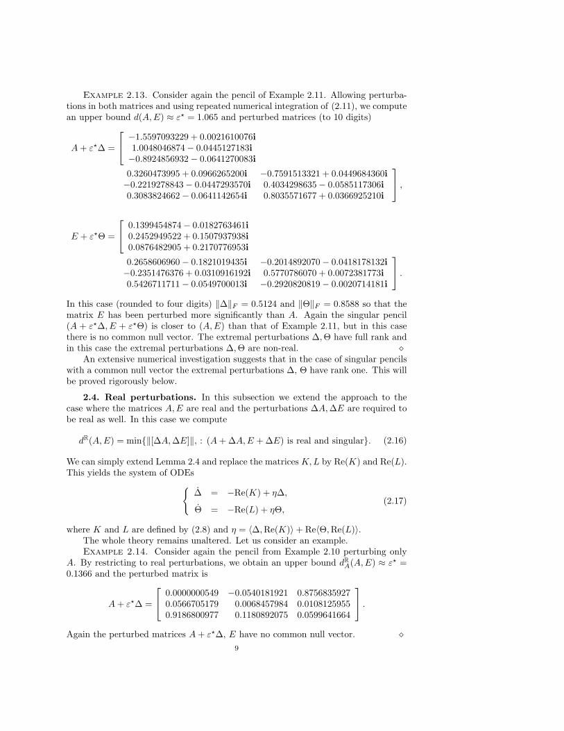
Example 2.13. Consider again the pencil of Example 2.11. Allowing perturba-tions in both matrices and using repeated numerical integration of (2.11), we computean upper bound d(A,E) ≈ ε⋆ = 1.065 and perturbed matrices (to 10 digits)
A+ ε⋆∆ =
−1.5597093229 + 0.0021610076i1.0048046874− 0.0445127183i−0.8924856932− 0.0641270083i
0.3260473995 + 0.0966265200i −0.7591513321 + 0.0449684360i−0.2219278843− 0.0447293570i 0.4034298635− 0.0585117306i0.3083824662− 0.0641142654i 0.8035571677 + 0.0366925210i
,
E + ε⋆Θ =
0.1399454874− 0.0182763461i0.2452949522 + 0.1507937938i0.0876482905 + 0.2170776953i
0.2658606960− 0.1821019435i −0.2014892070− 0.0418178132i−0.2351476376 + 0.0310916192i 0.5770786070 + 0.0072381773i0.5426711711− 0.0549700013i −0.2920820819− 0.0020714181i
.
In this case (rounded to four digits) ∥∆∥F = 0.5124 and ∥Θ∥F = 0.8588 so that thematrix E has been perturbed more significantly than A. Again the singular pencil(A + ε⋆∆, E + ε⋆Θ) is closer to (A,E) than that of Example 2.11, but in this casethere is no common null vector. The extremal perturbations ∆,Θ have full rank andin this case the extremal perturbations ∆,Θ are non-real. ⋄
An extensive numerical investigation suggests that in the case of singular pencilswith a common null vector the extremal perturbations ∆, Θ have rank one. This willbe proved rigorously below.
2.4. Real perturbations. In this subsection we extend the approach to thecase where the matrices A,E are real and the perturbations ∆A,∆E are required tobe real as well. In this case we compute
dR(A,E) = min{∥[∆A,∆E]∥, : (A+∆A,E +∆E) is real and singular}. (2.16)
We can simply extend Lemma 2.4 and replace the matrices K,L by Re(K) and Re(L).This yields the system of ODEs{
∆ = −Re(K) + η∆,
Θ = −Re(L) + ηΘ,(2.17)
where K and L are defined by (2.8) and η = ⟨∆,Re(K)⟩+Re⟨Θ,Re(L)⟩.The whole theory remains unaltered. Let us consider an example.Example 2.14. Consider again the pencil from Example 2.10 perturbing only
A. By restricting to real perturbations, we obtain an upper bound dRA(A,E) ≈ ε⋆ =0.1366 and the perturbed matrix is
A+ ε⋆∆ =
0.0000000549 −0.0540181921 0.87568359270.0566705179 0.0068457984 0.01081259550.9186800977 0.1180892075 0.0599641664
.
Again the perturbed matrices A+ ε⋆∆, E have no common null vector. ⋄9

2.5. Comparison with purely algebraic approaches. The new approach isbased on optimization methods for differential equations. The question arises whetherthe approximations obtained via this approach are superior to those obtained in apurely linear algebra fashion. In general these different approaches are hard to com-pare, since they proceed via completely different optimization methods. Except forspecial cases, see [2, 21], no proof is available that the true distance has been obtained.However, extensive numerical tests indicate that the differential equation approachachieves smaller bounds for the distance to singularity in all cases.
The easiest of the linear algebra approaches (which is not using an optimization)is to compute the generalized Schur form (UHEV,UHAV ) = (S, T ) of the pair (A,E)with upper triangular matrices S, T and then to create a pair of zero diagonal elementsin the upper triangular matrices S and T .
Example 2.15. Consider the pair (A,E) from Example 2.10. Applying the QZalgorithm, see e.g. [6], to this pair gives the generalized Schur form with
S =
0 −0.978747365727621 0.2050697298024290 0.205069729802429 0.9787473657276210 0 −0.000000000000001
,
T =
0.932148056909416 −0.102583031602284 0.0638883122982830 0.036969147238194 −0.0113263997564390 0 0.890898422941695
Considering the third diagonal element of S to be zero, we see that an upper bound forthe smallest (real and even rank-one) perturbation in T that makes the pencil singularis of size ≈ 0.8909, while the smallest perturbation in both matrices is obtainedby perturbing the second diagonal element in both S and T to zero, which is oforder 0.2084 in Frobenius norm. Both perturbations are larger than the minimalperturbations obtained by the ODE approach. ⋄
Example 2.16. Consider the following example from [2] with matrices
A = UT
1 0 00 .0001 00 0 1
V, E = UT
0 1 00 0 10 0 0
V
with real orthogonal matrices U, V . The smallest perturbation that makes the pencilsingular, perturbing both E,A or only A is real, of rank one and of size .0001.
The ODE approach correctly yields a closest singular pair at a distance approxi-mately .0001 for different choices of U and V . ⋄
Example 2.17. Consider next the following example of an 8 × 8 matrix pencilarising from the model of a two-dimensional, three-link mobile manipulator from [2,Example 14].
A =
O I3 O−K0 −D0 FT
0
F0 O O
, E =
I3 O OO M0 OO O O
,
10

with
M0 =
18.7532 −7.94493 7.94494−7.94493 31.8182 −26.81827.94494 −26.8182 26.8182
, D0 =
−1.52143 −1.55168 1.551683.22064 3.28467 −3.28467
−3.22064 −3.28467 3.28467
,
K0 =
67.4894 69.2393 −69.239369.8124 1.68624 −1.68617
−69.8123 −1.68617 −68.2707
, F0 =
[1 0 00 0 1
].
An application of the method presented in this paper gives as result the boundd(A,E) ≈ 0.011, which is consistent with the best result given in [2]. Here theclosest singular pair does not have any common left or right null vector. The modulusof Gε(∆(ε),Θ(ε)) is plotted (in logarithmic scale) in Figure 2.1. ⋄
0 0.002 0.004 0.006 0.008 0.01 0.01210
−9
10−8
10−7
10−6
10−5
10−4
10−3
ε
G ε(∆(ε),
Θ(ε))
Fig. 2.1. The function ε → Gε(∆(ε),Θ(ε)) for the illustrative example 2.17
We have seen in this section that with the ODE approach we are able to computeapproximations from above for the distance to singularity, perturbing both matricesA,E or only A and we can even deal with the real case analogously.
It cannot be guaranteed that the optimization approach reaches a global mini-mum. However, starting from different initial values, the method has the option tofind several local minima. As the examples demonstrate, the minimum may not beachieved by a perturbation where the perturbed matrices have a common null vec-tor. However, if we make it a requirement that we are only looking for a smallestperturbation with this property, then the situation changes drastically. This will bediscussed in the next section.
3. Distance to singular pencils with common null vectors: the case offixed E. In this section we consider the ODE-based approach for the minimizationproblem of finding a nearby pencil with a common right null vector. A common leftnull vector is simply obtained by applying the same procedure to the pair (AH , EH).We first discuss extensively the case that only the matrix A is perturbed and thenextend the approach to the perturbation of both matrices in the next section. In bothcases we prove that the smallest perturbations which make the pencil singular, haverank one.
11

3.1. Simple upper and lower bounds for d0A(A,E). Let us first discusspurely algebraic techniques to construct some upper and lower bounds.
The simplest lower bound is given by the distance to singularity of A, which inthe unstructured case is given by the smallest singular value σn(A). This providesthe lower bound
σn(A) ≤ d0A(A,E)
To get an upper bound for the distance to singularity we can employ the gener-alized singular value decomposition of the pair (A,E), see [6]. We have the followingLemma.
Lemma 3.1. Let A,E ∈ Cn,n with E singular and (A,E) regular. Let XAV = C,XEU = D be the generalized singular value decomposition with U, V unitary, Xinvertible, and C = diag(C1, C2), D = diag(D1, 0), diagonal, D1 invertible, and thediagonal elements of C2 are ordered in decreasing absolute value. Then the matricesA− (eTnC2en)X
−1eneTnU
H , E have a common right null vector Uen.Proof. The proof is straightforward, since by construction
X(A− (eTnC2en)X−1ene
TnU
H)Uen = 0, XEUen = 0,
which proves the result.Lemma 3.1 gives a numerically computable rank-one perturbation to A that cre-
ates a common null vector, which even is real in the real case. This clearly gives asimple upper bound for the distance to singularity. This perturbation would actuallybe minimal in Frobenius norm if the matrix X were unitary, which however is usuallynot the case. A sufficient condition for X to be unitary is that EHA = AHE andEAH = AEH , which is however, a very strong requirement.
Another upper bound can be obtained from the Jordan canonical form
A = TJT−1.
Consider any Jordan block with eigenvalue λm and replace the first diagonal elementin this block by zero (calling the resulting matrix Jm) and replace the associatedeigenvector xm in the associated column of T by its orthogonal projection onto thekernel of E leading to a matrix Tm. This projection is obtained by setting xm =xm − V2V
H2 xm, where E = UΣV H is the singular value decomposition of E and the
columns of V2 span the kernel of E. If xm is linearly independent to the remainingcolumns of T then the new pair (E, A) = (E, TmJmT−1
m ) is singular. Then, minimizing∥A− Am∥ by going through all eigenvalues of A, we obtain the upper bound
d0A(A,E) ≤ ∥A− Am∗∥,
where m∗ is the index of the eigenvalue where the bound is minimized. This upperbound is of limited practical value, since its computation requires the Jordan canonicalform which is usually not numerically computable. Using instead the ordered Schurform, see [6],
A = QSQH
with Q unitary and S upper triangular, we have that the first column of Q forms aneigenvector and we can apply the same approach of setting the eigenvalue to 0 andreplace the eigenvector by its orthogonal projection onto the kernel of E, to obtain
12

singular pencil. Using eigenvalue reordering, see [6], we can reorder the eigenvaluesone by one to the top and apply the projection in the same way and then minimize overall possible eigenvalues. This gives a numerically computable upper bound realizedby a rank-one perturbation. Usually this approach cannot be applied to obtain a realperturbation if the eigenvalues are non-real. Further bounds obtained from a purelyalgebraic approach are derived in [2].
A third upper bound is obtained from the singular value decomposition
UH
[EA
]V =
[Σ0
],
with Σ = diag(σ1, . . . , σn) and
U =
[U11 U12
U21 U22
],
with Ui,j ∈ Cn,n. Then the pencil
(A− σnU21eneTnV
H , E − σnU11eneTnV
H) (3.1)
is singular with common null vector V en, since
UH
[E − σnU11ene
TnV
H
A− σnU21eneTnV
H
]V en = 0.
This is, however, a perturbation in both matrices and it is a rank-one perturbationin each of the two.
Example 3.2. Consider the pencil from Example 2.11. In this case the pertur-bation obtained via the singular value decomposition in (3.1) is given by
∆A =
−0.0851 −0.2996 0.0397−0.0948 −0.3335 0.0442−0.0132 −0.0465 0.0062
, ∆E =
0.0000 0.0000 −0.0000−0.0343 −0.1208 0.01600.2587 0.9105 −0.1208
,
with d(A,E) = 1.0722 which is larger than the bound 1.065 obtained by the ODEapproach. ⋄
To obtain a rank-one perturbation in A only, we consider the singular valuedecomposition of E,
E = U
[Σm 00 0
]V H
with U ∈ Cn,n and V ∈ Cn,n unitary and Σm ∈ Rm,m diagonal with positive diagonalentries. (Note that in the real case the factors are real.) Partition
UHAV =
[A11 A12
A21 A22
]with A11 ∈ Cm,m accordingly, and let A22 = UAΣAV
HA be another singular value
decomposition, with ΣA = diag(ξ1, . . . , ξn−m) diagonal entries. Let
U := U
[Im
UA
], V := V
[Im
VA
]13
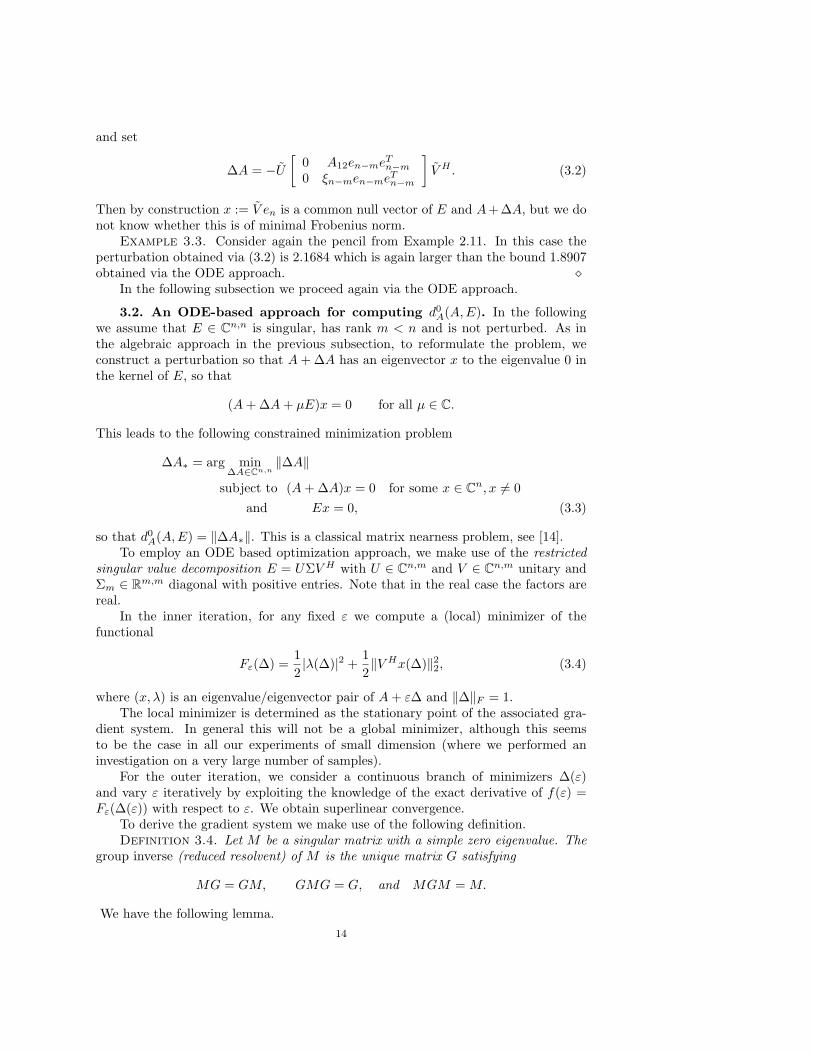
and set
∆A = −U
[0 A12en−meTn−m
0 ξn−men−meTn−m
]V H . (3.2)
Then by construction x := V en is a common null vector of E and A+∆A, but we donot know whether this is of minimal Frobenius norm.
Example 3.3. Consider again the pencil from Example 2.11. In this case theperturbation obtained via (3.2) is 2.1684 which is again larger than the bound 1.8907obtained via the ODE approach. ⋄
In the following subsection we proceed again via the ODE approach.
3.2. An ODE-based approach for computing d0A(A,E). In the followingwe assume that E ∈ Cn,n is singular, has rank m < n and is not perturbed. As inthe algebraic approach in the previous subsection, to reformulate the problem, weconstruct a perturbation so that A+∆A has an eigenvector x to the eigenvalue 0 inthe kernel of E, so that
(A+∆A+ µE)x = 0 for all µ ∈ C.
This leads to the following constrained minimization problem
∆A∗ = arg min∆A∈Cn,n
∥∆A∥
subject to (A+∆A)x = 0 for some x ∈ Cn, x = 0
and Ex = 0, (3.3)
so that d0A(A,E) = ∥∆A∗∥. This is a classical matrix nearness problem, see [14].To employ an ODE based optimization approach, we make use of the restricted
singular value decomposition E = UΣV H with U ∈ Cn,m and V ∈ Cn,m unitary andΣm ∈ Rm,m diagonal with positive entries. Note that in the real case the factors arereal.
In the inner iteration, for any fixed ε we compute a (local) minimizer of thefunctional
Fε(∆) =1
2|λ(∆)|2 + 1
2∥V Hx(∆)∥22, (3.4)
where (x, λ) is an eigenvalue/eigenvector pair of A+ ε∆ and ∥∆∥F = 1.The local minimizer is determined as the stationary point of the associated gra-
dient system. In general this will not be a global minimizer, although this seemsto be the case in all our experiments of small dimension (where we performed aninvestigation on a very large number of samples).
For the outer iteration, we consider a continuous branch of minimizers ∆(ε)and vary ε iteratively by exploiting the knowledge of the exact derivative of f(ε) =Fε(∆(ε)) with respect to ε. We obtain superlinear convergence.
To derive the gradient system we make use of the following definition.Definition 3.4. Let M be a singular matrix with a simple zero eigenvalue. The
group inverse (reduced resolvent) of M is the unique matrix G satisfying
MG = GM, GMG = G, and MGM = M.
We have the following lemma.
14

Lemma 3.5. [22, Theorem 2] Given a smooth matrix function C : R → Cn,n, letλ(t) be a simple eigenvalue of C(t) and let x(t) and y(t) be the associated right and lefteigenvectors, depending smoothly on t and normalized such that ∥x(t)∥2 = ∥y(t)∥2 = 1.
Moreover, let M(t) = C(t) − λ(t)I and let G(t) be the group inverse of M(t).Then the eigenvectors satisfy the following system of differential equations:
x(t) = x(t)x(t)HG(t)M(t)x(t)−G(t)M(t)x(t),
y(t)H = y(t)HM(t)G(t)y(t)y(t)H − y(t)HM(t)G(t) . (3.5)
In order to minimize the functional Fε(∆), we construct a family of matricesA + ε∆(t), with ∆(t) ∈ Cn,n and ∥∆(t)∥F = 1, such that limt→∞ ∆(t) = ∆∞ andan eigenvector/eigenvalue pair (x, λ) of A + ε∆∞ exists such that Fε(∆) is locallyminimized (over all matrices ∆ of unit norm).
If Fε(∆) > 0, then the derivative ∆ is chosen in the direction of steepest descentof Fε(∆) for the chosen eigenvalue/eigenvector pair of A+ ε∆.
We start by considering the first summand 12 |λ|
2 in Fε(∆) (see (3.4)), which weassume to be different from zero.
Let λ be a simple eigenvalue of A + ε∆ and let x, y be the associated right andleft eigenvectors, normalized according to (2.5). Proceeding as in (2.6) we get
1
2
d
dt|λ|2 = ε αRe⟨yxH , ∆⟩, with α =
r
|yHx|, (3.6)
so that α is well-defined by the simplicity assumption and α = 0 if λ = 0.Next we consider the second summand 1
2∥VHx∥22 in Fε(∆), which we again assume
to be different from zero. We get
1
2
d
dt∥V Hx∥22 = Re
(xHV V Hx
)= ν Re
(uHx
)(3.7)
with
u = VV Hx
∥V Hx∥2and ν = ∥V Hx∥2.
This requires the derivative of the eigenvector x of A+ ε∆(t), which is given byLemma 3.5. Inserting (3.5) into (3.7) we obtain
1
2
d
dt∥V Hx∥22 = ν Re
(uHx
)= ε ν Re
(uH((xHG∆x)x−G∆x
))+ν Re
(uH((xHGλIx)x−GλIx
)). (3.8)
Using that for a simple eigenvalue Gx = 0 and yHG = 0, see [22], we get that thesecond summand of (3.8) vanishes. Hence
1
2
d
dt∥V Hx∥22 = ε ν2 Re⟨x,G∆x⟩ − ε ν Re⟨u,G∆x⟩
= ε ν Re⟨GH(νx− u)xH , ∆⟩ = ε ν Re⟨vxH , ∆⟩,15

where v := GH(νx− u). Therefore, with w = αy + νv, we have
d
dtFε(∆) = εRe
⟨(αy + νv)xH , ∆
⟩= εRe⟨wxH , ∆⟩.
Then, the optimal steepest descent direction Z = ∆ for Fε(∆) (see (3.6) and (3.8)) isdetermined by the following optimization problem, where w is assumed to be differentfrom zero.
Z∗ = arg minZ∈Cn,n
Re⟨wxH, Z
⟩subject to Re ⟨∆, Z⟩ = 0 and ∥Z∥F = 1. (3.9)
The solution to the optimization problem (3.9) is given in the following lemma.Lemma 3.6. Let ∆ ∈ Cn,n be of unit Frobenius norm, and let w, x ∈ Cn \ {0}
be such that ∆ is not proportional to wxH . Then the solution of the optimizationproblem (3.9) is given by
κZ∗ = − wxH +Re⟨∆, wxH
⟩∆, (3.10)
where κ is the Frobenius norm of the matrix on the right hand side.Proof. The result follows by noting that the expression in (3.10) is the orthogonal
projection of the rank-one matrix wxH to the subspace {Z : Re⟨∆, Z⟩ = 0}.Lemma 3.6 suggests to consider the following gradient system for Fε(∆),
∆ = − wxH +Re⟨∆, wxH
⟩∆, (3.11)
where y(t), x(t) are left and right eigenvectors, respectively, of unit norm associatedwith a simple eigenvalue λ(t) = reiθ of A + ε∆(t) (for fixed ε), and with yHx =|yHx|e−iθ, w = αy + νv, α = |λ|/|yHx|, v = GH(νx − u), u = V V Hx/ν and ν =∥V Hx∥2.
The following result shows the monotonic decrease of Fε(∆(t)) along every solu-tion of (3.11).
Theorem 3.7. Let ∆(t) of unit Frobenius norm satisfy the differential equation(3.11). If λ(t) is a simple eigenvalue of A+ ε∆(t), then
d
dtFε (∆(t)) ≤ 0. (3.12)
Proof. The result follows directly from Lemmas 2.1, 3.5 and 3.6.The following lemma characterizes the right hand side of (3.11).Lemma 3.8. Consider the functional (3.4) and suppose that Fε(∆) > 0. Let λ
be a simple eigenvalue of A + ε∆ (for fixed ε) and let y, x be the associated left andright unit norm eigenvectors, respectively. If v = GH(νx − u), where G is the groupinverse of A+ ε∆− λI, then
w = αy + νv = 0. (3.13)
Proof. (i) First assume that λ = 0. Exploiting the well-known property of thegroup inverse that Gx = 0 [22], we obtain that xHv = 0.
16

If we had αy + νv = 0, then this would imply xH (αy + νv) = 0 and thus,αxHy = 0. Since xHy = 0 by the simplicity of λ and α = 0 by the assumption λ = 0,it follows that |αxHy| = |λ|, which is a contradiction.
(ii) Next assume that λ = 0. This implies α = 0 and ν = 0. Then w = νv withv = 1
ν
(ν2x− V V Hx
). Since λ is simple, the group inverse G of A+ ε∆−λI has rank
n− 1. This implies that ker(GH) = span(y), and hence w = 0. Therefore
ν2x− V V Hx = ηy
for some η ∈ C, η = 0. As a consequence
0 = xH(ν2x− V V Hx
)= ηxHy
which gives a contradiction, since xHy = 0.Lemma 3.8 implies that at a stationary point of (3.11) for which Fε(∆) > 0, the
summands in the right-hand side of (3.11) cannot vanish simultaneously.Stationary points of (3.11), which are potential minimizers for the computation
of Fε(∆), can be characterized as follows.Theorem 3.9. Consider the functional (3.4) and suppose that Fε(∆) > 0. Let
λ be a simple eigenvalue of A + ε∆ (for fixed ε) and let y, x be the associated leftand right unit norm eigenvectors, respectively. Then the following are equivalent onsolutions of (3.11).
(1)d
dtFε(∆) = 0;
(2) ∆ = 0;
(3) ∆ is a real multiple of wxH (where w = αy + νv).Proof. The proof follows directly by equating to zero the right hand side of (3.11)
and by Lemma 3.8, which prevents that w = 0.The following theorem characterizes the local minimizers.Theorem 3.10. Consider the functional (3.4) and suppose that Fε(∆) > 0.
Let ∆∗ ∈ Cn,n with ∥∆∗∥F = 1. Let λ∗ = reiθ be a simple eigenvalue of A + ε∆∗with left and right eigenvectors y and x, respectively, both of unit norm and with thenormalization yHx = |yHx|e−iθ and Fε(∆) > 0. Then the following are equivalent:
(i) Every differentiable path (∆(t), λ(t)) (for small t ≥ 0) such that ∥∆(t)∥F ≤ 1and λ(t) is a simple eigenvalue of A+ ε∆(t), with ∆(0) = ∆∗, satisfies
d
dtFε (∆(t)) ≥ 0.
(ii) ∆∗ is a negative multiple of wxH , where w = αy + νv.Proof. First of all note that Lemma 3.8 ensures that wxH = 0.Assume that (i) does not hold. Then there exists a path ∆(t) through ∆∗ such that
ddtF (∆(t))
∣∣t=0
< 0. The minimization property established by Lemma 3.6 togetherwith Lemmas 2.1, and 3.5 shows that also the solution path of (3.11) passing through∆∗ is such a path. Hence ∆∗ is not a stationary point of (3.11), and Theorem 3.9then yields that ∆∗ is not a real multiple of wxH . This implies that also (ii) does nothold.
Conversely, if ∆∗ is not a real multiple of wxH , then ∆∗ is not a stationary pointof (3.11), and Theorems 3.9 and 3.7 yield that d
dtF (∆(t))∣∣t=0
< 0 along the solutionpath of (3.11).
17

Moreover, using a similar argument to [9, Theorem 2.2], if
∆∗ = γwxH , with γ > 0,
then along the path ∆(t) = (1−t)∆∗, t ∈ [0, τ ] (τ > 0), which is such that ∥∆(t)∥F ≤ 1if τ ≤ 2, we have that
d
dtF (∆(t)) = −γ∥wxH∥2F < 0.
Hence, by exploiting Lemmas 2.1 and 3.5, as well as ddtF (∆(t))
∣∣t=0
< 0, this contra-dicts (i).
As a consequence, if in Theorem 3.9 we have that Fε(∆) > 0 is locally minimal,then
∆ = − w
∥w∥FxH
which is a rank-one matrix.
3.3. Rank-one property of the solution of the common null vector prob-lem with fixed E. In [21] it was conjectured that the minimal norm perturbationthat makes a pencil (A,E) singular, when only A is perturbed, is of rank one. Whilethis does not appear to be true in general (as is indicated by Example 2.10), it doeshold for the restricted case of the common nullspace problem.
Theorem 3.11. Consider a regular pencil (A,E). Then the perturbation ∆A ofminimal Frobenius norm such that A+∆A and E have a common null vector, is suchthat ∆A has rank one.
Proof. The result is a consequence of the rank-one property of extremizers. Infact, we have shown above that for any ε such that Fε(∆(ε)) > 0 for ε < ε⋆ andFε(∆(ε⋆)) = 0, the extremizers ∆(ε) of Fε(∆) have rank one. They converge to arank-one matrix as ε → ε⋆ by the lower semi-continuity of the rank.
Since for a rank-one matrix the Frobenius norm and the matrix 2-norm are thesame, Theorem 3.11 further shows that there is a perturbation ∆A of minimal 2-normsuch that A+∆A and E have a common null vector, which has rank one. There may,however, be further perturbations of the same 2-norm that have arbitrary rank.
3.4. Rank-one dynamics to compute the distance to singularity withcommon null space. Since the extremizers of (3.4) are of rank one, we can proceedin complete analogy to [8] to obtain a suitable ODE on the manifold M1 of rank-onematrices in Cn,n.
We express ∆ ∈ M1 as ∆ = σpqH , where σ ∈ C, p, q ∈ Cn have unit norm, andthe derivatives σ ∈ C, p, q ∈ Cn will be uniquely determined from σ, p, q and ∆ byimposing the orthogonality conditions pH p = 0, qH q = 0.
In the differential equation (3.11) we replace the right-hand side by its orthogonalprojection to the tangent space T∆M1 of the manifold M1 and obtain
∆ = P∆
(−wxH +Re⟨∆, wxH⟩∆
), (3.14)
where x and y are again unit norm right and left eigenvectors, respectively, associatedwith a simple eigenvalue λ of A + ε∆, with yHx > 0 and w = αy + νv, where α, νand v are defined as before.
18

The orthogonal projection onto T∆M1 at ∆ = σpqH ∈ M1 is given by
P∆(Z) = Z − (I− ppH)Z(I− qqH) (3.15)
for some Z ∈ Cn,n. With this formula we immediately obtain the following lemma.Lemma 3.12. Consider the orthogonal projection P∆(Z) as in (3.15). For ∆ =
σpqH ∈ M1 with nonzero σ ∈ C and with p ∈ Cn and q ∈ Cn of unit norm, theequation ∆ = P∆(Z) is equivalent to ∆ = σpqH + σpqH + σpqH , where
σ = pHZq,
p = (I − ppH)Zqσ−1,
q = (I − qqH)ZHpσ−1. (3.16)
Proof. The proof follows by using the rank-one representation of ∆; see [8].Inserting Z = −wxH+Re⟨∆, wxH⟩∆, we get that the differential equation (3.14)
for ∆ = σpqH can be rewritten as the following system of differential equations forσ, p and q. Here we set η = − pHw ∈ C, β = qHx ∈ C.
σ = ηβ − Re(ηβσ)σ = i Im(ηβσ)σ,
p = (−w − ηp)βσ−1,
q = (x− βq)η σ−1. (3.17)
The derivation of this system of ODEs is straightforward; see [9] for the details.A nice consequence of this reformulation of the gradient system is that the mono-
tonicity and the characterization of stationary points is analogous to those obtainedfor (3.11), i.e., we have Theorems 3.7 and 3.9 (for the proofs we refer to [8]). Thismeans that the rank-one ODE has the same stationary points as (3.11), which includethe desired extremizers.
As a consequence we can integrate the ODE (3.17) instead of (3.11) in the in-ner iteration of the optimization procedure. Based on this, we present in the nextsubsection a corresponding numerical method for the outer iteration.
3.5. The outer iteration, updating ε. In this subsection we discuss the outeriteration to update ε. For every ε > 0, the gradient system (3.11) yields a sta-tionary point ∆(ε) of unit Frobenius norm that is a (local) minimum of Fε. Themethod is constructed to approach, from the left-hand side, the value ε⋆ > 0 suchthat Fε⋆(∆(ε⋆)) = 0 and Fε(∆(ε)) > 0 for ε < ε⋆. We make the following genericassumption.
Assumption 3.13. The smallest eigenvalue λ(ε) of the extremal matrix A+ε∆(ε)is simple. Moreover, we assume that ∆(ε) and λ(ε), x(ε) are smooth with respect to ε(at least in a neighborhood of ε⋆).
The following result provides an explicit and easily computable expression for thederivative of Fε(∆(ε)) with respect to ε.
Theorem 3.14. Consider the optimization problem of determining a rank-oneperturbation minimizing Fε(∆(ε)) by perturbing only A. Suppose that:
1. ε ∈ (0, ε⋆) such that Fε(∆(ε)) > 0,2. Assumption 3.13 holds.
Then,
dFε(∆(ε))
dε= −
∥∥∥w(ε)x(ε)H∥∥∥F< 0, for all ε,
19

where
w(ε) = α(ε)y(ε) + ν(ε)v(ε), α(ε) =|λ(ε)|
|y(ε)Hx(ε)|, v(ε) = G(ε)H
(ν(ε)x(ε)− u(ε)
),
and
u(ε) = VV Hx(ε)
∥V Hx(ε)∥, ν(ε) = ∥V Hx(ε)∥2.
Proof. The proof is similar to that of Theorem 2.9.
Having obtained a computational method to compute the minimal rank-one per-turbation of A which makes the pencil (A,E) singular, we prove below that actuallythis gives the solution to the general rank perturbation.
3.6. Numerical examples for the common nullspace problem with fixed E.In this subsection we present several illustrative numerical examples.
Example 3.15. Consider the pencil from Example 2.11. Running the algorithmpresented in the last subsection to the pair (AH , EH) we obtain the same distanceε⋆ ≈ 1.8907 as computed by means of the general algorithm, with the rank-oneperturbation to be added to A given by ∆ = σqpH with
σ = 0.9987− 0.0506i,
p =[−0.8277− 0.4597i 0.0462 + 0.0257i −0.2775− 0.1541i
]T,
q =[−0.8975− 0.4406i −0.0066− 0.0010i 0.0132 + 0.0117i
].
⋄Example 3.16. Consider the matrices
A =
0.49 0.89 0.33 0.32 1.09 −0.011.03 −1.15 −0.75 0.31 1.11 1.530.73 −1.07 1.37 −0.86 −0.86 −0.77
−0.30 −0.81 −1.71 −0.03 0.08 0.370.29 −2.94 −0.10 −0.16 −1.21 −0.23
−0.79 1.44 −0.24 0.63 −1.11 1.12
, E =
0 0 0 0 1 00 1 0 1 0 00 1 0 1 0 01 0 0 0 1 11 1 0 0 0 11 0 0 0 0 1
.
The matrix E has rank 4 and an orthonormal basis for ker(E)⊥ is given by
V =
0.6196 −0.2399 −0.1986 −0.13840.3846 0.6684 −0.0501 0.63470.0000 0.0000 0.0000 −0.00000.1532 0.6229 0.2343 −0.73040.2469 −0.2236 0.9294 0.15920.6196 −0.2399 −0.1986 −0.1384
.
The simple bounds
0.1936 ≤ d0A(A,E) ≤ 7.2810
are computed according to the procedure given in Subsection 3.1.
20

Applying the ODE-based approach, we obtain ε⋆ ≈ 1.21 and the correspondingmatrix ∆ is given by
∆∗ = pxH , x ≈
−0.5740.0000.5830.0000.0000.574
, p ≈
−0.075 + 0.134i−0.125− 0.029i−0.052 + 0.065i−0.498 + 0.096i−0.295 + 0.021i0.779 + 0.041i
.
The monotonicity of the functional Fε in ε = ε⋆ is shown in Figure 3.1. ⋄
0 200 400 600 800 100010−14
10−12
10−10
10−8
10−6
10−4
10−2
10 0
Fig. 3.1. The function t → Fε⋆ (∆(t)) for Example 3.16.
Example 3.17. Consider, see [6],
Bn =
1 −1 −1 · · · −1
1 −1 · · · −1. . .
......
1 −11
.
This is an ill-conditioned triangular matrix with no small diagonal entry. The rank-one perturbation ∆B = −22−nene
T1 makes Bn singular.
Thus for the pencil (A,E) = (Bn, Bn +∆B) if we perturb A by ∆B leads to thedistance to singularity d0A(A,E) ≤ 22−n.
In the general case the null vector of E is
x =[2n−2 2n−1 . . . 2 1 1
]Tand we can look for
∆A =
0 0 . . . 0 00 0 . . . 0 00 0 . . . 0 0δn δn−1 . . . δ2 δ1
,
21

such that (δ + e1)T x = 0, where
δ = [δn δn−1 . . . δ3 δ2 δ1]T
and ∥δ∥F is minimal. The minimization problem
minδ1,...,δn
n∑i=1
δ2i s.t.n∑
i=1
δixi = −1
is easily solvable and the solution is
δ = − x/∥x∥2 such that ∥∆A∥F =1
∥x∥.
Note that imposing a left common null vector would lead to the same distance andthe optimal perturbation would have the first column equal to the last row of ∆A inreverse order.
Consider for example the case n = 5, where d0A(A,E) ≤ 1/8 = 0.125. The exactclosest singular pair is obtained with the perturbation
∆A = −
0 0 0 0 00 0 0 0 00 0 0 0 00 0 0 0 0443
243
143
122
186
,
having (up to four digits) the Frobenius norm ∥∆A∥F = 1√86
= 0.107833.
The ODE method correctly finds an accurate approximation of ∆A also for largervalues of n. For example, for n = 10, it correctly approximates the distance and theoptimal perturbation to six digits.
Finally, according to our experiments, dA(A,E) < d0A(A,E). For example, forn = 10, we obtain d(A,E) ≈ 0.0030, dA(A,E) ≈ 0.030 and d0A(A,E) ≈ 0.034. ⋄
3.7. Numerical integration of the gradient system. For the numerical in-tegration of the gradient system (3.17) we apply a suitable variable stepsize projectedEuler method, in order to preserve the norm of p and q and the modulus 1 propertyof σ. In order to control the stepsize, we simply require the monotonicity propertyof the exact flow, i.e., F (∆(tℓ+1)) < F (∆(tℓ)). For this reason we do not estimate∥∆(tℓ+1)−∆ℓ+1∥ as we do not make use of any classical error estimate on the solution.
Concerning the outer iteration, by definition, the function Fε(∆(ε)) has generi-cally a double zero at ε = ε⋆ and then vanishes identically for ε > ε⋆. This suggests toapproach the root from the left, while values ε > ε⋆ may only provide upper bounds.
Let f(ε) = Fε(∆(ε)). Since for ε < ε⋆ we can exploit the knowledge of f(ε) aswell as f ′(ε). Similarly to the case discussed in Section 2.2, for εk < ε⋆ we can set
εk+1 = εk − 2f(εk)
f ′(εk)
and obtain a quadratically convergent iteration from the left.At every step of the outer iteration we need to compute the smallest eigenvalue and
the associated eigenvectors of the matrix A+ε∆n. For small dense problems we use theQR algorithm implemented in eig, while for problems of large dimension (and possibly
22

sparse structure) we make use of the routine eigs, which is based on ARPACK [19]and implements the implicitly restarted Arnoldi method. A major computationalproblem when computing the right-hand side of the differential equations (3.11) and(3.17) is the the application of the group inverse G to a vector. In order to computeit efficiently we make use of the following result from [11].
Theorem 3.18. Suppose that the matrix B has a semisimple eigenvalue 0 withx ∈ ker(B) and y ∈ ker(BH) of unit norm and such that yHx > 0. Let G be the groupinverse of B. Then
G = ΠB†Π = Π(B + ηyxH
)−1Π , (3.18)
where η ∈ R, B† is the Moore-Penrose pseudoinverse of B, Π is the projection(I − ηxyH
), with y = y/(yHx) and η = 0 is arbitrary.
In our case we apply Theorem 3.18 with B = A − λI + ε∆, so that G =Π(A− λI + εΓ)
−1Π, where
Γ = gxH , g = −w + y
is a rank-one matrix. Hence we can make use of the Sherman-Morrison-Woodburyformula, see [6], so that with L = (A− λI)
−1, we obtain
(A− λI + εΓ)−1
= L− 1
(1 + εxHLγ)LγxHL.
This allows for an efficient computation of the application of G to a vector. Note alsothat G is well-conditioned if λ is not close to another eigenvalue.
We usually observe that the term |λ(∆)|2 is more rapidly converging to zerothan the term ∥V Hx(∆)∥22. This leads to an oscillating behavior close to zero of thefirst term, which causes a stepsize restriction and a consequent slowing down of theconvergence close to the stationary point, see Figure 3.2.
3 4 5 6 7 8 9 10 110
0.05
0.1
0.15
0.2
0.25
0.3
0.35
Fig. 3.2. Zoom of the two terms |λ|2 (in red) and ∥V Hx∥22 (in blue) and the functional F (inblack) versus time for the illustrative example of Section 3.6 (with ε = 1)
In this section we have obtained convincing results and a quadratically convergentmethod to compute the distance to a singular pencil with common null vector, whereonly one of the matrices is perturbed. In the next section we consider again thecommon null vector problem but allow perturbations in both matrices.
23

4. Distance to singular pencils with common null vectors. We now studythe distance to a pencil with common null vector when both matrices A and E areperturbed.
4.1. An ODE-based approach for computing d0(A,E). We look for theclosest pair of matrices (A + ∆A,E + ∆E) so that A + ∆A is singular with aneigenvector x to the eigenvalue zero belonging to ker(E+∆E). In this way we wouldget
(A+∆A+ µ(E +∆E))x = 0 for all µ ∈ C.
This problem can be reformulated as
(∆A∗,∆E∗) = arg min∆A,∆E∈Cn,n
∥(∆A,∆E)∥
subject to (A+∆A)x = 0
and (E +∆E)x = 0 for some x ∈ Cn, x = 0. (4.1)
We then have d0(A,E) = ∥(∆A∗,∆E∗)∥.In the inner iteration for the perturbation size ε we consider the perturbed matri-
ces A+ ε∆ and E + εΘ with ∥(∆,Θ)∥F = 1. Let us denote by (λ, x, y) an eigentripleof A+ ε∆ (with λ to be driven to zero) and by (ν, a, b) an eigentriple of E+ εΘ (withν to be driven to zero), where the eigenvectors are scaled according to (2.5).
The functional we aim to minimize in order to compute the closest pair with acommon right null vector is given by
Fε(∆,Θ) =1
2
(∥λ∥22 + ∥ν∥22 + (1− |xHa|2)
). (4.2)
This is phase-invariant with respect to the eigenvectors x and a, which we assume tobe normalized such that ∥x∥ = ∥a∥ = 1.
Similarly, for computing the closest pair with a common left null vector, we simplyreplace (A,E) by (AH , EH), x by y and a by b. The computation of the gradient isobtained similarly to previous cases, and we obtain the expressions
1
2
d
dt|λ|2 = α εRe⟨yxH , ∆⟩, with α =
|λ||yHx|
,
1
2
d
dt|ν|2 = β εRe⟨baH , Θ⟩, with β =
|ν||bHa|
as before. The other term instead, is given by
1
2
d
dt
(|xHa|2
)=
1
2
d
dt
(xHaaHx
)= Re
(xHaaH x
)+Re
(aHxxH a)
). (4.3)
This yields
1
2
d
dt
(|xHa|2
)= εRe
(|xHa|2xHG∆x− (xHa)aHG∆x
)+ εRe
(|xHa|2aHNΘa− (aHx)xHNΘa
)= εRe
(⟨|θ|2 GHxxH − θGHaxH , ∆
⟩+⟨|θ|2 NHaaH − θNHxaH , Θ
⟩),
24
where θ = xHa, G is the group inverse of A+ ε∆− λI, and N is the group inverse ofE + εΘ− νI.
In order to minimize the gradient of F we collect the summands involving ∆ andthose involving Θ. We get
d
dtFε(∆,Θ) = εRe⟨(αy − v) xH , ∆⟩+ εRe⟨(βb− w) aH , Θ⟩,
with v = |θ|2 GHx− θGHa and w = |θ|2 NHa− θNHx.
This leads to the system of ODEs,
∆ = − (αy − v) xH + η∆,
Θ = − (βb− w) aH + ηΘ, (4.4)
where
η = Re⟨∆, (αy − v)xH⟩+Re⟨Θ, (βb− w) aH⟩
ensures the norm conservation.
We obtain similar results to those given for the case of fixed E. In particular wehave the following result which characterizes the right hand side of (4.4).
Lemma 4.1. Let Fε(∆,Θ) > 0; let λ be a simple eigenvalue of A+ε∆ (ε is fixed)and let y, x be the left and right associate eigenvectors scaled according to (2.5). Let νbe a simple eigenvalue of E+εΘ and let b, a be the left and right associate eigenvectorsscaled according to (2.5). If θ = xHa = 0, then
αy − v = 0 and βb− w = 0. (4.5)
Proof. We prove that u1 = αy − v cannot vanish, the proof for u2 = βb− w usesthe same arguments. (i) First assume that λ = 0. Exploiting the property Gx = 0,[22], we obtain that xHv = 0. Then, assume by contradiction that u1 = 0. Thiswould imply xH (αy − v) = 0 and hence αxHy = 0. Since xHy = 0 by the simplicityof λ, and since α = 0 by the assumption λ = 0, it follows that |αxHy| = |λ|, whichgives a contradiction.
(ii) If λ = 0 then α = 0 and u1 = v with v = |θ|2 GHx− θGHa. By the simplicityassumption on λ, the group inverse G of A + ε∆ has rank n − 1. This implies thatker(GH) = Span(y). Hence, u1 = 0 implies that |θ|2 x−θ a = ηy for some η ∈ C, η = 0.As a consequence 0 = xH(|θ|2 x−θ a) = ηxHy which is a contradiction, since xHy = 0.
4.2. Rank-one property of the common nullspace problem. In the sameway as in Section 3.3, we obtain from (4.4) and Lemma 4.1 the following property.
Theorem 4.2. Consider a regular pencil (A,E). Then the perturbation of mini-mal Frobenius norm (∆A,∆E) such that A+∆A and E +∆E have a common nullvector, is such that ∆A and ∆E each have rank at most one.
4.3. Numerical examples. We consider here the same matrices of Section 3.6.
Consider first Example 2.11. Applying the ODE method leads to the bound (toseven digits) d0(A,E) ≤ 0.9438619, which is about the half of d0A(A,E). The closest
25

computed singular pencil (with a left common null vector) is
A+ ε∆ ≈
−1.6212384085 0.3554202002 −0.51308861351.0469394294 −0.2266297260 0.5965969015
−0.9441526182 0.2179904923 0.7121049288
,
E + εΘ ≈
−0.0000071285 0.1271034578 −0.48443211650.0000052330 0.1505583462 0.4262604190
−0.0000023335 0.9605965130 0.1501681259
.
Note that the first column of E + εΘ, which should be 0 analytically, vanishes withinthe stopping tolerance of the method (10−6). The rank-one matrices ∆ and Θ havenorms: ∥∆∥F ≈ 0.544470 and ∥Θ∥F ≈ 0.838781.
Consider next Example 3.17 in Section 3.6. Applying the ODE method for thecase n = 5 leads to the bound (up to seven digits) d0(A,E) ≤ 0.100177, which isslightly smaller than d0A(A,E) = 0.107833. The associated computed nearby singularpencil (having a common right null vector) is
A+ ε∆ ≈0.9976840743 −1.0009737845 −1.0004216057 −1.0002259729 −0.9997389967
−0.0043828536 0.9981784774 −1.0007637414 −1.0003813706 −0.9996427155−0.0090482003 −0.0038535312 0.9983442615 −1.0008191138 −0.9995477484−0.0192177591 −0.0083685364 −0.0036814287 0.9981783278 −0.9994870221−0.0832976242 −0.0387575470 −0.0183979414 −0.0095660488 0.9986398210
,
E + εΘ ≈0.9978049925 −1.0010539505 −1.0005015794 −1.0002252097 −1.0002971485
−0.0041176936 0.9979859780 −1.0009837884 −1.0004756378 −1.0005660223−0.0085861355 −0.0041836454 0.9979713164 −1.0009608668 −1.0012320110−0.0184060466 −0.0089312241 −0.0042987506 0.9980091457 −1.0027097718−0.1086298824 −0.0003050093 −0.0000845822 0.0000456939 0.9998338096
.
Note that ∥∆∥F ≈ 0.9709 and ∥Θ∥F ≈ 0.2395.For n = 10 we find instead d0(A,E) ≤ 0.00320, slightly larger than the computed
bound for d(A,E).
5. Conclusions and further work. We have investigated the distance of agiven regular pencil to a singular one. For the closest singular pencil we have consid-ered two cases, one where the pencil is singular due to a common left or right nullvector and the general situation where such a situation need not occur. For the firstcase we have proved that the distance can always be determined by rank-one pertur-bations both in A and in E. For the second case we expect instead that in generalthe perturbations have full rank.
We have presented and analyzed algorithms based on an inner-outer iteration,where ordinary differential equations are driven into a stationary state in the inneriteration and the outer iteration solves for a scalar distance parameter. The algorithmsfor computing the closest pencil with a common null vector can exploit the low-rankstructure of the perturbations such that the computational work grows only linearlywith the dimension in the case of a sparse pencil, which makes the algorithms fastalso for large sparse problems.
Possible future work is related to the analysis of problems with structure. A verybrief discussion of some cases of interest is given in the following:
26

• Real pencils: As we have noted in Section 2.4, in the case of real pencilsand real perturbations it is sufficient to replace the vector fields by their realparts, i.e., with their projection on the space of real matrices.
• Hermitian pencils: Similarly, for Hermitian pairs it is sufficient to choose thevalues µi ∈ R to guarantee that the solution of (2.11) remains Hermitian (forHermitian initial values). The same holds for equations (3.11), (4.4).
• Sparse pencils: In the case where A and E have a prescribed sparsity patternwhich has to be inherited also by the considered perturbations, we have toreplace the vector fields in the ODEs by their orthogonal projections on thesparsity pattern structure, which is simply obtained by annihilating thoseentries which correspond to zero entries in the sparsity patterns of A,E.
Acknowledgments. The authors thank Daniel Kressner for his helpful remarks.
The first author thanks the Italian M.I.U.R. and the INdAM GNCS for financialsupport and also the Center of Excellence DEWS.
The research of the third author was carried out in the framework of Math-eon project D-SE1, Stability analysis of power networks and power network modelssupported by Einstein Foundation Berlin.
REFERENCES
[1] K. E. Brenan, S. L. Campbell, and L. R. Petzold. Numerical Solution of Initial-Value Problemsin Differential Algebraic Equations. SIAM Publications, Philadelphia, PA, 2nd edition,1996.
[2] R. Byers, C. He, and V. Mehrmann. Where is the nearest non-regular pencil. Linear AlgebraAppl., 285:81–105, 1998.
[3] S. L. Campbell. Linearization of DAE’s along trajectories. Z. Angew. Math. Phys., 46:70–84,1995.
[4] E. Eich-Soellner and C. Fuhrer. Numerical Methods in Multibody Systems. B. G. TeubnerStuttgart, 1998.
[5] F. R. Gantmacher. Theory of Matrices. Chelsea, New York, 1959.[6] G. H. Golub and C. F. Van Loan. Matrix Computations. Johns Hopkins University Press,
Baltimore, 3rd edition, 1996.[7] N. Guglielmi, D. Kressner, and C. Lubich. Low rank differential equations for hamiltonian
matrix nearness problems. Numer. Math., 129:279–319, 2015.[8] N. Guglielmi and C. Lubich. Differential equations for roaming pseudospectra: paths to ex-
tremal points and boundary tracking. SIAM J. Numer. Anal., 49:1194–1209, 2011.[9] N. Guglielmi and C. Lubich. Low-rank dynamics for computing extremal points of real pseu-
dospectra. SIAM J. Matrix Anal. Appl., 34:40–66, 2013.[10] N. Guglielmi and M. Overton. Fast algorithms for the approximation of the pseudospectral
abscissa and pseudospectral radius of a matrix. SIAM J. Matrix Anal. Appl., 32:1166–1192,2011.
[11] N. Guglielmi, M. Overton, and G. Stewart. An efficient algorithm for computing the generalizednull space decomposition. SIAM J. Matrix Anal. Appl., 36:38–54, 2015.
[12] E. Hairer, C. Lubich, and M. Roche. The Numerical Solution of Differential-Algebraic Systemsby Runge-Kutta Methods. Springer-Verlag, Berlin, Germany, 1989.
[13] E. Hairer and G. Wanner. Solving Ordinary Differential Equations II: Stiff and Differential-Algebraic Problems. Springer-Verlag, Berlin, Germany, 2nd edition, 1996.
[14] N. J. Higham. Matrix nearness problems and applications. In M. Gover and S. Barnett, editors,Applications of Matrix Theory, pages 1–27. Oxford University Press, 1989.
[15] T. Kato. Perturbation Theory for Linear Operators. Springer Verlag, New York, N.Y., 1995.[16] Daniel Kressner and Matthias Voigt. Distance problems for linear dynamical systems. In
Numerical algebra, matrix theory, differential-algebraic equations and control theory, pages559–583. Springer, Cham, 2015.
[17] P. Kunkel and V. Mehrmann. Differential-Algebraic Equations. Analysis and Numerical Solu-tion. EMS Publishing House, Zurich, Switzerland, 2006.
27

[18] R. Lamour, R. Marz, and C. Tischendorf. Differential-Algebraic Equations: A Projector BasedAnalysis. Differential-Algebraic Equations Forum. Springer Verlag, 2013.
[19] R. B. Lehoucq, D. C. Sorensen, and C. Yang. ARPACK Users’ Guide: Solution of Large-ScaleEigenvalue Problems with Implicitly Restarted Arnoldi Methods. SIAM, Philadelphia, 1998.
[20] The MathWorks, Inc., Natick, MA. 2013. http://www.mathworks.de/products/simscape/.[21] C. Mehl, V. Mehrmann, and M. Wojtylak. On the distance to singularity via low rank pertur-
bations. Operators and Matrices, 9:733–772, 2015.[22] C.D. Meyer and G.W. Stewart. Derivatives and perturbations of eigenvectors. SIAM J. Numer.
Anal., 25:679–691, 1988.[23] Modelica Association. Modelica standard library 3.2.1. https://www.modelica.org/.[24] R. Riaza. Differential-algebraic systems. Analytical aspects and circuit applications. World
Scientific Publishing Co. Pte. Ltd., Hackensack, NJ., 2008.
28