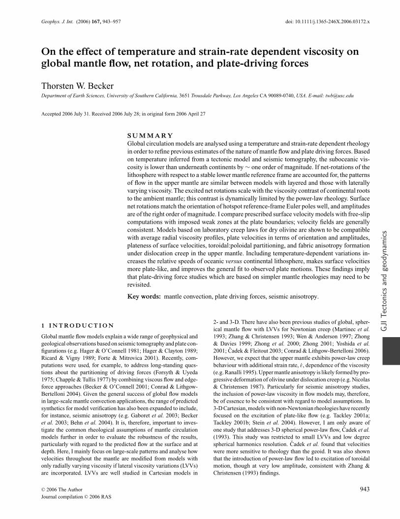
Geophys. J. Int. (2006) 167, 943–957 doi: 10.1111/j.1365-246X.2006.03172.x

GJI

Tec

toni

csan

dge

ody

nam

ics

On the effect of temperature and strain-rate dependent viscosity onglobal mantle flow, net rotation, and plate-driving forces

Thorsten W. BeckerDepartment of Earth Sciences, University of Southern California, 3651 Trousdale Parkway, Los Angeles CA 90089-0740, USA. E-mail: twb@usc.edu

Accepted 2006 July 31. Received 2006 July 28; in original form 2006 April 27

S U M M A R YGlobal circulation models are analysed using a temperature and strain-rate dependent rheologyin order to refine previous estimates of the nature of mantle flow and plate driving forces. Basedon temperature inferred from a tectonic model and seismic tomography, the suboceanic vis-cosity is lower than underneath continents by ∼ one order of magnitude. If net-rotations of thelithosphere with respect to a stable lower mantle reference frame are accounted for, the patternsof flow in the upper mantle are similar between models with layered and those with laterallyvarying viscosity. The excited net rotations scale with the viscosity contrast of continental rootsto the ambient mantle; this contrast is dynamically limited by the power-law rheology. Surfacenet rotations match the orientation of hotspot reference-frame Euler poles well, and amplitudesare of the right order of magnitude. I compare prescribed surface velocity models with free-slipcomputations with imposed weak zones at the plate boundaries; velocity fields are generallyconsistent. Models based on laboratory creep laws for dry olivine are shown to be compatiblewith average radial viscosity profiles, plate velocities in terms of orientation and amplitudes,plateness of surface velocities, toroidal:poloidal partitioning, and fabric anisotropy formationunder dislocation creep in the upper mantle. Including temperature-dependent variations in-creases the relative speeds of oceanic versus continental lithosphere, makes surface velocitiesmore plate-like, and improves the general fit to observed plate motions. These findings implythat plate-driving force studies which are based on simpler mantle rheologies may need to berevisited.

Key words: mantle convection, plate driving forces, seismic anisotropy.

1 I N T RO D U C T I O N

Global mantle flow models explain a wide range of geophysical and

geological observations based on seismic tomography and plate con-

figurations (e.g. Hager & O’Connell 1981; Hager & Clayton 1989;

Ricard & Vigny 1989; Forte & Mitrovica 2001). Recently, com-

putations were used, for example, to address long-standing ques-

tions about the partitioning of driving forces (Forsyth & Uyeda

1975; Chapple & Tullis 1977) by combining viscous flow and edge-

force approaches (Becker & O’Connell 2001; Conrad & Lithgow-

Bertelloni 2004). Given the general success of global flow models

in large-scale mantle convection applications, the range of predicted

synthetics for model verification has also been expanded to include,

for instance, seismic anisotropy (e.g. Gaboret et al. 2003; Becker

et al. 2003; Behn et al. 2004). It is, therefore, important to inves-

tigate the common rheological assumptions of mantle circulation

models further in order to evaluate the robustness of the results,

particularly with regard to the predicted flow at the surface and at

depth. Here, I mainly focus on large-scale patterns and analyse how

velocities throughout the mantle are modified from models with

only radially varying viscosity if lateral viscosity variations (LVVs)

are incorporated. LVVs are well studied in Cartesian models in

2- and 3-D. There have also been previous studies of global, spher-

ical mantle flow with LVVs for Newtonian creep (Martinec et al.1993; Zhang & Christensen 1993; Wen & Anderson 1997; Zhong

& Davies 1999; Zhong et al. 2000; Zhong 2001; Yoshida et al.2001; Cadek & Fleitout 2003; Conrad & Lithgow-Bertelloni 2006).

However, we expect that the upper mantle exhibits power-law creep

behaviour with additional strain rate, ε, dependence of the viscosity

(e.g. Ranalli 1995). Upper mantle anisotropy is likely formed by pro-

gressive deformation of olivine under dislocation creep (e.g. Nicolas

& Christensen 1987). Particularly for seismic anisotropy studies,

the inclusion of power-law viscosity in flow models may, therefore,

be of essence to be consistent with regard to model assumptions. In

3-D Cartesian, models with non-Newtonian rheologies have recently

focused on the excitation of plate-like flow (e.g. Tackley 2001a;

Tackley 2001b; Stein et al. 2004). However, I am only aware of

one study that addresses 3-D spherical power-law flow, Cadek et al.(1993). This study was restricted to small LVVs and low degree

spherical harmonics resolution. Cadek et al. found that velocities

were more sensitive to rheology than the geoid. It was also shown

that the introduction of power-law flow led to excitation of toroidal

motion, though at very low amplitude, consistent with Zhang &

Christensen (1993) findings.

C© 2006 The Author 943Journal compilation C© 2006 RAS

944 T. W. Becker

Since a comprehensive study on the role of rheology for mantle

flow in the present-day plate-tectonic setting at higher resolution

is still missing, I analyse global, temperature-dependent, power-

law flow models, building on Becker et al. (2006b), Becker et al.(2006a). We found that variations in large-scale flow fields due to the

rheological assumptions are on average less important than other un-

certainties such as the inferred density structures. In a related study,

Conrad & Lithgow-Bertelloni (2006) recently analysed the effect

of temperature-dependent viscosity on the viscous tractions that are

exerted on the lithosphere by mantle flow. These authors found that

the directions of shear vary little as a function of viscosity varia-

tions, but the drag amplitudes increase with the relative viscosity

contrast of strong subcontinental roots. The present study follows

up on Zhong (2001) (hereafter: ZH01), Cadek & Fleitout (2003)

and Conrad & Lithgow-Bertelloni (2006) work, and is in essence

an abridged, spherical version of the seminal study by Christensen

(1984). He found that 2-D convection with temperature and strain-

rate dependent viscosity is similar to Newtonian flow for certain

conditions. Substantiating earlier 2-D and 3-D work, I show that

the effect of power-law induced variations is indeed moderate in

terms of changing the patterns of global mantle flow. This is partic-

ularly the case for the uppermost mantle, which is presumably most

important for studies of seismic anisotropy. I study both models

with prescribed plate motions, and ‘self-consistent’ models with a

free-slip mechanical boundary condition on top and imposed weak

zones along plate boundaries. ‘Self-consistent’ here means force-

equilibrium for the entirely density-driven free-slip models, not a

consistent generation of plates and plate boundaries, which I do not

attempt here (see e.g. Bercovici et al. 2000, for a discussion). As

LVVs can potentially excite net motion of the mantle, the proper

reference frame becomes an issue. However, if mean rotations are

corrected for, the results are consistent for both approaches.

My results lend confidence in the gross conclusions of earlier

work using global flow models. In terms of the fit to observed plate

motions, models with LVVs due to temperature-dependent creep are

more Earth-like. While LVVs do modify the flow, especially with

regard to amplitudes, the flow geometry effects are probably most

important for regional, or higher-resolution applications.

2 M E T H O D S

2.1 Model set-up

Mantle convection is approximated by solving the equations for

instantaneous, incompressible, infinite Prandtl number, fluid flow

(e.g. Zhong et al. 2000). Following Conrad & Lithgow-Bertelloni

(2006), internal density and rheological anomalies are inferred based

on a combination of seismic tomography, seafloor age and a tectonic

model. The idea is to study the effect of LVVs for a generic set-up

that purposefully does not account for details, such as shallow struc-

ture within oceanic plates (e.g. Ritzwoller et al. 2004). Underneath

oceanic regions in the upper boundary layer, Muller et al. (1997)

and the 3SMAC (Nataf & Ricard 1996) interpolation are used for

seafloor ages, t, to assign a half-space cooling profile with non-

dimensional temperature T (t, z) = erf(z/(2√

κt)). Here, z is depth,

and κ thermal diffusivity (see Table 1 for model parameters). The

maximum oceanic plate ‘thickness’ (depth where T = 0.95) is lim-

ited to 100 km. Underneath continents, the lithospheric thickness

is estimated by finding the depth up to which seismic tomography

consistently shows a fast shear wave, vS , anomaly of d ln vS = 2

per cent. I mostly use the composite model smean of Becker &

Boschi (2002) as a reference for velocity anomalies of the mantle.

Table 1. Dynamic model parameters. The Rayleigh number is defined using

the Earth’s radius as in Zhong et al. (2000).

Parameter Symbol Value

Density/velocity anomaly D = d ln ρd ln vS

0.15

Scaling

Thermal diffusivity κ 10−6 m2 s−1

Thermal expansivity α 2 · 10−5 K−1

Scaling temperature difference �T 1785◦ K

Non-dimensional temperature TNon-dimensional reference Tc 1

(background) temperature

Non-dimensional temperature dTd ln vS

= − Dα�T −4.2

Anomaly scaling, T = Tc + dTGravitational acceleration g 10 m s−2

Reference density ρ 3300 kg m−3

Reference viscosity η0 2 × 1021 Pa s

Earth’s radius R 6371 km

Rayleigh number Ra = gαρ�T R3

κη01.5 · 108

Half-space cooling profiles with pseudo-ages are then fit (Conrad

& Lithgow-Bertelloni 2006), roughly matching these depths up to

a maximum thickness of 300 km.

Above 300 km, this temperature model will be used for

temperature-dependent viscosities and the deviations from a layer

mean for thermal buoyancy. The exceptions are ‘continental roots’,

which here refers to relatively stiff, cold, and long-lived regions

underneath old continental plates (Jordan 1978). Since continen-

tal roots appear fast in tomography but may be overall neutrally

buoyant, I set the buoyancy effect of the upper 300 km smoothly

to zero underneath continental regions that have a significant fast

vS anomaly at ∼100 km depth (Fig. 1). Masking out continental

Figure 1. Inferred temperature (shading) and compositional anomalies

(contours) of the geodynamic input model at depths of 75 (top) and 150

km (bottom). Plots show non-dimensional T as inferred from seafloor age

and seismic tomography in a Pacific centred view. White contour lines show

composition c at 0.2 intervals (c ∈ [0;1]) delineating continental roots. Heavy

black lines denote NUVEL-1 plate boundaries.

C© 2006 The Author, GJI, 167, 943–957

Journal compilation C© 2006 RAS

Lateral viscosity variations and mantle flow 945

roots introduces a compositional anomaly, c, which modifies any

temperature anomaly dT |0 as dT = cdT |0. The c parameter is unity

everywhere below 300 km and tends toward zero inside old conti-

nental regions. The transition is smoothed from 300 km depth to the

surface in order to not induce sharp jumps (Fig. 1). Below 100 and

300 km for oceanic and continental regions, respectively, all varia-

tions from the constant background temperature are inferred from

seismic tomography. My parameter choices are guided by results of

previous flow models, including Becker & O’Connell (2001). For

sublithospheric buoyancy anomalies, smean is used for most models

and scaled by a typical density/velocity anomaly conversion factor

with the model parameters given in Table 1.

The mechanical boundary conditions of the flow computations are

free-slip at the core–mantle boundary (CMB), and either prescribed

plate-motions, or free-slip at the surface. For the prescribed velocity

models, I use a degree �max = 63 spherical harmonic expansion of

NUVEL-1 plate motions (DeMets et al. 1990) in the no-net-rotation

(NNR) reference frame, for consistency with older models and to

smooth the plate boundary transition. Convection with only radial

viscosity variations does not excite toroidal flow (e.g. Bercovici et al.2000). In particular, without LVVs there cannot be any net motions

(or rotations, NR) the entire lithosphere with respect to the lower

mantle (Ricard et al. 1991; O’Connell et al. 1991). The surface NNR

reference frame was thus a natural choice for Hager & O’Connell

(1981) type flow models without LVVs, but should probably be

abandoned if LVVs are included (cf. Zhong 2001). As I show below,

NR flow with respect to the fixed surface NNR velocities is indeed

induced for models with prescribed plate motions. This leads to

significantly different velocity fields for LVVs if this effect is not

corrected for.

For the free-slip models, I impose weak zones along the plate

boundaries to facilitate plate-like motion at the surface (e.g. Zhong

et al. 2000). By comparison of such purely density-driven flow

with the prescribed velocity models one can check if the latter

are in force-equilibrium. For free-slip models, one can also com-

pare the variations in velocities as a function of rheology in a more

consistent reference frame with regard to net motions. Following

ZH01, I compute NR flow by spherical harmonic analysis of the

numerical velocity solution in each layer. The NR Euler vector at

depth z shall be given by ω(z). A mean, whole mantle NNR refer-

ence frame (MM–NNR) can then be calculated from the average

NR

ω = 1

zc

∫ zc

0

ω(z) dz. (1)

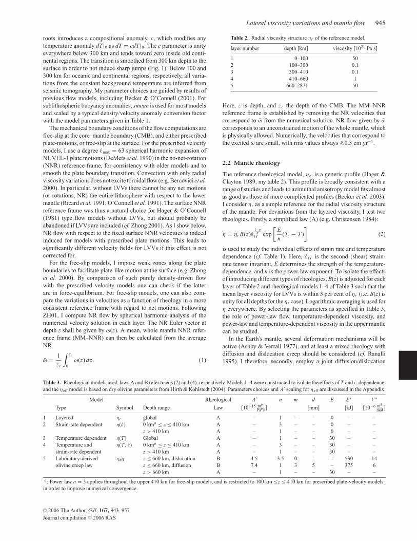
Table 3. Rheological models used, laws A and B refer to eqs (2) and (4), respectively. Models 1–4 were constructed to isolate the effects of T and ε-dependence,

and the ηeff model is based on dry olivine parameters from Hirth & Kohlstedt (2004). Parameters choices and A′ scaling for ηeff are discussed in the Appendix.

Model Rheological A′ n m d E E∗ V ∗

Type Symbol Depth range Law [10−15 mm

Pan s ] [mm] [kJ] [10−6 m3

mol ]

1 Layered ηr global A – 1 – – 0 – –

2 Strain-rate dependent η(ε) 0 kma ≤ z ≤ 410 km A – 3 – – 0 – –

z > 410 km A – 1 – – 0 – –

3 Temperature dependent η(T) Global A – 1 – – 30 – –

4 Temperature and η(T, ε) 0 kma ≤ z ≤ 410 km A – 3 – – 30 – –

strain-rate dependent z > 410 km A – 1 – – 30 – –

5 Laboratory-derived ηeff z ≤ 660 km, dislocation B 4.5 3.5 0 – – 530 14

olivine creep law z ≤ 660 km, diffusion B 7.4 1 3 5 – 375 6

z > 660 km A – 1 – – 30 – –

a: Power law n = 3 applies throughout the upper 410 km for free-slip models, and is restricted to 100 km ≤z ≤ 410 km for prescribed plate-velocity models

in order to improve numerical convergence.

Table 2. Radial viscosity structure ηr of the reference model.

layer number depth [km] viscosity [1021 Pa s]

1 0–100 50

2 100–300 0.1

3 300–410 0.1

4 410–660 1

5 660–2871 50

Here, z is depth, and zc the depth of the CMB. The MM–NNR

reference frame is established by removing the NR velocities that

correspond to ω from the numerical solution. NR flow given by ω

corresponds to an unconstrained motion of the whole mantle, which

is physically allowed. Numerically, the velocities that correspond to

the excited ω are small, with rms values always <∼0.3 cm yr−1.

2.2 Mantle rheology

The reference rheological model, ηr, is a generic profile (Hager &

Clayton 1989, my table 2). This profile is broadly consistent with a

range of studies and leads to azimuthal anisotropy model fits almost

as good as those of more complicated profiles (Becker et al. 2003).

I consider ηr as a simple reference for the radial viscosity structure

of the mantle. For deviations from the layered viscosity, I test two

rheologies. Firstly, a simplified law (A) (e.g. Christensen 1984):

η = ηr B(z)ε1−n

nI I exp

[E

n(Tc − T )

](2)

is used to study the individual effects of strain rate and temperature

dependence (cf. Table 1). Here, εI I is the second (shear) strain-

rate tensor invariant, E determines the strength of the temperature-

dependence, and n is the power-law exponent. To isolate the effects

of introducing different types of rheologies, B(z) is adjusted for each

layer of Table 2 and rheological models 1–4 of Table 3 such that the

mean layer viscosity for LVVs is within 3 per cent of ηr (i.e. B(z) is

unity for all depths for the ηr case). Logarithmic averaging is used for

η everywhere. By selecting the parameters as specified in Table 3,

the role of power-law flow, temperature-dependent viscosity, and

power-law and temperature-dependent viscosity in the upper mantle

can be studied.

In the Earth’s mantle, several deformation mechanisms will be

active (Ashby & Verrall 1977), and at least a mixed rheology with

diffusion and dislocation creep should be considered (cf. Ranalli

1995). I therefore, secondly, employ a joint diffusion/dislocation

C© 2006 The Author, GJI, 167, 943–957

Journal compilation C© 2006 RAS

946 T. W. Becker

creep law for the upper mantle which is based on the compilation

of laboratory results for olivine deformation by Hirth & Kohlstedt

(2004), as used, for example, by Billen & Hirth (2005). An effective

viscosity (law B)

εtotal = εdisl + εdiff (3)

ηeff = ηdislηdiff

ηdisl + ηdiff

(4)

is computed based on diffusion and dislocation creep viscosities

(ηdiff and ηdisl, respectively). A general, laboratory derived creep

law at constant water and melt content for these viscosities can be

written as

η =(

dm

A′

) 1n

ε1−n

nI I exp

(E∗ + pV ∗

n RTr (Tc + T )

), (5)

with parameters as given in Table 3. Here, d denotes grain size,

m grain-size exponent, E∗ and V ∗ activation energy and volume,

respectively, T r absolute reference temperature, and R the gas con-

stant. A′ is a constant that incorporates water and melt content and

a conversion of laboratory creep laws for uniaxial straining un-

der a differential stress to a regular viscosity law in SI units (see

Appendix). Viscosity laws (2) and (5) can be related. If we choose

the pre-exponential factors of both viscosities such that they yield

the same value at reference conditions p = 0, n = 1, T = T c, the

temperature-dependence is equal for T c = 1 if E = E∗/(4RT r ).

Rheology (5) needs further thermodynamic properties. To estimate

pressure, p, in the upper mantle, I use an approximate relationship

based on PREM (Dziewonski & Anderson 1981)

p(z) ≈ 105 + 3.0429 · 107z + 7.687 · 103z2,

where p is in Pa, and z in km. The pressure increase with depth

is moderated in nature by an adiabatic temperature increase. The

reference temperature T r is set to 1583◦K within the lithosphere

and increases by 0.5◦K km−1 for depths below 100 km in the upper

mantle. Within the lithosphere, a roughly error-function type of

dependence is incorporated by the tectonic T model as described

above (Fig. 1).

Seismic anisotropy is predominantly found in the boundary lay-

ers of the mantle (e.g. Montagner 1998). A common explanation

for this is that lattice preferred orientation (LPO) anisotropy of

olivine forms under dislocation creep, and that this mechanism

should be dominant at relatively shallow (high-stress, low tempera-

ture) depths (e.g. Karato 1998; Hirth & Kohlstedt 2004). However,

seismic anisotropy studies can, at present, not put firm constraints

on the depth extent of dislocation creep (e.g. Trampert & van Heijst

2002; Wookey & Kendall 2004). I shall nonetheless proceed to fo-

cus on the role of power-law behaviour for the uppermost mantle for

simplicity. Power-law creep is thus restricted to the upper 410 km

for law A (see Table 3), or to the upper mantle as governed by the

joint rheology (law B). Law B is certainly closer than law A to what

we would expect from laboratory measurements for upper mantle

olivine rheology. However, it is not clear which parameters (e.g. d,

V ∗, water content) apply for nature. Often the creep law parameters

are, therefore, treated as adjustable to tune the transition between

dislocation and diffusion dominated flow (e.g. McNamara & Zhong

2004). I have done the same here and will mostly discuss results for

law B using dry olivine parameters as detailed in the Appendix.

In the case of the free-slip models, I additionally reduce the reg-

ular viscosity in the upper 100 km within 100 km distance from

NUVEL-1 plate boundaries by a factor of 100 to allow for plate-

like motion (Zhong et al. 2000). Particularly for the T-dependent

viscosity models, this is needed to not be in an entirely stagnant-lid

regime at low temperatures. Details of the weak-zone formulation

will be important for the magnitudes of plate velocities (King &

Hager 1990; King et al. 1992; Yoshida et al. 2001), but I am not

concerned with exact model predictions here. For all rheologies, η

is restricted to only vary from 1017 to 1024 Pa s for numerical sta-

bility. In the case of the upper-end truncation, this procedure may

be considered as a rough approximation of plastic yielding at low

temperatures close to the surface (Goetze & Evans 1979). I have

conducted a few tests for different viscosity cut-off ranges, main

conclusions presented here are not dependent on this choice.

2.3 Numerical approach

The Stokes equations in the Boussinesq approximation are solved

for instantaneous circulation with the spherical finite element (FE)

code CitcomS (Zhong et al. 2000) from geoframework.org; the

original, Cartesian version was developed by Moresi & Solomatov

(1995). CitcomS is well benchmarked and the implemented multi-

grid solver is capable of treating LVVs at high resolution. For most

computations, I use 196 608 elements laterally (∼25 km element

width at the surface), and 129 elements radially. The vertical spacing

of elements is∼10 km in the upper mantle above 660 km and∼35 km

below. All model velocities were interpolated on 1◦ × 1◦ grids in 44

layers for further visualization and analysis. With a lower resolution

at a quarter of the number of elements, I was able to reproduce ηr

Hager & O’Connell (1981) solutions with <∼2 per cent rms velocity

differences. Increasing the resolution to the full number of elements

which is used here led to changes in velocities of a few percent for

power-law computations, and I expect further refinement to lead to

insignificant modifications.

For power-law viscosities, I iterate the FE velocity solution until

the rms of the incremental change in velocities is below 1 per cent

of the rms of the total velocity field. It was beneficial in some cases

to perform this iteration in a damped fashion, using only a fraction

(∼0.75) of the new solution with updated viscosities for the next

iteration step. For prescribed plate velocities with large strain rates

across plate boundaries, it was not possible to reduce this mean dif-

ference between incremental velocity solutions during power-law

loops to below ∼3 per cent. I, therefore, only report results for pre-

scribed velocity models where the lithosphere (z < 100 km) remains

Newtonian. However, the velocities for full power-law computations

are very similar to those shown here. The NR component for pre-

scribed velocity models is somewhat sensitive to the choices as to

the power-law iteration, and was observed to typically increase by

∼15 per cent between 3 and 1 per cent rms velocity changes.

3 R E S U LT S A N D D I S C U S S I O N

First, example maps of velocities for different rheological models

are presented. I then show both models with prescribed surface ve-

locities and for free-slip; results are similar, indicating that model

assumptions are dynamically consistent. Second, a quantitative anal-

ysis of similarities and differences between the rheological and flow

character of the models is performed. This leads to a discussion of

toroidal flow, and of net rotations of the lithosphere in particular. I

conclude by commenting on implications for fitting observed plate

motions.

C© 2006 The Author, GJI, 167, 943–957

Journal compilation C© 2006 RAS

Lateral viscosity variations and mantle flow 947

Figure 2. Flow velocities (fixed length vectors, amplitudes given by right colour bar and layer rms by lower right label, respectively, units of cm yr−1) and

viscosity variation from the layer mean (log10(η) − 〈log10(η)〉, where 〈〉 indicates the average, as specified on lower left of figures, units of 1021 Pa s) at a depth

of 250 km for plate-motion prescribed models. Velocities are given in the mean mantle NNR reference frame. Plots (a), (b), (c), and (d) show results for the

radial reference model, ηr , pure power law, η(ε), T -dependent viscosity, η(T), and for power law plus T-dependence, η(T, ε), model, respectively (see Table 3).

Compare with Fig. 3 for free-slip models.

3.1 Velocity maps

Fig. 2 shows velocities and LVVs with respect to the layer mean

for the velocity-prescribed models for the four rheological set-ups

1–4 of Table 3. I show flow in the MM–NNR reference frame at a

depth of 250 km. Comparison of reference model a) with the pure

power-law computation (Fig. 2b) shows that strain-rate dependent

creep alone does not modify the circulation pattern substantially,

though it does lead to larger velocity amplitudes in regions such as

the NW Pacific. Following the distribution of induced strain rates,

the viscosity is decreased underneath some oceanic plates, and par-

ticularly underneath a few continental regions such as western North

America and central Europe. Such LVVs and corresponding differ-

ences in velocities are found at the boundaries of the composition-

ally distinct regions (cf. Fig. 1). The relatively stagnant keels lead

to regions of weakened viscosity around them. This effect is ab-

sent in models that have no lateral compositional differences; pure

power-law flow for these models is then very similar to the refer-

ence model, with slight weakening of average viscosity underneath

oceanic plates. The finding that pure power-law flow is similar to

Newtonian flow is consistent with early findings for 2-D thermal

convection (Parmentier 1978; Christensen 1984), and with Cadek

et al.’s (1993) study. It is also not too surprising given the fairly

smooth lateral density variations as inferred from global tomogra-

phy or my tectonic model. Comparison of Figs 2(a) and (c) shows

that temperature-dependent viscosity does lead to some rearrange-

ment in flow patterns, most pronounced underneath oceanic plates

where tomographic anomalies are mapped into LVVs. Correspond-

ingly, velocity directions are different, for example, for η(T) in the

super-swell region in the southwest Pacific, and within a channel

that roughly parallels the East Pacific Rise (EPR) at a distance of

∼1250 km to the west. Flow patterns close to this anomalous chan-

nel have been discussed by Gaboret et al. (2003) in the context of

seismic anisotropy for a ηr -type flow model. Further analysis (not

shown) reveals other regions where flow is affected by temperature-

dependent viscosity: underneath the ridges themselves and in areas

with fast, presumably subduction-related, tomographic anomalies

(‘slabs’), such as under central North America. Such modifications

in flow are caused both by the stirring action of strong continental

roots (Zhong 2001; Cadek & Fleitout 2003) and by the relatively

weak material underneath oceanic plates.

The η(T) model also differs from ηr flow in terms of the velocity

amplitudes. At 250 km depth η(T) shows larger velocities on av-

erage, with global rms (maximum) values increased from 2.9 (6.8)

(Fig. 2a) to 4.2 (33.2) cm yr−1 (Fig. 2c). Velocities for LVV flow are

enhanced by up to a factor of ∼30 underneath the channel anomaly,

and by factors of ∼10 underneath some of the ridges. Adding power-

law creep to the temperature-dependent viscosity (Fig. 2d) reduces

the LVVs. This is expected from the reduced effective temperature-

dependence, E/n in eq. (2), and the regulating effects as seen in

thermal convection models (Christensen 1984). Accordingly, rms

and maximum velocities at 250 km depth are reduced to 3.9 and

25.1 cm yr−1, respectively, for η(T, ε). The geographic distribu-

tion of deviations in terms of velocity patterns is different between

the η(T, ε) and η(T) model. Adding strain-rate weakening tends to

emphasize the velocity discrepancies in regions of upwellings such

as the East African Rift and the channel anomaly. However, flow

around slabs appears more similar to ηr for η(T, ε) than for η(T),

as the relative strength contrast of the cold anomalies is lower for

models that incorporate strain-rate dependent viscosities.

Surface wave tomography clearly images half-space cooling

structure underneath oceanic plates up to depths of ∼150 km

(e.g. Ritzwoller et al. 2004). This is expected from the com-

mon geodynamic point of view where mostly passive spreading

at the ridges transitions to cooling of oceanic plates toward the

trenches. Somewhat unexpected is that slow vS is commonly found

C© 2006 The Author, GJI, 167, 943–957

Journal compilation C© 2006 RAS

948 T. W. Becker

Figure 3. Velocities and viscosity variation at 250 km for free-slip convection models with different rheological set-ups, for description see Fig. 2.

underneath major ridges up to depths of ∼300 km (e.g. Becker &

Boschi 2002). Correspondingly, my models exhibit a broad, low

viscosity ‘asthenosphere’ underneath the ridges, as η(T) depends

on the scaled d ln vS-anomalies. To test the importance of subo-

ceanic anomalies within the upper 300 km, I also computed flow

for η(T, ε) models where no tomographic structure was used for

the upper 300 km anywhere. Only half-space cooling and stiff con-

tinental roots were imposed, which in itself leads to relatively low

viscosity underneath the oceanic plates (Cadek & Fleitout 2003).

The large-scale flow patterns of such a simplified LVV model are

similar to what is shown in Fig. 2(d). The stirring action of the

prescribed continental roots is, however, more pronounced, as there

are few other anomalies in the shallowest mantle. Consequently,

large differences between ηr and η(T, ε) flow are found close to

the roots. The channel anomaly east of the EPR persists, indicating

that buoyancy sources deeper than ∼300 km are important for this

pattern. Average velocity amplitudes at 250 km are reduced to 3.5

from 3.9 cm yr−1 in Fig. 2(c), and the maximum velocities are only

10.4 cm yr−1 without the shallow anomalies.

Are the velocity results and rheology consistent with regard to

driving forces, or are they artefacts induced by the prescribed plate

motions? Fig. 3 shows velocities at 250 km for the same rheolog-

ical and density set-ups but free-slip/weak-zone surface boundary

conditions. The general flow patterns of Fig. 3 match those of Fig. 2

well. This is not surprising, as we know that global circulation mod-

els are able to predict plate motions (e.g. Ricard & Vigny 1989;

Lithgow-Bertelloni & Richards 1998; Zhong 2001). However, the

match is reassuring, and also the general behaviour of flow mod-

ification as a function of rheology is similar for the free-slip and

prescribed plate-motion models. The rms and maximum velocities

at 250 km depth are 2.9 (6.8), 3.9 (34.6) and 4.4 (19.8) cm yr−1 for

the reference, η(T), and η(T, ε) model, respectively. Below, the fit

to present-day plate motions is discussed further.

In terms of rheology, there are no significant global differences

we can distinguish visually between Figs 2 and 3. This implies that

the prescribed surface velocities of Fig. 2 do not unduly constrain

the large-scale variations in strain rate compared to freely deform-

ing models. The geographic regions where η(T ) and η(T, ε) models

show strongly different velocities from ηr flow are more confined

for the free-slip models than for the prescribed velocity approach.

In terms of orientations, the deviations are more focused under-

neath ridges and much reduced underneath central North America

as well as around slab regions. While the channel anomaly is still

a strong feature for different rheological models for free-slip, it is

more focused toward the SW of the EPR. These regional differ-

ences between Figs 2 and 3 imply that in those locations, the purely

buoyancy-driven flow does not closely match the velocities of the

prescribed velocity approach. The situation in nature will likely fall

somewhere in between my simplified end-member cases.

3.2 Average viscosity profiles

Fig. 4 shows the depth dependence of the logarithmic mean of the

of viscosity and its rms variation for models with η(T ), η(T, ε)

and ηeff rheologies (Table 3). These averages were calculated for

free-slip circulation as shown in Figs 3(c) and (d). However, the

corresponding results for the prescribed velocity computations are

very similar. My particular choice of temperature-dependence (E =30 for model η(T)) leads to viscosity variations up to ∼1.5 orders

of magnitude in terms of rms variations (Fig. 4a). The maximum

variability is found in the upper boundary layer at ∼150 km, as

expected from the variation of tomographic anomaly strength with

depth (e.g. Becker & Boschi 2002) and thermal convection computa-

tions (e.g. Zhong et al. 2000). When the mean viscosity is computed

underneath oceanic and continental regions separately, a ∼ one order

of magnitude difference is predicted for purely T-dependent viscos-

ity between 100 km and 410 km depth. Even though the average

for the 0–100 km layer for η(T) is made to match the ηr value of

5 · 1022 Pa s, the mean surface viscosity is ∼5 · 1023 Pa s which

implies relatively sluggish surface motions.

So far, no flow computation would have been necessary for these

statements about η(T) viscosities. However, the evaluation of con-

sistent strain rates becomes important for power-law computations

C© 2006 The Author, GJI, 167, 943–957

Journal compilation C© 2006 RAS

Lateral viscosity variations and mantle flow 949

(a) η T 0

500

1000

1500

2000

2500

-3 -2 -1 0 1 2 3

depth

[km

]

log10(η/1021

Pas)

meanocean

contrms

(b) η T ε

-3 -2 -1 0 1 2 3

log10(η/1021

Pas)

meanocean

contrms

(c) ηeff

-3 -2 -1 0 1 2 3

log10(η/1021

Pas)

meanocean

contrms

-1 0 1

log10(εdisl/εdiff)

Figure 4. Depth dependence of log -averaged viscosity and rms deviations for rheological models η(T) (a), η(T, ε) (b), and ηeff (c) for the free-slip models

of Fig. 3. Black solid lines indicate the mean (constrained to match ηr to within 3 per cent for models a and b), and grey-solid and dashed-black lines denote

the mean underneath oceanic and continental regions (from 3SMAC), respectively. The dashed-grey line indicates the rms variations of log10(η). For the joint

diffusion/dislocation creep rheology of the ηeff model (c), I also show the mean ± rms of the strain-rate partitioning (see eqs 4 and 6).

(Figs 4b and c). The regional discrepancy of viscosity averages

underneath oceanic and continental plates, and the total η variabil-

ity, are reduced by the introduction of power-law flow, as mentioned

for the 250 km depth layer example above. A factor∼5 difference be-

tween average η underneath oceanic and continental plates is found

for η(T, ε), suboceanic viscosities are weaker by ∼3 if we remove

the anomalies inferred from tomography above 300 km. Surface

viscosities for η(T, ε) are smaller than for η(T), as the power-law

dependence weakens the thermally-induced high viscosity lid.

The reduction of variability in η due to introduction of strain-

rate weakening becomes important if we wish to evaluate mantle

tractions for plate coupling models (Cadek & Fleitout 2003), as

those tractions scale with the viscosity contrasts (Conrad & Lithgow-

Bertelloni 2006). Given the results shown in Figs 2–4, it appears

feasible to derive an effective T-dependent rheology with reduced

temperature dependence E ′ ∼ E/n, whose tractions and viscosity

variations match those of a more complete, η(T, ε), rheology. Such

a rescaling was detailed by Christensen (1984) for 2-D convection,

but the establishment of a quantitative relationship is outside the

scope of this paper.

Models η(T) and η(T, ε) were constructed to isolate the effects

of ε and T on viscosity, and were constrained to match the radial

average ηr . As a check, Fig. 4(c) shows results for the joint dislo-

cation/diffusion creep rheology, ηeff, that is based on olivine creep

laws. For the choice of laboratory-derived parameters in Table 3, it is

possible to obtain a depth-averaged viscosity structure that roughly

resembles ηr , both for the prescribed surface velocity and the free-

slip models. The offset of the suboceanic and continental viscosity

averages is confirmed for this model. While mostly a direct con-

sequence of my input model choices (e.g. strong continental roots

up to 300 km), it is interesting that all models are consistently pro-

ducing an oceanic asthenosphere that is ∼ one order of magnitude

weaker than the subcontinental regions in the transition zone (cf.Cadek & Fleitout 2003).

Taking the compilation of Hirth & Kohlstedt (2004) at face value

for rock behaviour in the upper mantle, I found that wet parameters

led to average viscosities that were about a factor of ∼50 lower than

those of ηr between ∼150 and 500 km. Minimum 〈η〉 viscosities at

∼200 km depth are 4.4 · 1018 and 1.4 · 1018 Pa s for water contents

of C OH = 100 and 1000 H/106Si, respectively (see Appendix), com-

pared to 8.9 · 1019 Pa s for ηeff as shown. The better match between

average viscosities is why I used dry values for A′ and creep law pa-

rameters. For the ηeff model with free-slip boundary condition and

weak zones as shown in Fig. 4(c), log -averaged εI I values for the

four upper mantle layers of Table 2 are ≈2, 42, 19, and 8 · 10−16 s−1,

and 2 · 10−16 s−1 for the lower mantle. For the prescribed surface

velocity ηeff model, all εI I averages are similar to the free-slip case,

but the top 100 km average is only 1 · 10−16 s−1.

I measure the partitioning between dislocation and diffusion creep

by

γ = log10(εdisl/εdiff), (6)

meaning that γ 0 corresponds to dislocation-creep dominated

deformation, and vice versa. The average 〈γ 〉 and its rms variations

in the upper mantle are shown in the subplot of Fig. 4(c) for the

ηeff model. For the modelling choices of Table 3, γ crosses zero at

∼300 km depth. This transition depth and the general shape of 〈γ 〉for the joint rheology are broadly consistent with LPO dominated

seismic anisotropy in the uppermost mantle forming under dislo-

cation creep (cf. Podolefsky et al. 2004). At depths which are pre-

dominantly in the dislocation creep regime, for example, at 200 km,

the cold, stiff continental roots as well as regions around slabs show

the largest γ , consistent with results by McNamara et al. (2003).

At the same depths, some oceanic regions close to ridges are pre-

dicted to be in the diffusion creep regime with γ < 0. Details in

the dependence of 〈γ 〉 on depth such as the zero-crossing (i.e. the

average transition stress between dislocation and diffusion creep)

depend strongly on the creep law parameters such as d. However,

the overall shape of 〈γ 〉 and regional patterns in γ are more robust

with regard to parameter choices. The spatial distribution of γ are

of interest for the study of LPO development.

The results with regard to the effective viscosity creep-law are

dependent on the rheological parameters, which are not particularly

well constrained, even for the upper mantle. However, the main

point here is that it is possible to construct a dynamically plausi-

ble flow model, like my ηeff case. This set-up is broadly consistent

with canonical radial viscosity averages such as ηr, with laboratory

findings on rheology, and with the present understanding of LPO

anisotropy.

C© 2006 The Author, GJI, 167, 943–957

Journal compilation C© 2006 RAS

950 T. W. Becker

(a) plate motions prescribed

0

500

1000

1500

2000

2500

0.6 0.7 0.8 0.9 1

depth

[km

]

ξ

η(ε)η(T)

η(T),NR

η(T,ε)ηeff

-0.2 0 0.2

α 0 0.5 1 1.5

ν

(b) free-slip with weak zones

0

500

1000

1500

2000

2500

0.6 0.7 0.8 0.9 1

depth

[km

]

ξ

η(ε)η(T)

η(T,ε)ηeff

-0.2 0 0.2

α 0 0.5 1 1.5

ν

Figure 5. Depth dependence of the mean, velocity-weighted dot product of normalized velocities (ξ = 〈vn .vnr 〉|v||vr |, left), mean of the logarithmic velocity

amplitude ratio (α = 〈log10(|v|/|vr |)〉, centre), and NR amplitude as a fraction of GJ86 of each velocity layer (ν, right subplots) for different rheological models

v (see Table 3). All comparisons use the ηr model as the reference (vr ). Figure (a) compares velocities for models where plate velocities were prescribed at

the surface in a NNR reference frame. However, any layer NR was removed before computing ξ or α for all cases but ‘η(T) NR’, which compares the full η(T)

and ηr velocities. Plot (b) compares free-slip, weak zone models in a consistent, mean mantle MM–NNR reference frame.

3.3 Quantitative comparison of velocity fields

Fig. 5 shows global velocity variations as a function of rheology and

depth. I compute a correlation-like measure

ξ = ⟨vn .vn

r

⟩|v||vr | (7)

from a weighted average of the dot product of the normalized

test (LVV) and reference (ηr ) model velocities, vn = v/|v| and

vnr = vr/|vr |, respectively. where |.| denotes the vector norm. The

global mean is weighted by the product of the local velocity am-

plitudes of the fields to give more weight to regions that exhibit

stronger flow. (ξ is typically larger by ≈0.05 than an unweighted

mean correlation 〈vn . vnr 〉.) For analysis of amplitude changes, a

mean logarithmic amplitude ratio referenced to ηr , is used

α = 〈log10(|v|/|vr |)〉. (8)

Fig. 5 also shows the NR component of the velocities at each depth,

normalized by the amplitude of NR in the GJ86 hotspot reference

Table 4. NR Euler vectors, ω (0), of the lithosphere as inferred from hotspot

reference models and numerical computations (free-slip in the mean-mantle

NNR reference frame). Model labels refer to those used in Fig. 6.

Model Reference Longitude Latitude Amplitude

label [◦ Myr−1]

Plate reconstruction models

GJ86 Gordon & Jurdy (1986) 37◦E 40◦S 0.115

T22 Wang & Wang (2001) 88◦E 62◦S 0.142

HS3 Gripp & Gordon (2002) 70◦E 56◦S 0.436

SB04a Steinberger et al. (2004) 38◦E 40◦S 0.165

Geodynamic free-slip computations

Z01 case 4 of Zhong (2001) 103◦E 42◦S 0.092

η(ε) 33◦E 33◦N 0.023

η(T) 97◦E 54◦S 0.087

η(T, ε) 71◦E 46◦S 0.114

ηeff 94◦E 45◦S 0.088

Note: aThe SB04 pole is an updated hotspot reference frame estimate using

the procedure of Steinberger et al. (2004) (B. Steinberger, personal

communication, 2006).

model by Gordon & Jurdy (1986) (see Table 4):

ν = |ω||ωG J86(0)| . (9)

Fig. 5(a) shows how velocity solutions vary from those of the

reference model, ηr, for model rheologies 2–5. A substantial NR

component of flow is introduced by all models with LVVs. This

is particularly evident for models with T-dependent viscosity. For

such cases, the NR reaches ∼1–1.5 the GJ86 hotspot reference-

frame values at ∼400 km depth, even though the surface velocities

were constrained to be in the NNR reference frame. This implies that

NNR plate motions are physically incompatible with the rheological

models. If these NR components of flow are not accounted for,

velocity predictions for LVV models can be quite different from

those for ηr models at depths larger than ∼400 km. This can be seen

by the comparing ξ for velocities from the original η(T) solution

(thin grey line) with ξ for velocities which had any NR component

at each layer removed (all other graphs in the left portion of Fig. 5a).

I return to the question of reference frames below. Here, all other ξ

and α measures for the plate-driven models in Fig. 5(a) are computed

after a layer-based NR correction is applied: At each depth level,

the NR is computed and subtracted from the velocities. Conversely,

Fig. 5(b) uses a consistent MM–NNR reference frame.

Comparing ξ for the different rheological models in Fig. 5(a), I

find that pure power-law flow models are indeed very similar at ξ >∼0.92 at all depths, as expected. Introducing T-dependent η reduces

the correlation to minimum values of ξ ∼ 0.75. Such deviations in

velocity fields are comparable to other uncertainties, such as those

due to our incomplete knowledge about the temperature structure

of the mantle. As anticipated above, the joint η(T, ε) model leads

to smaller deviations from ηr (black dashed line in Fig. 5a). For the

particular choices of Table 3, the effective viscosity model leads to

variations in velocities that are similar to the η(T) case. Mean vari-

ations in amplitude of flow are quite small (mid plot of Fig. 5a) but

for the ηeff model at ∼400 km. The ηeff case is the only one where

average layer viscosities were not formally constrained to match ηr ,

so this comparison is somewhat misleading. Most changes in am-

plitude α for η(T ) and η(T, ε) are due to faster flow underneath the

oceanic plates (cf. Fig. 2). The ξ and α values in Fig. 5(a) imply

C© 2006 The Author, GJI, 167, 943–957

Journal compilation C© 2006 RAS

Lateral viscosity variations and mantle flow 951

that the gross structure of flow will be similar for different rheo-

logical model predictions. However, regionally, deviations such as

in the SW Pacific (cf. Figs 2 and 3) may be important. Using re-

gional predictions and constraints such as from seismic anisotropy

may in fact allow to put further bounds on the rheology of the

mantle.

The details of the depth dependence of the quantities computed

for Fig. 5 depend on ηr , and in particular the low viscosity channel

from 100 to 410 km (Table 2). However, I also computed velocities

for a simpler ηr viscosity with only three layers (ηr (100 km ≤ z ≤660 km) = 1021 Pa s). Results are broadly consistent with, but ex-

pectedly smoother than, those presented in Fig. 5. The amplitudes

and the trend among different rheological models for ξ is preserved

for the simpler ηr. Amplitude ratio variations are closer to zero than

for the ηr used for Fig. 5, with slight α < 0 velocity reduction in

the upper mantle for laterally varying viscosity models. I also tested

ngrand (Grand 2001) as an alternative seismic tomography model

to infer temperature. Results are again similar to what is shown in

Fig. 5(a), with larger rms viscosity variations for η(T) models than

for smean. Such behaviour is expected given that ngrand has more

power at higher spatial frequencies than smean (Becker & Boschi

2002). While trends between different rheological models are pre-

served, minimum ξ values are reduced by ∼0.1 compared to Fig. 5(a)

for ngrand.

Fig. 5(b) repeats the comparison among rheological models for

the respective free-slip computations. Velocities were transformed

into the MM–NNR reference frame. The general findings as to the

different degrees of similarity for rheological models as expressed

by ξ are confirmed for these self-consistent models. Congruent with

Conrad & Lithgow-Bertelloni (2006) study, my results indicate that

the variations in the directions of flow, and hence tractions, are

moderate when more realistic rheologies are incorporated in mantle

flow models. Correlation values are always ξ >∼ 0.8 in the upper-

most mantle (z >∼ 200 km), and do not drop below ξ ∼ 0.7 when

they are least similar at ∼400 km depth. Amplitude variations with

depth among different free-slip models are moderate for all but the

η(T) and ηeff models in Fig. 5(b). The relatively slow velocities for

these strongly temperature-dependent cases are caused by the large

surface viscosities mentioned above. Introducing strain-rate weak-

ening rheologies allows the plates to move more freely for η(T, ε)

(cf. Solomatov & Moresi 1997; Zhong et al. 1998), but also leads

to a loss of plateness in my large-scale flow models, as discussed

below.

3.4 Generation of net lithospheric motion by stiff

continental roots

3.4.1 Net surface rotation

For free-slip models, the choice of velocity reference frame is ar-

bitrary (Zhong 2001). However, the mean mantle NNR reference

frame is appealing, and makes it easier to study the generation of

net motion. The right subplot of Fig. 5(b) shows that all models

with LVVs excite a NR component of flow which is focused in the

upper ∼400 km. A very similar depth dependence was documented

by ZH01. The NR component of the ηr free-slip model should be

exactly zero from theory, and is always ν < 0.1 per cent when com-

puted numerically. This number provides a bound on the accuracy of

the FE method and the velocity analysis procedure. For my free-slip

models with LVVs in the MM–NNR frame, the lithosphere moves

with regard to a relatively stable lower mantle with a sense that is con-

sistent with hotspot reference frames such as HS3 (Table 4). Zhang

& Christensen (1993), Cadek et al. (1993) and Wen & Anderson

(1997) previously studied the excitation of NR in global, spherical

models. These studies, however, found that neither amplitudes, nor

directions of NR motion were matched well compared to a hotspot

reference. One reason for this may be that very little toroidal motion,

such as NR flow, is excited for purely temperature-dependent LVVs

(Christensen & Harder 1991; Ogawa et al. 1991). Bercovici et al.(2000) suggest that in order to efficiently generate toroidal flow, it is

necessary that buoyancy and viscosity anomalies are spatially out of

phase. Such conditions are given for the case of weak zones at plate

boundaries (e.g. Zhong et al. 1998) or non-linear, strain-weakening

rheologies (Bercovici 1995; Tackley 2001b).

More recently, Zhong (2001) showed that strong continental roots

and weak zones can indeed generate NR motion of the lithosphere,

and my findings are consistent with his results. ZH01 varied the

depth of the roots to analyse their effect on the generation mecha-

nism and found that the deepest continental roots that were consid-

ered (down to 410 km depth) were able to generate the largest NR

motion, ν ≈ 80 per cent. Table 4 provides an overview of published

estimates of net lithospheric rotation in hotspot reference frames;

Euler pole locations are plotted in Fig. 6. The exact nature of the ob-

served net motion of the present-day plates with regard to hotspots is

debated and intimately related to the question of hotspot-fixity with

respect to the lower mantle. If motions of hotspots are accounted for

(Steinberger et al. 2004), amplitudes of NR are reduced compared

to the HS3 model, but still larger than GJ86 (Table 4). I, therefore,

compare previous and my modelling results for net rotations with a

range of published models (Fig. 6).

Using the general geodynamic model set-up, I find that strain-rate

dependence with n = 3 and weak zones alone are ineffective in intro-

ducing NR motion (cf. Cadek et al. 1993; Bercovici 1995); rotation

poles are far from published hotspot estimates (Fig. 6). However,

when temperature-dependent viscosities are introduced on top of the

weak-zone formulation, the pole moves closer to estimates such as

HS3

SB04

GJ86

T22

Z01

η(ε)

η(T)

η(T,ε)ηeff

Figure 6. Location and magnitude (circle radius) of NR Euler poles from

several hotspot reference models and my geodynamic computations, labels

and values given in Table 4.

C© 2006 The Author, GJI, 167, 943–957

Journal compilation C© 2006 RAS

952 T. W. Becker

HS3 (Fig. 6). Amplitudes reach 76 per cent of the GJ86 estimates,

or 20 per cent of HS3 for η(T). This finding substantiates results

by ZH01, at somewhat reduced continental root depths compared to

that study. Interestingly, the power-law rheology of η(T, ε) enhances

the NR component, up to 99 per cent of GJ86 or 26 per cent of HS3.

The predicted Euler pole locations of my free-slip models are given

in Table 4 and Fig. 6 and match those of HS3 closely. It seems that

the rheologies employed in this study lead to somewhat larger NR

amplitudes than those used in ZH01.

3.4.2 Toroidal:poloidal partitioning

The enhanced generation of net motions is related to the more ef-

fective generation of toroidal flow by η(T, ε) models. One common

diagnostic measure is the ratio between toroidal and poloidal veloc-

ity fields at the surface (O’Connell et al. 1991; Tackley 2001a). I

compute the toroidal:poloidal ratio i as

i = pti

p pi

, (10)

where p p,ti is the total power of a spherical harmonic expansion of

the velocity field components,

p p,ti = 1

2√

π

√�

�max�=i ��

m=0

(a2

�m |p,t + b2�m |p,t

). (11)

Here, {a�m , b�m}| p,t are the real spherical harmonic coefficients of

the poloidal (subscript p) or toroidal (subscript t) field (as defined

in eqs. B.99 and B.158–160 of Dahlen & Tromp 1998), and I use

�max = 63.

With definition eq. (10), 1 includes the � = 1 NR component ν,

and 2 measures the toroidal:poloidal power partitioning without

NR. Table 5 lists surface and ν values for tectonic and geodynamic

models; 1 ∼ 1 for HS2 and HS3. The non-NR toroidal:poloidal

partitioning is 2 ∼ 0.5 for plate models such as NUVEL-1, and

has been at similar levels in the convective past (Lithgow-Bertelloni

et al. 1993). Since the surface ratio of toroidal to poloidal power

has a white spectrum (O’Connell et al. 1991), details such as the

Table 5. Surface velocity diagnostics for tectonic and geodynamic free-slip models: �: plateness (eq. 13), �: oceanic to continental rms speed

ratio, ξ (0): similarity of predicted surface velocities to NUVEL-1 plate motions (eq. 7), 1(0), 2(0): toroidal: poloidal power ratio with and

without the NR component (eq. 10), and ν(0): NR normalized by GJ86 (eq. 9, see Table 4). (Parameters ξ , i and ν are evaluated at the surface.)

Velocities from the free-slip, weak-zone models are computed in the MM–NNR frame, may include an NR component for the LVV cases, and

should thus be compared with hotspot reference frame tectonic models. All models were sampled on 1◦ × 1◦ grids. References: NUVEL-1

NNR: DeMets et al. (1990); NUVEL-1 HS2 Gripp & Gordon (1990); NUVEL-1A HS3: Gripp & Gordon (2002); GSRM-NNR: Kreemer et al.(2003).

Plateness oc/co Plate Toroidal:poloidal Net

speed motion power ratio rotation

ratio fit with ν w/o ν

Model � � ξ (0) 1(0) 2(0) ν(0)

Tectonic models

NUVEL-1 HS2 1 2.9 – 0.92 0.53 2.88

NUVEL-1A HS3 1 2.7 – 1.17 0.53 3.79

NUVEL-1 NNR 1 2.3 – 0.53 0.53 0

NUVEL-1 NNR, smoothed at �max = 63 0.87 2.3 – 0.52 0.52 0

GSRM-NNRa 0.87 2.1 – 0.57 0.57 0

Geodynamic free-slip models

ηr 0.56 1.7 0.83 0.37 0.37 0

η(ε) 0.55 1.7 0.83 0.37 0.37 0.20

η(T) 0.96 3.0 0.93 0.55 0.43 0.76

η(T, ε) 0.51 2.5 0.90 0.42 0.38 0.99

ηeff 0.91 3.2 0.95 0.58 0.50 0.76

Note: aSince the GSRM-NNR model is not global, the polar regions were interpolated based on best-fit rigid plate motions for the Antarctic,

North American and Eurasian plate.

tapering of my spherical harmonic expansion of NUVEL-1 do not

affect 2 much (Dumoulin et al. 1998).

Table 5 compares surface velocity diagnostics for tectonic mod-

els and those computed from free-slip convection computations. The

toroidal:poloidal ratio for ηr is 1,2 = 0.37 which indicates the effect

of the weak zones. The imposed plate geometry in itself generates

toroidal motion and organizes the flow (Gable et al. 1991), in partic-

ular for motions on the surface of a sphere (O’Connell et al. 1991;

Olson & Bercovici 1991). Introducing power-law rheology alone

does not increase the toroidal power, as expected from Bercovici

(1995) experiments. However, all LVV models with temperature-

dependent viscosity have increased 2 of 0.4–0.5. Those values are

comparable to the toroidal power in NUVEL-1 (for � ≥ 2, Table 5).

The ηeff case shows 2 toroidal power that is similar to NUVEL-

1 values and larger than 2 for η(T, ε). Since the NR of ηeff is

smaller than that of η(T, ε), this means that surface velocities of

ηeff are more Earth-like with regard to partitioning, but absolute

amplitudes of NR are slower than in hotspot reference frames. I ex-

pect NR Euler pole locations and toroidal:poloidal partitioning to

be better measures of realism than exact values of NR, ν.

3.4.3 Generation of toroidal motion

Wen & Anderson (1997) showed that the introduction of rheological

oceanic/continent differences excites toroidal flow by mode cou-

pling in their low order spherical harmonics models. My models

refine the results by Wen & Anderson, using what I consider a more

consistent approach for arriving at differences in viscosity under-

neath different plate regions. My finding of increased with LVVs

is also in agreement with ZH01, where values of 1 ∼ 0.5 were pro-

duced for the deepest continental root model, in analogy with the

discussion of the excitation of net motion above. Tackley (2001b)

studied how 2 varies with depth and found enhanced generation of

toroidal flow for some of his non-linear rheology cases. I have also

analysed 2 as a function of depth for the free-slip computations.

All models with T-dependent LVVs show larger 2(z) throughout

C© 2006 The Author, GJI, 167, 943–957

Journal compilation C© 2006 RAS

Lateral viscosity variations and mantle flow 953

the mantle than ηr or η(ε) cases. I find that the toroidal:poloidal

partitioning decreases from the surface values of Table 5 for η(T) to

a minimum at ∼2000 km depth. At greater depths, there is a slight

increase toward the CMB. This behaviour indicates a scaling of 2

with the strength of the LVVs as inferred from the d ln vS anomalies

of tomography (see also rms variations of η in Fig. 4). However,

2 increases from 2(0) ∼ 0.4 to a sublithospheric maximum of

2 ∼ 0.8 at ∼150 km for η(ε) and ηeff flow, before decreasing toward

the lower mantle (cf. Tackley 2001b). This finding substantiates that

non-linear rheologies play a role for toroidal flow generation, even

in the presence of prescribed weak zones.

Given findings by Christensen & Harder (1991), Martinec et al.(1993) and Bercovici et al.’s (2000) suggestion that pure T-

dependent convection will not be efficient in generating toroidal

flow, I also computed 2(z) for models similar to the η(T) case but

without compositional anomalies c in the continental keels. Results

were very similar to η(T) flow with compositional anomalies. If

weak zones along plate boundaries are also omitted, 2(0) drops to

zero as there is almost no motion at the surface in this rigid lid case.

However, 2 does increase to ≈ 0.45 at ∼250 km depth, and then

follows the 2(z) behaviour at depth as seen for η(T) flow with weak

zones. This finding indicates that purely temperature-dependent

LVVs can generate significant toroidal motion in global circulation

models where ‘temperature’ really means ‘scaled velocity anoma-

lies’. I conjecture that thermal convection does not generate signif-

icant toroidal flow for purely temperature-dependent viscosity, but

η(T) type flow models do as they use information from tomography,

which maps the thermo-chemical convective state of the Earth.

To evaluate the role of continental root rheology for the exci-

tation of NR further, I conducted a series of tests with strain-rate

and temperature-dependent rheology of type η(T, ε). The simplified

tectonic model without any tomographic anomalies above 300 km

is used in order to isolate the role of strong roots, whose strength

is varied by increasing the non-dimensionalized activation energy.

Fig. 7 shows how the ratio of mean cratonic or subcontinental to

ambient viscosity between 100 and 250 km depth increases with

the non-dimensional temperature-dependence E/n (n = 3, eq. 2). I

show results for both prescribed plate motion and free-slip models

(cf. ν-plots in Fig. 5). For both mechanical boundary conditions,

increasing E/n up to ∼6 leads to a strong increase in the viscosity

ratios of cratonic and continental regions, as expected. However, the

strain-rate dependence of the η(T, ε) rheology then appears to limit

a further increase in viscosity contrast, and cratons and continental

regions are asymptotically stiffer by a factor of ∼15 and ∼5, respec-

tively. If this weakening effect of strain-rate dependent viscosity is

confirmed with dynamical 3-D models, the effective viscosities of

continental roots might not be large enough to sufficiently retard

destabilization over geologic times (e.g. Lenardic & Moresi 1999).

Fig. 7 also shows how the NR of the lithosphere, ν, depends on

LVVs. The NR increases with the mean viscosity ratios for both

mechanical boundary conditions in a roughly linear fashion. The

correlation between NR and viscosity ratios is slightly higher when

the ratio between continental and oceanic regions is used. The NR

component in the MM–NNR reference frame levels off at ν ∼ 0.8

and ν ∼ 0.6 for prescribed plate motions and free-slip models,

respectively. Models without the additional buoyancy and rheol-

ogy anomalies as imaged by seismic tomography within the 100–

300 km depths thus produce less NR than the models discussed

above (ν ≈ 1 for the free-slip η(T, ε) of Table 4). I take this as an

indication that continental roots are the main cause for the excitation

of NR. However, other effects such as regional slab dynamics, as

suggested by Zhong (2001), may contribute ∼40 per cent. The range

0

0.2

0.4

0.6

0.8

1

0 2 4 6 8 10 12 14 16

1

10

100

ν =

NR

/ G

J86

vis

cosity r

atio

prescribed plate motion

ν⟨η⟩cont/⟨η⟩ocean⟨η⟩craton/⟨η⟩rest

0

0.2

0.4

0.6

0.8

1

0 2 4 6 8 10 12 14 16

1

10

100

ν =

NR

/ G

J86

vis

cosity r

atio

reduced non-dimensional activation energy E / n

free slip

ν⟨η⟩cont/⟨η⟩ocean⟨η⟩craton/⟨η⟩rest

Figure 7. NR of the surface in MM–NNR reference frame normalized to

GJ86, ν, and mean viscosity ratios for cratonic and continental regions

between 100 and 250 km depth as a function of the E/n temperature-

dependence parameters of viscosity law A. I show results for η(T, ε) com-

putations without tomographic anomalies shallower than 300 km using pre-

scribed surface velocities (top) and weak zone/free-slip (bottom figure).

of viscosity variations seen in the quasi-asymptotic part of Fig. 7

is consistent with theoretical arguments by O’Connell et al. (1991)

and Ricard et al. (1991) that at least ∼ one order of magnitude vis-

cosity variations are required to generate NR of the lithosphere with

magnitudes as observed in hotspot reference frames.

The deeper roots required in ZH01 to excite large NR amplitudes

led to a decrease in the model fit to the geoid because of deep flow

coupling. Cadek & Fleitout (2003) showed that a good match to the

geoid could, however, be achieved with strong keels when flow is

impeded across the 660 km phase transition. While I do not consider

the geoid as a constraint here, I speculate that my models would be

less affected by the detrimental coupling to the lower mantle for two

reason. First, it appears that my η(T, ε) models with heterogeneities

due to seismic tomography lead to higher toroidal:poloidal parti-

tioning and NR values for shallower continental roots than in ZH01.

Second, the strain-rate weakening effect as shown in Fig. 7 may be

expected to counteract the strongest rheological contrasts, and so

reduce shear coupling. I leave further discussion of the detailed am-

plitudes and generation mechanisms of NR mechanisms for future

study that should incorporate geoid constraints and more realistic

plate formulations. However, my models refine earlier results and

show that net motion is a robust feature of numerical models with

LVVs.

The excitation of strong NR flow leaves us with a problem for

models where surface velocities are prescribed, as commonly used

for mantle flow modelling. As Figs 5(a) and 7 show, the deviations

between model velocities based solely on NR components can be-

come large at depths >∼400 km. Particular care should thus be taken

if deep flow in the lower mantle is of importance (e.g. McNamara &

C© 2006 The Author, GJI, 167, 943–957

Journal compilation C© 2006 RAS

954 T. W. Becker

Zhong 2004). For my model choices, the lower mantle would lead

the surface motions when they are prescribed in the NNR reference

frame (Fig. 5a). If I had prescribed HS3 plate velocities, alternatively,

the NR component induced by the plates alone would be stronger

than the NR motion that would consistently arise from convection

for free-slip models. At least for the present-day density structure,

it appears that the lower mantle is relatively stable in a MM–NNR

frame (Fig. 5b). For steady-state flow models, a plausible approach

to ensure the lower mantle that has little NR motion would then be:

First, compute the surface NR for a MM–NNR free-slip model. Sec-

ond, prescribe this NR in addition to a NNR, relative plate velocity

model at the surface. For temporally evolving mantle structure, this

approach may be infeasible, however.

3.5 Fit to plate-tectonic surface motions

Lastly, Fig. 8 shows a comparison between the velocities of pre-

scribed plate-motion and free-slip models after each velocity field

was rotated into a MM–NNR reference frame. As expected from

Figs 2 and 3, the velocities for both approaches are similar at the

ξ > 0.825 correlation level at the surface, and at the ξ > 0.9 level be-

low z >∼ 250 km. The increase of similarity with depth is expected,

as buoyancy-driven flow will become dominant. Conversely, the

mismatch of surface velocities may be attributed to the simplified

weak-zone formulation of the free-slip models. This approximation

clearly does not fully capture plate/plate boundary behaviour on

Earth.

Models with LVVs due to temperature show larger ξ values and

are more similar to present-day plate motions than the ηr models,

including at lithospheric depths (Fig. 8 and Table 5). There are two

reasons for this. First, η(T) types of models can more appropriately

describe plate-like behaviour and lead to smaller lateral velocity

gradients within plates (e.g. Zhong et al. 1998; Tackley 2001b).

Plateness, �, (or the absence of intra-plate velocity gradients at the

surface) is defined here by how well the surface velocities v as in-

terpolated from my flow computations can be fit by velocities due

to rigid plate motions, w. A total of N = 64 800 velocities v are

gridded evenly in longitude–latitude space from the FE computa-

tions, and the w are inverted for using the geometry of M = 14 large

NUVEL-1 plates. This leads to M best-fit Euler vectors. For each

0

500

1000

1500

2000

2500

0.8 0.85 0.9 0.95 1

de

pth

[km

]

ξ

ηr

η(ε)η(T)

η(T,ε)ηeff

-0.4 -0.2 0 0.2 0.4

α

Figure 8. Comparison of velocities from surface plate-motion prescribed

(reference) and free-slip/weak zone models for different rheologies in a mean

NNR reference frame. Left subplot shows correlation, ξ ; right subplot am-

plitude ratio, α. Compare with Fig. 5, but note different x-axes.

plate i with N i velocities vi , an area-weighted, reduced χ2i misfit is

computed in a least-squares sense

χ 2i = 1

Ni − 3

Ni∑j=1

1

sin(θ i

j

) |vij − wi

j |2. (12)

Here, θ ij is the colatitude of velocity vi

j and the factor of three arises

because of the three components of the ith Euler vector. Plateness

can then be defined using the weighted sum of the misfits

� = 1 − χ2 = 1 −M∑

i=1

Ai χ2i where N =

M∑i=1

Ni , (13)

and Ai is the area of plate i normalized by the total surface area.

For NUVEL-1, I find � ≈ 1, and velocity models with intra-plate

deformation such as GSRM (Kreemer et al. 2003) have � ∼ 0.9

(Table 5).

In terms of plateness �, some of the LVV models with T-

dependent viscosity are more plate-like than the ηr case (Table 5);

both η(T) and ηeff lead to an increase of � compared to ηr . This

is because of the strong, near rigid-lid behaviour of temperature-

dependent viscosity. The η(T) surface velocities are in fact more

plate-like than GSRM. Power-law flow for my simplified rheologi-

cal law η(T, ε) reduces the plateness of η(T) models by smoothing

the velocity gradients, which are partly induced by the weak-zone

geometry. � for η(T, ε) is decreased, even when compared to ηr .

Some of this reduction in plateness is due to deep-seated buoyancy-

driven flow underneath oceanic plates;� for aη(T, ε) model without

suboceanic anomalies above 300 km is ≈0.7. Using � from GSRM

as a reference, the ηeff model leads to the best plateness with � ∼0.9, very close to what is observed considering my limited reso-

lution of plate boundary mechanics. Given the T, ε-dependence of

the joint rheology, most of the plates are in the cold, diffusion creep

regime at the surface, leading to lower strain rates within. Only close

to ridges do strain rates and temperatures allow for dislocation creep

(cf. Podolefsky et al. 2004). However, the exact � values should not

be overinterpreted, as they may be affected by the size of weak zones

or the viscosity cut-off.

A second reason for the improved ξ misfit is that LVVs prefer-

entially speed up plates with large oceanic regions. This is seen in

an increased surface rms speed ratio, �, of oceanic to continental

regions (as defined based on the 3SMAC regionalization). For free-

slip model ηr , � = 1.7 and increases to 2.5–3.2 in the MM–NNR

frame for models with temperature-dependent LVVs (Table 5). This

compares well with observations, which are � ∼ 2.8 for plate mo-

tions models in hotspot reference frames, respectively. (Geodynamic

model � values should be compared with hotspot reference frame

estimates in Table 5 as the ν surface NR component is included

in the MM–NNR frame.) For the simpler structural model without

tomographic anomalies within the upper 300 km, � is reduced to

2.1 from 2.5 for η(T, ε). While still significantly larger than � for

ηr , this comparison shows that a substantial part of the speed up,

and general modification of flow patterns underneath oceanic plates,

is caused by relatively shallow density anomalies as inferred from

tomography.

In summary, I find that the introduction of LVVs into large-

scale, global circulation models leads to improved model fits to

plate motions. In particular the ηeff model is Earth-like in terms

of correlation with observed velocities, plateness, ocean/continent

speed ratio, and toroidal flow diagnostics. Along with the modified

drag coupling underneath continents as pointed out by Conrad &

Lithgow-Bertelloni (2006), these findings imply that the analyses

of Becker & O’Connell (2001) and Conrad & Lithgow-Bertelloni

C© 2006 The Author, GJI, 167, 943–957

Journal compilation C© 2006 RAS

Lateral viscosity variations and mantle flow 955

(2004) should be repeated with modified circulation models. Here,

I am mainly interested in checking the general consistency of the

free-slip and velocity-prescribed approaches, in order to ensure that

the conclusions about the effect of rheology are general. As the right

part of Fig. 8 shows, the velocity amplitudes of the prescribed ve-

locity models is matched quite well for most free-slip models, and

−0.2 <∼ α <∼ 0.2 for most models. This velocity match depends on

the weak zone formulation (Yoshida et al. 2001) and could further be

improved by adjusting the dT/d ln vS scaling, which I picked based

on previous flow modelling results (Becker & O’Connell 2001).

The outliers in Fig. 8 are again the η(T) and ηeff models which are

affected by large surface viscosities, as discussed for Fig. 5.

4 C O N C L U S I O N S

In terms of the global structure of flow, models with LVVs and

power-law rheologies show velocities that are similar to those of

Newtonian, or purely radially-varying viscosity models. Results are

consistent with common notions built on earlier 2-D convection

models (Christensen 1984). For studies that focus on the role of

mantle flow on such large scales, rheological assumptions will likely

only play a minor role in affecting global model conclusions. The

story may be different if regional predictions of the flow models

are considered. For these cases, the role of mantle rheology needs

further study and may in fact be constrained by the application of

improved global circulation models.

Substantiating earlier findings by Zhong (2001), excitation of a

NR component of the lithosphere with respect to the lower mantle is

a consequence of stiff continental roots and scales with the strength

of the viscosity variations. The surface NR of my models matches

hotspot reference-frame predictions well in terms of orientations.

The amplitude of the predicted rotation is close to GJ86’s estimates,

but only ∼a third of the newer HS3 values. This discrepancy might

partly be due to uncertainties about hotspot motion; they may be

further addressed if subduction zones are incorporated into global

flow models with a higher degree of realism. I find that NR of

the lithosphere with respect to a stable lower mantle is a generic

feature of models with LVVs for both weak zone and prescribed

plate motion models. This implies that care should be taken as to

choosing a consistent reference frame when surface velocities are

prescribed for mantle flow models, particularly if velocities deeper

than ∼500 km are of interest.

Global circulation models can be constructed with temperature

and strain-rate dependent viscosity laws that are broadly consis-

tent with laboratory findings on dry olivine rheology. These models

produce predominantly dislocation creep in the uppermost mantle,

which may explain that seismic anisotropy due to LPO is concen-

trated in the upper ∼300 km. Density-driven models with weak

zones match observed plate motions in terms of amplitudes and

directions of flow. For the strongly temperature-dependent cases,

LVV models lead to improved plate-like behaviour in terms of ex-

cited toroidal energy, ocean/continent speed ratios, and plateness of

flow. This indicates that previous studies on the effect of boundary

forces on plate motions may have to be revisited.

A C K N O W L E D G M E N T S

I thank the reviewers C. Conrad, S. Zhong, and editor Jun Korenaga

for their suggestions, R. Lara, R. J. O’Connell, B. Steinberger for

comments on an earlier draft, J. Hernlund for discussions of toroidal

flow, A. McNamara, J. van Hunen, and E. Tan for help with Citcom,

M. Billen and G. Hirth for comments on rheology, S. Zhong, L.

Moresi, M. Gurnis and others involved in the geoframework.org ef-

fort for sharing Citcom. This material is based upon work supported

by the National Science Foundation under Grant No. 0509722. Com-

putations for the work described in this paper were conducted at

the University of Southern California Center for High Performance

Computing and Communications (www.usc.edu/hpcc). Most fig-

ures were produced with the GMT software by Wessel & Smith

(1991).

R E F E R E N C E S

Ashby, M.F. & Verrall, R.A., 1977. Micromechanisms of flow and fracture,

and their relevance to the rheology of the upper mantle, Phil. Trans. Roy.Soc. Lond., A, 288, 59–95.

Becker, T.W. & Boschi, L., 2002. A comparison of tomographic and

geodynamic mantle models, Geochemistry, Geophysics, Geosystems, 3(2001GC000168).

Becker, T.W. & O’Connell, R.J., 2001. Predicting plate velocities

with geodynamic models, Geochemistry Geophysics Geosystems, 2(2001GC000171).

Becker, T.W., Kellogg, J.B., Ekstrom, G. & O’Connell, R.J., 2003. Compar-

ison of azimuthal seismic anisotropy from surface waves and finite-strain

from global mantle-circulation models, Geophys. J. Int., 155, 696–714.

Becker, T.W., Chevrot, S., Schulte-Pelkum, V. & Blackman, D.K., 2006a.

Statistical properties of seismic anisotropy predicted by upper man-

tle geodynamic models, J. geophys. Res., 111, B08309, doi:10.1029/

2005JB004095.

Becker, T.W., Schulte-Pelkum, V., Blackman, D.K., Kellogg, J.B. &

O’Connell, R.J., 2006b. Mantle flow under the western United States from

shear wave splitting, Earth planet. Sci. Lett., 247, 235–251.

Behn, M.D., Conrad, C.P. & Silver, P.G., 2004. Detection of upper mantle

flow associated with the Arican Superplume, Earth planet. Sci. Lett., 224,259–274.

Bercovici, D., 1995. A source-sink model of the generation of plate-tectonics

from non-Newtonian mantle flow, J. geophys. Res., 100, 2013–2030.

Bercovici, D., Ricard, Y. & Richards, M., 2000. The relationship between

mantle dynamics and plate tectonics: a primer, in The History and Dy-namics of Global Plate Motions, Vol. 121, pp. 5–46, eds Richards, M.,

Gordon, R. & van der Hilst, R.D., Geophysical Monograph, American

Geophysical Union, Washington, DC.

Billen, M.I. & Hirth, G., 2005. Newtonian versus non-Newtonian upper

mantle viscosity: implications for subduction initiation, Geophys. Res.Lett., 32 (doi:10.1029/2005GL023457).

Cadek, O. & Fleitout, L., 2003. Effect of lateral viscosity variations in the

top 300 km of the mantle on the geoid and dynamic topography, Geophys.J. Int., 152, 566–580.

Cadek, O., Ricard, Y., Martinec, Z. & Matyska, C., 1993. Comparison be-

tween Newtonian and non-Newtonian flow driven by internal loads, Geo-phys. J. Int., 112, 103–114.

Chapple, W.M. & Tullis, T.E., 1977. Evaluation of the forces that drive the

plates, J. geophys. Res., 82, 1967–1984.

Christensen, U.R., 1984. Convection with pressure- and temperature-

dependent non-Newtonian rheology, Geophys. J. R. astr. Soc., 77, 343–

384.

Christensen, U. & Harder, H., 1991. Three-dimensional convection with

variable-viscosity, Geophys. J. Int., 104, 213–226.

Conrad, C.P. & Lithgow-Bertelloni, C., 2004. The temporal evolution of

plate driving forces: importance of ‘slab suction’ versus ‘slab pull’ during

the Cenozoic, J. geophys. Res., 109 (doi:10.1029/2004JB002991).

Conrad, C.P. & Lithgow-Bertelloni, C., 2006. Influence of continental roots

and asthenosphere on plate-mantle coupling, Geophys. Res. Lett., 33(doi:10.1029/2005GL02562).

Dahlen, F.A. & Tromp, J., 1998. Theoretical Global Seismology, Princeton

University Press, Princeton, New Jersey.

C© 2006 The Author, GJI, 167, 943–957

Journal compilation C© 2006 RAS

956 T. W. Becker

DeMets, C., Gordon, R.G., Argus, D.F. & Stein, S., 1990. Current plate

motions, Geophys. J. Int., 101, 425–478.

Dumoulin, C., Bercovici, D. & Wessel, P., 1998. A continuous plate-tectonic

model using geophysical data to estimate plate-margin widths, with a

seismicity-based example, Geophys. J. Int., 133, 379–389.

Dziewonski, A.M. & Anderson, D.L., 1981. Preliminary reference Earth

model, Phys. Earth planet. Inter., 25, 297–356.

Forsyth, D.W. & Uyeda, S., 1975. On the relative importance of the driving

forces of plate motion, Geophys. J. R. astr. Soc., 43, 163–200.

Forte, A.M. & Mitrovica, J.X., 2001. Deep-mantle high-viscosity flow and

thermochemical structure inferred from seismic and geodynamic data,

Nature, 410, 1049–1056.

Gable, C.W., O’Connell, R.J. & Travis, B.J., 1991. Convection in three di-

mensions with surface plates: generation of toroidal flow, J. geophys. Res.,96, 8391–8405.

Gaboret, C., Forte, A.M. & Montagner, J.-P., 2003. The unique dynamics

of the Pacific Hemisphere mantle and its signature on seismic anisotropy,

Earth planet. Sci. Lett., 208, 219–233.

Goetze, C. & Evans, B., 1979. Stress and temperature in the bending litho-

sphere as constrained by experimental rock mechanics, Geophys. J. R.astr. Soc., 59, 463–478.

Gordon, R.G. & Jurdy, D.M., 1986. Cenozoic global plate motions, J. geo-phys. Res., 91, 12 389–12 406.

Grand, S.P., 1994. Mantle shear structure beneath the Americas and sur-

rounding oceans, J. geophys. Res., 99, 11 591–11 621.

Grand, S.P., 2001. Updated tomographic model based on Grand

(1994), Grand et al. (1997), accessed 02/2001, ftp://amazon.geo.utexas.

edu/outgoing/steveg/.

Grand, S.P., van der Hilst, R.D. & Widiyantoro, S., 1997. Global seismic

tomography; a snapshot of convection in the Earth, GSA Today, 7, 1–

7.

Gripp, A.E. & Gordon, R.G., 1990. Current plate velocities relative to the

hotspots incorporating the NUVEL-1 global plate motion model, Geo-phys. Res. Lett., 17, 1109–1112.

Gripp, A.E. & Gordon, R.G., 2002. Young tracks of hotspots and current

plate velocities, Geophys. J. Int., 150, 321–361.

Hager, B.H. & Clayton, R.W., 1989. Constraints on the structure of man-

tle convection using seismic observations, flow models, and the geoid,

in Mantle convection; plate tectonics and global dynamics, Vol. 4,

pp. 657–763, ed. Peltier, W.R., The Fluid Mechanics of Astrophysics and

Geophysics, Gordon and Breach Science Publishers, New York, NY.

Hager, B.H. & O’Connell, R.J., 1981. A simple global model of plate dy-

namics and mantle convection, J. geophys. Res., 86, 4843–4867.

Hirth, G. & Kohlstedt, D.L., 2004. Rheology of the upper mantle and the

mantle wedge: A view from the experimentalists, in Inside the SubductionFactory, Vol. 138, pp. 83–105, ed. Eiler, J., Geophysical Monograph,

American Geophysical Union, Washington DC.

Jordan, T.H., 1978. Composition and development of the continental tecto-

sphere, Nature, 274, 544–548.

Karato, S.-i., 1998. Seismic anisotropy in the deep mantle, boundary layers

and the geometry of convection, Pure appl. Geophys., 151, 565–587.

King, S.D. & Hager, B.H., 1990. The relationship between plate velocity

and trench viscosity in Newtonian and power-law subduction calculations,

Geophys. Res. Lett., 17, 2409–2412.

King, S.D., Gable, C.W. & Weinstein, S.A., 1992. Models of convection-

driven tectonic plates: a comparison of methods and results, Geophys. J.Int., 109, 481–487.

Kreemer, C., Holt, W.E. & Haines, A.J., 2003. An integrated global model

of present-day plate motions and plate boundary deformation, Geophys.J. Int., 154, 5–34.

Lenardic, A. & Moresi, L.-N., 1999. Some thoughts on the stability of cra-

tonic lithosphere: effects of buoyancy and viscosity, J. geophys. Res., 104,12 747–12 758.

Lithgow-Bertelloni, C. & Richards, M.A., 1998. The dynamics of Cenozoic

and Mesozoic plate motions, Rev. Geophys., 36, 27–78.

Lithgow-Bertelloni, C., Richards, M.A., Ricard, Y., O’Connell, R.J. &

Engebretson, D.C., 1993. Toroidal-poloidal partitioning of plate motions

since 120 Ma, Geophys. Res. Lett., 20, 375–378.

Martinec, Z., Matyska, C., Cadek, O. & Hrdina, P., 1993. The Stokes problem

with 3-D Newtonian rheology in a spherical shell, Comp. Phys. Comm.,76, 63–79.

McNamara, A.K. & Zhong, S., 2004. Thermochemical structures within

a spherical mantle: superplumes or piles?, J. geophys. Res., 109(doi:10.1029/2003JB002847).

McNamara, A.K., van Keken, P.E. & Karato, S.-I., 2003. Development of

finite strain in the convecting lower mantle and its implications for seismic

anisotropy, J. geophys. Res., 108 (doi:10.1029/2002JB001970), 2230.

Montagner, J.-P., 1998. Where can seismic anisotropy be detected in the

Earth’s mantle? In boundary layers, Pure appl. Geophys., 151, 223–256.

Moresi, L. & Solomatov, V.S., 1995. Numerical investigations of 2D convec-

tion with extremely large viscosity variations, Phys. Fluids, 7, 2154–2162.

Muller, D., Roest, W.R., Royer, J.-Y., Gahagan, L.M. & Sclater, J.G., 1997.

Digital isochrons of the world’s ocean floor, J. geophys. Res., 102, 3211–

3214.

Nataf, H.-C. & Ricard, Y., 1996. 3SMAC: an a priori tomographic model

of the upper mantle based on geophysical modeling, Phys. Earth planet.Inter., 95, 101–122.

Nicolas, A. & Christensen, N.I., 1987. Formation of anisotropy in upper

mantle peridotites; a review, in Composition, structure and dynamics of thelithosphere-asthenosphere system, Vol. 16, pp. 111–123, eds Fuchs, K. &

Froidevaux, C., Geodynamics, American Geophysical Union, Washington

DC.

O’Connell, R.J., Gable, C.W. & Hager, B.H., 1991. Toroidal-poloidal parti-

tioning of lithospheric plate motions, in Glacial Isostasy, Sea-Level andMantle Rheology, pp. 535–551, ed. Sabadini, R., Kluwer Academic Pub-

lishers, Amsterdam.

Ogawa, M., Schubert, G. & Zebib, A., 1991. Numerical simulations of

three-dimensional thermal convection in a fluid with strongly temperature-

dependent viscosity, J. Fluid Mech., 233, 299–328.

Olson, P. & Bercovici, D., 1991. On the equipartitioning of kinematic energy

in plate tectonics, Geophys. Res. Lett., 18, 1751–1754.

Parmentier, E.M., 1978. A study of thermal convection in non-Newtonian

fluids, J. Fluid Mech., 84, 1–11.

Podolefsky, N.S., Zhong, S. & McNamara, A.K., 2004. The anisotropic and

rheological strcuture of the oceanic upper mantle from a simple model of

plate shear, Geophys. J. Int., 158, 287–296.

Ranalli, G., 1995. Rheology of the Earth, 2nd Edn, Chapman & Hall, London.

Ricard, Y. & Vigny, C., 1989. Mantle dynamics with induced plate tectonics,

J. geophys. Res., 94, 17 543–17 559.

Ricard, Y., Doglioni, C. & Sabadini, R., 1991. Differential rotation between

lithosphere and mantle: a consequence of lateral mantle viscosity varia-

tions, J. geophys. Res., 96, 8407–8415.

Ritzwoller, M.H., Shapiro, N.M. & Zhong, S., 2004. Cooling history of the

Pacific lithosphere, Earth planet. Sci. Lett., 226, 69–84.

Solomatov, V.S. & Moresi, L.-N., 1997. Three regimes of mantle convec-

tion with non-Newtonian viscosity and stagnant lid convection on the

terrestrial planets, Geophys. Res. Lett., 24, 1907–1910.

Stein, C., Schmalz, J. & Hansen, U., 2004. The effect of rheological param-

eters on plate behaviour in a self-consistent model of mantle convection,

Phys. Earth planet. Inter., 142, 225–255.

Steinberger, B., Sutherland, R. & O’Connell, R.J., 2004. Prediction of

Emperor-Hawaii seamount locations from a revised model of global plate

motion and mantle flow, Nature, 430, 167–173.

Tackley, P.J., 2001a. Self-consistent generation of tectonic plates

in time-dependent, three-dimensional mantle convection simulations

1. Pseudoplastic yielding, Geochemistry Geophysics Geosystems, 1(2000GC000036).

Tackley, P.J., 2001b. Self-consistent generation of tectonic plates in time-

dependent, three-dimensional mantle convection simulations 2. Strain

weakening and asthenosphere, Geochemistry Geophysics Geosystems, 1(2000GC000043).

Trampert, J. & van Heijst, H.J., 2002. Global azimuthal anisotropy in the

transition zone, Science, 296, 1297–1299.

Wang, S. & Wang, R., 2001. Current plate velocities relative to hotspots:

implications for hotspot motion, mantle viscosity and global reference

frame, Earth planet. Sci. Lett., 189, 133–140.

C© 2006 The Author, GJI, 167, 943–957

Journal compilation C© 2006 RAS

Lateral viscosity variations and mantle flow 957

Wen, L. & Anderson, D.L., 1997. Present-day plate motion constraint on

mantle rhelogy and convection, J. geophys. Res., 102, 24 639–24 653.

Wessel, P. & Smith, W.H.F., 1991. Free software helps map and display data,

EOS, Trans. Am. geophys. Un., 72, 445–446.

Wookey, J. & Kendall, J.-M., 2004. Evidence of midmantle anisotropy from

shear wave splitting and the influence of shear-coupled P waves, J. geo-phys. Res., 109 (doi:10.1029/2003JB002871).

Yoshida, M., Honda, S., Kido, M. & Iwase, Y., 2001. Numerical simulation

for the prediction of the plate motions: effects of lateral viscosity variations

in the lithosphere, Earth Planets Space, 53, 709–721.

Zhang, S. & Christensen, U., 1993. Some effects of lateral viscosity varia-

tions on geoid and surface velocities induced by density anomalies in the

mantle, Geophys. J. Int., 114, 531–547.

Zhong, S., 2001. Role of ocean-continent contrast and continental keels on

plate motion, net rotation of lithosphere, and the geoid, J. geophys. Res.,106, 703–712.

Zhong, S. & Davies, G.F., 1999. Effects of plate and slab viscosities on geoid,

Earth planet. Sci. Lett., 170, 487–496.

Zhong, S., Gurnis, M. & Moresi, L., 1998. Role of faults, nonlinear rheology,

and viscosity structure in generating plates from instantaneous mantle flow

models, J. geophys. Res., 103, 15 255–15 268.

Zhong, S., Zuber, M.T., Moresi, L. & Gurnis, M., 2000. Role of temperature-

dependent viscosity and surface plates in spherical shell models of mantle

convection, J. geophys. Res., 105, 11 063–11 082.

A P P E N D I X A : C O N V E R S I O N A N D

U N C E RTA I N T I E S O F L A B O R AT O RY

C R E E P L AW S

Laboratory creep laws such as eq. (1) of Hirth & Kohlstedt (2004)

(hereafter: HK03) are usually derived from uniaxial deformation

experiments. The dependence of longitudinal strain rate, ε1, on ap-

plied differential stress, σ , is commonly written in a form such

as

ε1 = Aσ nd−m f (CO H , α) exp

(− E∗ + pV ∗

RT

), (A1)

where COH and α indicate water and melt-content, respectively, and

f (COH , α) stands for the function describing this dependency, for

example, the parametrization of HK03. We wish to convert eq. (A1)

into a viscosity law such as eq. (4) that uses the second strain-rate

invariant, εI I , and is cast in terms of the deviatoric stress, τi j , and

strain rate, εi j , tensors. Based on the regular definition of the strain-

rate tensor

εi j = 1

2

(∂ui

∂x j+ ∂u j

∂xi

)(A2)

(where ∂ui/∂x j indicates the spatial derivative in j of velocities in idirection) and viscosity

τi j = 2ηεi j , (A3)

a factor of 3(n+1)/2/2 then arises (e.g. Ranalli 1995, eq. 4.25). In-

cluding a conversion of HK03’s A factor to SI units, the rheological

law correction, and the water content dependency, we can write

A′ = 3(n+1)/2

21−n10−6(m+n)Cr

O H A for wet conditions, and

= 3(n+1)/2

21−n10−6(m+n) A for dry.

(A4)

Here, COH is the water content in H/106Si, r a constant (r = 1 for

diffusion, and r = 1.2 for dislocation creep) and A the constants

for both water-content cases from Table 1 of HK03. Units of A′ are

Pa−n mm s−1.

HK03 give A parameters of 1.5 · 109 and 1.1 · 105 for dry dif-

fusion and dislocation creep of olivine according to eq. (A1). With

the conversion rule eq. (A4) and m and n values from Table 3 this

translates to A′ values of 4.5 · 10−15 and 7.4 · 10−15 for diffusion

and dislocation creep, respectively. These dry A′ values were used

in Table 3 for the effective viscosity law ηeff which led to mod-

erately good agreement between the reference ηr profile and the

laboratory-derived creep law as discussed in the main text. For wet

rheologies at constant COH = 1000, I convert HK03’s A values to

A′ values of 3 · 10−15 and 2.4 · 10−14 for diffusion and dislocation

creep, respectively. Those wet values led to a strong viscosity drop

at upper mantle depths, as mentioned in the main text, and were not

considered further for this study.

One should be cautious before drawing any detailed conclusions

from the exact findings for different laboratory-derived creep laws

involving factors such as A′. In practical terms, the A pre-factors

of laboratory results such as those compiled in Hirth & Kohlstedt

(2004) are probably the least well-constrained creep law parame-

ters. The A values of HK03 may be uncertain to within a factor of

∼6 or so (G. Hirth, personal communication, 2006). Moreover, V ∗

for ηdisl is not well constrained, which limits the reliability of the

depth dependence of my viscosity law B. In terms of the partition-

ing between dislocation and diffusion creep as shown in Fig. 4(a),

an important control is the grain size d. The d parameter affects

the value of the diffusion creep viscosity strongly, and hence co-

determines the location and transition depth between regions where

ηdiff or ηdisl is dominant (e.g. Ranalli 1995). While natural samples

lead us to expect d to be of order 1–10 mm, d might well vary with

depth in the upper mantle, and over time during progressive defor-

mation. There are also other well-known uncertainties with regard

to the applicability of laboratory creep laws, among them the issue

that the mantle is not pure olivine. My rheological model ηeff should

thus not be considered as an attempt to simulate the mantle, but as

a test of a joint rheologies whose dependency on p and T are likely

similar to the creep behaviour of the mantle. In this sense, I expect

my findings to be robust.

C© 2006 The Author, GJI, 167, 943–957

Journal compilation C© 2006 RAS