On the Construction of Substitutes

Eric BalkanskiHarvard University

Renato Paes LemeGoogle Research

Abstract

Gross substitutability is a central concept in Economics and is connected to important no-tions in Discrete Convex Analysis, Number Theory and the analysis of Greedy algorithms inComputer Science. Many different characterizations are known for this class, but providing aconstructive description remains a major open problem. The construction problem asks how toconstruct all gross substitutes from a class of simpler functions using a set of operations. Sincegross substitutes are a natural generalization of matroids to real-valued functions, matroid rankfunctions form a desirable such class of simpler functions.

Shioura proved that a rich class of gross substitutes can be expressed as sums of matroidrank functions, but it is open whether all gross substitutes can be constructed this way. Ourmain result is a negative answer showing that some gross substitutes cannot be expressed aspositive linear combinations of matroid rank functions. En route, we provide necessary andsufficient conditions for the sum to preserve substitutability, uncover a new operation preservingsubstitutability and fully describe all substitutes with at most 4 items.

1 Introduction

The concept of gross substitutes (GS) occupies a central place in different areas such as economics,discrete mathematics, number theory and has been rediscovered in many contexts. In Economics itwas proposed by Kelso and Crawford [17] as a sufficient (and in some sense necessary [11]) conditionfor Walrasian equilibrium to exist in economies with indivisible goods. The notion also appears inthe existence of stable matchings in two sided markets [13, 27], to design combinatorial auctions [3],in the study of trading networks [14, 16], among others. In fact, Hatfield and Kominers [12] showthat many tractable classes of preferences with complementarities have a hidden substitutabilitystructure. The phenomenon of substitutes being embedded in more complex settings is also presentin [30, 23].

In discrete mathematics, Murota and Shioura [21] define the concept of M \-concave functionwhich ports the concept of convex functions from continuous domains to the discrete lattice, carryingover various strong (Fenchel-type) duality properties (see [20] for a recent survey on discrete convexanalysis). In number theory, Dress and Wenzel [7] defined the concept of valuated matroids togeneralize the Grassmann-Plucker relations in p-adic analysis. Those correspond to the same classof functions as shown by Fujishige and Yang [10].

Finally, gross substitutes have a special role in computer science, since they correspond to theclass of set function v : 2[n] → R for which the optimization problem maxS⊆[n] v(S)−

∑i∈S pi can

be solved by the natural greedy algorithm for all p ∈ Rn.Given the central role that GS plays in many different fields, understanding its structure is an

important problem. There have been many equivalent characterizations of GS through time: Kelso

1

and Crawford [17], Murota [19], Murota and Shioura [21], Dress and Terhalle [9, 8], Ausubel andMilgrom [3], Reijnierse et al. [25], Lehmann et al. [18], Ben-Zwi [4]. All the previous characteriza-tions define GS as the class of functions satisfying a certain property. Yet, providing a constructivedescription of GS remains an elusive open problem. This is in sharp contrast with submodularfunctions, a more complex class in many respects, but one that has a simple constructive descrip-tion.

The construction problem. A constructive description consists of a base class of simpler func-tions (e.g. unit demand or matroid rank functions) together with a set of operations (e.g. sum,convolution, endowment, affine transformations) such that all GS functions can be constructedfrom the base class by applying such operations.

The first version of this question was asked by Hatfield and Milgrom [13]. They noted thatmost examples of substitutes arising in practical applications could be described as valuations thatare built from assignment valuations (which are convolutions of unit-demand valuations) and theendowment operation. They called this class Endowed Assignment Valuations (EAV) and askedwhether EAV exhaust all gross substitutes. Ostrovsky and Paes Leme [22] provided a negativeanswer to this question showing that some matroid rank functions cannot be constructed usingthose operations. They do so by adapting a result of Brualdi [6] on the structure of transversalmatroids to the theory of gross substitutes. The main insight in [22] is that unit-demand valuationsare not strong enough as a base class. They propose a class called Matroid Based Valuations (MBV)which are constructed from weighted matroid rank functions. It is still unknown whether MBVexhausts the whole class of substitutes or not.

Another important construction is due to Shioura [29], who provides a construction of a richclass of valuations called Matroid Rank Sums (MRS) and shows that this class contains manyimportant examples of gross substitutes. Matroid rank sums are positive linear combinations ofmatroid rank functions such that the matroids satisfy a strong quotient property. In general positivelinear combinations of matroids are not GS but the strong quotient property provides a sufficientcondition for this to be true.

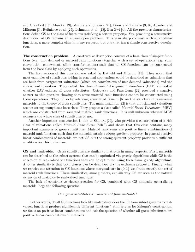
GS and matroids. Gross substitutes are similar to matroids in many respects. First, matroidscan be described as the subset systems that can be optimized via greedy algorithms while GS is thecollection of real-valued set functions that can be optimized using these same greedy algorithms.Another similarity is that both classes can be described via the exchange property. Finally, whenwe restrict our attention to GS functions where marginals are in {0, 1} we obtain exactly the set ofmatroid rank functions. These similarities, among others, explain why GS are seen as the naturalextension of matroids to real-valued functions.

The lack of constructive characterization for GS, combined with GS naturally generalizingmatroids, begs the following question.

Can gross substitutes be constructed from matroids?

In other words, do all GS functions look like matroids or does the lift from subset systems to real-valued functions produce significantly different functions? Similarly as for Shioura’s construction,we focus on positive linear combinations and ask the question of whether all gross substitutes arepositive linear combinations of matroids.

2

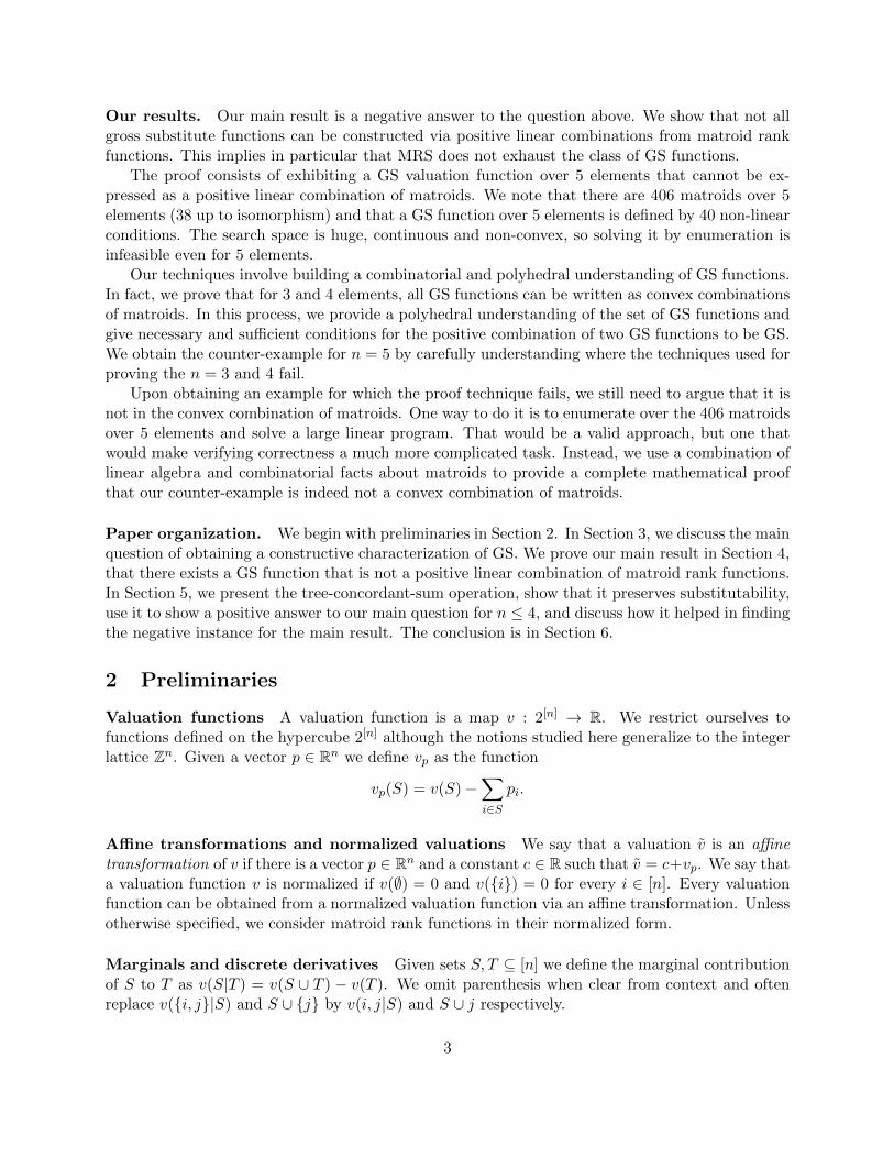
Our results. Our main result is a negative answer to the question above. We show that not allgross substitute functions can be constructed via positive linear combinations from matroid rankfunctions. This implies in particular that MRS does not exhaust the class of GS functions.

The proof consists of exhibiting a GS valuation function over 5 elements that cannot be ex-pressed as a positive linear combination of matroids. We note that there are 406 matroids over 5elements (38 up to isomorphism) and that a GS function over 5 elements is defined by 40 non-linearconditions. The search space is huge, continuous and non-convex, so solving it by enumeration isinfeasible even for 5 elements.

Our techniques involve building a combinatorial and polyhedral understanding of GS functions.In fact, we prove that for 3 and 4 elements, all GS functions can be written as convex combinationsof matroids. In this process, we provide a polyhedral understanding of the set of GS functions andgive necessary and sufficient conditions for the positive combination of two GS functions to be GS.We obtain the counter-example for n = 5 by carefully understanding where the techniques used forproving the n = 3 and 4 fail.

Upon obtaining an example for which the proof technique fails, we still need to argue that it isnot in the convex combination of matroids. One way to do it is to enumerate over the 406 matroidsover 5 elements and solve a large linear program. That would be a valid approach, but one thatwould make verifying correctness a much more complicated task. Instead, we use a combination oflinear algebra and combinatorial facts about matroids to provide a complete mathematical proofthat our counter-example is indeed not a convex combination of matroids.

Paper organization. We begin with preliminaries in Section 2. In Section 3, we discuss the mainquestion of obtaining a constructive characterization of GS. We prove our main result in Section 4,that there exists a GS function that is not a positive linear combination of matroid rank functions.In Section 5, we present the tree-concordant-sum operation, show that it preserves substitutability,use it to show a positive answer to our main question for n ≤ 4, and discuss how it helped in findingthe negative instance for the main result. The conclusion is in Section 6.

2 Preliminaries

Valuation functions A valuation function is a map v : 2[n] → R. We restrict ourselves tofunctions defined on the hypercube 2[n] although the notions studied here generalize to the integerlattice Zn. Given a vector p ∈ Rn we define vp as the function

vp(S) = v(S)−∑i∈S

pi.

Affine transformations and normalized valuations We say that a valuation v is an affinetransformation of v if there is a vector p ∈ Rn and a constant c ∈ R such that v = c+vp. We say thata valuation function v is normalized if v(∅) = 0 and v({i}) = 0 for every i ∈ [n]. Every valuationfunction can be obtained from a normalized valuation function via an affine transformation. Unlessotherwise specified, we consider matroid rank functions in their normalized form.

Marginals and discrete derivatives Given sets S, T ⊆ [n] we define the marginal contributionof S to T as v(S|T ) = v(S ∪ T ) − v(T ). We omit parenthesis when clear from context and oftenreplace v({i, j}|S) and S ∪ {j} by v(i, j|S) and S ∪ j respectively.

3

Given a function v : 2[n] → R and i ∈ [n] we define the derivative with respect to element i asthe function ∂iv : 2[n]\i → R where ∂iv(S) = v(S ∪ i) − v(S). The first derivative is simply themarginal v(i|S). Applying the operator twice we obtain the second derivative:

∂ijv(S) = ∂j [∂iv(S)] = ∂iv(S ∪ j)− ∂iv(S) = v(S ∪ ij)− v(S ∪ i)− v(S ∪ j) + v(S)

There is a nice economic interpretation of the second derivatives as a measure of the degree ofsubstitutability of two goods. ∂ijv(S) represents the difference between the value of the bundle{i, j} and sum of values of the two goods i and j separately. For example, if ∂ijv(S) = 0, it meansthat having good i does not affect the value for good j conditioned on having a bundle S.

Functions as vectors We often view valuation functions v : 2[n] → R as a vector in R2n withcoordinates indexed by S ⊆ [n]. This allows us to view a class of valuation functions as a subset ofR2n . We define the inner product between two valuations in the usual way:

〈v, w〉 =∑S⊆[n]

v(S)w(S).

2.1 Substitutability

There are several equivalent ways to define gross substitutes, often also called GS, discrete concavefunctions or simply substitutes. The definition that is most convenient to work with for our theoremsis the definition via discrete derivatives due to Reijnierse et al. [25] . The set Gn of gross substitutesis defined by:

Gn = {v : 2[n] → R; ∂ijv(S) ≤ max[∂ikv(S), ∂jkv(S)] ≤ 0, ∀S ⊆ [n], ∀i, j, k /∈ S}

We note that the definition does not require monotonicity.We also state some of the most common ways to define substitutes below. We refer to [24] for

a proof that they are equivalent to the definition above as well as other formulations.

• No price complementarity. In economics, substitutes was originally formulated as thecondition that an increase in price for a certain good, cannot decrease the demand for othergoods. Formally, given a vector p ∈ Rn, let D(v; p) = argmaxS⊆[n] vp(S) be the demandcorrespondence. Then v ∈ Gn iff for all vectors p ≤ p′ and S ∈ D(v; p) there is S′ ∈ D(v; p′)such that S ∩ {j; pj = p′j} ⊆ S′.

• Discrete concavity. In discrete mathematics, substitutes are a natural notion of concavityfor functions defined in the hypercube. We say that a function over the reals f : Rn → R isconcave if for every vector p ∈ Rn, every local minimum of fp(x) = f(x) −

∑i pixi is also a

global minimum1. This definition naturally extends to the hypercube: v ∈ Gn iff for everyp ∈ Rn, if S is a local minimum of vp, i.e.

vp(S) ≥ vp(S ∪ i) vp(S) ≥ vp(S \ j) vp(S) ≥ vp(S ∪ i \ j),∀i /∈ S, j ∈ S

then S is also a global minimum, i.e. S ∈ D(v; p).

1That is perhaps not the most common definition of concavity but it is completely equivalent to the conditionf(tx + (1− t)y) ≥ tf(x) + (1− t)f(y),∀t ∈ [0, 1].

4

• Matroidality. Substitutes can also be defined in terms of greedy algorithms: v ∈ Gn iff forevery p ∈ Rn, the greedy algorithm always computes the maximum of vp, i.e., if we start withS = ∅ and keeps adding the element i ∈ argmaxi vp(i|S) with largest marginal contributionwhile it is positive, we obtain S ∈ D(v; p).

2.2 Matroids

Many of those definitions strikingly resemble the definition of matroids. In fact some of the earlyappearances of gross substitutes were attempts to generalize matroids from collections of subsetsto real-valued functions. Dress and Terhalle [9, 8] called their definition matroidal maps and Dressand Wenzel called their notion valuated matroids.

A subset collection over [n] is simply a subset M ⊆ 2[n]. This subset collection is a matroid ifit satisfies one of the following equivalent properties:

• Greedy optimization. The collection M is a matroid if for every vector p ∈ Rn, the setS ∈ M maximizing

∑i∈S pi can be obtained by the greedy algorithm that starts with the

empty set S = ∅ and keeps adding i ∈ argmaxi;S∪i∈M pi to S while pi is positive.

• Exchange property. We say that collection M is a matroid if T ⊆ S ∈ M then T ∈ Mand for every S, T ∈M with |S| < |T |, there is i ∈ T \ S such that S ∪ i ∈M.

Given any subset system M, we can define its rank function rM : 2[n] → Z+ as rM(S) =max{|T | ;T ⊆ S and T ∈M}. This allows us to define the set of matroid rank functions as:

Mn = {rM;M is matroid over [n]}

When we translate the subset system M to a rank function rM, the exchange property becomesexactly the discrete differential equation in the definition of Gn. This observation implies thatmatroid rank functions are exactly the gross substitutes functions with {0, 1}-marginals:

Mn = {v ∈ Gn; v(∅) = 0; ∂iv(S) ∈ {0, 1},∀S ⊆ [n], i /∈ S}

For completeness, we provide a proof of this result in Theorem 19 in the appendix.

2.3 Relation between classes of functions

Another class that is important for us is submodular functions:

Sn = {v : 2[n] → R; ∂ijv(S) ≤ 0,∀S ⊆ [n], i, j /∈ S}

The following relation between the classes hold: Mn ⊆ Gn ⊆ Sn. The classes Gn and Sn are definedin terms of second order discrete derivatives, which are invariant under affine transformations, i.e,if v is obtained from v via an affine transformation then ∂ijv(S) = ∂ij v(S). In particular this meansthat gross substitutes is invariant under affine transformations. If we want to understand Gn it isenough to understand the class Gn

0 of normalized gross substitutes:

Gn0 = {v ∈ Gn; v(∅) = v(i) = 0, ∀i ∈ [n]}

5

since we can describe Gn = Gn0 + En where En is the class of affine valuations functions:

En = {v : 2[n] → R; v(S) = c+∑

i∈S pi; c, pi ∈ R}

It will also be convenient to define the notion of normalized matroid rank functions:

Mn0 = {v : 2[n] → R;∃M matroid s.t. v(S) = rM(S)−

∑i∈S rM(i)},

which are exactly the normalized gross substitutes functions Gn0 with {−1, 0}-marginals.

3 What are the building blocks of Substitutes ?

A major open question in the theory of gross substitutes is how to find a constructive descriptionof the class. A constructive description has two parts: a base class of simpler functions and a setof operations that allow us to build complex functions from simpler ones. There are a number ofoperations that are known to preserve substitutability. We mention the two that are most relevantfor this paper here and discuss additional operations in Section 6.

• Affine transformations. If v : 2[n] → R satisfies gross substitutes and p ∈ R[n] is avector and u0 ∈ R then we can build the affine transformation v : 2[n] → R as v(S) =v(S) +

∑i∈S pi + u0.

• Strong Quotient Sum [29]. Give two valuations v, w : 2[n] → R and α1, α2 ≥ 0 , we saythat v is a strong quotient of w if v(S|T ) ≤ w(S|T ) for all S, T ⊆ [n]. Given two valuations vand w such that v is a strong quotient of w and w is a matroid rank function, we define thestrong quotient sum v : 2[n] → R as v(S) = α1v(S) + α2w(S).

Those operations are known to preserve gross substitutability. A major open question is whetherall substitutes can be built from matroid rank functions using those operations (or perhaps alarger class of simpler operations). We focus here on affine transformations and positive linearcombinations (which is a strict generalization of the strong quotient sum operation).

Main Question. Are all gross substitutes positive combinations of matroid rank functions moduloan affine transformation? Formally, given v ∈ Gn, is there an affine transformation v ∈ Gn,matroid rank functions ri ∈Mn and positive constants αi ∈ R+ such that:

v =∑

i αiri.

An equivalent way to ask this question is via the normalized classes: this allows us to ignorethe affine transformations. Given v ∈ Gn

0 , are there ri ∈Mn0 and αi ≥ 0 such that v =

∑i αiri?

3.1 Building blocks for submodular functions

Before we go into our results, we would like to mention a simple constructive description forsubmodular functions Sn having the set of matroid rank functions as base. This will serve asa warm up for the study of substitute valuations. Besides affine transformations, the followingoperations preserve submodularity:2

2We note that even though positive linear combination and item grouping preserve submodularity, neither of thempreserves substitutability in general.

6

• Positive linear combination. If v1, v2 : 2[n] → R are submodular and α1, α2 ≥ 0 thenv = α1v1 + α2v2 is also submodular.

• Item grouping. If v : 2[n] → R is submodular and S1, . . . , Sk is a partition of [n] then thefunction w : 2[k] → R defined as w(T ) = v(∪t∈TSt) is also submodular.

It turns out those operations are sufficient to build any submodular function starting from theset of matroid rank functions. A proof is provided in Appendix B.

Theorem 1. Any submodular function can be obtained starting from the set of matroid rank func-tions and applying the operations of affine transformations, positive linear combination and itemgrouping.

4 GS is not in the cone of matroids

In this section, we exhibit a specific GS function and show that it cannot be expressed as a positivelinear combination of matroid rank functions. This section is devoted to a (non-computational)proof of that fact. We defer to Section 5 a discussion on how we found such function.

At a high level, the analysis uses duality and Farkas’ lemma. Farkas’s conditions require theexistence of a certificate whose inner product with all matroid rank functions has non-negative signand the inner product with the candidate function is strictly negative (Section 4.1). The core of theproof consists in showing in a non-computational manner that the certificate satisfies the desiredconditions (Section 4.2). This is done with a simple lemma about the local structure of matroidrank functions and a non-trivial partition of the collection of sets into local groups that can beanalyzed individually with that lemma.

4.1 The GS function and the certificate

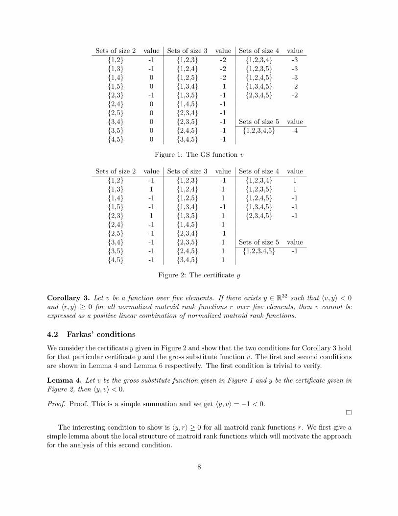
The GS function that we consider for the remaining in this section is over five elements [5] ={1, 2, 3, 4, 5}. This function v is described in its normalized form3 in Figure 1. Since the functionis normalized, it is enough to define it for |S| ≥ 2. Checking that the function satisfies the GSconditions (v ∈ G5

0) amounts to checking the inequalities: ∂ijv(S) ≤ max[∂ikv(S), ∂kjv(S)] ≤ 0 forall S ⊆ [5]. There are 40 such inequalities. It is a tedious but short verification, which can be foundin Appendix C.1.

Now that we established that v ∈ G50, we want to prove that there do not exist (normalized)

matroid rank functions4 ri ∈M50 and αi ≥ 0 such that v =

∑ni=1 αiri.

Lemma 2 (Farkas’ Lemma). Let M ∈ Rm×n and v ∈ Rm. Then exactly one of the following twostatements is true:

• There exists α ∈ Rn such that v = Mα and α ≥ 0

• There exists y ∈ Rm such that Mᵀy ≥ 0 and 〈v, y〉 < 0.

We immediately obtain the following corollary which gives two conditions such that, if satisfied,we obtain the desired negative result.

3Recall from Section 2 that a valuation function is normalized if v(∅) = v(i) = 0 for all i ∈ [5].4Recall the definition of a normalized matroid rank function in Section 2.3.

7

Sets of size 2 value Sets of size 3 value Sets of size 4 value

{1,2} -1 {1,2,3} -2 {1,2,3,4} -3{1,3} -1 {1,2,4} -2 {1,2,3,5} -3{1,4} 0 {1,2,5} -2 {1,2,4,5} -3{1,5} 0 {1,3,4} -1 {1,3,4,5} -2{2,3} -1 {1,3,5} -1 {2,3,4,5} -2{2,4} 0 {1,4,5} -1{2,5} 0 {2,3,4} -1{3,4} 0 {2,3,5} -1 Sets of size 5 value{3,5} 0 {2,4,5} -1 {1,2,3,4,5} -4{4,5} 0 {3,4,5} -1

Figure 1: The GS function v

Sets of size 2 value Sets of size 3 value Sets of size 4 value

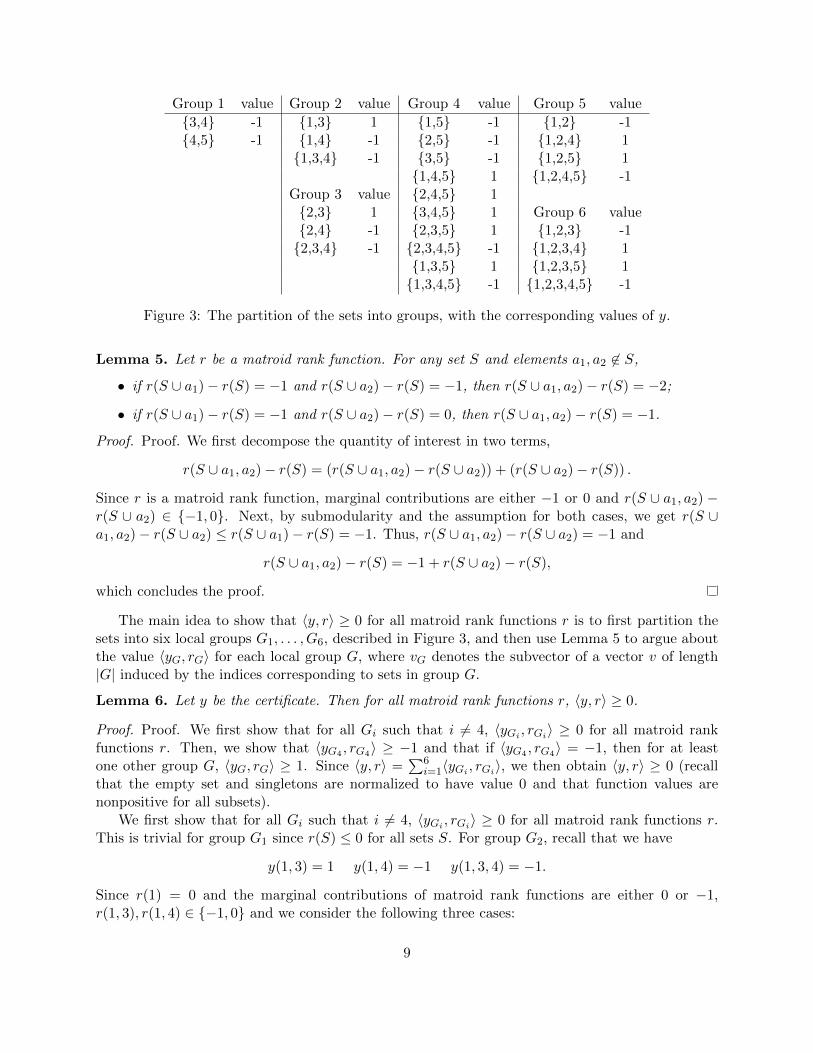
{1,2} -1 {1,2,3} -1 {1,2,3,4} 1{1,3} 1 {1,2,4} 1 {1,2,3,5} 1{1,4} -1 {1,2,5} 1 {1,2,4,5} -1{1,5} -1 {1,3,4} -1 {1,3,4,5} -1{2,3} 1 {1,3,5} 1 {2,3,4,5} -1{2,4} -1 {1,4,5} 1{2,5} -1 {2,3,4} -1{3,4} -1 {2,3,5} 1 Sets of size 5 value{3,5} -1 {2,4,5} 1 {1,2,3,4,5} -1{4,5} -1 {3,4,5} 1

Figure 2: The certificate y

Corollary 3. Let v be a function over five elements. If there exists y ∈ R32 such that 〈v, y〉 < 0and 〈r, y〉 ≥ 0 for all normalized matroid rank functions r over five elements, then v cannot beexpressed as a positive linear combination of normalized matroid rank functions.

4.2 Farkas’ conditions

We consider the certificate y given in Figure 2 and show that the two conditions for Corollary 3 holdfor that particular certificate y and the gross substitute function v. The first and second conditionsare shown in Lemma 4 and Lemma 6 respectively. The first condition is trivial to verify.

Lemma 4. Let v be the gross substitute function given in Figure 1 and y be the certificate given inFigure 2, then 〈y, v〉 < 0.

Proof. Proof. This is a simple summation and we get 〈y, v〉 = −1 < 0.

The interesting condition to show is 〈y, r〉 ≥ 0 for all matroid rank functions r. We first give asimple lemma about the local structure of matroid rank functions which will motivate the approachfor the analysis of this second condition.

8

Group 1 value Group 2 value Group 4 value Group 5 value

{3,4} -1 {1,3} 1 {1,5} -1 {1,2} -1{4,5} -1 {1,4} -1 {2,5} -1 {1,2,4} 1

{1,3,4} -1 {3,5} -1 {1,2,5} 1{1,4,5} 1 {1,2,4,5} -1

Group 3 value {2,4,5} 1{2,3} 1 {3,4,5} 1 Group 6 value{2,4} -1 {2,3,5} 1 {1,2,3} -1{2,3,4} -1 {2,3,4,5} -1 {1,2,3,4} 1

{1,3,5} 1 {1,2,3,5} 1{1,3,4,5} -1 {1,2,3,4,5} -1

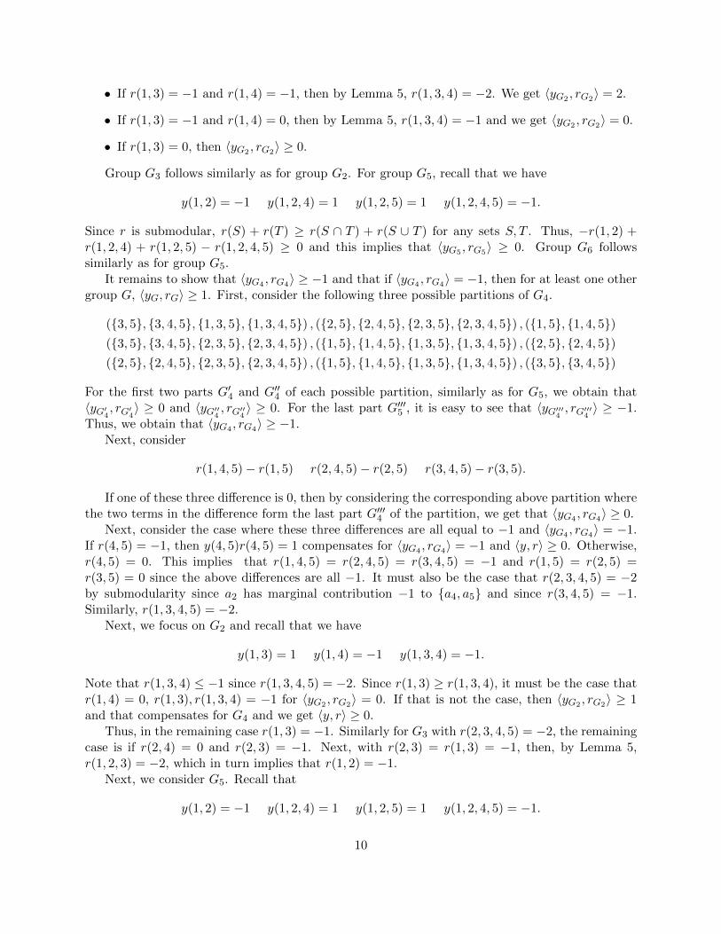
Figure 3: The partition of the sets into groups, with the corresponding values of y.

Lemma 5. Let r be a matroid rank function. For any set S and elements a1, a2 6∈ S,

• if r(S ∪ a1)− r(S) = −1 and r(S ∪ a2)− r(S) = −1, then r(S ∪ a1, a2)− r(S) = −2;

• if r(S ∪ a1)− r(S) = −1 and r(S ∪ a2)− r(S) = 0, then r(S ∪ a1, a2)− r(S) = −1.

Proof. Proof. We first decompose the quantity of interest in two terms,

r(S ∪ a1, a2)− r(S) = (r(S ∪ a1, a2)− r(S ∪ a2)) + (r(S ∪ a2)− r(S)) .

Since r is a matroid rank function, marginal contributions are either −1 or 0 and r(S ∪ a1, a2) −r(S ∪ a2) ∈ {−1, 0}. Next, by submodularity and the assumption for both cases, we get r(S ∪a1, a2)− r(S ∪ a2) ≤ r(S ∪ a1)− r(S) = −1. Thus, r(S ∪ a1, a2)− r(S ∪ a2) = −1 and

r(S ∪ a1, a2)− r(S) = −1 + r(S ∪ a2)− r(S),

which concludes the proof.

The main idea to show that 〈y, r〉 ≥ 0 for all matroid rank functions r is to first partition thesets into six local groups G1, . . . , G6, described in Figure 3, and then use Lemma 5 to argue aboutthe value 〈yG, rG〉 for each local group G, where vG denotes the subvector of a vector v of length|G| induced by the indices corresponding to sets in group G.

Lemma 6. Let y be the certificate. Then for all matroid rank functions r, 〈y, r〉 ≥ 0.

Proof. Proof. We first show that for all Gi such that i 6= 4, 〈yGi , rGi〉 ≥ 0 for all matroid rankfunctions r. Then, we show that 〈yG4 , rG4〉 ≥ −1 and that if 〈yG4 , rG4〉 = −1, then for at leastone other group G, 〈yG, rG〉 ≥ 1. Since 〈y, r〉 =

∑6i=1〈yGi , rGi〉, we then obtain 〈y, r〉 ≥ 0 (recall

that the empty set and singletons are normalized to have value 0 and that function values arenonpositive for all subsets).

We first show that for all Gi such that i 6= 4, 〈yGi , rGi〉 ≥ 0 for all matroid rank functions r.This is trivial for group G1 since r(S) ≤ 0 for all sets S. For group G2, recall that we have

y(1, 3) = 1 y(1, 4) = −1 y(1, 3, 4) = −1.

Since r(1) = 0 and the marginal contributions of matroid rank functions are either 0 or −1,r(1, 3), r(1, 4) ∈ {−1, 0} and we consider the following three cases:

9

• If r(1, 3) = −1 and r(1, 4) = −1, then by Lemma 5, r(1, 3, 4) = −2. We get 〈yG2 , rG2〉 = 2.

• If r(1, 3) = −1 and r(1, 4) = 0, then by Lemma 5, r(1, 3, 4) = −1 and we get 〈yG2 , rG2〉 = 0.

• If r(1, 3) = 0, then 〈yG2 , rG2〉 ≥ 0.

Group G3 follows similarly as for group G2. For group G5, recall that we have

y(1, 2) = −1 y(1, 2, 4) = 1 y(1, 2, 5) = 1 y(1, 2, 4, 5) = −1.

Since r is submodular, r(S) + r(T ) ≥ r(S ∩ T ) + r(S ∪ T ) for any sets S, T . Thus, −r(1, 2) +r(1, 2, 4) + r(1, 2, 5) − r(1, 2, 4, 5) ≥ 0 and this implies that 〈yG5 , rG5〉 ≥ 0. Group G6 followssimilarly as for group G5.

It remains to show that 〈yG4 , rG4〉 ≥ −1 and that if 〈yG4 , rG4〉 = −1, then for at least one othergroup G, 〈yG, rG〉 ≥ 1. First, consider the following three possible partitions of G4.

({3, 5}, {3, 4, 5}, {1, 3, 5}, {1, 3, 4, 5}) , ({2, 5}, {2, 4, 5}, {2, 3, 5}, {2, 3, 4, 5}) , ({1, 5}, {1, 4, 5})({3, 5}, {3, 4, 5}, {2, 3, 5}, {2, 3, 4, 5}) , ({1, 5}, {1, 4, 5}, {1, 3, 5}, {1, 3, 4, 5}) , ({2, 5}, {2, 4, 5})({2, 5}, {2, 4, 5}, {2, 3, 5}, {2, 3, 4, 5}) , ({1, 5}, {1, 4, 5}, {1, 3, 5}, {1, 3, 4, 5}) , ({3, 5}, {3, 4, 5})

For the first two parts G′4 and G′′4 of each possible partition, similarly as for G5, we obtain that〈yG′4 , rG′4〉 ≥ 0 and 〈yG′′4 , rG′′4 〉 ≥ 0. For the last part G′′′5 , it is easy to see that 〈yG′′′4 , rG′′′4 〉 ≥ −1.Thus, we obtain that 〈yG4 , rG4〉 ≥ −1.

Next, consider

r(1, 4, 5)− r(1, 5) r(2, 4, 5)− r(2, 5) r(3, 4, 5)− r(3, 5).

If one of these three difference is 0, then by considering the corresponding above partition wherethe two terms in the difference form the last part G′′′4 of the partition, we get that 〈yG4 , rG4〉 ≥ 0.

Next, consider the case where these three differences are all equal to −1 and 〈yG4 , rG4〉 = −1.If r(4, 5) = −1, then y(4, 5)r(4, 5) = 1 compensates for 〈yG4 , rG4〉 = −1 and 〈y, r〉 ≥ 0. Otherwise,r(4, 5) = 0. This implies that r(1, 4, 5) = r(2, 4, 5) = r(3, 4, 5) = −1 and r(1, 5) = r(2, 5) =r(3, 5) = 0 since the above differences are all −1. It must also be the case that r(2, 3, 4, 5) = −2by submodularity since a2 has marginal contribution −1 to {a4, a5} and since r(3, 4, 5) = −1.Similarly, r(1, 3, 4, 5) = −2.

Next, we focus on G2 and recall that we have

y(1, 3) = 1 y(1, 4) = −1 y(1, 3, 4) = −1.

Note that r(1, 3, 4) ≤ −1 since r(1, 3, 4, 5) = −2. Since r(1, 3) ≥ r(1, 3, 4), it must be the case thatr(1, 4) = 0, r(1, 3), r(1, 3, 4) = −1 for 〈yG2 , rG2〉 = 0. If that is not the case, then 〈yG2 , rG2〉 ≥ 1and that compensates for G4 and we get 〈y, r〉 ≥ 0.

Thus, in the remaining case r(1, 3) = −1. Similarly for G3 with r(2, 3, 4, 5) = −2, the remainingcase is if r(2, 4) = 0 and r(2, 3) = −1. Next, with r(2, 3) = r(1, 3) = −1, then, by Lemma 5,r(1, 2, 3) = −2, which in turn implies that r(1, 2) = −1.

Next, we consider G5. Recall that

y(1, 2) = −1 y(1, 2, 4) = 1 y(1, 2, 5) = 1 y(1, 2, 4, 5) = −1.

10

Since r(4, 5) = 0, r(1, 4, 5) = −1 and r(2, 4, 5) = −1, by Lemma 5, r(1, 2, 4, 5) = −2. Ifr(1, 2, 5), r(1, 2, 4) = −1, then with r(1, 2) = −1, 〈yG5 , rG5〉 ≥ 1 and we are done. Otherwise,r(1, 2, 5) or r(1, 2, 4) is equal to −2. But this is impossible since we are in a case where r(1, 5) = 0and r(1, 4) = 0. Thus, if 〈yG4 , rG4〉 = −1, then for at least one other group G, 〈yG, rG〉 ≥ 1 and weget 〈y, r〉 ≥ 0.

Combining Corollary 3, Lemma 4 and Lemma 6, we obtain the main result.

Theorem 7. The gross substitute function v cannot be expressed as a positive linear combinationof normalized matroid rank functions. In particular, no affine transformation of v can be expressedas a positive linear combination of matroid rank functions.

In particular, this implies that the strong quotient sum and tree-concordant-sum operations arenot sufficient to construct all gross substitutes from matroid rank functions and that MRS valuationsdo not exhaust gross substitutes. We note that even though v is non-monotone, the main resultholds for monotone gross substitute functions since there exists some affine transformation of v thatis monotone. We also extend the negative result from matroid rank functions to weighted matroidrank functions. This follows from the fact that weighted matroid rank functions can be expressedas a positive linear combination of unweighted matroid rank functions, which was proven in [29]and we give a proof in Appendix C for completeness as Lemma 22.

Corollary 8. No affine transformation of function v can be expressed as a positive linear combi-nation of weighted matroid rank functions.

5 The Tree-Concordant-Sum Operation

In this section, we define the notion of a tree representation which abstracts the combinatorialstructure of tree-form Hessians of Hirai and Murota [15]. We first show that this representation hasthe following nice property: the condition that two functions have such a tree representation thatis compatible is necessary and sufficient for the summation operation to preserve substitutability.We call this new operation preserving substitutability tree-concordant-sum and show that it alsoprovides a polyhedral characterization of gross substitutes.

We then use this representation to give a positive answer to our main question for n ≤ 4: a GSover at most 4 elements can be written as a positive linear combination of matroid rank functions.This implies that at least 5 elements are necessary to obtain the negative answer from the previoussection.

Finally, we discuss how the polyhedral understanding of gross substitutes based on this treerepresentation combined with computational techniques led to the discovery of the counterexamplefor n = 5.

5.1 Substitution Trees

The tree representation of GS is best explained using the discrete derivative property introducedin Section 2. Since it will be convenient to work with non-negative numbers, we introduce thenotation:

∆Sij(v) = −∂ijv(S)

11

omitting v when clear from context. In this notation, we can write the GS condition as:

∆Sij ≥ min(∆S

ik,∆Sjk) ≥ 0

If we permute the identities of i, j, k such that the symbols are sorted, we have the following triangleproperty: ∆S

ij = ∆Sik ≤ ∆S

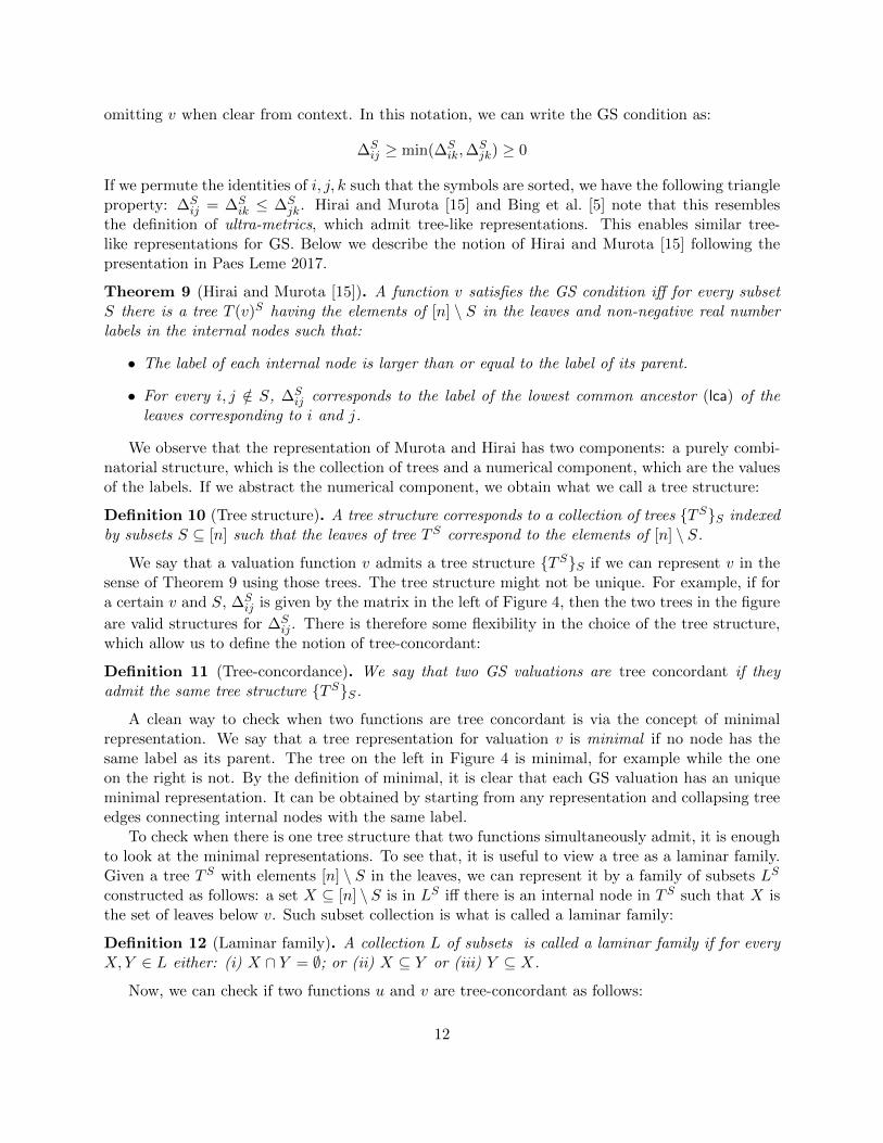
jk. Hirai and Murota [15] and Bing et al. [5] note that this resemblesthe definition of ultra-metrics, which admit tree-like representations. This enables similar tree-like representations for GS. Below we describe the notion of Hirai and Murota [15] following thepresentation in Paes Leme 2017.

Theorem 9 (Hirai and Murota [15]). A function v satisfies the GS condition iff for every subsetS there is a tree T (v)S having the elements of [n] \ S in the leaves and non-negative real numberlabels in the internal nodes such that:

• The label of each internal node is larger than or equal to the label of its parent.

• For every i, j /∈ S, ∆Sij corresponds to the label of the lowest common ancestor (lca) of the

leaves corresponding to i and j.

We observe that the representation of Murota and Hirai has two components: a purely combi-natorial structure, which is the collection of trees and a numerical component, which are the valuesof the labels. If we abstract the numerical component, we obtain what we call a tree structure:

Definition 10 (Tree structure). A tree structure corresponds to a collection of trees {TS}S indexedby subsets S ⊆ [n] such that the leaves of tree TS correspond to the elements of [n] \ S.

We say that a valuation function v admits a tree structure {TS}S if we can represent v in thesense of Theorem 9 using those trees. The tree structure might not be unique. For example, if fora certain v and S, ∆S

ij is given by the matrix in the left of Figure 4, then the two trees in the figure

are valid structures for ∆Sij . There is therefore some flexibility in the choice of the tree structure,

which allow us to define the notion of tree-concordant:

Definition 11 (Tree-concordance). We say that two GS valuations are tree concordant if theyadmit the same tree structure {TS}S.

A clean way to check when two functions are tree concordant is via the concept of minimalrepresentation. We say that a tree representation for valuation v is minimal if no node has thesame label as its parent. The tree on the left in Figure 4 is minimal, for example while the oneon the right is not. By the definition of minimal, it is clear that each GS valuation has an uniqueminimal representation. It can be obtained by starting from any representation and collapsing treeedges connecting internal nodes with the same label.

To check when there is one tree structure that two functions simultaneously admit, it is enoughto look at the minimal representations. To see that, it is useful to view a tree as a laminar family.Given a tree TS with elements [n] \ S in the leaves, we can represent it by a family of subsets LS

constructed as follows: a set X ⊆ [n] \ S is in LS iff there is an internal node in TS such that X isthe set of leaves below v. Such subset collection is what is called a laminar family:

Definition 12 (Laminar family). A collection L of subsets is called a laminar family if for everyX,Y ∈ L either: (i) X ∩ Y = ∅; or (ii) X ⊆ Y or (iii) Y ⊆ X.

Now, we can check if two functions u and v are tree-concordant as follows:

12

∗ 2 1 1 1

2 ∗ 1 1 1

1 1 ∗ 3 3

1 1 3 ∗ 3

1 1 3 3 ∗

1

2

a b

3

c d e

1

2

a b

3

3

c d

e

Figure 4: Two valid tree representations for the same matrix [∆Sij ]ij .

Lemma 13. If u and v are GS functions and {TS(u)} and {TS(v)} are its minimal tree structuresand {LS(u)} and {LS(v)} are its corresponding laminar family representations, then u and v aretree concordant iff for every S, LS(u) ∪ LS(v) is also a laminar family.

The proof is straightforward from definitions and the fact that there is natural one-to-onemapping between trees and laminar families. What is interesting about tree concordance is that itprovides necessary and sufficient conditions for the sum of two GS functions to be GS:

Theorem 14. Let u and v be two gross substitute functions. The function u+v is a gross substitutefunction if and only if u and v are tree-concordant.

Proof. Proof. We first show that if u and v are tree-concordant, then u + v is a gross-substitute.Consider the tree representation T that has the structure of u and v, which is identical since theyare tree-concordant, but with numerical values at each internal node that is the sum of the valuesat that node for u and v. Since second order derivatives are linear:

∆Sij(u+ v) = ∆S

ij(u) + ∆Sij(v)

and it clearly admits the same tree structure T , so by Theorem 9, u+ v is in GS.Next, we show that if u and v are not tree-concordant, then u + v is not a gross substitute

function. Assume u and v are not tree-concordant then by Lemma 13 there is a set S such thatfor the laminar representations LS(u) and LS(v) there are sets with non-trivial intersection, i.e.,there are X ∈ LS(u) and Y ∈ LS(v) such that we can find i ∈ X \ Y , j ∈ X ∩ Y and k ∈ Y \X.Therefore:

∆Sij(u) > ∆S

ik(u) = ∆Skj(u)

∆Sij(v) = ∆S

ik(v) < ∆Skj(v)

therefore, it must be the case that:

∆Sik(u+ v) < min[∆S

ij(u+ v),∆Skj(u+ v)]

which is a violation of gross substitutability.

Since it is a necessary and sufficient condition, this includes the strong-quotient-sum propertyin [29] as a special case:

Corollary 15. If a GS function u and a matroid rank function v satisfy the strong-quotient-sumproperty, then they are tree-concordant.

13

5.2 Polyhedral description of Gn

The concept of tree structure and tree concordance provide a good tool for describing the geometryof Gn. Viewing valuations as vectors in R2n , we can view Gn as a subset of that space. Lehmann,Lehmann and Nisan [18] observe that the set is a non-convex and has zero measure.

The concepts developed earlier in this section allow us to decompose the space in finitely manyconvex cones. Since a tree structure is a finite combinatorial object, there are finitely many suchstructures. Fix a tree structure {TS}S and consider the subset of Gn with functions that admit{TS}S . All functions in this subset are tree concordant, so the set is closed under positive linearcombination, forming a convex cone.

What we would like to do next is to understand how those cones look like. For that we willfix a tree structure and assign labels to internal nodes. The labels must be non-negative and thelabel of a node cannot be smaller than the label of its parent, but those conditions alone are notsufficient for the existence of a valuation function producing those ∆S

ij . An extra condition that is

required is what we call integrability5:

∆S+kij −∆S

ij = ∆S+jik −∆S

ik = ∆S+ijk −∆S

jk (Int)

Lemma 16 (Integrability). Given values ∆Sij for all i, j, S such that i, j 6∈ S, there is a valuation

v such that ∂ijv(S) = −∆Sij if and only if the integrability conditions (Int) hold.

In Appendix D we provide a discussion on integrability conditions for discrete functions. Thelemma above follows directly from Lemma 24 in the appendix.

Since the symbols ∆Sij have a special tree-form for gross substitutes, it is convenient to re-write

the integrability conditions in the following form. We simplify the notation for S ∪ {i} with S + ifor the remainder of the paper.

Lemma 17. An assignment of labels to the internal nodes of a tree structure corresponds to arepresentation of GS function if and only if the following condition holds for every S ⊆ [n] andi, j, k /∈ S:

if ∆Sik = ∆S

jk = ∆Sij − α, for some α ≥ 0

then ∆S+jik = ∆S+i

jk = ∆S+kij − α

The following corollary (which is a rephrasing of Corollary 25 in the appendix) shows howto explicitly reconstruct a function from second order derivatives. We denote by S<i the set ofelements smaller than i according to their label, i.e., S<i = {j : j < i}.

Corollary 18. Given ∆Sij satisfying the integrability conditions (Int), the unique normalized func-

tion such that ∂ijv(S) = −∆Sij is given by:

v(S) = −∑

i,j∈S;i<j

∆S<i

ij

In particular, all the functions such that ∂ijv(S) = −∆Sij are affine transformations of the function

defined above.

5We thank Kazuo Murota for his suggestion on a earlier version of this manuscript to phrase this analysis in termsof integrability condition.

14

m1∅:

m2

a b

c

m3{a}:

b c

m4{b}:

a c

m5{c}:

a b

Figure 5: The tree structure for functions in G3.

5.3 Representations of G

Using the tree representation of gross substitutes, we provide a constructive characterization ofgross substitutes Gn for n ≤ 4 from matroids. Given a matroid M we denote its rank by r[M].We denote the uniform matroid of rank i over j elements by U i

j .Given two functions v and v we say that they are equivalent (up to affine transformations) if

v − v ∈ En. Given a normalized valuation v ∈ Gn0 , we will often associate it with the equivalent

function v(S) = v(S) + |S|. Often, a normalized matroid rank function v is easier to recognize inits v form.

Moreover, we write X ' Y to denote a linear isomorphism between two sets, i.e., if there is alinear bijection L such that L(X) = Y .

5.3.1 Description of G2

For n = 2, the only constraint is ∆∅1,2 ≥ 0 so:

G20 = {(v(∅) = 0, v(1) = 0, v(2) = 0, v(12)); v(12) ≤ 0} ' R+.

Thus, v = (0, 0, 0,−1) is a representative of the class G20 and v = (0, 1, 1, 1), which is the rank

function r[U12 ] of the uniform matroid of rank 1 over 2 elements, is a representative of the class G2.

Since E2 = (1, 1, 1, 1) · R + (0, 1, 0, 1) · R + (0, 0, 1, 1) · R ' R3, we have:

G2 = E2 + r[U12 ] · R+ ' R3 × R+.

The set G2 is not very interesting since the set of gross substitutes on 2 variables is the same asthe set of submodular functions on 2 variables, which is known to be a convex set.

5.3.2 Description of G3

The set of gross substitutes on 3 items is more interesting since it is not convex. We name the items{a, b, c}. For every v ∈ G3

0 and up to the renaming of the elements, there is only one possibility forthe substitution tree associated to the empty set, which is depicted in Figure 5. For each singletonset, there is also only one possible substitution tree. Applying Lemma 17 that is required to obtaina well-defined function, with S = ∅, we obtain the following additional necessary and sufficientconstraint for the labels in Figure 5:

m3 = m4 = m5 − (m2 −m1).

15

We write m1 = x, m2−m1 = y (recall m2 ≥ m1) and m3 = z, so we can parametrize the spaceof feasible m = (m1,m2,m3,m4,m5) by:

(x, y, z) ∈ R3+ 7→ m = (x, x+ y, z, z, y + z)

In other words, the space of feasible values of m is a cone generated by the following vectors:(1, 1, 0, 0, 0), (0, 0, 1, 1, 1), (0, 1, 0, 0, 1). It is particularly interesting to see which valuations theycorrespond to.

Vector (1, 1, 0, 0, 0) By solving the equation to obtain v from second derivatives ∆ (Corollary18), we obtain the valuation v ∈ G3

0 such that v(ab) = v(bc) = v(ac) = −1 and v(abc) = −2. Thus,v(S) = v(S) + |S| = 1 for all S 6= ∅, which is the rank function r[U1

3 ].

Vector (0, 0, 1, 1, 1) Solving the equations for v we obtain v(ab) = v(bc) = v(ac) = 0 and v(abc) =−1, so v(S) = min{|S| , 2} which is r[U2

3 ].

Vector (0, 1, 0, 0, 1) More interestingly, by solving for v we obtain: v(ac) = v(bc) = 0 and v(ab) =v(abc) = −1, so v is such that the singletons have value 1, v(ab) = 1 and v(bc) = v(ac) = v(abc) = 2.This is the rank function of the graphical matroid associated with the following graph:

b

ac

We note that when we describe a matroid in terms of a graph in this document we refer tothe matroid where the ground set are the edges of the graph and a set is independent if thecorresponding edges do not form a cycle. Call the rank of this matroid r[M((ab)c)]. Therefore, theset of functions in G3 associated with the depicted ∅-tree is given by:

E3 + r[U13 ] · R+ + r[U2

3 ] · R+ + r[M((ab)c)] · R+

Since all the ∅-trees are symmetric, then all the gross substitute functions over 3 elements areof the form:

G3 = E3 + r[U13 ] · R+ + r[U2

3 ] · R+ +(r[M((ab)c)] · R+ ∪ r[M((ac)b)] · R+ ∪ r[M((bc)a)] · R+

)5.3.3 Description of G4

The description of G4 follows similarly as for G3, but with more cases. It is deferred to Appendix E.

5.4 Finding the counterexample

The main idea used to find counterexample v is to exhibit a specific tree structure over 5 elementsthat is complex enough so that, unlike for n = 1, 2, 3, and 4, node labels cannot be decomposedinto binary valued vectors which satisfy the integrability condition. We will try to mimic the sameproof used for G3 and G4 and find a set of trees for which the same proof technique cannot beextended.

Consider the tree defined in Figure 6. We can apply the integrability conditions (Int) to obtainthe following relations among the labels:

16

m1∅:

m2

1, 2, 3

4, 5

m3{5}:

m4

1, 2

3, 4

m5{1}:

m6

2, 4, 5

3

Figure 6: The key part of the tree structure for the counterexample.

• m3 −m5 = m2 −m1 ≥ 0 from (Int) with S = ∅ and (i, j, k) = (1, 3, 5),

• m6 −m3 = m1 −m1 = 0 from (Int) with S = ∅ and (i, j, k) = (1, 4, 5),

• m4 −m6 = m2 −m1 ≥ 0 from (Int) with S = ∅ and (i, j, k) = (1, 2, 5).

Consider a function that satisfies that tree structure and has m2 −m1 = ∆ > 0, then m4 =m6 + ∆ = m3 + ∆ = m5 + 2∆. Therefore, any parametrization of the space of functions sharingthose trees obtained by the same method as used for G3 and G4 will have a non-binary coefficientand hence does not decompose the space in combinations of matroid rank functions.

This is yet not a proof, since we do not know yet if there is GS functions with that treestructure and if there is a parametrization obtained by other methods that decomposes the space.Next, we complete this tree description and (computationally) solve a linear program to find afunction satisfying that tree structure. Once we get a candidate functions that is the output ofthis program, we write a second program that tries to write it as a convex combination of matroidrank functions by explicitly enumerating over the set of all matroid rank functions and creating onevariable for each in the linear program. Next, we verify that the program is infeasible and obtain aFarkas’ type certificate. Finally, since we do not want to rely on the correctness of the enumerationand the computational steps, we give a human readable proof.

6 Conclusion

The class of gross substitutes is a well-studied family of valuation functions that has many differentcharacterizations, but for which we do not know a constructive description. Our main resultshows that gross substitutes cannot be constructed via positive linear combinations of matroid rankfunctions. We also give a new operation, called tree-concordant-sum, which provides a necessaryand sufficient condition for the sum operation to preserve substitutability and which is used to findthe counterexample for the main result.

In addition to affine transformations, strong quotient sum, and tree-concordant-sum, otheroperations are known to preserve substitutability. Two important examples are endowment or re-striction [13] and convolution [19] or OR [18]. It remains an important open question whether thereis a collection of substitutability-preserving operations that allow constructing all gross substitutesfrom matroid rank functions, or another simple class of functions.

17

Acknowledgements

We thank Kazuo Murota and Akiyoshi Shioura for their comments on an earlier version of thismanuscript and their various suggestions to improve the presentation. We would also like to thankthe mantainers of the database of matroids [1] which was in invaluable resource in this project.

Eric is supported by a Google PhD Fellowship.

References

[1] Database of matroids. http://www-imai.is.s.u-tokyo.ac.jp/~ymatsu/matroid/index.

html.

[2] Lrs lib. http://cgm.cs.mcgill.ca/~avis/C/lrs.html.

[3] Lawrence M Ausubel and Paul R Milgrom. Ascending auctions with package bidding. Advancesin Theoretical Economics, 1(1), 2002.

[4] Oren Ben-Zwi. Walrasian’s characterization and a universal ascending auction. Games andEconomic Behavior, 2017.

[5] Meir Bing, Daniel J. Lehmann, and Paul Milgrom. Presentation and structure of substitutesvaluations. In ACM Conference on Electronic Commerce, pages 238–239, 2004.

[6] Richard A Brualdi. Comments on bases in dependence structures. Bulletin of the AustralianMathematical Society, 1(2):161–167, 1969.

[7] Andreas W.M. Dress and Walter Wenzel. Valuated matroids: a new look at the greedyalgorithm. Applied Mathematics Letters, 3(2):33 – 35, 1990. ISSN 0893-9659. doi:10.1016/0893-9659(90)90009-Z. URL http://www.sciencedirect.com/science/article/

pii/089396599090009Z.

[8] A.W.M. Dress and W. Terhalle. Rewarding maps: On greedy optimization of set func-tions. Advances in Applied Mathematics, 16(4):464 – 483, 1995. ISSN 0196-8858. doi:10.1006/aama.1995.1022. URL http://www.sciencedirect.com/science/article/pii/

S0196885885710226.

[9] A.W.M. Dress and W. Terhalle. Well-layered maps—a class of greedily optimizable setfunctions. Applied Mathematics Letters, 8(5):77 – 80, 1995. ISSN 0893-9659. doi: 10.1016/0893-9659(95)00070-7. URL http://www.sciencedirect.com/science/article/pii/

0893965995000707.

[10] Satoru Fujishige and Zaifu Yang. A note on kelso and crawford’s gross substitutes condition.Math. Oper. Res., 28(3):463–469, July 2003. ISSN 0364-765X. doi: 10.1287/moor.28.3.463.16393. URL http://dx.doi.org/10.1287/moor.28.3.463.16393.

[11] Faruk Gul and Ennio Stacchetti. Walrasian equilibrium with gross substitutes. Journal ofEconomic Theory, 87(1):95–124, July 1999. URL http://ideas.repec.org/a/eee/jetheo/

v87y1999i1p95-124.html.

18

[12] John William Hatfield and Scott Duke Kominers. Hidden substitutes. In EC, page 37, 2015.

[13] John William Hatfield and Paul R. Milgrom. Matching with Contracts. American EconomicReview, 95(4):913–935, September 2005.

[14] John William Hatfield, Scott Duke Kominers, Alexandru Nichifor, Michael Ostrovsky, andAlexander Westkamp. Stability and competitive equilibrium in trading networks. Journal ofPolitical Economy, 121(5):966–1005, 2013.

[15] Hiroshi Hirai and Kazuo Murota. M-convex functions and tree metrics. Japan Journal ofIndustrial and Applied Mathematics, 21(3):391–403, 2004.

[16] Yoshiko T Ikebe, Yosuke Sekiguchi, Akiyoshi Shioura, and Akihisa Tamura. Stability andcompetitive equilibria in multi-unit trading networks with discrete concave utility functions.Japan Journal of Industrial and Applied Mathematics, 32(2):373–410, 2015.

[17] Jr Kelso, Alexander S and Vincent P Crawford. Job matching, coalition formation, and grosssubstitutes. Econometrica, 50(6):1483–1504, November 1982. URL http://ideas.repec.

org/a/ecm/emetrp/v50y1982i6p1483-1504.html.

[18] Benny Lehmann, Daniel J. Lehmann, and Noam Nisan. Combinatorial auctions with decreas-ing marginal utilities. Games and Economic Behavior, 55(2):270–296, 2006.

[19] Kazuo Murota. Convexity and steinitz’s exchange property. Advances in Mathematics,124(2):272 – 311, 1996. ISSN 0001-8708. doi: 10.1006/aima.1996.0084. URL http:

//www.sciencedirect.com/science/article/pii/S0001870896900845.

[20] Kazuo Murota. Discrete convex analysis: A tool for economics and game theory. Journal ofMechanism and Institution Design, 1(1):151–273, 2016.

[21] Kazuo Murota and Akiyoshi Shioura. M-convex function on generalized polymatroid. Math-ematics of Operations Research, 24(1):pp. 95–105, 1999. ISSN 0364765X. URL http:

//www.jstor.org/stable/3690531.

[22] Michael Ostrovsky and Renato Paes Leme. Gross substitutes and endowed assignment valua-tions. Theoretical Economics, 2014.

[23] Michael Ostrovsky et al. Stability in supply chain networks. American Economic Review, 98(3):897, 2008.

[24] Renato Paes Leme. Gross substitutability: An algorithmic survey. Games and EconomicBehavior, 106:294–316, 2017.

[25] Hans Reijnierse, Anita van Gellekom, and Jos A. M. Potters. Verifying gross substitutability.Economic Theory, 20(4):pp. 767–776, 2002. ISSN 09382259. URL http://www.jstor.org/

stable/25055593.

[26] Ralph Tyrell Rockafellar. Convex analysis. Princeton university press, 2015.

[27] Alvin E. Roth. Stability and polarization of interests in job matching. Econometrica, 52(1):47–57, 1984.

19

[28] A. Schrijver. Combinatorial Optimization: Polyhedra and Efficiency. Number v. 1 in Al-gorithms and Combinatorics. Springer, 2003. ISBN 9783540443896. URL http://books.

google.com/books?id=mqGeSQ6dJycC.

[29] Akiyoshi Shioura. Matroid rank functions and discrete concavity. Japan journal of industrialand applied mathematics, pages 1–12, 2012.

[30] Ning Sun and Zaifu Yang. A double-track adjustment process for discrete markets with sub-stitutes and complements. Econometrica, 77(3):933–952, 2009.

[31] Gunter M Ziegler. Lectures on polytopes, volume 152. Springer Science & Business Media,2012.

20

Appendix

A Missing Proofs from Section 2

Theorem 19. Mn = {v ∈ Gn; v(∅) = 0; ∂iv(S) ∈ {0, 1}, ∀S ⊆ [n]}.

It follows from the following characterization of matroid rank functions that can be found inSection 39.7 of Schrijver [28] (rephrased in the language of discrete derivatives):

Lemma 20. A valuation function r is in Mn if and only if r(∅) = 0, ∂ir(S) ∈ {0, 1} and ∂ijr(S) ≤0.

This means that matroid rank functions are exactly the submodular functions that have {0, 1}-marginals. Using this lemma, we can now prove Theorem 19:

Proof. Proof of Theorem 19 The inclusion ⊇ follows directly from the previous lemma and the factthat every GS function is submodular.

For the inclusion Mn ⊆ Gn, we first note that if r ∈Mn, then ∂ijr(S) = ∂ir(S ∪ j)− ∂ir(S) ∈{0,−1} since the first derivatives are in {0, 1} and the second derivatives are non-positive. Moreover,∂ijr(S) = −1 iff ∂ir(S ∪ j) = ∂jr(S ∪ i) = 0 and ∂ir(S) = ∂jr(S) = 1. Therefore the condition:

∂ijv(S) ≤ max[∂ikv(S), ∂kjv(S)]

is violated only when ∂ijv(S) = 0 and ∂ikv(S) = ∂kjv(S) = −1. This implies that ∂iv(S) =∂jv(S) = ∂kv(S) = 1. But since ∂ijv(S) = 0 we must have v(S ∪ ijk) ≥ v(S ∪ ij) = v(S) + 2. Thisimplies ∂ijv(S ∪ k) > 0 which contradicts submodularity.

B Missing Proofs from Section 3

The main ingredient in Theorem 1 is the following characterization of monotone integer valuedsubmodular functions:

Lemma 21 (Schrijver [28], section 44.6b). Every monotone integer valued submodular functionthat evaluates to zero at the empty set can be obtained from a matroid rank function by itemgrouping. Formally: if v : 2[n] → Z is a monotone submodular function (where monotone meansthat ∂iv(S) ≥ 0) with v(∅) = 0, then there is a matroid M defined on a set U and a partition(X1, . . . , Xn) of U such that v(S) = rM(∪s∈SXs).

Therefore we only need to show that all submodular functions can be constructed from monotoneinteger valued submodular functions using positive linear combinations and affine transformations.To show this we start by viewing each submodular function as a vector in R2n indexed by thesubsets of [n]. From this perspective, the set of submodular functions Sn correspond to the set ofR2n-points satisfying the linear inequalities given by ∂ijv(S) ≤ 0, which is a system of homogeneouslinear inequalities. The set of solutions of such system is usually called a polyhedral cone. A classicresult in convex analysis (see [26] for example) says that every polyhedral cone is finitely generated,i.e., every point can be written as a positive combination of a finite set of points. In other words,there is a finite set v1, . . . , vk ∈ Sn such that:

Sn ={∑k

i=1 αivi;αi ≥ 0}

21

When this set is minimal, those are called extremal rays of the cone. Also from convex analysis, ifthe constraints have rational coefficients then there is a set of extremal rays with integer coefficients.

Finally, observe that we can construct general integer value submodular functions from mono-tone ones by applying an affine transformation. For each vi, let M = minS⊆[n],j /∈S ∂jvi(S) and thendefine a normalized version of vi as:

vi(S) = vi(S)−M |S| − vi(∅)

It is simple to see that vi(S) is monotone and evaluates to zero at the empty set and that vi canbe constructed from vi using an affine transformation.

Extremal submodular functions One can ask whether the item grouping operation is neces-sary. Equivalently, are all the extremal rays matroid rank functions? For S2 and S3 all submodularfunctions are convex combinations of matroid rank functions (modulo affine transformations). Forn = 4, however, the following submodular function is extremal and is not a matroid rank function:define f(S) over {a, b, c, d} such that f(S) = 0 for |S| ≤ 1, f(ab) = f(bd) = f(bc) = f(acd) = −1,f(ac) = f(ad) = f(cd) = 0, f(abc) = f(abd) = f(bcd) = −2 and f(abcd) = −3.

In general the set of extremal submodular functions can be obtained using the standard tech-nique of converting between the H-representation and V -representation of a cone. See Ziegler [31]for a complete discussion and the LRS package [2] for an implementation of such algorithms.

C Missing Proofs from Section 4

C.1 Checking G50-conditions for candidate

Below we check conditions ∂ijv(S) ≤ max[∂ikv(S), ∂kjv(S)] ≤ 0 for the candidate function inTable 1. There are 40 inequalities to be checked, which we do below.

− 1 = ∂3,2v(∅) ≤ max(∂3,1v(∅), ∂1,2v(∅)) = max(−1,−1) = −1 ≤ 0

0 = ∂4,2v(∅) ≤ max(∂4,1v(∅), ∂1,2v(∅)) = max(0,−1) = 0 ≤ 0

0 = ∂4,3v(∅) ≤ max(∂4,1v(∅), ∂1,3v(∅)) = max(0,−1) = 0 ≤ 0

0 = ∂4,3v(∅) ≤ max(∂4,2v(∅), ∂2,3v(∅)) = max(0,−1) = 0 ≤ 0

0 = ∂5,2v(∅) ≤ max(∂5,1v(∅), ∂1,2v(∅)) = max(0,−1) = 0 ≤ 0

0 = ∂5,3v(∅) ≤ max(∂5,1v(∅), ∂1,3v(∅)) = max(0,−1) = 0 ≤ 0

0 = ∂5,3v(∅) ≤ max(∂5,2v(∅), ∂2,3v(∅)) = max(0,−1) = 0 ≤ 0

0 = ∂5,4v(∅) ≤ max(∂5,1v(∅), ∂1,4v(∅)) = max(0, 0) = 0 ≤ 0

0 = ∂5,4v(∅) ≤ max(∂5,2v(∅), ∂2,4v(∅)) = max(0, 0) = 0 ≤ 0

0 = ∂5,4v(∅) ≤ max(∂5,3v(∅), ∂3,4v(∅)) = max(0, 0) = 0 ≤ 0

0 = ∂4,3v(1) ≤ max(∂4,2v(1), ∂2,3v(1)) = max(−1, 0) = 0 ≤ 0

0 = ∂5,3v(1) ≤ max(∂5,2v(1), ∂2,3v(1)) = max(−1, 0) = 0 ≤ 0

− 1 = ∂5,4v(1) ≤ max(∂5,2v(1), ∂2,4v(1)) = max(−1,−1) = −1 ≤ 0

− 1 = ∂5,4v(1) ≤ max(∂5,3v(1), ∂3,4v(1)) = max(0, 0) = 0 ≤ 0

0 = ∂4,3v(2) ≤ max(∂4,1v(2), ∂1,3v(2)) = max(−1, 0) = 0 ≤ 0

0 = ∂5,3v(2) ≤ max(∂5,1v(2), ∂1,3v(2)) = max(−1, 0) = 0 ≤ 0

− 1 = ∂5,4v(2) ≤ max(∂5,1v(2), ∂1,4v(2)) = max(−1,−1) = −1 ≤ 0

− 1 = ∂5,4v(2) ≤ max(∂5,3v(2), ∂3,4v(2)) = max(0, 0) = 0 ≤ 0

0 = ∂5,4v(1, 2) ≤ max(∂5,3v(1, 2), ∂3,4v(1, 2)) = max(0, 0) = 0 ≤ 0

0 = ∂4,2v(3) ≤ max(∂4,1v(3), ∂1,2v(3)) = max(0, 0) = 0 ≤ 0

0 = ∂5,2v(3) ≤ max(∂5,1v(3), ∂1,2v(3)) = max(0, 0) = 0 ≤ 0

− 1 = ∂5,4v(3) ≤ max(∂5,1v(3), ∂1,4v(3)) = max(0, 0) = 0 ≤ 0

− 1 = ∂5,4v(3) ≤ max(∂5,2v(3), ∂2,4v(3)) = max(0, 0) = 0 ≤ 0

− 1 = ∂5,4v(1, 3) ≤ max(∂5,2v(1, 3), ∂2,4v(1, 3)) = max(−1,−1) = −1 ≤ 0

− 1 = ∂5,4v(2, 3) ≤ max(∂5,1v(2, 3), ∂1,4v(2, 3)) = max(−1,−1) = −1 ≤ 0

− 1 = ∂3,2v(4) ≤ max(∂3,1v(4), ∂1,2v(4)) = max(−1,−2) = −1 ≤ 0

− 1 = ∂5,2v(4) ≤ max(∂5,1v(4), ∂1,2v(4)) = max(−1,−2) = −1 ≤ 0

− 1 = ∂5,3v(4) ≤ max(∂5,1v(4), ∂1,3v(4)) = max(−1,−1) = −1 ≤ 0

− 1 = ∂5,3v(4) ≤ max(∂5,2v(4), ∂2,3v(4)) = max(−1,−1) = −1 ≤ 0

0 = ∂5,3v(1, 4) ≤ max(∂5,2v(1, 4), ∂2,3v(1, 4)) = max(0, 0) = 0 ≤ 0

0 = ∂5,3v(2, 4) ≤ max(∂5,1v(2, 4), ∂1,3v(2, 4)) = max(0, 0) = 0 ≤ 0

0 = ∂5,2v(3, 4) ≤ max(∂5,1v(3, 4), ∂1,2v(3, 4)) = max(0,−1) = 0 ≤ 0

− 1 = ∂3,2v(5) ≤ max(∂3,1v(5), ∂1,2v(5)) = max(−1,−2) = −1 ≤ 0

− 1 = ∂4,2v(5) ≤ max(∂4,1v(5), ∂1,2v(5)) = max(−1,−2) = −1 ≤ 0

− 1 = ∂4,3v(5) ≤ max(∂4,1v(5), ∂1,3v(5)) = max(−1,−1) = −1 ≤ 0

− 1 = ∂4,3v(5) ≤ max(∂4,2v(5), ∂2,3v(5)) = max(−1,−1) = −1 ≤ 0

0 = ∂4,3v(1, 5) ≤ max(∂4,2v(1, 5), ∂2,3v(1, 5)) = max(0, 0) = 0 ≤ 0

0 = ∂4,3v(2, 5) ≤ max(∂4,1v(2, 5), ∂1,3v(2, 5)) = max(0, 0) = 0 ≤ 0

0 = ∂4,2v(3, 5) ≤ max(∂4,1v(3, 5), ∂1,2v(3, 5)) = max(0,−1) = 0 ≤ 0

0 = ∂3,2v(4, 5) ≤ max(∂3,1v(4, 5), ∂1,2v(4, 5)) = max(0,−1) = 0 ≤ 0

22

C.2 Weighted matroids

Lemma 22 (Shioura [29]). Any weighted matroid rank functions can be written as a positive linearcombination of unweighted matroid rank functions.

Proof. Proof. Let w1 ≥ . . . ≥ wn ≥ 0 be the weights of the n elements [n] := {1, . . . , n} of aweighted matroid rank function v associated to matroid M. Let Mi be the matroid M restrictedto elements [i] and ri be the unweighted matroid rank function over elements [i] associated withmatroid Mi. Since the greedy algorithm finds a maximum weight base of a weighted matroid, wehave

v(S) =∑i∈[n]

wi (r(S ∩ [i])− r(S ∩ [i− 1]))

=∑i∈[n]

n∑j=i

(wj − wj+1) (r(S ∩ [i])− r(S ∩ [i− 1]))

=∑j∈[n]

(wj − wj+1) · r(S ∩ {j})

=∑j∈[n]

(wj − wj+1) · rj(S).

D Integrability Conditions

Given differentiable functions bi : Rn → R for i = 1, . . . , n, it is well known that there is a functionf such that bi(x) = ∂f(x)/∂xi iff the functions bi satisfy the conditions ∂bi/∂xj = ∂bj/∂xi. Inphysics, those correspond to the necessary and sufficient conditions for a field to be a conservativefield. We refer to Section 10.16 of [? ] for a complete discussion. Those conditions can also bederived as a special case of Stoke’s Theorem. The exact same condition provides integrability overthe hypercube:

Lemma 23. Given functions βi : 2[n]\i → R for i ∈ [n], then there exists a function v such thatβi = ∂iv for all i iff ∂iβj = ∂jβi for all i 6= j.

Proof. Proof. Given βi satisfying ∂iβj = ∂jβi, fix any order among the elements in [n] and letS<i = {j ∈ S; j < i}. Now, define v as follows:

v(S) =∑i∈S

βi(S<i)

First we argue that the definition is order independent, i.e., for any ordering of the elements, weconstruct the same function v. To see that, start for an arbitrary order and swap a pair of adjacentelements i < j. Then if only one is in S, this doesn’t change v(S). If both are in S, we change thedefinition of v(S) from:

. . .+ βi(T ) + βj(T ∪ i) + . . .

23

to the following (where the terms in . . . are left unchanged):

. . .+ βj(T ) + βi(T ∪ j) + . . .

Since ∂jβi(T ) = ∂iβj(T ) we have βi(T ) + βj(T ∪ i) = βj(T ) + βi(T ∪ j). This is equivalent to thenotion of path-independence for continuous functions (see Section 10.17 of [? ]).

Now, fixed j, we can assume without loss of generality that j is placed in the end of the ordering.Therefore by the definition of v we have v(S ∪ j) = v(S) + βj(S) so βj(S) = ∂jv(S).

We can now obtain second order integrability conditions from the first order ones easily:

Lemma 24. Given functions αij : 2[n]\ij → R for i 6= j, then there exists a function v such thatαij = ∂ijv for all i, j iff αij = αji and

∂iαjk = ∂jαik = ∂kαij ∀ distinct i, j, k.

Proof. Proof. First observe that by first order integrability conditions (Lemma 23) we can find foreach i, a function βi such that αij = ∂jβi since ∂kαij = ∂jαik. Now observe that the functionsβ1, . . . , βn constructed satisfy first order integrability conditions, since ∂jβi = αij = ∂iβj so thereis v such that βi = ∂iv.

Corollary 25. Given functions αij : 2[n]\ij → R satisfying integrability conditions in the previouslemma, all v : 2[n] → R are affine transformations of the function:

v(S) =∑

i<j;i,j∈Sαij(S<i)

Proof. Proof. Using Lemma 23 we can reconstruct the functions βi as:

βi(S) = βi(∅) +∑j∈S

αij(S<j)

Applying the same process for reconstructing v from βi, we get:

v(S) = v(∅) +∑i∈S

βi(S<i) = v(∅) +∑i∈S

βi(∅) +∑j∈S<i

αij(S<j)

= v(∅) +

∑i∈S

βi(∅) +∑

j<i;i,j∈Sαij(S<j)

E Description of G4

For the case of G4, we start by observing that up to renaming the items, the ∅-tree must have oneof two forms, which we will refer as the shallow tree and the deep tree respectively.

24

m1∅:

m2

a b

m3

c d

or m1∅:

a m2

b m3

c d

Shallow Tree Case Assume we have a valuation function v ∈ G40 whose ∅-tree is shallow (i.e.,

is like the left diagram above). We know m1 ≤ m2 and m1 ≤ m3. For convenience of notation wewill refer to m1 = x, m2 = x + y and m3 = x + z for x, y, z ≥ 0. Applying Lemma 17 with S = ∅and for every triple of elements, we get:

w1 =: ∆dac = ∆c

ad = ∆acd − z

w2 =: ∆dbc = ∆c

bd = ∆bcd − z

w3 =: ∆bac = ∆a

bc = ∆cab − y

w4 =: ∆bad = ∆a

bd = ∆dab − y

If w3 6= w4 we can wlog (up to permuting the identity of the items) assume that w3 < w4. Insuch case, observe that: ∆b

ac = w3, ∆bad = w4, and ∆b

cd = w2 + z. Since the minimum value isrepeated among ∆b

ac, ∆bad and ∆b

cd we must have w3 = w2 + z. Now, looking at the substitutionsymbols for the {a}-tree, we get: ∆a

bc = w3, ∆abd = w4, and ∆a

cd = w1 + z; so we must have by thesame argument: w3 = w1 + z. In particular we will get: w1 = w2 = w3 − z = w4 − z − u for someu ≥ 0. This means that we can write:

w1 = w w2 = w w3 = w + z w4 = w + z + u. (S)

If w3 = w4, then there are two cases. If w1 6= w2, then up to permuting the identity of itemsthis case is identical to w3 6= w4 and we can obtain (S) with indices permuted. The other caseis if w1 = w2 and w3 = w4. Looking at the substitution symbols for the {b}-tree, the minimumvalue of ∆b

ac = w3,∆bad = w4, and ∆b

cd = w2 + z is repeated and we get w3 = w4 ≤ w2 + z.Similarly, by observing the substitution symbols for the {c}-tree, we get w1 = w2 ≤ w3 + y. Thus,w1 = w2 = w3 = w4, which is a special case of (S) with y = z = u = 0. Therefore it is w.l.o.g. tofocus on the setup in (S).

The values of w1, w2, w3 and w4 define the {i}-trees for all i = a, b, c, d. It is possible now toreconstruct v(S) for S 6= ∅ with Corollary 18:

v(abc) = −∆∅ab −∆∅ac −∆abc = −2x− y − w − z

v(abd) = −∆∅ab −∆∅ad −∆abd = −2x− y − w − z − u

v(acd) = −∆∅ac −∆∅ad −∆acd = −2x− w − z

v(bcd) = −∆∅bc −∆∅bd −∆bcd = −2x− z − w

v(abcd) = −3x− y − 2z − 2w − u− t

25

for some t ≥ 0. This gives us a valuation v in gross substitutes parametrized by (x, y, z, w, u, t) ∈R6+. Therefore, every valuation v in G4

0 whose ∅-tree is shallow can be written as a non-negativecombination of 6 extremal valuation functions. The extremal valuations are obtained when we setone of the coefficients to one and all coefficients to zero. It is instructive to see which valuationsare those.

• x = 1 and all other coefficients are zero. We obtain a valuation function such that v(S) = 0for |S| ≤ 1, v(S) = −1 for |S| = 2, v(S) = −2 for |S| = 3 and v(S) = −3 for |S| = 4. We getv(S) = 0 for S = ∅ and v(S) = 1 for S 6= ∅, which is r[U1

4 ].

• y = 1 and all other coefficients are zero. Then v(S) = −1 if {a, b} ⊆ S and v(S) = 0otherwise, and v is the rank function of the following matroid:

b

a c d

• z = 1 and all other coefficients are zero. Then v(S) = 0 for |S| ≤ 1, v(cd) = −1, v(S) = 0 forall other S with |S| = 2, v(S) = −1 for all S with |S| = 3, and finally v(abcd) = −2. So v isthe rank function of the matroid:

c

da b

• w = 1 and all other coefficients are zero, then v(S) = 0 for |S| ≤ 2, v(S) = −1 for |S| = 3and v(S) = −2 for |S| = 4, and v is r[U2

4 ].

• u = 1 and all other coefficients are zero, then v(S) = −1 if {a, b, d} ⊆ S and v(S) = 0otherwise. So, v(S) = v(S) + |S| is the rank function of the matroid:

a

b dc

• if t = 1 and all other coefficients are zero, then v(S) = 0 if |S| ≤ 3 and v(S) = −1 for |S| = 4,therefore, v(S) is r[U3

4 ].

Therefore we identified the following cone which is a subset of G4:

E4 +6∑

j=1

rj · R+

where r1, . . . , r6 are the rank functions of the matroids identified in the previous items. Also, sinceG4 is symmetric with respect to permutations of the identities of the items, we can obtain 11 othercones by permuting the identities of the items.

26

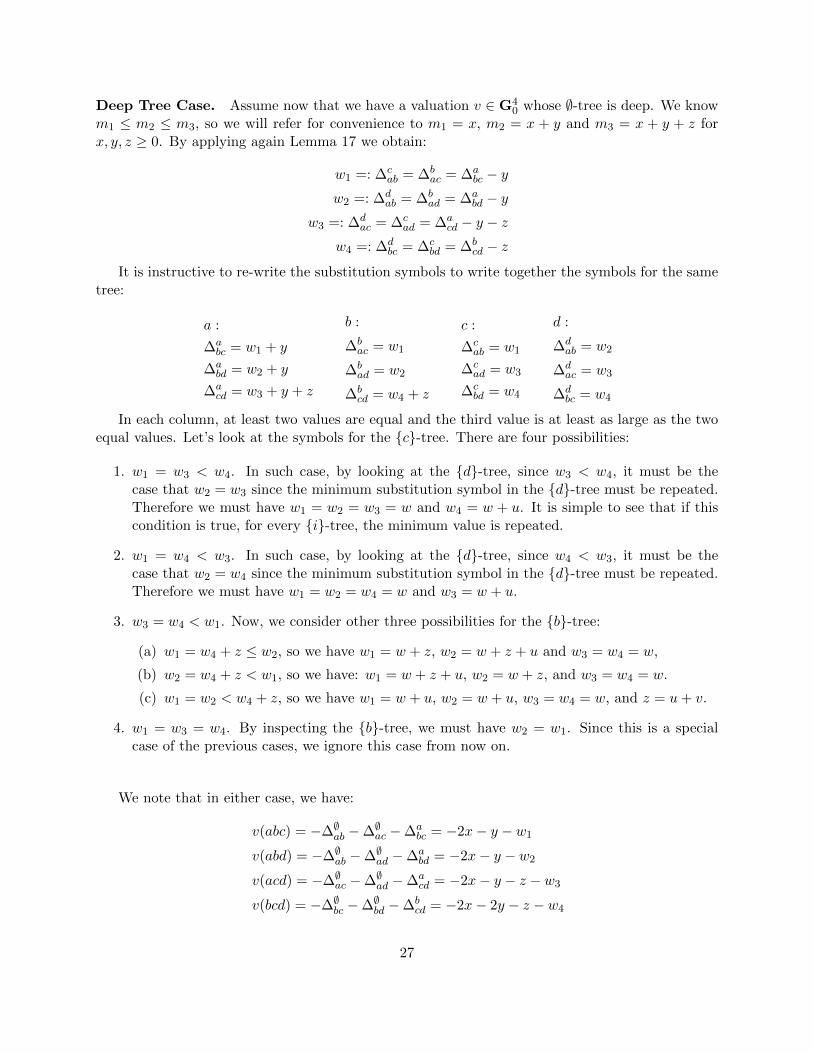
Deep Tree Case. Assume now that we have a valuation v ∈ G40 whose ∅-tree is deep. We know

m1 ≤ m2 ≤ m3, so we will refer for convenience to m1 = x, m2 = x + y and m3 = x + y + z forx, y, z ≥ 0. By applying again Lemma 17 we obtain:

w1 =: ∆cab = ∆b

ac = ∆abc − y

w2 =: ∆dab = ∆b

ad = ∆abd − y

w3 =: ∆dac = ∆c

ad = ∆acd − y − z

w4 =: ∆dbc = ∆c

bd = ∆bcd − z

It is instructive to re-write the substitution symbols to write together the symbols for the sametree:

a :

∆abc = w1 + y

∆abd = w2 + y

∆acd = w3 + y + z

b :

∆bac = w1

∆bad = w2

∆bcd = w4 + z

c :

∆cab = w1

∆cad = w3

∆cbd = w4

d :

∆dab = w2

∆dac = w3

∆dbc = w4

In each column, at least two values are equal and the third value is at least as large as the twoequal values. Let’s look at the symbols for the {c}-tree. There are four possibilities:

1. w1 = w3 < w4. In such case, by looking at the {d}-tree, since w3 < w4, it must be thecase that w2 = w3 since the minimum substitution symbol in the {d}-tree must be repeated.Therefore we must have w1 = w2 = w3 = w and w4 = w + u. It is simple to see that if thiscondition is true, for every {i}-tree, the minimum value is repeated.

2. w1 = w4 < w3. In such case, by looking at the {d}-tree, since w4 < w3, it must be thecase that w2 = w4 since the minimum substitution symbol in the {d}-tree must be repeated.Therefore we must have w1 = w2 = w4 = w and w3 = w + u.

3. w3 = w4 < w1. Now, we consider other three possibilities for the {b}-tree:

(a) w1 = w4 + z ≤ w2, so we have w1 = w + z, w2 = w + z + u and w3 = w4 = w,

(b) w2 = w4 + z < w1, so we have: w1 = w + z + u, w2 = w + z, and w3 = w4 = w.

(c) w1 = w2 < w4 + z, so we have w1 = w + u, w2 = w + u, w3 = w4 = w, and z = u+ v.

4. w1 = w3 = w4. By inspecting the {b}-tree, we must have w2 = w1. Since this is a specialcase of the previous cases, we ignore this case from now on.

We note that in either case, we have:

v(abc) = −∆∅ab −∆∅ac −∆abc = −2x− y − w1

v(abd) = −∆∅ab −∆∅ad −∆abd = −2x− y − w2

v(acd) = −∆∅ac −∆∅ad −∆acd = −2x− y − z − w3

v(bcd) = −∆∅bc −∆∅bd −∆bcd = −2x− 2y − z − w4

27

By Corollary 18, v(abcd) = −∆∅ab −∆∅ac −∆∅ad −∆abc −∆a

bd −∆abcd. By Lemma 17 with S = {c}

and triplet abd, and also with S = {d} and triplet abc, ∆abcd = t+ z+ u for some t ≥ 0. In addition,

we also have ∆∅ab = ∆∅ac = ∆∅ad = x,∆abc = w1 + y, and ∆a

bd = w2 + y. Thus,

v(abcd) = −3x− 2y − w1 − w2 − z − u− t.

Now, following the same procedure used in the previous section, we have that in each case wehave:

• Case 1: v ∈ E4 +∑6

j=1 rj · R+ where r1, . . . , r6 are the ranks of the following matroids:

U14 ,

b

c

d

a ,c

d

ab , U2

4 ,

b c

d

a , U34

• Case 2: Same as before but with the rank functions of the following matroids:

U14 ,

b

c

d

a ,c

d

ab , U2

4 ,

a c

d

b , U34

• Case 3a: Same as before but with the rank functions of the following matroids:

U14 ,

b

c

d

a ,c

da b

, U24 ,

a b

d

c , U34

• Case 3b: Same as before but with the rank functions of the following matroids:

U14 ,

b

c

d

a ,c

da b

, U24 ,

a b

cd , U3

4

• Case 3c: Same as before but with the rank functions of the following matroids:

U14 ,

b

c

d

a ,c

da b

, U24 ,

c

d

ab , U3

4 .

28