On the completeness of hierarchical tensor-product B-splines

Journal of Computational and Applied Mathematics 271 (2014) 53–70

Contents lists available at ScienceDirect

Journal of Computational and AppliedMathematics

journal homepage: www.elsevier.com/locate/cam

On the completeness of hierarchical tensor-product B-splinesDominik Mokriš ∗, Bert Jüttler, Carlotta GiannelliInstitute of Applied Geometry, Johannes Kepler University of Linz, Altenberger Str. 69, 4040 Linz, Austria

a r t i c l e i n f o

Article history:Received 27 November 2013Received in revised form 4 April 2014

MSC:65D07

Keywords:Hierarchical basesTensor-product B-splinesLocal refinementDecoupled hierarchical bases

a b s t r a c t

Given a grid in Rd, consisting of d bi-infinite sequences of hyperplanes (possibly withmultiplicities) orthogonal to the d axes of the coordinate system, we consider the spaces oftensor-product spline functions of a given degree on a multi-cell domain. Such a domainconsists of finite set of cells which are defined by the grid. A piecewise polynomial functionbelongs to the spline space if its polynomial pieces on adjacent cells have a contactaccording to the multiplicity of the hyperplanes in the grid. We prove that the connectedcomponents of the associated set of tensor-product B-splines, whose support intersectsthe multi-cell domain, form a basis of this spline space. More precisely, if the intersectionof the support of a tensor-product B-spline with the multi-cell domain consists of severalconnected components, then each of these components contributes one basis function. Inorder to establish the connection to earlier results, we also present further details relatingto the three-dimensional case with single knots only.

A hierarchical B-spline basis is defined by specifying nested hierarchies of spline spacesand multi-cell domains. We adapt the techniques from Giannelli and Jüttler (2013) to themore general setting and prove the completeness of this basis (in the sense that its spancontains all piecewise polynomial functions on the hierarchical grid with the smoothnessspecified by the grid and the degrees) under certain assumptions on the domain hierarchy.

Finally, we introduce a decoupled version of the hierarchical spline basis that allowsto relax the assumptions on the domain hierarchy. In certain situations, such as quadratictensor-product splines, the decoupled basis provides the completeness property for anychoice of the domain hierarchy.

© 2014 Elsevier B.V. All rights reserved.

1. Introduction

Hierarchical tensor-product splines were introduced by Forsey and Bartels [1] as a tool for adaptive surface modeling.About ten years later, Kraft [2] defined a basis and a quasi-interpolation operator for these spline spaces. At the same time,these splines were used for adaptive surface fitting [3].

Since the advent of isogeometric analysis (IGA), which was established in 2005 as a new approach to bridge the gapbetween analysis and design in engineering applications [4], there is a renewed interest in adaptive and hierarchicaltechniques for tensor-product splines.

The early approaches to adaptive refinement in IGAwere basedmostly on T -splines [5,6]. These originatedmore recentlythan hierarchical B-splines in geometric modeling [7]. It was observed, however, that hierarchical B-splines possess anumber of useful theoretical and practical properties thatmake themwell-suited for numerical simulation based on IGA [8].It has been shown that

∗ Corresponding author. Tel.: +43 0 732 2468 4080.E-mail addresses: [email protected] (D. Mokriš), [email protected] (B. Jüttler), [email protected] (C. Giannelli).

http://dx.doi.org/10.1016/j.cam.2014.04.0010377-0427/© 2014 Elsevier B.V. All rights reserved.

http://dx.doi.org/10.1016/j.cam.2014.04.001

http://www.elsevier.com/locate/cam

http://www.elsevier.com/locate/cam

http://crossmark.crossref.org/dialog/?doi=10.1016/j.cam.2014.04.001&domain=pdf

mailto:[email protected]



http://dx.doi.org/10.1016/j.cam.2014.04.001

54 D. Mokriš et al. / Journal of Computational and Applied Mathematics 271 (2014) 53–70

• these adaptive splines can be equipped with a simple basis that provides the partition of unity and improves the sparsityproperties [9];

• this basis is strongly stable with respect to the L∞ norm [10];• and these functions can be implemented efficiently using standard data structures [11].

There is a growing number of papers on hierarchical methods in IGA [12–14].A new kind of splines has been introduced recently [15], known as LR-splines (LR stands for ‘‘locally refined’’). The use of

this new approach in the application context, as well as its comparison with existing local refinement methods, are still ata preliminary stage.

Simultaneously, adaptive and locally refined spline spaceswere considered from an algebraic viewpoint. The general goalis to determine the dimension of the spline space (which contains all piecewise polynomial functions of a certain degree andsmoothness) and to construct its basis, given a certain partition of the domain into axis-aligned boxes. In the rich literatureon this topic [16–23] several valuable contributions for various cases have been described.

Under certain conditions, the hierarchical spline basis spans the entire space of all piecewise polynomial functions ofthe given degree and smoothness that are defined on the underlying grid (which may possess T -joints) and is thereforecomplete. Such conditionswere first studied in [24] for the bivariate case of uniformdegrees, dyadic refinement andmaximalsmoothness. Based on the algebraic framework (homology techniques) described in [21], a number of recent manuscriptsand preprints presented several generalizations. We mention the recent article [25] that addresses the three-dimensionalcase and the follow-up papers [26,27].

The present paper introduces a different approach. It is based on the observation that the completeness of the hierarchicalspline space can be studied without using advanced results from algebraic homology, but employing solely standardmethods from the theory of tensor-product spline functions. The simple approach presented in this paper allows sufficientconditions to be derived for complete hierarchical spline spaces in any dimension, and for any smoothness (which does nothave to be the same for all grid hyperplanes) and any degree.

The remainder of this paper consists of three main sections and an Appendix. First we analyze dimensions and basesof tensor-product spline spaces on multi-cell domains in Section 2. The Section 3 is devoted to the completeness of thehierarchical B-spline basis in the most general case. Finally, in Section 4 we introduce the decoupled hierarchical basisthat allows to relax – and in some situations even to eliminate – the constraints on the considered domain hierarchy. TheAppendix analyzes the dimensions of tensor-product spline spaces in the trivariate case with single knots.

2. Splines on multi-cell domains

This section derives a basis for tensor-product splines on multi-cell domains. After presenting the necessary definitions,we will prove that this spline space is spanned by a basis consisting of all connected components of the tensor-productB-splines whose support intersects the multi-cell domain. More precisely, if the intersection of the support of a tensor-product B-spline with the multi-cell domain consists of several connected components, then each of them contributes onebasis function.

2.1. Tensor-product B-splines

Given a positive integer d that specifies the dimension of the space, we consider the d-dimensional space Rd withcoordinates x = (x1, . . . , xd). In addition, we consider d bi-infinite strictly increasing sequences of real numbers

gi,jj∈Z , gi,j < gi,j+1,

for i = 1, . . . , d, which will be called the nodes. Using these sequences of nodes we define the grid G to consist of gridhyperplanes

Gi,j = x ∈ Rd| xi = gi,j

with associatedmultiplicities mi,j, which do not need to be the same for all the hyperplanes in the grid.In addition, we choose a degree p = (p1, . . . , pd), where all pi are positive integers. We denote the set of tensor-product

B-splines defined on this grid by B. More precisely, these tensor-product B-splines are products of d univariate B-splineswith the variables xi that are defined by the bi-infinite knot vectors

(. . . , gi,j−1, . . . , gi,j−1 mi,j−1 times

, gi,j, . . . , gi,j mi,j times

, gi,j+1, . . . , gi,j+1 mi,j+1 times

, . . .),

where each knot appears as often as specified by the multiplicity of the associated hyperplane. These tensor-productB-splines are well-defined and continuous if the multiplicities satisfy

1 ≤ mi,j ≤ pi. (2.1)

In the sequel we will denote the tensor-product B-splines β ∈ B simply as B-splines.

D. Mokriš et al. / Journal of Computational and Applied Mathematics 271 (2014) 53–70 55

Fig. 1. The set Bc for biquadratic B-splines with single knots. The small circles correspond to Greville points representing the functions in Bc with respectto the gray cell c.

We consider d indices j1, . . . , jd ∈ Z. The closed set

d

Xi=1

[gi,ji−1, gi,ji ], (2.2)

which is the Cartesian product of d closed intervals between adjacent nodes, is called a cell of the grid. The set of all cellswillbe denoted by C and we use c ∈ C to denote an individual cell.

Consider a cell c ∈ C . We define the set of all B-splines whose support includes this cell,

Bc = β ∈ B | c ⊂ supp β, (2.3)

where the symbol supp denotes the support of a function, i.e.,

supp g = x ∈ Rd| g(x) = 0.

In the case of B-splines, this is an open set, provided that the multiplicity of each knot is at most equal to the degree asassumed in (2.1).

Example 2.1. Fig. 1 shows an example of a set Bc . We consider biquadratic B-splines on a uniform grid with all multiplicitiesequal to 1. The cell c is shown in gray. The support of each basis function consists of 3 × 3 cells; the basis functions thatbelong to the set Bc are represented by the small circles in the centers of their supports, which coincide with their Grevillepoints.

Consider a polynomial f of multi-degree p, i.e., f is a polynomial with the variables xi, where the degree with respect to xiis at most pi. We denote the linear space of all such polynomials by Πp(Rd).

When restricting f and Πp(Rd) to this cell, we obtain the linear space

Πp(c) :=f |c | f ∈ Πp(Rd)

.

The restriction f |c can be expressed as a linear combination of the tensor-product B-splines in Bc ,

f |c(x) =

β∈Bc

λβc (f |c)β|c(x), x ∈ c, (2.4)

where λβc (f |c) is the coefficient of β ∈ Bc in the local representation of the polynomial f on the cell c . Note that f is a

polynomial defined on Rd, whereas f |c is defined on c only.

Example 2.2. Consider again the example of biquadratic splines in Fig. 1. Each cell c ∈ C is influenced by nine basis functionsfrom Bc and each biquadratic polynomial on this cell can be uniquely represented as a linear combination of these ninefunctions.

2.2. Contact of polynomial pieces

We denote the partial derivatives of a polynomial f by

∂ji f :=

∂ jf∂(xi)j

.

Given a polynomial f |c on a cell c , we define its partial derivatives by considering its canonical extension to Rd,

∂ji (f |c) := (∂

ji f )|c,

thereby avoiding the need to consider one-sided limits at the boundary of c.


Consider two cells c, c ′∈ C . There exist indices ji, j′i ∈ Z such that

c =

d

Xi=1

[gi,ji , gi,ji+1] and c ′=

d

Xi=1

[gi,j′i , gi,j′i+1].

The intersection of these cells is an axis-aligned box whose dimension is at most d. If the intersection is non-empty, then itcan be written as

c ∩ c ′=

d

Xi=1

[gi,ai , gi,bi ], (2.5)

where ai = maxji, j′i and bi = minji, j′i + 1. Note that the i–th interval (where i = 1, . . . , d) in the Cartesian productdegenerates to a single point if ji = j′i + 1 or j′i = ji + 1.

Definition 2.3. Consider two polynomials f , f ′ of degree p and two cells c, c ′∈ C , thus f |c ∈ Πp(c) and f ′

|c′ ∈ Πp(c ′). Wesay that the polynomial f |c on the cell c and the polynomial f ′

|c′ on the cell c ′ have a contact on c ∩ c ′ (and write f |c ∼ f ′|c′ )

if

∀x ∈ c ∩ c ′: (∂

j11 · · · ∂

jdd f |c)(x) = (∂

j11 · · · ∂

jdd f ′

|c′)(x) (2.6)

is satisfied for all

ji = 0, . . . , pi − minmi,ai ,mi,bi, i = 1, . . . , d, (2.7)

where c ∩ c ′ has the form (2.5) (or is empty) and mi,ai and mi,bi are the multiplicities of the grid hyperplanes Gi,ai and Gi,bi ,respectively.

In particular, any two polynomials on disjoint cells have a contact, since c ∩ c ′ is empty in this case. The relation ∼, whichacts on pairs of polynomials and cells, is symmetric and reflexive, but not transitive.

The order of the contact depends on the givenmultiplicity of the grid hyperplanes: the higher themultiplicity, the smallerthe number of derivatives that have to agree.

Note that if ai < bi holds for some coordinate direction i in the representation (2.5) of the (nonempty) intersection c ∩ c ′

(namely, when ji = j′i), then the Eq. (2.6) is even satisfied for all positive integers ji, since we can differentiate the equationsobtained for the ranges of indices ji specified in (2.7) with respect to xi.

From now on we will use the notation

β|c∩c′ = 0

to express the fact that the B-spline β does not vanish identically on c ∩ c ′, i.e.,

∃x ∈ c ∩ c ′: β(x) = 0.

The contact between two polynomials on different cells can be characterized easily with the help of the B-splinecoefficients.

Lemma 2.4 (Contact Characterization Lemma—CCL). The two polynomials f |c and f ′|c′ that were considered in Defini-

tion 2.3 have a contact on c ∩ c ′ if and only if

∀β : β|c∩c′ = 0 ⇒ λβc (f |c) = λ

β

c′(f′|c′). (2.8)

Proof. This can be proved by extending the univariate blossoming argument to the tensor-product setting (see, e.g., [28,Section 7.1]; the extension would proceed analogously to the similar generalization for multivariate Bézier surfaces, whichis outlined in [28, Section 9.7]). Indeed, the two polynomials have a contact if and only if the associated values of theirblossoms (which then correspond to the B-spline coefficients) agree.

Alternatively, one may prove this observation with the help of the tensor-product Bernstein–Bézier (BB) representationof the two polynomials with respect to the associated cells. The values and derivatives that characterize the contact areuniquely determined by the two subsets of the BB coefficients (determining sets) of both polynomials. The polynomialshave a contact if and only if the coefficients of the determining set of f |c can be generated by applying a certain bijectivelinear mapping to the coefficients of the determining set of f ′

|c′ . On the other hand, the subset of the B-spline coefficientsconsidered in (2.8) is linked to each of the coefficients of the twodetermining sets by twoother bijective linearmappings thatcan be found via knot insertion. Due to the bijectivity of all mappings, choosing the same B-spline coefficients considered in(2.8) for both polynomials is the only possibility to obtain a contact.

In order to keep this paper concise, we do not present the technical details of either proof.


(a)

(b) (c) (d)

Fig. 2. (a) The 16 bicubic B-splines in Bc related to the case of double horizontal and single vertical knots; (b)–(d) three possibilities of a contact. TheB-splines whose supports intersect the first and second cell are depicted by solid symbols ( , ) and by squares (, ), respectively. The support of anyB-spline represented by a solid square () intersects both cells.

Example 2.5. We consider the bivariate case with double horizontal knots and single vertical knots in Fig. 2. There aresixteen bicubic B-splines whose supports intersect each cell (a). Considering two cells that are different from each other,there are four possibilities of a contact between polynomials.• The cells are disjoint and all polynomials have a contact (not shown).• The cell share a vertical edge (b). All values and derivatives of order 0 or 1with respect to x1 and of any order with respect

to x2 have the same value on the vertical edge.• The cells share a horizontal edge (c). All values and derivatives of any order with respect to x1 and of order 0, 1, or 2 with

respect to x2 have the same value on the horizontal edge.• The cells share a grid point (d). All values and derivatives of order 0 and 1 with respect to x1 and of order 0, 1, or 2 with

respect to x2 have the same value at the grid point.

2.3. Piecewise polynomials on multi-cell domains

We consider a finite subset M ⊂ C which we will call a multi-cell domain. More precisely, the set M contains a finitenumber of cells of the form (2.2). Furthermore, we will use the abbreviation

M =

M =

c∈M

c

for the subset of Rd occupied by the cells from M . The set M is a closed and bounded subset of Rd. To simplify the notationit will be often also called multi-cell domain, whenever confusion is improbable.

Definition 2.6. Given a multi-cell domain M ⊂ C we define the disconnected space (also called the space of piecewisepolynomials) by

P(M) = s = (sc)c∈M | sc ∈ Πp(c).

Thus any piecewise polynomial s ∈ P(M) is a collection of polynomials sc , one for each cell c ∈ M . Each of thesepolynomials sc is actually the restriction of a globally defined polynomial sc ∈ Πp(Rd) to the corresponding cell, i.e.,sc = sc |c—see the end of Section 2.1. However, we will not need to refer to the globally defined polynomials sc throughoutthe paper.

Note that these polynomials may take different values at the grid lines. Therefore, it is generally impossible to define acontinuous function s on M such that s|c = sc for all c ∈ M .

Nevertheless, each sc can be represented in the B-spline basis as observed in (2.4):

sc(x) =

β∈Bc

λβc (sc)β|c(x), x ∈ c, c ∈ M.


Definition 2.7. We consider a multi-cell domain M and the associated disconnected space P(M). The spline space on M isdefined by

S(M) = s ∈ P(M) | ∀c, c ′∈ M : sc ∼ sc′. (2.9)

For s ∈ S(M) we define s : M → R so that

s(x) = sc(x), if x ∈ c and c ∈ M.

This function is well-defined (single-valued), since any two polynomial pieces sc and sc′ meet at least continuously alongthe intersection c ∩ c ′ of any two neighboring cells. By using the characteristic functions χc of the cells c ∈ M , we mayexpress it in terms of the basis functions as follows:

s(x) =

c∈M

β∈Bc

λβc (sc)β(x)χ ⋆

c (x), x ∈ M, (2.10)

with the normalized characteristic functions

χ ⋆c (x) =

χc(x)

k∈Mχk(x)

, if x ∈ M,

0, otherwise.

Note that the characteristic functions need to be normalized in order to obtain the correct values also on grid hyperplanes.Strictly speaking, the elements of S(M) are |M|-tuples of polynomials, where |M| is the number of cells inM . In order to

keep the notation simple, we will use the same notation for the actual spline functions s.That is, we will consider the elements of S(M) simultaneously as |M|-tuples of polynomials and as piecewise polynomial

functions defined onM. Consequently, wewill simply write s instead of s, and wewill denote the linear space of all piecewisepolynomial functions on M with the required contacts between the polynomial segments as S(M).

Definition 2.8. Consider a basis function β ∈ B. Its coefficient graph Γβ is defined as follows.

• The vertices of Γβ are the cells c ∈ M such that c ⊂ supp β .• Two vertices c and c ′ are connected by an edge iff β|c∩c′ = 0.

The set of connected components of this graph will be denoted by K(Γβ).

If there is no overlap of β with M then both the coefficient graph Γβ and the set K(Γβ) of connected components areempty.

We use the notation

c ε Γβ

to express the fact that the cell c is a vertex of the coefficient graph Γβ . Similarly, when considering a connected componentΦ ∈ K(Γβ) – which is a subgraph of Γβ – all cells c satisfying c ε Φ are exactly the vertices of Φ .

Example 2.9. We consider again the biquadratic case. Fig. 3 shows a multi-cell domain consisting of nine cells (a), thesupports of three basis functions β1, β2 and β3 (b), together with their coefficient graphs (c). The coefficient graphs of β2and β3 have only one connected component, while the coefficient graph of β1 possesses two of them.

Proposition 2.10. Consider a piecewise polynomial s ∈ P(M). It is contained in the spline space S(M) if and only if the coefficientssatisfy λ

βc (sc) = λ

β

c′(sc′) for all basis functions β ∈ B and for all c and c ′ belonging to the same connected component of Γβ .

Proof. Consider a piecewise polynomial s ∈ S(M) and a basis functionβ ∈ B. Assume there exist c, c ′ in the same connectedcomponent such that λβ

c (sc) = λβ

c′(sc′). Then there exist two vertices k and k′, k∩ k′= ∅, in this connected component such

that λβ

k (sk) = λβ

k′(sk′). According to CCL (Lemma 2.4), sk and sk′ do not have a contact and therefore s does not belong toS(M).

On the other hand, if all coefficients λβc (sc) associated to any β ∈ B for all cells c belonging to one connected component

of Γβ take the same value, then all sc have a contact by CCL (Lemma 2.4). Since the cells in these connected componentscoverM , we may conclude that s ∈ S(M).

2.4. Spline bases on multi-cell domains

Definition 2.11. For every β ∈ B and every connected component Φ ∈ K(Γβ) we define the function

βΦ(x) =

c ε Φ

β(x)χ ⋆c (x).


(a) Multi-cell domain. (b) Three examples of B-splines βi .

(c) Coefficient graphs associated with βi, i = 1, 2, 3.

Fig. 3. A multi-cell domain with nine cells (a), the supports of three biquadratic B-splines (b) and the associated coefficient graphs (c).

The set of all these functions is denoted by

∆ =

β∈B

βΦ | Φ ∈ K(Γβ).

Theorem 2.12. The set ∆ – when restricted to M – forms a locally linearly independent basis of S(M).

Proof. Consider s ∈ S(M). First,we prove that s can be obtained as a linear combination of functions from∆. Since, accordingto Definition 2.8, the vertices of Γβ are the cells c ∈ M that are contained in the support of β , Eq. (2.10) can be rewritten asfollows:

s(x) =

β∈B

c ε Γβ


c (x) =

β∈B

Φ∈K(Γβ )

c ε Φ


c (x), (2.11)

where x ∈ Rd. In virtue of Proposition 2.10, for each β ∈ B and for each Φ ∈ K(Γβ), all the coefficients λβc (sc) have to be

the same for all c ε Φ . We will denote this coefficient by ΛβΦ(s). Thus, we may rewrite (2.11) as

s(x) =

β∈B

Φ∈K(Γβ )

ΛβΦ(s)

c ε Φ

β(x)χ ⋆c (x)

=βΦ∈∆

.

Second, we prove the local linear independence of the functions. Consider an open subset X ⊂ M and a linear combina-tion of functions βΦ ∈ ∆ that do not vanish on X , which is equal to zero on X . For each βΦ we consider a cell c ε Φ , that hasa nonempty intersection with X . Clearly, βΦ does not vanish on c. Moreover, the restrictions of all functions βΦ to this cellare either zero or equal to the restrictions of mutually different tensor-product B-splines β ∈ B. From the local linear inde-pendence of functions β ∈ Bwe then obtain that the coefficient of βΦ in the linear combination is zero. Repeating this for allfunctions βΦ , we conclude that the functions βΦ are locally linearly independent. This also implies the linear independenceof ∆.

Corollary 2.13. If for each β the intersection of its support with the multi-cell domain M is connected, then the functions in

BM = β ∈ B | supp β ∩ M = ∅,

when restricted to M, form a basis of S(M).

Proof. Indeed, if this condition is satisfied, then each coefficient graph in Theorem2.12 has either one connected componentor it is empty.


Fig. 4. The support of a bicubic B-spline that violates the assumption of Corollary 2.13 with respect to the domain consisting of all the gray cells.

Example 2.14. The condition concerning the connected sets in Corollary 2.13 means that there is no situation like the oneshown in Fig. 4 for bicubic B-splines on a grid with single knots.

Appendix analyzes the case of trivariate spline spaces with single knots, which has been discussed in [25]. We show thattheir result (which, however, is limited to a special class of multi-cell domains) is a special case of Corollary 2.13.

3. Hierarchical splines

We now use the notation introduced in the previous section in a hierarchical setting to define a hierarchical spline spaceand a certain hierarchical basis. Subsequently, we prove that this hierarchical basis spans the entire hierarchical spline space.

3.1. Hierarchies of tensor-product spline spaces

In order to define a hierarchical tensor-product spline space, we need to introduce a hierarchy of tensor-product splinespaces and a hierarchy of domains.

First, we consider the spline spaces. Given a maximal level N , we consider a sequence of grids Gℓ, ℓ = 0, . . . ,N , withassociated degrees pℓ

= (pℓ1, . . . , p

ℓd) where we assume that the degrees do not decrease,

pℓ≤ pℓ+1, that is pℓ

i ≤ pℓ+1i , i = 0, . . . , d, ℓ = 0, . . . ,N − 1.

Each grid hyperplane Gℓi,j ∈ Gℓ has an associated multiplicitymℓ

i,j that satisfies the assumption (2.1) level by level.We assume that the grids are nested in the following sense: every grid hyperplane in Gℓ is also present in Gℓ+1 and

its multiplicity in the higher level is at least equal to the previous multiplicity plus the increase of the degree in thecorresponding coordinate direction.

Based on the sequence of grids and degrees, we now define on each grid Gℓ the set of tensor-product B-splines Bℓ ofdegree pℓ. The spans of the B-splines define the spline spaces

Vℓ= span Bℓ, ℓ = 0, . . . ,N.

Under the previous assumptions concerning non-decreasing degrees and nested grids, the linear spaces spanned by theB-splines are nested, i.e.,

Vℓ⊆ Vℓ+1, ℓ = 0, . . . ,N − 1.

For each level ℓ, the grid Gℓ and the degrees pℓ allow to apply the theory from Section 2. Thus, if we are given a multi-cell domain Mℓ with respect to the grid Gℓ, we may define a spline space Sℓ(Mℓ). Note that the restriction of Vℓ to Mℓ iscontained in this spline space,

Vℓ|Mℓ ⊆ Sℓ(Mℓ).

The connected components of the B-splines from Bℓ with respect to the multi-cell domain

Mℓ=

c∈Mℓ

c

form a basis of this space according to Theorem 2.12.In addition, we consider a nested sequence of domains

Ω0⊇ Ω1

⊇ · · · ⊇ ΩN= ∅, (3.1)

which will be called the domain hierarchy. We assume that these domains satisfy the following.


Fig. 5. Hierarchical mesh consisting of cells from three levels.

(a) Ω0 . (b) Ω1 . (c) Ω2 .

Fig. 6. DomainsΩ0, Ω1 andΩ2 associated with themesh in Fig. 5. Grid lines from level 0, 1, 2 are depicted as solid, dashed, and dotted lines, respectively.

(a) M0 . (b) M1 . (c) M2 .

Fig. 7. Rings associated with the mesh in Fig. 5.

Assumption 3.1. Each set

Ω0\ Ωℓ+1, ℓ = 0, . . . ,N − 1,

can be represented as amulti-cell domainwith respect to the gridGℓ. More precisely,we assume that there exists amulti-celldomainMℓ

⊆ Cℓ, which is a finite set of cells of the grid Gℓ, satisfying

Ω0\ Ωℓ+1

= Mℓ.

For convenience, we define

M−1= ∅.

The sets

Mℓ= Ω0

\ Ωℓ+1

were denoted as rings in [24], because, conceptually, they represent the domainΩ0 with the ‘‘hole’’Ωℓ+1. Wewill also adoptthis concept. However, the above assumption concerning the shape of the rings is actuallyweaker than the one in [24],whereeach Ωℓ was assumed to be a multi-cell domain of level max(0, ℓ − 1).

Note that these rings are also nested,

Ω0= MN−1

⊇ MN−2⊇ · · · ⊇ M0

⊇ M−1= ∅.

Example 3.2. Fig. 5 shows a hierarchical mesh. The corresponding domains are shown in Fig. 6 and the associated rings aredepicted in Fig. 7. As already mentioned, Assumption 3.1 does not require the boundary of each Ωℓ to be aligned with theknots lines associated to the previous level ℓ − 1, as it was assumed in [24]. For instance, the small L-shaped subdomain atlevel 2 on the bottom right corner of the mesh was disallowed in [24].

Based on the sequences of function spaces and domains, we are now able to define the hierarchical spline space, providedthat the restriction of a function to each of the multi-cell domains Mℓ belongs to the corresponding spline space Sℓ(Mℓ):


Definition 3.3. The hierarchical spline space H is given by

H = h : Ω0→ R | ∀ℓ : h|Mℓ ∈ Sℓ(Mℓ).

According to this definition, a function is contained in the hierarchical space if it is a piecewise polynomial function onthe hierarchical grid defined by the nested grids and domains, where the individual polynomial segments meet with thesmoothness specified by the degrees and the multiplicities of the grid hyperplanes. Note that this is more general than justrequiring that

h|Mℓ ∈ Vℓ|Mℓ .

3.2. The basis of the hierarchical spline space

Recall that we have defined a tensor-product spline basis Bℓ on each grid Gℓ. Similarly to (2.3) we consider the B-splineswhose support intersects the ring Mℓ:

Bℓ

Mℓ := β ∈ Bℓ| supp β ∩ Mℓ

= ∅.

Based on the definition of the rings, we again use the selection procedure from [24], which slightly generalizes the earliermethod proposed by Kraft in [2] by also allowing for coinciding subdomain boundaries.

Definition 3.4. The hierarchical basis K is defined as

K =

N−1ℓ=0

Kℓ

with

Kℓ= β ∈ Bℓ

Mℓ | supp β ∩ Mℓ−1= ∅.

Thanks to the local linear independence of the bases Kℓ⊂ Bℓ, it can be shown that the set K of hierarchical B-splines is

linearly independent, see [2] or [8].Now we are able to formulate the main result of this paper.

Theorem 3.5. If the assumption of Corollary 2.13 is satisfied for each level ℓ, i.e., if for any ℓ = 0, . . . ,N − 1, and any β ∈ Bℓ

the set supp β ∩ Mℓ is connected, then the hierarchical spline basis K from Definition 3.4 spans the entire space H.

Proof. The proof is rather similar to the proof of Theorem20 in [24]. Nevertheless, in order tomake this paper self-contained,we repeat it here in a shorter form.

We consider a function h ∈ H. The proof consists of two steps. First, we show that there exist N functions hℓ∈

span Bℓ

Mℓ , ℓ = 0, . . . ,N − 1, such that

hℓ|Mℓ =

h −

ℓ−1i=0

hi

Mℓ

. (3.2)

This can be proved by inductionwith respect to ℓ. In each step, the right hand side of (3.2) can be shown to belong to Sℓ(Mℓ),hence Corollary 2.13 implies the existence of hℓ.

Second, it can be shown by analyzing the right-hand side of Eq. (3.2) that hℓ|Mℓ−1 = 0. Therefore, the local linear

independence of the B-splines implies that hℓ∈ span Kℓ.

Finally, by rewriting (3.2) for ℓ = N − 1, we obtain

h|MN−1 =

N−1i=0

hi|MN−1 ,

which concludes the proof, since MN−1= Ω0, hi

∈ span K i, andN−1

i=0 K i= K .

The assumptions of Theorem 3.5 are satisfied if each subdomain Ωℓ is either sufficiently small or sufficiently large withrespect to the supports of the B-splines at the previous level. This condition is slightly weaker than the assumptions ofTheorem 20 in [24].

Example 3.6. Consider the case where all the degrees (at all levels and in all coordinate directions) are equal to p and all themultiplicities of hyperplanes are equal to 1. In this case, when considering dyadic refinement only, a sufficient condition forthe assumptions of Theorem 3.5 to be satisfied is that there is a finite set I such that

Ωℓ=

i∈I

Ωℓi , where

Ωℓ

i

∩Ωℓ

j

= ∅ for i, j ∈ I, i = j


Fig. 8. A domain Ωℓ= Ωℓ

0 ∩ Ωℓ1 that satisfies the assumptions of Theorem 3.5 for p = 3 as specified in Example 3.6. We show the interior of Ω0

\ Ωℓ

(dark gray cells), Ωℓ0 and Ωℓ

1 (light gray cells), the offset of Ω0\ Ωℓ

0 at distance 1 (thick black line) and a box of 2 × 2 cells containing Ωℓ1 (hatched light

gray cells). The dashed lines represent the grid Gℓ−1 .

(that is, the interiors of the sets Ωℓi are mutually disjoint) and each Ωℓ

i is such that either

• Ω0\ Ωℓ

i admits an offset1 at distance (p − 1)/2 with respect to the grid Gℓ−1 or• Ωℓ

i is contained in a box consisting of (p − 1) × · · · × (p − 1) cells of the grid Gℓ−1.

Fig. 8 provides a bivariate example.

4. The decoupled hierarchical basis

We introduce a decoupling mechanism, which is inspired by the so-called truncation introduced in [9]. It can be suitablyexploited in order to relax the assumptions of Theorem 3.5.

We consider the representation of a B-spline β with respect to the next (i.e., finer) level in the spline hierarchy. For eachconnected component of β we define a decoupled basis function. This function collects the contributions of those functionsof the next level whose supports have an overlap with a particular connected component of the support of the originalB-spline β , restricted to the associated multi-cell domain Mℓ.

More precisely, we consider the representation of a B-spline β ∈ Bℓ with respect to the basis Bℓ+1 at the next level givenby

β =

γ∈Bℓ+1

cℓ+1γ (β)γ ,

with certain coefficients cℓ+1γ (β) ∈ R, which are determined by the knot insertion algorithm. The function β possesses an

associated coefficient graph Γ ℓβ with respect to the multi-cell domain Mℓ, see Definition 2.8. We consider the connected

components K(Γ ℓβ ) of the coefficient graph and use each of them to define a decoupled function.

Definition 4.1. For each connected component Φ ∈ K(Γ ℓβ ) we define a decoupled basis function

δΦ(β) =

γ∈Bℓ+1: supp γ∩(

Φ)=∅

cℓ+1γ (β)γ , Φ ∈ K(Γ ℓ

β ),

where

Φ =

c ε Φ c denotes the union of the cells that are vertices ofΦ . If the support of each function γ ∈ Bℓ+1 intersectsatmost one of the sets

Φ , then so do the functions δΦ(β). We say that the decoupling is feasible if this condition is satisfied

for all β ∈ Bℓ and for all levels ℓ.

If the decoupling is feasible, then the restriction of the decoupled basis function δΦ(β) to the multi-cell domain Mℓ isidentical to the functionβΦ thatwas defined in Definition 2.11. Consequently, the decoupled functions inherit the propertiesof these functions. In particular, Theorem 2.12 implies the following result.

1 The offset to a domain and its admissibility have been defined in [24] for the case d = 2 and they are defined in the Appendix for d = 3. The latterdefinition extends to any dimension d.


Corollary 4.2. If the decoupling is feasible, then the functions from the set

Dℓ

Mℓ := δΦ(β) | Φ ∈ K(Γ ℓβ ), β ∈ Bℓ

Mℓ, (4.1)

when restricted to Mℓ, form a locally linearly independent basis of Sℓ(Mℓ).Generally, the feasibility of the decoupling depends on the choice of the domains Ωℓ, ℓ = 0, . . . ,N . For certain classes

of spline spaces Vℓ, ℓ = 0, . . . ,N − 1, however, the decoupling is always feasible. We introduce the following definition.

Definition 4.3. A sequence of nested spline spaces (Vℓ)N−1ℓ=0 is said to possess the unconstrained completeness property (UCP)

if the decoupling is feasible at all levels and for any choice of the domains Ωℓ.UCP is automatically granted if the support of each function of level ℓ + 1 is contained in 2 × 2 × · · · × 2 cells of the

grid of level ℓ. Indeed, if this condition is satisfied, then for any choice of the multi-cell domain Mℓ, the intersection of thesupport of a finer function with this multi-cell domain is connected. Special instances of this situation will be presented inExamples 4.5 and 4.6 below.

Corollary 4.4. The functions contained in

D =

N−1ℓ=0

δΦ(β) ∈ Dℓ

Mℓ | supp δΦ(β) ∩ Mℓ−1= ∅ (4.2)

form a basis of the space H, which was introduced in Definition 3.3, provided that the decoupling is feasible at all levels. Inparticular, if the sequence of nested spline spaces has the unconstrained completeness property, then this is true for any choice ofthe domain hierarchy (3.1).Proof. The result can be derived by generalizing the proof of Theorem 3.5. This can be done by simply replacing Bℓ

Mℓ by Dℓ

Mℓ

throughout the original proof.

UCP should be quite useful when designing refinement algorithms that maintain the completeness property. Typically,the refinement is guided by an error estimator that selects the cells that need to be refined. Without UCP, further cells haveto be added in order tomaintain the completeness of the hierarchical space. This is no longer neededwhen using hierarchieswith UCP and the decoupled hierarchical basis D of the spline space.

A sufficient condition for UCP is the following. For any choice of Ωℓ+1 and for any basis function β ∈ Bℓ the support ofany basis function γ ∈ Bℓ+1 with supp γ ⊆ supp β intersects Mℓ in a connected set. Finally, we present two examples ofhierarchies with UCP.

Example 4.5. UCP is satisfied when considering only single knots at all levels and using a refinement strategy that splitsevery cell of level ℓ in pℓ

1 × · · · × pℓd cells of level ℓ + 1.

Example 4.6. When considering dyadic refinement, where every cell of level ℓ is split into 2d cells of level ℓ + 1, UCP issatisfied if the multiplicities are chosen such that the inequalities

3mℓi,j ≥ pℓ

i + 1

hold for all levels, for i = 1, . . . , d and for j ∈ Z.Both examples include quadratic tensor-product splines with dyadic refinement. Special cases of both examples are

shown in Fig. 9. The B-splines β are decoupled into two basis functions δΦ(β) and δΨ (β) associated to the connectedcomponents Φ, Ψ ∈ CC(Γβ). The finer subdomain is the region covered by the finer grid, whereas the coarser subdomaincontains the entire mesh.

5. Closure

We analyzed dimensions and bases of multivariate tensor-product spline functions on a multi-cell domain. Based onthese results, by a slight generalization of the techniques from [24], we derived a simple sufficient condition for the com-pleteness of a hierarchical spline space. More precisely, this condition guarantees that any piecewise polynomial functionson the given hierarchical grid can be represented in the hierarchical tensor-product B-spline basis. In addition, we proposedthe new concept of the decoupled hierarchical basis that allows to relax – and in the case of hierarchies with UCP even toeliminate – the conditions on the domain hierarchy that are required to guarantee the completeness.

Future work will focus on formulas for the dimensions of hierarchical spline spaces, which are currently only givenimplicitly by the number of active tensor-product B-splines, and on applications of multivariate hierarchical B-splines, inparticular in isogeometric analysis.

Acknowledgments

The authors have been supported by the Austrian Science Fund (FWF), NFN S117 ‘‘Geometry + Simulation’’ and by theEC, project EXAMPLE, GA No. 324340. This support is gratefully acknowledged.


Fig. 9. Two bivariate spline hierarchieswith UCP. Top left: bicubic splineswith single knots and triadic refinement. Top right: biquintic splineswith doubleknots and dyadic refinement. Both pictures show the support of a B-spline β (solid black line) and of two decoupled basis functions δΦ (β) and δΨ (β) (redand blue regions) that are derived from the connected components Φ, Ψ of the coefficient graph of β . Bottom: the associated coefficient graphs. (Forinterpretation of the references to colour in this figure legend, the reader is referred to the web version of this article.)

Appendix. The trivariate case with uniform knots and maximal smoothness

Weconsider Corollary 2.13 for spline spaces onmulti-cell domains in three-dimensional spacewithmaximal smoothness(i.e., all the multiplicities are equal to one). For simplicity, we consider uniform knots only, but all results remain valid in thenon-uniform case. We derive formulas that give the number of B-splines, provided that the intersections of their supportswith the multi-cell domains are connected. We show that the results by Berdinsky et al. [25] are a special case of this moregeneral analysis.

Multi-cell domains and their properties have been studied in digital geometry [29]. However, most of the existing resultsare limited to simple polyhedra, i.e., multi-cell domains without kissing vertices and edge segments (see Appendix A.3below), since these polyhedra are preferred in the relevant applications.

A.1. Dilations, offsets, and types of edges and vertices

Each of the basis functions of tri-degree p = (p, p, p), where p is a positive integer, can be identified with• the centroid of the central cell of its support if p is even,• the intersection of eight cells in the middle of the support if p is odd.

In order to derive the number of basis functions that have a support with a non-empty intersection with M, we define thenotion of dilation of a multi-cell domain. Moreover, we consider the so-called combinatorial volume, which is related to thenumber of cells and grid points of a multi-cell domain. The combinatorial volume of a multi-cell domain is then equal to thenumber of the basis functions of the spline space. Recall that the notion of a multi-cell domain refers both to a setM of cellsand to the subset M of R3 that is occupied by them.

Definition A.1. The dilation M(q) of a multi-cell domain M, defined for any even value of q, is recursively obtained as

M(q):=

M, if q = 0,M(q−2)

∪ N(M(q−2)), for q ≥ 2,

whereN(M(q−2)) is the offset region of thickness 1 toM(q−2), i.e., the set of all the cells c ∈ C that are contained inR3 \ M(q−2)

and that share a vertex, an edge or a face with M(q−2).

Clearly, the dilations of a multi-cell domain are again multi-cell domains. A related notion is the following.

Definition A.2. The offset of the multi-cell domain M at distance q/2 is the set

F (q)(M) :=

x ∈ Rd

| infr∈M

maxi=1,...,d

(|ri − xi|) =q2

, (A.1)

where r = (r1, . . . , rd) is a point that belongs to the multi-cell domain M. We assume d = 3.


(a) Domain. (b) Offset surface.

Fig. 10. (a) Example of a multi-cell domain that is admissible for q = 1 but not for q = 2. (b) The non-admissible offset surface at distance 2.

Table A.1The types of boundary edges of a multi-cell domain.

Convex edge (cvx) Non-convex edge (ncx) Kissing edge (ksg)

The right-hand side of (A.1) is the set of points in Hausdorff distance q/2 (with respect to maximum metric) from M.Geometrically, it is a generalization of the notion of the offset curve as defined in [24] to create a surface in three dimensions.

Note that the offset is defined for any nonnegative value of q, while the dilation is defined for even values only.Dilations and offsets are closely related. For even values of q, the boundary of the dilation M(q) is a subset of the offset

F (q)(M). This characterization can be extended to odd values of q also, but we do not need it in this paper.

Definition A.3. The offset F (q)(M) is said to be admissible, or, equivalently,M is said to admit an offset at distance q2 , if either

• q = 0 holds or if• F (q−1)(M) is admissible and all connected components of F (q)(M) are homeomorphic to a closed surface in R3 (i.e., to an

embedded 2-manifold in 3-space).

Example A.4. The multi-cell domain shown in Fig. 10 admits an offset at distance 12 but not at distance 2

2 = 1. Indeed,F (2)(M) is not homeomorphic to a closed surface.

Finally, we introduce another notion, which will be used to count the basis functions that are not identically zero on amulti-cell domain.

Definition A.5. The q-th combinatorial volume of a multi-cell domain M is defined as

ω(q)(M) :=

number of cells of M(q), if q is even;

number of grid points of M(q−1), if q is odd.

By grid pointswe mean the intersections of three grid hyperplanes.

A multi-cell domain can be characterized by various quantities. Its boundary consists of planar patches that consist ofseveral faces (each belonging to only one cell). These patchesmeet in edges that consist of edge segments (each being incidentto two or four faces). The edges meet in vertices. We consider

• the number of cells z,• the number of boundary faces f ,• the number of convex edge segments ecvx, of non-convex edge segments encx and of kissing edge segments eksg (see

Table A.1) on the boundary,• the number of vertices of type i, where i = 1, . . . , 21 according to Table A.2, that will be denoted by vi.

In addition, we use upper indices to denote the number of these quantities for the dilation M(q). For instance, z(q), e(q)cvx

and v(q)i denote the number of cells, convex edge segments, and vertices of type i of the dilation M(q). Clearly, z = z(0) etc.


Table A.2The types of vertices of a multi-cell domain, up to rotations and symmetries and ordered by the number of incident cells. The configurations marked by ⋆ , and + do not correspond to vertices, since they are located within edges, within patches and in the interior of the multi-cell domain, respectively.

1 2⋆ 3 4 5 6 7

8 9 10 11 12⋆ 13 14

15 16 17⋆ 18 19 20 21+

Finally, we introduce the vertex term

v(q)= (v

(q)1 − 2v(q)

3 − 6v(q)4 − 3v(q)

5 − v(q)6 − v

(q)7

− 2v(q)9 − 2v(q)

10 + 4v(q)13 − v

(q)14 + v

(q)15 + 3v(q)

16 + 2v(q)18 + 2v(q)

19 + v(q)20 ) (A.2)

and the edge term

e(q)= e(q)

cvx − e(q)ncx − 2e(q)

ksg. (A.3)

Again, we shall omit the index (q) for q = 0, i.e., we write v = v(0), e = e(0) and f = f (0). Note that if eK = v4 = v19 = 0(see Appendix A.3) then v(q) is equal to T from Theorem 8.6 in [29].

A.2. The dimension of the spline space

We derive the number of B-splines whose support intersects a given multi-cell domain and we specify it in terms ofthe quantities that characterize the domain M. Lemma A.6 gives the formula for these quantities for the dilated domainsM(q) including the combinatorial volumeω(q)(M)when q is even, while Lemma A.7 allows us to compute the combinatorialvolume when q is odd. The dimension of the spline space is then described in Theorem A.8.

Lemma A.6. If the multi-cell domainM admits an offset at distance q/2, where q is even, then the vertex term v(q), the edge terme(q), the number of faces f (q) and the number of cells z(q) of the dilated multi-cell domain M(q) satisfy

v(q)= v, e(q)

= e +3q2

v, f (q)= f + qe +

3q2

4v, z(q)

= z +q2f +

q2

4e +

q3

8v. (A.4)

Moreover, the formula for z(q) is valid even if M admits an offset at distance q−12 only.

Proof. Formulas (A.4) can be verified by induction (with respect to even values of q) using Table A.3. Given the dilationM(q) of a multi-cell domain M, the table specifies how the number of each kind of feature (i.e., faces, edge segments of thethree types, and vertices of the 21 types) of the dilation M(q+2) depends on the numbers of miscellaneous features in M(q),provided that the offset at distance (q+2)/2 is admissible (except for the case of cells where we need only offset at distance(q + 1)/2 to be admissible). This table can be derived by a careful case-by-case analysis.

Lemma A.7. The number of grid points g(M) of a multi-cell domain M is equal to

g(M) = z +f2

+e4

+v

8.

Lemma A.7 can be proved by inspecting various cases similarly to Lemma A.6.


Table A.3Numbers of cells, faces, convex/non-convex/kissing edge segments and vertices of the various types of the dilation M(q+2) that are contributed by eachcell, face, edge segment and vertex of M(q) . The proof of Lemma A.6 is based on this information.

Dilation M(q+2)

Cell Face Edge Vertexcvx ncx ksg 1 3 4 5 6 7 9 10 11 13 14 15 16 18 19 20

Multi-celldomain M(q)

Cell 1Face 1 1

Edgecvx 2 2 1ncx −2 −2 1ksg −4 −4 2

Vertex

1 1 3 3 13 −2 −6 −4 2 24 −6 −18 −6 12 65 −3 −9 −3 6 36 −1 −3 −2 1 17 −1 −3 −3 1 19 −2 −6 −3 3 110 −2 −6 −2 4 211 −1 −1 1 113 4 12 −12 414 −1 −3 −1 2 115 1 3 −3 116 3 9 −9 318 2 6 −6 219 2 6 −6 220 1 3 −3 1

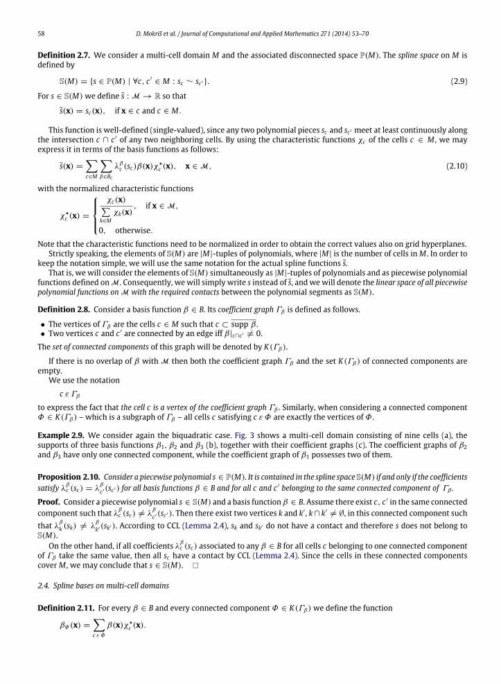
Based on the previous two lemmas and on Corollary 2.13, we are now able to formulate the main result of this appendix.

Theorem A.8. Consider a multi-cell domain M that admits an offset at distance (p − 1)/2, where p is a non-negative integer.Then the p-th combinatorial volume of M— and therefore also the dimension of S(M)— is equal to

ω(p)(M) = z +p2f +

p2

4e +

p3

8v, (A.5)

where z and f are the number of cells and boundary faces, respectively, while the vertex and edge terms v = v0 and e = e0 havebeen defined in Eqs. (A.2) and (A.3).Proof. For even values of p we have that

ω(p)(M) = z(p)

and thus (A.5) follows from Lemma A.6.For odd values of p, we obtain ω(p)(M) = g(M(p−1)). Using Lemma A.7, we obtain

g(M(p−1)) = z(p−1)+

12f (p−1)

+14e(p−1)

+18v(p−1). (A.6)

Using Lemma A.6, Eq. (A.6) implies (A.5). This is where we need the assumption regarding the admissibility of the offset atdistance p−1

2 .According to Corollary 2.13, the combinatorial volume is equal to the dimension of S(M), since the combinatorial volume

is equal to the cardinality of BM and the admissibility of the offset implies the assumption of that corollary.2 Indeed, if thereis a basis function whose coefficient graph has at least two connected components, then we may ‘‘shrink’’ its support to acube s′ consisting of p′

× p′× p′ times cells, where p′

≤ p − 1 is as small as possible, and so that this cube still ‘‘touches’’cells from two components (that is, it contains two points from two different components but (s′) ∩ M

= ∅, see Fig. 11for a bivariate analogy). The center of s′ belongs a self-intersection of the offset at distance p′

2 and thus the offset at distancep−12 is not admissible.

A.3. The case of topological manifolds with boundaries

The remainder of this appendix relates our result to the dimension formula of Berdinsky et al. [25, Corollary 8]. Note thatthis paper also derives other dimension formulas that do not rely on the admissibility of offsets but on other topologicalconstraints [25, Corollary 7].

2 Clearly, the admissibility of the offsets is sufficient but not necessary for this assumption to be satisfied; consider, e.g., uniform triquadratic splines on3 × 3 × 3 cells with the central cell removed.


Fig. 11. If the coefficient graph of a basis function β has two connected components, then shrinking supp β (single hatching) gives a cube s′ (doublehatching) that touches the boundary of M (solid light gray) in at least two disjoint sets of points. The center of s′ (black dot) belongs to a self-intersectionof a certain offset (thick solid black line).

Lemma A.9. For any multi-cell domain M we have that

c + fp2

+ (ecvx − encx − 2eksg)p2

4+ v

p3

8= c(p + 1)3 − fitl p(p + 1)2 + (eitl − eksg)p2(p + 1)

+ (−v4 + v7 + v11 + v12 + 3v13 + v15 + 2v16

+ v18 + v19 − v21)p3 (A.7)

where fitl and eitl are the number of internal faces and internal edges (faces and edges of cells that are contained in the interior ofM), respectively.

Proof. We compare the coefficients of the powers of p on both sides of the equation.p0: We have c = c.p1: We need to prove that

6c = 2fitl + f . (A.8)

This equation is satisfied since each cell has six faces and all internal faces belong to two cells. p2: We need to prove that

3c − 2fitl + eitl − eksg =14(ecvx − encx − 2eksg). (A.9)

Consider the two identities

4f = 2ecvx + 2encx + 4eksg + 2eflt4fitl = 2encx + 4eitl + eflt

where eflt is the number of flat edges, i.e., edges within patches of the boundary of the multi-cell domain (shared by twoco-planar boundary faces). These two identities imply

−4fitl + 2f + 4eitl − 4eksg = ecvx − encx − 2eksg.

Dividing by four and using again (A.8) leads to (A.9). p3: We need to prove that

8(c − fitl + eitl − eksg + (−v4 + v7 + v11 + v12 + 3v13 + v15 + 2v16 + v18 + v19 − v21))

= (v1 − 2v3 − 6v4 − 3v5 − v6 − v7 − 2v9 − 2v10 + 4v13 − v14 + v15 + 3v16 + 2v18 + 2v19 + v20). (A.10)

Each cell has eight vertices, thus

8c = v1 + 2v2 + 2v3 + 2v4 + 3v5 + 3v6 + 3v7 + 4v8 + 4v9

+ 4v10 + 4v11 + 4v12 + 4v13 + 5v14 + 5v15 + 5v16 + 6v17 + 6v18 + 6v19 + 7v20 + 8v21. (A.11)

Similarly, each face has four vertices, hence

4fitl = v2 + v5 + 2v6 + 4v8 + 3v9 + 3v10 + 2v11 + 2v12 + 5v14 + 4v15 + 3v16

+ 7v17 + 6v18 + 6v19 + 9v20 + 12v21.

Moreover, each edge has two vertices, thus

2eitl = v8 + v14 + 2v17 + v18 + 3v20 + 6v21 (A.12)


and

2eksg = v3 + v5 + 3v7 + 2v11 + 2v12 + 6v13 + v15 + 3v16 + v18. (A.13)

A suitable linear combination of (A.11)–(A.13) gives (A.10).

Corollary A.10. Consider a multi-cell domain M with eksg = 0, v4 = 0 and v19 = 0 that admits an offset at distance p−12 . Then

V(p)(M) = c + fp2

+ (ecvx − encx)p2

4+ (v1 − v6 − 2v9 − 2v10 − v14 + v20)

= c(p + 1)3 − fitlp(p + 1)2 + eitlp2(p + 1) − v21p3. (A.14)

Proof. Since eksg = 0, there are no vertices that are incident to a kissing edge, i.e.,

v3 = v5 = v7 = v11 = v12 = v13 = v15 = v16 = v18 = 0.

Substituting these values into (A.7) gives (A.14).

Eq. (A.14) shows that the result of [25, Corollary 8] is a special case of Theorem A.8. Note that a multi-cell domain witheksg = v4 = v19 = 0 is called a topological manifold with boundary in [25].

References

[1] D.R. Forsey, R.H. Bartels, Hierarchical B-spline refinement, Comput. Graph. 22 (1988) 205–212.[2] R. Kraft, Adaptive and linearly independentmultilevel B-splines, in: A. LeMéhauté, C. Rabut, L.L. Schumaker (Eds.), Surface Fitting andMultiresolution

Methods, Vanderbilt University Press, Nashville, 1997, pp. 209–218.[3] G. Greiner, K. Hormann, Interpolating and approximating scattered 3D-data with hierarchical tensor product B-splines, in: A. Le Méhauté, C. Rabut,

L.L. Schumaker (Eds.), Surface Fitting and Multiresolution Methods, in: Innovations in Applied Mathematics, Vanderbilt University Press, Nashville,TN, 1997, pp. 163–172.

[4] J.A. Cottrell, T.J.R. Hughes, Y. Bazilevs, Isogeometric Analysis: Toward Integration of CAD and FEA, John Wiley & Sons, 2009.[5] Y. Bazilevs, V.M. Calo, J.A. Cottrell, J. Evans, T.J.R. Hughes, S. Lipton, M.A. Scott, T.W. Sederberg, Isogeometric analysis using T -splines, Comput. Methods

Appl. Mech. Engrg. 199 (2010) 229–263.[6] M.R. Dörfel, B. Jüttler, B. Simeon, Adaptive isogeometric analysis by local h-refinementwith T -splines, Comput.Methods Appl.Mech. Engrg. 199 (2010)

264–275.[7] T.W. Sederberg, J. Zheng, A. Bakenov, A. Nasri, T -splines and T -NURCCS, ACM Trans. Graph. 22 (2003) 477–484.[8] A.-V. Vuong, C. Giannelli, B. Jüttler, B. Simeon, A hierarchical approach to adaptive local refinement in isogeometric analysis, Comput. Methods Appl.

Mech. Engrg. 200 (2011) 3554–3567.[9] C. Giannelli, B. Jüttler, H. Speleers, THB-splines: the truncated basis for hierarchical splines, Comput. Aided Geom. Design 29 (2012) 485–498.

[10] C. Giannelli, B. Jüttler, H. Speleers, Strongly stable bases for adaptively refined multilevel spline spaces, Adv. Comput. Math. (2014), http://dx.doi.org/10.1007/s10444-013-9315-2, in press.

[11] G. Kiss, C. Giannelli, B. Jüttler, Algorithms and data structures for truncated hierarchical B-splines, in: M. Floater, et al. (Eds.), Mathematical Methodsfor Curves and Surfaces, in: Lecture Notes in Computer Science, vol. 8177, Springer, 2014, pp. 304–323.

[12] P.B. Bornemann, F. Cirak, A subdivision-based implementation of the hierarchical B-spline finite element method, Comput. Methods Appl. Mech.Engrg. 253 (2013) 584–598.

[13] G. Kuru, C.V. Verhoosel, K.G. van der Zeeb, E.H. van Brummelen, Goal-adaptive isogeometric analysis with hierarchical splines, Comput. Methods Appl.Mech. Engrg. 270 (2014) 270–292.

[14] D. Schillinger, L. Dedé, M.A. Scott, J.A. Evans, M.J. Borden, E. Rank, T.J.R. Hughes, An isogeometric design-through-analysis methodology based onadaptive hierarchical refinement of NURBS, immersed boundarymethods, and T -spline CAD surfaces, Comput.Methods Appl.Mech. Engrg. 249 (2012)116–150.

[15] T. Dokken, T. Lyche, K.F. Pettersen, Polynomial splines over locally refined box–partitions, Comput. Aided Geom. Design 30 (2013) 331–356.[16] J. Deng, F. Chen, Y. Feng, Dimensions of spline spaces over T -meshes, J. Comput. Appl. Math. 194 (2006) 267–283.[17] J. Deng, F. Chen, X. Li, Ch. Hu, W. Tong, Z. Yang, Y. Feng, Polynomial splines over hierarchical T -meshes, Graph. Models 70 (2008) 76–86.[18] X. Li, J. Deng, F. Chen, Dimensions of spline spaces over 3D hierarchical T -meshes, J. Inf. Comput. Sci. 3 (2006) 487–501.[19] X. Li, J. Deng, F. Chen, Surface modeling with polynomial splines over hierarchical T -meshes, Vis. Comput. 23 (2007) 1027–1033.[20] X. Li, J. Deng, F. Chen, Polynomial splines over general T -meshes, Vis. Comput. 26 (2010) 277–286.[21] B. Mourrain, On the dimension of spline spaces on planar T -meshes, Math. Comp. 83 (2014) 847–871.[22] K.F. Pettersen, On the dimension of multivariate spline spaces, Report SINTEF A23875, 2013.[23] L.L. Schumaker, L. Wang, Approximation power of polynomial splines on T -meshes, Comput. Aided Geom. Design 29 (2012) 599–612.[24] C. Giannelli, B. Jüttler, Bases and dimensions of bivariate hierarchical tensor-product splines, J. Comput. Appl. Math. 239 (2013) 162–178.[25] D. Berdinsky, T. Kim, C. Bracco, D. Cho, B. Mourrain, M. Oh, S. Kiatpanichgij, Dimensions and bases of hierarchical tensor-product splines, J. Comput.

Appl. Math. 257 (2014) 86–104.[26] D. Berdinsky, T. Kim, D. Cho, C. Bracco, Bases of T -meshes and the refinement of hierarchical B-splines, https://sites.google.com/site/berdinsky/.[27] D. Berdinsky, T. Kim, C. Bracco, D. Cho, M. Oh, Y. Seo, Iterative refinement of hierarchical T -meshes for bases of spline spaces with highest order

smoothness, Comput. Aided Des. 47 (2014) 96–107.[28] H. Prautzsch, W. Boehm, M. Paluszny, Bézier and B-Spline Techniques, Springer, 2002.[29] R. Klette, A. Rosenfeld, Digital Geometry: Geometric Methods for Digital Picture Analysis, Morgan Kaufmann, 2004.

http://refhub.elsevier.com/S0377-0427(14)00182-4/sbref1









http://dx.doi.org/10.1007/s10444-013-9315-2

http://dx.doi.org/10.1007/s10444-013-9315-2

http://dx.doi.org/10.1007/s10444-013-9315-2

http://dx.doi.org/10.1007/s10444-013-9315-2

http://dx.doi.org/10.1007/s10444-013-9315-2

http://dx.doi.org/10.1007/s10444-013-9315-2

http://dx.doi.org/10.1007/s10444-013-9315-2















https://sites.google.com/site/berdinsky/




Documents

On the completeness of hierarchical tensor-product B-splines