Component-aware Tensor-product Trivariate Splines of Arbitrary Topology

Bo Li and Hong Qin

Stony Brook University

Abstract

The fundamental goal of this paper aims to bridge the large gap between the shape versatility of arbitrary topology andthe geometric modeling limitation of conventional tensor-product splines for solid representations. Its contribution liesat a novel shape modeling methodology based on tensor-product trivariate splines for solids with arbitrary topology. Ourframework advocates a divide-and-conquer strategy. The model is first decomposed into a set of components as basicbuilding blocks. Each component is naturally modeled as tensor-product trivariate splines while supporting local refine-ment. The key novelty of this paper is our powerful merging strategy that can glue tensor-product spline solids togethersubject to high-order global continuities. As a result, this new spline representation has many attractive advantages. Atthe theoretical level, the integration of the top-down topological decomposition and the bottom-up spline constructionenables an elegant modeling approach for arbitrary high-genus solids. Each building block is a regular tensor-productspline, which is CAD-ready and facilitates GPU computing. In addition, our new spline merging method enforces thefeatures of semi-standardness (i.e.,

∑

i wi Bi(u, v,w) ≡ 1 everywhere) and boundary restriction (i.e., all blendingfunctionsare confined exactly within parametric domains) in favor of downstream CAE applications. At the computational level,our component-aware spline scheme supports meshless fitting which completely avoids tedious volumetric mapping andremeshing. This divide-and-conquer strategy reduces the time and space complexity drastically. We conduct extensiveexperiments to demonstrate its shape flexibility and versatility towards solid modeling with complicated geometries andnon-trivial genus.

Keywords: Tensor-product splines; Trivariate T-splines; Solid models of arbitrary topology; Semi-standardness;Boundary restriction

1. Introduction and Motivation

The rapid advancement of 3D data-acquisition tech-niques gives rise to a wide variety of tremendous 3D vol-umetric data. Although many 3D representations (e.g.,structured grids or tetrahedral meshes) exhibit variousvirtues for solid modeling and processing, most of theserepresentations are lack of the compactness of smoothlymodeling solid geometry, which is required for CAE, in-cluding both CAGD modeling process and downstreamphysical analysis without data conversion. Therefore, afrequently occurring challenge is how to effectively con-vert a discrete complex volumetric data into a compact andcontinuous spline formulation towards CAE applications.

Our primary goal in this paper is to develop efficientmethods for arbitrary solids undergoing spline transfor-mation. Nevertheless, we must address the followingkey challenges. (1)High genus. An attractive splinerepresentation must accommodate high-genus solid mod-els with complicated shapes. (2)Local refinement andadaptive fitting. For trivariate splines, both structurally-

complicated shape models and feature-enriched modelsneed local refinement. For example, a genus-0 solidbounded by 6 simple four-sided B-spline surfaces hasoriginally 6× 10242 control points (DOFs). The size ofDOFs increases drastically to 10243 or even larger whenwe naively convert it to a volumetric spline representation.This exponential increase during volumetric spline con-version poses a great challenge in terms of both storageand fitting costs. Therefore, it is advantageous to use highresolution to approximate boundary surface and low reso-lution for interior space. (3)Singularity free. A singularpoint in a volumetric domainis a node with valence largerthan four along one iso-parametric plane (Fig. 1(a)). Han-dling singularity with tenor-product splines is highly chal-lenging in FEM, thus a singularity-free domain is highlydesirable. Unfortunately, singularities commonly exist inmany volumetric domains such as hexahedral meshes andcylinder (tube) domains. (4)Boundary restriction. Itis a basic requirement for a spline that all blending func-tions are completely confined within the parametric do-

Preprint submitted to Computer& Graphics April 3, 2009

main. (5)Semi-standardness.A hierarchical spline isalways formulated as Eq. 1. Semi-standardness, meaningthat∑B

i=1 wi Bi(u, v,w) ≡ 1 always holds for all (u, v,w),has a broader appeal to both theoreticians and practition-ers.

(a) (b) (c)

Figure 1: (a) The singular point in the volumetric domain. (b-c) A poly-cube domain can mimic the geometry of input and avoid such type ofsingular point.

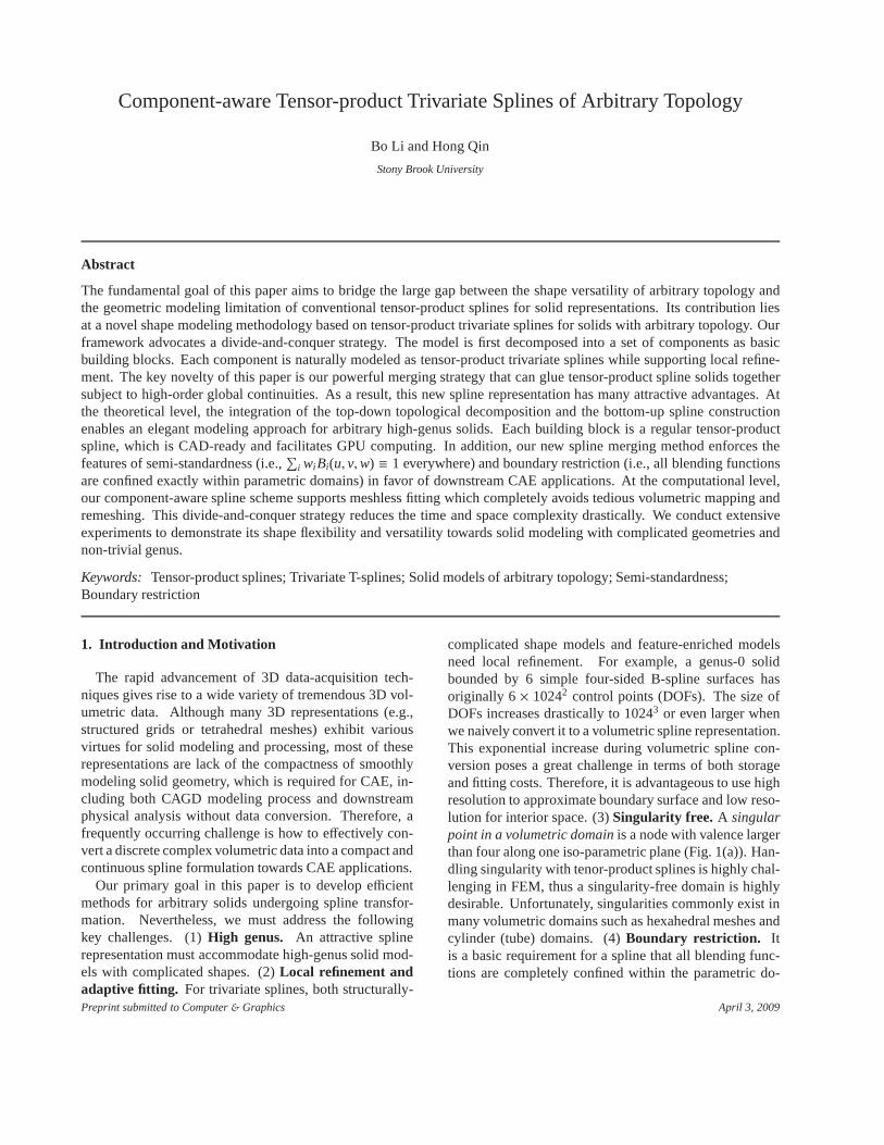
Recently, much work has been attempted towards splinemodeling of arbitrary topology shape while satisfying theaforementioned requirements, following a top-down fash-ion like Wang et al.[1]. They have proposed a theoreti-cal trivariate spline scheme, being built upon volumetricpoly-cube domains. Poly-cube is a shape composed ofcuboids that abut with each other. All cuboids are gluedin various merging types like Fig. 2, without any singu-lar point (Note that the yellow dots arenotsingular pointsin the trivariate splines, even though they are singular forsurface study). For example, a poly-cube parametric do-main like Fig. 1(c) is designed to mimic shape geometryFig. 1(b). Although their spline refinement guarantees thefeatures such as semi-standardness and boundary restric-tion, this theoretical formulation encounters many diffi-culties. A global one-piece poly-cube domain, togetherwith its 3D embedding, is not versatile enough to handlehighly-twisted and high-genus solid datasets. Creating apoly-cube to mimic the input shape requires tedious userwork. The boundary restriction procedure in the vincinityof gluing regions (Fig. 2, yellow dots/lines) is extremelycomplicated. Computationally speaking, the global fittingis very time consuming which is completely unsuitable fortrivariate splines.

(a) (b) (c) (d)

Figure 2: All possible merging types in a poly-cube (“Type-1” to “Type-4”). To preserve both boundary restriction and semi-standardness, weadd extra knots around the control points on the merging boundary (yel-low lines and dots).

To ameliorate, our framework takes advantage of the

bottom-up scheme. The global domain is divided into sev-eral components, with a controllable number and typesof the cuboid merging. We build tensor-product trivari-ate splines separately for each component, and then gluethem together. Compared with the top-down scheme, ourdivide-and-conquer method is more flexible and power-ful to handle high-genus and complex shape. The interiorspace mapping and remeshing in each component is mucheasier. Compared with global fitting, our local fitting re-duces both the computation time and space consumptionsignificantly.

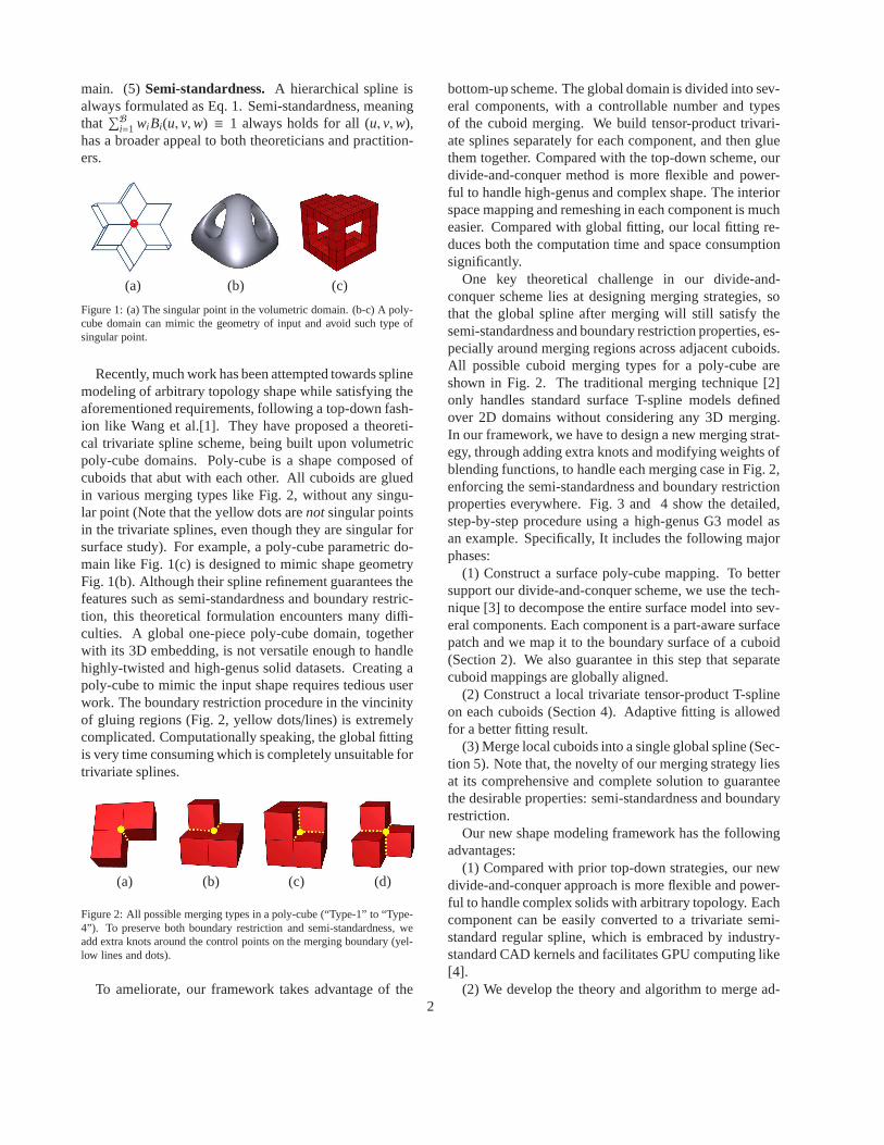
One key theoretical challenge in our divide-and-conquer scheme lies at designing merging strategies, sothat the global spline after merging will still satisfy thesemi-standardness and boundary restriction properties, es-pecially around merging regions across adjacent cuboids.All possible cuboid merging types for a poly-cube areshown in Fig. 2. The traditional merging technique [2]only handles standard surface T-spline models definedover 2D domains without considering any 3D merging.In our framework, we have to design a new merging strat-egy, through adding extra knots and modifying weights ofblending functions, to handle each merging case in Fig. 2,enforcing the semi-standardness and boundary restrictionproperties everywhere. Fig. 3 and 4 show the detailed,step-by-step procedure using a high-genus G3 model asan example. Specifically, It includes the following majorphases:

(1) Construct a surface poly-cube mapping. To bettersupport our divide-and-conquer scheme, we use the tech-nique [3] to decompose the entire surface model into sev-eral components. Each component is a part-aware surfacepatch and we map it to the boundary surface of a cuboid(Section 2). We also guarantee in this step that separatecuboid mappings are globally aligned.

(2) Construct a local trivariate tensor-product T-splineon each cuboids (Section 4). Adaptive fitting is allowedfor a better fitting result.

(3) Merge local cuboids into a single global spline (Sec-tion 5). Note that, the novelty of our merging strategy liesat its comprehensive and complete solution to guaranteethe desirable properties: semi-standardness and boundaryrestriction.

Our new shape modeling framework has the followingadvantages:

(1) Compared with prior top-down strategies, our newdivide-and-conquer approach is more flexible and power-ful to handle complex solids with arbitrary topology. Eachcomponent can be easily converted to a trivariate semi-standard regular spline, which is embraced by industry-standard CAD kernels and facilitates GPU computing like[4].

(2) We develop the theory and algorithm to merge ad-2

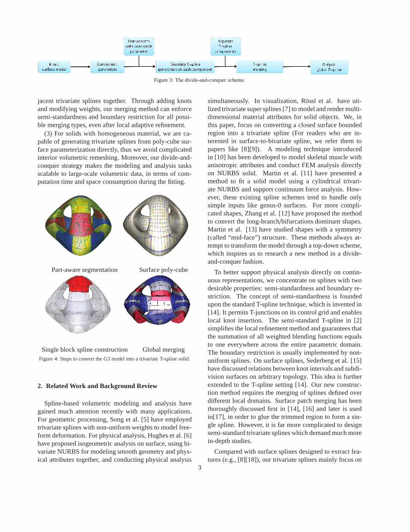
Figure 3: The divide-and-conquer scheme.

jacent trivariate splines together. Through adding knotsand modifying weights, our merging method can enforcesemi-standardness and boundary restriction for all possi-ble merging types, even after local adaptive refinement.

(3) For solids with homogeneous material, we are ca-pable of generating trivariate splines from poly-cube sur-face parameterization directly, thus we avoid complicatedinterior volumetric remeshing. Moreover, our divide-and-conquer strategy makes the modeling and analysis tasksscalable to large-scale volumetric data, in terms of com-putation time and space consumption during the fitting.

Part-aware segmentation Surface poly-cube

Single block spline construction Global mergingFigure 4: Steps to convert the G3 model into a trivariate T-spline solid.

2. Related Work and Background Review

Spline-based volumetric modeling and analysis havegained much attention recently with many applications.For geometric processing, Song et al. [5] have employedtrivariate splines with non-uniform weights to model free-form deformation. For physical analysis, Hughes et al. [6]have proposed isogeometric analysis on surface, using bi-variate NURBS for modeling smooth geometry and phys-ical attributes together, and conducting physical analysis

simultaneously. In visualization, Rossl et al. have uti-lized trivariate super splines [7] to model and render multi-dimensional material attributes for solid objects. We, inthis paper, focus on converting a closed surface boundedregion into a trivariate spline (For readers who are in-terested in surface-to-bivariate spline, we refer them topapers like [8][9]). A modeling technique introducedin [10] has been developed to model skeletal muscle withanisotropic attributes and conduct FEM analysis directlyon NURBS solid. Martin et al. [11] have presented amethod to fit a solid model using a cylindrical trivari-ate NURBS and support continuum force analysis. How-ever, these existing spline schemes tend to handle onlysimple inputs like genus-0 surfaces. For more compli-cated shapes, Zhang et al. [12] have proposed the methodto convert the long-branch/bifurcations dominant shapes.Martin et al. [13] have studied shapes with a symmetry(called “mid-face”) structure. These methods always at-tempt to transform the model through a top-down scheme,which inspires us to research a new method in a divide-and-conquer fashion.

To better support physical analysis directly on contin-uous representations, we concentrate on splines with twodesirable properties: semi-standardness and boundary re-striction. The concept of semi-standardness is foundedupon the standard T-spline technique, which is invented in[14]. It permits T-junctions on its control grid and enableslocal knot insertion. The semi-standard T-spline in [2]simplifies the local refinement method and guarantees thatthe summation of all weighted blending functions equalsto one everywhere across the entire parametric domain.The boundary restriction is usually implemented by non-uniform splines. On surface splines, Sederberg et al. [15]have discussed relations between knot intervals and subdi-vision surfaces on arbitrary topology. This idea is furtherextended to the T-spline setting [14]. Our new construc-tion method requires the merging of splines defined overdifferent local domains. Surface patch merging has beenthoroughly discussed first in [14], [16] and later is usedin[17], in order to glue the trimmed region to form a sin-gle spline. However, it is far more complicated to designsemi-standard trivariate splines which demand much morein-depth studies.

Compared with surface splines designed to extract fea-tures (e.g., [8][18]), our trivariate splines mainly focuson

3

finding part-aware component structures. Besides poly-cube domains, another commonly-used part-aware do-main is cylinder (tube) like [11]. Martin et al. in [13] haveextended this domain to mimic more complex shapes.However, in terms of spline construction, the cylinder(tube) domain inevitably produces singular points alongthe tube axis. Handling singularity with still high-ordercontinuity is extremely difficult in spline research. Forsurface modeling, Loop and Scheafer in [19] have givenan example of aG2 polynomial construction with generalconnectivity to accommodate singularities. On the otherhand, Peters and Fan [20] have introduced rational linearmaps to replace affine linear atlas and handle singulari-ties between charts. We observe that poly-cube uses part-aware cuboids as building block and avoids any singular-ities. Thus it serves very well as the trivariate spline do-main. It is pioneered by [21] for seamless texture mappingand can be used as a parametric domain for spline con-struction like in [9]. However, although poly-cube domaincan be constructed in an automatic fashion like [22][23],in practice, users may have to rely on manual construc-tion for fine quality control and model refinement. Themain challenges include how to detect and decompose theinput into part-aware components, and connect these com-ponents in a regular/singular-free way.

Conventionally, when converting a surface input to aspline-ready format, the first step is meshing or remesh-ing the interior volume into a tetrahedral mesh (like [24])or any other format (like [25]). Then we compute thevolumetric parameterization on the remeshing result. Afew recent works [13][26][27] have studied the volumet-ric parameterization calculated on the tetrahedral mesh.They typically start from a surface mapping as the bound-ary constraint. These interior mapping methods alwaysinvolve time-consuming numerical procedures. It wouldbe intriguing to ask whether we could better embed vol-umetric mapping step into our whole spline-based modeltransformation framework.

3. Component Generation and T-splines

This section briefly reviews the required surface poly-cube generation algorithm. We also define the necessarynotations for the rest of the paper. In the interest of un-derstanding, most illustrative figures about knots are sim-ply shown in 2D layout, as their 3D generalizations arestraightforward.

3.1. Component Generation

The starting point of our whole procedure is to decom-pose an input surface model into several component sur-face. Each component surface is part-aware and maps toa cuboid surface. The decomposition and mapping must

follow the rule that parameters between neighboring com-ponents are consistent (i.e., we can glue their parameterstogether directly as a seamless aligned global poly-cubemapping). We remain agnostic as to which method shouldbe used for such decomposition. However, in order to bet-ter promise these requirements, we utilize the algorithm[3] for this step. The algorithm is briefly summarized hereas the resulting cuboid-connecting structure is essentialfor introducing our spline merging algorithm. The algo-rithm proceeds in several steps:

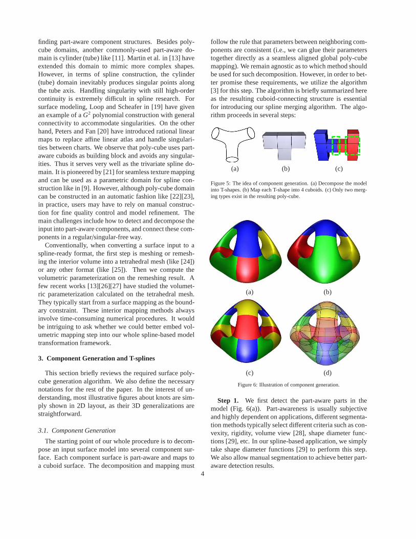
(a) (b) (c)

Figure 5: The idea of component generation. (a) Decompose the modelinto T-shapes. (b) Map each T-shape into 4 cuboids. (c) Only two merg-ing types exist in the resulting poly-cube.

(a) (b)

(c) (d)

Figure 6: Illustration of component generation.

Step 1. We first detect the part-aware parts in themodel (Fig. 6(a)). Part-awareness is usually subjectiveand highly dependent on applications, different segmenta-tion methods typically select different criteria such as con-vexity, rigidity, volume view [28], shape diameter func-tions [29], etc. In our spline-based application, we simplytake shape diameter functions [29] to perform this step.We also allow manual segmentation to achieve better part-aware detection results.

4

Step 2.We attempt to generate a group of T-shapes likeFig. 5(a). Note that the resulting decomposed patches arealways connected irregularly and not singularity free (i.e.,not connected as regularly as cuboids in a poly-cube). Were-segment and group the patches into unified componentswith simple connections (Fig. 6(b)): (1) For each patchwith a torus, we generate the shortest handle path [30] andcut along the path. (2) For each patch withn boundaries(n > 3), we choose 2 boundaries (a pair with the closestdistance) and then generate a bounding loop as in [31].We cut along the loop, generating a 3-boundary patch anda (n− 1)-boundary patch. We iteratively execute this stepuntil all resulting patches have 3 boundaries. (3) For eachpatch with 1 or 2 boundaries (like a “tube” shape), wemerge this patch into a connected 3 boundary patch. Wecan also split a “tube” into two if it is much longer thanother patches. After this procedure, the resulting patchhas 3 boundaries and geometrically similar to a volumetric“T” ( “T-shape”) like Fig. 5(a).

Step 3.In order to transform a T-shape to 4 cuboids likeFig. 5(b), we trace curves on every T-shape. These curvescut each T-shape into 4 patches (Fig. 6(c)). The resultingpatch may include several cutting boundaries and we fillthem by [32], converting the patch into a closed genus-0surface. Each patch is bounded by 12 curves and they willbe mapped onto the cuboid domain edges (Thus we callthese curves“poly-edges”, like grey lines in Fig. 6(d)).Note that the poly-edges between two connected cuboidpatches are aligned, thus their parameters on the commonboundary are identical, which (1) guarantees our poly-cube mapping is a globally-aligned parametrization (2)enables in the next step two spline volume patches canbe merged together with no distortion.

Step 4. We map each patch to a cuboid surface(Fig. 4(b)). We first map the 12 poly-edges onto cuboidedges. Then we use this mapping as the constraint andcompute 3 harmonic equations∆u = 0,∆v = 0,∆w = 0.In practice, we solve every equation on the discrete trian-gle mesh by mean value coordinates [33]. We also lo-cally modify the coordinates along boundaries betweentwo connected patches to keep the parameters aligned andconsistent.

Advantages. Compared with the conventional poly-cube mapping method like [21], our construction is specif-ically suitable for the divide-and-conquer strategy andspline construction. (1) The conventional poly-cubemethod always generates an integral poly-cube domain tomimic the whole shape at first. Then we have to decom-pose this integral domain into small pieces for applyingthe divide-and-conquer strategy. In contrast, our methoddirectly uses a small set of connected local cuboids, eachof which represents a geometrically meaningful patch(e.g., part-aware). This property is particularly suitable for

highly-twisted/non-axis aligned/high-genus models (e.g.,the g3 model). More importantly, we can use the divide-and-conquer technique directly on our resulting poly-cubewithout further decomposing anymore. (2) Our methodcan also reduce the number of cuboids, and control themerging types efficiently: as shown in Fig. 5(c), it onlygenerates “Two-cube” and“Type-1” (Fig. 2(a)) merging,thus it simplifies the merging requirement.

3.2. Trivariate T-spline

To better prepare readers for the better understanding ofthe following algorithm, we briefly define the volumetricT-spline representation (The surface T-spline formulationis detailed in [2]). Also we give the detailed explanationof “Semi-standardness”and ”Boundary Restriction”asfollows.

We useT(V,F ,C) (or simply T) to denote a controlgrid domain, whereV,F , andC are sets of vertices, facesand cells, respectively. GivenT, a trivariate T-spline canbe formulated as:

F(u, v,w) =

∑Bi=1 wipi Bi(u, v,w)∑B

i=1 wi Bi(u, v,w), (1)

where (u, v,w) denotes parametric coordinates,pi is a con-trol point,W andB are the weight and blending functionsets. Each pair of< wi Bi > is associated with a controlpointpi . EachBi(u, v,w) ∈ B is a blending function:

Bi(u, v,w) = N3i0(u)N3

i1(v)N3i2(w), (2)

whereN3i0(u), N3

i1(v) andN3i2(w) are cubic B-spline basis

functions alongu, v,w, respectively.In the case of cubic T-spline blending functions in Eq. 1,

the univariate functionN3j for each blending functionBi

is constructed upon knot vectorRj = [r j−2, r

j−1, r

j0, r

j1, r

j2],

whereRj is a tracing ray parallel to the control grid (SeeFig. 7(b)): Starting from a knotk = r0

0, r10, r

20, we can trace

to r01 andr0

−1, which are the very first intersections whenthe rayR(t) = (r0

0 ± t, r10, r

20) comes across one cell face.

Naturally, we define the parameter of a control point asthe central knot of the knot sequence for the control point.

To support downstream CAE applications, our splineframework has the following requirements:Semi-standardness.

∑Bi=1 wi Bi(u, v,w) ≡ 1 holds for all

(u, v,w) in Eq. 1, so that the evaluation of spline functionsand their derivatives is both efficient and stable. Eq. 1 canbe rewritten as:

F(u, v,w) =B∑

i=1

wipi Bi(u, v,w), (3)

Boundary restriction. We require that blending func-tions of all control points are strictly confined within para-metric domain boundaries. Unfortunately, achieving this

5

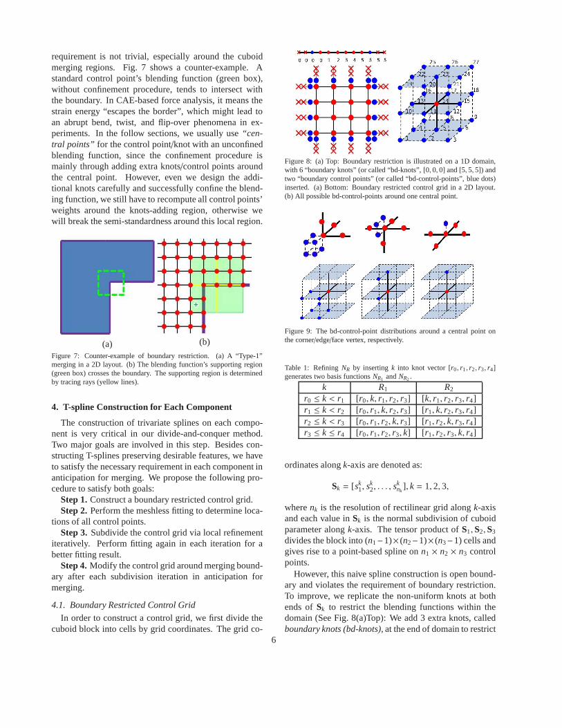
requirement is not trivial, especially around the cuboidmerging regions. Fig. 7 shows a counter-example. Astandard control point’s blending function (green box),without confinement procedure, tends to intersect withthe boundary. In CAE-based force analysis, it means thestrain energy “escapes the border”, which might lead toan abrupt bend, twist, and flip-over phenomena in ex-periments. In the follow sections, we usually use“cen-tral points” for the control point/knot with an unconfinedblending function, since the confinement procedure ismainly through adding extra knots/control points aroundthe central point. However, even we design the addi-tional knots carefully and successfully confine the blend-ing function, we still have to recompute all control points’weights around the knots-adding region, otherwise wewill break the semi-standardness around this local region.

(a) (b)

Figure 7: Counter-example of boundary restriction. (a) A “Type-1”merging in a 2D layout. (b) The blending function’s supporting region(green box) crosses the boundary. The supporting region is determinedby tracing rays (yellow lines).

4. T-spline Construction for Each Component

The construction of trivariate splines on each compo-nent is very critical in our divide-and-conquer method.Two major goals are involved in this step. Besides con-structing T-splines preserving desirable features, we haveto satisfy the necessary requirement in each component inanticipation for merging. We propose the following pro-cedure to satisfy both goals:

Step 1.Construct a boundary restricted control grid.Step 2.Perform the meshless fitting to determine loca-

tions of all control points.Step 3.Subdivide the control grid via local refinement

iteratively. Perform fitting again in each iteration for abetter fitting result.

Step 4.Modify the control grid around merging bound-ary after each subdivision iteration in anticipation formerging.

4.1. Boundary Restricted Control Grid

In order to construct a control grid, we first divide thecuboid block into cells by grid coordinates. The grid co-

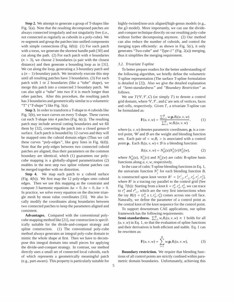
Figure 8: (a) Top: Boundary restriction is illustrated on a 1D domain,with 6 “boundary knots” (or called “bd-knots”, [0, 0, 0] and [5, 5, 5]) andtwo “boundary control points” (or called “bd-control-points”, blue dots)inserted. (a) Bottom: Boundary restricted control grid in a2D layout.(b) All possible bd-control-points around one central point.

Figure 9: The bd-control-point distributions around a central point onthe corner/edge/face vertex, respectively.

Table 1: RefiningNR by insertingk into knot vector [r0, r1, r2, r3, r4]generates two basis functionsNR1 andNR2 .

k R1 R2

r0 ≤ k < r1 [r0, k, r1, r2, r3] [k, r1, r2, r3, r4]r1 ≤ k < r2 [r0, r1, k, r2, r3] [r1, k, r2, r3, r4]r2 ≤ k < r3 [r0, r1, r2, k, r3] [r1, r2, k, r3, r4]r3 ≤ k ≤ r4 [r0, r1, r2, r3, k] [r1, r2, r3, k, r4]

ordinates alongk-axis are denoted as:

Sk = [sk1, s

k2, . . . , s

knk

], k = 1, 2, 3,

wherenk is the resolution of rectilinear grid alongk-axisand each value inSk is the normal subdivision of cuboidparameter alongk-axis. The tensor product ofS1,S2,S3

divides the block into (n1−1)× (n2−1)× (n3−1) cells andgives rise to a point-based spline onn1 × n2 × n3 controlpoints.

However, this naive spline construction is open bound-ary and violates the requirement of boundary restriction.To improve, we replicate the non-uniform knots at bothends ofSk to restrict the blending functions within thedomain (See Fig. 8(a)Top): We add 3 extra knots, calledboundary knots (bd-knots), at the end of domain to restrict

6

the boundary. The knot set is expanded:

Sk = [sk1, s

k1, s

k1, s

k1, s

k2, . . . , s

knk, sk

nk, sk

nk, sk

nk].

We also add 1 extraboundary control point (bd-control-point) (blue dots), on the bd-knot outside of the last con-trol point on the boundary. Fig. 8(a)Bottom extends it toa 2D domain, and its extension to the 3D domain is in thesame pattern. Our spline definition achieves: (1) now ev-ery blending function in each domain is confined withinthe domain boundary; (2) only bd-control-points’ blend-ing functions influence the cuboid boundary, so our fol-lowing fitting method can rely on this usable property.

In order to represent the bd-control-points conveniently,we can arrange them into a 3×3×3 grid around the centralpoint as Fig. 8(b) (recall that the central point is the con-trol point with an unconfined blending function). These27 possible knots share the same parameters as the centralpoint. It is only designed to explicitly record topologicalrelations of these control points in preparation for efficientspline merging. After adding bd-control-points to the 3Dcontrol grid, each central point on the corner/edge/facehas8/4/2 control points, respectively (Fig. 9). This special bd-control-point representation is uniquely suitable for merg-ing processing as shown in Section 5.

4.2. Meshless Fitting

Our input only includes a control grid and a group ofsurface sample points extracted from the surface patch (al-ready mapped to a cuboid domain surface). The challengeconsists in designing a fitting method for solids withoutinterior volumetric parameterization or remeshing.

Step 1. Boundary fitting. We first determine the po-sitions of bd-control-points only. Recall that only bd-control-pointspb

i influence the cuboid surface samplepoints. Therefore, we can determine their positions byminimizing Eq. 4 w.r.t. to surface sample pointvb

j :

argmin(m∑

j=1

||F( f −1(vbj )) − vb

j ||) (4)

⇒∂

∂pbi

m∑

j=1

(F( f −1(vbj )) − vb

j )2

where F denotes the spline function as Eq. 1 andf −1(vb

j ) the parameters ofvbj in the cuboid. The above

equation can be rewritten in matrix format as in the leastsquarex method:

12

PTBTBP− VTBP = 0, (5)

where B is the matrix of blending functionsBi j =

I3×3Bi( f −1(vbj )), V and P denote the vectors of surface

sample pointsvbj and bd-control-pointspb

i , respectively.This equation determines bd-control-points and they serveas the constraint in the next interior fitting step.

Step 2. Interior fitting. Let u in the setU be the in-terior parametric value. Eachui = (u, v,w) is the inte-rior parameter triplet in the tensor-product parametric grid(u0, u1, . . . , un0)× (v0, v1, . . . , vn1)× (w0,w1, . . . ,wn1). The-oretically, we have the following harmonic equation w.r.t.interior control pointspin

j :

argmin(m∑

i=1

∫

Ωi

||∇ · ∇F(ui)||du) (6)

⇒∂

∂pinj

m∑

i=1

∫

Ωi

(4F(ui))2du = 0,

whereΩi is an infinitesimal parametric volume aroundui .Similar as [34], the above minimized energy

∫

Ωi||4F(ui)||

can be approximated by the following formulation:

m∑

j=0

wi j F(u j) = 0,wi j =

1 i = j,− 1

6 u j ∈ Nbr (ui)0 others

(7)

whereNbr includes 6 immediate neighbors ofui in thetensor-product parametric grid. We substitute Eq. 7 intoEq. 6, which can be solved by the least square methodsimilar to Eq. 4. During computing we set already-knownpb

i as constraints and get all other control point positions.Global alignment. Although we execute volumetric

fitting separately on every cuboid, our fitting techniquestill guarantees global alignment of interior fitting results.Recall that we already obtain the identical surface param-eters between cuboids before fitting, since we generatealigned poly-edges (i.e., cuboid edges). Therefore, twocuboids minimize precisely the same energy in Eq. 4 andEq. 6 on the boundary, leading to the equivalent fitting re-sults.

4.3. Cell Subdivision and Local Refinement

If the fitting results do not meet certain criteria on eachcuboid, we can always perform subdivision over cells inthe control grid with large fitting errors and then conductthe volumetric fitting. Each cell is split along 3-axis anddivided into eight sub-cells naturally.

The challenge is how to preserve the semi-standardnessduring subdivision. Sederberg et al. [2] have proposed afeasible approach to refine blending functions on surfacepatch. We generalize this technique onto our 3D controlgrid. LetR= [r0, r1, r2, r3, r4] be a ray-tracing knot vectorandNR(u) denotes the corresponding cubic B-spline basisfunction. If there is an additional knotk ∈ [r0, r4] inserted

7

into R, N can be written as a linear combination of twoB-spline functions:

NR(u) = c1NR1(u) + c2NR2(u). (8)

Two knot vectorsR1,R2 are shown in Table 1,c1 andc2

are 2 weights that can not exceed 1:

c1 = min(k− r0

r3 − r0, 1), c2 = min(

r4 − kr4 − r1

, 1).

Since the blending function ofB is the tensor product ofNalong 3-axis, we can also formulate the refined blendingfunctions along one axis:

Bi ≡ c1Bi1 + c2Bi2. (9)

The procedure of our 3D subdivision and local refine-ment consists of following steps. The input is a queue ofcell Qc.

Step 1.Subdivide cells inQc and insert the new verticesinto the domainT, and updateT to T∗

Step 2. For all pairs of blending functions< wi Bi >

,wi ∈ W, Bi ∈ B, compute its new knot vectorR∗ (SeeSection 3). Then,

• If the R∗ includes the knot which does not exist inT∗,insert a new vertex on that knot into the domainT∗.

• If the R∗ is more refined thanR, compute the refine-mentBi = c1×Bi1+c2×Bi2. Insert the new blendingfunctions< wi × c1Bi1 > and< wi × c2Bi2 > into thecontrol grid. Delete the old pair< wi Bi >.

Step 3.Repeat the last step until no new knot vector inR∗.Collect all blending functions on the same control pointand use the total weight as its new weight.

The above procedure can handle refinement and knotextraction on a complicated 3D control grid. It also deter-mines new required control points automatically to guar-antee the semi-standardness. Note that unlike [2], we per-form spline fitting again after each refinement iteration toupdate control point positions. This is mainly because ourgoal of refinement is to seek for more accurate fitting re-sult. In contrast, the refinement in [2] aims to keep theshape unchanged.

4.4. Boundary Modification

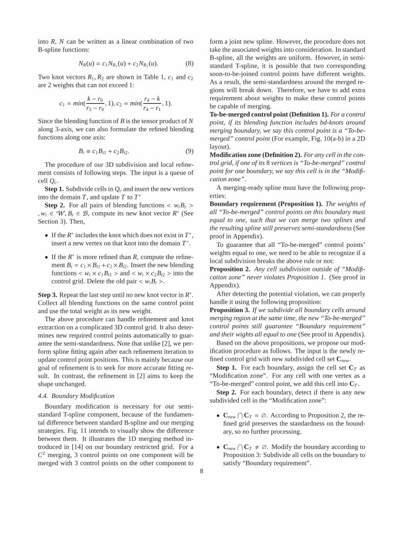
Boundary modification is necessary for our semi-standard T-spline component, because of the fundamen-tal difference between standard B-spline and our mergingstrategies. Fig. 11 intends to visually show the differencebetween them. It illustrates the 1D merging method in-troduced in [14] on our boundary restricted grid. For aC2 merging, 3 control points on one component will bemerged with 3 control points on the other component to

form a joint new spline. However, the procedure does nottake the associated weights into consideration. In standardB-spline, all the weights are uniform. However, in semi-standard T-spline, it is possible that two correspondingsoon-to-be-joined control points have different weights.As a result, the semi-standardness around the merged re-gions will break down. Therefore, we have to add extrarequirement about weights to make these control pointsbe capable of merging.To-be-merged control point (Definition 1).For a controlpoint, if its blending function includes bd-knots aroundmerging boundary, we say this control point is a “To-be-merged” control point(For example, Fig. 10(a-b) in a 2Dlayout).Modification zone (Definition 2).For any cell in the con-trol grid, if one of its8 vertices is “To-be-merged” controlpoint for one boundary, we say this cell is in the “Modifi-cation zone”.

A merging-ready spline must have the following prop-erties:Boundary requirement (Proposition 1). The weights ofall “To-be-merged” control points on this boundary mustequal to one, such that we can merge two splines andthe resulting spline still preserves semi-standardness(Seeproof in Appendix).

To guarantee that all “To-be-merged” control points’weights equal to one, we need to be able to recognize if alocal subdivision breaks the above rule or not:Proposition 2. Any cell subdivision outside of “Modifi-cation zone” never violates Proposition 1.(See proof inAppendix).

After detecting the potential violation, we can properlyhandle it using the following proposition:Proposition 3. If we subdivide all boundary cells aroundmerging region at the same time, the new “To-be-merged”control points still guarantee “Boundary requirement”and their wights all equal to one(See proof in Appendix).

Based on the above propositions, we propose our mod-ification procedure as follows. The input is the newly re-fined control grid with new subdivided cell setCnew.

Step 1. For each boundary, assign the cell setCT as“Modification zone”. For any cell with one vertex as a“To-be-merged” control point, we add this cell intoCT .

Step 2. For each boundary, detect if there is any newsubdivided cell in the “Modification zone”:

• Cnew⋂

CT = ∅. According to Proposition 2, the re-fined grid preserves the standardness on the bound-ary, so no further processing.

• Cnew⋂

CT , ∅. Modify the boundary according toProposition 3: Subdivide all cells on the boundary tosatisfy “Boundary requirement”.

8

Step 3. Update control point positions. Instead of fit-ting again like in Section 4.3, we use the same methodas in [2] because we seek for keeping spline shape un-changed in this step.

(a) (b)

(c) (d)

Figure 10: Boundary modification. (a) Original “To-be-merged” controlpoints (in the green box). (b) Subdivision all cells along the bound-ary, according to Proposition 3. The green box covers updated “To-be-merged” control points. (c) and (d) “Modification zone” (green box) of(a) and (b). According to Proposition 2, cell subdivision (by green dots)outside “Modification zone” does not violate “Boundary requirement”(Proposition 1).

5. Global Merging Strategies

In our framework, the decomposed components can bemerged in various different merging types. We develop al-gorithms to handle different types of merging in this sec-tion. As we discussed in Section 3.1, our domain onlyincludes “Two-cube” merging (Section 5.1) and “Type-1” merging (Section 5.2). Also, we seek to handle morecomplicated conventional poly-cube domains, includingall other types of merging in Fig. 2 (Section 5.3).

Figure 11: Two cube merging in 1D layout. Two control points are com-bined to form one new control point (4, 5 and 6).

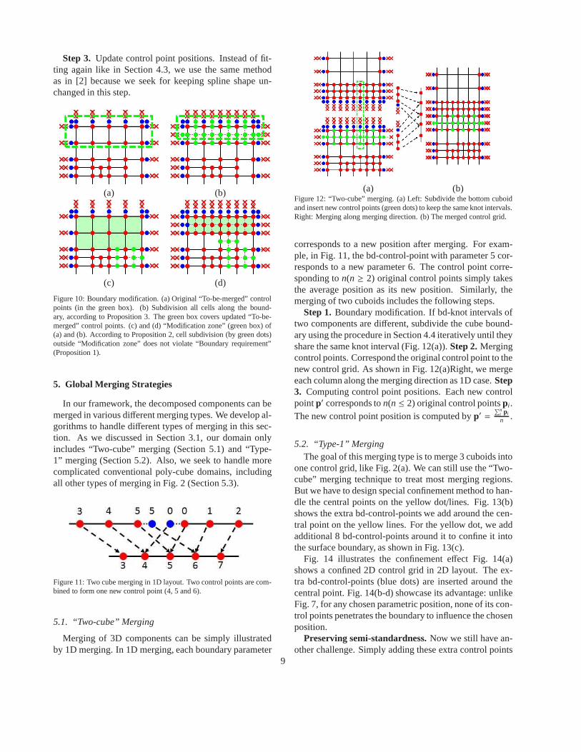
5.1. “Two-cube” Merging

Merging of 3D components can be simply illustratedby 1D merging. In 1D merging, each boundary parameter

(a) (b)Figure 12: “Two-cube” merging. (a) Left: Subdivide the bottom cuboidand insert new control points (green dots) to keep the same knot intervals.Right: Merging along merging direction. (b) The merged control grid.

corresponds to a new position after merging. For exam-ple, in Fig. 11, the bd-control-point with parameter 5 cor-responds to a new parameter 6. The control point corre-sponding ton(n ≥ 2) original control points simply takesthe average position as its new position. Similarly, themerging of two cuboids includes the following steps.

Step 1.Boundary modification. If bd-knot intervals oftwo components are different, subdivide the cube bound-ary using the procedure in Section 4.4 iteratively until theyshare the same knot interval (Fig. 12(a)).Step 2.Mergingcontrol points. Correspond the original control point to thenew control grid. As shown in Fig. 12(a)Right, we mergeeach column along the merging direction as 1D case.Step3. Computing control point positions. Each new controlpointp′ corresponds ton(n ≤ 2) original control pointspi .The new control point position is computed byp′ =

∑ni pi

n .

5.2. “Type-1” MergingThe goal of this merging type is to merge 3 cuboids into

one control grid, like Fig. 2(a). We can still use the “Two-cube” merging technique to treat most merging regions.But we have to design special confinement method to han-dle the central points on the yellow dot/lines. Fig. 13(b)shows the extra bd-control-points we add around the cen-tral point on the yellow lines. For the yellow dot, we addadditional 8 bd-control-points around it to confine it intothe surface boundary, as shown in Fig. 13(c).

Fig. 14 illustrates the confinement effect Fig. 14(a)shows a confined 2D control grid in 2D layout. The ex-tra bd-control-points (blue dots) are inserted around thecentral point. Fig. 14(b-d) showcase its advantage: unlikeFig. 7, for any chosen parametric position, none of its con-trol points penetrates the boundary to influence the chosenposition.

Preserving semi-standardness.Now we still have an-other challenge. Simply adding these extra control points

9

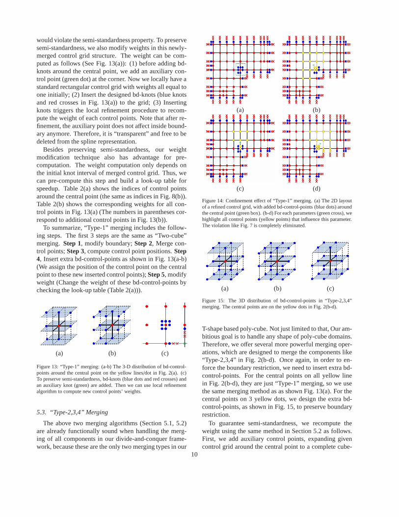
would violate the semi-standardness property. To preservesemi-standardness, we also modify weights in this newly-merged control grid structure. The weight can be com-puted as follows (See Fig. 13(a)): (1) before adding bd-knots around the central point, we add an auxiliary con-trol point (green dot) at the corner. Now we locally have astandard rectangular control grid with weights all equal toone initially; (2) Insert the designed bd-knots (blue knotsand red crosses in Fig. 13(a)) to the grid; (3) Insertingknots triggers the local refinement procedure to recom-pute the weight of each control points. Note that after re-finement, the auxiliary point does not affect inside bound-ary anymore. Therefore, it is “transparent” and free to bedeleted from the spline representation.

Besides preserving semi-standardness, our weightmodification technique also has advantage for pre-computation. The weight computation only depends onthe initial knot interval of merged control grid. Thus, wecan pre-compute this step and build a look-up table forspeedup. Table 2(a) shows the indices of control pointsaround the central point (the same as indices in Fig. 8(b)).Table 2(b) shows the corresponding weights for all con-trol points in Fig. 13(a) (The numbers in parentheses cor-respond to additional control points in Fig. 13(b)).

To summarize, “Type-1” merging includes the follow-ing steps. The first 3 steps are the same as “Two-cube”merging. Step 1, modify boundary;Step 2, Merge con-trol points;Step 3, compute control point positions.Step4, Insert extra bd-control-points as shown in Fig. 13(a-b)(We assign the position of the control point on the centralpoint to these new inserted control points);Step 5, modifyweight (Change the weight of these bd-control-points bychecking the look-up table (Table 2(a))).

(a) (b) (c)

Figure 13: “Type-1” merging: (a-b) The 3-D distribution of bd-control-points around the central point on the yellow lines/dot in Fig. 2(a). (c)To preserve semi-standardness, bd-knots (blue dots and redcrosses) andan auxiliary knot (green) are added. Then we can use local refinementalgorithm to compute new control points’ weights.

5.3. “Type-2,3,4” Merging

The above two merging algorithms (Section 5.1, 5.2)are already functionally sound when handling the merg-ing of all components in our divide-and-conquer frame-work, because these are the only two merging types in our

(a) (b)

(c) (d)

Figure 14: Confinement effect of “Type-1” merging. (a) The 2D layoutof a refined control grid, with added bd-control-points (blue dots) aroundthe central point (green box). (b-d) For each parameters (green cross), wehighlight all control points (yellow points) that influencethis parameter.The violation like Fig. 7 is completely eliminated.

(a) (b) (c)

Figure 15: The 3D distribution of bd-control-points in “Type-2,3,4”merging. The central points are on the yellow dots in Fig. 2(b-d).

T-shape based poly-cube. Not just limited to that, Our am-bitious goal is to handle any shape of poly-cube domains.Therefore, we offer several more powerful merging oper-ations, which are designed to merge the components like“Type-2,3,4” in Fig. 2(b-d). Once again, in order to en-force the boundary restriction, we need to insert extra bd-control-points. For the central points on all yellow linein Fig. 2(b-d), they are just “Type-1” merging, so we usethe same merging method as as shown Fig. 13(a). For thecentral points on 3 yellow dots, we design the extra bd-control-points, as shown in Fig. 15, to preserve boundaryrestriction.

To guarantee semi-standardness, we recompute theweight using the same method in Section 5.2 as follows.First, we add auxiliary control points, expanding givencontrol grid around the central point to a complete cube-

10

Table 2: Look-up tables. Row 1: an index table for 27 possiblebr-control-points in Fig. 8. Row 2: weights for “Type-1” merging inFig. 14(b) (weights in parenntheses correspond to additional 8 controlpoints in Fig. 14(c)). Row (3-5): weights for “Type-2,3,4” merging.

Indices

7 8 9 16 17 18 25 26 27

4 5 6 13 14 15 22 23 24

1 2 3 10 11 12 19 20 21

Type-1

- - - - - - - - -

1 1 - 1718

3536 1 8

91718 1

(1) (1) - ( 1718) ( 35

36) (1) ( 89) ( 17

18) (1)

Type-22627

5354 1 53

54107108 1 1 1 -

5354

107108 1 107

108209216

1718 1 1 -

1 1 1 1 1718

89 - - -

Type-32027

2227

89

2227

95108

1718

89

1718 1

2227

95108

1718

95108

2527

3536

1718

3536 1

89

1718 1 17

183536 1 1 1 -

Type-42627

5354 1 53

54107108 1 1 1 -

5354

107108 1 107

108215216 1 1 1 -

1 1 - 1 1 1 - - -

like grid. Second, we insert the designed bd-control-points and perform local refinement to compute the newweight for each control point. Their look-up tables areshown in Table 2.

6. Implementation Issues and Experimental Results

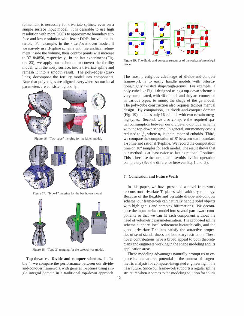
Our experimental results are implemented on a 3 GHzPentium-IV PC with 4 Giga RAM. Our first experimen-tal results (Fig. 16, and Fig. 17) show the applicationof “Two-cube” merging by considering the kitten andbeethoven model as the test datasets. These are the onlymerging types that exist in our component generationframework. For “Type-2,3,4” merging types that do notexist in our framework, we design a special screwdrivermodel and domain to demonstrate the power of “Type-2” merging (Fig. 18). In terms of poly-cube construc-tion, we recognize that “Type-2” merging is very popu-lar to handle the input with long branches. Yet, “Type-

Table 3: Statistics of various test examples:Nc, # of control points;RMS, root-mean-square fitting error (10−3). “bv1”, “bv2”, “ra” and “sd”represent the beethoven (low and high resolution), rockarm, and screw-driver models.

Model Nc RMS Model Nc RMSeight 2058 1.63 wrench 3756 2.3kitten 2840 3.32 g3 2976 1.74bv1 1001 1.8 bv2 3273 1.36ra 4582 3.75 sd 1261 1.65

Table 4: Comparison between our splines and general splines: Spacerequired by fitting; Time to compute derivatives of basis functions; Nc,and Number of cuboids.

ModelOur Method General Method

Space B′ Nc Space B′ Nc

kitten 116802 2.38s 1 300688 4.53s 8eight 24714 2.25s 6 174124 4.35s 15g3 18952 2.17s 16 314832 4.23s 46

3,4” merging cases rarely exist even in the most conven-tional poly-cube domains. Geometrically speaking, theyare more suitable to mimic highly concave shapes. We usethe dark T-junction lines to show control grid knots anduse different colors to represent different merging types.Red/Blue/Yellow marks all “to-be-merged” control pointknots in 3 merging cases, respectively. We also have aclose-up view to show the interior fitting result, demon-strating smoothness around the merging region. The yel-low marks on the control grid highlight the ill-points.

In the second group of experimental results (Fig. 20,Fig 4, Fig. 21, and Fig. 22), we integrate all mergingtypes together to handle the models with high-genus andcomplex bifurcations, including the eight (genus 2), g3(genus 3), rockarm, and wrench (genus 1 with bifurca-tions) model. We first display their component generationresults. Then we show a spline model for one local com-ponent and the final spline results with a close-up view tohighlight the interior fitting and merging regions. Fig. 19also visualizes components’ T-shape/poly-cube structuresin a more efficient way. We use the same color cuboidto represent one component and the edges to show thecuboid connections. Each green box covers cuboids fromthe same T-shape. This structure clearly demonstrates thatonly “Two-cube” and “Type-1” merging are functionallysound in our framework.

In Table 3, we document numbers of control points andfitting error. The T-spline scheme can significantly re-duce the number of control points. The fitting results aremeasured by RMS errors which are normalized to the di-mension of corresponding solid models. Meanwhile, wedemonstrate the interior fitting quality in a close-up viewof each model. Also, the table illustrates that adaptive

11

refinement is necessary for trivariate splines, even on asimple surface input model. It is desirable to use highresolution with more DOFs to approximate boundary sur-face and low resolution with fewer DOFs for volume in-terior. For example, in the kitten/beethoven model, ifwe naively use B-spline scheme with hierarchical refine-ment inside the volume, their control points will increaseto 3718/4850, respectively. In the last experiment (Fig-ure 23), we apply our technique to convert the fertilitymodel, with the noisy surface, into a trivariate spline andremesh it into a smooth result. The poly-edges (gray-lines) decompose the fertility model into components.Note that poly-edges are aligned everywhere so our localparameters are consistent globally.

Figure 16: “Two-cube” merging for the kitten model.

Figure 17: “Type-1” merging for the beethoven model.

Figure 18: “Type-2” merging for the screwdriver model.

Top-down vs. Divide-and-conquer schemes.In Ta-ble 4, we compare the performance between our divide-and-conquer framework with general T-splines using sin-gle integral domain in a traditional top-down approach.

Figure 19: The divide-and-conquer structures of the rockarm/wrench/g3model.

The most prestigious advantage of divide-and-conquerframework is to easily handle models with bifurca-tions/highly twisted shape/high-genus. For example, apoly-cube like Fig. 1 designed using a top-down scheme isvery complicated, with 46 cuboids and they are connectedin various types, to mimic the shape of the g3 model.The poly-cube construction also requires tedious manualdesign. By comparison, its divide-and-conquer domain(Fig. 19) includes only 16 cuboids with two certain merg-ing types. Second, we also compare the required spa-tial consumption between our divide-and-conquer schemewith the top-down scheme. In general, our memory cost isreduced to1

ns, wherens is the number of cuboids. Third,

we compare the computation ofB′ between semi-standardT-spline and rational T-spline. We record the computationtime on 104 samples for each model. The result shows thatour method is at least twice as fast as rational T-splines.This is because the computation avoids division operationcompletely (See the difference between Eq. 1 and 3).

7. Conclusion and Future Work

In this paper, we have presented a novel frameworkto construct trivariate T-splines with arbitrary topology.Because of the flexible and versatile divide-and-conquerscheme, our framework can naturally handle solid objectswith high genus and complex bifurcations. We decom-pose the input surface model into several part-aware com-ponents so that we can fit each component without theneed of volumetric parameterization. The proposed splinescheme supports local refinement hierarchically, and theglobal trivariate T-splines satisfy the attractive proper-ties of semi-standardness and boundary restriction. Thesenovel contributions have a broad appeal to both theoreti-cians and engineers working in the shape modeling and itsapplication areas.

These modeling advantages naturally prompt us to ex-plore its unchartered potential in the context of isogeo-metric analysis for computer-integrated engineering in thenear future. Since our framework supports a regular splinestructure when it comes to the modeling solution for solids

12

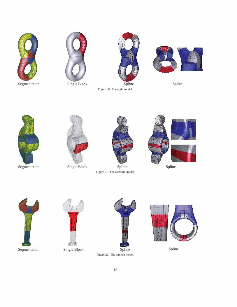
Segmentation Single Block Spline SplineFigure 20: The eight model.

Segmentation Single Block Spline SplineFigure 21: The rockarm model.

Segmentation Single Block Spline Spline

Figure 22: The wrench model.

13

with arbitrary topology, GPU-enabled scientific comput-ing and image-driven shape processing become more de-sirable towards the design of more efficient algorithms.This framework can also be generalized by increasing thedimension of control points to model not only geometrybut also other physical attributes simultaneously.

Figure 23: Mesh smoothing: We convert the fertility model toa trivariatespline and remesh it into a smooth result. Three figures show the compo-nents (with poly-edges), the globally aligned parameters,the remshingresult (with interior cut views), respectively.

References

[1] K. Wang, X. Li, B. Li, H. Xu, H. Qin, Restricted trivariatepoly-cube splines for volumetric data modeling, IEEE Transactions onVisualization and Computer Graphics (2011) to appear.

[2] T. Sederberg, D. Cardon, G. Finnigan, N. North, J. Zheng,T. Ly-che, T-spline simplification and local refinement, ACM Transac-tions on Graphics 23 (3) (2004) 276–283.

[3] B. Li, X. Li, K. Wang, H. Qin, Generalized polycube splines, in:SMI10:International Conference on Shape Modeling and Applica-tions, 2010, pp. 261–266.

[4] A. Myles, Y. Yeo, J. Peters, Gpu conversion of quad meshestosmooth surfaces, in: SPM’08:Proceedings of the 2008 ACM sym-posium on Solid and Physical Modeling, 2008, pp. 321–326.

[5] W. Song, X. Yang, Free-form deformation with weighted t-spline,The Visual Computer 21 (3) (2005) 139–151.

[6] T. Hughes, J. Cottrell, Y. Bazilev, Isogeometric analysis: Cad, fi-nite elements, nurbs, exact geometry adn mesh refinement, Com-puter Methods in Applied Mechanics and Engineering 194 (2005)4135–4195.

[7] C. Rossl, F. Zeilfelder, G. Nurnberger, H. Seidel, Reconstructionof volume data with quadratic super splines, IEEE Transactions onVisualization and Computer Graphics 10 (4) (2003) 397 – 409.

[8] W. Li, N. Ray, B. Levy, Automatic and interactive mesh tot-splineconversion, in: Symposium on Geometry Processing, 2006, pp.191–200.

[9] H. Wang, Y. He, X. Li, X. Gu, H. Qin, Polycube splines, ComputerAided Design 40 (6) (2008) 721–733.

[10] X. Zhou, J. Lu, Nurbs-based galerkin method and application toskeletal muscle modeling, in: ACM Solid and Physical ModelingSymposium, 2005, pp. 71–78.

[11] T. Martin, E. Cohen, R. Kirby, Volumetric parameterization andtrivariate b-spline fitting using harmonic functions, ComputerAided Geometric Design 26 (6) (2009) 648–664.

[12] Y. Zhang, Y. Bazilevs, S. Goswami, C. L. Bajaj, T. Hughes,Patient-specific vascular nurbs modeling for isogeometricanaly-sis of blood flow, Computer Methods in Applied Mechanics andEngineering 196 (29-30) (2007) 2943 – 2959.

[13] T. Martin, E. Cohen, Volumetric parameterizations of complexobjects by respecting multiple materials, Computer and Graphics34 (3) (2010) 187–197.

[14] T. Sederberg, J. Zheng, A. Bakenov, A. Nasri, T-splinesand t-nurccs, ACM Transactions on Graphics 22 (3) (2003) 477–484.

[15] T. Sederberg, J. Zheng, D. Sewell, M. Sabin, Non-uniform recur-sive subdivision surfaces, in: SIGGRAPH98, 1998, pp. 387–394.

[16] H. Ipson, T-spline merging, Master’s thesis, Brigham Yong Uni-versity (2005).

[17] T. Sederberg, G. Finnigan, X. Li, H. Lin, H. Ipson, Watertighttrimmed nurbs., ACM Transactions on Graphics 27 (3) (2008) 1–8.

[18] A. Myles, N. Pietroni, D. Kovacs, D. Zorin., Feature-aligned t-meshes, ACM Transactions on Graphics 29 (4) (2010) 117:1–117:11.

[19] C. Loop, S. Schaefer, G2 tensor product splines over extraordinaryvertices, in: Proceedings of the Symposium on Geometry Process-ing, SGP ’08, 2008, pp. 1373–1382.

[20] J. Peters, J. Fan, The projective linear transition mapfor construct-ing smooth surfaces, in: Proceedings of the 2010 Shape ModelingInternational Conference, SMI ’10, 2010, pp. 124–130.

[21] M. Tarini, K. Hormann, P. Cignoni, C. Montani, Polycubemaps,ACM Transactions on Graphics 23 (3) (2004) 853–860.

[22] J. Lin, X. Jin, Z. Fan, C. Wang, Automatic polycube-maps, in:Geometric Modeling and Processing, 2008, pp. 3–16.

[23] J. Gregson, A. Sheffer, E. Zhang, All-hex mesh generation via vol-umetric polycube deformation, Computer Graphics Forum 30 (5)(2011) 1407–1416.

[24] P. Alliez, D. Cohen-Steiner, M. Yvinec, M. Desbrun, Variationaltetrahedral meshing, ACM Transactions on Graphics 24 (2005)617–625.

[25] D. Yan, W. Wang, B. Levy, Y. Liu, Efficient computation of clippedvoronoi diagram, Computer Aided DesignTo appear.

[26] Y. Wang, X. Gu, T. Chan, P. Thompson, S. Yau, Volumetric har-monic brain mapping, in: IEEE Symposium on Biomedical Imag-ing:macro to nano, 2004, pp. 1275–1278.

[27] J. Xia, Y. He, X. Yin, S. Huan, X. Gu, Direct-product volumet-ric parametrization of handlebodies via harmonic fields, in: ShapeModeling International Conference, 2010, pp. 3–12.

[28] R. Liu, H. Zhang, A. Shamir, D. Cohen-Or, A part-aware surfacemetric for shape analysis, Computer Graphics Forum (Special Is-sue of Eurographics 2009) 28 (2) (2009) 397–406.

[29] L. Shapira, A. Shamir, D. Cohen-Or, Consistent mesh partitioningand skeletonisation using the shape diameter function, TheVisualComputer 24 (2008) 249–259.

[30] T. Dey, K. Li, J. Sun, On computing handle and tunnel loops, in:International Conference on Cyber Worlds, 2007, pp. 357–366.

[31] X. Li, X. Gu, H. Qin, Surface mapping using consistent pants de-composition, IEEE Transactions on Visualization and ComputerGraphics 15 (4) (2009) 558–571.

[32] G. Taubin, A signal processing approach to fair surfacedesign, in:SIGGRAPH ’95: Proceedings of the 22nd Annual Conference onComputer graphics and interactive techniques, 1995, pp. 351–358.

[33] M. Floater, Mean value coordinates, Computer Aided GeometricDesign 20 (1) (2003) 19–27.

[34] K. Zhou, J. Huang, J. Snyder, X. Liu, H. Bao, B. Guo, H.-Y.Shum, Large mesh deformation using the volumetric graph lapla-cian, ACM Transactions on Graphics 24 (3) (2005) 496–503.

14