Embed Size (px)
Citation preview

Electronic Journal of Statistics
Vol. 2 (2008) 605–633ISSN: 1935-7524DOI: 10.1214/08-EJS200
On the asymptotic properties of the
group lasso estimator for linear models
Yuval Nardi∗ and Alessandro Rinaldo†
Department of StatisticsCarnegie Mellon University
Pittsburgh, PA 15213-3890 USAe-mail: [email protected]; [email protected]
Abstract: We establish estimation and model selection consistency, pre-diction and estimation bounds and persistence for the group-lasso estimatorand model selector proposed by Yuan and Lin (2006) for least squares prob-lems when the covariates have a natural grouping structure. We considerthe case of a fixed-dimensional parameter space with increasing sample sizeand the double asymptotic scenario where the model complexity changeswith the sample size.
AMS 2000 subject classifications: Primary 62J05; secondary 62F12.Keywords and phrases: Least Squares, Sparsity, Group-Lasso, ModelSelection, Oracle Inequalities, Persistence.
Received March 2008.
1. Introduction
In recent years there has been a rapidly growing interest in penalized leastsquares problems via ℓ1 regularization, especially in high dimensional settingswhere the model complexity is comparable or even larger than the sample size.The lasso, originally put forward by Tibshirani (1996) for linear regressionmodels, is a regularization procedure in which the penalty for model complexityis the ℓ1 norm of the estimated coefficients. It has the crucial advantages of be-ing a convex problem, thus computationally feasible even when the numberof predictor is larger than the sample size, and of producing solutions that aresparse, i.e. containing zero components. These two key properties make thelasso simultaneously a shrinkage estimation and a model selection procedurethat is viable in high-dimensional problems where traditional model selectioncriteria are not feasible. Furthermore, the lasso has been shown to have optimaltheoretical properties: model selection, or sign consistency, or sparsistency (see,e.g., Meinshausen and Buhlmann, 2006; Wainwright, 2006, 2007; Zhao and Yu,2006), consistency and oracle properties (see, e.g. Meinshausen and Yu, 2006;Bickel et al., 2007; Bunea et al., 2007a,b; Zhang, 2007; Koltchinskii, 2005;Zhang and Huang, 2007), and persistence (Greenshtein and Ritov, 2006;Greenshtein, 2006).
∗Supported in part by NSF grant EIA–0131884 and Army contract DAAD19-02-1-3-0389.†Supported in part by NSF grant DMS-0631589 and a grant from the Pennsylvania De-
partment of Health through the Commonwealth Universal Research Enhancement Program.
605

Y. Nardi and A. Rinaldo/The log-linear group lasso estimator 606
Researches have also devised few extensions of the lasso that are suited todeal with regression problems in which the explanatory variables are groupedor are organized in a hierarchal manner and, at the same time, exhibit similarcomputational ease and the shrinkage properties of the lasso. We mention, inparticular, the group-lasso procedure by Yuan and Lin (2006) and its extensionby Kim et al. (2006), the elastic net regularization by Zou and Hastie (2005),the hierarchical lasso by Zhou and Zhu (2007), regularization methods basedon ℓ∞ penalty by Gilbert et al. (2005) and the very general CAP penalties byZhao et al. (2007). Most of these procedures essentially comprise a penalty forthe model complexity that results from a composition of the ℓ1 norm with someother norm computed over each group of parameters, thus exhibiting a behaviorthat, at the group level, resembles that of the lasso solution. Besides ANOVAmodels, the group-lasso penalty has been applied to generalized linear models inDahinden et al. (2006), Meier et al. (2006) and Nardi and Rinaldo (2007) andto non-parametric problems in Bach (2007) and Ravikumar et al. (2007).
The general purpose of this paper is to prove for the group-lasso estimator de-scribed in Yuan and Lin (2006) the same type of optimality properties that havebeen established for the lasso estimator. In particular, we will derive conditionsensuring estimation and model selection consistency, prediction and estimationconsistency, oracle properties and persistence. For the case of a fixed-dimensionalparameter space, Bach (2007) derives some conditions for estimation and modelselection consistency. For the double-asymptotic scenario in which the dimen-sion of the parameter space grows with the sample size, a rigorous study of theperformance of the group-lasso seems to be missing in the statistical literature.Our contributions include novel consistency and asymptotic normality resultsfor the fixed-dimensional parameter space, model selection consistency when thenumber of predictors is larger than the sample size, oracle inequalities and per-sistence properties. Our methods of proofs are based on non-trivial extensionsand generalizations of condition and results for the lasso procedure already inexistence in the literature.
The paper is organized as follows. Section 2 introduces the group-lasso set-tings for least square problems. In section 3 we establish estimation and modelselection consistency and asymptotic normality under the traditional scenarioof increasing sample size and fixed parameter space. The conditions we imposeare of different nature than the ones introduced in Bach (2007) and the resultswe obtain complement that analysis. In section 4 we investigate the propertiesof the group-lasso solution under the more complex, double-asymptotic scenarioin which both the sample size and the model complexity grow simultaneously.In section 4.1 we provide a sufficient condition guaranteeing uniqueness of thegroup-lasso solution when the number of covariates is larger than the samplesize. In section 4.2 we provide conditions for model selection consistency thatholds even when the number of covariates grow at a larger rate than the samplesize and in section 4.3 we derive finite sample bounds that can be used to estab-lish consistency for estimation and prediction. Finally, in section 4.4 we derivetwo persistence properties. All the proofs are gathered in section 5 and in theAppendix.

Y. Nardi and A. Rinaldo/The log-linear group lasso estimator 607
2. The group-Lasso settings
Let H be an index set representing a class of linear subspaces of Rn, each
subspace being spanned by the columns of a n× dh matrix Xh, where h rangesover H. We will be assuming henceforth that the set H is known and has beenassigned a total ordering, and we will always be using such an ordering. LetX be a n × d design matrix formed by concatenating the design matrices Xh,h ∈ H, with d =
∑h dh. While we allow for non-zero correlations among groups,
namely X⊤h Xh′ 6= 0 for h 6= h′, we will be making the simplifying assumption
1
nX⊤
h Xh = Idh, ∀h ∈ H,
where Idhdenote the dh-dimensional identity matrix, a condition that can be
enforced via the Gram-Schmidt orthogonalization procedure.For a subset H′ ⊂ H, we will write (H′)c = H\H′ and, if x ∈ R
d, we will usethe notation xH′ = vec{xh, h ∈ H′} for the d′-dimensional subvector comprisedby the blocks of x indexed by H′, where d′ =
∑h∈H′ dh. Similarly, if H1 and
H2 are two subsets of H, and M a d× d matrix, we will write
MH1,H2
for the (∑
h∈H1dh) × (
∑h∈H2
dh) block matrix, with blocks indexed by thesubsets H1 and H2. In particular, if H1 = H2, we will simply write MH1 .
We assume that the n-dimensional observed vector Y satisfies the linearmodel
Y = Xβ0 + ǫ, (1)
where ǫ is a n-dimensional vector of iid errors, with distributional properties tobe specified below, and β0 is the unknown d-dimensional vector of true coeffi-cients. Then, the vector β0 can be represented as vec{β0
h, h ∈ H}, the concate-nation of |H| vectors, where β0
h ∈ Rdh , for each h ∈ H. Our crucial modeling
assumption is that some of the subvectors of β0 are zero and we will denote byH0 = {h : β0
h 6= 0} the unknown index set of non-zero subvectors of β0. Then,the true model complexity is given by d0 =
∑h∈H0
dh < d.
We consider the problem of estimating both β0 and H0 in the non-trivialsituation in which the cardinality |H0| of the number or subspaces spanning thetrue mean vector of the response variable Y is smaller than the total number |H|of candidate subspaces. In essence, the estimation of the true underlying modelH0 requires identifying, based on Y , the zero subvectors of β0 and removing theblocks indexed by Hc
0. This may be naturally formulated as a penalized leastsquare problem with a ℓ0 penalty on the cardinality of the subspaces included.Effectively, this entails considering all possible subsets of H, an NP-hard taskthat is computationally infeasible, when |H| (and therefore d) is large. Instead,Yuan and Lin (2006) propose to use the group-lasso penalty, which is a convexrelaxation to the ℓ0 penalty based on the combination of the ℓ1 penalty over thenumber of subspaces with the ℓ2 penalty on the estimated coefficients of each

Y. Nardi and A. Rinaldo/The log-linear group lasso estimator 608
subspace. The resulting group-lasso estimator is obtained as the solution to theconvex problem
infβ∈Rd
1
2n‖Y − Xβ‖2
2 + λ∑
h
λh‖βh‖2, (2)
where λ and {λh, h ∈ H}, are tuning parameters that depend on the samplesize n. A reasonable choice for λh is
√dh, so that larger subspaces are penalized
more heavily. The group-lasso regularization is an extension of the lasso, orℓ1 penalty function, and consists of applying first the ℓ2 penalty to individualblocks, to promote non-sparsity, and then the ℓ1 norm to the resulting blocknorms, to promote block sparsity. Notice also that the group-lasso problem (2)includes as a special case the lasso and adaptive lasso (see Zou, 2006) problemin which |H| = d and each h correspond to the 1-dimensional subspace of R
n
spanned by the corresponding column of the design matrix X.Equation (2) is the Lagrangian function (with Lagrangian multipliers {λλh, h ∈
H}) of the equivalent convex problem
infβ∈Rd
1
2n‖Y − Xβ‖2
2
s.t. ‖βh‖2 ≤ th,
(3)
where {th, h ∈ H} are non-negative constants. In fact, there exists a correspon-dence between the coefficients {th, h ∈ H} and {λλh, h ∈ H} of (3) and (2),respectively. In this article, we will mostly focus on the more popular, uncon-strained formulation (2), which has, in particular, the advantage of letting onechoose in a more direct way the regularization parameters. The constrained set-tings (3) will be used in Section 4.4 to establish persistence properties of thegroup-lasso.
In our analysis, we will study the asymptotic properties of the group-lassoestimator β, defined as a minimizer of (2), and of the associated group-lassomodel selector
H = {h : βh 6= 0}. (4)
We will consider two asymptotic regimes. In the simpler, traditional scenario,we assume that the model complexity is fixed and that only the sample size nincreases. In the second, more modern, scenario, the model complexity increaseswith the sample size and we will then study the group-lasso solutions to asequence of linear models in which |H| and {dh, h ∈ H} grow with n. In fact, weallow for d to grow at a faster rate than n. For ease of readability, we will notmake the dependence of H, {dh, h ∈ H}, λ, X, ǫ and {λh, h ∈ H} on n explicit,although it will be apparent that all those quantities may change with n.
We conclude this section with some computational remarks. The subgradientconditions for the problem (2) are
− 1
nX⊤
h
(Y − Xβ
)+ λλh
βh
‖βh‖2
= 0 if βh 6= 0
− 1
nX⊤
h
(Y − Xβ
)+ λλhzh = 0 if βh = 0,
(5)

Y. Nardi and A. Rinaldo/The log-linear group lasso estimator 609
where zh are generic vectors such that ‖zh‖2 ≤ 1 for all h. Because the objectivefunction in (2) is convex on R
d, the first-order conditions obtained by solvingthe sub-gradient equations produce the solutions to the group-lasso problem.By inspecting the sub-gradient conditions (5), Yuan and Lin (2006) devise amodification of the LARS algorithm by Efron et al. (2004) to account for theblock structure of the penalty function that can be used to solve (2) numerically.Dahinden et al. (2006) improve on this method and develop a different compu-tational strategy based on a block-coordinate gradient descent method in thecontext of logistic regression, which can be adapted to the present settings. SeeDahinden et al. (2006) and, in particular, Zhao et al. (2007) for further detailsand some discussion on the computational aspects of the group-lasso estimatorand on the choice of the regularization parameters.
2.1. Example: ANOVA models
Consider an ANOVA design, arising from the cross-classification of K categoricalvariables, each taking value on a finite set Ik = {1, . . . , Ik}, for k = 1, . . . , K.Let I =
⊗k Ik be the set of cells and I =
∏k Ik the total number of cells.
Also, for each i ∈ I, let ni be the total number of observations in cell i. ThenH = 2K, the power set of K = {1, . . . , K}. Each h ∈ H0 represents an effect.For example, h = ∅ corresponds to the grand mean, a subset h with |h| = 1 toa main effect and, more generally, a subset h to an interaction effect among thevariables indexed by h. The true model can be represented as H0 ⊆ 2K.
As h ranges over H, RI can be decomposed into the direct sum of orthogonal
subspaces indexed by h, each with dimension∏
j∈h(Ij − 1) (see, e.g. Rinaldo,2006). Let Uh be a matrix of full column rank spanning the subspace index byh ⊂ K. Then, the columns of
⊕h∈2K Uh form a basis for R
I. Next, let T be an × I matrix of the form
11 0 . . . 00 12 . . . 00 0 . . . 1I
,
where each 1i is a ni-dimensional vector of ones, and Xh = TUh. Notice thatdim(range(Uh)) = dim(range(Xh)), provided each cell is positive. Then, then × I matrix
X =⊕
h∈2K
Xh
has full column rank and its columns span a I-dimensional subspace in Rn.
Notice that, for any h 6= h′ ∈ 2K, while U⊤h Uh′ = 0, it is no longer the case that
X⊤h Xh′ = 0 when the cells ni differ, i.e. when the model is unbalanced or when
some cells are empty. It is clear that the group-lasso settings described aboveinclude as special cases unbalanced and empty-cells ANOVA models, for whichthe usual decomposition of sums of square does not hold.

Y. Nardi and A. Rinaldo/The log-linear group lasso estimator 610
3. Fixed-d asymptotics
In this section we derive conditions for model selection and estimation con-sistency when the sample size n increases, while the parameter space remainsfixed. Our consistency results rely on different assumptions and slightly differentsettings than the analogous results in Bach (2007), and our analysis providesnovel insights into this problem. Furthermore, we obtain rates of consistencyand asymptotic normality.
We will use the classical assumptions for consistency of the ordinary leastsquares solutions:
(F1) limn→∞1nX⊤X → M, with M positive definite;
(F2) the errors ǫi are iid with mean zero and finite second moment σ2.
To motivate our analysis, we first consider the necessary conditions for thegroup-lasso procedure to be model selection consistent, namely
P{H = H0
}→ 1, as n → ∞, (6)
where H is defined in (4). An adaptation of Theorem 3 in Bach (2007) yieldsthat, under assumption (F1) and (F2), (6) holds only if the weakly irreducibilitycondition
maxh′∈Hc
0
1
λh′
∥∥Mh′,H0M−1H0
BH0βH0
∥∥2≤ 1, (7)
is verified, where BH0 denotes the d0-dimensional block-diagonal matrix withblocks {
Idh
λh
‖βh‖2, h ∈ H0
}.
We remark that (7) generalizes an analogous necessary condition for model selec-tion consistency of the lasso (see Zou, 2006; Zhao and Yu, 2006; Yuan and Lin,2006). Below, we derive a different necessary condition for model selection con-sistency, which provides a rationale for the results we derive in the remainderof this section.
Proposition 3.1. Under assumption (F1) and (F2), the model selection con-sistency property (6) holds only if
√nλλh → ∞, ∀h 6∈ H0.
Using the previous condition, it seems natural to consider sequences of penalty
parameters such that λλh = O(
1√n
)if h ∈ H0, and
√nλλh → ∞ otherwise,
which will also satisfy the weakly irreducibility condition (7). Implicitly, thisidea is behind both Theorem 3.2 and 3.3.
The weak irreducibility condition and the other necessary condition of Propo-sition 3.1 both have the undesirable feature of depending on the unknown indexset H0 of non-zero blocks. To remedy this problem, in the following result wedescribe an oracle procedure which automatically yields model selection consis-tency without knowing H0. This estimator is obtained as a direct generalization

Y. Nardi and A. Rinaldo/The log-linear group lasso estimator 611
to the group-lasso framework of the adaptive lasso penalty put forward by Zou
(2006). We let βOLS =(X⊤X
)−1X⊤Y for the least squares estimate of β. In the
proof we essentially follow Zou (2006) and Knight and Fu (2000) and generalizetheir results to our settings.
Theorem 3.2. Assume (F1) and (F2) and let λh = 1
‖βOLSh
‖γ
2
, for some γ > 0
such that n(γ+1)/2λ → ∞. If√
nλ → 0, the model selection consistency property(6) is satisfied and, furthermore,
√n(β − β0)
d→ Z, (8)
where ZH0 ∼ Nd0 (0, σ2M−1H0
) and ZHc0
= 0.
Remark. The only property of the ordinary least squares estimate βOLS thatwas used in the proof is its
√n-consistency. This is enough to guarantee that
the penalty parameters {λh, h ∈ Hc0} corresponding to the index set of the
zero subvectors of β0 are very large, with high probability for all n big enough.More generally, the Theorem remains true also when βOLS is replaced by anyan-consistent estimator, where an → ∞, provided aγ
n
√nλ → ∞.
We conclude this section with one final consistency result for the group-lassoestimator, which demands the knowledge of H0. Unlike the consistency resultsderived in (Bach, 2007, Section 2), the weakly irreducibility condition (7) isreplaced by conditions on the asymptotic behavior of
√nλλh, h ∈ H. Despite
its reduced practical value, this result has the merit of showing explicitly thatthe penalty terms for the zero and non-zero blocks need to have a differentasymptotic behavior.
Theorem 3.3. Assume (F1), (F2) and further assume that the (possibly ran-
dom) sequence {an}, with an = |H0|maxh∈H0 λh, satisfy λanp→ 0 as n → ∞.
Then ‖β − β0‖2 = OP
(1√n
+ λan
). Furthermore, if λan = OP
(1√n
)and
√nλλh
p→ ∞ for each h 6∈ H0, then the conclusions of Theorem 3.2 still hold.
Remark. The previous Theorem covers cases in which estimation consistencymay hold (at a suboptimal rate) but not model selection consistency.
Theorem 3.2 and Theorem 3.3 both establish that the group-lasso estimatoris asymptotically optimal, namely unbiased and efficient, and, therefore, offersthe same asymptotic guarantees as the ordinary, unpenalized, least squares es-timator. However, unlike the ordinary least squares, the group-lasso solutionscomes equipped with a built-in penalty for sparsity, so that some of its blockscomponents will be zero. In fact, and this is key, as n increases, these zero com-ponents will be the same zero components of the true vector of coefficients β0,with probability tending to 1. In contrast, the solutions to the ordinary leastsquares are all non-zero, thus making it much less effective at recovering H0.
Y. Nardi and A. Rinaldo/The log-linear group lasso estimator 612
4. Double asymptotics
We turn now to the study of double-asymptotic scenario in which |H| → ∞ andthe block-dimensions {dh, h ∈ H} are allowed to change with n. In particular,this includes situations in which d >> n, i.e. d grows faster than n.
To simplify our derivations, we will enforce a normality assumption on thevector ǫ of errors:
(N) ǫi ∼ N(0, σ2), 1 ≤ i ≤ n.
Specific cases in which this assumption can be relaxed are discussed as we pro-ceed with our analysis.
4.1. Uniqueness of the group-Lasso solution
When d > n, there is a (d−n) dimensional affine space of vectors satisfying themodel equation (1). As a result, the solution to (2) needs not be unique and,therefore, it may no longer make sense to refer to “the” group-lasso estimator ormodel selector. To overcome this problem, we may want to impose the followingcondition, which is enough to guarantee uniqueness of the model representation(1) and, therefore, of the group-lasso solution:
(U(c)) maxh′ 6=h ‖X⊤h′Xh‖2 ≤ λh′λh
(1+2c)δ|H0| , for some constants c > 0 and δ > λ2max,
where, for a m × p matrix A, ‖A‖2 denotes the operator norm with respectto the Euclidian metric. In stating the assumption, we make explicit only thedependence on the more relevant constant c.
Proposition 4.1. Under assumption (U(c)), if β1 and β2 satisfy (1) with|{h : βi
h 6= 0}| ≤ |H0|, for i = 1, 2, then β1 = β2.
Remarks.
1. Assumption (U(c)) is the group-lasso equivalent of Assumption 2 in Lounici(2008) on the maximal mutual coherence between different columns of thedesign matrix X, which is
maxi 6=j
1
n|Mi,j| ≤
1
ρ(1 + 2c)d0,
where ρ > 1 and c > 0. We point out that uniqueness of the represen-tation (1) follows also from this mutual coherence condition. However,assumption (U(c)) is more naturally tailored to the problem at hand and,furthermore, implies the important (RE(|H0|, c)) condition (see Propo-sition 4.4 below), which is essential to establish the bounds derived inSection 4.3.
2. Alternatively, one may consider investigating conditions guaranteeing unique-ness of the group-lasso solution (2) directly, rather of the model represen-tation, following the arguments used in Osborne et al. (2000) for the lasso
Y. Nardi and A. Rinaldo/The log-linear group lasso estimator 613
problem. Although it is apparent from their analysis that |H| ≤ n, i.e.the number of non-zero blocks is no larger than the sample size, extend-ing the polyhedral arguments of Osborne et al. (2000, Section 3.1) to thegroup-lasso penalty appears problematic.
4.2. Sparsistency
In this section, we provide conditions for the model selection consistency (6),or sparsistency, of the group-lasso model selector under the double asymptoticsettings.
To this end, let O be the event that there exists a solution β to (2) such that
‖βh‖2 > 0 for all h ∈ H0, and βh = 0 for all h ∈ Hc0. Then, the sparsistency
property isP(O) → 1, n → ∞. (9)
We will make the following assumptions:
(S1) the smallest eigenvalue of 1n
(X⊤
H0XH0
)is bounded below by a constant
Cmin > 0;(S2) letting α = minh∈H0 ‖β0
h‖∞,
1
α
[√logd0
n+√
d0λ maxh∈H0
λh
]→ 0;
(S3) for some 0 < ǫ < 1 and every h ∈ Hc0,
∥∥∥X⊤h XH0
(X⊤
H0XH0
)−1∥∥∥
2≤ 1 − ǫ√∑
h∈H0λ2
h
;
(S4)
1
λ
√log(d − d0)
nmaxh∈Hc
0
√dh
λh→ 0.
Theorem 4.2. Under the assumptions (N) and (S1)-(S4), the sparsistencyproperty (9) holds.
Remarks. The conditions of Theorem 4.2 deserve a few comments.
1. From the proof, it can be seen that we can combine (S1) and (S2) intoone assumption
1
α
[√logd0
nCmin+√
d0λ maxh∈H0
λh
]→ 0,
thus allowing the minimal eigenvalue of 1n
(X⊤
H0XH0
)to vanish at a rate
slower than 1α2
log d0
n .

Y. Nardi and A. Rinaldo/The log-linear group lasso estimator 614
2. The normality assumption (N) is by no means crucial. In fact, it is enoughto require the errors to be independent, sub-gaussian random variables,with second moments bounded uniformly in n. Then, by applying, forexample, Lemma 2.3 in Massart (2007), the conclusions of the Theoremwould hold unchanged.
3. If λh =√
dh then conditions (S4) simplifies to
log(d − d0)
nλ2→ 0.
which is the same rate appearing in Equation 15 b) in Wainwright (2006)for the simpler lasso penalty.
4. It is apparent from condition (S4) that not only can d be much bigger thenn, but it can in fact grow at at faster rate than n. In particular, condition(S4) formalizes quite explicitly the notion that the true model should besparse in order for the group-lasso model selector to be successful.
5. Because the group-lasso solution may not be unique, Theorem 4.2 onlyimplies the existence of a sequence of solutions guaranteeing sparsistency.In order to obtain a more satisfactory result, one may want to enforce alsothe uniqueness condition (U(c)), for some c > 0.
4.3. Inequalities for prediction and estimation
We now derive oracle inequalities for the prediction and estimation loss of thegroup-lasso estimator.
As a main technical step in our derivations (which generalizes standard ar-guments found, for example, in Bunea et al., 2007a,b; Bickel et al., 2007), theprediction and estimation bounds we establish hold on the event
A =⋂
h
{2√n
∥∥X⊤h ǫ∥∥
2<
√nλλh
}.
Therefore, we must impose conditions implying that A occurs with probabilitytending to 1, as both n and the model complexity increase. To that end, weformulate the asymptotic condition
(A) minh{ nσ2 λ2λ2
h − dh} − log |H| → ∞,
which will guarantee that the inequalities given below are meaningful for nlarge enough and also offers some characterizations of the rates of growth of theregularization parameters.
Lemma 4.3. Assume (N) and (A). Then, P(A) → 1, as n → ∞.
Remarks.
1. Assumption (A) provides general guidelines for choosing the tuning pa-rameters λ and {λh, h ∈ H}. In particular, if λh =
√dh for each h, the
condition reduces to
dminn
σ2λ2 − log |H| → ∞,

Y. Nardi and A. Rinaldo/The log-linear group lasso estimator 615
where dmin = minh dh. For such a choice of λh, for example, we can use
λ = σ√
Cn
n, where Cn is such that
Cndmin
log |H| → ∞.
Since dmin ≥ 1, we can set
λ = Aσ
√log |H|
n,
for some A > 1.2. Alternatively, and in less generality, if again λh =
√dh for each h, we
could consider the event
A′ =
d⋂
i=1
{2
n
∣∣X⊤i ǫ∣∣ < λ
}.
where Xi denotes the i-th column of the matrix X. Then, for
λ = Aσ
√logd
n
with A ≥ 2, a standard Gaussian tail bound (see, e.g., van de Geer, 2007,Lemma 3.8) yields
1 − P(A′) ≤ 2 exp
{−A2
8log d
},
which vanishes provided d → ∞. Notice that this case is covered by as-sumption (A). Then, using the event A′ and Cauchy-Schwarz’s inequalityin equation (39) in the proof of Theorem 4.6, it is easy to see that theresults of this section would hold with A replaced by A′.
3. It appears that the Gaussianity assumption (N) is quite important in thiscontext, as it is used in a fundamental way to establish condition (A). If,instead of the event A, one considers the event A′ (with the additionalconstraints λh =
√dh for each h), then Gaussianity is not necessary and,
with λ = σ
√(log d)(1+η)
n for some η > 0, one can still guarantee a vanishing
probability for A′ under the slightly stronger requirement (log d)(1+δ) =o(n) and some additional mild constraints. See Lounici (2008, Theorem 3)for a formal argument.
Another key assumption to our results is given below, where s is an integerand c a positive number:
(RE(s, c))
minH′⊆H : |H′|≤s
minβ∈Rd : γ=Λβ,
∑h∈(H′)c
‖γh‖2≤c∑
h∈H′‖γh‖2
‖Xβ‖2√n‖βH′‖2
≡ κ(h, c) > 0.
Y. Nardi and A. Rinaldo/The log-linear group lasso estimator 616
Here Λ is the d×d matrix with diagonal vec{1dhλh, h ∈ H} and 1dh
denotes thedh-dimensional vector with entries all equal to 1. This assumption specializes therestricted eigenvalue assumption introduced by Bickel et al. (2007) to analyzethe L2 consistency property of the lasso procedure.
In particular, in the special case in which s = |H0|, the (RE(s, c)) assumptionis implied by the uniqueness assumption (U(c)), as demonstrated in the nextproposition.
Proposition 4.4. Let U(c, δ) be satisfied. Then, assumption RE(|H0|, c) holds.
Our first result provides finite sample bounds for the prediction and estima-tion loss and for the number of non-zero blocks of the group-lasso estimatorunder the linear model (1), with unknown block-support set H0.
Theorem 4.5. Assume (N) and (RE(|H0|, 3)). On the event A,
‖β − β0‖2 ≤ 16λ
κ20λmin
|H0|, (10)
where λmin = minh λh,
1
n‖X(β − β0)‖2
2 ≤ 16λ2|H0|κ2
0
, (11)
and
|H| ≤ 64Cmax|H0|κ2
0λ2min
, (12)
where Cmax is the largest eigenvalue of 1n
(X⊤
H0XH0
)and κ0 = κ(|H0|, 3).
Next, we establish a more general oracle inequality for the prediction loss ofthe group-lasso estimator which covers the case of a mispecified model. Specifi-cally, rather than assuming that the true model is linear, we consider the moregeneral model
Y = f0(X) + ǫ,
for some unknown, possibly non-linear, function f0 of the covariates.
Theorem 4.6. Under the assumptions (N) and RE(s, 3+4/ǫ), on the event A,
1
n‖Xβ − f0(X)‖2
2
≤ infβ : |H(β)|≤s
{(1 + ǫ)
1
n‖Xβ − f0(X)‖2
2 +4
κ2
(4
ǫ+ ǫ + 4
)λ2|H(β)|
}, (13)
where H(β) = {h : βh 6= 0} and κ = κ(s, 3 + 4/ǫ).
Remarks.
1. Recall that, under our assumption (A), the event Ac has vanishing prob-ability, so the bounds we obtain holds with large probability, for n bigenough.

Y. Nardi and A. Rinaldo/The log-linear group lasso estimator 617
2. In both Theorems (4.6) and (13), we do not enforce the uniqueness condi-tion (U(c)), and, therefore, the conclusions hold for any solution to (2). Infact, because of Proposition 4.4, we can replace the RE(s, c) conditions inboth Theorems (4.6) and (13) by the appropriate U(c) conditions, whichwould guarantee the same results and also uniqueness of the group-lassoestimator.
3. The inequalities derived above directly generalize the corresponding boundsestablished by Bunea et al. (2007a) and Bickel et al. (2007) for the lassoproblem.
4. From both Theorems, it is possible to get rates of prediction and estima-tion consistency of the group-lasso. These rates depend crucially on thechoice of the tuning parameters compatible with assumption (A), in par-ticular of λ. See Remark 1. after Lemma 4.3 for some comments on the
possible values for λ. In particular, for λh =√
dh and λ = Aσ√
log |H|n
,
for some A > 1, we obtain rates that are comparable to lasso rates, withthe number of parameters replaced by the number of blocks. This is dueto the nature of our assumption (RE(s, c)).
4.4. Persistence
In this final section, we change our settings and adopt the double-asymptoticframework of Greenshtein and Ritov (2006) and Greenshtein (2006). Our goalis to study the risk consistency of the group-lasso solutions under a triangulararray framework for the random vector Q = (Y, X), where Y is the responsevariable and X = (X1, . . . , Xd) the vector of covariates. We are concerned withthe predictive risk R(β) = E(Y − Xβ)2 , where the expectation is with respectto the joint distribution P(X,Y ) of Y and X.
Specifically, let βn be an estimator based on an iid sample (Q1, . . . , Qn) of size
n from P(X,Y ) and let R(β) = E(Y − βX|Q1, . . . , Qn), for a new iid observation(Y, X) ∼ P(Y,X). Just like above, we allow d to grow unbounded with n. Let{Sn} be a sequence of sets of increasing dimensions. A sequence of estimators
{βn} is said to be persistent with respect to {Sn} if
R(βn) − infβ∈Sn
R(β)p→ 0, n → ∞.
Notice that, in order for persistence to hold, it is not necessary for the bestpredictor of Y based on X to be linear.
We assume that the random covariates X have a grouping structure, which werepresent using the same notation and conventions of Section 2. Accordingly, weconsider the following two sequences of sets, each of them providing a differentform of group penalty:
Bn =
{β :∑
h
√dh‖βh‖2 ≤ bn
}

Y. Nardi and A. Rinaldo/The log-linear group lasso estimator 618
andCn =
{β : |{h, βh 6= 0}| ≤ cn
},
for some sequences of numbers {bn} and {cn} to be determined.Letting γ = (−1, β1, . . . , βp), we can write R(β) = γ⊤Σγ, where Σ = EQQ⊤.
The empirical equivalent of this quantity is R(β) = γ⊤Σγ, where
Σ =1
n
∑
i
Qi(Qi)⊤.
In these new settings, the group-lasso estimator β with respect to the se-quence {Sn} of sets of potential coefficients, which can be {Bn} or {Cn}, iscomputed as
β = minβ∈Sn
R(β). (14)
Following Zhou et al. (2007), we impose the conditions
(P1) E|Zjk|q ≤ q!Aq−2B/2, for each j, k = 1, . . . , d + 1;(P2) d ≤ enα
,
where Zjk = QjQk −EQjQk, and A, B and α are some positive constants with0 < α ≤ 1.
Theorem 4.7. Under the assumptions (P1) and (P2), the group lasso estimatordefined in (14) is persistent with respect to {Bn} if
bn = o
((n
logn
)1/4)
. (15)
It is persistent with respect to {Cn} if
cn = o
((n
d2max log n
)1/2)
(16)
and the minimal eigenvalue of the covariance matrix of the predictors is positive.
Remarks.
1. Notice that (15) is implied by the stronger condition
bn = o
((n
d2max logn
)1/4)
,
which is of the same form as (16).2. The definition of the set sequence {Bn}n can be generalized to
Bn =
{β :∑
h
λh‖βh‖2 ≤ bn
},
and the results of Theorem 4.7 would remain true provided maxh
√dh
λh=
O(1).

Y. Nardi and A. Rinaldo/The log-linear group lasso estimator 619
3. The persistence results (15) and (16) are easy generalizations of theirlasso equivalents derived in Greenshtein and Ritov (2006) and Greenshtein(2006), the only difference being the additional term dmax. For the choiceλh =
√dh, for each h, this is precisely the extra term appearing also in
Theorem 4.6.4. Assumptions (P1) and (P2) are not the only options. See Greenshtein
and Ritov, (2006) and Greenshtein (2006) for alternative assumptions andderivations.
5. Proofs
Proof of Proposition 3.1. For every h ∈ H, let lim√
nλλh = ch ≥ 0. Next, weobserve that, for any u ∈ R
d, as n → ∞,
√n
(∥∥∥∥β0h +
1√n
uh
∥∥∥∥2
−∥∥β0
h
∥∥2
)→{
u⊤
h β0h
‖β0h‖2
if β0h 6= 0
‖uh‖2 if β0h = 0.
Then, by the same arguments used in the proof of Theorem 3.2 below and byequation (18), √
n(β − β0
) d→ u∗ ≡ argminu∈RdV (u),
where
V (u) =1
2u⊤Mu − 2u⊤W +
∑
h
ch
(u⊤
h β0h
‖β0h‖2
1{β0h6=0} + ‖uh‖21{β0
h=0}
),
with W ∼ Nd(0, σ2M) (see also Knight and Fu, 2000; Zou, 2006).We will prove the claim by showing that if ch′ 6= ∞ for some h′ 6∈ H0, then
P {u∗h′ = 0} < 1, (17)
which will contradict the assumed model selection consistency (6). The optimalsolution u∗ must satisfy the first order optimality conditions
−2WH0 + MH0u∗H0
+ ηH0 = 0,
where ηH0 = vec{ch
β0h
‖β0h‖2
, h ∈ H0
}, and
‖ − 2Wh + Mh,H0u∗H0
‖2 ≤ ch, ∀h 6∈ H0,
which together imply
‖ − 2Wh + Mh,H0M−1H0
(2WH0 − ηH0 ) ‖2 ≤ ch, ∀h 6∈ H0.
Then, since ch′ < ∞,
P {u∗h′ = 0) ≤ P
(‖ − 2Wh′ + Mh′,H0M
−1H0
(2WH0 − ηH0) ‖2 ≤ ch′
}< 1,
thus proving (17).

Y. Nardi and A. Rinaldo/The log-linear group lasso estimator 620
Proof of Theorem 3.2. We first show (8). Letting βn = β0 + u√n, where u ∈ R
d,
the objective function (2) (multiplied by n) can be written as a function of u as
Qn(u) =1
2
∥∥∥∥1√n
Xu + ǫ
∥∥∥∥2
2
+∑
h
nλλh
∥∥∥∥β0h +
1√n
uh
∥∥∥∥2
,
where u =√
n(βn − β0). Let u∗ = argminu∈RdQn(u) and observe that u∗ =√n(β − β0), where β is the minimizer of (2). Next, write
Dn(u) = Qn(u) − Qn(0)
=
(1
2u⊤(
1
nX⊤X
)u − 1√
nu⊤Xǫ
)
+√
nλ∑
h
λh
√n
(∥∥∥∥β0h +
1√n
uh
∥∥∥∥2
−∥∥β0
h
∥∥2
)
≡ I1,n +∑
h
I2,n,h. (18)
Note that Dn is strictly convex. If β0h 6= 0, then λh
p→ 1‖β0
h‖γ
2and
√n
(∥∥∥∥β0h +
1√n
uh
∥∥∥∥2
−∥∥β0
h
∥∥2
)→ u⊤
h β0h
‖β0h‖2
,
and, therefore, I2,n,h converges in probability to 0 by Slutsky theorem and the
assumption√
nλ = o(1). If β0h = 0, then, since nγ/2‖βOLS
h ‖γ2 = OP (1) and
√n(∥∥∥β0
h + 1√nuh
∥∥∥2−∥∥β0
h
∥∥2
)= ‖uh‖2, we obtain
I2,n,h =√
nλλh‖uh‖2 = ‖uh‖2λn(γ+1)/2
(√
n‖βOLSh ‖2)γ
p→ ∞, (19)
where the second assumption in the statement was used. Because I1,nd→ 1
2u⊤Mu+
W , where W ∼ Nd(0, σ2M), and |H| is finite, it follows that Dn(u)d→ D(u),
with
D(u) =
{12u⊤
H0MuH0 − 2u⊤
H0W if uH0 6= 0
∞ otherwise.
The unique minimizer of D(u) is (M−1H0
W, 0)⊤. By the argmax theorem invan der Vaart and Wellner (1998, Corollary 3.2.3) (or alternatively, the resultsin Geyer, 1994),
u(n)H0
d→ M−1H0
W ∼ Nd0 (0, σ2M−10 )
andu
(n)Hc
0
p→ 0,
and (8) is verified.

Y. Nardi and A. Rinaldo/The log-linear group lasso estimator 621
Next, we prove model selection consistency (6). Since β is√
n−consistent,
for each h ∈ H0, βh 6= 0 with arbitrarily high probability for sufficiently large n.Thus, we only need to show that, for each h 6∈ H0, βh = 0 with arbitrarily highprobability for sufficiently large n. Model selection consistency will then followfrom the finiteness of |H0|. Suppose that, for some h 6∈ H0, βh 6= 0. Then, fromthe subgradient conditions (5),
X⊤h
(Y − Xβ
)= nλλh
βh
‖βh‖2
. (20)
Because of√
n(β0 − β) is asymptotically normally distributed, and using ourassumption on the design matrix,
∥∥∥∥1√n
X⊤h
(Y − Xβ
)∥∥∥∥2
=
∥∥∥∥1
nX⊤
h X√
n(β0 − β) +1√n
X⊤h ǫ
∥∥∥∥2
= OP (1).
Furthermore, by the same arguments leading to (19),√
nλλhp→ ∞. Then,
the norm of the terms on two sides of equation (20) have different order of
magnitude, as n → ∞, which implies that βh does not satisfy that first ordercondition for being non-zero with increasing probability, and therefore βh = 0with probability tending to 1.
Proof of Theorem 3.3. In the first part of the proof, we followFan and Li (2001).Let αn = 1√
n+ λan and ph : R
dh → R be a random function given by
ph(x) = λh‖x‖2
and write
Q(β) =1
2‖Y − Xβ‖2
2 + nλ∑
h
ph(βh),
andD(αnu) = Q(β0 + αnu) − Q(β0),
for u ∈ Rd. We will show that, for each ǫ, there exists a constant C such that,
for large enough n,
P
{inf
u : ‖u‖2=CD(αnu) > 0
}> 1 − ǫ,
which implies the existence of a local minimizer inside the ball {β0 +αu : ‖u‖2 ≤C} and therefore a solution β such that ‖β − β0‖2 = OP (αn). Since ph(0) = 0and Y = Xβ0 + ǫ, we have
D(αn, u) ≥ 1
2‖Y − X(β0 − αnu)‖2
2 −1
2‖Y − Xβ0‖2
2
+ nλ∑
h∈H0
(ph(β0
h + αnuh) − ph(β0h))
(21)

Y. Nardi and A. Rinaldo/The log-linear group lasso estimator 622
The first two terms in (21) can be written as
1
2‖ǫ − αnXu‖2
2 −1
2‖ǫ‖2
2 =1
2α2
nnu⊤Mu(1 + o(1)) − αn〈ǫ, Xu〉,
from which it follows easily that they are of order
O(α2
nn‖u‖22
)− OP
(αn
√n‖u‖2
). (22)
The last term on the right hand side of (21) can be bounded as follows:
nλ∑
h∈H0
(ph(β0
h + αnuh) − ph(β0h))
≥ −λn∑
h∈H0
λhαn‖uh‖2
≥ −‖u‖2αnλnan|H0|= −‖u‖2OP (nα2
n).
Combining the previous display with (21) and (22), one can conclude that, forsufficiently large C = ‖u‖2, the positive term O
(α2
nn‖u‖22
)dominates all the
others.If λan = O
(1√n
), then
√n(β − β0
)= OP (1). Then, since
√nλλh → ∞ for
each h 6∈ H0, the model selection consistency (6) follows from the same argu-
ments used at the end of the proof of Theorem 3.2. Since the event {H 6= H} hasvanishing probability, asymptotic normality (8) is easily proved by restricting
to the complementary event {H = H} and applying the central limit theoremand Slutsky’s theorem to equation (23) below, taking into account fact thatλan → 0.
Proof of Proposition 4.1. Let β = β1 − β2 . Then Xβ = 0. Assume that β 6= 0.Using the same notation as in Proposition 4.4 with s = 2|H0|, we get, byequation (30),
‖Xβ‖22
n‖γ‖22
≥ 1
λ2max
− 1
(1 + 2c)δ> 0,
which gives a contradiction, since δ > λ2max.
Proof of Theorem 4.2. The proof is an adaptation to the present settings ofarguments use in Wainwright (2006). Let H = {h : βh 6= 0} and set
ηH = vec
{λh
βh
‖βh‖2
, h ∈ H}
andηHc = vec
{λhzh, h ∈ Hc
},
where ‖zh‖2 ≤ 1. Using the subgradient conditions, the event O holds if andonly if
βH0 = βH0 +
(1
nX⊤
H0XH0
)−1 (1
nX⊤
H0ǫ − ληH0
)(23)

Y. Nardi and A. Rinaldo/The log-linear group lasso estimator 623
and
ληHc0
=1
nX⊤
Hc0ǫ +
1
nX⊤
Hc0XH0
(1
nX⊤
H0XH0
)−1 (ληH0 −
1
nX⊤
H0ǫ
)(24)
We will use equations (23) and (24) to show
P
{‖βH0 − β0
H0‖∞ < α
}→ 1, n → ∞ (25)
and
P
{1
λh‖ηh‖2 < 1, ∀h ∈ Hc
0
}→ 1, n → ∞, (26)
respectively, where we recall that α = minh∈H0 ‖β0h‖∞. In turn, (25) and (26)
implyP(O) → 1, n → ∞,
as claimed. We begin with (25). Write, for simplicity, Σ0 = 1nX⊤
H0XH0 and
consider the d0-dimensional vector Z = Σ−10
1nX⊤
Hc0ǫ. Then, EZ = 0 and VZ =
σ2
nΣ−1
0 , so that VZi ≤ σ2
nCminfor each coordinate i of Z. Using standard results
on the maximum of a Gaussian vector (see, e.g., Ledoux and Talagrand, 1991),
E‖Z‖∞ ≤ 3σ
√log d0
nCmin(27)
As for the second term on the right hand side of (23), we obtain
λ‖Σ−10 ηH0‖∞ ≤ λ‖Σ−1
0 ‖∞‖ηH0‖∞ ≤ λ
√d0
Cminmaxh∈H0
λh, (28)
where in the last inequality we use the bounds
‖ηH0‖∞ ≤ maxh∈H0
‖ηh‖2 ≤ maxh∈H0
λh,
and
‖Σ−10 ‖∞ ≤
√d0‖Σ−1
0 ‖2 ≤√
d0
Cmin.
By Markov inequality, and using (27) and (28),
P
(‖βH0 − β0
H0‖∞ > α
)≤ E‖βH0 − β0
H0‖∞
α
≤ 1
α
[E‖Z‖∞ + λ‖Σ−1
0 ηH0‖∞]
≤ 1
α
[3σ
√log d0
nCmin+ λ
√d0
Cminmaxh∈H0
λh
],
which goes to zero under (S2), thus establishing (25).
Y. Nardi and A. Rinaldo/The log-linear group lasso estimator 624
Next, we show (26). Rewrite (24) as
ηHc0
= K +1
λW,
where
K =1
nX⊤
Hc0XH0
(1
nX⊤
H0XH0
)−1
ηH0
and
W = X⊤Hc
0
[I − XH0
(1
nX⊤
H0XH0
)−1
X⊤H0
]1
nǫ.
Then, for any h ∈ Hc0,
1
λh‖ηh‖2 ≤ 1
λh‖Kh‖2 +
1
λ
√dh
λh‖Wh‖∞. (29)
We bound the first term in the previous equation as follows,
1
λh‖Kh‖2 ≤
∥∥∥X⊤h XH0
(X⊤
H0XH0
)−1∥∥∥
2
√∑
h∈H0
λ2h < 1 − ǫ,
with the last inequality stemming from assumption (S3). As for the second termin (29), notice that EWh = 0 and
VWh =σ2
nX⊤
h
[I − XH0
(1
nX⊤
H0XH0
)−1
X⊤H0
]Xh ≤ σ2
n‖Xh‖2
2 =σ2
n.
By the same arguments used above,
E‖W‖∞ ≤ 3σ
√log(d − d0)
n,
hence, in virtue of Markov’s inequality,
P
(1
λmaxh∈Hc
0
√dh
λh‖W‖∞ >
ǫ
2
)≤ 6 max
h∈Hc0
√dh
λh
σ
λǫ
√log(d − d0)
n.
Therefore, using assumption (S4),
P (‖ηh‖2 > 1 − ǫ/2, for some h ∈ Hc0) → 0,
which gives (26). The proof is now complete.
Proof of Theorem 4.6. The proof follows closely (Bickel et al., 2007, Theorem5.1) and is essentially based on Lemma 6.1 in the Appendix. Let β ∈ R
d bearbitrary, with H(β) ≤ s. On the event A, if
4λ∑
h∈H′
λh‖βh − βh‖2 ≤ ǫ1
n‖X(β − β0)‖2
2,

Y. Nardi and A. Rinaldo/The log-linear group lasso estimator 625
the claim holds trivially from the first inequality in (37). Consider instead thecomplementary case
A1 =
{ǫ1
n‖X(β − β0)‖2
2 < 4λ∑
h∈H′
λh‖βh − βh‖2
}.
On the event A∩A1, from the first inequality in (37), we get
∑
h∈(H′)c
λh‖βh − βh‖2 ≤(
3 +4
ǫ
) ∑
h∈H′
λh‖βh − βh‖2.
Using the assumption RE(s, 3 + 4/ǫ),we obtain, still on A∩A1,
∑
h∈H′
λ2h‖βh − βh‖2
2 ≤ 1
κ2
1
n‖X(β − β)‖2
2.
Thus, by the second inequality in (37), on A∩A1,
1
n‖X(β − β0)‖2
2 ≤ 1
n‖X(β − β0)‖2
2
+ 4λ
√|H(β)|κ
(1√n‖X(β − β0)‖2 +
1√n‖Xβ0 − Xβ‖2
).
This expression is of the same form as inequality (A.3) in Bunea et al. (2007a).Following their arguments, we get that, for any a > 1,
1
n
(‖X(β − β0)‖2
2
)≤ a + 1
a − 1
1
n‖X(β − β0)‖2
2 +8a2
κ2(a − 1)λ2|H(β)|,
and (13) is established by setting ǫ = 2a−1 .
Proof of Proposition 4.4. We adapt the arguments used in Lounici (2008, Lemma2). Let β ∈ R
d such that H′ ≡ H(β), |H′| ≤ s and∑
(H′)c ‖γh‖2 ≤ c∑
H′ ‖γh‖2,where γ = Λβ. Then,
‖XβH′‖22
n‖γH′‖22
≥ 1
λ2max
− 1
‖γH′‖22
∑
h,h′∈H′
β⊤h
(1
nX⊤
h Xh′
)βh′
≥ 1
λ2max
− 1
(2c + 1)δs
(∑h∈H′ λh‖βh‖2
)2
‖γH′‖22
,
(30)
where assumption (U) is used in the second inequality. Denoting with XH′ the
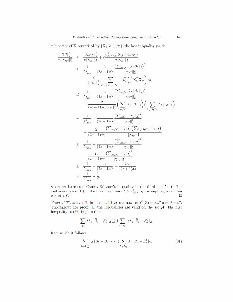
Y. Nardi and A. Rinaldo/The log-linear group lasso estimator 626
submatrix of X comprised by {Xh, h ∈ H′}, the last inequality yields
‖Xβ‖22
n‖γH′‖22
≥ ‖XβH′‖22
n‖γH′‖22
+ 2β⊤H′X⊤
H′X(H′)cβ(H′)c
n‖γH′‖22
≥ 1
λ2max
− 1
(2c + 1)δs
(∑h∈H′ λh‖βh‖2
)2
‖γH′‖22
− 2
‖γH′‖22
∑
h∈H′ ,h′∈(H′)c
β⊤h
(1
nX⊤
h Xh′
)βh′
≥ 1
λ2max
− 1
(2c + 1)δs
(∑h∈H′ λh‖βh‖2
)2
‖γH′‖22
− 2
(2c + 1)δs‖γH′‖22
(∑
h∈H′
λh‖βh‖2
)( ∑
h∈(H′)c
λh‖βh‖2
)
=1
λ2max
− 1
(2c + 1)δs
(∑h∈H′ ‖γh‖2
)2
‖γH′‖22
− 2
(2c + 1)δs
(∑h∈H′ ‖γh‖2
) (∑h∈(H′)c ‖γh‖2
)
‖γH′‖22
≥ 1
λ2max
− 1
(2c + 1)δs
(∑h∈H′ ‖γh‖2
)2
‖γH′‖22
− 2c
(2c + 1)δs
(∑h∈H′ ‖γh‖2
)2
‖γH′‖22
≥ 1
λ2max
− s
(2c + 1)δs− 2cs
(2c + 1)δs
≥ 1
λ2max
− 1
δ,
where we have used Cauchy-Schwarz’s inequality in the third and fourth lineand assumption (U) in the third line. Since δ > λ2
max by assumption, we obtainκ(s, c) > 0.
Proof of Theorem 4.5. In Lemma 6.1 we can now set f0(X) = Xβ0 and β = β0.Throughout the proof, all the inequalities are valid on the set A. The firstinequality in (37) implies that
∑
h
λλh‖βh − β0h‖2 ≤ 4
∑
h∈H0
λλh‖βh − β0h‖2,
from which it follows
∑
h∈Hc0
λh‖βh − β0h‖2 ≤ 3
∑
h∈H0
λh‖βh − β0h‖2. (31)

Y. Nardi and A. Rinaldo/The log-linear group lasso estimator 627
Similarly, using the second inequality in (37),
1
n‖X(β − β0)‖2
2 ≤ 4λ√|H0|
√∑
h∈H0
λ2h‖βh − β0
h‖22. (32)
Combining (31) and (32), and using assumption (RE(|H0|, 3)), we obtain
√∑
h∈H0
λ2h‖β − β0‖2
2 ≤ 4λ√
|H0|κ2
0
, (33)
which yields (11).Next, in virtue of (33), and using Cauchy-Schwarz’s inequality
∥∥∥Λ(β − β0)∥∥∥
2≤
∑
h
λh‖β − β0‖2 ≤ 4∑
h∈H0
λh‖β − β0‖2
≤ 4√|H0|
√∑
h∈H0
λ2h‖β − β0‖2
2,
which is bounded by 16 λκ20
|H0|. This implies
‖β − β0‖2 ≤ 16λ
κ20λmin
|H0|,
which is (10).In order to show (12), we first show that
|H| ≤ 16
9
Cmax
λ2λ2min
1
n‖X(β0 − β)‖2
2. (34)
From the subgradient conditions, we get, for each h,
1
nX⊤
h
(X(β0 − β)
)+
1
nX⊤
h ǫ = λλhzh,
where zh = βh
‖βh‖2
if βh 6= 0 and zh is any vector with ℓ2 norm bounded by 1 if
βh = 0. Then, by the triangle inequality,
1
n
∥∥∥X⊤h
(X(β − β0)
)∥∥∥2≥ λλh − 1
n
∥∥X⊤h ǫ∥∥2≥ 1
2λλh,
for each h. It then follows that
1
n2
∑
h∈H
∥∥∥X⊤h
(X(β − β0)
)∥∥∥2
2≥ |H|λ2λ2
min
1
4. (35)
On the other hand, since
XX⊤ =∑
h
XhX⊤h ,

Y. Nardi and A. Rinaldo/The log-linear group lasso estimator 628
we also have
1
n2
∑
h∈H
∥∥∥X⊤h
(X(β − β0)
)∥∥∥2
2≤ 1
n2
(X(β − β0)
)⊤XX⊤
(X(β − β0)
)
≤ Cmax
n‖X(β − β0)‖2
2, (36)
where the last inequality follows from the fact that 1nX⊤X and 1
nXX⊤ have thesame maximal eigenvalue. Combining (35) and (36),
|H| ≤ 4Cmax
λ2λ2min
1
n‖X(β0 − β)‖2
2,
which is (34). Inserting equation (11) in (34), we obtain (12).
Proof of Theorem 4.7. Following the results of section A, part IV of Zhou et al.(2007), assumptions (P1) and (P2) coupled with Berstein’s inequality yield
maxj,k
∣∣∣Σj,k − Σj,k
∣∣∣ = OP
(√log n
n
).
Then,
supβ∈Bn
|R(β) − R(β)| = supβ∈Bn
∣∣∣γ⊤(Σ − Σ)γ∣∣∣
≤ supβ∈Bn
maxj,k
∣∣∣Σj,k − Σj,k
∣∣∣ ‖γ‖21
≤ supβ∈Bn
∣∣∣Σj,k − Σj,k
∣∣∣
(1 +
∑
h
√dh‖βh‖2
)2
≤ maxj,k
∣∣∣Σj,k − Σj,k
∣∣∣ (1 + bn)2
= oP (1).
where, in the second inequality, we used the bound ‖γ‖1 ≤ 1 +∑
h
√dh‖βh‖2
and the last step follows from (15). Therefore,
supβ∈Bn
|R(β) − R(β)| p→ 0,
which implies persistence with respect to {Bn}, since
|R(βn) − infβ∈Bn
R(β)| ≤ 2 supβ∈Bn
|R(β) − R(β)|.
The second part of the statement follows for the simple chain of inequalities∑
h
√dh‖βh‖2 =
∑
h
√dh‖βh‖2I{βh 6=0}
≤ ‖β‖2
√∑
h
dhI{βh 6=0}
≤ C√
dmax
√|{h, βh 6= 0}|,

Y. Nardi and A. Rinaldo/The log-linear group lasso estimator 629
where ‖β‖2 ≤ C holds uniformly over n for some constant C in virtue of (P1)and the assumed positivity of the minimal eigenvalue of the covariance matrix ofthe predictors. Under (16), this implies Cn ⊂ Bn for each n and thus persistencywith respect to {Cn}n.
6. Appendix
Proof of Lemma 4.3. Let Vh = 1√nσ
X⊤h ǫ, so that Vh ∼ Ndh
(0, I) and ‖Vh‖22 ∼
χ2dh
. By the union bound,
P(Ac) ≤∑
h
P
(‖Vh‖2
2 ≥ 1
4
n
σ2λ2λ2
h
)=∑
h
P
(‖Vh‖2
2 − dh ≥ 1
4
n
σ2λ2λ2
h − dh
)
=∑
h
P
(‖Vh‖2
2 − dh ≥√
2dhxh
),
where xh = 1√2
(14
n
σ2 λ2λ2h√
dh−√
dh
). For large enough n, we can apply the tail
bound inequality for a variable distributed like χ2dh
(see, e.g. Cavalier et al.,2002), yielding
P(Ac) ≤∑
h
exp
− x2h
2(1 + xh
√2
dh
)
.
Because of (A), for large enough n,
exp
{− x2
h
2(1 + xh
√2
dh
)}
≤ exp
{− x2
h
3√
2 xh√dh
}= exp
{− 1
3√
2
( n
σ2λ2λ2
h − dh
)},
from which it follows, once again using (A), that
P(Ac) ≤ exp
{log |H| − 1
3√
2min
h
( n
σ2λ2λ2
h − dh
)}→ 0.
This concludes the proof.
Lemma 6.1. Let EY = f0(X), for some function f0 and assume (N). On theevent A, for any β ∈ R
d with block support set H′ = {h : βh 6= 0},
1
n‖Xβ − f0(X)‖2
2 +∑
h
λλh‖βh − βh‖2
≤ 1
n‖Xβ − f0(X)‖2
2 + 4λ∑
h∈H′
λh‖βh − βh‖2
≤ 1
n‖Xβ − f0(X)‖2
2 + 4λ√|H′|
√∑
h∈H′
λ2h‖βh − βh‖2
2, (37)

Y. Nardi and A. Rinaldo/The log-linear group lasso estimator 630
Proof of Lemma 6.1. Following the derivation in Bunea et al. (2007a), for anarbitrary β ∈ R
d with block support set H′, it holds that
1
2n‖Xβ − f0(X)‖2
2 ≤ 1
2n‖Xβ − f0(X)‖2
2 +∑
h
λλh‖βh‖2
−∑
h
λλh‖βh‖2 +∑
h
W⊤h (βh − βh), (38)
where Wh = 1nX⊤
h ǫ. By Cauchy-Schwarz’s inequality, on the event A,
∑
h
|W⊤h (βh − βh)| ≤ 1
2
∑
h
λλh‖βh − βh‖2. (39)
Using the last display, and adding and subtracting 12
∑h λλh‖βh−βh‖2 to both
sides of (38), the term
1
2n‖Xβ − f0(X))‖2
2 +1
2
∑
h
λλh‖βh − βh‖2
is bounded by
1
2n‖Xβ − f0(X)‖2
2 +∑
h
λλh‖βh − βh‖2 +∑
h
λλh‖βh‖2 −∑
h
λλh‖βh‖2,
which, in turn, is no larger than
1
2n‖Xβ − f0(X)‖2
2 +∑
h∈H′
λλh‖βh − βh‖2 +∑
h∈H′
λλh
(‖βh‖2 − ‖βh‖2
),
all the above inequalities being valid on A. Then, from (38), and applying thetriangle inequality to the last display, we obtain, still on A,
1
2n‖Xβ − f0(X)‖2
2 +1
2
∑
h
λλh‖βh − βh‖2
≤ 1
2n‖Xβ − f0(X)‖2
2 + 2λ∑
h∈H′
λh‖βh − βh‖2
≤ 1
2n‖Xβ − f0(X)‖2
2 + 2λ√|H′|
√∑
h∈H′
λ2h‖βh − βh‖2
2,
where the second inequality stems from Cauchy-Schwarz’s inequality. The lastexpression, multiplied by 2, is (37).
7. Acknowledgments
We thank the anonymous referees and, in particular, the associate editor fordetailed and constructivce comments that led to a much improved presentation.

Y. Nardi and A. Rinaldo/The log-linear group lasso estimator 631
References
Bach, F. (2007). Consistency of the group Lasso and multiple kernel learning,to appear in Journal of Machine Learning.
Bickel, P.J., Ritov, Y. and Tsybakov, A. B. (2007). A Simultaneous analysis ofLasso and Dantzig selector. Submitted to Annals of Statistics.
Bunea, F., Tsybakov, A. B. and Wegkamp, M. H. (2007). Aggregation for Gaus-sian regression, The Annals of Statistics, 35(4), 1674–1697. MR2351101
Bunea, F., Tsybakov, A. and Wegkamp, M. (2007b). Sparsity oracle inequalitiesfor the lasso, Electronic Journal of Statistics, 1, 169–194. MR2312149
Cavalier, L., Golubev, G. K., Picard, D. and Tsybakov, A. B. (2002). Oracleinequalities for inverse problems, Annals of Statistics, 30 843–874. MR1922543
Dahinden, C., Parmiggiani, G., Emerick, M.C. and Buhlmann, P. (2006). SparseContingency Tables and High-Dimensional Log-Linealr Models for AlternativeSplicing in Full-Length cDNA Libraries, Research Report 132, Swiss FederalInstitute of Technology.
Efron, B., Hastie, T., Johnstone, I. and Tibshirani, R. (2004). Least angle re-gression, Annals of Statistics, 32, 407–499. MR2060166
Fan, J. and Li, R. (2001). Variable selection via non-concave penalized likelihoodand its oracle properties, Journal of the American Statistical Association,96(456), 1348–1360. MR1946581
Fan J. and Peng, H. (2004). Nonconcave penalized likelihood with a divergingnumber of parameters, Annals of Statistics, 32(3), 928–961. MR2065194
Geyer, C. (1994). On the asymptotics of constrained-M estimation, Annals ofStatistics,, 22, 1993–2010. MR1329179
Gilbert, A. C. and Strauss, M. J. (2006). Algorithms for Simultaneous SparseApproximation Part II: Convex Relaxation, Signal Processing, 86, 572–588
Greenshtein, E. and Ritov, Y. (2004). Persistence in high-dimensional predic-tor selection and the virtue of overparametrization, Bernoulli, 10, 971–988.MR2108039
Greenshtein, E. (2006). Best subset selection, persistence in high-dimensionalstatistical learning and optimization under ℓ1 constraint, Annals of Statistics,34(5), 2367–2386. MR2291503
Kim, Y., Kim, J. and Kim, Y. (2006). Blockwise sparse regression. StatisticaSinica, 16(2). MR2267240
Knight, K. and Fu, W. (2000). Asymptotics for Lasso-type estimators, Annalsof Statistics, 28(5), 1356–1378. MR1805787
Koltchinskii, V. (2005). Sparsity in Penalized Empirical Risk Minimization,manuscript.
Ledoux, M. and Talagrand, M. (1991). Probability in Banach spaces: isoperime-try and processes. Springer-Verlag. MR1102015
Lounici, K. (2008). Sup-norm convergence rate and sign concentration propertyof Lasso and Dantzig estimators, Electronic Journal of Statistics, 2, 90–102.MR2386087
Massart, P. (2007). Concentration Inequalities and Model Selection, LectureNotes in Mathematics, Vol. 1896, Springer. MR2319879

Y. Nardi and A. Rinaldo/The log-linear group lasso estimator 632
Meier, L., van der Geer, S. and Buhlmann, P. (2006). The Group Lasso forLogistic Regression, Journal of the Royal Statistical Society, Series B, 70(1),53–7.
Meinshausen, N. and Buhlmann, P. (2006). High dimensional graphs andvariable selection with the lasso, Annals of Statistics, 34(3), 1436–1462.MR2278363
Meinshausen, N. and Yu, B. (2006). Lasso-type recovery of sparse representa-tions for high-dimensional data, to appear in the Annals of Statistics.
Nardi, N. and Rinaldo, A. (2007). The Log-linear Group-Lasso Estimator andIts Asymptotic Properties, manuscript.
Osborne, M.R., Presnell, B. and Turlach, B.A. (2000). On the LASSO andits Dual, Journal of Computational and Graphical Statistics, 9(2), 319–337.MR1822089
Portnoy, S. (1988). Asymptotic behavior of likelihood methods for exponentialfamilies when the number of parameters tends to infinity, Annals of Statistics,16(1), 356–366. MR0924876
Ravikumar, P., Lafferty, J., Liu, H. and Wasserman, L. (2007). Sparse AdditiveModels, manuscript.
Rinaldo (2006). Computing Maximum Likelihood Estimates in Log-Linear Mod-els, Technical report, Department of Statistics, Carnegie Mellon University.
Tibshirani, R. (1996). Regression shrinkage and selection via the lasso, Journalof the Royal Statistical Society, Series B, 58(1), 267–288. MR1379242
van de Geer, S.A. (2007). Oracle inequalities and Regularization, in Lectures onEmpirical Processes, European Mathematical Society. MR2284824
van der Vaart, A.W. and Wellner, J.A. (1998). Weak Convergence and EmpiricalProcesses, Springer.
Wainwright, M. J. (2006). Sharp thresholds for high-dimensional and noisy re-covery of sparsity, Technical Report 708, Department of Statistics, UC Berke-ley.
Wainwright, M. J. (2007). Information-theoretic limits on sparsity recovery inthe high-dimensional and noisy setting, Technical Report, UC Berkeley, De-partment of Statistics.
Yuan, M. and Lin Y. (2006). Model selection and estimation in regression withgrouped variables, Journal of the Royal Statistical Society, B, 68(1), 49–67.MR2212574
Yuan, M. and Lin Y. (2006). On the non-negative garrotte estimator, Journalof the Royal Statistical Society, B, 69(2), 143–161. MR2325269
Zhang, T. (2007). Some Sharp Performance Bounds for Least Squares Regressionwith L1 Regularization, manuscript.
Zhang, H. and Huang, J. (2007). The sparsity and bias of the Lasso selection inhigh-dimensional linear regression, to appear in the Annals of Statistics.
Zhao, P., Rocha, G. and Yu, B. (2008). Grouped and hierarchical model selectionthrough composite absolute penalties, manuscript.
Zhao, P. and Yu, B. (2006). On Model Selection Consistency of Lasso, Journalof Machine Learning Research, 7, 2541–2563. MR2274449

Y. Nardi and A. Rinaldo/The log-linear group lasso estimator 633
Zhou, S., Lafferty, J. and Wasserman, L. (2007). Compressed Regression,manuscript.
Zhou, N. and Zhu, J. (2007). Group Variable Selection via Hierarchical Lassoand Its Oracle Property, manuscript.
Zou, H. (2006). The adaptive lasso and its oracle properties, Journal of theAmerican Statistical Association, 101(476), 1418–1429. MR2279469
H. Zou and T. Hastie. Regularization and variable selection via the elasticnet, Journal of the Royal Statistical Society, Series B, 67(2):301–320, 2005.MR2137327


![Algebraic Statistics for a Directed Random Graph Model with ...stat.cmu.edu/~arinaldo/papers/OFFPRINT-PAPER-conm10180.pdflanguage of algebraic statistics. See, e.g., [7, 16]and[8]](https://img.dokumen.tips/doc/110x75/5f70cab788c5e5758f163d28/algebraic-statistics-for-a-directed-random-graph-model-with-statcmueduarinaldopapersoffprint-paper-.jpg)