On the analysis of ”simple” 2D stochastic cellular automata

Damien Regnault1, Nicolas Schabanel1,2, and Eric Thierry1,3

1 IXXI – LIP, Universite de Lyon, Ecole Normale Superieure de Lyon, 46 allee d’Italie, 69364 Lyon Cedex07, France. http://perso.ens-lyon.fr/{damien.regnault,eric.thierry}.

2 CNRS, Centro de Modelamiento Matematico, Universidad de Chile, Blanco Encalada 2120 Piso 7,Santiago de Chile, Chile. http://www.cmm.uchile.cl/∼schabanel.

3 CNRS, Laboratoire d’Informatique Algorithmique: Fondements et Applications, Universite Paris 7,75205 Paris Cedex 13.

Abstract. Cellular automata are usually associated with synchronous deterministic dynam-ics, and their asynchronous or stochastic versions have been far less studied although signifi-cant for modeling purposes. This paper analyzes the dynamics of a two-dimensional cellularautomaton, 2D Minority, for the Moore neighborhood (eight neighbors per cell) under fullyasynchronous dynamics (where only one random cell updates at each time step). Even if 2DMinority seems a simple rule, from the experience of Ising models and Hopfield nets it isknown that models with negative feedback are hard to study.This automaton actually presents a rich variety of behaviors, even more complex that whathas been observed and analyzed in a previous work on 2D Minority for the von Neumannneighborhood (four neighbors per cell) [1]. This paper confirms the relevance of the approachof [1] (definition of energy functions and identification of competing regions) but switching tothe Moore neighborhood complicates a lot the description of intermediate configurations. Newphenomena appear (particles, wider range of stable configurations). Nevertheless we manageto analyze different stages of the dynamics. It suggests that predicting the behavior of thisautomaton although difficult is possible, opening the way to the analysis of the whole classof totalistic automata.

1 Introduction

Cellular automata are attractive models for complex systems in various fields, like physics, biologyor social sciences. Their relevance is supported by many observations of natural phenomena whichclosely match the dynamics of some cellular automaton, as illustrated by Fig. 1. An example ofchallenging issue in biology is to predict the expression of genes in a set of cells which share thesame gene regulatory network. Cellular automata can be used to model such systems [2, 3]. Forexample consider the simple gene regulatory networks where a gene exerts a feedback inhibition ofits expression. The state of a cell is whether it expresses this gene or not. Assuming that each cellstarts expressing the gene when less than half of its neighbors (including itself) express it, and thatotherwise it stops expressing it, leads to the Minority rule [4]. If cells are assembled into a two-dimensional grid, it yields 2D Minority. Such a model is of course an extreme simplification of anyreal phenomena but understanding this ”simple” model is already an indispensable step towardsthe study of more involved interaction networks. Surprisingly, it already exhibits an astonishinglyrich behavior which is investigated in this paper.

The 2D Minority automaton belongs to the class of threshold cellular automata which havebeen intensively studied under synchronous dynamics (at each time step, all the cells update simul-taneously) [5]. However models for natural phenomena rather update asynchronously. Empirical

2

1.a – The pattern growth of the shell of the widespreadspecies Conus textile is governed by a mathematical func-tion presenting similarities with the Rule 30 CA above.

1.b – 2D minority induced by a set of cells ex-pressing (in black) or not (in white) a gene whichtends to inhibit its expression in neighboring cells.

Fig. 1. Cellular automata as models in biology.

studies [6–11] have shown how the behavior can change drastically when introducing asynchronism.However only few mathematical analyses are available and they mainly concern one-dimensionalstochastic cellular automata [12–15]. Providing analyses of 2D rules remains a real challenge. Forinstance the mean-field approach does not succeed in approximating tightly such stochastic dynam-ics [16]. Fig. 2 illustrates for three 2D cellular automata the differences between the synchronousdynamics and the fully asynchronous dynamics where only one random cell updates at each timestep. Some related stochastic models like Ising models or Hopfield nets have been studied underasynchronous dynamics (our model of asynchronism corresponds to the limit when temperaturegoes to 0 in the Ising model). These models are acknowledged to be harder to analyze when itcomes to two-dimensional topologies [17] or negative feedbacks [18].

For all these reasons 2D Minority under fully asynchronous dynamics turns out to be an in-teresting and challenging candidate for mathematical analyses. This paper focuses on the Mooreneighborhood: at each time step, the fired cell updates to the minority state among its eight closestneighbors and itself. It carries on a work initiated in [1] where 2D Minority was analyzed for thevon Neumann neighborhood (four neighbors instead of eight). One might have hoped for minorsadjustments to deal with the Moore neighborhood, however the results do not come out so easily.Experiments discussed in Section 3 show that new patterns (wider variety of striped patterns) andnew phenomena occur (particle-like behaviors). Several key ideas presented in [1] (energy, bordersand regions) apply, but their use requires some innovations. We show that the initial stage of thedynamics is characterized by a fast energy drop (Theorem 3). We exhibit borders that separatestriped regions competing with one another and we manage to prove how final stable (horizontally

Life a random Totalistic Minority

Synchronousdynamics

Fullyasynchronous

dynamics

Fig. 2. Typical configurations observed during the evolution of some 2D cellular automata (Moore neighbor-hood). Similar stripes emerge in asynchronous regime even if their synchronous behavior differ drastically.

3

or vertically) stripes configurations are reached almost surely from typical configurations occur-ing at the end of the process. Furthermore, we prove that this convergence occurs in polynomialtime (Theorem 5). In the proof, we show that as the regions crumble, inflate or retract, the over-all structure admits a recursive description which persists over time. The proofs of the study ofsuch dynamical systems, know as complex systems, involve unavoidable tedious case studies andone of the important contribution of this paper is to set up a compact, possibly elegant, and thussafe framework to deal with these enumerations of cases. Note that in the course of the paper, wepresent an interesting characterization of the stable configurations for 2D Minority for the Mooreneighborhood (Theorem 2). As far as we know, it had only been solved for the von Neumannneighborhood [5].

2 Definitions

We consider in this paper the 2D 2-states cellular automaton Minority under fully asynchronousdynamics over finite configurations with periodic boundary conditions.

Definition 1 (Configuration). We are given two positive integers n and m, let N = nm. Wedenote by T = Zn×Zm the set of cells and Q = {0, 1} the set of states (0 stands for white and 1 forblack in the figures). We consider the Moore neighborhood: two cells (i, j) and (k, l) are neighborsif max(|i − k|n, |j − l|m) 6 1 (where |i − j|p denotes the distance in Zp). A n ×m-configuration cis a function c : T→ Q; cij is the state of the cell (i, j) in configuration c.

Definition 2 (Stochastic 2D Minority). We consider the fully asynchronous dynamics of 2DMinority. Time is discrete and let ct denote the configuration at time t; c0 is the initial configuration.The configuration at time t+ 1 is a random variable defined by the following process: a cell (i, j) isselected uniformly at random in T and its state is updated to the minority state in its neighborhood(we say that cell (i, j) fires at time t), all the other cells remain in their current state:

ct+1ij =

1 if (ctij+c

ti−1,j + cti+1,j + cti,j−1 + cti,j+1

+cti−1,j+1 + cti−1,j−1 + cti+1,j−1 + cti+1,j+1) 6 40 otherwise

and ct+1kl = ctkl for all (k, l) 6= (i, j). A cell is said active if its state would change if fired.

Definition 3 (Convergence). A configuration c is stable if it remains unchanged under the dy-namics, i.e., if all its cells are inactive. We say that the random sequence (ct) converges almostsurely from an initial configuration c0 = c if the random variable T = min{t : ct is stable} is fi-nite with probability 1. We say that the convergence occurs in polynomial time on expectation ifE[T ] 6 p(N) for some polynomial p.

3 Experiments

Typical behavior. Like other 2D automata (such as Game of Life [6, 19]), the asynchronous behaviorof 2D Minority differs radically from its synchronous dynamics. In particular, [5] proved that thesynchronous dynamics eventually leads to stable configurations or cycles of two opposite configu-rations. The latter case is the typical behavior in synchronous simulations where one can observe

4

initial config. step 1N step 5N step 10N step 20N step 30N step 50N

step 70N step 90N step 100N step 120N step 130N step 140N step 153N

Fig. 3. A typical execution of stochastic 2D Moore minority with N = 50× 50 cells.

big flashing islands (Fig. 2). On the contrary, as can be observed in Fig. 3, the states of most ofthe cells are very stable over time in fully asynchronous regime and present typically very rapidlystriped patterns (horizontal or vertical) that tend to extend and merge with each other until onegets over the others and covers the whole configuration (when at least one of the dimensions n orm is even). A goal of this paper is to explore how such stripes arise and end up covering the wholeconfiguration. Note also that such stripes arise as well in many other asynchronous automata suchas the totalistic cellular automata (see Section 1). Very rarely a random initial configuration mayconverge to more exotic stable configurations. Fig. 7 gives some examples of more or less exoticstable configurations under 2D minority dynamics.

Borders and Particles. Part of the richness of 2D Minority under fully asynchronous behavior isdue to some specific configurations where ”particles” can be observed. Several patterns can beidentified as particles although for now we do not have a formal definition. We say that there is aborder between two diagonally neighboring cells if they are in the same state (more details in thenext section). Active cells are always located near the borders. When the borders draw a pattern

(where red spots indicate active cells), then, depending of which of the two active cell fires

the pattern will move in different directions: forward or backward . Such patterns which”move” along borders can be called particles. In some configurations, the set of all the borders forma network of ”rails” carrying several particules. These particules follow random walks along the railsand vanish when they collide. Note that the dynamics is a lot more intricate than 2D random walks

4.a – A sequence of updates in a configu-ration starting with 4 particles where twoof them move along rails and ultimatelyvanish after colliding with each other.

4.b – A sequence of updates where the rails cannot sus-tain the pertubations due to the movements of the parti-cles: at some point, rails get to close with each other, newactive cells appear, and part of the rail network collapses.

Fig. 4. Some examples of the complex behavior of particles in a 20 × 20 configuration.

5

Fig. 5. A typical 16 × 32 toric configuration after 3N fully asynchronous steps, with its blue and greenborders and diamonds.

because the rails are modified by the passage of the particules and if two rails become too close, awhole part of the rail network collapses. Fig. 4 illustrates this kind of phenomena. Configurationswith particles and rails are rarely reached from a random initial configuration. Nevertheless, wehave to consider them when we study the convergence and these phenomena are extremely difficultto analyze mathematically. Such a system of particles is not observed in asynchronous 2D minoritywith von Neumann neighborhood [1] or in related models like the ferromagnetic Ising model orHopfield networks with positive feedback.

4 Energy, Borders, Diamonds and Stable Configurations

4.1 Borders, Diamonds and Stripes

The following definitions allow to highlight the underlying structure of a configuration with respectto the dynamics. These tools turn out to be a key step to prove the convergence. Note that as opposedto the von Neumann neighborhood in [1], the definition of the borders is no longer straightforwardfrom the transition table for the Moore neighborhood.

Definition 4 (Stripes). If n and m are even, a set of cells R is said to be tiled with even horizontalstripes (resp. odd horizontal, even and odd vertical stripes) if cij = i mod 2 (resp. i + 1, j,j+1 mod 2), for all cell (i, j) ∈ R. Note that cells whose whole neighborhood is striped are inactive.

Definition 5 (Borders and diamonds). We say that there is a border between two diagonallyneighboring cells (i, j) and (i + ε, j + η), with ε, η ∈ {−1, 1}, if they are in the same state, i.e., ifcij = ci+ε,j+η.

If n and m are even, we say that a cell (i, j) is even (resp. odd) if i+ j is even (resp. odd). Wesay that the border between two cells is blue if the cells are even, and green otherwise; furthermore,we say that there is a diamond over cell (i, j) if its state coincides with even horizontal stripes, i.e.,if cij = i mod 2; the diamond is blue if the cell is even and green otherwise (see Fig. 5).

Proposition 1 (Borders are boundaries). The borders are the exact boundary of regions tiledwith stripes patterns (odd/even horizontal/vertical). Moreover, when n and m are even, the blue(resp. green) borders are the exact boundary of the regions covered by the blue (resp. green) diamonds.

6

Since cells whose neighborhood is striped are inactive, the only active cells in a configurationmay be found along the borders.

4.2 Energy

As in Ising model [17] or Hopfield networks [18], we define a natural global parameter that onecan consider to be the energy of the system since it counts the number of interactions betweenneighboring cells in the same state. This parameter will provide key insights on the evolution of thesystem.

Definition 6 (Potential). The potential vij of cell (i, j) is the number of its neighboring cells inthe same state as itself minus 2.4 By definition, if vij 6 1, then the cell is in the minority statein its own neighborhood and is thus inactive (its state will not change if fired); whereas, if vij > 2then the cell is active and its state will change if fired. Note that a configuration c is stable iff forall cell (i, j) ∈ T, vij 6 1.

Definition 7 (Energy). Let say that a subset of cells R is fat if for each cell (i, j) ∈ R, thereexists a square Q = {(i, j), (i + ε, j), (i + ε, j + η), (i, j + η)}, for some ε, η ∈ {1,−1}, such thatQ ⊂ R. The energy ER of set R in a given configuration is defined as: ER =

∑(i,j)∈R vij. We

denote by E the energy of the whole configuration c.

The next proposition shows that the energy is non-negative for almost every subset of cells of aconfiguration. This means that there cannot be too many cells with negative potential. This impliesthat the decrease of energy over time (Proposition 3 and Theorem 3) is not due to the increase ofthe number of cells with negative potential, but to the decrease of the potentials of the cells withpositive potential, which explains intuitively why the striped patterns which have minimum energy(Proposition 4) arise naturally very rapidly.

Proposition 2 (Energy is non-negative). For any fat subset of cells R of size q: 0 6 ER 6 6q.

The following easy fact will be very handy in order to prove the convergence of the dynamics.

Fact 1. When an active cell (i, j) is fired, its new potential is vij := 4 − vij and the total energyvaries by 8− 2vij. Note that if vij = 2, both remain unchanged.

Proposition 3 (Energy is non-increasing). Under fully asynchronous dynamics, the energy isa non-increasing function of time and decreases each time a cell with potential > 3 fires.

Striped configurations are stable and correspond to the minimum energy configurations.

Proposition 4 (Minimum energy configurations). The energy of a configuration c is 0 iff cis a striped configuration.

4.3 Stable Configurations

As opposed to the von Neumann fully asynchronous dynamics in [1], stable configurations underthe Moore neighborhood exhibit rather complex structures as shown on Fig. 7. Although thereis a great variety of stable configurations, a general structure can be extracted and they can becharacterized thanks to the borders. We first describe the stable configurations when n and m areeven and deduce from there the structure of the stable configurations in the general case by doublingthe odd dimension. Fig. 6 gives examples of each type of stable configurations.4 The offset −2 is convenient since its ensures that the minimum energy of a configuration is 0 (see

Proposition 2 below).

7

H

H' H'

V

V'

V

V'

HH'

V'

V V'

H

V

H'

A

C

A'

C

A'

B'C

A A

B'

C

A'

B

B'

A'

A

a 16 × 32 stable configuration of type III(the columns (in the underlying grid) of odd width regions are highlighted in red)

an 11 × 22 stable configuration of type I

an 11 × 22 stable configuration of type II

H

H'

H'

V

V V'

H

V'

A'A'

D

A

D

D

A

D

a 7 × 24 stable configuration of type III(odd height regions are highlighted in red)

Fig. 6. Examples of stable configurations illustrating most of the possibilities.

Theorem 2 (Stable configurations). When at least one of n and m is even, there are exactlythree types of stable configurations:

– Type I: the borders are parallel straight (diagonal) lines such that: two lines of the same colorare at (`1-)distance > 2; if two lines blue and green are at distance 1, there is no other lineat distance 6 4 from each of them; the number of lines of each color along each row (resp.,column) of the configuration has the same parity as m (resp., n).

– Type II: all the blue and green borders are all pairwise interlaced either horizontally according tothe pattern , or vertically according to ; the pairs of interlaced borders are at distance > 2from each other; and the number of interlaced pairs has the parity of n if interlaced horizontally,and of m otherwise.

– Type III: the borders define a bicolor (horizontal/vertical stripes) underlying toric grid s.t.:

horizontal stripes

horizontal stripes

horizontal stripes

horizontal stripes

vertical stripes

vertical stripes

vertical stripes

vertical stripes

horizontal stripes

horizontal stripes

horizontal stripes

horizontal stripes

vertical stripes

vertical stripes

vertical stripes

vertical stripes

Crossings between green and blue bordersStraight (diagonal) blue or green borders

• the segments of borders between two intersections are straight linesat distance at least 2 from each other;• two borders of the same color cannot intersect;• the number of borders of each color crossed by every row (resp. col-

umn) in the configuration has the same parity as m (resp. n);• the borders of opposite colors intersect at the corners of the cells only,

and according to the following (possibly overlapping) patterns:

/ Region of where each column of cells has an even/odd height

and / (resp. and / ) denote horizontally (resp. vertically) striped region of identical/opposite parity

/ Region of where each row of cells has an even/odd length

H H V'VH' V and denote borders of opposite colors

evenheight

evenwidth

evenheight

evenwidth

evenheight

evenwidth

evenheight

evenwidth

evenheight

even width

evenheight

odd widthodd

height

even width

SYM

ROT, 0/1

ROT, 0/1H

V

H'

V'

A'

H

V

H'

V'

Type

H

V

H'

V'

ROT, SYM, 0/1

AType

H

V

H'

V'

BType

SYM, 0/1

ROT H

V

H'

V'

SYM, 0/1

B'Type

even number of turns (zero or more) for each border

odd number of turns (one or more)for each border

H

V

H

V'

H

V

H'

V

CType DType

ROT

SYM, 0/1

SYM, 0/1

... ... ... ...

Furthermore, no stable configuration can have both crossings of types C and D and if a regionhas a crossing of type C (resp., D), all the crossings at the same vertical (resp., horizontal)level in the underlying grid are of type C (resp., D); moreover, the partity of the number of suchhorizontal (resp., vertical) levels of C-crossings (resp., D-) equals the parity of m (resp. n).

8

E = 0 Low E Higher E Med E High E The four highest energy config. (E = N)

Fig. 7. Examples of stable configurations for 2D Minority at various levels of energy.

And any n×m-configuration of type I, II or III is a stable configuration.

Corollary 1. If n and m are odd, no stable configuration exists, and the dynamics never converges.If only one of n and m is odd, stable configurations of type A, B, and C exist with the parityrestrictions mentioned in Theorem 2.

Proposition 5 (Stable configurations energy). The energy of a stable configuration c satisfies:0 6 E 6 N . The only configurations with minimum energy (zero) are tiled with a striped 1 × 2-pattern. And the only stable configuration with maximum energy N are of four types: either tiled

with the 2× 4-pattern , or the 8× 8-patterns ,

D4

D5

D6

D10

D5

D6

D4D4

D4

D4

D4

D10D10

D10D10

D4

D4

D4D6

D6

D6

D6

D5 ou

D6

D5 ou

D6

D5

D8D8

D5

D8

D8 D8D8

D5

D10D5

D4

D4

D4D10D4 D5 , or (see Fig. 7).

5 Analysis of the convergence

In this section, we give our results on the existence and speed of the convergence of the dynamics to-wards a stable configuration from an arbitrary initial configuration. As opposed to the von Neumandynamics where we were able to analyse the whole convergence, because of the existence of particlesfollowing sophisticated guided random walks (see Section 3), we are only able to describe the firststeps and the last steps of the convergence. These results rely on the study of the energy functionwhich is combined with an other parameter to obtain a variant. This variant allows to reduce thestudy of the randomly evolving 2D shape to an one dimensional random walk. The section endswith challenging conjectures on the overall convergence of the process.

5.1 Initial energy drop

According to experiments, the energy of a configuration drops very fast during the first steps untilit converges, most of the time to a striped configuration of minimal energy. The following theoremprovides a bound on the speed of this initial energy drop.

Theorem 3. The energy of any configuration of size N is at most N + 2N/3 after O(N2) fullyasynchronous minority updates on expectation.

5.2 The last steps of convergence

From now on, we assume that n and m are even. As mentioned above, in most of the experimentsstriped regions arise quickly, then they extend, compete with each other, merge until only onecovers the whole configuration. In this section, we provide an analysis of the very last steps of theconvergence to this stable configuration: the case where there remains only one single horizontallystriped region within a vertically striped background, which we will call a standard configuration.

9

We then show that the background ends up covering the whole configuration in polynomial timeon expectation as expected according to the experiments (Fig. 3 when t > 100N). This involvesstudying the randomly evolving shape defined by the horizontal striped regions.

Note that every configuration is completely determined by its set of diamonds. When startingfrom what we call a standard configuration (Definition 9) seen as a set of diamonds, we analyze howadditions/deletions of diamonds occur and how the set evolves. We observe that the islands of greenor blue diamonds (Definition 10) extend from the hollows of their boundaries and are dug from theircorners. Once disclosed the structure of the set of islands (valid configurations recursively describedin Definition 11 and Fig. 8), we show by studying a combination of the energy with the area of therandom shape, that the random shape of the set of diamonds tends to vanish. Interestingly enough,we show that the horizontally striped region can flip the parity of its stripes but cannot extendbeyond its initial surrounding rectangle (Definition 8).

Definition 8 (Surrounding rectangles). A blue rectangle (resp. green rectangle) is a rectanglesuch that its sides are parallel to the diagonals and its corners are located at the centers of odd(resp. even) cells. A blue or green rectangle is enclosing a set of diamonds D if all the diamondsare contained in the rectangle, and it is surrounding D if it is the smallest enclosing rectangle ofthat color for D.

Definition 9 (Standard initial configuration). We say that a configuration is standard if itconsists in a finite set of diamonds of the same color forming a rectangle (i.e., a set of diamondsof the same color whose borders match its surrounding rectangle).

Definition 10 (Island). Two diamonds are neighbors if they have a side in common (and arethus of the same color). A set D of diamonds is:

– connected if D is connected for the neighborhood relationship.– convex if for all ε ∈ {1,−1} and for any pair of diamonds centered on cells (i, j) and (i+k, j+εk)

in D, the diamonds centered on cells (i+ `, j + ε`) for 0 6 ` 6 k belong to D.– an island if it is connected and convex.

Definition 11 (Valid configurations). A valid configuration (or valid diamonds set) is definedrecursively by a tree structure of interlocked blue or green rectangles where each subtree describesthe diamond set enclosed within the corresponding rectangle. Precisely:

– A set of diamonds consisting of an island is a valid configuration.– The composition of two valid diamonds sets D1 and D2 enclosed by two rectangles R1 and R2

of the same color laying next to each other according to the patterns given in Fig. 8, is valid.– The juxtaposition of q valid diamonds sets D1, . . . , Dq enclosed in q rectangles R1, . . . , Rq of

alternating colors as shown in Fig. 8, is valid if at each junction, either both a blue and a greendiamonds are located at the corresponding corners of the surrounding blue and green rectangles,or at least one of the four borders of these rectangles is h-ready; we say that the north-eastborder of an enclosing rectangle R of a valid configuration is h-ready if, within the smallestrectangle R′ corresponding to the node enclosing all the diamonds laying along this border inthe construction tree of R, the diamonds are located as follows: no diamond may lay in R′ tothe south-west of the diamonds along the north-east border of R nor one row below (see Fig. 8)(the definition extends naturally to NW, SW, and SE borders by rotation).

10

R1

R2

R1 R2

R1R2

R3Rq-1 Rq...

Simple joins Shifted simple joins line joins when R2 is one diamond wide

A series of heterogeneous joins when R1,...,Rq have alternating colors:

For each heterogeneous join, at least one of the four borders is heterogeneous-ready

If both rectangles R1 and R2 have the same color:

R1

R2

R1R2

R1

R2

R1

R2

R1

R2 x

R1

R2x

R1

R2

x

R1

R2x

h-ready border

valid heterogeneous joins series

R'

R1

simple join

line join

no diamonds here

R2 R3

Fig. 8. To the left: valid combinations of valid configurations (the underlying cells of the automaton areshown at the junction of the rectangles). To the right: a valid configuration and its diamond set with avalid decomposition

A configuration is valid if its corresponding set of diamonds is valid. Each valid configurationis recursively described by a construction tree: a binary tree where each leaf is an island and eachinternal node stands for a join operation whose two edges pointing downwards are labeled by thetwo, blue or green, joint rectangles enclosing the two valid diamond sets described by the left andright subtrees.

Fig. 8 gives an example of a valid configuration starting with a blue island composed with severalline joins, followed by a simple join with another blue island, and ending with an heterogenous joinwith a green island to its right. A valid configuration can be represented by several constructiontrees. Rearranging construction trees according to certain rules is one of the keys to the followingresults (like Theorem 4).

The set of valid configurations is closed under the minority dynamics. In the fully asynchronousdynamics, only one cell fires at each time step, thus only one diamond is added or removed at eachtime step. Since there are horizontal stripes inside an island, the cells which are not at the bordersare not active. All the deletions and additions of diamonds occur at the borders. A careful analysisof the actives cells in valid configuration yields the following theorem.

Theorem 4 (Closure and Reachability). The set of valid configurations is the set of all reach-able configurations from standard configurations.

The energy function is not sufficiently precise to follow the evolution of the valid configurationssince it may remain constant for long period of time whereas the configuration evolves towards astable configuration. But combining it with the area A of the configuration, defined as the numberof its diamonds, yields a variant from which we will deduce a polynomial bound on the expectedconvergence time.

Proposition 6. The energy of a valid configuration is equal to twice the number of its blue andgreen borders minus twice the number of intersections of blue and green borders. Thus, E 6 8A.

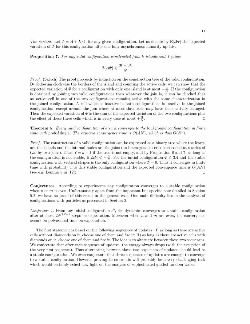
11

The variant. Let Φ = A+ E/4, for any given configuration. Let us denote by E[∆Φ] the expectedvariation of Φ for this configuration after one fully asynchronous minority update.

Proposition 7. For any valid configuration constructed from k islands with ` joins:

E[∆Φ] 63`− 3kN

.

Proof. (Sketch) The proof proceeds by induction on the construction tree of the valid configuration.By following clockwise the borders of the island and counting the active cells, we can show that theexpected variation of Φ for a configuration with only one island is at most − 3

N . If the configurationis obtained by joining two valid configurations then whatever the join is, it can be checked thatan active cell in one of the two configurations remains active with the same characterization inthe joined configuration. A cell which is inactive in both configurations is inactive in the joinedconfiguration, except around the join where at most three cells may have their activity changed.Then the expected variation of Φ is the sum of the expected variation of the two configurations plusthe effect of these three cells which is in every case at most + 3

N . ut

Theorem 5. Every valid configuration of area A converges to the background configuration in finitetime with probability 1. The expected convergence time is O(AN), which is thus O(N2).

Proof. The construction of a valid configuration can be expressed as a binary tree where the leavesare the islands and the internal nodes are the joins (an heterogenous series is encoded as a series oftwo-by-two joins). Thus, ` = k − 1 if the tree is not empty, and by Proposition 6 and 7, as long asthe configuration is not stable, E[∆Φ] 6 − 3

N . For the initial configuration Φ 6 3A and the stableconfiguration with vertical stripes is the only configuration where Φ = 0. Thus it converges in finitetime with probability 1 to this stable configuration and the expected convergence time is O(AN)(see e.g. Lemma 5 in [12]). ut

Conjectures. According to experiments any configuration converges to a stable configurationwhen n or m is even. Unfortunately apart from the important but specific case detailed in Section5.2, we have no proof of this result in the general case. One main difficulty lies in the analysis ofconfigurations with particles as presented in Section 3.

Conjecture 1. From any initial configuration c0, the dynamics converges to a stable configurationafter at most 2N3N+1 steps on expectation. Moreover when n and m are even, the convergenceoccurs on polynomial time on expectation.

The first statement is based on the following sequences of updates : I) as long as there are activecells without diamonds on it, choose one of them and fire it; II) as long as there are active cells withdiamonds on it, choose one of them and fire it. The idea is to alternate between these two sequences.We conjecture that after each sequence of updates, the energy always drops (with the exception ofthe very first sequence). Thus alternating between these two sequences of updates should lead toa stable configuration. We even conjecture that three sequences of updates are enough to convergeto a stable configuration. However proving these results will probably be a very challenging taskwhich would certainly sched new light on the analysis of sophisticated guided random walks.

12

6 Conclusion

The behavior of 2D Minority with the Moore neighborhood under fully asynchronous dynamics issurprisingly rich and difficult to analyze. The approach outlined in [1] for the von Neumann neigh-borhood is useful. The analysis of the energy and of the competing regions requires however a veryaccurate comprehension of the combinatorics of the automaton, which turned out to be more com-plex for the Moore neighborhood. A key to complete the analysis seems to find the most appropriatedefinitions for particles and rails and explain precisely how they evolve. More generally, it wouldalso be interesting to investigate the link (if any) between the Moore neighborhood topology andthe raise of stripes in totalistic asynchronous cellular automata. The development of mathematicaltools to predict the dynamics of such models appears as an essential complement to simulations.

References

1. Regnault, D., Schabanel, N., Thierry, E.: Progresses in the analysis of stochastic 2D cellular automata:a study of asynchronous 2D Minority. In: Proceedings of MFCS’2007. (2007) 320–332

2. Ermentrout, G.B., Edlestein-Keshet, L.: Cellular automata approaches to biological modelling. Journalof Theoretical Biology 160 (1993) 97–133

3. Silva, H.S., Martins, M.L.: A cellular automata model for cell differentiation. Physica A: StatisticalMechanics and its Applications 322 (2003) 555–566

4. Demongeot, J., Aracena, J., Thuderoz, F., Baum, T.P., Cohen, O.: Genetic regulation networks: circuits,regulons and attractors. C.R. Biologies 326 (2003) 171–188

5. Goles, E., Martinez, S.: Neural and automata networks, dynamical behavior and applications. Volume 58of Maths and Applications. Kluwer Academic Publishers (1990)

6. Bersini, H., Detours, V.: Asynchrony induces stability in cellular automata based models. In: Proceed-ings of Artificial Life IV, Cambridge, MIT Press (1994) 382–387

7. Buvel, R., Ingerson, T.: Structure in asynchronous cellular automata. Physica D 1 (1984) 59–688. Fates, N., Morvan, M.: An experimental study of robustness to asynchronism for elementary cellular

automata. Complex Systems 16(1) (2005) 1–279. Huberman, B.A., Glance, N.: Evolutionary games and computer simulations. Proceedings of the

National Academy of Sciences, USA 90 (Aug. 1993) 7716–771810. Kanada, Y.: Asynchronous 1d cellular automata and the effects of fluctuation and randomness. In:

Proceedings of the Fourth Conference on Artificial Life (A-Life IV), MIT Press (1994)11. Schonfisch, B., de Roos, A.: Synchronous and asynchronous updating in cellular automata. BioSystems

51 (1999) 123–14312. Fates, N., Morvan, M., Schabanel, N., Thierry, E.: Fully asynchronous behaviour of double-quiescent

elementary cellular automata. Theoretical Computer Science 362 (2006) 1–1613. Fates, N., Regnault, D., Schabanel, N., Thierry, E.: Asynchronous behaviour of double-quiescent ele-

mentary cellular automata. In: Proceedings of LATIN’2006. Volume 3887 of LNCS., Springer (2006)14. Fuks, H.: Non-deterministic density classification with diffusive probabilistic cellular automata. Phys.

Rev. E 66(2) (2002)15. Fuks, H.: Probabilistic cellular automata with conserved quantities. Nonlinearity 17(1) (2004) 159–17316. Balister, P., Bollobas, B., Kozma, R.: Large deviations for mean fields models of probabilistic cellular

automata. Random Structures & Algorithms 29 (2006) 399–41517. McCoy, B., Wu, T.T.: The Two-Dimensional Ising Model. Harvard University Press (1974)18. Rojas, R.: Neural Networks: A Systematic Introduction. Springer (1996) Chap. 13 - The Hopfield

Model.19. Fates, N., Morvan, M.: Perturbing the topology of the game of life increases its robustness to asynchrony.

In: LNCS Proc. of 6th Int. Conf. on Cellular Automata for Research and Industry (ACRI 2004). Volume3305. (Oct. 2004) 111–120