On Statistical Inferencesvia

Convex Optimization

A. NemirovskiGeorgia Institute of Technology

joint research with

Anatoli JuditskyUniversite Grenoble Alpes

Workshop on the Interface of Statistics and OptimizationThe Statistical and Applied Mathematical Sciences

InstituteFebruary 7, 2017

♣ Fact: Many inference procedures in Statistics reduce tooptimization♠ Example: MLE – Maximum Likelihood Estimation

Problem: Given a parametric family pθ(·) : θ ∈ Θof probability densities on Rd and a random observa-tion ω drawn from some density pθ?(·) from the family,estimate the parameter θ?.Maximum Likelihood Estimate: Given ω, maximizepθ(ω) over θ ∈ Θ and use the maximizer θ = θ(ω)

as an estimate of θ?.

Note: In MLE, optimization is used for number crunching onlyand has nothing to do with motivation and performance anal-ysis of MLE.

♣ Most of traditional applications of Optimization in Statisticsare of “number crunching” nature.• In contrast, we will focus on inference routines motivated andjustified by Optimization Theory – Convex Analysis, OptimalityConditions, Duality...

1

Detector-Based Hypothesis TestingDetectors & Detector-Based Pairwise Tests

♣ Situation: Given two families P1, P2 of probability distribu-tions on an observation space Ω and an observation ω ∼ P

with P known to belong to P1∪P2, we want to decide whetherP ∈ P1 (hypothesis H1) or P ∈ P2 (hypothesis H2).♣ Detectors. A detector is a function φ : Ω → R. Risks of adetector φ w.r.t. P1,P2 are defined as

Risk1(φ|P1,P2) = supP∈P1

∫Ω

e−φ(ω)P (dω),

Risk2(φ|P1,P2) = supP∈P2

∫Ω

eφ(ω)P (dω)

Risk1(φ|P1,P2) = Risk2(−φ|P2,P1)

♠ Simple test Tφ associated with detector φ, given observa-tion ω,• accepts H1 – Tφ(ω) = 1 – when φ(ω) ≥ 0,• accepts H2 – Tφ(ω) = 2 – when φ(ω) < 0.♣ Immediate observation:

Risk1[Tφ|H1, H2] ≤ Risk1(φ|P1,P2)Risk2[Tφ|H1, H2] ≤ Risk2(φ|P1,P2)

(∗)

where test’s risks Risk1, Risk2 are

Riskχ[Tφ|H1, H2] = supP∈Pχ

Probω∼PTφ(ω) 6= χ

Reason for (∗): Probω∼P ω : ψ(ω) ≥ 0 ≤

∫eψ(ω)P (dω).

2

Risk1(φ|P1,P2) = supP∈P1

∫Ω

e−φ(ω)P (dω),

Risk2(φ|P1,P2) = supP∈P2

∫Ω

eφ(ω)P (dω)

♣ Detectors admit simple “calculus:”

♣ Renormalization: φ(·)⇒ φa(·) = φ(·)− a

⇒

Risk1(φa|P1,P2) = eaRisk1(φ|P1,P2)Risk2(φa|P1,P2) = e−aRisk2(φ|P1,P2)

⇒What matters, is the product

[Risk(φ|P1,P2)]2 := Risk1(φ|P1,P2)Risk2(φ|P1,P2)

of partial risks of a detector. Shifting the detector by constant,we can distribute this product between factors as we want,e.g., always can make the detector balanced:

Risk(φ|P1,P2) = Risk1(φ|P1,P2) = Risk2(φ|P1,P2).

3

♣ Passing to multiple observations. For 1 ≤ k ≤ K, let• P1,k,P2,k be families of probability distributions on obser-

vation spaces Ωk,• φk be detectors on Ωk.♥ Families P1,k,P2,kKk=1 give rise to families of productdistributions on ΩK = Ω1 × ...×ΩK :

PKχ = PK = P1 × ...× PK : Pk ∈ Pχ,k, 1 ≤ k ≤ K, χ = 1,2,

and detectors φ1, .., φK give rise to detector φK on ΩK :

φK(ω1, ..., ωK︸ ︷︷ ︸ωK

) =K∑k=1

φk(ωk).

♠ Observation: We have

Riskχ(φK|PK1 ,PK2 ) =

K∏k=1

Riskχ(φk|P1,k,P2,k).

4

♣ From pairwise detectors to detectors for unionsAssume that we are given an observation space Ω along with• R families Rr, r = 1, ..., R of “red” probability distribu-

tions on Ω,• B families Bb, b = 1, ..., B of “brown” probability distribu-

tions on Ω,• pairwise detectors φrb(·), 1 ≤ r ≤ R, 1 ≤ b ≤ B.

εrb := Risk(φrb|Rr,Bb) = Risk1(φrb|Rr,Bb) = Risk2(φrb|Rr,Bb),

Let us aggregate the red and the brown families as follows

R =R⋃r=1

Rr, B =B⋃b=1

Bb

and consider matrices

E =

ε1,1 · · · ε1,B... · · · ...

εR,1 · · · εR,B

, F =

[E

ET

]The maximal eigenvalue of F is the spectral norm ‖E‖2,2 ofE, and the leading eigenvector [g; f ] can be selected to bepositive, giving rise to shifted detectors

ψrb(ω) = φrb(ω)− ln(fb/gr)

which can further be assembled into the detector

ψ(ω) = maxr≤R

minb≤B

ψrb(ω)

Theorem: Partial risks of detector ψ on aggregated familiesR, B are ≤ ‖E‖2,2.

5

Detector-Based Tests ”Up to Closeness”

♣ Situation: We are given L families of probability distribu-tions P`, 1 ≤ ` ≤ L, on observation space Ω, and observea realization of random variable ω ∼ P taking values in Ω.Given ω, we want to decide on the L hypotheses

H` : P ∈ P`, 1 ≤ ` ≤ L.

Our ideal goal would be to find a low-risk simple test decidingon the hypotheses.However: It may happen that the “ ideal goal” is not achiev-able, for example, when some pairs of families P` havenonempty intersections. When P` ∩ P`′ 6= ∅ for some ` 6= `′,there is no way to decide on the hypotheses with risk < 1/2.But: Impossibility to decide reliably on all L hypotheses “indi-vidually” does not mean that no meaningful inferences can bedone.

6

♠ Example: Consider 3 colored rectangles on the plane:

and 3 hypotheses, with H`, 1 ≤ ` ≤ 3, stating that our obser-vation is ω = x + ξ with deterministic “signal” x belonging to`-th rectangle and ξ ∼ N (0, σ2I2).♥ Whatever small σ be, no test can decide on the 3 hypothe-ses with risk < 1/2; e.g., there is no way to decide reliably onH1 vs. H2.However, we may hope that when σ is small, we can discardreliably some of the hypotheses. For example, if the actualsignal is brown, we cannot exclude the possibility for it to beclaimed green, but hopefully can infer that it is not blue.

♠ When handling multiple hypotheses which cannot be re-liably decided upon “as they are,” it makes sense to speakabout testing the hypotheses “up to closeness.”

7

♠ Situation: We are given• L families of probability distributions P`, ` = 1, ..., L, on

observation space Ω, giving rise to L hypotheses H`, on thedistribution P of random observation ωinΩ:

H` : P ∈ P`, 1 ≤ ` ≤ L;

• closeness relation C – a set C of pairs (`, `′) of indexes of“close to each other” hypotheses H`, H`′ such that (`, `) ∈ C(every hypothesis is close to itself) and (`, `′) ∈ C whenever(`′, `) ∈ C (closeness is symmetric).• system of balanced detectors

φ``′ : ` < `′, (`, `′) 6∈ C

along with upper bounds ε``′ on detectors’ risks:

∀(`, `′ : ` < `′, (`, `′) 6∈ C) :

∫Ω e−φ``′(ω)P (dω) ≤ ε``′ ∀P ∈ P`∫Ω eφ``′(ω)P (dω) ≤ ε``′ ∀P ∈ P`′

• Our goal is to build single-observation test deciding on hy-potheses H1, ..., HL up to closeness C.♠ Definition. Let T be a test which, given observation ω, ac-cepts some of the hypotheses H` and rejects the remaininghypotheses. We say that C-risk of T is ≤ ε, if, whenever thedistribution P of the observation obeys H`∗ for some `∗ ≤ L,the P -probability of the event “H`∗ is accepted, and all ac-cepted hypotheses are C-close to H`∗” is at least 1− ε.

8

♠ Proposition. The pairwise detectors φ``′ can be straight-forwardly assembled into single-observation test T with C-riskupper-bounded by∥∥∥[ε``′χ``′]L`,`′=1

∥∥∥2,2

[χ``′ =

1, (`, `′) 6∈ C0, (`, `′) ∈ C

],

♠ Corollary. Let ε``′ ≤ θ < 1 whenever (`, `′) 6∈ C and letstationary K-repeated observations – i.i.d. samples

ωK = (ω1, ..., ωK)

drawn from distributions in question – be allowed. Then theK-repeated version T K of T – with detectors

φ(K)``′ (ωK) =

∑Kt=1 φ``′(ωt)

in the role of φ``′ – satisfies

RiskC[T K|H1, ..., HL] ≤ θKL.

9

♣ “Universality” of detector-based tests. Let Pχ, χ =

1,2, be two families of probability distributions on observa-tion space Ω,and Hχ, χ = 1,2, be associate hypotheses onthe distribution of an observation.

Assume that there exists a simple deterministic or random-ized test T deciding onH1,H2 with risk≤ ε ∈ (0,1/2). Thenthere exists a detector φ with

Risk(φ|P1,P2) ≤ ε+ := 2√ε[1− ε] < 1.

♠ Note: Risk 2√ε[1− ε] of the detector-based test induced

by simple test T is “much worse” than the risk ε of T .However: When repeated observations are allowed, we cancompensate for risk deterioration ε 7→ 2

√ε[1− ε] by pass-

ing in the detector-based test from a single observation to amoderate number of them.

10

infφ

Risk(φ|P1,P2) = min

ε :

∫Ω e−φ(ω)P (dω) ≤ ε ∀(P ∈ P1)∫

Ω eφ(ω)P (dω) ≤ ε ∀(P ∈ P2)

(!)

Note:• The optimization problem specifying risk is convex in φ, ε•When passing from families Pχ, χ = 1,2, to their convex

hulls, the risk of a detector remains intact.

♣ Intermediate conclusion: It would be nice to solve (!),thus arriving at the lowest risk detector-based tests.But: (!) is an optimization problem with infinite-dimensionaldecision “vector” and infinitely many constraints.⇒ (!) in general is intractable.

Simple observation schemes: A series of special caseswhere (!) is efficiently solvable via Convex Optimization.

11

Simple Observation Schemes

♣ Simple Observation Scheme admits a formal definitionwhich we skip.Instructive examples are as follows.

♠ Gaussian o.s.:

ω = A(x) +N (0, Id)

• A(x): affine image of unknown signal x varying in signalspace X := Rn.• Gaussian o.s. is the standard observation model in SignalProcessing.

♠ Poisson o.s.:

ω ∈ Zd, ωi ∼ Poisson[Ai(x)] independent across i = 1, ..., d

• Ai(x): affine functions of unknown signal x varying in agiven open convex signal space X ⊂ Rn such that Ai(x) >

0, x ∈ X .Poisson o.s. arises in Poisson Imaging, including• Positron Emission Tomography,• Large binocular Telescope,• Nanoscale Fluorescent Microscopy.

12

♠ Discrete o.s.:

ω ∈ e1, ..., ed takes value ei with probability Ai(x)

• ei: i-th basic orth in Rd

• Ai: affine functions of unknown signal x varying in a givenopen convex signal space X ⊂ Rn such that Ai(x) > 0 and∑iAi(x) = 1, x ∈ X .

♠ K-repeated version of a simple o.s.:

ω = ΩK := (ω1, ..., ωK)

with ωt sampled, independently across t, from observations ofan unknown signal x ∈ X yielded by a simple o.s., e.g., Gaus-sian/Poisson/Discrete one.

♠ Note: Distributions P of observations in a simple o.s. pos-sess positive continuous densities p(·) w.r.t. a properly se-lected reference measure Π on the space of observations.

♠ Convex hypothesis HX in a simple o.s. is specified bya nonempty convex compact subset X of the correspondingsignal space X and states that the signal x underlying obser-vation belongs to X.

13

ε?(P1,P2) = min

ε :

∫Ω e−φ(ω)P (dω) ≤ ε ∀(P ∈ P1)∫Ω eφ(ω)P (dω) ≤ ε ∀(P ∈ P2)

(!)

♣Main Result. For χ = 1,2, letPχ of probability distributions obeyingconvex hypothesis Hχ : x ∈ Xχ in a simple o.s. The problem

Opt = maxp1,p2

∫ √p1(ω)p2(ω)Π(dω) : pχ(·) is the density

of a distribution from Pχ, χ = 1,2

(!)

is equivalent to an explicit finite-dimensional convex program and is solv-able. Optimal solution (p∗1(·), p∗2(·)) to the problem gives rise to the mini-mum risk balanced detector

φ∗(ω) =1

2ln(p∗1(ω)/p∗2(ω))

for P1, P2. This detector is an affine function of ω, and the risk of thedetector is Opt.• In our standard o.s.’s, (!) reads:

• Gaussian o.s.: ln(Opt) = −18

minx∈X1,

y∈X2

‖A(x)−A(y)‖22

[Π: Lebesque measure]

• Poisson o.s.: ln(Opt) = −12

minx∈X1,

y∈X2

∑i[A

1/2i (x)−A1/2

i (y)]2

[Π: counting measure]

• Discrete o.s.: Opt = maxx∈X1,

y∈X2

∑iA

1/2i (x)A1/2

i (y)

[Π: counting measure]

For K-repeated version of a simple o.s., the optimal detector is

φ(K)∗ (ωK) =

K∑t=1

φ∗(ωt),

and its risk is OptK = OptK.

14

Near-Optimality of Minimum Risk Detector-Based Testsin Simple Observation Schemes

♣ Proposition A. Let HXχ, χ = 1,2, be convex hypothesesin a simple o.s., and Pχ be the family of distributions obeyingthe hypotheses. Assume that in the nature there exists a sim-ple single-observation test T , deterministic or randomized, Twith

Risk[T |H1, H2] ≤ ε < 1/2.

Then the risk of the simple test Tφ∗ accepting H1 whenφ∗(ω) ≥ 0 and accepting H2 otherwise is comparable to ε:

Risk[Tφ∗|H1, H2] ≤ ε+ := 2√ε(1− ε) < 1.

15

♣ Proposition B. Let Hχ, χ = 1,2, be convex hypotheses ina simple o.s. Assume that for some ε < 1/2 and K∗ in the na-ture there exists a test, based on K∗-repeated observations,with risk ≤ ε. Then the risk of the test T

φ(K)∗

with

K ≥ K∗ = 2

[ln(1/ε)

ln(1/ε)− ln(4(1− ε))

]︸ ︷︷ ︸

→1 as ε→+0

K∗.

does not exceed ε as well.

♣ Proposition C. Let H`, ` = 1,2, ..., L, be convex hypothe-ses in a simple o.s., and C be a closeness relation. Assumethat for some ε < 1/2 and K∗ in the nature there exists atest, based on K∗-repeated observations, deciding on the hy-potheses with C-risk ≤ ε. Then the efficiently computable K-observation test T K yielded by assembling optimal pairwisedetectors with

K ≥ 2

[ln(1/ε) + ln(L− 1)

ln(1/ε)− ln(4(1− ε))

]︸ ︷︷ ︸

→1 as ε→+0

K∗.

has C-risk ≤ ε as well.

16

♣Generic applications of minimum-risk-detector-based testsin simple o.s. include

• near-optimal estimation of linear/factional-linear function-als on finite unions of convex signal sets

• sequential testing of multiple convex hypotheses

• change point detection in linear dynamical systems

• rudimentary measurement design

17

Illustration: Estimating Fractional-Linear Functional onUnion of Convex Sets

♠ Situation: Signal x known to belong to the finite union

X =M⋃µ=1

Xµ

of given convex compact setsXµ is observed via a Simple o.s.Given a linear-fractional function

F (u) =aTu+ b

cTu+ d: X → R,

[minu∈X

cTu+ d > 0]

we want to recover f(x) via observation(s) associated with x.

18

♠ Strategy: Given N , we• split the range ∆ = [minx∈X F (x),maxx∈X F (x)] into

N consecutive bins ∆ν of length δN = |∆|/N ,• define MN convex hypotheses

Hµν : x ∈ Xµ & F (x) ∈∆ν

• use pairwise optimal detectors to decide on the convexhypotheses Hµν, 1 ≤ µ ≤M , 1 ≤ ν ≤ N up to closeness

C : Hµν is close to Hµ′ν′ ⇔∆ν ∩∆ν′ 6= ∅• estimate F (x) by the center of masses F of the union of

bins ∆ν associated with the accepted hypotheses Hµν.♠ Fact: For the resulting test T the recovery error does notexceed δN with probability at least 1−RiskC[T |H1,1, ..., HM,N ].♠ Near-Optimality: Let ε ∈ (0,1/2). Assume in the naturethere exists an estimator recovering F (x), x ∈ X, (1 − ε)-reliably within accuracy δN/2 via K∗ observations. ThenProb|F − F (x)| > δN ≤ ε, provided that the number K ofobservations underlying F satisfies

K ≥ 2

[ln(MN/ε)

ln(1/ε)− ln(4(1− ε))

]K∗.

19

♣ Observation: A “common denominator” of minimum riskdetectors for simple o.s.’s is their affinity in observations.

♠ Fact: Presumably good affine detectors can be found, ina computationally efficient way, in many important situationswhich are beyond simple o.s.’s.

20

Setup

♣ Given an observation space Ω = Rd, consider a tripleH,M,Φ, where• H is a nonempty closed convex set in Ω symmetric w.r.t.

the origin,• M is a closed convex set in some Rn,•Φ(h;µ) : H×M→ R is a continuous function convex in

h ∈ H and concave in µ ∈M.

♣ H,M,Φ specify a family S[H,M,Φ] of probability distri-butions on Ω. A probability distribution P belongs to the familyiff there exists µ ∈M such that

ln(∫

Ωeh

TωP (dω))≤ Φ(h;µ) ∀h ∈ H (∗)

We refer to µ ensuring (∗) as to parameter of distribution P .• Warning: A distribution P may have many different param-eters!♥ We refer to triple H,M,Φ satisfying the above require-ments as to regular data, and to S[H,M,Φ] – as to the sim-ple family of distributions induced by these data.

21

♠ Example 1: Gaussian and sub-Gaussian distributions.When M = (u,Θ) ⊂ Rd × intSd+ is a convex compactset such that Θ 0 for all (u,Θ) ∈ M, H = Rd andΦ(h;u,Θ) = hTu + 1

2hTΘh, S = S[H,M,Φ] contains

all probability distributions P which are sub-Gaussian with pa-rameters (u,Θ), meaning that

ln(∫

Ωeh

TωP (dω))≤ hTu+

1

2hTΘh ∀h, (1)

and, in addition, the “parameter” (u,Θ) belongs toM.Note: Whenever P is sub-Gaussian with parameters (u,Θ),u is the expectation of P .

Note: N (u,Θ) ∈ S whenever (u,Θ) ∈ M; for P =

N (u,Θ), (1) is an identity.♠ Example 2: Poisson distributions. WhenM ⊂ Rd+ is aconvex compact set, H = Rd and

Φ(h;µ) =d∑

i=1

µi(ehi − 1),

S = S[H,M,Φ] contains distributions of all d-dimensionalrandom vectors ωi with independent across i entries ωi ∼Poisson(µi) such that µ = [µ1; ...;µd] ∈M.

22

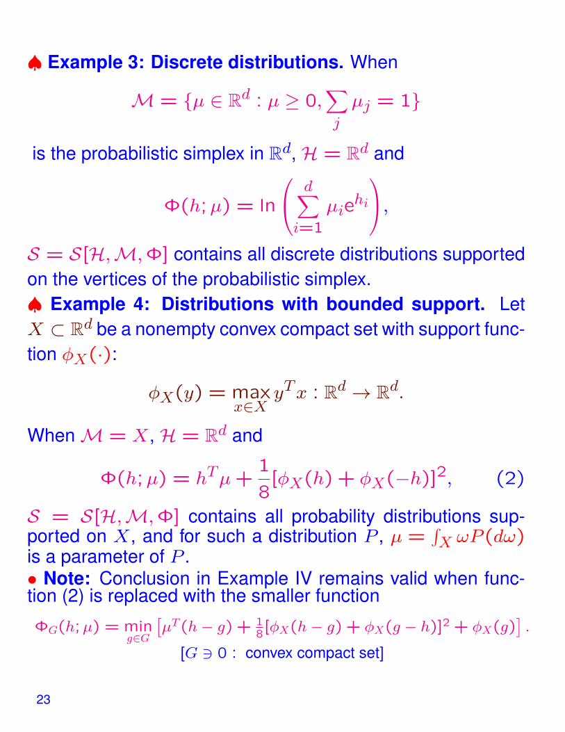
♠ Example 3: Discrete distributions. When

M = µ ∈ Rd : µ ≥ 0,∑j

µj = 1

is the probabilistic simplex in Rd, H = Rd and

Φ(h;µ) = ln

d∑i=1

µiehi

,S = S[H,M,Φ] contains all discrete distributions supportedon the vertices of the probabilistic simplex.♠ Example 4: Distributions with bounded support. LetX ⊂ Rd be a nonempty convex compact set with support func-tion φX(·):

φX(y) = maxx∈X

yTx : Rd → Rd.

WhenM = X, H = Rd and

Φ(h;µ) = hTµ+1

8[φX(h) + φX(−h)]2, (2)

S = S[H,M,Φ] contains all probability distributions sup-ported on X, and for such a distribution P , µ =

∫X ωP (dω)

is a parameter of P .• Note: Conclusion in Example IV remains valid when func-tion (2) is replaced with the smaller function

ΦG(h;µ) = ming∈G

[µT(h− g) + 1

8[φX(h− g) + φX(g − h)]2 + φX(g)

].

[G 3 0 : convex compact set]

23

♣ Main observation: When deciding on simple families ofdistributions, affine tests and their risks can be efficiently com-puted via Convex Programming:♥ Theorem. Let Hχ,Mχ,Φχ, χ = 1,2, be two collectionsof regular data with common H1 = H2 =: H, and let

Ψ(h) = maxµ1∈M1,µ2∈M2

1

2[Φ1(−h;µ1) + Φ2(h, µ2)]︸ ︷︷ ︸

Φ(h;µ1,µ2)

: H → R

Then Ψ is efficiently computable continuous convex function,and for every h ∈ H, setting

φ(ω) = hTω +1

2

[maxµ1∈M1

Φ1(−h;µ1)− maxµ2∈M2

Φ1(h;µ2)

]︸ ︷︷ ︸

κ

,

one has

Risk(φ|P1,P2) ≤ expΨ(h) [Pχ = S[H,Mχ,Φχ]]

In particular, if convex-concave function Φ(h;µ1, µ2) pos-sesses a saddle point h∗, (µ∗1, µ

∗2) on H× (M1 ×M2), the

affine detector

φ∗(ω) = hT∗ ω +1

2

[Φ1(−h;µ∗1)−Φ2(h∗;µ∗2)

]admits risk bound

Risk(φ|P1,P2) ≤ expΦ(h∗;µ∗1, µ2)

24

♣ Example: Sub-Gaussian Direct Product case. For χ =

1,2, let Uχ ⊂ Ω = Rd and Vχ ⊂ intSd+ be convex compactsets. Setting

Mχ = Uχ × Vχ, Φ(h;u,Θ) = hTu+1

2hTΘh : H×Mχ → R,

the regular data H = Rd,Mχ,Φ specify the families

Pχ = S[Rd, Uχ × Vχ,Φ]

of sub-Gaussian distributions with parameters from Uχ × Vχ.

♠ Saddle point problem responsible for the design of affinedetector for P1,P2 reads

SadVal = minh∈Rd

maxu1∈U1,u2∈U2

Θ1∈V1,Θ2∈V2

1

2

[hT(u2 − u1) +

1

2hT [Θ1 + Θ2]h

]The problem is efficiently solvable, and its solution yields affinedetector φ∗ with risk

Risk(φ∗|P1,P2) ≤ expSadVal.

♥ Note: In the symmetric case V1 = V2 the affine detectorwe end up with is the minimum risk detector for P1, P2.

25

♠ Beyond Direct Product case: Let

Qχ = (µ,Θ) ∈ Rd × Sd++, χ = 1,2[Sd++ = Θ ∈ Sd : Θ 0

]be convex compact sets. Applying Theorem, we can test thehypotheses

Hχ : ω ∼ N (µ,Θ) with (µ,Θ) ∈ Qχ, χ = 1,2

via affine detector readily given by the solution to an explicitconvex-concave saddle point problem.

Note: Utilizing sets Qχ, we extend Gaussian o.s. by allowingfor dependencies between the mean and the covariance ofobservations.

26

What is “affine?” Quadratic Lifting

♣ We have developed a technique for building reasonableaffine detectors for simple families of distributions.But: Given observation ζ ∼ P , we can subject it to nonlineartransformation ζ 7→ ω = ψ(ζ), e.g., quadratic lifting

ζ 7→ ω = (ζ, ζζT )

and treat as our observation ω rather than the “true” observa-tion ζ. Affine in ω detectors are nonlinear in ζ.Example: Detectors affine in the quadratic lifting ω =

(ζ, ζζT ) of ζ are exactly the quadratic functions of ζ.♠ We can try to apply our machinery for building affine de-tectors to nonlinear transformations of true observations, thusarriving at nonlinear detectors.• Bottleneck: To apply the outlined strategy to a pair P1,P2

of families of distributions of interest, we need to cover thefamilies P+

χ of distributions of ω = ψ(ζ) induced by distribu-tions P ∈ Pχ, χ = 1,2, by simple families of distributions.

♠ The bottleneck can be resolved reasonably well for Gaus-sian and sub-Gaussian distributions.

27

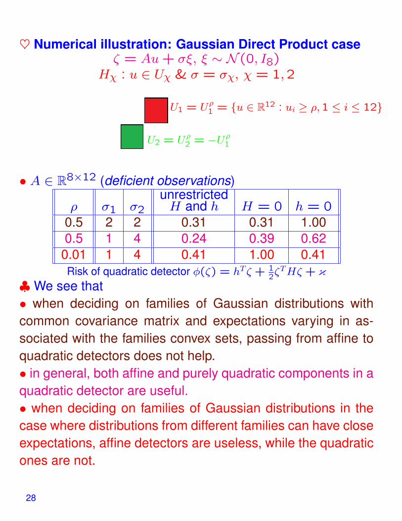
♥ Numerical illustration: Gaussian Direct Product caseζ = Au+ σξ, ξ ∼ N (0, I8)

Hχ : u ∈ Uχ & σ = σχ, χ = 1,2

U1 = Uρ1 = u ∈ R12 : ui ≥ ρ,1 ≤ i ≤ 12

U2 = Uρ2 = −Uρ

1

• A ∈ R8×12 (deficient observations)

ρ σ1 σ2unrestrictedH and h H = 0 h = 0

0.5 2 2 0.31 0.31 1.000.5 1 4 0.24 0.39 0.62

0.01 1 4 0.41 1.00 0.41Risk of quadratic detector φ(ζ) = hTζ + 1

2ζTHζ + κ

♣We see that• when deciding on families of Gaussian distributions withcommon covariance matrix and expectations varying in as-sociated with the families convex sets, passing from affine toquadratic detectors does not help.• in general, both affine and purely quadratic components in aquadratic detector are useful.• when deciding on families of Gaussian distributions in thecase where distributions from different families can have closeexpectations, affine detectors are useless, while the quadraticones are not.

28

♣ Model: We observe one by one vectors (“vectorized” 2Dimages)

ωt = xt + ξt,

• xt: deterministic image• ξt ∼ N (0, σ2Id): independent across observation noises.Note: We know a range [σ, σ] of σ, but perhaps do notknow σ exactly.

• We know that x1 = x2 and want to check whether x1 =

... = xK (“no change”) or there is a change.♠ Goal: Given an upper bound ε > 0 on the probability offalse alarm, we want to design a sequential change detectionroutine capable to detect change, if any.

♠ Approach:• Pass from observations ωt, 1 ≤ t ≤ K, to observations

ζt = ωt − ω1 = xt − x1︸ ︷︷ ︸yt

+ ξt − ξ1︸ ︷︷ ︸ηt

, 2 ≤ t ≤ K

• Test null hypothesis H0 “no change” (y2 = ... = yK = 0)

vs. alternativeK⋃k=2Hρ

k : change at time k of magnitude ≥ ρ

Hρk : y2 = ... = yk−1 = 0, ‖yk‖2 ≥ ρ

via our machinery for testing multiple hypotheses Gρk onquadratic lifts Yk = yky

Tk of observations yk:

G1 : Y1 = .... = YK = 0,Gρk : Y1 = ... = Yk−1 = 0,Tr(Yk) ≥ ρ2, Yt 0 ∀t, 2 ≤ k ≤ K

up to closenessC: all brown hypotheses are close to each other and are not close

to the magenta hypothesis

• Find the smallest ρ for which the C-risk of the resulting infer-ence is ≤ ε, and utilize this inference in change point detec-tion.

30

How It Works

♠ Setup: dim y = 2562 = 65536, σ = 10, σ2/σ2 = 2,K = 9, ε = 0.01

♠ Inference: At time t = 2, ...,K, compute

φ∗(ζt) = −2.7138‖ζt‖22105

+ 366.9548.

φ∗(ζt) < 0⇒ conclude that the change took place and terminateφ∗(ζt) ≥ 0⇒ conclude that there was no change so far and proceed

to the next image, if any♠ Note:• When G1 holds true, the probability not to claim change

on time horizon 1, ...,K is at least 0.99.• When Gρk holds true, the change at time ≤ k is detected

with probability at least 0.99, provided ρ ≥ ρ∗ = 2716.6 (av-erage per pixel energy in yk at least by 12% larger than σ2)• No test can 0.99-reliably decide via ζ1, ..., ζk on Gρk vs. G1,

provided ρ/ρ∗ < 0.965.• In the movie, the change takes place at time 3 and is de-

tected at time 4.

31

Signal Estimation in Gaussian O.S.

♣ Situation: “In the nature” there exists a signal x known tobelong to a given convex compact set X ⊂ Rn. We observecorrupted by noise affine image of the signal:

ω = Ax+ σξ ∈ Rm

•A: given m× n sensing matrix•ξ: random observation noise♠ Goal: To recover the image Bx of x under a given linearmapping•B: given k × n matrix.♠ Risk of a candidate estimate x(·) : Ω→ Rk is defined as

Risk[x|X ] = supx∈X

√Eξ

‖Bx− x(Ax+ σξ)‖22

⇒ Risk2 is the worst-case, over x ∈ X , expected ‖ ·‖22 recov-ery error.♣ Agenda: Under appropriate assumptions on X , we shallshow that• One can build, in a computationally efficient fashion, the

(nearly) best, in terms of risk, in the family of linear estimates

x(ω) = xH(ω) = HTω [H ∈ Rm×k]

• The resulting linear estimate is nearly optimal among allestimates, linear and nonlinear alike.

32

♣ Assumption on noise: ξ is zero mean with unit covariancematrix.⇒ The risk of a linear estimate xH(ω) = HTω is given by

Risk2[xH|X ] = σ2Tr(HTH) + maxx∈X

Tr([B −HTA]xxT [BT −ATH])︸ ︷︷ ︸Ψ(H)

.

♥ Note: Ψ is convex ⇒ building the minimum risk linearestimate reduces to solving convex minimization problem

Opt∗ = minH

[Ψ(H) + σ2Tr(HTH)

]. (∗)

But: Convex function Ψ is given implicitly and can be difficultto compute, making (∗) difficult as well.Fact: Basically, the only cases when (∗) is known to be easyare those when• X is given as a convex hull of finite set of moderate cardi-

nality• X is an ellipsoid.X is a box⇒ computing Ψ is NP-hard...

33

minH

σ2Tr(HTH) + max

x∈XTr([B −HTA]xxT [BT −ATH])︸ ︷︷ ︸

Ψ(H)

(∗)

♠ When Ψ is difficult to compute, we can to replace Ψ inthe design problem (∗) with an efficiently computable convexupper bound Ψ+(H).We are about to consider a family of sets X – ellitopes – forwhich reasonably tight bounds Ψ+ are available.♣ An ellitope is a bounded set X ⊂ Rn given as

X = x ∈ Rn : ∃y ∈ RN , t ∈ T : x = Ry, yTSky tk, 1 ≤ k ≤ K

where• R is a given n×N matrix,• Sk are positive semidefinite matrices• T is a convex compact subset of RK+ containing a positive

vector and monotone:

0 ≤ t′ ≤ t ∈ T ⇒ t′ ∈ T .

♠ Note: Every ellitope is a symmetric w.r.t. the origin convexcompact set.

34

♠ Basic examples:A. Intersection

⋂ix : ‖Aix‖2 ≤ 1 of finitely many

ellipsoids/elliptic cylinders centered at the originB. Intersection

⋂ix : ‖Aix‖pi ≤ 1 of finitely many

“`p balls/cylinders” centered at the origin, with 2 ≤ pi ≤ ∞♣ Note: What follows straightforwardly extends from ellitopesto their “matrix analogies” – spectratopes

X = x ∈ Rn : ∃(y ∈ RN , t ∈ T ) : x = Ry, S2k [y] tkIdk, k ≤ K

[Sk[y] : symmetric dk × dk matrices linearly depending on y]

Every ellitope is a spectratope, but not vice versa; e.g., thematrix box y ∈ Rm×n : spectral norm of y is ≤ 1 is a spec-tratope, but not an ellitope.

♠ Ellitopes/spectratopes admit fully algorithmic calculus:if Xi, 1 ≤ i ≤ I, are ellitopes/spectratopes, so are•⋂iXi

• X1 × ...×XI• Conv(

⋃iXi)

• X1 + ...+ XI• linear images of Xi• inverse linear images of Xi under linear embeddings

35

♣ Observation: It is easy to upper-bound the maximum of aquadratic form xTQx over an ellitope

X = x : ∃(t ∈ T , y) : x = Ry, yTSky ≤ tk, 1 ≤ k ≤ K.

Specifically, whenever λ ≥ 0 satisfies

RTQR ∑k

λkSk,

we have

maxx∈X

xTQx ≤ φT (λ) := maxt∈T

λT t.

36

♠ Corollary: Given an ellitope X and matricesA,B, considerthe convex optimization problem

Opt = minλ≥0,H

φT (λ) + σ2Tr(HTH) :

[ ∑kλkSk BT −ATH

B −HTA I

] 0

The efficiently computable optimal solution (λ∗, H∗) to thisproblem gives rise to the linear estimate

xH∗(ω) = HT∗ ω

with risk not exceeding√

Opt. This estimate is near-optimalamong all linear estimates:

Risk[xH∗|X ] ≤ 2√

ln(5K) · infH

Risk[xH |X ]

[xH(ω) = HTω]

♠ Surprising fact: The linear estimate xH∗ is nearly optimalamong all estimates, linear and nonlinear alike.

37

♣ Theorem. Let us associate with ellitope

X = x : ∃(t ∈ T , y) : x = Ry, yTSky ≤ tk, k ≤ K

the convex compact set

Q = Q ∈ SN : Q 0, ∃t ∈ T : Tr(SkQ) ≤ tk, k ≤ K,and the quantity

M∗ = maxQ∈Q

√Tr(BRQRTBT).

The linear estimate xH∗(ω) of Bx, x ∈ X , via observationω = Ax+ σξ, ξ ∼ N (0, Im), given by the optimal solution tothe convex optimization problem

Opt = minλ≥0,H

φT (λ) + σ2Tr(HTH) :

[ ∑kλkSk BT −ATH

B −HTA I

] 0

satisfies the risk bound

Risk[xH∗|X ] ≤√

Opt ≤

√√√√6 ln

(8M2

∗K

Risk2opt[X ]

)Riskopt[X ],

where

Riskopt[X ] = infx(·)

supx∈X

√Eξ∼N (0,Im)

‖Bx− x(Ax+ σξ)‖2

2

,

inf being taken with respect to all, linear and nonlinear alike,estimates x(·), is the optimal minimax risk.

38

♠ Explanation, Easy part: Consider the parametric convexoptimization problem

Opt(ρ) = maxQ0,t∈T

Tr(B[Q−QAT(σ2I +AQAT)−1AQ

]BT)

:

Tr(SkQ) ≤ ρtk, k ≤ K

♥ Objective: Optimal expected ‖·‖22-risk of recoveryBη fromobservationAη+σξ with ξ ∼ N (0, I) independent of randomGaussian signal η ∼ N (0, Q).♥ Constraints ensure that the probability for η ∼ N (0, Q)

not to belong to X goes to 0 exponentially fast (as Ke− 1

3ρ) asρ→ +0

⇒ Minimax optimal risk Riskopt[X ] can be lower-bounded interms of Opt(·)♠ Explanation, Miracle part: By conic duality, Opt(1) turnsout to be exactly the upper bound Opt on the squared riskof the near-optimal linear estimate, and by trivial reasonsOpt(ρ) ≥ ρOpt(1)

⇒ Minimax optimal risk Riskopt[X ] can be lower-bounded interms of Opt and thus - in terms of the risk of the near-optimallinear estimate.

39