Chapter 3 Making Statistical Inferences

Chapter 3

Making Statistical Inferences

3.7 The t Distribution

3.8 Hypothesis Testing

3.9 Testing Hypotheses About Single Means

Limitations of the Normal Distribution

But, except in classroom exercises, researchers will

never actually know a population’s variance. Hence,

they can calculate neither the sampling distribution’s

standard error nor the Z score for any sample mean!

Researchers want to apply the central limit theorem to

make inferences about population parameters, using one

sample’s descriptive statistics, by applying the theoretical

standard normal distribution (Z table).

So, have we hit a statistical dead-end? ______

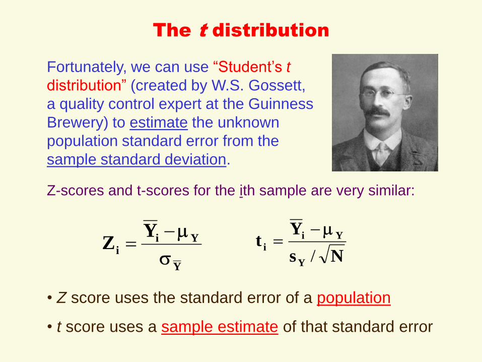
The t distribution

Z-scores and t-scores for the ith sample are very similar:

Fortunately, we can use “Student’s t

distribution” (created by W.S. Gossett,

a quality control expert at the Guinness

Brewery) to estimate the unknown

population standard error from the

sample standard deviation.

Y

Yii

YZ

Ns

Yt

Y

Yi

i/

• Z score uses the standard error of a population

• t score uses a sample estimate of that standard error

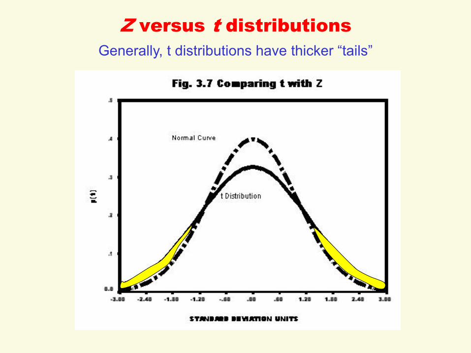
Z versus t distributions

Generally, t distributions have thicker “tails”

A Family of t distributions

The thickness of the tails depends on the sample size (N).

Instead of just one t distribution, an entire family of t

scores exists, with a different curve for every sample size

from N = 1 to .

Appendix D gives t family’s critical values

But, for large samples (N > 100), the Z and t tables have

nearly identical critical values.

(Both tables’ values are identical for N = )

Therefore, to make statistical inferences using large

samples – such as the 2008 GSS (N = 2,023 cases) –

we can apply the standard normal table to find t values!

Hypothesis Testing

The basic statistical inference question is:

What is the probability of obtaining a sample statistic if its

population has a hypothesized parameter value?

H1: Research Hypothesis - states what you really

believe to be true about the population

H0: Null Hypothesis - states the opposite of H1; this

statement is what you expect to reject as untrue

Scientific positivism is based on the logic of falsification --

we best advance knowledge by disproving null hypotheses.

We can never prove our research hypotheses beyond all

doubts, so we may only conditionally accept them.

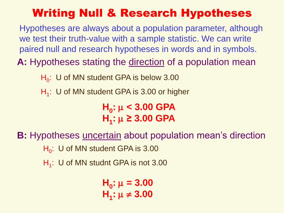
Writing Null & Research Hypotheses

Hypotheses are always about a population parameter, although

we test their truth-value with a sample statistic. We can write

paired null and research hypotheses in words and in symbols.

H0: U of MN student GPA is below 3.00

H1: U of MN student GPA is 3.00 or higher

A: Hypotheses stating the direction of a population mean

B: Hypotheses uncertain about population mean’s direction

H0: U of MN student GPA is 3.00

H1: U of MN studnt GPA is not 3.00

H0: < 3.00 GPA

H1: ≥ 3.00 GPA

H0: = 3.00

H1: 3.00

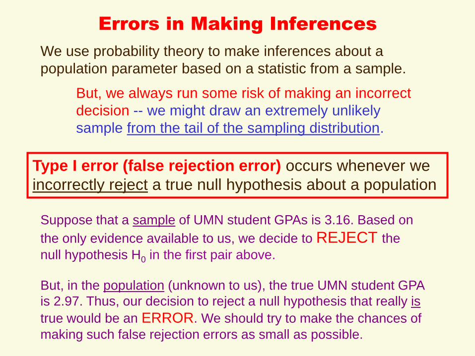
Errors in Making Inferences

We use probability theory to make inferences about a

population parameter based on a statistic from a sample.

But, we always run some risk of making an incorrect

decision -- we might draw an extremely unlikely

sample from the tail of the sampling distribution.

Type I error (false rejection error) occurs whenever we

incorrectly reject a true null hypothesis about a population

Suppose that a sample of UMN student GPAs is 3.16. Based on

the only evidence available to us, we decide to REJECT the

null hypothesis H0 in the first pair above.

But, in the population (unknown to us), the true UMN student GPA

is 2.97. Thus, our decision to reject a null hypothesis that really is

true would be an ERROR. We should try to make the chances of

making such false rejection errors as small as possible.

Type I & Type II Errors

(2) Based on the sample results,

you must decide to:

Reject null

hypothesis

Do not reject

H0

(1) In the

population

from which

that sample

came, the null

hypothesis

H0 really is:

True

False

BOX 3.2.

Correct

decision

Correct

decision

Type I or false

rejection error

()

Type II or false

acceptance

error (β)

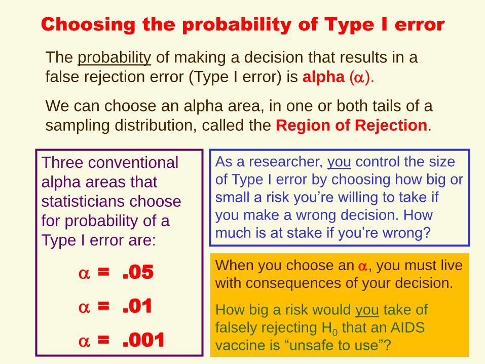
Choosing the probability of Type I error

The probability of making a decision that results in a

false rejection error (Type I error) is alpha ().

We can choose an alpha area, in one or both tails of a

sampling distribution, called the Region of Rejection.

As a researcher, you control the size

of Type I error by choosing how big or

small a risk you’re willing to take if

you make a wrong decision. How

much is at stake if you’re wrong?

Three conventional

alpha areas that

statisticians choose

for probability of a

Type I error are:

= .05

= .01

= .001

When you choose an , you must live

with consequences of your decision.

How big a risk would you take of

falsely rejecting H0 that an AIDS

vaccine is “unsafe to use”?

One- or Two-Tailed Tests?

How can you decide whether to write

a one-tailed research hypothesis --

or a two-tailed

research hypothesis?

You can use social theory, past research results, or

even your hunches to choose your hypotheses that

reflects the most likely current state of knowledge:

Two tail: states a difference, but doesn’t say where

One tail: states a clear directional difference

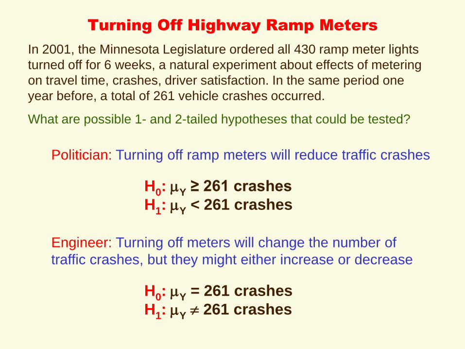
Turning Off Highway Ramp Meters

Politician: Turning off ramp meters will reduce traffic crashes

Engineer: Turning off meters will change the number of

traffic crashes, but they might either increase or decrease

H0: Y = 261 crashes

H1: Y 261 crashes

In 2001, the Minnesota Legislature ordered all 430 ramp meter lights

turned off for 6 weeks, a natural experiment about effects of metering

on travel time, crashes, driver satisfaction. In the same period one

year before, a total of 261 vehicle crashes occurred.

What are possible 1- and 2-tailed hypotheses that could be tested?

H0: Y ≥ 261 crashes

H1: Y < 261 crashes

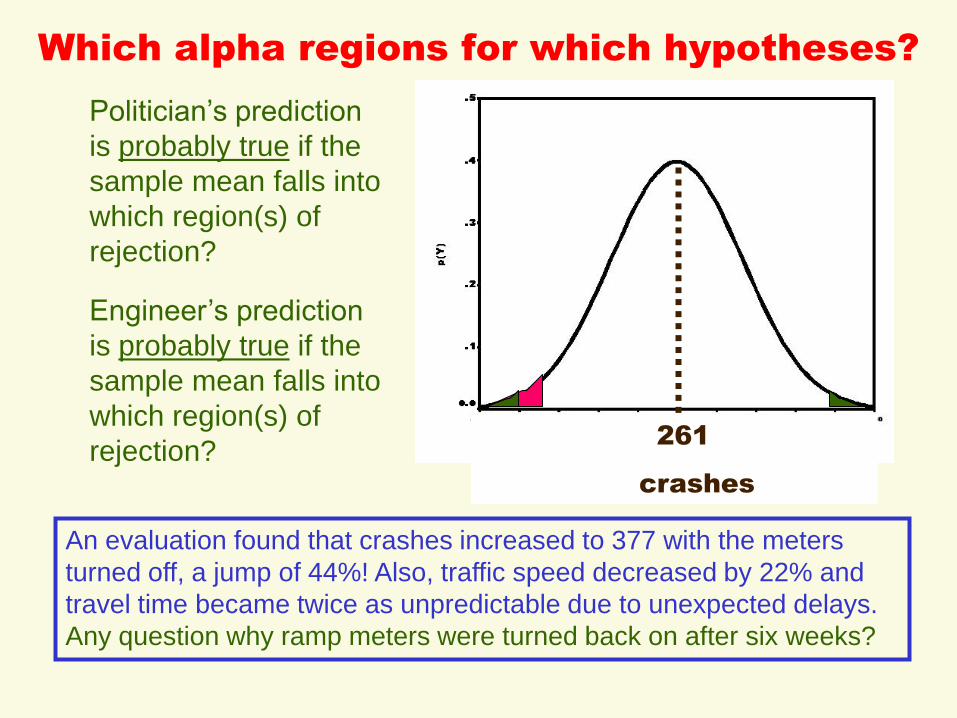
Which alpha regions for which hypotheses?

261

crashes

Politician’s prediction

is probably true if the

sample mean falls into

which region(s) of

rejection?

Engineer’s prediction

is probably true if the

sample mean falls into

which region(s) of

rejection?

An evaluation found that crashes increased to 377 with the meters

turned off, a jump of 44%! Also, traffic speed decreased by 22% and

travel time became twice as unpredictable due to unexpected delays.

Any question why ramp meters were turned back on after six weeks?

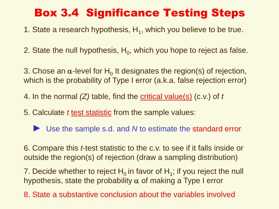
Box 3.4 Significance Testing Steps

1. State a research hypothesis, H1, which you believe to be true.

2. State the null hypothesis, H0, which you hope to reject as false.

3. Chose an -level for H0 It designates the region(s) of rejection,

which is the probability of Type I error (a.k.a. false rejection error)

4. In the normal (Z) table, find the critical value(s) (c.v.) of t

5. Calculate t test statistic from the sample values:

► Use the sample s.d. and N to estimate the standard error

6. Compare this t-test statistic to the c.v. to see if it falls inside or

outside the region(s) of rejection (draw a sampling distribution)

7. Decide whether to reject H0 in favor of H1; if you reject the null

hypothesis, state the probability of making a Type I error

8. State a substantive conclusion about the variables involved

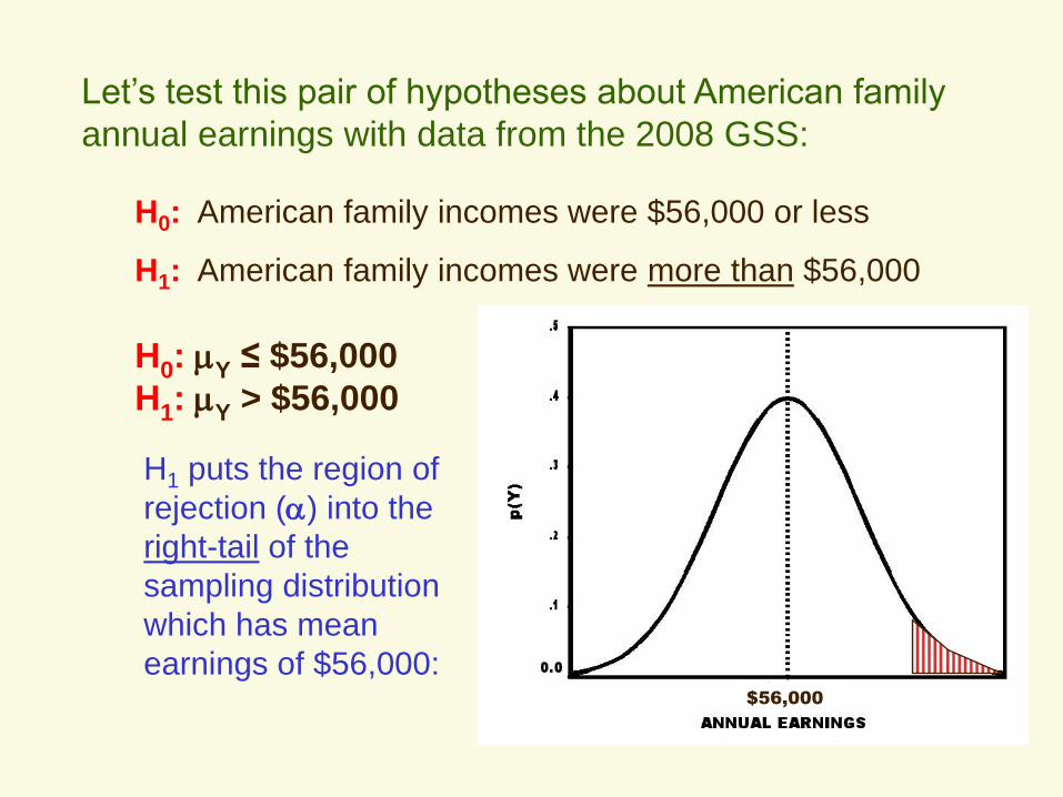
Let’s test this pair of hypotheses about American family

annual earnings with data from the 2008 GSS:

H0: American family incomes were $56,000 or less

H1: American family incomes were more than $56,000

H0: Y ≤ $56,000

H1: Y > $56,000

H1 puts the region of

rejection () into the

right-tail of the

sampling distribution

which has mean

earnings of $56,000:$56,000

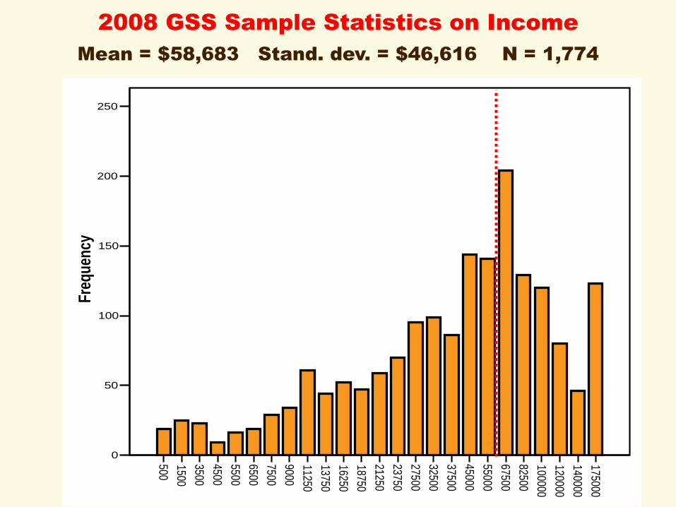
2008 GSS Sample Statistics on Income

Mean = $58,683 Stand. dev. = $46,616 N = 1,774

500

1500

3500

4500

5500

6500

7500

9000

11250

13750

16250

18750

21250

23750

27500

32500

37500

45000

55000

67500

82500

100000

120000

140000

175000

0

50

100

150

200

250

Fre

qu

ency

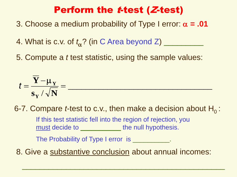
Perform the t-test (Z-test)

3. Choose a medium probability of Type I error: = .01

4. What is c.v. of t? (in C Area beyond Z) _________

5. Compute a t test statistic, using the sample values:

6-7. Compare t-test to c.v., then make a decision about H0 :

_________________________________/

Ns

Y

Y

Yt

If this test statistic fell into the region of rejection, you

must decide to ___________ the null hypothesis.

The Probability of Type I error is __________.

8. Give a substantive conclusion about annual incomes:

______________________________________________

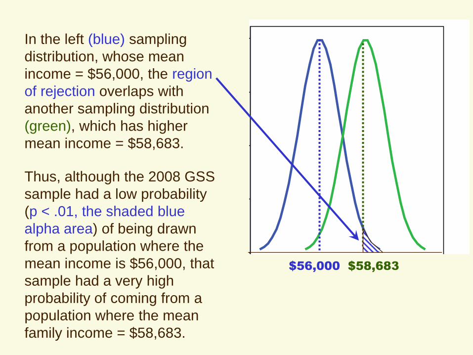
In the left (blue) sampling

distribution, whose mean

income = $56,000, the region

of rejection overlaps with

another sampling distribution

(green), which has higher

mean income = $58,683.

34.6

7

35.0

0

35.3

3

35.6

7

36.0

0

36.3

3

36.6

7

37.0

0

37.3

3

37.6

7

38.0

0

38.3

3

38.6

7

39.0

0

39.3

3

39.6

7

40.0

0

40.3

3

40.6

7

41.0

0

41.3

3

Mis

sin

g

Income ($000)

0.00

0.10

0.20

0.30

0.40

Thus, although the 2008 GSS

sample had a low probability

(p < .01, the shaded blue

alpha area) of being drawn

from a population where the

mean income is $56,000, that

sample had a very high

probability of coming from a

population where the mean

family income = $58,683.

$56,000 $58,683

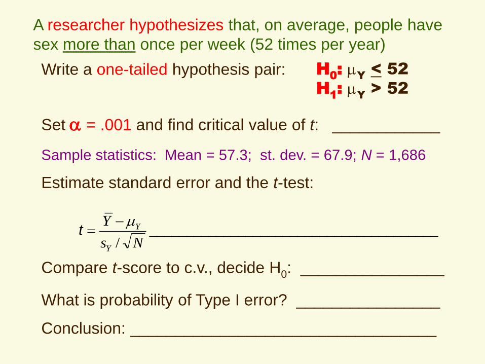
A researcher hypothesizes that, on average, people have

sex more than once per week (52 times per year)

Sample statistics: Mean = 57.3; st. dev. = 67.9; N = 1,686

Write a one-tailed hypothesis pair: H0:

Y< 52

H1:

Y> 52

Set = .001 and find critical value of t: ____________

Estimate standard error and the t-test:

_______________________________________/ Ns

Y

Y

Yt

Compare t-score to c.v., decide H0: ________________

What is probability of Type I error? ________________

Conclusion: __________________________________

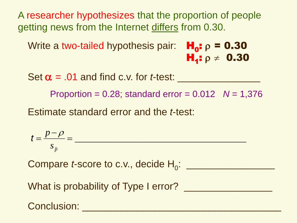
A researcher hypothesizes that the proportion of people

getting news from the Internet differs from 0.30.

Proportion = 0.28; standard error = 0.012 N = 1,376

Write a two-tailed hypothesis pair: H0: = 0.30

H1: 0.30

Set = .01 and find c.v. for t-test: _______________




Conclusion: ____________________________________

_____________________________________

ps

p t

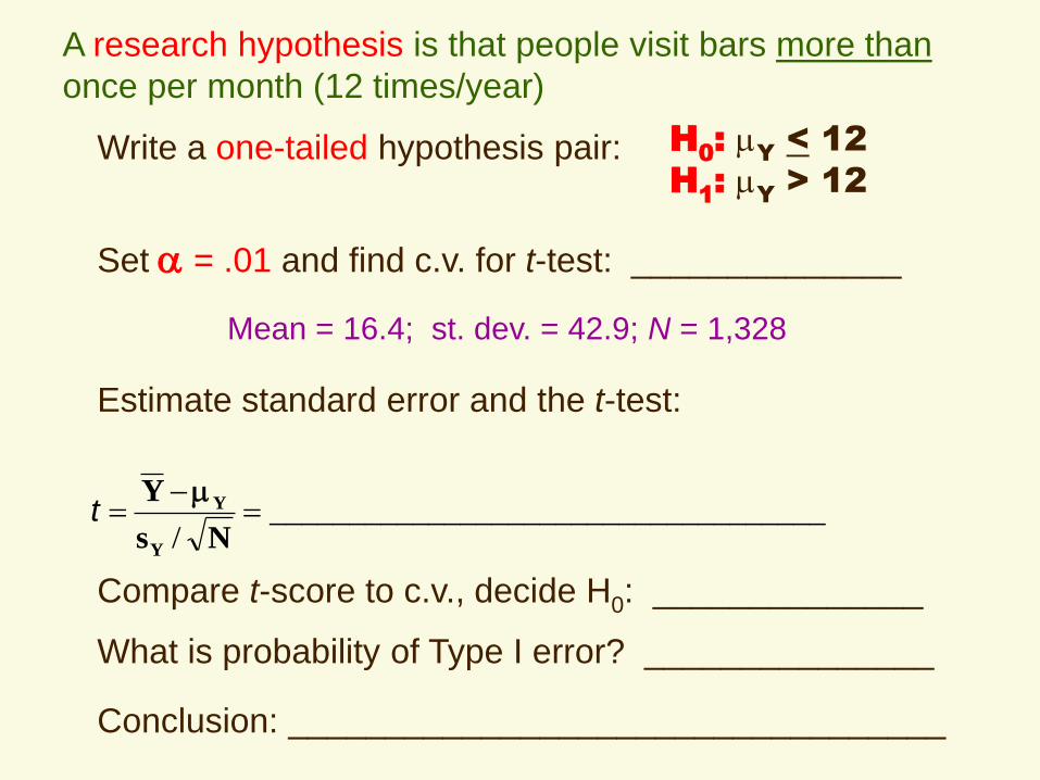
A research hypothesis is that people visit bars more than

once per month (12 times/year)

Mean = 16.4; st. dev. = 42.9; N = 1,328

Write a one-tailed hypothesis pair:

Set = .01 and find c.v. for t-test: ______________


___________________________________/

Ns

Y

Y

Yt

Compare t-score to c.v., decide H0: ______________

What is probability of Type I error? _______________

H0:

Y< 12

H1:

Y> 12

Conclusion: __________________________________

A demographer hypothesizes that the mean number of

people living in U.S. households is now below 2.50?

Mean = 2.47 people; st.dev. = 1.42; N = 2,023

Write a one-tailed hypothesis pair: H0:

Y≥ 2.50

H1:

Y< 2.50



_____________________________________/

Ns

Y

Y

Yt



Conclusion: ____________________________________

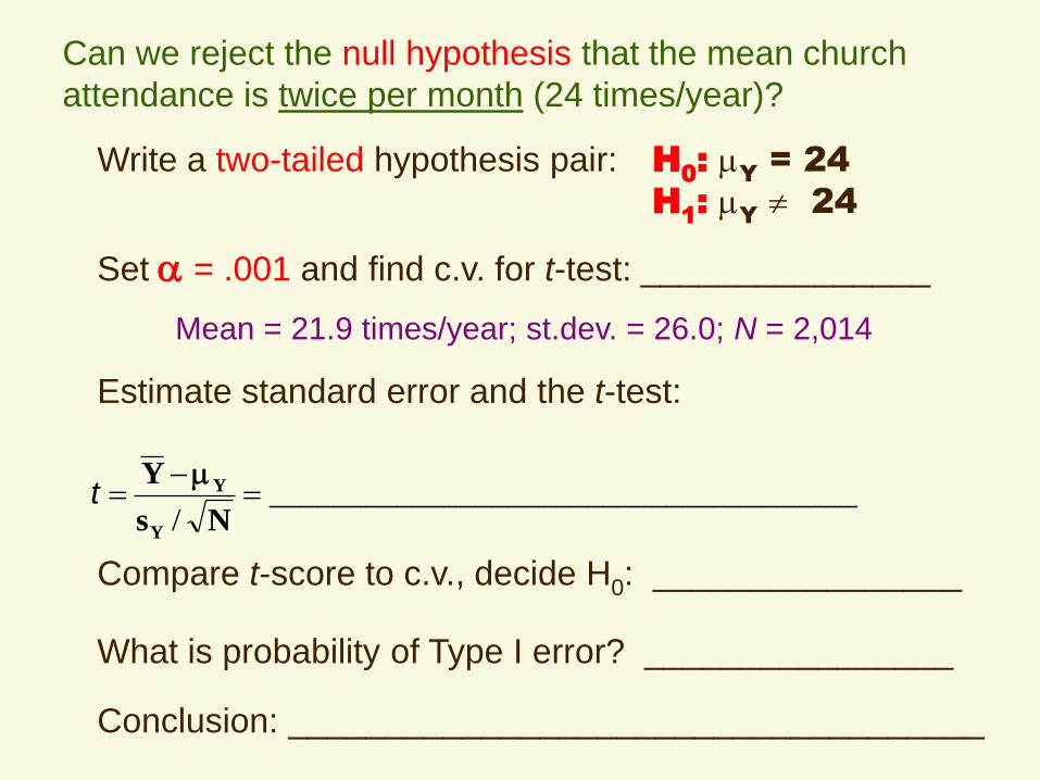
Can we reject the null hypothesis that the mean church

attendance is twice per month (24 times/year)?

Mean = 21.9 times/year; st.dev. = 26.0; N = 2,014

Write a two-tailed hypothesis pair: H0:

Y= 24

H1:

Y 24



_____________________________________/

Ns

Y

Y

Yt



Conclusion: ____________________________________

Documents

Chapter 3 Making Statistical Inferences