Embed Size (px)
Citation preview

On Parameter Estimation in Wireless
Communications, Sensor Array Processing
and Spectral Analysis
Martin Kristensson
TRITA{S3{SB{9856
ISSN 1103{8039
Signal Processing
Department of Signals, Sensors and Systems
Royal Institute of Technology (KTH)
Stockholm, Sweden
Submitted to the School of Electrical Engineering, Royal Institute ofTechnology, in partial ful�llment of the requirements for the degree of
Doctor of Philosophy.

Copyright c 1998 by Martin Kristensson

Abstract
In this thesis, model based parameter estimation in telecommunications,
sensor array processing and spectral analysis is considered. The investi-
gated areas have a wide range of applications, e.g., wireless communica-
tions and sensor array signal processing.
A common theme is the multi dimensional structure of certain appro-
priate vector valued models for the investigated topics. Tools originally
developed in linear algebra are used extensively to estimate the model
parameters.
The �rst investigated topic, direction estimation using sensor arrays,
has been subject to extensive research. Starting with a well known es-
timator, Iterative Quadratic Maximum Likelihood (IQML), a modi�ed
and improved algorithm, Modi�ed IQML (MIQML), is developed. A
statistical analysis of MIQML shows that it is possible to improve its
performance. The improvement is accomplished by proper weighting of
the MIQML criterion function. The so obtained statistically e�cient al-
gorithm (WSF-E) shares many of the appealing properties of the popular
subspace based estimators and is also numerically attractive.
The attention in the thesis is then turned to the estimation of sinu-
soidal frequencies in a time series. This is de�nitely a well investigated
area. Herein, a method which yields optimal parameter estimates within
the class of subspace based algorithms is studied. The method was orig-
inally proposed by Eriksson et. al., but in their analysis of the estimator
several questions were left open. Here, some of the gaps in their analysis
are �lled in and the subspace based method is also related to the Ap-
proximate Maximum Likelihood method (AML) proposed by Stoica et.
al..
The last part of the thesis is devoted to so called blind channel es-
timation in telecommunications. The algorithms considered herein as-
sume that multiple communication channels from the transmitter to the

iv
receiver are available. This is the case in, for example, wireless com-
munication systems where the base stations are equipped with antenna
arrays. A subspace based method is thoroughly investigated and a sta-
tistically optimal version of it is proposed. When identifying a commu-
nication channel using a blind approach, it is crucial to exploit as much
as possible of the structure in the input signal. It is shown that with
certain digital communication schemes, some attractive properties of the
communication signal can be incorporated in a subspace based estima-
tor. This facilitates the use of e�cient second order based algorithms
even when multiple channels between the transmitter and receiver are
not present. Finally, a covariance matching estimator for channel identi-
�cation is proposed. Since the covariance matching estimator possesses
certain optimality properties, it can be used as a benchmark for blind
channel algorithms based only on the second order statistics.

Acknowledgments
It is now approximately four years since my supervisor, Professor Bj�orn
Ottersten, convinced me to enter the PhD program at Signal Processing
at the Royal Institute of Technology (KTH). Bj�orns ideas, encourage-
ment, clear thinking and criticism have in a very positive manner in u-
enced the thesis. Thank you Bj�orn for your guidance and support during
the work.
I would also like to thank my collaborators and co-authors, Professor
Dirk Slock, Doctor Magnus Jansson and Doctor Alexei Gorokhov. The
interaction has been stimulating and has in uenced the thesis to a great
extent.
The sta� at the department has been excellent company during the
lunch breaks (= sandwiches) and the co�ee times. The Wednesdays have
also been particularly enjoyable with \innebandy" as a nice event in the
afternoon.
Finally, I would like to express my gratitude to my parents and my
sister for their great support.


Contents
1 Introduction 1
1.1 Direction Estimation . . . . . . . . . . . . . . . . . . . . . 1
1.2 Frequency Estimation . . . . . . . . . . . . . . . . . . . . 4
1.3 Blind Channel Identi�cation . . . . . . . . . . . . . . . . . 5
1.3.1 Wireless Systems . . . . . . . . . . . . . . . . . . . 5
1.3.2 Antenna Arrays { Multiple Channels . . . . . . . . 7
1.3.3 Channel Identi�cation { Training Sequences . . . . 7
1.3.4 Channel Identi�cation { Blind Methods . . . . . . 9
1.3.5 Blind Algorithms { Traditional Methods . . . . . . 10
1.3.6 Blind Algorithms { Second Order Methods . . . . 13
1.4 The Data Model and the Algorithms Considered in the
Thesis . . . . . . . . . . . . . . . . . . . . . . . . . . . . . 15
1.4.1 A Low Rank Data Model . . . . . . . . . . . . . . 15
1.4.2 Models of the Input Signals and the Noise . . . . . 16
1.4.3 Estimation Methods . . . . . . . . . . . . . . . . . 17
1.4.4 Discussion . . . . . . . . . . . . . . . . . . . . . . . 21
1.5 Thesis Outline and Contributions . . . . . . . . . . . . . . 23
1.6 Future Research . . . . . . . . . . . . . . . . . . . . . . . 26
2 Direction Estimation 29
2.1 Introduction . . . . . . . . . . . . . . . . . . . . . . . . . . 29
2.2 A Data Model . . . . . . . . . . . . . . . . . . . . . . . . . 31
2.3 A Noise Subspace Parameterization . . . . . . . . . . . . . 33
2.3.1 Reparameterization . . . . . . . . . . . . . . . . . 33
2.3.2 Symmetric Solution . . . . . . . . . . . . . . . . . 34
2.4 DML and IQML . . . . . . . . . . . . . . . . . . . . . . . 36
2.4.1 Deterministic Maximum Likelihood (DML) . . . . 37
2.4.2 Iterative Quadratic Maximum Likelihood . . . . . 37

viii Contents
2.5 A Modi�ed IQML Approach . . . . . . . . . . . . . . . . . 38
2.5.1 The Cost Function . . . . . . . . . . . . . . . . . . 38
2.5.2 Implementational Aspects . . . . . . . . . . . . . . 39
2.5.3 Consistency of the Estimate . . . . . . . . . . . . . 40
2.6 Large Sample Properties . . . . . . . . . . . . . . . . . . . 41
2.6.1 Noise Power Estimate . . . . . . . . . . . . . . . . 41
2.6.2 Direction Estimates . . . . . . . . . . . . . . . . . 42
2.6.3 A Simulation Example . . . . . . . . . . . . . . . . 43
2.7 A Statistically E�cient Solution . . . . . . . . . . . . . . 46
2.7.1 The Proposed Algorithm and Analysis . . . . . . . 46
2.7.2 Implementational Aspects of WSF-E . . . . . . . . 48
2.7.3 Simulation Examples . . . . . . . . . . . . . . . . . 49
2.8 Conclusions . . . . . . . . . . . . . . . . . . . . . . . . . . 50
3 Subspace Based Sinusoidal Frequency Estimation 53
3.1 Introduction . . . . . . . . . . . . . . . . . . . . . . . . . . 53
3.2 Data Model and De�nitions . . . . . . . . . . . . . . . . . 55
3.3 Subspace Based Estimator . . . . . . . . . . . . . . . . . . 58
3.4 Preliminaries . . . . . . . . . . . . . . . . . . . . . . . . . 59
3.4.1 Di�erent Sample Estimates . . . . . . . . . . . . . 59
3.4.2 Implications of Toeplitz Structure . . . . . . . . . 60
3.5 Statistical Properties of the Residual . . . . . . . . . . . . 62
3.5.1 The Covariance Matrix of the Residual Vector . . 63
3.5.2 The Rank of the Residual Covariance Matrix . . . 66
3.6 Statistical Analysis . . . . . . . . . . . . . . . . . . . . . . 69
3.6.1 The Optimally Weighted Subspace Estimate . . . 69
3.6.2 Relation to AML . . . . . . . . . . . . . . . . . . . 72
3.7 Implementational Aspects . . . . . . . . . . . . . . . . . . 73
3.8 Conclusions . . . . . . . . . . . . . . . . . . . . . . . . . . 74
4 Communication Systems with Multiple Channels 77
4.1 Introduction . . . . . . . . . . . . . . . . . . . . . . . . . . 77
4.2 Multiple Parallel Channels . . . . . . . . . . . . . . . . . . 78
4.2.1 Di�erent Cases . . . . . . . . . . . . . . . . . . . . 79
4.2.2 Common Framework { Matrix Formulation . . . . 85
4.2.3 On Representations Using the Z-transform . . . . 88
4.3 Correlation Matrices { Notation . . . . . . . . . . . . . . . 89
4.3.1 The Correlation Matrices for the Vector Snapshots 90
4.3.2 The Correlation Matrices in the Windowed System 90
4.4 Assumptions Regarding the System . . . . . . . . . . . . . 91

Contents ix
4.4.1 Statistical Assumptions . . . . . . . . . . . . . . . 91
4.4.2 Simulation Setup . . . . . . . . . . . . . . . . . . . 93
4.4.3 Connections to Practical Systems . . . . . . . . . . 94
4.5 Subspace Ideas and Notations . . . . . . . . . . . . . . . . 97
4.5.1 Basic Notation . . . . . . . . . . . . . . . . . . . . 98
5 Parameterizations and Identi�ability 101
5.1 Subspace Parameterizations . . . . . . . . . . . . . . . . . 102
5.1.1 Signal Subspace Parameterization . . . . . . . . . 102
5.1.2 A Noise Subspace Parameterization . . . . . . . . 103
5.2 Identi�ability . . . . . . . . . . . . . . . . . . . . . . . . . 106
5.2.1 General Results . . . . . . . . . . . . . . . . . . . . 107
5.2.2 Subspace Results . . . . . . . . . . . . . . . . . . . 107
5.3 Identi�ability Implications . . . . . . . . . . . . . . . . . . 108
5.3.1 Temporal Oversampling . . . . . . . . . . . . . . . 109
5.3.2 Spatial Oversampling . . . . . . . . . . . . . . . . 109
5.4 Selection Matrices . . . . . . . . . . . . . . . . . . . . . . 111
5.4.1 Linear Relations . . . . . . . . . . . . . . . . . . . 111
5.4.2 Transformations Between the Parameterizations . 112
6 Weighted Subspace Identi�cation 113
6.1 Early Methods . . . . . . . . . . . . . . . . . . . . . . . . 114
6.1.1 A First Suggestion . . . . . . . . . . . . . . . . . . 114
6.2 Estimation Procedure . . . . . . . . . . . . . . . . . . . . 116
6.2.1 Signal Subspace Parameterization . . . . . . . . . 117
6.2.2 Noise Subspace Parameterization . . . . . . . . . . 118
6.3 Statistical Analysis . . . . . . . . . . . . . . . . . . . . . . 119
6.3.1 The Residual Covariance Matrices . . . . . . . . . 119
6.3.2 The Parameter Covariance Matrix . . . . . . . . . 121
6.4 Special Case { Direction Estimation . . . . . . . . . . . . 124
6.5 Simulation Examples . . . . . . . . . . . . . . . . . . . . . 125
6.6 Conclusions . . . . . . . . . . . . . . . . . . . . . . . . . . 130
7 Further Results on Subspace Based Identi�cation 133
7.1 Introduction . . . . . . . . . . . . . . . . . . . . . . . . . . 133
7.2 Subspace Based Estimator . . . . . . . . . . . . . . . . . . 135
7.3 Structure Emanating from Windowing . . . . . . . . . . . 136
7.4 The Covariance Matrix of the Residual . . . . . . . . . . . 139
7.4.1 Exploiting the Windowed Data Model . . . . . . . 140
7.4.2 Exploiting Properties of the Blocks . . . . . . . . . 142

x Contents
7.4.3 The Covariance Matrix . . . . . . . . . . . . . . . 144
7.5 Performance Analysis . . . . . . . . . . . . . . . . . . . . 147
7.6 Rank of . . . . . . . . . . . . . . . . . . . . . . . . . . . 151
7.6.1 Dimension of . . . . . . . . . . . . . . . . . . . . 152
7.6.2 Special case: L = 2 . . . . . . . . . . . . . . . . . . 153
7.7 Two Channels and High SNR . . . . . . . . . . . . . . . . 160
7.8 Conclusions . . . . . . . . . . . . . . . . . . . . . . . . . . 162
8 Exploiting the Signal Structure 163
8.1 Exploiting the Signal Properties . . . . . . . . . . . . . . 165
8.1.1 One Dimensional Constellations . . . . . . . . . . 165
8.1.2 MSK Modulation . . . . . . . . . . . . . . . . . . . 166
8.2 Alternative Subspace Fitting . . . . . . . . . . . . . . . . 168
8.2.1 An Alternative Covariance Matrix . . . . . . . . . 169
8.2.2 A Low Complexity Solution . . . . . . . . . . . . . 170
8.3 Simulation Results . . . . . . . . . . . . . . . . . . . . . . 171
8.3.1 The Single Channel Case, BPSK and MSK . . . . 173
8.3.2 The Multi Channel Case, BPSK . . . . . . . . . . 176
8.3.3 Correlated Noise . . . . . . . . . . . . . . . . . . . 178
8.4 Conclusions . . . . . . . . . . . . . . . . . . . . . . . . . . 178
9 Blind Identi�cation via Covariance Matching 181
9.1 An Introductory Example . . . . . . . . . . . . . . . . . . 183
9.1.1 The Model and the Estimator . . . . . . . . . . . . 183
9.1.2 The Asymptotical Performance . . . . . . . . . . . 184
9.1.3 A Lower Bound on the Performance . . . . . . . . 185
9.1.4 Numerical Evaluation . . . . . . . . . . . . . . . . 186
9.2 Covariance Matching . . . . . . . . . . . . . . . . . . . . . 187
9.2.1 Hermitian Structure . . . . . . . . . . . . . . . . . 189
9.2.2 Block Toeplitz Structure . . . . . . . . . . . . . . . 190
9.2.3 Least Squares Estimation . . . . . . . . . . . . . . 192
9.3 Statistical Analysis . . . . . . . . . . . . . . . . . . . . . . 192
9.3.1 The Residual Covariance Matrix . . . . . . . . . . 192
9.3.2 The Large Sample Behavior . . . . . . . . . . . . . 193
9.4 Numerical Comparison . . . . . . . . . . . . . . . . . . . . 195
9.4.1 Temporal Window Length N = 3 . . . . . . . . . . 196
9.4.2 Temporal Window Length N = 4 . . . . . . . . . . 198
9.5 Simulation Examples . . . . . . . . . . . . . . . . . . . . . 200
9.6 Conclusions . . . . . . . . . . . . . . . . . . . . . . . . . . 202

Contents xi
A Proofs and Derivations: Direction Estimation 205
A.1 Derivative Expression . . . . . . . . . . . . . . . . . . . . 205
A.2 Analysis of the MIQML Noise Power Estimate . . . . . . 206
A.3 Analysis of the MIQML Direction Estimates . . . . . . . . 208
A.4 A Formula for ��1s . . . . . . . . . . . . . . . . . . . . . . 209
B Proofs and Derivations: Frequency Estimation 211
B.1 A Proof of Lemma 3.1 . . . . . . . . . . . . . . . . . . . . 211
B.2 A Proof of Theorem 3.2 . . . . . . . . . . . . . . . . . . . 214
B.3 A Proof of Lemma 3.2 . . . . . . . . . . . . . . . . . . . . 216
B.4 A Proof of Theorem 3.4 . . . . . . . . . . . . . . . . . . . 218
C Proofs and Derivations: Blind Identi�cation 221
C.1 Mappings Between the Parameterizations . . . . . . . . . 221
C.2 De�nition of Estimation Matrices . . . . . . . . . . . . . . 222
C.3 The Circular Part of the Residual Covariance Matrix . . . 223
C.3.1 Some Additional Notation . . . . . . . . . . . . . . 223
C.3.2 Connection to the Sample Covariance Matrix . . . 224
C.3.3 Covariance Properties of Projected Rxx(0) . . . . 226
C.3.4 Final Results . . . . . . . . . . . . . . . . . . . . . 230
C.4 The Non-Circular Part of the Residual Covariance Matrix 231
C.4.1 The Covariance Matrix of the Non-Circular Part . 231
C.5 The Large Sample Properties of the Sample Covariance
Matrix . . . . . . . . . . . . . . . . . . . . . . . . . . . . . 234
D Notation 239
Bibliography 243


Chapter 1
Introduction
The subjects of this thesis are frequency estimation, direction of arrival
estimation and channel identi�cation. These areas may at a �rst glance
seem rather diverse, but, as will be seen already in this introduction, they
have several properties in common.
This chapter starts with general descriptions of the three considered
application areas. These initial descriptions serve as motivations for the
investigations and derivations of the algorithms treated in the thesis.
The reader already well acquainted with the three areas can proceed
directly to Section 1.4 where the general mathematical framework and al-
gorithms of the thesis are brie y presented. In Section 1.4 the chapters of
the thesis are related using a mathematical framework. This initial chap-
ter is �nally concluded with some future research topics and an outline
of the thesis and its contributions.
1.1 Direction Estimation
Waveforms are in numerous applications measured with sensors located
at di�erent locations in space. The estimation of parameters associated
with these waveforms has for long been an active research area [VB88,
KV96]. The characteristic property of sensor array processing is the multi
dimensional structure of the measurements collected at all the sensors.
The general parameter estimation problem applied to antenna arrays
has numerous applications. An obvious application is radar processing
where the directions and the elevations to far �eld sources are estimated.

2 1 Introduction
The rapid development in wireless communication systems has resulted in
a rather new research area. To increase the capacity (number of concur-
rent users) of the wireless communication systems, many base stations are
nowadays equipped with antenna arrays. The knowledge of the properties
of these arrays from radar applications has accelerated the development
of antenna arrays aimed for the wireless communication systems. Exam-
ples of other application areas are manufacturing and analysis/treatment
methods in medicine.
A natural way to approach the parameter estimation problem in array
signal processing is to adopt a vector notation and express the relations
of the input and output signals to the system using matrix algebra. Pow-
erful tools in linear algebra can in this way be applied to the parameter
estimation problem.
The notion of subspaces are central in linear algebra. A subspace is
a subset of a space with multiple dimensions. Not all sets of a space are
subspaces, i.e., a subspace must possess certain characteristic properties.
An example of a subspace is a plane through the origin in a three dimen-
sional space; see Figure 1.1. The subspace notion is attractive in signal
z
x
y
Figure 1.1: The shaded plane in this �gure is a two dimensional subspace in
a three dimensional space. A line through the origin in the three dimensional
space is a one dimensional subspace.

1.1 Direction Estimation 3
processing because it describes the received data in an e�cient way. In
addition, subspace representations of data sets can be computed numeri-
cally from the collected data set. By computing the dominating subspace
of the received samples, it is possible to concentrate the investigations of
the data set to a lower dimensional space. This is intuitively appealing
since the noise in the weak subspaces is projected away and an increase
in the signal to noise ratio is achieved in some sense.
The subspace notion has resulted in several so called subspace based
techniques for direction estimation. Some examples are MUltiple Signal
Classi�cation (MUSIC) [Sch81], Estimation of Signal Parameters by Ro-
tational Invariance Techniques (ESPRIT) [Roy86], Method of Direction
Estimation (MODE) [SS90] andWeighted Subspace Fitting WSF [VO91].
The subspace based techniques have several attractive statistical as well
as numerical properties.
The development of multi dimensional methods for parameter estima-
tion in sensor array processing has also provided inputs to several other
research areas where sensor arrays are not present. For example, the
estimation of sinusoidal frequencies in a scalar valued time series does
at �rst not seem to have clear connections with sensor array processing.
However, by arranging the scalar valued data in a particular manner, a
matrix formulation of the frequency estimation problem can be obtained.
It turns out that the methods developed for direction estimation in sen-
sor array processing can be applied directly to this matrix formulation of
the frequency estimation problem. One early subspace based algorithm
for frequency estimation is given in [Pis73]. Other areas inspired by the
sensor array processing methods are blind identi�cation [LXTK96, TP98]
and system identi�cation [VD96].
The development of methods for parameter estimation using sensor
arrays has thus several direct as well as indirect application areas. In
the thesis, Chapter 2 is devoted to direction estimation using an array
with identical sensors uniformly distributed along a line. Such arrays
are frequently referred to as uniform linear arrays, ULA. The goal with
Chapter 2 is to develop subspace based direction estimation algorithms
that are easy to implement in practice. As is clear from this short in-
troduction, the developed algorithms may also serve as inspiration and
guidance in many closely connected research areas. In the introduction
to Chapter 2, related articles are given both in the area of blind identi�-
cation and frequency estimation.

4 1 Introduction
1.2 Frequency Estimation
Many engineers prefer to think in terms of signal properties in the fre-
quency domain rather than signal properties in the time domain. The
reason for this is probably the widespread use of linear and time invariant
�lters in the engineering society. The properties of these �lters are most
easily expressed by using a frequency domain approach.
In many cases, the power distribution of a signal over frequency re-
veals important information of the signal properties. This fact is used in
such diverse �elds as, e.g., inspection of mechanical structures, meteorol-
ogy, seismology and speech analysis/synthesis. In other cases, a data set
is investigated with the goal to �nd hidden periodicities. Hidden period-
icities are frequently observed in many engineering problems but are also
found in economics and medicine.
0 10 20 30 40 50 60 70 80 90 100−4
−3
−2
−1
0
1
2
3
Number of samples
Amplitude
0 0.05 0.1 0.15 0.2 0.25 0.3 0.35 0.4 0.45 0.50
5
10
15
20
25
30
35
Normalized time discrete frequency
Spectrum
content
Figure 1.2: A time discrete signal (left) and its corresponding frequency rep-
resentation (right). The time discrete signal consists of one sinusoid in additive
white Gaussian noise.
The estimation of the Doppler frequency to determine the velocity of
a vehicle is an example where it is necessary to estimate a frequency with
good accuracy. In this case, it is known that the signal should exhibit
a periodical structure and the aim is solely to accurately estimate the
frequency of the periodicity. In Figure 1.2, a signal consisting a pure
sinusoid in additive white Gaussian noise is depicted both in the time
and in the frequency domains. Note that, due to the additive noise, it is
not evident from the time domain representation that there is one dom-
inating frequency. However, the frequency representation clearly shows
the sinusoidal structure of the signal.

1.3 Blind Channel Identi�cation 5
Since the number of applications for frequency estimation is extremely
large, there is a large number of related papers in the literature. For line
spectral analysis of discrete time complex valued processes, two early ref-
erences are [RB74, RB76]. For a more complete list of references see,
e.g., [Sto93] and [Por94]. Subspace based methods have since [Pis73]
been applied successfully to sinusoidal frequency estimation. The already
mentioned MUSIC [Sch81] and ESPRIT [Roy86] are other examples of
subspace based techniques for frequency estimation. In Chapter 3, a
subspace based method for frequency estimation is investigated. The
analysis presented in Chapter 3 is an extensive investigation of a general
method �rst presented in [ESS94]. The investigated method is the best
(in a statistical sense) estimator within the class of subspace based fre-
quency estimators. Several characteristics of the estimator are pointed
out and relations to an estimator with certain optimality properties are
also established.
1.3 Blind Channel Identi�cation
The channel identi�cation methods studied in this thesis are frequently
referred to as blind channel identi�cation algorithms. They identify the
channel from the transmitter to the receiver by observing only the chan-
nel outputs. The investigated class of channel identi�cation methods
uses multi channel models of the communication systems. We start by
showing that these models appear frequently in wireless systems. Next,
training based channel identi�cation and traditional blind techniques are
reviewed. Some motivations for why blind methods are interesting are
given. Finally, the new class of methods studied in this thesis is brie y
overviewed.
1.3.1 Wireless Systems
The introduction of digital wireless communication systems has initi-
ated an extensive research in the �elds of signal processing and digital
communication techniques. In traditional telephony, copper wires and
optical �bers constitute the communication channel from the transmitter
to the receiver. To increase the capacity in these traditional systems,
the telecommunication operators \simply" install additional wires. The
quality of the transmission can in wired systems for example be enhanced
by increasing the output power of the transmitter and thereby making

6 1 Introduction
the communication link less sensitive to noise.
In wireless communications, the same procedure can not be used to
increase the system capacity. This since the physical channel is shared by
all the concurrent users in the system. The available frequency spectrum
is distributed between the operators and the operators then try to use
their share of the spectrum as e�ciently as possible. Contrary to the
wired systems, the quality of the wireless systems can not be enhanced
by increasing the transmitter power. This since the battery in the mobile
station limits the output power.
Initially, the number of users in the wireless systems was low. The
major problem was at this stage how to place and construct the base
stations so as to achieve maximum coverage with a minimum number of
base stations. Cellular systems such as GSM solve the coverage problem
by dividing the area to cover into cells; see Figure 1.3. With a base
These cells share the same
frequencies
Figure 1.3: The cellular structure of the wireless system GSM. The operator
distributes the available frequencies within the cells. The two indicated cells,
separated by the frequency reuse distance, are assigned the same frequencies.
station at the center of each cell, a reasonable signal strength is received
at the mobile station within all the cells in the system. Even if the signal
is damped when it propagates, the mobile will in this way always be close
enough to one base station and can in that way establish a communication
link.
The rapid growth of the number of users has changed the basic prob-

1.3 Blind Channel Identi�cation 7
lem in wireless communications. It is now important to design the sys-
tems in order to maximize the number of concurrent users in the systems.
Since all the users share the same physical medium, they disturb each
other. However, since the signals are damped when they propagate, two
users can share the same frequency if they are located at di�erent posi-
tions. The wireless operators use this fact and distribute their frequencies
within the cell structure. As long as the frequency reuse distance, i.e., the
distance between cells that use the same frequencies, is su�ciently large,
the system performs well. Though, in order to maximize the number of
concurrent users, the frequency reuse distance is to be kept as small as
possible. The system capacity is therefore limited by the maximum tol-
erable amount of interference, i.e., the systems are today in many areas
mostly interference limited.
1.3.2 Antenna Arrays { Multiple Channels
Antenna arrays at the base station have been suggested as a means
to increase the system performance [SBEM90, AMVW91, BS92, ZO95,
God97a, God97b]. Antenna arrays can amplify signals at certain direc-
tions and suppress signals in other directions; see Figure 1.4. Therefore,
systems with antenna arrays can tolerate more interference and the cell
planning can in this way be made more aggressive. The antenna arrays
also make the system more tolerable to the noise level when the system
is noise limited.
The characteristic property of antenna arrays is that the signal is
received by multiple sensors. That is, antenna arrays facilitate multi
dimensional signal processing. Consider a mobile station that transmits
to the base station. The signal leaves the transmitter at the mobile
station and propagates through the air to each of the elements in the
antenna array. Such systems are often called single input, multiple output
systems. The part of the thesis that treats blind identi�cation uses special
properties of these multi dimensional systems.
The channels from the mobile to each element in the antenna array are
in many cases di�erent from antenna to antenna in the receiving array.
It is frequently said that antenna arrays exploit the spatial dimension.
1.3.3 Channel Identi�cation { Training Sequences
A signal is in general distorted on its way from the transmitter to the
receiver. For example, the signal is damped when it propagates, sev-

8 1 Introduction
67 8 9
GSM
1 24 5
3
67 8 9
GSM
1 24 5
3
Desired user
Interfering user
Figure 1.4: With an antenna array it is possible to amplify signals arriving
from certain directions. Signals arriving from other directions can be rejected.
In the �gure, the desired user is of course ampli�ed and the interfering user
is rejected. The shaded areas indicate directions where the directivity of the
array is exploited.
eral delayed replicas of the transmitted signal are visible at the receiver
(echoes), and the phase may be shifted. To facilitate compensation for
these phenomena, a training sequence is in most cases transmitted via the
channel to the receiver. The compensation for the distortion is referred
to as equalization. The training sequence is of course known both to the
transmitter and the receiver. With the help of the known input signal
and the measured output signal from the channel, the receiver determines
the channel. The identi�ed channel parameters determine the structure
of the channel response as a function of time. It is therefore frequently
referred to as the temporal structure of the channel. After the receiver
has identi�ed the channel, the information transfer can begin.
To illustrate the procedure, the digital communication system GSM
is used as an example. In GSM, the information is transmitted in pack-
ages called bursts. Each burst contains a training sequence in the center
and the data streams are appended on each side of this sequence; see
Figure 1.5. At reception, the receiver �rst locates the training sequence
and identi�es the communication channel. The knowledge of the commu-
nication channel is then used to tune the receiver when the data symbols
in the information packages are detected. When the receiver uses an
antenna array for reception, the channel in each branch is identi�ed sep-
arately. For detection, the signals from the branches are combined to

1.3 Blind Channel Identi�cation 9
A data burst.
Information sequences.
Training sequences.
Figure 1.5: Two bursts in the GSM system for mobile communication. The
training sequence is located in the center of each data burst. The time variation
of the channel makes it necessary to retransmit the training sequence in each
new data burst. However, the channel can in most cases be considered constant
within one data burst of 148 symbols.
yield improved detection capabilities when compared to a single antenna
receiver.
1.3.4 Channel Identi�cation { Blind Methods
Communication signals are in general very structured. Since we have
designed the transmitter we know this structure and can thus use this
knowledge in the receiver. In fact, it has been shown [Sat75, God80,
TA83] that the channel can be identi�ed by only studying the outputs of
the channel and not knowing the corresponding inputs. That is, even if
the receiver does not know the actual symbols transmitted in the informa-
tion stream, it can use the structure of the received signal to identify the
channel. Since the receiver does not use information of the corresponding
input symbols, the approach is referred to as blind identi�cation.Why is blind identi�cation interesting? It is clearly seen in Figure 1.5
that the training sequence consumes a part of the capacity of the chan-
nel. If the channel can be identi�ed without this training sequence, this
capacity of the channel can be used for information transfer and speed
up the communication or to increase the e�ciency.
There are other motivations for blind identi�cation as well. For ex-
ample, Godard mentions in [God80] that large computer networks can
in several cases bene�t from blind identi�cation. One advantage with
blind identi�cation is that each computer station can resynchronize to
the rest of the system on its own. If a computer looses synchronization
and/or the channel to that station changes drastically, it can resynchro-

10 1 Introduction
nize to the rest of the system without disturbing the other computers.
This is bene�cial speci�cally in large systems where resynchronization
procedures otherwise disturb the communication. The time variation of
the wireless channels (the environment changes) highlights the need for
channel identi�cation in mobile communication systems.
In some communication scenarios a training sequence is not avail-
able. This is the case in many military systems where the enemy is
eavesdropped. However, the training sequence may be unknown also in
many commercial communication scenarios. For example, consider the
case when a base station in a cellular network receives the signal from
a mobile station within the cell and at the same time is disturbed by a
user in a neighboring cell. To suppress the interfering user it is bene�cial
to know the channel from the interfering user to the receiving base sta-
tion. However, the base station does in most cases not know the training
sequence of the interfering user. This since it is too complicated for the
base stations to keep track of the training sequences of all the mobiles
in the system. Hence, the only way to determine the channel to the
interfering user is to use blind methods [KO98a].
Interference rejection is also of interest in Code Division Multiple
Access systems (CDMA). Several papers exploiting ideas found in blind
identi�cation has been published in this area. A review of methods for
CDMA interference suppression can be found in [Mad98].
1.3.5 Blind Algorithms { Traditional Methods
There are mainly two classes of blind channel identi�cation algorithms;
those that exploit the special structure of single input, multiple output
systems and those that do not. In the thesis, the single input, multiple
output systems are considered, but �rst a brief review of the \traditional"
methods is given.
In traditional blind identi�cation methods it is assumed that the time
discrete representation of the system is single input, single output1. The
single input, single output system is depicted in Figure 1.6. In this �gure,
d(t) are the time discrete input data symbols and x(t) is the received time
discrete data sequence. The unknown impulse response of the time dis-
crete channel is denoted by h(t) and the additive noise by n(t). The blind
identi�cation problem for scalar valued channels is now simply stated ac-
1It is possible to modify the \traditional" methods to apply to single input, multiple
output systems as well. For notational convenience, only the scalar valued case is
treated here.

1.3 Blind Channel Identi�cation 11
cording to: Given only measurements of the outputs, x(t), determine h(t)
and the input symbols d(t)!
+h(t)d(t)
n(t)
x(t)
Figure 1.6: A scalar valued digital communication link. This is the most basic
model used for a communication channel. The input signals are transmitted via
a channel, h(t), that introduces linear distortion. White noise, n(t), is added
at the output.
The �rst step in most of the traditional blind identi�cation methods
is to �lter the received signal adaptively. If the output of the adaptive
�lter does not share the properties of the communication signal for the
particular system of interest, the adaptive �lter is changed. After con-
vergence the output from the adaptive �lter shares all the properties of
the communication signal. The overall structure of a traditional blind
receiver is given in Figure 1.7.
The key issue in the traditional methods is how to adapt the receiver
�lter. A common approach is to take the output, d(t), from the adaptive
time discrete �lter and compute an error signal, �(t). The function, �(�),used to compute the error signal exploits the properties of the particular
communication signal. For example, consider the case of binary signaling,
i.e., d(t) 2 f�1g. Since jd(t)j = 1 in this case, a nice error function is
�(d(t)) = jjd(t)j � 1j: (1.1)
Here, jxj denotes the absolute value of x. In the absence of noise it is
clear that, with this choice of �(t), the error signal, �(t), is zero when g(t)
compensates fully for the distortion introduced by h(t). The error signal
can therefore be used to adapt the receiver �lter. With noise present,
g(t) is an approximative compensation.
An early blind equalization technique for multi level digital commu-
nication systems was proposed by Sato [Sat75]. As presented in that
paper the algorithm only applies to amplitude modulated systems, but,

12 1 Introduction
+ g(t) �(�) �(t)d(t)x(t)h(t)
n(t)
d(t)
Figure 1.7: The structure of many traditional blind identi�cation receivers.
The time discrete adaptive receiver �lter, g(t), is supposed to compensate for
the distortion introduced by h(t). The output from g(t), d(t), should thus be
close to d(t). The function �(�) generates an error signal, �(t), that is used to
adapt the receiver �lter.
as shown in [BG84], it is possible to generalize the method also to com-
bined amplitude and phase modulation. Alternative cost functions for
the combined amplitude and phase modulation case are given by Godard
in [God80]. A special case of the methods suggested by Godard is the well
known Constant Modulus Algorithm (CMA) [JSE+98] which exploits the
fact that some communication signals are of constant amplitude.
All methods presented up to now formulate a cost function, �(�), thatexploits some of the special characteristics that the communication signal
exhibits. The cost functions rely on the fact that higher order statistics
of communication channels uniquely specify the system. A problem with
these methods is their slow convergence rate. In general, they require
thousands of samples before the equalizer coe�cients converge. An alter-
native method suggested in [Ses94, GW95] is to use a maximum likelihood
approach in order to jointly estimate the channel coe�cients and the data
symbols. Although this approach guarantees optimal performance and
therefore also fast convergence rate, the huge numerical complexity limits
its usefulness.
The model in Figure 1.6 is not restricted only to digital communi-
cation systems. Therefore, blind identi�cation (or deconvolution) of one
dimensional systems arises in other areas as well, e.g., image restoration
and seismic signal processing. In [Hay94] more examples of alternative
applications are given together with collected works and references to pa-
pers in traditional blind identi�cation. A more recent survey of the blind
identi�cation �eld is found in [TLH98].
The methods studied in this thesis are an alternative to the traditional
ones when fast convergence is important. A short background to these

1.3 Blind Channel Identi�cation 13
\new" methods is given in the next section.
1.3.6 Blind Algorithms { Second Order Methods
It is known that when the moments of the received signal are estimated,
the time to convergence is longer for higher order moments than for sec-
ond order moments. Therefore, fast convergence of methods based only
on statistical properties of the output signals implies that only second
order properties can be used. The second order properties are the statis-
tical expected values of quadratic combinations of the outputs, e.g., x2(t)
and x(t)x(t� 1). However, it is easily established that unique identi�ca-
tion of the scalar valued channel in Figure 1.6 is impossible using only
the information contained in the second order output statistics. This is
the reason for working with higher (than 2) order statistics in the case of
a single communication channel. In the scalar valued case, higher order
statistics add the missing information necessary for unique identi�cation
of the channel coe�cients.
The idea behind the recently introduced second order based methods
[TXK91, LXTK96, TP98] is to use the additional information present in
the outputs of a multi channel system. See Figure 1.8 for an illustra-
tion of a time discrete representation of a multi channel communication
system. As we have seen earlier, this model arises frequently in wireless
communication systems which employ antenna arrays at the base station.
The system model in Figure 1.8 incorporates both the spatial structure
(several channels) and the temporal properties (modeled independently
by hi(t) in each branch). Signal processing algorithms applied to such
systems are sometimes called spatio-temporal methods [PP97].
It has been established that unique identi�cation of the channels h1(t)
to hL(t) is possible by studying only the second order statistics of the
outputs x1(t) to xL(t). This fact was early exploited in the paper by
Tong et. al. [TXK91]. It has also been established that ordinary single
input, single output communication systems can under certain assump-
tions alternatively be viewed as a single input, multiple output system
[TXK91]. This is possible due the periodic structure, sometimes referred
to as cyclostationarity, of digital communication signals,
The new multi channel formulation of the blind identi�cation prob-
lem facilitates the application of methods common in system identi�ca-
tion and sensor array processing. The �rst paper written by Tong et.
al. applied a so called subspace based method for the identi�cation of
the channel coe�cients. Similar subspace algorithms exist for direction

14 1 Introduction
+
+
+xL(t)
h1(t)
h2(t)
hL(t)
d(t)
...
n1(t)
n2(t)
nL(t)
x1(t)
x2(t)
Figure 1.8: A discrete time single input, multiple output communication
system.
of arrival estimation in sensor array processing. After the �rst paper
many ideas from sensor array processing were converted to �t into the
framework of blind channel identi�cation. Other suggested subspace ap-
proaches are presented in [Ton92, SP94, MDCM95, GS96].
The advantage with the second order based methods is the fast conver-
gence rate (on the order of hundreds of symbols). The main disadvantage
is problems with identi�ability for special con�gurations of multi channel
systems. For example, if all channels in the multi channel systems are
equal, then the outputs obviously do not contain more information than
an ordinary scalar valued channel. For the second order methods to work
properly, the available channels must be signi�cantly di�erent to assure
identi�ability.
In Chapters 4 to 5 a more thorough and mathematical description
of second order based blind methods is given. In Chapter 6 a subspace
based estimator �rst proposed in [MDCM95] is analyzed and a statis-
tically optimal version is derived. In some communication systems the
modulation format can be used e�ectively in the blind channel identi�-
cation algorithms. Examples on how to do this is given in Chapter 8.
Finally, a so called covariance matching estimator is given in Chapter 9.
The covariance matching estimator exhibits certain statistical properties

1.4 The Data Model and the Algorithms Considered in the Thesis 15
which makes a comparison with the estimator proposed in Chapter 6
interesting.
1.4 The Data Model and the Algorithms Con-
sidered in the Thesis
The areas covered in this thesis can all be formulated using a matrix
framework. Herein, the properties of the general matrix model exploited
in the thesis are outlined. Di�erences as well as similarities of the di�erent
topics are pointed out.
1.4.1 A Low Rank Data Model
All the investigated problems in the thesis can be modeled as a complex
valued linear time invariant system with d inputs and m outputs. The
inputs are collected in the d�1 vector s(t) and the outputs are contained
in the m � 1 vector x(t). Since the system is linear with �nite memory,
the mapping from the input signals to the output signals can be described
by a matrix equation
x(t) = A(�)s(t) + n(t); t = 1; : : : ; N: (1.2)
Here, A(�) is an m � d matrix which is parameterized by the elements
in the column vector �. The m� 1 vector n(t) represents additive com-
plex valued Gaussian noise. The goal in the thesis is to estimate the
parameter vector � associated with the system by observing the output
signals x(1); : : : ;x(N). The parameter vector will consist of sinusoidal
frequencies, directions of arrival and channel parameters depending on
the application.
A characteristic property of the topics treated in the thesis is that
the number of outputs of the matrix model is strictly greater than the
number of inputs, i.e., m > d. This makes the matrix A(�) \tall", i.e.,
it has more rows than columns. In addition, the columns in A(�) are
linearly independent in all the three investigated areas. That is, the
columns in A(�) span a d-dimensional subspace of the m-dimensional
vector space. The speci�c parameterization of A(�) is of course di�erent
for the di�erent areas in the thesis.
In some cases, it is possible to �nd a full rank m � (m � d) matrix,
B(�), such that its columns span the complete null space of A(�); that

16 1 Introduction
is,
A�(�)B(�) = 0d�(m�d); 8�: (1.3)
Here, 0d�(m�d) is a d � (m � d) matrix with all the elements equal to
zero and (�)� denotes complex conjugate transposition. Since the noise
free received signal is constrained to the space spanned by the columns in
A(�), the matrix B(�) is said to be a parameterization of the noise sub-
space. The noise subspace parameterization is particularly useful when
subspace based estimation is considered and when the matrixB is linearly
parameterized by the elements in �.
1.4.2 Models of the Input Signals and the Noise
The di�erences between the investigated areas are not only restricted to
di�erent structures of A(�), but are also manifested in di�erent assump-
tions on the input process s(t) and the additive noise n(t).
In general, both the input signal, s(t), and the additive noise, n(t),
are considered to be realizations of stochastic processes. The covariance
matrices for these two vector valued random variables are here denoted
by
Rss(�) = Efs(t)s�(t� �)g; (1.4)
Rnn(�) = Efn(t)n�(t� �)g: (1.5)
The input signal and the noise are throughout the thesis considered to
be independent of each other and the covariance matrix of the output
vector is therefore
Rxx(�) = Efx(t)x�(t� �)g = A(�)Rss(�)A�(�) +Rnn(�): (1.6)
Note that the covariance matrices Rss(�) and Rnn(�) may contain ad-
ditional unknown parameters, denoted by , compared to the parame-
ters determining the low rank matrix A(�). However, since the primary
interest is in �, the elements in are mostly considered as nuisance
parameters.
In addition to being independent of the input signal, the noise process
is assumed to satisfy
Rnn(0) = �2I; (1.7)

1.4 The Data Model and the Algorithms Considered in the Thesis 17
where the noise power �2 is considered unknown and I is the m�m iden-
tity matrix. The properties of the covariance matrix Rss(0) are di�erent
for the three subjects treated.
It turns out that the particular structure ofRss(�) andRnn(�) greatly
a�ects the properties of the estimators considered in this thesis. In the
most simple case (array processing) the input process and the noise pro-
cess can be considered as temporally uncorrelated, i.e.,
Rss(�) = Rss(0)�(�); (1.8)
Rnn(�) = Rnn(0)�(�); (1.9)
where �(�) is the Kronecker delta. However, the assumption of temporally
uncorrelated processes is not valid for the sinusoidal frequency estimation
problem or for the channel identi�cation area.
1.4.3 Estimation Methods
In the thesis, both subspace based estimators and covariance matching es-
timators are considered. In this section, these estimators are commented
on together with a description of the maximum likelihood estimator.
The Maximum Likelihood Estimator
Since the maximum likelihood algorithm constitutes a systematic ap-
proach to parameter estimation it has been thoroughly investigated in the
literature. In many cases, the estimator reaches the Cram�er-Rao bound
[Cra46] on the asymptotical parameter estimation error covariance ma-
trix. The Cram�er-Rao bound is a lower bound on the estimation error
covariance matrix of the parameter estimates for all unbiased estimators.
To de�ne the maximum likelihood estimator of the model parameters,
the probability density function of the received vector samples is needed.
For simplicity, de�ne the vector XN that contains all the observed vec-
tors,
XN =�xT (1) xT (2) : : : xT (N)
�T: (1.10)
Here, (�)T denotes transposition. The maximum likelihood estimates are
obtained as follows
f�; g = argmax�;
fX(XN ;�; ); (1.11)

18 1 Introduction
where fX(XN ;�; ) is the probability density function of the received
snapshots evaluated at the observationXN . Note that, sinceXN is deter-
ministic once the received samples are observed, the function fX(XN ;�; )
is purely a function of � and and is thus deterministic. Given the sta-
tistical framework of the observed random process, it is thus straight
forward to formulate the maximum likelihood estimator.
The maximum likelihood estimator has been considered in the litera-
ture for all the investigated topics in the thesis. In the direction of arrival
estimation area, there exist two di�erent maximum likelihood estimators
[BM86, OVSN93] depending on the model assumed for the signal vec-
tors, s(t). If the signal vectors, s(t), are assumed to be a realization of
a stochastic process, then the so called stochastic maximum likelihood
estimator (SML) is obtained. If, on the other hand, the signal vectors
are considered to be unknown but deterministic parameters, the so called
deterministic maximum likelihood estimator (DML) is obtained. Surpris-
ingly, these two estimators behave di�erently. Descriptions of the max-
imum likelihood estimator for the sinusoidal case can be found in, e.g.,
[RB74, RB76, SMFS89, Por94]. For the blind channel estimation topic,
the maximum likelihood estimators can be found in [Hua96, TP98, CS96].
The advantage with the maximum likelihood estimator is that it
reaches the Cram�er-Rao lower bound on the asymptotical estimation er-
ror covariance matrix in many cases. The drawback is that the parameter
estimates can not be solved for analytically except in some very special
cases. Since the criterion function often exhibits local minima, the numer-
ical search procedures associated with the maximum likelihood estimator
are often complicated.
The Covariance Matching Estimator
The covariance matching estimator is also commonly referred to as the
method of moments [Por94]. The covariance matching estimator is basi-
cally a least squares �t of the estimated sample covariance matrices and
the parameterized versions thereof.
To de�ne the covariance matching estimator, collect the covariance
matrices for the time lags � = �k; : : : ; k in one matrix
�R =�Rxx(�k) Rxx(�k + 1) : : : Rxx(k)
�: (1.12)
In many cases, it is easier to consider the columns in �R when they are
placed after each other in one large column vector. With the vectorization

1.4 The Data Model and the Algorithms Considered in the Thesis 19
operator [Gra81, Bre78] this large vector is compactly written
r = vec[ �R]: (1.13)
Since the model of the signals is parameterized by � and , the vector
r is a function of both � and . The sample estimate corresponding to
r is computed from the received snapshots and is denoted by r. The
covariance matching estimator can with these notations be written
f�; g = argmin�;
(r (�; )� r)�W(�; ) (r (�; )� r) : (1.14)
Note that the weighting matrix, W, is possibly parameter dependent.
The covariance matching estimator has been applied to the direction
estimation problem in, e.g., [KB90, WSW96, OSR98]. Applications to
blind channel identi�cation are found in, e.g., [GH97, ZT97, KO97].
The covariance matching estimator has the appealing property that
if W is chosen optimally, the estimator is the best possible of all estima-
tors based on the covariance matrices for lags from �k to k. However,
the criterion function can in most cases not be minimized analytically
and the parameter estimates must therefore in general be obtained by
numerical search procedures. Nevertheless, the estimator constitutes a
useful benchmark to which other estimators may be compared.
The Subspace Based Estimator
Subspace based estimators exploit properties of the eigenvalue decompo-
sition of the covariance matrix Rxx(0). Let d0 be the rank of the covari-
ance matrix, Rss(0), of the signal vector. The eigenvalue decomposition
of Rxx(0) is given by
Rxx(0) =
mXk=1
�keke�
k= Es�sE
�
s+En�nE
�
n= Es�sE
�
s+ �2EnE
�
n;
(1.15)
where
Es =�e1 : : : ed0
�(1.16)
En =�ed0+1 : : : em
�(1.17)
�s = diag[�1; : : : ; �d0 ] (1.18)
�n = diag[�d0+1; : : : ; �m] (1.19)

20 1 Introduction
and where the eigenvalues �k are numbered in descending order. The
notation diag[�] denotes a matrix with the indicated elements on the
diagonal and with zero valued entries on all other positions. Since the
covariance matrix Rxx(0) is Hermitian, the eigenvectors can be chosen
so that they are orthogonal. The eigenvectors corresponding to the d0
largest eigenvalues are collected in the matrix Es and the span of this
matrix is called the signal subspace. The eigenvectors corresponding to
the m� d0 smallest eigenvalues are collected in En and the span of this
matrix is termed the noise subspace. Estimates of the noise and signal
eigenvector matrices computed from the received snapshots are denoted
by En and Es, respectively.
Since Rnn(0) = �2I, it is easy to verify that the column span of Es
is contained in the column span of A(�); that is,
spanfEsg � spanfA(�)g: (1.20)
In addition, since A(�) and B(�) are orthogonal matrices, it holds that
spanfEsg ? spanfB(�)g: (1.21)
In the problems investigated in this thesis, the parameter vector � is
uniquely identi�able by the orthogonality property between the noise
and signal subspaces. That is, if
B�(�0)Es = 0(m�d)�d (1.22)
holds for some �0, then �0 = � = the true parameter vector. When an
exact estimate of the signal subspace is not available, the orthogonality
property does not hold exactly. In that case it makes sense to estimate
the parameters according to
f�; g = argmin�;
vec�[B�(�0)Es]W(�; ) vec[B�(�0)Es]: (1.23)
Note that the nuisance parameters collected in only a�ect the weight-
ing matrix. That is, with identity weighting, the nuisance parameters
disappear in an appealing way in the subspace based estimator.
When the covariance matrix Rss(0) is full rank, the relation in (1.20)
holds exactly, i.e.,
spanfEsg = spanfA(�)g: (1.24)
In this case it thus also true that
spanfEng ? spanfA(�)g: (1.25)

1.4 The Data Model and the Algorithms Considered in the Thesis 21
WhenRss(0) is full rank, it is thus possible to formulate a subspace based
estimator based on En as well. The parameter estimates obtained with
such an algorithm are given by
f�; g = argmin�;
vec�[A�(�)En]W(�; ) vec[A�(�)En]: (1.26)
Since the noise and signal subspaces are orthogonal complements, the
estimators are equivalent if the weighing matricesW are chosen properly.
The subspace based estimator is particularly attractive when at least
one of the matrices A(�) or B(�) is parameterized linearly by the el-
ements in �. In that case, the parameter estimates in (1.23) or (1.26)
can be solved for analytically and the numerical search associated with
many other estimators is avoided. Though, despite e�cient algorithms
exist for the computation of Es and En, the eigenvalue decomposition of
the sample covariance matrix is still intense. However, subspace based
estimators are still preferable to covariance matching and maximum like-
lihood algorithms in many cases.
1.4.4 Discussion
Herein, the contents of the thesis are related to the data model and the
estimation methods discussed in the previous sections. The central issue
of the thesis is parameter estimation for low rank data models. The
thesis considers such models valid for frequency, directions of arrival and
channel parameter estimation.
Direction Estimation
Since low rank data models appear naturally when data is collected with
several sensors, the �rst topic in the thesis is direction of arrival esti-
mation. The estimation of directions of arrival is covered extensively in
the literature. The maximum likelihood estimators [BM86, OVSN93], the
subspace based procedure [Sch81, Roy86, SS90, VO91] and the covariance
matching algorithm [WSW96, KB90, OSR98] have all been investigated
in great detail.
Chapter 2 starts with an investigation of the Iterative Quadratic Max-
imum Likelihood Method [BM86]. The inconsistency of this estimator
[SLS97] is discussed and alternative consistent and statistically e�cient
(methods that reach the Cram�er-Rao lower bound) approaches are pro-
posed. The methods proposed in Chapter 2 all avoid the eigendecompo-

22 1 Introduction
sition of the sample covariance matrix that is necessary in most subspace
based procedures.
The assumption of temporally uncorrelated vector snapshots simpli-
�es the construction and the analysis of the treated algorithms consider-
ably.
Frequency Estimation
The optimal subspace based estimator is derived both within the si-
nusoidal frequency estimation and the channel estimation frameworks.
Since the optimal subspace based estimator for frequency estimation
[ESS94] was established prior to the work in this thesis, the focus for
the subspace based frequency estimator in Chapter 3 is on questions that
were left open in [ESS94]. These questions are, e.g., the rank and range
properties of the residual covariance matrix of the estimator, the opti-
mal weighting matrix in the general case, and relations to the covariance
matching type estimator (AML) proposed by Stoica et. al. in [SHS94].
Contrary to array processing, the received data snapshots are in fre-
quency estimation temporally correlated. This complicates the analysis
of the subspace based estimator a great deal when compared to the array
processing case. It is shown that several properties of the subspace based
estimator are closely related to the temporal properties of the snapshots.
Blind Channel Identi�cation
For the blind channel identi�cation area, the optimal counterpart of the
subspace based estimator presented in [MDCM95] is derived in Chap-
ter 6. In Chapter 7, several properties of this optimal estimator are
investigated further. Since the statistical assumptions of the underlying
stochastic processes are similar to the sinusoidal frequency estimation
topic, Chapter 7 and Chapter 3 have several common divisors.
The section of the thesis that considers blind channel estimation is
then in Chapter 8 concerned with subspace based estimators applied to
some particular communication systems. It is shown that by incorpo-
rating information regarding the particular modulation format in some
communication systems, the estimator can be improved signi�cantly. In
addition, the exploitation of these properties also facilitates subspace
based estimation in cases when this is not possible without taking these
particular properties into account.
The section of the thesis that considers blind channel estimation is

1.5 Thesis Outline and Contributions 23
concluded with Chapter 9 that contains the derivations of a covariance
matching estimator for blind channel estimation. The performance of the
covariance matching estimator is compared numerically to the subspace
based estimator derived in Chapter 6.
1.5 Thesis Outline and Contributions
This section is a chapter by chapter outline of the thesis and also serves as
a presentation of the contributions on which the thesis is based. Observe
that the material in the thesis is not presented in chronological order,
but rather in a \logical" order.
Chapter 2
A major part of the thesis is based on estimation of parameters in low
rank matrix models. Here, the low rank properties of a well known model
for sensor array processing is used to estimate the directions of arrival
of the impinging signals on the array. This is an area that has been in-
tensively investigated in the literature. Several methods exist that reach
or are close the Cram�er-Rao lower bound on the estimation error co-
variance. One such estimator is the weighted subspace �tting algorithm
(WSF) which is also known as MODE.
The core idea in the chapter is to obtain a statistically e�cient esti-
mator that is also computationally attractive. The chapter starts with
a study of deterministic maximum likelihood (DML) and the iterative
quadratic maximum likelihood (IQML) method. It is shown that the
bias in the IQML method can be avoided by using proper constraints
on the parameterization. In addition, based on the investigation of the
unbiased version of IQML, it is shown that the eigendecomposition of
the sample covariance matrix which is needed in WSF can be avoided
without any performance loss.
Parts of the material in the chapter have been presented at the Inter-
national Conference on Acoustics, Speech, and Signal Processing (ICASSP)
and a paper version is submitted to Signal processing:
Martin Kristensson, Magnus Jansson, and Bj�orn Ottersten. Modi-
�ed IQML and a statistically e�cient method for direction estima-
tion without eigendecomposition. In International Conference onAcoustics, Speech, and Signal Processing, Seattle, May 1998. IEEE.

24 1 Introduction
Martin Kristensson, Magnus Jansson, and Bj�orn Ottersten. Modi-
�ed IQML and weighted subspace �tting without eigendecomposi-
tion. Submitted to Signal Processing.
Chapter 3
The estimation of sinusoidal frequencies is also a well studied �eld in
signal processing. In the literature, ESPRIT and MUSIC have been
successfully applied to this estimation problem. In addition, a statisti-
cally attractive Markov like subspace based procedure has been suggested
[ESS94]. In this chapter, the Markov like procedure is re-investigated.
Several results regarding rank, performance and optimality are derived.
For example, it is shown that the Markov like procedure is asymptotically
equivalent to the AML (Approximative Maximum Likelihood) method
proposed by Stoica et. al. [SHS94].
The chapter exploits several properties of the sample covariance ma-
trix in order to establish certain rank results. It turns out that a similar
approach may be applied to the blind estimation problem studied in the
following chapters. Speci�cally, this chapter may serve as an introduction
to Chapter 7.
The material in the chapter is submitted to the International Con-
ference on Acoustics, Speech, and Signal Processing (ICASSP) and an
article version is submitted to IEEE Transactions on Signal Processing:
Martin Kristensson, Magnus Jansson, and Bj�orn Ottersten. On
subspace based sinusoidal frequency estimation. Submitted to In-
ternational Conference on Acoustics, Speech, and Signal Process-
ing.
Martin Kristensson, Magnus Jansson, and Bj�orn Ottersten. Fur-
ther results and insights on subspace based sinusoidal frequency
estimation. Submitted to IEEE Transactions on Signal Processing.
Chapters 4 and 5
These two chapters serve as an introduction to the channel identi�cation
part of this thesis. The multi channel structure of certain communication
channels is commented on and several well known results regarding pa-
rameterizations and identi�ability are surveyed. If the reader is familiar
with the subject, these chapters can be used as a reference when reading
the following chapters.

1.5 Thesis Outline and Contributions 25
Chapter 6
The blind identi�cation of communication channels is studied in this
chapter. The multi channel structure is important when considering
transmission of information via wireless communication channels. The
�rst proposed algorithm is an optimally weighted version of the estimator
proposed by Moulines et. al. [MDCM95]. The second proposed algorithm
exploits a parameterization of the noise subspace �rst presented by Slock
[Slo94]. The chapter includes a thorough statistical analysis of the in-
vestigated class of estimators as well as derivations of optimal weighting
matrices in the proposed Markov like procedure.
The material in the chapter has been presented at the International
Conference on Acoustics, Speech, and Signal Processing and an article
version of the chapter can be found in IEEE Transactions on Signal Pro-
cessing:
Martin Kristensson and Bj�orn Ottersten. Statistical analysis of a
subspace method for blind channel identi�cation. In InternationalConference on Acoustics, Speech, and Signal Processing, volume 5,pages 2437{2440, Atlanta, Georgia, May 1996. IEEE.
Martin Kristensson and Bj�orn Ottersten. A statistical approach to
subspace based blind identi�cation. IEEE Transactions on SignalProcessing, 46(6), June 1998.
Chapter 7
This chapter contains further investigations of the algorithm in Chapter 6.
The structure present in the sample covariance matrix is exploited in or-
der to establish a larger class of optimal weighting matrices in the Markov
like procedure. In addition, the special case of two parallel communica-
tion signals is studied in detail. The chapter is similar to Chapter 3, but
here the studied estimation problem is slightly di�erent.
Parts of the results appear in:
Martin Kristensson and Bj�orn Ottersten. Further results on opti-
mally weighted subspace based blind channel estimation. In Pro-ceedings of the 32th Asilomar Conference on Signals, Systems andComputers, Paci�c Grove, CA, November 1998.

26 1 Introduction
Chapter 8
Herein, methods are presented that exploit the signal constellation prop-
erties of certain communication systems. It is in general di�cult to take
these properties into account in the channel estimation procedure. This
is speci�cally true when a subspace based approach is used. The chapter
contains descriptions on how these properties may be exploited. Simula-
tion results indicate the potential of the suggested methods.
The material has been presented at:
Martin Kristensson, Dirk T.M. Slock, and Bj�orn Ottersten. Blind
subspace identi�cation of a BPSK communication channel. In
Proceedings of the 30th Asilomar Conference on Signals, Systemsand Computers, Paci�c Grove, CA, November 1996.
Chapter 9
In this chapter, a covariance matching estimator for the blind channel
estimation problem is presented. The presented covariance matching es-
timator is optimal in the sense that it takes all the information present
in the second order moments into account. The main contribution in the
chapter is the comparison of the performance for the subspace based es-
timator in Chapter 7 with the lower bound that the covariance matching
estimator represents. Theoretical as well as simulation results are given.
The material has been presented at the conference Signal Processing
Advances in Wireless Communications:
Martin Kristensson and Bj�orn Ottersten. Asymptotic comparison
of two blind channel identi�cation algorithms. In Proceedings ofSPAWC97, Signal Processing Advances in Wireless Communica-tions, Paris, France, April 1997. IEEE.
1.6 Future Research
The �rst two sections of the thesis, direction estimation and spectral
analysis, consider topics that have been subject to extensive research in
the literature. This implies that the number of open research problems in
these areas are limited. Since the blind identi�cation of communication
channels is more recent, more open problems can be found there.
One general approach that has been treated in the thesis is the window
process used to obtain a low rank vector valued model of a system. A low

1.6 Future Research 27
rank model is attractive since then powerful subspace based estimation
schemes can be applied. One particular feature with subspace based es-
timation is that, once the eigenvalue decomposition has been computed,
the parameter estimates can in many cases be obtained without compli-
cated numerical search procedures. In addition, there exist powerful and
stable numerical methods that computes the eigenvalue decomposition.
However, as is shown in the thesis, the procedure results in a (block)
Toeplitz covariance matrix to which the eigenvalue decomposition is ap-
plied. Since the same element is repeated on several positions in this
matrix, the dimension of the matrix valued statistic is larger than neces-
sary. Hence, it seems natural to investigate schemes (covariance match-
ing) that do not repeat the same covariance matrix element more than
once in the cost function. The question is whether or not there exist
e�cient numerical methods that solve for the parameters even for these
schemes. Furthermore, the unweighted subspace based procedure often
outperforms the unweighted covariance matching estimator. If, in addi-
tion, a low complexity weighting of the covariance matching estimator
that yields performance close to subspace based estimators can be found,
an estimator with both attractive statistical as well as numerical proper-
ties is obtained.
The area of blind channel estimation is still under development. Most
of the standard type estimators, e.g., maximum likelihood, subspace es-
timators and covariance matching algorithms, have already been inves-
tigated. So called semi-blind algorithms that exploit both the training
sequence and the blind information have been proposed as well.
The systems of today use training sequences to a great extent. Since
many wireless systems are nowadays mostly interference limited, the joint
estimation of the channel to the user of interest and the channel to the
interfering user(s) is important. In this scenario, the training sequence
for the user of interest is thus available, but the estimation of the channel
to the interfering user must be achieved in a purely blind approach.
The second order blind identi�cation area has provided the research
community with several results that emphasize the powerful properties
of single input, multiple output systems. The properties of multiple in-
put, multiple output systems have been tampered with as well. An in
interesting topic for future research is how to use the properties of these
systems so that the overall performance of wireless communication sys-
tems is improved.


Chapter 2
Direction Estimation
This chapter treats direction estimation of signals impinging on a uniform
linear sensor array. A well known algorithm for this problem is Iterative
Quadratic Maximum Likelihood (IQML) [BM86, KSS86]. However, es-
timates computed with IQML are in general biased, especially in noisy
scenarios. We propose a modi�cation of IQML (MIQML) that gives con-
sistent estimates at approximately the same computational cost. In ad-
dition, an algorithm (WSF-E) with an estimation error covariance which
is asymptotically identical to the asymptotic Cram�er-Rao lower bound is
presented. The WSF-E algorithm resembles Weighted Subspace Fitting
(WSF) [VO91] or Method of Direction Estimation (MODE) [SS90], but
achieves optimal performance without having to compute an eigendecom-
position of the sample covariance matrix.
2.1 Introduction
The estimation of directions of arrival with sensor arrays has been ex-
tensively investigated. Many methods exist that asymptotically (in the
signal to noise ratio or the number of samples) reach or are close to
the Cram�er-Rao lower bound (CRB) on the estimation error covariance
matrix of the parameter estimates. There are two main approaches for
modeling the scenario. Either the source signals are modeled as unknown
deterministic quantities or as a stochastic process. There exist two di�er-
ent maximum likelihood approaches and two Cram�er-Rao lower bounds
corresponding to these two models. These are often denoted the deter-

30 2 Direction Estimation
ministic (DML) and the stochastic (SML) maximum likelihood method,
respectively. The relation between the two CRB:s has been established
in [SN90, OVK92, OVSN93].
Many existing high resolution methods make use of an eigendecompo-
sition of the sample covariance matrix of the array output [Sch81, Roy86,
SS90, OVSN93, VO91, VOK91]. These techniques are often referred to as
subspace methods. One advantage of subspace methods over maximum
likelihood estimation is that, in many cases, the subspace estimates are
obtained without complicated numerical search procedures. On the other
hand, the eigendecomposition of the sample covariance matrix is compu-
tationally intensive and maybe more importantly, it is not well suited for
�xed point implementations.
For the special case of a uniform linear sensor array, a number of dif-
ferent low complexity algorithms exist. The IQML (Iterative Quadratic
Maximum Likelihood) algorithm [BM86, KSS86] estimates the directions
of arrival without complicated numerical search procedures. The draw-
back with the IQML method is that it obtains asymptotically biased
estimates [SLS97] and is thus not consistent. With these results in mind,
the focus in this chapter is direction estimation using IQML like proce-
dures. Within this \class" of estimators we
� obtain two consistent estimators,
� establish their statistical behavior,
� avoid eigendecompositions of the sample covariance matrix.
Several papers have been written regarding IQML like procedures and
their behavior, but the issue on how to modify these to obtain consistent
and statistically e�cient methods has not been treated thoroughly. How-
ever, the inconsistency of the IQMLmethod is related to the inconsistency
of the Prony algorithm for exponential function �tting [KMOS92]. A con-
sistent modi�ed Prony algorithm was suggested in [OS95] and a variation
of it was in [AdCS98] applied to the blind identi�cation of communica-
tion channels. The algorithms presented in this chapter are di�erent from
[KMOS92, OS95, AdCS98] both when it comes to the statistical assump-
tions of the underlying processes as well as the algorithmic structure of
the estimators. Furthermore, the asymptotical behavior of the proposed
estimators is analyzed.
The �rst modi�ed IQML method to be presented is referred to as
MIQML and it yields consistent estimates of both the directions of arrival

2.2 A Data Model 31
and the noise power at a computational cost comparable to IQML. The
MIQML method only uses the sample covariance matrix and is therefore
well suited to operate in real time. A large sample analysis of the method
is given and simulation results are presented.
Unfortunately, the statistical analysis of MIQML shows that in some
ill-conditioned cases, the estimation accuracy is worse than for DML.
For these more di�cult cases we propose a version of the algorithm that
asymptotically reaches the stochastic Cram�er-Rao lower bound. The cost
function of this second estimator has close similarities to the cost func-
tion of the well known weighted subspace �tting (WSF) method [VO91].
However, the eigendecomposition of the sample covariance matrix needed
in WSF is avoided. The proposed method is denoted WSF-E (Weighted
Subspace Fitting without Eigendecomposition).
Another statistically e�cient direction estimator that does not employ
an eigendecomposition of the sample covariance matrix is proposed in
[Swi94]. On the other hand, the approach in [Swi94] needs the inverse
of the sample covariance matrix, which is computationally demanding
when the number of sensors is large. WSF-E avoids the inversion of
the sample covariance matrix. Another low complexity estimator for
direction estimation is given in [SES93]. However, contrary to [Swi94]
and the WSF-E algorithm proposed herein, the algorithm in [SES93] does
not reach the Cram�er-Rao lower bound on the estimation error covariance
matrix.
In the next section, the data model is described along with assump-
tions and notations. In Section 2.3, the linear parameterization of the
noise subspace is presented and comments on norm and linear constraints
are given. Next, the DML and IQML estimators are brie y described be-
fore the �rst new algorithm, MIQML, is introduced in Section 2.5. The
large sample analysis of MIQML is performed in Section 2.6 and the sta-
tistically e�cient WSF-E algorithm is presented and analyzed thereafter.
Finally, some conclusions are given in Section 2.8.
2.2 A Data Model
The problem studied in this chapter is the estimation of the directions,
�k, k = 1; : : : d, of d impinging narrowband far �eld signals on a uniform
linear sensor array with m elements. For convenience, these parameters
are collected in the vector � = [�1; : : : ; �d]T , where (�)T denotes transpo-
sition. The problem can now be expressed as estimating the parameter

32 2 Direction Estimation
vector � from time discrete data modeled as
x(t) = A(�)s(t) + n(t); t = 1; : : : ; N; (2.1)
where the m � 1 vector x(t) is the received signal from the m sensor
outputs andN is the number of received snapshots. The additive complex
circular Gaussian noise, n(t), is assumed to be zero mean and white in
both time and space, i.e.,
Efn(t)n�(t� �)g = �I�(�): (2.2)
Here, (�)� denotes complex conjugate transpose, � is the noise power,
and �(�) is the Kronecker delta. Two models for the d� 1 signal vector
s(t) will be considered, a deterministic and a stochastic. However, the
statistical analysis is made under the assumption that the signals are zero
mean and circularly symmetric complex valued Gaussian variables with
with the covariance matrix
Efs(t)s�(t� �)g = S�(�): (2.3)
The rank of S is denoted by d0 � d and to ensure identi�ability it is
assumed that d < (m + d0)=2. The array response matrix A(�) is a
Vandermonde matrix and given by
A(�) =
26664
1 : : : 1
ei�1 : : : ei�d
......
...
ei(m�1)�1 : : : ei(m�1)�d
37775 ; (2.4)
where f�kg 2 (��; �]. The directions, �k, are obtained from �k by the
one to one mapping
�k = 2��sin �k; (2.5)
where � � 1=2 is the inter-element spacing measured in wave lengths.
Furthermore, we assume that the number of signals, d, is known and that
f�kg are distinct. The sample covariance matrix is given by
R =1
N
NXt=1
x(t)x�(t): (2.6)

2.3 A Noise Subspace Parameterization 33
This estimate converges to the true covariance matrix
R = Efx(t)x�(t)g = A(�)SA�(�) + �I; (2.7)
both with probability one and in mean square sense.
Later, a comparison is made with the weighted subspace �tting method
[VO91], which is based on the eigendecomposition of the sample covari-
ance matrix. Therefore, some additional notation is introduced. Consider
the eigendecomposition of the covariance matrix
R =
mXk=1
�keke�
k = Es�sE�
s + En�nE�
n = Es�sE�
s + �EnE�
n; (2.8)
where
Es =�e1; : : : ; ed0
�; En =
�ed0+1; : : : ; em
�; (2.9)
�s = diag [�1; : : : ; �d0 ] ; �n = �Im�d0 (2.10)
and where the eigenvalues, �i, are numbered in descending order. The
matrix Es contains the eigenvectors corresponding to the d0 largest eigen-
values and spans the signal subspace. The matrix En contains the eigen-
vectors corresponding to the m � d0 smallest eigenvalues and spans the
orthogonal complement to Es termed the noise subspace. An estimate of
a parameter in the model is denoted by, e.g., �, the true parameter by,
e.g., �� and a general parameter value by �.
The parameters in A(�) appear in a non linear way. This complicates
the minimization of expressions involving A(�) and the parameterization
to be described in the next section is therefore often used as an alterna-
tive.
2.3 A Noise Subspace Parameterization
In this section the parameterization of the noise subspace is discussed.
First a parameterization, B(b), that is equivalent to A(�) is given. Then
an approximative implementation of this parameterization is discussed.
2.3.1 Reparameterization
It is well known [SS90, BM86, KS85] that it is possible to construct a
linear and minimal parameterization of the complete null space of the

34 2 Direction Estimation
array response matrix of a uniform linear array. That is, it is possible to
�nd a matrix B whose columns are a basis for the null space of A and
that depends linearly on a minimum set of parameters. The m� (m� d)
matrix B is given by
B =
266664
b0 : : : bd 0 : : : 0
0 b0 : : : bd. . .
......
. . . 0
0 : : : 0 b0 : : : bd
377775
T
; (2.11)
where the parameters fbkg are de�ned implicitly by
b0 + b1z1 + : : :+ bdz
d = bd
dYk=1
(z � e� i�k); (2.12)
b =�b0; : : : ; bd
�T: (2.13)
The parameters fbkg are thus the coe�cients of a polynomial with the
zeros fe� i�kg. The mapping between � and b is unique up to a com-
plex scalar multiplication. In addition, these two parameterizations are
equivalent when the polynomial roots are constrained to lie on the unit
circle. Thus, the maximum likelihood estimate of b also gives the max-
imum likelihood estimate of � through the one to one mapping between
the parameterizations. The drawback with this equivalent noise sub-
space parameterization is the unit norm constraint on the roots. This
complicates implementations of algorithms using the noise subspace pa-
rameterization.
2.3.2 Symmetric Solution
In practice and in this chapter, the root constraint is replaced with the
fact that for polynomials with roots on the unit circle, there always exists
a polynomial whose coe�cients are complex conjugate symmetric, i.e.,
bk= bc
d�kk = 0; 1; : : : ; d; (2.14)
where (�)c denotes complex conjugate. The class of polynomials that
satis�es (2.14) contains not only polynomials with roots on the unit circle,
but also polynomials with roots mirrored with respect to the unit circle.
Due to the larger class of polynomials that satis�es the complex conjugate

2.3 A Noise Subspace Parameterization 35
symmetry constraint, some performance loss might occur when using
only the constraint in (2.14). However, when evaluated in simulations
[BM86, SS90, NK94], the performance degradation has been shown to be
negligible in most cases. This can be explained by the fact that when
the constraint in (2.14) is used, the roots stay on the unit circle for
small perturbations in the coe�cients; see further [SN88]. Thus, for a
consistent estimator this reparameterization is asymptotically equivalent
to a parameterization where the unit norm constraint on the roots is
included.
Therefore, it is important to incorporate the complex conjugate sym-
metry into the parameterization of the noise subspace. Note that b con-
tains 2(d+1) real valued parameters. It will now be shown that by taking
the complex conjugate symmetry into account, the number of free real
valued parameters in b can be lowered to d + 1. To express the com-
plex conjugate symmetry, introduce the exchange matrix with ones on
its anti-diagonal
J =
2640 1
. ..
1 0
375 : (2.15)
If � is a (d+1)�1 vector composed of the real and imaginary parts of b,
then for d odd the complex valued parameter vector b can be expressed
in the following way
b =1p2
�I i I
J � iJ
�� , �� (2.16)
and for d even
b =1p2
24 I 0 i I
0p2 0
J 0 � iJ
35� , ��: (2.17)
The mapping between b and � is unitary (��� = I) and therefore the
distance measures are unchanged after this transformation. That is, the
2-norms of � and b are the same. When d is even, the factorp2 for the
real valued parameter in the polynomial is crucial for this property to be
true. Except for this factor, the mapping between � and b is identical
to the one found in [SS90].
Because the mapping from the polynomial coe�cients to the roots is
only determined up to a scalar multiplication, it is necessary to use either

36 2 Direction Estimation
a linear or a norm constraint on �. Both these constraints have been
evaluated in the literature [SS90, BM86] and they often exhibit similar
behavior. However, in [NK94] it was noted that the norm constraint is
advantageous in some cases. In the sequel, we use a norm constraint
on the real valued parameter vector �. That is, the parameter space is
restricted to C de�ned by
C =�� 2 R
d+1
�����T� = c
�: (2.18)
Note that the dimension of C is equal to d which is equal to the number
of directions of arrival to be estimated. The advantage with the above
norm constraint will become clear when the consistency of the IQML
algorithm is discussed.
If the special structures in B and � are exploited, the following rela-
tion is easily established
TrfB�Bg = (m� d)b�b = (m� d)�T� = c(m� d): (2.19)
Later, an expression for the derivative of the parameter vector b with
respect to the direction estimate � is needed. This derivative can be found
in, e.g., [NS90, SS93], but here a novel approach tailored for the special
case in this chapter is used. Let ~A(�) denote the matrix obtained from
the �rst d + 1 rows of A(�). Then, when b is constrained in norm and
forced to be complex conjugate symmetric, it is shown in Appendix A.1
that
@b(�)
@�k= �
�~Ay(�)
�� @ ~A�(�)
@�kb(�) (2.20)
holds. Here, (�)y denotes the left pseudo inverse. Since the matrix~A�(�) ~A(�) is full rank, the left pseudo inverse is calculated according
to ~Ay(�) = ( ~A�(�) ~A(�))�1 ~A�(�). Before the new algorithms are pre-
sented, descriptions of the deterministic maximum likelihood (DML) and
the IQML procedure are given.
2.4 DML and IQML
The �rst estimator to be proposed is closely connected to the DML esti-
mator and the iterative procedure known as IQML. Therefore, these two
estimators and their properties are brie y described in this section.

2.4 DML and IQML 37
2.4.1 Deterministic Maximum Likelihood (DML)
If we consider s(t) as deterministic, then the additive white Gaussian
noise is the only stochastic quantity. It is straight forward to formulate
the maximum likelihood estimator of the directions of arrival in this case
[BM86, ZW88, B�oh84]. After explicit minimization with respect to the
noise power � and the signals s(t), the following concentrated criterion
function is obtained
VDML(�) = TrfP?A(�)Rg; (2.21)
where (omitting the dependence of �) P?A = I � A(A�A)�1A�. The
estimates of the directions of arrival and the noise power are given by
� = argmin�
VDML(�); (2.22)
� =VDML(�)
m: (2.23)
As expected, this estimator gives estimates of good quality in most cases.
The drawback with the estimator is that the criterion function is param-
eterized by � in a complicated way. However, by using the linear pa-
rameterization of the noise subspace given in Section 2.3.2 it is possible
to obtain a cost function that is parameterized by � instead of �. The
DML cost function can equivalently, if we neglect that the roots should
be constrained to the unit circle, be written
VDML(�) = TrfPB(�)Rg; (2.24)
where the projection matrix is given by PB(�) = B (B�B)�1B�.
2.4.2 Iterative Quadratic Maximum Likelihood
The criterion function VDML(�) is still non linear in the parameter�. The
idea with IQML [BM86] is to try to minimize VDML(�) in an iterative
manner, where the cost function in each step is quadratic in �. The
estimate of � obtained in the kth step of the IQML algorithm is denoted
�k and given by
�k = argmin�
V k
IQML(�) (2.25)
V k
IQML(�) =
(TrfB(�)B�(�)Rg k = 1;
TrfB(�)(B�(�k�1)B(�k�1))�1B�(�)Rg k > 1:
(2.26)

38 2 Direction Estimation
The minimization of V k
IQML(�) in (2.25) is discussed in the next sec-
tion. The minimization can be performed both with linear and norm
constraints on �. Unfortunately, the estimates obtained by the iterative
procedure in (2.25) can not be guaranteed to be consistent [SLS97]. That
is, the true parameters are not obtained with IQML even if R is replaced
by the true covariance matrix R = ASA� + �I. This can be motivated
by studying the limiting IQML criterion function
�VIQML(�) =TrfB(�)( �B� �B)�1B�(�)ASA�g+ �TrfB�(�)( �B� �B)�1B(�)g; (2.27)
where �B = B(��) and where �� denotes the true parameter vector. It is
a well known fact that the minimization of only the �rst term in this
expression results in the true parameters. The problem in the iterative
procedure is the second term. Note that in the DML criterion �k�1 = �
and the second term in (2.27) is equal to (m� d) Trf�Ig and is therefore
independent of the parameter vector �. However, when minimizing the
IQML criterion, the second term is parameter dependent and this results
in an estimator that is inconsistent in many cases; see further [SLS97].
2.5 A Modi�ed IQML Approach
We propose a method that is a slight modi�cation of the IQML procedure
described in the previous section. In the following we refer to this method
as MIQML (modi�ed IQML).
2.5.1 The Cost Function
The algorithm is identical to IQML in the �rst step, but modi�ed in later
steps. In the �rst iteration, the estimates of � and � are given by
�1 = argmin�2C
V 1(�); (2.28)
� =V 1(�1)
c(m� d); (2.29)
where
V 1(�) = TrnB(�)B�(�)R
o: (2.30)

2.5 A Modi�ed IQML Approach 39
The estimate of � in the second and following steps of the algorithm is
obtained as follows
�k = argmin�2C
V k(�); (2.31)
where
V k(�) = TrnB (�)
�B�(�k�1)B(�k�1)
��1B� (�)
�R� �I
�o: (2.32)
Note that � is compute only once. If � is set to zero, then the ordi-
nary IQML procedure is obtained. Note that more than two iterations
do not improve/change the large sample behavior of the algorithm. In
contrast to IQML, MIQML is thus not an iterative approach but a two
step procedure. However, further iterations may improve the estimates
when the sample size is limited. In the simulations to be presented we
use three iterations. The reason for subtracting the noise power from
the estimated covariance matrix is clear from the consistency discussion
at the end of Section 2.4. Note that R � �I is not guaranteed to be a
positive semi-de�nite matrix and it may be suspected that the minimiza-
tion of the quadratic function in (2.32) may fail. However, as shown in
Section 2.5.3, this is not a problem as long as the parameter vector � is
constrained in norm.
2.5.2 Implementational Aspects
Because both (2.30) and (2.32) are quadratic in �, it is possible and
straight forward to rewrite both cost functions on the following form
V (�) = b�(�)~Fb(�) = �T�� ~F�� , �TF�; (2.33)
where F is a (d+1)�(d+1) real valued matrix that is a function of R and
�, and in the second step also a function of �. Routines that �rst compute~F and from that matrix calculateF are straight forward to write and these
programming details are therefore omitted here. Though, note that for
an e�cient implementation of the second step the banded structure in
B�B should be taken into account when computing the inverse; see, e.g.,
[Hua94, GvL89].
The estimate of � is obtained as the eigenvector corresponding to the
minimal eigenvalue of F in both steps. In the �rst step, the minimal eigen-
value gives the noise power estimate. Note that a full eigendecomposition
of F is not required, only the smallest eigenvalue and the corresponding

40 2 Direction Estimation
eigenvector are needed. These can be computed using for example the
Rayleigh quotient iteration or the Bisection method [GvL89]. In addi-
tion, the matrix F is always (d+1)� (d+1) regardless of the number of
sensors.
2.5.3 Consistency of the Estimate
It is convenient to introduce the notation �V 1 for the limiting MIQML
cost function, that is, when R is replaced by R. The consistency of
the estimate in the �rst step, is here proved in two steps. First, the
uniform convergence of the criterion function is established and next the
convergence of the parameters is shown. The following lemma establishes
the uniform convergence of the criterion function:
Lemma 2.1. If the parameters � are constrained to lie in the set C,then the criterion function V 1(�) converges to the limit function �V 1(�)
both with probability one and in the mean square sense. In addition, theconvergence is uniform in the parameters.
Proof. Consider the di�erence
sup�2C
j �V 1(�)� V 1(�)j = sup�2C
jTrfB(�)B�(�)(R� R)gj
� sup�2C
kB(�)B�(�)kF kR� RkF (2.34)
Since the norm of B(�)B�(�) is �xed when � 2 C and the sample covari-ance matrix converges to the true covariance matrix both with probability
one and in the mean square sense, the result follows.
The following theorem summarizes the results for the parameter con-
vergence:
Theorem 2.1. The estimate �1 de�ned in (2.28) converges with prob-ability one and in the mean square sense to the true parameter vector�� 2 C when N !1.
Proof. First, study the limiting criterion function evaluated for � 2 C:�V 1(�) = TrfB(�)B�(�)Rg
= TrfB(�)B�(�)ASA�g+TrfB(�)B�(�)�Ig= TrfB(�)B�(�)ASA�g+ c(m� d)�
� c(m� d)�; (2.35)

2.6 Large Sample Properties 41
where (2.19) is used in the third step. Under the assumptions stated in
Section 2.2, equality in the last step is obtained if and only if � = ��; see,
e.g., [WZ89]. Together with Lemma 2.1 this completes the proof.
Note that in the case of coherent sources (rank de�cient S), the estimator
still provides consistent estimates. A similar procedure can be used to
show consistency of the estimates in the second step of the algorithm.
The problem with a possibly inde�nite matrix in the second step does
not impose any complications as long as the parameters are constrained
in norm. This is clearly seen from (2.34) when it is rewritten to cover
the corresponding expression for the second step. These derivations are
straight forward and therefore omitted. Note that the norm constraint
on the parameters is necessary in the proofs for both Lemma 2.1 and
Theorem 2.1.
2.6 Large Sample Properties
In this section, the large sample properties of MIQML are presented.
First, the noise power estimate is investigated and then the direction
estimates are analyzed. The expressions derived are also compared to
simulation results.
2.6.1 Noise Power Estimate
Before deriving the asymptotic distribution of the estimates in the second
step, it is necessary to analyze the noise power estimate in the �rst step.
The following lemma summarizes the results we need:
Lemma 2.2. The estimate � as de�ned in (2.29) is asymptotically un-biased and Gaussian with variance
limN!1
N Ef(� � ��)2g = ��2
c2(m� d)2Trf( �B �B�)2g;
where �B = B(��) and �� denotes the true noise power.
Proof. See Appendix A.2.
It is also possible to estimate the noise power using the projection matrix:
�ML =1
m� dTrfB(B�B)�1B�Rg; (2.36)

42 2 Direction Estimation
where B = B(�). As indicated by the notation in the formula above,
this estimate is asymptotically equivalent to the stochastic maximum
likelihood estimate of the noise power. The asymptotic variance of �ML
is well known and given by
limN!1
N Ef(�ML � ��)2g = ��2
m� d: (2.37)
The estimate in (2.36) is in general of better accuracy than the one ob-
tained directly from the proposed algorithm in (2.29). If we are interested
in an estimate of the noise power with high accuracy, then we should use
the maximum likelihood estimate in (2.36) instead of (2.29). However,
it has been observed in the simulations that the second step of MIQML
is not sensitive to the quality of the noise power estimate that is sub-
tracted. Since �ML needs additional computations compared to (2.29)
and because the noise power is in many cases a nuisance parameter, only
the subtraction of � is considered in the second step of the algorithm.
2.6.2 Direction Estimates
Before deriving the large sample behavior of the direction estimates, the
cost function is rewritten in order to simplify the calculations. In both
the �rst and second steps it is possible to write the cost function in the
following way
V (�) = TrnB(�)W1B
�(�)�R�Tr
nW2R
oI�o
; (2.38)
where the estimates in the �rst step are obtained with W1 = I and
W2 = 0. In the second step the weighting matrices are W�11 = B�B
and W2 = BB�=(c(m� d)), respectively. By analyzing the cost function
de�ned in (2.38), the covariance matrix for both the �rst and second
parameter estimate is obtained simultaneously. The true directions are
denoted by ��. The Taylor expansion technique in, e.g., [Lju87, SS89] is
used to determine the large sample behavior of the direction estimates.
We summarize the results in the following theorem:
Theorem 2.2. Assume that the direction estimates in the vector � areobtained as the minimizing arguments of V (�) given by (2.38), and that
W1 and W2 are estimated/given as above. Then � is asymptoticallyunbiased and Gaussian with covariance matrix
limN!1
N En(� � ��)(� � ��)T
o= H�1QH�1

2.6 Large Sample Properties 43
where
Q = limN!1
N EnV 0(��)
�V 0(��)
�ToH = lim
N!1
E�V 00(��)
;
and where V 0 and V 00 denote the gradient and the Hessian of V, respec-tively. The (k; l) elements of H and Q are given by
[Q]k;l =Tr�Dk(��)RD
�
l (��)R
� �2Tr�Dk(��)W
�
2
Tr�D�l (
��)
� �2 Tr�Dk(��)
Tr�W2D
�
l(��)
+ �2 Tr
�Dk(��)
Tr�D�l(��)
Tr�W2
2
[H]k;l =2Re
�Tr�B0k(
��)W1(B0
l(��))� (R� �I)
where the matrix Dk(�) is de�ned as
Dk(�) = B0k(�)W1B�(�) + (B0k(�)W1B
�(�))�
:
Here, B0k(�) is the derivative of B(�) with respect to the kth element in
�, and Wi denotes the limit of Wi as N !1.
Proof. See Appendix A.3.
It is now straight forward to compute H and Q with the correctW1 and
W2. This gives the asymptotic covariance for the estimates in both the
�rst and the second step.
As can be seen in the simulation examples following this section, the
asymptotic covariances of both the noise power and the directions of
arrival are slightly larger than the covariances for the corresponding DML
estimates. In fact, we have shown that the estimation error covariance
matrix for DML is always less than or equal to the estimation error
covariance matrix for MIQML. The proof of this is omitted because of the
tedious calculations. Numerical evaluations of the theoretical expressions,
as well as simulation results, indicate that the di�erence is large only when
the signal covariance matrix, S, is ill conditioned.
2.6.3 A Simulation Example
To evaluate the theoretical expressions, a comparison with simulation
results is given. Simulated data are generated according to the model in
(2.1). The uniform linear array consists of m = 8 elements and there are

44 2 Direction Estimation
two signals arriving from 0 and 5 degrees with respect to array broadside.
The signals are correlated with covariance matrix
S =
�1 0:5ei�=4
0:5e� i�=4 1
�: (2.39)
The array output covariance matrix is estimated from N = 1000 snap-
shots and the results shown are the average over 100 simulation runs.
The number of iterations is three for all the algorithms. In Figure 2.1,
the direction estimates obtained by using two di�erent implementations
of IQML are shown together with the results obtained with MIQML. The
mean square error shown in the graph is the sum of the mean square errors
for the direction estimates corresponding to the two sources. The �rst
0 0.2 0.4 0.6 0.8 110
−2
10−1
100
101
102
103
Noise power
MSE[degrees2]
IQML-linearIQML-normMIQMLCRBDMLMIQML
Figure 2.1: The sum of the mean square error (MSE) for the direction esti-
mates corresponding to two di�erent IQML implementations and MIQML as
a function of the noise power. The theoretical performance is indicated with
lines.
implementation of IQML, denoted by IQML-linear, is implemented using

2.6 Large Sample Properties 45
a linear constraint on the parameter set. The second implementation
of IQML, denoted IQML-norm, is implemented with a norm constraint.
The theoretical results are indicated with lines (solid, dashed and dotted).
Note that the Cram�er-Rao lower bound and the performance of DML are
almost identical in this scenario. The MIQML algorithm works in agree-
ment with the theoretical expressions. However, note that it performs
worse than the theoretical performance of the DML estimator.
The absolute value of the bias for the direction estimate correspond-
ing to the source at zero degrees for the same scenario and the same
algorithms is shown in Figure 2.2. The bias is evaluated for di�erent
noise powers. From Figure 2.2 it is seen that MIQML has smaller bias
0 0.2 0.4 0.6 0.8 110
−4
10−3
10−2
10−1
100
101
102
Noise power
Absolutevalueofthebias[degrees]
IQML-linearIQML-normMIQML
Figure 2.2: The absolute value of the bias for the direction estimate at zero
degree as a function of the noise power for norm and linear IQML together
with MIQML.
than the two IQML implementations. Also, the norm constrained IQML
algorithm has a smaller bias than the linearly constrained one. This is
intuitively explained by the fact that the norm constrained IQML algo-

46 2 Direction Estimation
rithm is consistent at least in the �rst step.
2.7 A Statistically E�cient Solution
As seen from the simulation in the previous section, the MIQML estima-
tor does not reach the stochastic Cram�er-Rao lower bound nor does it
perform as well as the DML estimator. Next, it is shown that by chang-
ing the cost function slightly, statistically e�cient parameter estimates
may be obtained.
2.7.1 The Proposed Algorithm and Analysis
The performance degradation of MIQML as compared to the CRB is sig-
ni�cant when the noise power is large, the directions of arrival are closely
spaced, or when the impinging signals are correlated in a destructive way.
By proper weighting of the MIQML criterion it is possible to obtain sta-
tistically e�cient estimates. The proposed WSF-E estimates are given
by
� = argmin�
VWSF-E(�) (2.40)
where
VWSF-E(�) = TrnB(�)W1B
�(�)�R� �I
�W3
�R� �I
�o(2.41)
W1 =�B�(�1)B(�1)
��1
; (2.42)
W3 = A(�1)�A�(�1)RA(�1)
��1
A�(�1): (2.43)
Here, � and �1 are consistent estimates of the noise power and the direc-
tions of arrivals, respectively. We propose the following two step proce-
dure:
1. Calculate initial estimates of �1 and � using the �rst step of MIQML.
2. Obtain the WSF-E estimate of � from (2.40).
In practice, it may be useful to repeat the second step once more, using
the latest estimate of � to compute an updated estimate ofW1. However,
the weighting matrix W3 is kept �xed in the simulations. The statistical
e�ciency of this two step method is shown by relating the algorithm to

2.7 A Statistically E�cient Solution 47
the well knownWSF estimator [VO91] or the MODE algorithm described
in [SS90]. The WSF estimates are obtained as the minimizing arguments
of
VWSF(�) = Tr
�B�B�B
��1
B�Es~�2
s��1
s E�s
�; (2.44)
where ~�s = �s� �I. The minimization of the WSF cost function can be
performed in a similar manner as for IQML without any loss of asymp-
totic performance. The resemblance of WSF-E and WSF is easier to see
if we �rst note the following two equalities
(R� �I)W3(R� �I) = Es~�sE�sW3Es
~�sE�s+Op(1=N); (2.45)
E�sW3Es
= ��1s; (2.46)
where W3 = limN!1 W3. The relation in (2.46) holds also for coherent
sources (d0 � d) and is proved in Appendix A.4. TheWSF-E cost function
can thus be rewritten as
VWSF-E(�)
= TrnB(�)W1B
�(�)�Es~�sE�sW3Es
~�sE�s+Op(1=N)
�o; (2.47)
which indicates the similarity with the WSF estimator. In fact, the con-
sistency of WSF-E follows from (2.47) along with the fact that WSF
gives consistent estimates. The WSF-E method thus yields consistent
estimates also when the impinging signals are coherent. To establish
that the WSF-E and the WSF estimates of � have the same asymptotic
covariance, it must in addition be shown that H and Q, as de�ned in
Section 2.5, are the same for both WSF-E and WSF. From (2.47) and
(2.44) it is clearly seen that this will be the case if it is possible to replace
E�sW3Es with any consistent estimate thereof. The derivatives of the
cost functions can be written
@VWSF(�)
@�k= Tr
�Dk(�)Es
~�2
s��1
s E�s
�; (2.48)
@VWSF-E(�)
@�k= Tr
nDk(�)Es
~�sE�sW3Es
~�sE�s
o+Op(1=N): (2.49)
where Dk(�) is given in Theorem 2.2. Using the equality E�sDk(��)Es =
Op(1=pN) yields that it is possible to replace E�sW3Es with any consis-
tent estimate since the expression in (2.49) does not change after such a

48 2 Direction Estimation
replacement. Equation 2.46 yields that one particularly natural consis-
tent replacement for E�sW3Es is ��1
s . It is thus clear that the matrix Q
will be the same for both estimators. That the limiting Hessian, H, is
the same for both estimators can be seen directly from (2.47).
The WSF-E method may seem rather ad hoc as presented here, but
it can also be derived as a large sample approximation to the stochas-
tic maximum likelihood estimator. However, the approach chosen here
is a more concise way to show the asymptotic e�ciency of the WSF-
E method. Also, note that there is a fundamental di�erence between
WSF-E, MIQML and the algorithm found in [Swi94]. In the MIQML
cost function, R � �I is not a low rank matrix for a �nite number of
snapshots, but it will converge to a low rank matrix when the number
of snapshots increases. The cost function in [Swi94] also converges to a
low rank matrix only in the large sample case. However, in the WSF-E
cost function, (R � �I)W3(R � �I) is always a low rank matrix. This
property of WSF-E is typical for subspace based estimators.
2.7.2 Implementational Aspects of WSF-E
In the simulations to be presented, the WSF-E algorithm is initialized
with the estimate from the �rst step of MIQML. Then, in the second
step, WSF-E needs some additional computations when forming the
matrix (R� �I)W3(R� �I). From a computational point of view it is
advantageous to �rst calculate the square root factorization of the matrix
(R � �I)W3(R � �I) and then proceed with the solution of the IQML
like system of equations as described in [SS90]. Because of the symmetry,
the square root is obtained by straight forward calculations as soon as
the Cholesky factorization of A�(�)RA(�) is computed. This can be ac-
complished in approximately d3=3 complex multiplications and additions
( oating point operations, ops), [GvL89]. After the Cholesky factor-
ization, the square root is obtained by forward substitution and matrix
multiplications involving m2d + d2m ops. If we include the number of
ops required to compute A�(�)RA(�) then the total number of ops in
addition to the MIQML algorithm is 2m2d+ 2md2 + d3=3.
This number should be compared to the number of ops needed to
compute the eigendecomposition of the sample covariance matrix. Due to
the iterative procedure used when computing the eigendecomposition, it
is di�cult to compare the computational complexity of WSF andWSF-E.
Though, a rule of thumb is that the computation of the d largest eigen-
values and the corresponding eigenvectors of an m �m matrix requires

2.7 A Statistically E�cient Solution 49
on the order of m2d ops [GvL89]. If WSF-E will be more e�cient than
WSF from a computational viewpoint does thus depend on the actual
implementation of the algorithms. Though, for large m and with d much
smaller than m, it may be advantageous to use WSF-E, speci�cally when
using implementations with �xed point arithmetic.
2.7.3 Simulation Examples
The large sample behavior of WSF-E is now evaluated on data generated
according to the model in (2.1). There are two signals arriving from 0
and 7 degrees that impinge on a uniform linear array consisting of m = 8
sensors. The signals are highly correlated with covariance matrix
S =
�1 0:99ei�=4
0:99e� i�=4 1
�: (2.50)
This covariance matrix represents a very ill conditioned identi�cation
problem and the di�erence between optimal and suboptimal solutions
should be large. The simulation results shown are the average over 600
independent realizations. WSF-E is initialized with the estimates ob-
tained from the �rst step of MIQML and then iterated two times. The
total number of iterations (=3) is the same for WSF and also for MIQML.
The WSF and WSF-E cost functions are minimized using a linear con-
straint on the noise subspace parameters. In Figure 2.3, the sum of the
mean square errors for the two direction estimates is shown as a function
of N for the case when � = 0:28. The theoretical results are indicated by
lines (solid, dashed and dotted). It can be clearly seen that the perfor-
mance of MIQML is poor in this scenario. The theoretical expressions for
MIQML are only valid for very large samples in this case. On the other
hand, the theoretical and empirical results for WSF and WSF-E agree
well. Although the optimal method is initialized with a poor estimate, it
manages to improve the �nal estimate so that it is close to the theoretical
bound in most cases.
In Figure 2.4, the relative performance of WSF-E and WSF is evalu-
ated. The MSE for WSF is divided by the MSE for WSF-E for di�erent
noise powers and sample sizes. It can be seen that the two estimators
are asymptotically equivalent as long as the standard deviations of the
direction estimates are smaller than the separation of the sources.

50 2 Direction Estimation
10 20 30 40 50 60 70 80 90 100 11010
−1
100
101
102
103
Number of samples
MSE[degrees2]
WSFMIQML
WSF-E
CRB
DML
MIQML
Figure 2.3: The sum of the MSE for the direction estimates corresponding to
the two sources as a function of the number of received snapshots for MIQML,
WSF and WSF-E. Lines indicate theoretical performance.
2.8 Conclusions
The �rst algorithm that was proposed in this chapter (MIQML) is a
simple modi�cation of the IQML estimator. We have shown that the
algorithm gives consistent estimates of the directions of arrival and the
noise power. The computational cost is approximately the same as for
the standard implementation of IQML using linear or norm constraints.
However, the performance of MIQML is signi�cantly better than the
performance of IQML.
A large sample analysis of MIQML showed that the estimation ac-
curacy of MIQML may be far from the CRB in di�cult scenarios. This
fact was one of the reasons that motivated the introduction of a weighted
version of MIQML which is referred to as WSF-E. It was shown that the
WSF-E direction of arrival estimates attain the stochastic CRB bound on
the estimation accuracy. WSF-E o�ers the performance of WSF without

2.8 Conclusions 51
20
40
60
80
100
0
0.1
0.2
0.3
0.40.7
0.8
0.9
1
1.1
1.2
1.3
1.4
Number of samplesNoise power
Relativeperformance
Figure 2.4: The MSE for WSF divided by the MSE for WSF-E.
the need for an eigendecomposition of the sample covariance matrix.


Chapter 3
Subspace Based
Sinusoidal Frequency
Estimation
Subspace based methods for parameter identi�cation have received con-
siderable attention in the literature [Sto93]. Starting with a scalar valued
process, it is well known that subspace based identi�cation of sinusoidal
frequencies is possible if the scalar valued data is windowed to form a
low rank vector process. MUSIC and ESPRIT like estimators have for
some time been applied to this vector model. Also, a statistically attrac-
tive Markov-like procedure for this class of methods has been proposed.
Herein, the Markov-like procedure is re-investigated. Several results re-
garding rank, performance and structure are given in a compact manner.
The results are used to establish the large sample equivalence with the
method Approximate Maximum Likelihood (AML) proposed by Stoica
et. al. in [SHS94].
3.1 Introduction
Model based parameter estimation using subspace based methods can
be an attractive alternative to maximum likelihood estimation. In many
cases, subspace methods provide accurate parameter estimates at a rea-
sonable computational cost as compared to maximum likelihood estima-

54 3 Subspace Based Sinusoidal Frequency Estimation
tion. In order to apply subspace methods, a low rank model of the system
at hand must be available. In some cases, like in array signal process-
ing, this structure is present directly in the received data vectors. In
other cases, e.g., sinusoidal frequency estimation [ESS94, Roy86, Sch81],
subspace system identi�cation [JW96, VD96] and blind channel identi�-
cation [TXK91, KO98c], the low rank vector valued data structure can
be obtained by applying a window to the received data. Vector valued
data models obtained from an underlying scalar valued process are in this
chapter referred to as windowed data models.
Intuitively, the statistical properties of subspace methods when ap-
plied to windowed data models are di�erent from models where the low
rank structure is physically present in the system. In this chapter, the
statistical properties of subspace based estimators applied to windowed
data models are explained using a subspace based sinusoidal frequency
estimator as an example. The focus is thus not on obtaining a new esti-
mator, but rather on gaining insight on the behavior of the studied class
of methods. The estimator is close to the algorithm presented in [ESS94].
This Markov like estimator was proposed as a statistically attractive al-
ternative to MUSIC [Sch81] and ESPRIT [Roy86], which both are well
established frequency estimation methods. Several variations of these
methods exist and the area is still under development; see, e.g., [HK97].
For an introduction and for a more complete list of references concerning
sinusoidal frequency estimation we refer to [RB74, Por94, Sto93].
The complicated statistical structure of the vector valued process is
evident by studying the analysis in [ESS94]. However, we show here
that by carefully exploiting the structure, compact expressions for the
estimation error covariance matrix can in fact be obtained. In addition,
these expressions enable further analysis of the rank properties of certain
weighting and residual covariance matrices. These rank properties were
left as an open question in [ESS94], but they are in fact essential when
determining optimal weighting matrices. The rank properties also make it
possible to establish the large sample equivalence of the Markov estimator
and the approximate maximum likelihood approach (AML) in [SHS94].
This relation shows that the subspace approach provides the minimum
asymptotic error covariance matrix in the class of all estimators based on
a given set of covariance lag estimates.
Restricting the study of windowed data models to sinusoidal frequency
estimation perhaps seems restricting at a �rst sight. However, the pa-
rameterization in the chapter, sometimes called the Carath�eodory pa-
rameterization [SM97, Section 4.9.2], is valid not only for sinusoidal data

3.2 Data Model and De�nitions 55
models but for all Toeplitz matrices. This indicates that restricting the
investigations to the sinusoidal case is not a severe limitation and the
results presented herein can be applied to other problems as long as the
covariance matrix is Toeplitz. For example, the Carath�eodory param-
eterization certi�es that the noise subspace structure exploited in this
chapter is valid in all cases when the vector valued process has been
obtained from a stationary scalar valued system.
The outline of the chapter is as follows. In Section 3.2 the data model
is explained followed by a description of the subspace based estimator
in Section 3.3. Next, the large sample equivalence of di�erent sample
estimates of covariance matrices is discussed. The central parts of the
chapter are Sections 3.5 and 3.6 where the statistical results are derived.
The chapter is concluded with some implementational aspects in Sec-
tion 3.7.
3.2 Data Model and De�nitions
The N samples of the scalar-valued observed signal y(t) are assumed
to be the sum of d complex-valued sinusoids in additive white Gaussian
noise
s(t) =
dXk=1
�kei(!kt+�k) (3.1)
y(t) = s(t) + n(t); t = 1; : : : ; N: (3.2)
Here, �k is the real-valued amplitude, !k 2 [0; 2�) the frequency, and
�k the phase of the kth sinusoid. The amplitudes f�kg are modeled
as deterministic quantities greater than zero. The frequencies f!kg are
assumed to be distinct and deterministic parameters. In addition, it is
assumed that the phases f�kg are uniformly distributed on [0; 2�) and
mutually independent. The zero mean noise, n(t), is assumed to be
independent of the sinusoidal phases and to satisfy
Efn(t)nc(t� �)g =(� � = 0
0 � 6= 0(3.3)
Efn(t)n(t� �)g = 0: (3.4)
Here and in the sequel, (�)c denotes the complex conjugate of both scalarsand vectors.

56 3 Subspace Based Sinusoidal Frequency Estimation
Subspace methods require a low rank matrix representation of the
problem at hand and this is obtained by collectingm > d received samples
in a column vector
y(t) =�y(t) y(t+ 1) : : : y(t+m� 1)
�T: (3.5)
Here, (�)T denotes transposition. The notation (�)� will be used to denotethe complex conjugate transpose. To establish the widely used matrix
model for the vector valued system in (3.5) we introduce the notation
xk(t) = �kei(!kt+�k); k = 1; : : : ; d; (3.6)
x(t) =�x1(t) x2(t) : : : xd(t)
�T(3.7)
and with ! = [!1; : : : ; !d]T the matrix formulation of the sinusoidal signal
model becomes
y(t) = Am(!)x(t) + n(t); t = 1; : : : ; N �m+ 1: (3.8)
Here, the additive noise vector, n(t), is de�ned similarly to y(t) in (3.5)
and the m� d Vandermonde matrix Am(!) is given by
Am(!) =
26664
1 : : : 1
ei!1 : : : ei!d
......
ei(m�1)!1 : : : ei(m�1)!d
37775 : (3.9)
The argument ! is omitted in the sequel when not required. The covari-
ance matrix, R, of the received windowed sequence is under the stated
assumptions
R = Efy(t)y�(t)g = AmSA�
m+ �Im (3.10)
where the covariance matrix, S, of x(t) is diagonal with the elements
� = [�21; : : : ; �2d]T (3.11)
on the main diagonal. The subscript on the identity matrix, Im, indicates
the dimension of the matrix.
The eigendecomposition of the covariance matrix is central in sub-
space based estimation methods and is given by
R =
mXk=1
�kuku�
k= Us�sU
�
s+Un�nU
�
n(3.12)

3.2 Data Model and De�nitions 57
where the eigenvalues are indexed in descending order and
Us =�u1 : : : ud
�; Un =
�ud+1 : : : um
�;
�s = diag��1 : : : �d
�; �n = �Im�d: (3.13)
Here, diag[�] denotes a matrix with the indicated elements on its main
diagonal. The matrix Us spans the same space as Am, which is often
denoted the signal subspace. The matrix Un spans the orthogonal com-
plement, often referred to as the noise subspace.
When working with subspace methods, it is in many cases advanta-
geous to use a parameterization of the noise subspace instead of the signal
subspace as provided by Am(!). In this problem, one noise subspace pa-
rameterization [BM86] is given by the m� (m� d) matrix
Gm(g) =
266664
g0 : : : gd 0 : : : 0
0 g0 : : : gd. . .
......
. . . 0
0 : : : 0 g0 : : : gd
377775
T
; (3.14)
where the parameters fgkg are de�ned implicitly by
g0 + g1z1 + : : :+ gdz
d = gd
dYk=1
(z � e� i!k) (3.15)
g =�g0; : : : ; gd
�T: (3.16)
It is easy to verify thatG�mAm = 0 using (3.14) and (3.15). The mapping
from ! to g is unique up to a complex scalar multiplication. In addition,
these two parameterizations are equivalent when the polynomial roots in
(3.15) are constrained to lie on the unit circle. Since the roots of (3.15) lie
on the unit circle, the polynomial can be written such that its coe�cients
satisfy the complex conjugate symmetry constraint
gk = gcd�k; k = 0; : : : ; d: (3.17)
In practical implementations using the parameterization in (3.14), the
complex conjugate symmetry property is usually exploited, but the con-
straint on the locations of the zeros is mostly neglected. In the next
section, the cost function of the general estimator is introduced.

58 3 Subspace Based Sinusoidal Frequency Estimation
3.3 Subspace Based Estimator
Subspace based estimators exploit the orthogonality between the noise
and the signal subspaces. With a sample estimate, Us, of Us, calculated
from the collected data samples, the orthogonality can be expressed ac-
cording to
�(!) = vec[U�sGm(!)] � 0: (3.18)
Here, vec[�] is the vectorization operator; see, e.g., [Bre78, Gra81]. The
notation � will be used in the following to denote estimated quantities. In
the noiseless case, the matrices Us andGm evaluated at the true frequen-
cies are exactly orthogonal, and setting the above residual to zero yields
the true sinusoidal frequencies. When the estimate of the signal subspace
is not exact but computed from the received noisy data samples, then the
frequency estimates obtained by minimizing the norm of the residual is
consistent. Note that, for simplicity, the noise subspace parameteriza-
tion is considered to be a function of ! rather than g. The approach
of [ESS94] is to estimate the frequencies by minimizing a weighted norm
of particular linear combinations of the real and imaginary parts of the
residual in (3.18). To describe this mathematically more precise, we �rst
de�ne the real valued residual vector
�r(!) =
�Ref�(!)gImf�(!)g
�= L
��(!)
�c(!)
�(3.19)
where
L =1
2
�I I
� i I i I
�: (3.20)
The investigated class of estimators can now be written
! = argmin!
Vr(!) (3.21)
Vr(!) = �T
r(!)W
r�r(!); (3.22)
whereWr � 0 is a (possibly parameter dependent) symmetric weighting
matrix. The subscript r on a quantity indicates that it is real-valued.
The method proposed in [ESS94] is one particular member in the class
described in this section.

3.4 Preliminaries 59
3.4 Preliminaries
To implement the method outlined above we need an estimate, Us, ofUs.
In what follows we discuss di�erent alternatives for how to estimate the
covariance matrix R from which Us can be obtained. The equivalence
of the presented alternatives is discussed and a particular choice of a
sample estimate that simpli�es the statistical analysis in the sequel is
highlighted.
3.4.1 Di�erent Sample Estimates
A common and natural way to estimate the covariance matrix, R, con-
sistently is
R =1
N �m+ 1
N�m+1Xk=1
y(k)y�(k): (3.23)
Note that the true covariance matrix, R, in (3.10) is by construction both
Hermitian and Toeplitz. The sample covariance matrix, R, in (3.23) is
Hermitian but typically not Toeplitz as long as the number of snapshots
is limited. An alternative to R is the persymmetric (forward-backward)
sample covariance estimate studied in [ESS94]
RFB =1
2
�R + JRTJ
�; (3.24)
where J is the m�m exchange matrix with ones along the anti-diagonal
and zeros elsewhere. Note that a Toeplitz matrix is also persymmetric.
We will in the sequel also denote exchange matrices of other dimensions
than m � m with J. For clarity, the dimension of J is in some cases
indicated with a subscript, e.g., Jm. The persymmetric sample estimate,
RFB, is Hermitian and also symmetric around the anti-diagonal, but it
is not Toeplitz. A sample covariance matrix that is both Hermitian and
Toeplitz can be obtained as follows. First, estimate the scalar-valued
autocorrelation function by, e.g.,
r(�) =
(1
N��
PN
t=�+1 y(t)y�(t� �) � = 0; : : : ;m� 1;
r�(��) � = �1; : : : ;�m+ 1;(3.25)

60 3 Subspace Based Sinusoidal Frequency Estimation
then form the Toeplitz structured covariance matrix estimate
RT =
26664
r(0) : : : r(�m+ 1)
r(1) : : : r(�m+ 2)...
......
r(m� 1) : : : r(0)
37775 : (3.26)
The di�erence between the three sample covariance matrices introduced
above is only due to \edge" e�ects. In particular, we have
R = RFB +Op(1=N) = RT +Op(1=N) (3.27)
where Op(1=N) is the statistical counterpart of the corresponding deter-
ministic quantity [Por94]. As is well known, the asymptotic covariance
of the frequency estimates is only dependent on Op(1=pN) terms [SS89]
and the three sample covariance matrices in (3.27) thus yield parame-
ter estimates of the same accuracy when the number of samples is large.
When the number of samples is limited, RFB and R yield perfect identi�-
cation when the signal to noise ratio approaches in�nity; see, e.g., [Tic93].
This attractive property is not shared by the Toeplitz estimate RT (al-
though another Toeplitz estimate discussed in the appendix is high SNR
e�cient). Despite the drawback of high SNR ine�ciency, we choose to
work with Toeplitz structured estimates during the derivations in order
to facilitate the establishment of important range and rank properties of
certain weighting and covariance matrices.
3.4.2 Implications of Toeplitz Structure
Toeplitz matrices are completely determined by their �rst row and col-
umn. These elements in the Toeplitz covariance matrix, R, are for nota-
tional convenience collected in the vector
r =�r(�m+ 1) r(�m+ 2) : : : r(m � 1)
�T: (3.28)

3.4 Preliminaries 61
Later, an explicit formula is needed for the vector r and if we introduce
the (2m� 1)� d matrix
~A(!) =
266666666664
e� i(m�1)!1 : : : e� i(m�1)!d
......
e� i!1 : : : e� i!d
1 : : : 1
ei!1 : : : ei!d
......
ei(m�1)!1 : : : ei(m�1)!d
377777777775
(3.29)
it is easy to see that the relation
r = ~A(!)�+ �em (3.30)
holds. The column vector � is de�ned in (3.11). In (3.30) the vector emdenotes the mth column in the identity matrix of dimension (2m� 1)�(2m � 1). Note that, except for a di�erent scaling of the columns, ~A is
equal to A2m�1. The orthogonality of G2m�1 and A2m�1 thus carries
over directly also to ~A.
The Toeplitz structure of R and the structure of the noise subspace
parameterization matrix, Gm, imply that also the product of these two
matrices is Toeplitz with the (k; l)-element equal to
�k�l = [RGm]k;l =
dXp=0
gpr(k � l � p): (3.31)
Thus, the product can be written
RGm =
26664
�0 ��1 : : : ��(m�d�1)�1 �0 : : : ��(m�d)...
...
�m�1 �d
37775 : (3.32)
Analogous to (3.28), the elements �l are collected in the vector
� =���(m�d�1) ��(m�d�2) : : : �m�1
�T: (3.33)
The reason for collecting the elements in the Toeplitz matrices in vectors
is that it facilitates tracking of single elements. This turns out to be

62 3 Subspace Based Sinusoidal Frequency Estimation
most useful in the statistical analysis in the sequel. It follows from (3.31),
(3.14), and (3.17) that a short hand formula for � is given by
� = G�2m�1r: (3.34)
To conclude these preliminary preparations we de�ne them� (2m� d� 1)
matrices
Qk =�0m�(m�d�k�1) Im 0m�k
�(3.35)
for k = 0; 1; : : : ;m � d � 1. Placed on top of each other, Qk de�ne the
new matrix
Q =�QT0 QT
1 : : : QT
m�d�1
�T: (3.36)
It is now easily veri�ed that
RGm =�Q0� Q1� : : : Qm�d�1�
�(3.37)
and, hence,
vec[RGm] = QG�2m�1r: (3.38)
Equation (3.38) is used extensively in the statistical analysis of the esti-
mator. The advantage with this formulation is that the vectorized quan-
tity can be written as a standard matrix multiplication of a noise sub-
space matrix and the Toeplitz elements in the covariance matrix. Given
a Toeplitz sample estimate of R, e.g., RT, we can in an obvious fashion
de�ne sample versions of the above quantities.
3.5 Statistical Properties of the Residual
To analyze the performance of the frequency estimators as in (3.21), it
is necessary to determine the second order moments of the residual in
the cost function. This has been accomplished previously in [ESS94].
However, the complicated expression for the residual covariance in that
contribution obstructs the analysis. In this section, compact matrix ex-
pressions are derived for the covariance of the residual and the rank prop-
erties of this matrix are established. The explicit determination of the
rank and the null space of the residual covariance matrix was left as an
open question in [ESS94]. The key to obtain the compact formulas pre-
sented here is to use the special structure of the windowed data model
introduced in the previous section.

3.5 Statistical Properties of the Residual 63
3.5.1 The Covariance Matrix of the Residual Vector
The large sample covariance matrix of the residual vector is obtained by
relating the statistical properties of the residual vector in (3.18) to the
properties of the sample covariance matrix via
� = vec[U�sGm] = vec[ ~��1
s U�sRGm] +Op(1=N)
= vec[ ~��1
sU�sRTGm
] +Op(1=N) (3.39)
where we have de�ned
~�s = �s � �I: (3.40)
For a proof of the second equality in (3.39) see, e.g., [Kri97, SS91]. The
third equality follows from the large sample equivalence of R and RT. By
making use of the formula vec[ABC] = (CT A) vec[B] for any matricesA, B, and C of compatible dimensions we can rewrite (3.39) as
� = (Im�d ~��1
sU�s) vec[RTGm
] +Op(1=N): (3.41)
The sample counterpart to (3.38) yields
� = (Im�d ~��1
sU�s)QG�2m�1r+Op(1=N); (3.42)
which shows that it is only necessary to study the statistical properties
of G�2m�1r in the sequel. Before studying these statistical properties it
turns out to be convenient to introduce the notation
, (Im�d ~��1
sU�s)Q: (3.43)
This formula may look rather involved, but exploiting the special struc-
ture present in Q yields
=
2666664
0d;1 : : : 0d;1 ~��1
sU�s
... : : : ~��1
sU�s
0d;1
0d;1 . ..
. .. ...
~��1
s U�s 0d;1 : : : 0d;1
3777775 : (3.44)
Thus, the d(m� d)� (2m� d� 1) matrix consists of m� d block rows
and each block row is shifted one column (not block column) to the left

64 3 Subspace Based Sinusoidal Frequency Estimation
when compared to the block row above. This kind of matrix is some-
times denoted �ltering matrix and is used extensively in, e.g., convolu-
tional codes and second order blind channel identi�cation of single input,
multiple output communication systems. See, e.g., [Hua96, KO98c] and
references therein. With this de�nition the residual vector is compactly
written
� =G�2m�1r+Op(1=N): (3.45)
This formula separates the residual in a product with two factors. The
�rst factor, , describes the structure in the residual originating from
the Toeplitz structured covariance matrix estimate. The second factor,
G�2m�1r, contains the \statistical kernel" of the residual. The asymptotic
second order moment of G�2m�1r is given in the following lemma.
Lemma 3.1. Assume that the scalar valued sample covariance estimates,r(�), in r are given by (3.25). Then, with G2m�1 denoting the true noisesubspace parameterization matrix,
limN!1
N EfG�2m�1(r� r)(r � r)�G2m�1g= �2G�2m�1G2m�1:
Proof. See Appendix B.1.
Note that, since the matrixG2m�1 is full column rank, the covariance
matrix ofG�2m�1(r� r) is full rank. This fact is of importance later whenstudying the properties of the residual vector and it is also the reason
for calling G�2m�1r the \statistical kernel" of the residual. Following
the same arguments as in Section 3.4, the lemma holds also for other
sample covariance matrix estimates than those in (3.25). To arrive at
an expression for the large sample covariance matrix of the residual, it
remains to combine the result of Lemma 3.1 and the expression for � in
(3.45).
Theorem 3.1. Let !0 denote the true frequencies and � = �(!0) the

3.5 Statistical Properties of the Residual 65
corresponding residual de�ned in (3.18). Then
� = limN!1
N Ef���g= �2G�2m�1G2m�1
�
�� = limN!1
N Ef��T g = �(J�)�r = lim
N!1
N Ef�r�Tr g
= L
�I
(J)���I (J�) �L�
, �L��L�:
Here, = UTsJUs is a unitary diagonal matrix and the (m�d)�(m�d)
matrix J is the exchange matrix introduced in (3.24).
Proof. The formula for � is obtained by straight forward application
of the results in Lemma 3.1 and the formula for the residual in (3.45).
The expression for �� is obtained from minor modi�cations of Lemma 3.1
and some structural results on . First, assume for simplicity that r is
obtained using the covariance estimates in (3.25). Then, since it holds
that r(�) = rc(��), it holds exactly that
rc = J2m�1r: (3.46)
If we in addition use the complex conjugate symmetry (3.17), we obtain
J2m�1Gc
2m�1 =G2m�1J2m�1�d (3.47)
and the result in Lemma 3.1 can now be used to establish
limN!1
N EfG�2m�1(r� r)(r � r)TGc
2m�1g= �2G�2m�1G2m�1J: (3.48)
Combining the above result with the expression for the residual in (3.45)
yields
limN!1
N Ef��T g =G�2m�1G2m�1JT : (3.49)
To prove the statement in the theorem it remains to study JT = J.
To proceed note that the persymmetric structure of R guarantees that

66 3 Subspace Based Sinusoidal Frequency Estimation
there exists a unitary diagonal matrix such that [ESS94, SJ97]
JmUs = Uc
s: (3.50)
In addition, it can be readily checked that the special structure in Q
results in the relation
QJ2m�d�1 = Jm(m�d)Q: (3.51)
Now, if we use (3.50) and (3.51) in the de�nition of , we �nd after
straight forward manipulations that
J = (Im�d ~��1
sU�s)QJ = (Jm�d )�c: (3.52)
Combining the results in (3.52) with (3.49) concludes the derivation of ��.
The result for the real valued residual follows directly from the formulas
for � and ��.
When using the results in the above theorem to determine optimal weight-
ing matrices for the class of subspace estimators described in Section 3.3,
the rank and range properties of the residual covariance matrices are
important.
3.5.2 The Rank of the Residual Covariance Matrix
The rank properties of the residual covariance matrix are here determined
using the compact expressions derived in the previous section. From The-
orem 3.1 it is clear that the residual covariance matrix � is rank de�cient
if and only if is not full row rank. This observation is the reason for
writing the residual on the special form in (3.45). The dimension of the
null-space of � is given by
dimN (�) = dimN () = d(m� d)� rankfg; (3.53)
where dimN () is the dimension of the left null-space of . Thus, the
rank of the residual covariance matrix is completely determined if it is
possible to specify the rank properties of .
It turns out that it is necessary to consider two di�erent cases when
investigating the rank of . The most common situation is when the
columns of Am(!) are not all mutually orthogonal, i.e., when
A�m(!)Am(!) 6= mId (3.54)

3.5 Statistical Properties of the Residual 67
holds. The other case is thus when the frequencies in ! are such that the
columns in Am(!) are all mutually orthogonal, i.e., it holds that
A�m(!)Am(!) = mId
() (3.55)
!l = !1 + ul2�
m; 8 l 2 f2; : : : ; dg;
for some integers ul. It follows from the second condition on orthogonality
in (3.55) that, except for the d orthogonal columns in Am(!), there exist
additionalm�d frequencies that generate columns orthogonal toAm(!).
Denoting these m� d distinct sinusoids with !? we have
A�m(!)Am(!
?) = 0 (3.56)
A�m(!?)Am(!
?) = mIm�d: (3.57)
In the following, a set of sinusoids with frequencies that satisfy (3.55) is
called \orthogonal sinusoids".
The rank of is now given by the following theorem.
Theorem 3.2. Consider the d(m� d)� (2m� d� 1) matrix de�nedin (3.43). If the number of sinusoids is equal to one (d = 1), or if thecolumns in Am(!) are all mutually orthogonal, then
rankfg = m� 1:
Otherwise, when the number of sinusoids is strictly greater than one,(d > 1), and the sinusoids are not orthogonal,
rankfg = 2m� d� 2:
Proof. See Appendix B.2.
Note that the rank results for �ltering matrices used extensively in blind
identi�cation of channel coe�cients are valid only if the number of block
rows in the �ltering matrix is su�ciently large; see, e.g., [Hua96]. Since
does not contain enough block rows for these results to hold, we append
the proof in the appendix.
That the orthogonality of the sinusoids determines the rank properties
of the residual covariance matrix and that the number of orthogonal
sinusoids increases linearly with m is an interesting observation. For
increasing m, two given sinusoids will in some sense become more and

68 3 Subspace Based Sinusoidal Frequency Estimation
more orthogonal. Also, note that in the proof of the theorem, the right
null space of is completely speci�ed. For the case of only one sinusoid
or orthogonal sinusoids the result of Theorem 3.2 together with (3.53)
yield
dim N (�) = d(m� d)� (m� 1)
= (d� 1)(m� d� 1): (3.58)
When the sinusoids are more than one and non-orthogonal we get
dim N (�) = d(m� d)� (2m� d� 2)
= (d� 2)(m� d� 1): (3.59)
The conditions for when the residual covariance matrix, �, is positive
de�nite (dim N (�) = 0) are summarized in Table 3.1. Considering the
rank of the residual covariance matrix reveals the appealing result that,
when the sinusoids are non-orthogonal, the rank is increased by two when
m is increased by one. This should intuitively be true since a new co-
variance lag adds two new real-valued quantities. When the sinusoids are
orthogonal the rank of the residual covariance matrix only increases with
one when m is increased by one. The conditions (orthogonality) for when
the covariance matrix is rank de�cient is close to the \critical" frequency
separation mentioned in [RB76]. In that reference the authors claim that
the Cram�er-Rao lower bound on the frequencies increases rapidly when
the frequency separation of two sinusoids with frequencies !k and !l is
such that
j!k � !lj < 4�
N: (3.60)
Whenever the frequency separation is larger than in (3.60), the CRB for
the sinusoids is almost equal to the CRB calculated for a single sinusoid.
Note that, when only one sinusoid is present, the maximization of the
periodogram is equivalent to maximum likelihood estimation. That is,
when j!k � !lj > 4�N, the periodogram yields estimates of good quality
and is therefore probably preferred. When j!k�!lj < 4�N, other methods,
like the one proposed in this chapter, may yield better estimates than the
periodogram. We conclude that if we choose
m <N
2; (3.61)
then the rank of the residual covariance matrix is constant within a region
of critical frequency separation; compare with the orthogonality de�nition
in (3.55).

3.6 Statistical Analysis 69
Number of sinusoids, d Comment on rank of �
1 � > 0
2 � > 0 if either (3.55) is not satis�ed
or if m = d+ 1.
> 2 � > 0 only if m = d+ 1.
Table 3.1: Summary of the conditions for when � is positive de�nite.
3.6 Statistical Analysis
The analysis of the statistical properties of the proposed frequency esti-
mator is based on a standard Taylor series expansion of the cost function.
In general we assume that the weighting matrix Wr may depend on the
parameters as well as on the data. However, in the analysis presented
below, we consider Wr to be a constant parameter independent matrix.
Since �r = Op(1=pN), this is valid asymptotically. The statistical anal-
ysis is separated in two parts. The �rst part solely treats the subspace
estimator whereas the second part establishes the large sample equiva-
lence to AML in [SHS94].
3.6.1 The Optimally Weighted Subspace Estimate
From the theory presented in, e.g., Appendix C4.4 [SS89] or [Lju87], it
follows that the large sample covariance for the subspace based estimate
is
limN!1
N Ef(! �!0)(! �!0)T g
=(�T
rWr�r)�1�T
rWr�rWT
r �r(�T
rWr�r)�1: (3.62)
Here, �r is the limiting Jacobian of the real-valued residual vector eval-
uated at the true frequencies !0,
�r = limN!1
@�r
@!
����!=!0
: (3.63)
The complex-valued counterpart of �r is de�ned by
� = limN!1
@�
@!
����!=!0
: (3.64)

70 3 Subspace Based Sinusoidal Frequency Estimation
To derive an optimal weighting matrix it is necessary to �rst determine
the range properties of the limiting Jacobian matrices. The properties of
these matrices are also used in Section 3.6.2 when relating the subspace
estimator to the AML algorithm.
Lemma 3.2. De�ne the matrix
~� =h
@~a1(!1)
@!1: : :
@~ad(!d)
@!d
iwhere ~ak(!k) is the kth column of ~A de�ned in (3.29). The limitingJacobian matrices are given by
� = limN!1
@�
@!
����!=!0
= �G�2m�1 ~�S
�r = limN!1
@�r
@!
����!=!0
= �L� = ��LG�2m�1~�S:
Proof. See Appendix B.3.
Next it is shown how to choose the weighting matrix Wr so that
the estimation error covariance matrix in (3.62) is minimized. It is well
known that if the residual covariance matrix, �r, is non-singular then an
optimal weighting matrix is given by Wr = ��1r . However, here �r is
singular and another approach is necessary. Let us for a moment assume
that the following relation holds
span f�rg � span f�rg (3.65)
where span(�) denotes the range space of the corresponding matrix. It
then follows from the theory for weighting with pseudo-inverses [RM71]
that Wr = �yr minimizes the estimation error covariance. Here (�)y de-notes the Moore-Penrose pseudo inverse; see, e.g., [RM71, BIG73]. Using�L� �L = I it is easy to verify that
�yr= �L�y �L�: (3.66)
Inserting this weighting matrix in (3.62) yields
limN!1
N Ef(! � !0)(! �!0)T g = (�T
r �y
r�r)�1
= (���y�)�1 (3.67)

3.6 Statistical Analysis 71
where the relation between � and �r established in Lemma 3.2 is used
in the last equality. To verify that the column-span relation in (3.65)
really holds we note that, from Theorem 3.1, spanf�rg = spanf�Lg.By making use of the expression for �r in Lemma 3.2, we clearly have
veri�ed that the column-span relation holds. Summarizing the results we
have:
Theorem 3.3. Assume that the frequency estimate ! is given by (3.21)with the weighting matrix given by
Wr = L�yL�: (3.68)
Then ! is the asymptotically best consistent estimate within the class ofsubspace based estimators and it converges in large samples to a distribu-tion with the covariance matrix
limN!1
N Ef(! �!0)(! �!0)T g = (�T
r �y
r�r)�1
= (���y�)�1:
Formulas for � and � are given in Lemma 3.2 and Theorem 3.1, respec-tively.
Now, we show that the performance of the optimally weighted real-
valued estimator can also be obtained without separating the residual in
its real and imaginary parts. A strict Taylor expansion approach that
connects the complex- and real-valued estimators is tedious but straight
forward. However, to keep the derivation short, here a mathematically
less strict approach is taken. Initially, study the cost function (3.22) when
the optimal weighting matrix Wr = �yris used
Vr(!) = �T
r(!)�y
r�r(!)
= �Tr(!)�L�y �L��r(!): (3.69)
Note that using (3.45), (3.51) and (3.50) it is clear that
� = (J)��c +Op(1=N): (3.70)
and, hence,
�T
r (!)�L =
����T�L�L
�I
(J)�
=1
2
��� + �T (J)� = �� +Op(1=N) (3.71)

72 3 Subspace Based Sinusoidal Frequency Estimation
we obtain
Vr(!) = = �Tr(!)�y
r�r(!)
= ��(!)�y�(!) +Op(1=N3=2): (3.72)
This establishes that, when weighting optimally, it is su�cient to consider
the complex-valued residual �. The optimal weighting is given by the
pseudo-inverse of the covariance matrix of �.
3.6.2 Relation to AML
The optimal subspace based estimator is now shown to be equivalent
to the asymptotic maximum likelihood frequency estimator (AML) pro-
posed in [SHS94]. The AML algorithm is in principle a weighted least
squares �t of the estimated covariance and the parameterized version
thereof in (3.28):
VAML(!; �) = kr(!; �)� rk2W: (3.73)
An optimal choice of the weighting matrix, W, in (3.73) is given in
[SHS94]. Optimally weighted it is clear that this estimator asymptot-
ically achieves the best possible performance that is obtainable using the
covariance estimates r(�m + 1); : : : ; r(m � 1) in r. The formulation in
(3.73) is slightly di�erent from [SHS94] where the authors choose to work
with the real and imaginary parts of r(0); : : : ; r(m � 1). However, by a
simple linear transformation (3.73) is separated in real and imaginary
parts and the two formulations are thus equivalent.
Theorem 3.4. Assume that the sinusoidal frequencies are such that notall the columns in Am are orthogonal, then the large sample covariance ofthe optimally weighted subspace estimate and the AML estimate obtained
by minimizing the cost function in (3.73) are equal. This establishes thatthe subspace approach provides the minimum asymptotic error covari-ance in the class of all estimators based on a given set of covariance lagestimates.
Proof. The proof is relatively straight forward using the rank and range
properties in Theorem 3.2 and Lemma 3.2. Though, the introduction of
several new matrices complicates the notation and the proof is therefore
deferred to Appendix B.4.

3.7 Implementational Aspects 73
Observe that the theorem is derived under the assumption that the sinu-
soids are non-orthogonal. Surprisingly, the result in the theorem is not
valid when the sinusoids are orthogonal. Numerical investigations indi-
cate that the subspace based estimator is in the orthogonal case equiva-
lent to ESPRIT and thus suboptimal! For non-orthogonal sinusoids the
equivalence of AML and the subspace based estimator is perhaps some-
how surprising since AML explicitly exploits the diagonal structure of
S. Since Us is computed without the constraint that S is diagonal (R is
Toeplitz), this is not obviously the case for the subspace method discussed
in this chapter. In comparison, neglecting the exploitation of a diagonal
signal covariance matrix (uncorrelated sources) in direction estimation
results in suboptimal performance [JGO].
The subspace based method investigated herein and the AML estima-
tor proposed in [SHS94] are both numerically intense. The AML estima-
tor involves a numerical search to �nd the frequency estimates. To �nd
the parameters, g, in the noise subspace parameterization, the subspace
based method circumvents a numerical search once the eigenvalue decom-
position of the sample covariance matrix has been computed. However,
to �nd the frequency estimates, !, from g, it is necessary to solve a poly-
nomial equation. As is well known, the solution of a polynomial equation
involves a numerical search if the degree of the polynomial is larger than
four. In addition, the optimal weighting matrix in the subspace based es-
timator involves the computation of a pseudo inverse in the general case;
see further Section 3.7. There are thus advantages and drawbacks both
with AML and the subspace based approach. Which method to prefer in
practice is therefore still an open question; see also the implementational
aspects in the next section.
3.7 Implementational Aspects
Under the conditions given in Table 3.1, � is positive de�nite and com-
puting the pseudo-inverse reduces to ordinary matrix inversion. In these
cases the estimator can straight forwardly be implemented using a \stan-
dard" two-step approach; see, e.g., [ESS94]. In the two step procedure,
the weighting matrix in the second step is replaced by a consistent esti-
mate obtained from the parameters estimated when using identity weight-
ing in the �rst initial step.
However, if � is rank-de�cient then one has to be more careful in the
implementation. In fact, even loss of identi�ability may result if the same

74 3 Subspace Based Sinusoidal Frequency Estimation
two step procedure is applied without special attention. Computationally
one typically also wants to avoid pseudo inverses. Therefore, a short
outline is given here on possible alternatives to pseudo inverse weighting.
Let L? be a full rank matrix which spans the orthogonal complement to
spanf�g. When (3.65) holds it is then straight forward to show that
W = (�+ L?L�
?)�1 (3.74)
yields optimal performance. Since the span of L? is fully determined in
Theorem 3.1, it is possible to form L? analytically. We do not go into
any details here because of the reasons explained next.
A major drawback with the above procedure is that it is necessary
to detect when the sinusoidal frequencies are orthogonal and when they
are not. Naturally, this constitutes a severe limitation of this approach.
Even if the probability for exactly orthogonal sinusoids is small in prac-
tice, poor conditioning of the weighting matrix is obtained also when
they are almost orthogonal. Concluding the discussion on implementa-
tion aspects we simply argue that if weighting is to be applied, the best
solution is probably to trade optimality for robustness and regularize the
rank de�cient weighting matrix so that it is full rank and invertible. This
regularized implementation shows similar performance as the implemen-
tation suggested in [ESS94].
3.8 Conclusions
Herein, a Markov-like subspace based procedure for sinusoidal frequency
estimation has been re-investigated. Compact formulas for the covariance
matrix of the residual in the criterion function have been derived. These
expressions facilitated an analysis of the estimator and with certain rank
considerations optimality claims were established. In addition, the large
sample equivalence to AML was also established using these expressions.
The rank investigations show that when the number of sinusoids is
one or two, then the residual covariance matrices are in most cases full
rank and the optimal weighting matrices can be computed using stan-
dard matrix inversion. However, when the number of sinusoids is strictly
greater than two, then these matrices are always rank de�cient. In ad-
dition, the dimension of the null-space of the residual covariance matrix
depends on the sinusoidal frequencies to be estimated. This complicates
the computation of the optimal weighting matrices. It was suggested that

3.8 Conclusions 75
a proper way to implement the estimator in practice is to regularize the
rank de�cient weighting matrix in order to make it invertible.


Chapter 4
Communication Systems
with Multiple Channels
This chapter and Chapter 5 serve as an introduction to the channel es-
timation part of the thesis. This chapter contains descriptions of several
general properties of multi channel communication systems and how they
are obtained. The notation introduced herein is used throughout the rest
of the thesis. Chapter 5 contains results on identi�ability in general and
identi�ability results for subspace based methods in particular. The con-
tributions of the thesis are presented in Chapters 6 to 9.
4.1 Introduction
The rapid increase of the number of users in wireless communication sys-
tems motivates the intense research in the multi channel signal processing
area. Most of the early wireless systems were limited by the strength of
the additive (thermal) noise, but nowadays most systems are interference
limited. In order to combat the problems with interference and capacity,
several techniques have been suggested in the literature. Many of the
techniques, and second order blind identi�cation in particular, rely on
properties of multi channel communication systems. In this chapter, ex-
amples are given of where multi channel models arise and what properties
they possess.
One promising approach to increase the capacity in wireless systems
is to employ antenna arrays at the base stations [SBEM90, AMVW91,

78 4 Communication Systems with Multiple Channels
ZO95, God97a, God97b, Ott96]. Antenna arrays have recently been in-
troduced in wireless communication systems. When the antenna array
receives a signal from a mobile, each antenna element will in general re-
ceive a di�erent signal. This is due to scattering, re ection and time
delay. In some cases, e.g., high base station elevations, it is possible to
model the propagation channel from the mobile to the base station. In
other cases, e.g., low base station elevation or indoor environments, the
propagation environment often becomes to complicated to describe with
a compact mathematical model. The approach taken in this chapter and
in the thesis is to adopt a very general model to the underlying process.
More precisely, the received and sampled noise free signal at each an-
tenna output is modeled as the output of a general time discrete �lter
with the data symbols as inputs. The model captures both the temporal
(modeled by the �lters) and the spatial (modeled by di�erent �lters at
di�erent antennas) structure of the antenna array. That is, the model
facilitates spatio-temporal processing of the received signals [PP97].
In this chapter, we also give examples of other alternatives than an-
tenna arrays that give rise to several parallel communication channels
from the mobile station to the base station receiver. It is shown that
multiple samples per symbol period [TXK91, SP94, MDCM95] and ex-
ploitation of certain modulation formats [KSO96, vdV97, LD98] also gen-
erate multi channel models. In later chapters, the special structure of the
presented single input, multiple output communication system is used to
identify the communication channels. This is one application of the rich
structure present in the multi channel framework. Other applications are
the rejection of both known and unknown interfering users [Mad98] and
signal separation [vdVTP95].
Then, after the presentation of the multi channel structure, a section
with some statistical assumptions on the system follows. The assump-
tions are valid throughout this blind identi�cation section of the thesis.
Some comments are �nally given on what parameters in a practical sys-
tem that a�ect the assumptions that we make both in the derivations of
the multichannel structure and in the statistical structure of the model.
4.2 Multiple Parallel Channels
In this section, three di�erent cases are given for which a multi channel
structure is bene�cial as a description of the system. The aim with the
section is not to give a complete description of these cases, but rather
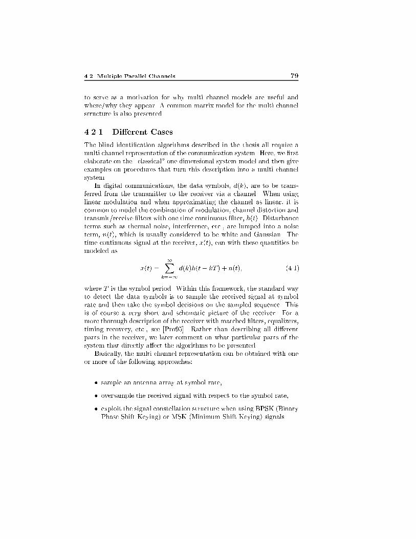
4.2 Multiple Parallel Channels 79
to serve as a motivation for why multi channel models are useful and
where/why they appear. A common matrix model for the multi channel
structure is also presented.
4.2.1 Di�erent Cases
The blind identi�cation algorithms described in the thesis all require a
multi channel representation of the communication system. Here, we �rst
elaborate on the \classical" one dimensional system model and then give
examples on procedures that turn this description into a multi channel
system.
In digital communications, the data symbols, d(k), are to be trans-
ferred from the transmitter to the receiver via a channel. When using
linear modulation and when approximating the channel as linear, it is
common to model the combination of modulation, channel distortion and
transmit/receive �lters with one time continuous �lter, h(t). Disturbance
terms such as thermal noise, interference, etc., are lumped into a noise
term, n(t), which is usually considered to be white and Gaussian. The
time continuous signal at the receiver, x(t), can with these quantities be
modeled as
x(t) =
1Xk=�1
d(k)h(t� kT ) + n(t); (4.1)
where T is the symbol period. Within this framework, the standard way
to detect the data symbols is to sample the received signal at symbol
rate and then take the symbol decisions on the sampled sequence. This
is of course a very short and schematic picture of the receiver. For a
more thorough description of the receiver with matched �lters, equalizers,
timing recovery, etc., see [Pro95]. Rather than describing all di�erent
parts in the receiver, we later comment on what particular parts of the
system that directly a�ect the algorithms to be presented.
Basically, the multi channel representation can be obtained with one
or more of the following approaches:
� sample an antenna array at symbol rate,
� oversample the received signal with respect to the symbol rate,
� exploit the signal constellation structure when using BPSK (Binary
Phase Shift Keying) or MSK (Minimum Shift Keying) signals.

80 4 Communication Systems with Multiple Channels
We will see that each of these three cases and combinations thereof give
rise to a model with the block structure depicted in Figure 4.1.
+
+
+ xL(t)
h1(t)
h2(t)
hL(t)
d(k)
...
n1(t)
n2(t)
nL(t)
x1(t)
x2(t)
Figure 4.1: A discrete time single input, multiple output communication
system. The L parallel channels, h1(t); : : : ; hL(t), may be obtained by over-
sampling, spatial sampling and/or by exploiting the signal constellation.
Antenna Arrays
Antenna arrays are used in, for example, wireless communication systems
[AMVW91]. They can amplify weak signals, provide protection against
fading, and reject interfering users [BS92, SBEM90, ZO95, Ott96]. The
case when a mobile with a single antenna transmits to a base station
equipped with an antenna array is illustrated in Figure 4.2. With an-
tenna arrays at the base station, it is obvious that the transmission from
the mobile to the base station can be modeled with L ( = number of
antenna elements ) parallel channels each described mathematically by
Equation (4.1). The channel, hi(t), from the mobile station to the ith
antenna di�ers from antenna element to antenna element. The di�erence
depends on, among other things, the antenna element spacing and the
propagation environment.
Temporal Oversampling
The signal at the transmitter is constructed by the system engineer and
can, contrary to the propagation environment, be subject to several struc-

4.2 Multiple Parallel Channels 81
35421
GSM
9876
Line of sight
Circular antenna array
Multipath
Multipath
Figure 4.2: An illustration of data transmission from a mobile equipped with
one single antenna to a base station equipped with a circular antenna array.
In some cases, there is a clear sight of the base station from the mobile and
it is said that there exists a line of sight path. In addition to line of sight,
the signal often re ects on objects in the surroundings on its way to the base
station; when several such paths are present, the signal is subject to multi path
propagation.
tural properties. One such property is that, in digital transmission, the
same pulse is transmitted every T seconds [TXK91, SP94, MDCM95]. If
the receiver �lters and samples the signal at lT , where l is an integer, the
received and sampled signal at the time instant lT is given by
x(lT ) =
1Xk=�1
d(k)h(lT � kT ) + n(lT )
=
1Xk=�1
d(k)h((l � k)T ) + n(lT ): (4.2)
If we introduce the notation h1(l) = h(lT ) for the sampled impulse re-
sponse, x1(l) = x(lT ) for the sampled received signal and n1(l) = n(lT )

82 4 Communication Systems with Multiple Channels
for the sampled noise, then (4.2) turns into
x1(l) =
1Xk=�1
d(k)h1(l � k) + n1(l): (4.3)
Note that (4.3) is a time discrete representation of the time continuous
model in (4.2). To this point, the cyclostationary structure of the commu-
nication signal, i.e., the same signal, h(t), is transmitted every T seconds,
has not been exploited. Now, assume that the receiver also samples the
signal at time instants t = lT + T=2,
x(lT + T=2) =
1Xk=�1
d(k)h(lT + T=2� kT ) + n(lT + T=2) (4.4)
=
1Xk=�1
d(k)h((l � k + 1=2)T ) + n(lT + T=2): (4.5)
If we introduce the notation h2(l) = h(lT +T=2) for the sampled impulse
response, x2(l) = x(lT+T=2) for the sampled received signal and n2(l) =
n(lT + T=2) for the sampled noise, then (4.4) turns into
x2(l) =
1Xk=�1
d(k)h2(l � k) + n2(l): (4.6)
Observe that (4.6) and (4.3) are both time discrete representations of
the same time continuous system in (4.2) but they model the system at
di�erent sample instants. In addition, even if the samples x2(l) and x1(l)
are taken at di�erent time instants, the input signals, d(k), to both the
time discrete systems are the same. This is due to the cyclostationary
structure of the communication signal. The time discrete channels, h1(l)
and h2(l), are in general di�erent. The conversion from one time contin-
ues channel impulse response to two time discrete impulse responses is
shown in Figure 4.3. It is evident that the oversampled process described
here can either be described as a nonstationary scalar valued process or
as a stationary vector valued process with one input and two outputs;
see Figure 4.1 with L = 2.
It is obvious that it is possible to sample more often than only two
times each symbol period and obtain more than two parallel communica-
tion channels. However, if the signal is oversampled too much, then the
time discrete channels, hi(k), will look very similar and the multi channel

4.2 Multiple Parallel Channels 83
1 2 3 4 5 6 7 8 91 2 3 4 5 6 7 8 9
h(t)
h1(n) h2(n)
n n
t
Even samplesOdd samples
Symboltime, T
Figure 4.3: An illustration of how the oversample procedure functions. The
time continuous impulse response, h(t), is sampled twice every symbol period,
T . These samples are used to construct the two time discrete impulse responses,
h1(n) and h2(n).
representation will not give any additional information about the channel
coe�cients. It is clearly seen in Figure 4.3 that even if the two channels,
h1(n) and h2(n), are not identical, they may look similar. The similarity
of the over sampled channels, hi(t), is small if the sample rate is less than
the Nyquist rate and high if it is close or above it.
In addition to the altered characteristics of the time discrete com-
munication channel, the properties of the additive noise processes ni(t)
are changed if the sampling rate is increased with respect to the sym-
bol period. If the sampling rate is equal to the Nyquist rate and if the
analog noise at the receiver front end is white, then ni(t) are temporally
uncorrelated as long as the receiver �lter is an ideal lowpass �lter. How-
ever, if the sampling rate is larger than the Nyquist rate, then ni(t) are
temporally correlated. Intuitively, the additional information about the
analog noise process that is obtained with oversampling is small if ni(t)
are temporally colored. It is thus possible to conclude that not only the

84 4 Communication Systems with Multiple Channels
properties of the channel but also the properties of the additive noise
limit the amount of information that is obtainable with oversampling.
However, in [CP96a, CP96b] it is shown that when the channel is
unknown, it is in fact necessary to oversample the received signal in ordernot to loose any information in the sampling procedure. This is contrary
to [For72] where it is shown that if the channel is known, then sampling
at the symbol rate yields a su�cient statistic for the detection of the
symbols.
Signal Constellation Properties
As mentioned earlier, the signal that leaves the transmitter is constructed
by the user and therefore exhibits known structure. The oversampling
approach described in the previous section is one way to exploit some
of the information in this signal. When working with communication
signals it is common practice to work with baseband equivalent signals
[Pro95]. This procedure makes the analysis independent of the carrier
frequency and results in a complex valued signal in the baseband. That
is, both h(t) and d(t) are in general complex valued quantities. Since h(t)
consists both of the modulated signal and the channel, we do not know
the particular structure of h(t). Though, it is still possible to construct
channel estimators that take the shape of the transmit and receive �lters
into account [Ced97]. Unfortunately, it is not possible to extract a multi
channel system in this way.
Here, we mention that in some special cases it is actually possi-
ble to exploit the structure in d(k) to obtain multiple parallel channels
[KSO96, LD98]. The symbols d(k) are in digital modulation drawn from a
�nite alphabet which in many cases is complex valued. However, in some
systems the alphabet is actually one dimensional, e.g., Binary Phase Shift
Keying (BPSK). When d(k) is real valued, the real valued symbol stream
is transmitted via a complex valued communication channel. Consider
the model in (4.1) when d(t) is real valued and separate the model in its
real and imaginary parts:
x1(t) = Refx(t)g =1X
k=�1
d(k) Refh(t� kT )g+Refn(t)g; (4.7)
x2(t) = Imfx(t)g =1X
k=�1
d(k) Imfh(t� kT )g+ Imfn(t)g: (4.8)

4.2 Multiple Parallel Channels 85
Note that the real valued property of d(k) is crucial to obtain the above
equation. That is, even in this case we can obtain two parallel commu-
nication channels, both with the same real valued input, d(t). We will in
Chapter 8 elaborate more on this procedure.
We have in this section given a brief description regarding methods
and scenarios where a multi channel framework is suitable. In the next
section, a common matrix framework for this model is given.
4.2.2 Common Framework { Matrix Formulation
Although the three methods presented in Section 4.2.1 obtain a multi
channel representation of a communication system in di�erent ways, the
resulting system can in all cases be described by the same vector valued
model. It is of course also possible to combine the three approaches and,
for example, oversample the outputs of an antenna array with respect to
the symbol rate. Even for combinations of the methods, the resulting
matrix system model is the same. The attention in this section is there-
fore not on how this multi channel model is obtained, but rather on how
its general structure is described by a common model.
In the sequel, it is assumed that one or more of the approaches men-
tioned in Section 4.2.1 is used to obtain the following discrete time, single
input, multiple output representation of the communication system:
x1(t) =
MXk=0
h(k)d(t� k) + n1(t); t = 1; : : : ;K: (4.9)
The vector valued quantities x1(t), h(k) and n1(t) are the received sig-
nal, the time discrete channel impulse response, and the additive noise,
respectively. The number of outputs/parallel channels is assumed to be
L and, hence, x1(t), h(k) and n1(t) are all L dimensional column vectors.
The order of the channel is M and the number of received snapshots is
K. Also, note that t is now a discrete time index. The vectors in the
above equation are
x1(t) =�x1(t) x2(t) : : : xL(t)
�T; (4.10)
h(k) =�h1(k) h2(k) : : : hL(k)
�T; (4.11)
n1(t) =�n1(t) n2(t) : : : nL(t)
�T; (4.12)
where (�)T denotes transpose. The scalar valued quantities xi(t), hi(t)
and ni(t) are the output signal, the discrete time impulse response, and

86 4 Communication Systems with Multiple Channels
the additive noise term of the ith communication channel, respectively.
The above equation is probably best explained by studying Figure 4.1,
where it is easily observed that (4.9) is just a vector counterpart of the
model in (4.1).
With the following de�nitions
H1 =�hL(0) : : : hL(M)
�
=
26664
h1(0) h1(1) : : : h1(M)
h2(0) h2(1) : : : h2(M)...
......
...
hL(0) hL(1) : : : hL(M)
37775 ; (4.13)
dM+1(t) =�d(t) : : : d(t�M)
�T; (4.14)
(4.9) can alternatively be written,
x1(t) =H1dM+1(t) + n1(t): (4.15)
We have now arrived at a system model where the snapshots of the out-
puts of all L channels at time instant t are stored in x1(t). Together with
the structure of dM+1(t) and n1(t), the matrixH1 completely determines
the communication system. However, the description in (4.13) does not
fully exploit the special temporal properties of the system. The special
temporal properties of x1(t) stem from the fact that at time instant t+1,
the input data vector dM+1(t + 1) is approximately a shifted version of
dM+1(t). All elements in dM+1(t + 1) are shifted one step downwards
in the column vector when compared to dM+1(t). The element at the
bottom of dM+1(t) is at the next time instant thrown away and a new
element enters at the top. The windowing process of the symbol se-
quence is illustrated in Figure 4.4. To fully utilize these time correlation
properties of the communication system, N vector samples are studied
simultaneously. This can be formulated algebraically:
xN (t) = HNdN+M (t) + nN (t); (4.16)

4.2 Multiple Parallel Channels 87
d(t + 6)
d5(t)
d5(t+ 1)The symbol sequence
d(t � 1) d(t) d(t + 1) d(t + 2) d(t + 3) d(t + 4) d(t + 5)
Figure 4.4: The structure of the symbol sequence. The symbol sequence,
fd(t)g, is scalar valued, but the vector sequence, fd5(t)g, is vector valued.
where
xN (t) =�xT1 (t) : : : xT1 (t�N + 1)
�T; (4.17)
nN (t) =�nT1 (t) : : : nT1 (t�N + 1)
�T; (4.18)
dM+N (t) =�d(t) : : : d(t�N �M + 1)
�T; (4.19)
HN =
26664
H1 0L�1 0L�(N�2)0L�1 H1 0L�(N�2)...
......
0L�1 0L�(N�2) H1
37775 : (4.20)
Here, 0i�j denotes an i�j matrix with zeros. The NL�(N+M) matrix
HN is block Toeplitz with N block rows and with the �rst block row equal
to [H1 0L�(N�1)]. The number of block rows, N , is called the length of
the temporal window and HN is often called the channel matrix. Using
a more compact notation (4.16) can be written
x(t) = Hd(t) + n(t): (4.21)
This notation is used extensively in the sequel of the thesis. The sub-
scripts indicating the dimension of the matrix are used only when there
is risk for confusion.
Finally, we have arrived at the multi channel model that is used
throughout this thesis. This model is also used in, e.g., [SP94]. By
interchanging rows in this model, the model used in, e.g., [MDCM95] is
obtained. The structure of the channel matrix is probably best illustrated
with a numerical example of a multi channel system. This can be found

88 4 Communication Systems with Multiple Channels
later in Chapter 5. Now, we turn our attention to the zeros of the derived
multi channel system in (4.21).
4.2.3 On Representations Using the Z-transform
The temporal matrix description of the communication system in Sec-
tion 4.2.2 provides insights on many di�erent properties of the system.
However, in some cases a description of the system using the Z-transformis more fruitful. Questions regarding identi�ability and rank of H are
examples of such cases. The thesis is written in such a way that de-
tailed knowledge of the Z-transform properties of vectors is not neces-
sary. However, the concept of common zeros is central in multi channel
identi�cation and needs to be de�ned properly. The section starts with
the one-dimensional Z-transform and then the corresponding vector no-
tations are given.
When working with one dimensional FIR-models it is common to
talk about the zeros of the channel. The zeros are closely connected with
the Z-transform of the channel impulse response. The Z-transform of
channel number i is de�ned to be
hi(z) =
1Xk=0
hi(k)z�k =
MXk=0
hi(k)z�k; (4.22)
where we have assumed that the impulse response of channel number i
is at most of order M . The zeros of channel number i are the possibly
complex valued numbers of z for which hi(z) is equal to zero. That is, if
zl is a zero of hi, then
hi(zl) = 0: (4.23)
The order of a channel is equal to the number of zeros of the channel.
Note that the same notation, h, is used for both the time domain and
Z-domain quantities. The current domain of interest is instead indicatedwith the corresponding function argument t or z.
For the L-dimensional communication system in (4.9) and (4.15), the
Z-transform is naturally de�ned according to
h(z) =
264
h1(z)...
hL(z)
375 =
1Xk=0
h(k)z�k =
MXk=0
h(k)z�k: (4.24)

4.3 Correlation Matrices { Notation 89
The properties of h(z) are closely connected with the identi�ability condi-
tions when using only the channel outputs in the identi�cation procedure.
If the L parallel communication channels do not all share a common zero,
then it is clear that
h(z) 6= 0; 8z: (4.25)
However, if all L channels have a common zero, say at zl, then
h(z) = 0; when z = zl: (4.26)
Vectors that are functions of polynomials, or in the more general case
rational functions of polynomials, span a so called one dimensional ra-
tional vector subspace. Rational polynomial vector spaces have several
strong and interesting properties [For75, Kai80] and are used in, e.g., cod-
ing theory, automatic control and system identi�cation. In [AMCG+97]
a special section is devoted to the applications of rational polynomial
subspaces in blind multi channel identi�cation.
4.3 Correlation Matrices { Notation
The blind estimation algorithms in this thesis are all concerned with the
second order output properties of the system. Hence, to establish param-
eter identi�ability for the investigated methods, the correlation matrices
of the involved stochastic processes are all that we need. However, to
investigate the performance of the algorithms, more information is occa-
sionally necessary. The de�nition of the correlation matrices are given
in this section. The necessary statistical assumptions on the stochastic
processes are given in Section 4.4.1.
It is assumed that all the correlation matrices are time invariant.
Thus, the channel matrix, H1, is assumed to be a �xed deterministic
quantity over the observation interval and the noise and data symbols are
assumed to be at least second order ergodic. That H1 is time invariant is
a reasonable assumption as long as the observation time is limited. For
example, it is fairly common to view the channel as constant under the
duration of one burst in the GSM system for mobile communications. In
cases where the channel is time varying, the algorithms presented in this
thesis must be modi�ed. The rest of this section is split in two subsections
in which the �rst elaborates on the system in (4.15) and the second on
the windowed system in (4.21).

90 4 Communication Systems with Multiple Channels
4.3.1 The Correlation Matrices for the Vector Snap-
shots
This section treats notations for the correlation matrices of the vector
valued processes de�ned in conjunction with the system model in (4.15).
For ease of reference, the equation of the L-dimensional communication
system in (4.15) is restated:
x1(t) =
MXk=0
h(k)d(t� k) + n1(t) =H1dM+1(t) + n1(t): (4.27)
Thus, in the system model above M + 1 consecutive data symbols are
collected in the vector dM+1(t). The correlation matrix of this vector is
�dd(�) = EfdM+1(t)d�
M+1(t� �)g; 8 integers �; (4.28)
where (�)� denotes complex conjugate transpose. The dimension of �dd(�)is obviouslyM+1�M+1. In addition, the assumed second order ergod-
icity of the scalar valued process d(t) certi�es that �dd(�) is a Toeplitz
matrix for all values of � . For the remaining processes, x1(t) and n1(t),
the correlation matrices are denoted by
�xx(�) = Efx1(t)x�1(t� �)g; 8 integers �; (4.29)
�nn(�) = Efn1(t)n�1(t� �)g; 8 integers �: (4.30)
Note that �xx(�) and �nn(�) are in contrast to �dd(�) not Toeplitz and
are in the general case rather unstructured. The only available structure
in these matrices stems directly from the de�nition of a correlation ma-
trix. For example, since the vector processes are assumed to be second
order ergodic, the relation
�xx(��) = ��xx(�) (4.31)
holds and is well known for this class of matrices.
4.3.2 The CorrelationMatrices in theWindowed Sys-tem
For ease of reference we repeat here the de�nition of the windowed output
vector:
xN (t) =�xT1 (t) : : : xT1 (t�N + 1)
�T: (4.32)

4.4 Assumptions Regarding the System 91
The covariance matrices associated with the windowed vectors xN (t) and
nN (t) are thus block Toeplitz by construction. The blocks of these ma-
trices are �nn(�) and �xx(�), respectively. We use the notations
Rxx(�) = EfxN (t)x�N (t� �)g; (4.33)
Rnn(�) = EfnN (t)n�N (t� �)g: (4.34)
Both the matrices in (4.33) and (4.34) are NL�NL. The block Toeplitz
structure of Rxx(�) is given by
Rxx(�)
=
26664
�xx(�) �xx(� + 1) : : : �xx(� +N � 1)
�xx(� � 1) �xx(�) : : : �xx(� +N � 2)...
. . ....
�xx(� �N + 1) : : : : : : �xx(�)
37775 : (4.35)
The block structure of Rnn(�) is similar to the block structure in Rxx(�).
The correlation matrix of the symbol vector corresponding to the
windowed system in (4.21) is simply an extension of �dd(�) and given by
Rdd(�) = EfdM+N (t)d�
M+N (t� �)g: (4.36)
The matrix Rdd(�) is of dimension M +N �M +N . Note that Rdd(�)
is Toeplitz and not block Toeplitz.
4.4 Assumptions Regarding the System
The system described in Section 4.2.2 is in this thesis subject to assump-
tions regarding the statistical properties of the stochastic processes. First,
general assumptions on the process correlations are given. These general
assumptions concern identi�ability in general, but they also concern the
possibility to use subspace methods. Then the special setup used in the
simulations in the blind estimation section of the thesis is outlined. A
paragraph at the end is devoted to the implications of the assumptions
on some of the critical parts in a practical communication systems.
4.4.1 Statistical Assumptions
In general, the scalar-valued data symbols are assumed to be circularly
complex Gaussian variables of zero mean. The assumption of Gaussian

92 4 Communication Systems with Multiple Channels
distributed data symbols should perhaps be commented on. In most
(all digital) communication systems, the data symbols are not circularly
distributed complex-valued Gaussian variables. For example, the data
symbols of a BPSK system with the two possible signal alternatives +1
and �1 are obviously neither circular nor Gaussian. However, as will
be shown in Chapter 6, the statistical analysis of the investigated class
of subspace identi�cation methods is independent of the distributions of
the data symbols. This holds for all the investigated subspace methods.
The only algorithm that explicitly makes use of the Gaussianity is the
covariance matching estimator to be presented in Chapter 9.
In most practical systems the correlation between the scalar valued
data symbols in dM+N (t) decays rapidly when the time di�erence � is
increased. It is thus justi�ed to make the assumption
�dd(�) = 0; j� j > d; (4.37)
where d is a limited scalar valued parameter which is chosen as small as
possible. For example, if the symbols d(t) are assumed to be temporally
uncorrelated, then d = M . The windowed correlation matrices Rdd(�)
may take on arbitrary structure with the only constraint that Rdd(0) is
full rank.
The additive noise in (4.15) is assumed to be circularly Gaussian dis-
tributed with zero mean. The circularity of the noise implies the relation
EfnN(t)nTN (�)g = 0; 8t; �: (4.38)
In addition, it is assumed that the noise is such that
�nn(0) = �2IL; (4.39)
Rnn(0) = �2INL: (4.40)
Similar to the data symbols, it is assumed that the covariance matrix of
the noise is zero for some large enough time lag
�nn(�) = 0; j� j > n: (4.41)
If the noise vectors are assumed to be uncorrelated in time, then n = 0.
As in most systems, the noise and the data processes are assumed
to be statistically uncorrelated. This results in the following covariance
matrices of the received vectors
Rxx(�) = EfxN (t)x�N (t� �)g = HNRdd(�)H�
N +Rnn(�); 8�: (4.42)

4.4 Assumptions Regarding the System 93
The special case of � = 0 is central and under the made assumptions we
have
Rxx(0) = HNRdd(0)H�
N+ �2INL (4.43)
or with simpli�ed notation
Rxx = HRddH� + �2I: (4.44)
4.4.2 Simulation Setup
The simulation environment used throughout the thesis is just a spe-
cial case of the data model de�ned in this chapter. The data symbols
are in all the simulations assumed to be temporally uncorrelated (possi-
bly complex valued) stochastic variables of zero mean and with variance
�2d. These data symbols are either drawn from a circular complex Gaus-
sian distribution or with equal probability from the alphabet f��d; �
dg.
Which particular distribution used in a speci�c simulation run is speci�ed
in the presentation of the simulation results in that chapter. Although
two di�erent distributions of the data symbols are used, the second order
statistics of the two distributions are the same. It is only in the higher or-
der moments that the distributions di�er from each other. The assumed
correlation properties result in the following covariance matrix for the
data vector:
Rdd(�) =EfdN+M (t)d�N+M (t� �)g
=
8>>>>>><>>>>>>:
�2d
"0�;N+M�� 0�;�
IN+M�� 0N+M��;�
#0 < � < N +M;
�2dIN+M � = 0
R�dd(��) �(N +M) < � < 0;
0 otherwise:
That is, the non zero sub-diagonal is shifted one step when � is increased
or decreased by 1. Note that although the data symbols, d(t), are tem-
porally uncorrelated, the data vectors, dN+M (t), are still temporally cor-
related. This fact is of great importance in the later analysis.
The additive and temporally white complex Gaussian noise is assumed
to be independent between the channels and equi-powered with variance

94 4 Communication Systems with Multiple Channels
�2. This gives the following structure of the noise covariance matrix:
Rnn(�) =EfnN (t)n�N (t� �)g
=
8>>>>>><>>>>>>:
�2
"0�L;NL��L 0�L;�L
INL��L 0NL��L;�L
#0 < � < N;
�2dINL � = 0
R�nn(��) �N < � < 0;
0 otherwise:
Note that the non zero sub diagonal is shifted L sub diagonals when � is
increased or decreased by 1.
It is convenient to de�ne the signal to noise ratio of the multi channel
system in the following way
SNR = 10 log10EfkH1dM+1(t)k2F g
Efkn1(t)k2F g: (4.45)
Here, k � k denotes the Frobenius norm [GvL89] of the indicated vec-
tor/matrix. The measure in (4.45) is in some sense the average signal to
noise ratio in all one dimensional channels. More explicitly, the quotient
in (4.45) is the sum of the received signal energy in all the one dimen-
sional channels divided by the sum of all the noise powers. To evaluate
the algorithms, the following measure is used,
MSE = 10 log10Efkh� hk2
Fg
khk2F
: (4.46)
Here, h is the vector containing the estimated channel coe�cients and h
contains the true channel coe�cients. Note that this measure is indepen-
dent on how the channels are scaled.
4.4.3 Connections to Practical Systems
In this section, we elaborate on some of the practical implications that
the assumptions in Section 4.4.1 result in. Speci�cally, we discuss the
e�ects of carrier frequency estimation and synchronization. The carrier
frequency estimation problem is treated �rst together with a brief de-
scription of the well known baseband equivalent of a narrowband signal.

4.4 Assumptions Regarding the System 95
Carrier Frequency Estimates
Communication systems are in general represented by their baseband
equivalents [Pro95]. In fact, the system studied in the previous sections
is assumed to be a baseband system. This representation makes use of
the fact that most communication signals are narrowband in comparison
to the carrier frequency. Narrowband time continuous signals can be
written using sinusoids in the following way
x(t) = a(t) cos(2�fct+ �(t)); (4.47)
where a(t) is the time varying amplitude, fc the carrier frequency and
�(t) the phase of the signal. Both a(t) and �(t) are so-called baseband
signals. Using simple trigonometric formulas this can alternatively be
written,
x(t) = xc(t) cos(2�fct)� xs(t) sin(2�fct); (4.48)
where xc(t) and xs(t) are assumed to be lowpass processes denoted the
sine and cosine quadrature components. The real signal in (4.48) can
also be represented with the complex signal �x(t) = xc(t) + ixs(t),
x(t) = Ref�x(t)ei 2�fctg: (4.49)
The complex signal �x(t) is denoted the lowpass equivalent of the sig-
nal x(t). If the carrier frequency is known exactly, then the quadrature
component xc(t) can be obtained from the real signal x(t) by �rst mul-
tiplicating x(t) with a cosine of frequency fc and then �ltering out the
lowpass component. If in this multiplication and �ltering procedure, the
cosine is replaced with a sinus, then the other quadrature component is
obtained. This process is illustrated in Figure 4.5. It it thus possible to
extract xs(t) and xc(t) from the received real valued signal x(t) and then
form the complex valued lowpass equivalent �x(t).
The exact carrier frequency is unknown in most practical systems,
only an estimate of it, fc, is available. Studying (4.49), it can be shown
that if we multiply with fc rather than fc in the down modulation and
�ltering process, the resulting baseband estimate, �x(t), is
�x(t) = �x(t)ei 2�(fc�fc)t: (4.50)
The estimated baseband equivalent is according to this expression a ro-
tated version of the true baseband process �x(t) and the rotation is time

96 4 Communication Systems with Multiple Channels
sin(2�fct)
LP
LP
xc(t)
�xs(t)
x(t)
cos(2�fct)
Figure 4.5: Conversion of a narrowband communication signal centered at fcto an equivalent baseband signal. The carrier frequency is mostly considered
known and the �lters as ideal lowpass �lters.
dependent. If the estimated carrier frequency is of poor quality, then
this rotation of the true baseband equivalent destroys the structure of
the input signal constellation. If properties of the input signal constel-
lation is used in the channel estimation procedure, this rotation of the
constellation must be negligible during the observation interval. That is,
2�(fc � fc)tobs � 2�
tobs � 1=(fc � fc) (4.51)
where tobs is the length of the observation interval. The subspace identi�-
cation procedures introduced in Chapters 6, 7 and Chapter 9 are accord-
ing to the identi�ability conditions presented in the next chapter insensi-
tive to errors in the carrier frequency estimate. This is an interesting and
useful property not shared with traditional identi�cation methods based
on training sequences. There is in these chapters therefore no assumption
on the quality of the carrier frequency estimate.
However, in Chapter 8, the presented methods exploit characteristics
of the input signal constellation that are sensitive to time dependent
rotations. For these methods the error in the estimate of the carrier
frequency must therefore be small enough to satisfy (4.51).

4.5 Subspace Ideas and Notations 97
Synchronization and Channel Order
It is assumed that the transmitter and receiver are synchronized well
enough so that the beginning of an information burst is known with an
accuracy better or equal to the symbol duration, T . Although estimation
of the channel still is possible with the methods presented in this thesis,
the detection of the transmitted information symbols requires synchro-
nization with this accuracy. Alternatively, a small (known) training se-
quence used only for the synchronization procedure can be transmitted
in the information burst.
In the GSM system the training sequence is used both for synchroniza-
tion and identi�cation of the communication channel. When comparing
blind estimation algorithms with traditional training based identi�ca-
tion techniques, the problem of symbol synchronization when using blind
techniques must therefore also be taken into account.
Throughout the thesis it is assumed that the maximum order of the L
communication channels is known (has been estimated correctly). This
assumption is of course not valid in practice where it in many cases is
di�cult to determine the true channel order. There exist subspace based
algorithms that include the channel order estimation process [GKO98,
PJS98]. However, for the large sample analysis performed in this thesis,
the assumption of a known channel order is reasonable.
4.5 Subspace Ideas and Notations
As mentioned earlier subspace algorithms exploit the low rank structure
of HN for the determination of the channel coe�cients. This is achieved
by dividing the column space of the received vectors into a signal and
a noise subspace. To explain how the subspace based algorithms work,
study the noiseless model of the communication system:
xN (t) = HNdN+M (t): (4.52)
In the noiseless case, the received vectors are according to this formula
exact linear combinations of the columns in HN . By collecting a number
of received vectors it is therefore possible to determine the space spanned
by the columns in HN . The space that the columns in HN spans is
indicated with spanfHNg. This space is called the signal subspace and
the space orthogonal to the signal subspace is called the noise subspace.
As will be seen in later chapters, these subspaces uniquely determine

98 4 Communication Systems with Multiple Channels
the channel matrix up to a complex scalar multiplication. It is therefore
straight forward to estimate the channel coe�cients by a least squares �t
between the space spanned by the parameterized channel and the space
spanned by the received vectors. The idea with subspace based methods
can thus be summarized in the following way,
� Study a model of the system where the parameters are uniquely
determined by the signal subspace (or equivalently the noise sub-
space). In the next chapter this is shown to hold for our model of
the multi channel communication system.
� Estimate the signal (noise) subspace from received data.
� Fit the parameterized model to the estimated subspace using a
scalar valued cost function. Suggested cost functions are given in
Chapter 6.
The �rst and second items in the list are, as indicated, explained else-
where in the thesis. In the noise free case it was argued that the subspace
can be estimated directly from received data. In the noisy case the sub-
spaces are estimated by an eigenvalue decomposition of the sample co-
variance matrix. This estimation procedure and some notation are given
next.
4.5.1 Basic Notation
One common way to describe the signal and noise subspaces is to use two
matrices that each span one of the two subspaces. In this thesis Us is
used to denote a matrix with orthogonal columns that spans the signal
subspace and the notation Un is used for the corresponding noise sub-
space quantity. As indicated above, these two matrices can be computed
from an eigenvalue decomposition of the covariance matrix,
Rxx(0) =
NLXk=1
�kuku�
k = Us�sU�
s +Un�nU�
n ; (4.53)
where
Us =�u1 u2 : : : uN+M
�; (4.54)
Un =�uN+M+1 uN+M+2 : : : uNL
�; (4.55)
�s =diag [�1; : : : ; �N+M ] ; (4.56)
�n =�2I; (4.57)

4.5 Subspace Ideas and Notations 99
and where the eigenvalues are numbered in descending order. Remember
the formula for the covariance matrix,
Rxx(0) = HNRddH�
N + �2I; (4.58)
where HN and Rdd are full rank matrices. Due to the full rank assump-
tions of Rdd(0) and HN , the �rst N +M largest eigenvalues are greater
than the noise variance and theNL�N�M smallest eigenvalues are equal
to the noise variance. Furthermore, the eigenvectors corresponding to the
N +M largest eigenvalues span the signal subspace and are columns of
Us. The eigenvectors corresponding to the smallest eigenvalues span the
noise subspace and are thus the columns of Un. The quantity �s � �2I
appears on several places in the thesis and it is therefore convenient to
introduce the notation
~� = �s � �2I: (4.59)
Sample estimates of the eigenvectors spanning the signal and noise
subspaces can be obtained from the sample covariance matrix,
Rxx =1
K �N + 1
KXt=N
xN (t)x�
N (t) = Us�sU�
s + Un�nU�
n : (4.60)
Under the assumptions on the symbol and noise sequences, the above
estimate of the covariance matrix converges both in mean square sense
and with probability one to the true covariance matrix. In addition, the
eigenvectors and the eigenvalues of the sample covariance matrix converge
to their true counterparts [JF85]. Thus, it is possible to obtain consistent
estimates of the signal and noise subspaces. Furthermore, by testing the
multiplicity of the smallest eigenvalue, the dimensions of the subspaces
may be determined from data.


Chapter 5
Parameterizations and
Identi�ability
First in this chapter, a numerical example of the linear parameterization
of the channel matrix in Chapter 4 is given. In addition, a minimal and
linear parameterization of the noise subspace is presented. Certain selec-
tion matrices are introduced which simplify the notation when minimizing
the cost function used for the identi�cation of the channel parameters.
After these two parameterizations are presented, identi�ability issues
for the system model introduced in the previous chapter are treated.
The identi�ability results can be divided into two parts. First, when is
it possible to construct an estimator of the parameters in the channel
matrix, using as inputs to the estimator only the second order statistics
of the channel outputs? This question has been intensively investigated
after the publication of one of the �rst second order based identi�cation
methods [TXK91]. The answer can be found by studying the rank of the
channel matrix. Alternatively, the relative location of the zeros in the
di�erent channels gives the same answer. After this result is clari�ed,
the next question is answered: When is it possible to uniquely identify
the channel parameters using a subspace based approach? The results
we refer to show that, using large enough temporal window lengths, these
two questions are equivalent.
The identi�ability statements presented are given for discrete time
systems and are expressed using the relative location of the zeros in the
di�erent channels. When one or more of the approaches mentioned in

102 5 Parameterizations and Identi�ability
Chapter 4 is used to obtain the multi channel discrete time representation
of the time continuous system, it is not straight forward to show when the
identi�ability conditions are satis�ed. A section is therefore devoted to a
clari�cation of some of the implications that the identi�ability conditions
result in.
5.1 Subspace Parameterizations
The system model in Chapter 4 automatically results in a linear param-
eterization of the signal subspace. It is therefore only studied brie y in
this section. A minimal linear parameterization of the noise subspace
is on the other hand more complicated to derive [Slo94]. The linear
parameterizations of the fundamental subspaces result in cost functions
that are quadratic in the channel parameters. The cost functions can
therefore be minimized analytically and no numerical search is necessary
during the identi�cation procedure. Finally, formulas for converting one
parameterization to the other are given.
5.1.1 Signal Subspace Parameterization
The linear parameterization of the signal subspace is given by the channel
matrix, HN . As seen in the previous chapter, this matrix is linearly pa-
rameterized by the channel coe�cients in the sub channels. The following
example illustrates the structure of the channel matrix.
Example 5.1. Consider the following model of a communication system
with three communication channels
x1(t) =
24 6 3 9 7
7 4 5 2
2 5 4 1
352664
d(t)
d(t� 1)
d(t� 2)
d(t� 3)
3775+ n1(t): (5.1)
Note that the channel matrix in this formulation spans the complete 3
dimensional observation space. Thus, even without noise, x1(t) is not
con�ned to a low rank vector subspace. Note, however, that in the noise
free case, x1(t) is con�ned to a low rank rational polynomial vector sub-
space. To illustrate this we use a temporal window of length N = 3 and

5.1 Subspace Parameterizations 103
obtain
x3(t) =
24 x1(t)
x1(t� 1)
x1(t� 2)
35 =
26666666666664
6 3 9 7 0 0
7 4 5 2 0 0
2 5 4 1 0 0
0 6 3 9 7 0
0 7 4 5 2 0
0 2 5 4 1 0
0 0 6 3 9 7
0 0 7 4 5 2
0 0 2 5 4 1
37777777777775d6(t) + n3(t): (5.2)
It is easily shown numerically that the channel matrix in (5.2) is full
column rank, i.e., all columns are linearly independent. The matrix spans
only six dimensions of the nine dimensional vector space. If the structure
of the noise covariance matrix is known, this subspace can be identi�ed
from data and the channel matrix can in fact be determined using a
subspace identi�cation technique.
5.1.2 A Noise Subspace Parameterization
When a linear parameterization of the signal subspace is already given
by the formulation of the problem, it may seem unnecessary to study also
linear parameterizations of the noise subspace. However, when weighting
is applied it can in some cases be advantageous to use a parameteriza-
tion of the noise subspace. This is commented on later in Chapter 6 and
Chapter 7. To arrive at a linear parameterization of the noise subspace,
we �rst give some general comments on what the structure in HN im-
plies on such a parameterization. Then, a speci�c example of a linear
parameterization found in [Slo94] is described.
The channel matrix, HN , exhibits a shifted structure; each block row
in this matrix is equal to the block row above, but it is shifted one column
(not block column) to the right. Suppose that we can �nd a row vector,
say g, that is orthogonal to HN , i.e.,
gHN = 0: (5.3)
The structure of HN implies that, if the last L elements in g are zero,
then we can construct another vector, say ~g, that is orthogonal to HN
by shifting the elements in the row vector g L steps to the right. (The L
rightmost elements in g are shifted out of the vector.) If there are more
than L tailing zeros, this process may be repeated.

104 5 Parameterizations and Identi�ability
The parameterization described in [Slo94] exploits the above men-
tioned cyclic structure and combines it with results obtained when con-
structing a linear predictor of the noise free counterpart of the process
in (4.9). From the linear predictor it is possible to �nd L � 1 linearly
independent vectors that are orthogonal to HN . These row vectors are
denoted by g1; : : : ;gL�1. To describe the exact structure of these L� 1
vectors, a complete description of the linear predictor is needed. This is
not given here but can be found in [Slo94]. However, the row vectors gicontain tailing zeros and can thus be shifted as described previously. In
addition, each gi contains one particular entry that is always equal to
one.
The number, L � 1, of noise subspace vectors is connected to the
extension of the matrix HN to HN+1 and this is brie y discussed here.
When HN is full rank, it is possible to determine the vector dM+N (t)
from xN (t) without any errors (at least in the noise free case). When
increasing N by one, HN turns into HN+1 and we add L more equa-
tions. However, we only add one more unknown signal when dN+M (t) is
increased to dN+M+1(t). This indicates that there are L � 1 equations
that are super uous each time that N is increased by one. Hence, the
left null space of HN+1 contains L� 1 more linearly independent vectors
than the left null space of HN .
It is now possible to describe a parameterization of the space orthogo-
nal to HN . Denote the L� 1 linearly independent vectors obtained from
the linear predictor by g1; : : : ;gL�1. The NL � (N +M) �NL matrix
GN that spans the complete null space of HN is given by
GN =
26666666666666664
g1...
gL�101;L g1...
...
01;L gL�101;L : : : 01;L g1...
......
...
01;L : : : 01;L g�
37777777777777775
; (5.4)
where 0 � � � L� 2 is de�ned by
� = NL� (N +M)� (L� 1) (5.5)

5.1 Subspace Parameterizations 105
and is given by
=
�NL� (M +N)
L� 1
�: (5.6)
Here, bxc indicates the largest integer less than or equal to x. That is,
we create GN in an iterative manner by shifting each of the L � 1 �rst
row vectors L steps to the right. This right shift is repeated complete
times.
Note that when L � 1 is not a factor of NL � (M + N), then an
additional \non-complete" last step is needed in order for GN to span
the complete null space of HN . For the �rst � row vectors the right shift
process is repeated + 1 times and for the last L � 1 � � vectors the
right shift process is repeated times. For notational convenience we
also introduce pi, which is the number of times that gi appears in GN .
That is, pi is either equal to or + 1.
The parameterization GN described here is equivalent to the one
found in, e.g., [Hua96], for the case of two channels. In this case, L�1 = 1,
there is thus only one vector that is shifted in GN . The subscript N on
GN indicates the size of the temporal window that is used when forming
the corresponding channel matrix HN .
The parameterization is valid if the channels are linearly indepen-
dent, that is, when H1 is full rank and if h1(M) 6= 0. To illustrate the
parameterization, an example is provided.
Example 5.2. The noise subspace of the channel matrix in (5.2) has thefollowing structure
GN =24
�0:712 0:975 �1:275 �0:331 0:657 1 0 0 0
�0:931 1:677 �3:075 �1:079 2:561 0 �0:286 1 0
0 0 0 �0:712 0:975 �1:275 �0:331 0:657 1
35 :
In this matrix, 1 and 0 are not to be considered as parameters. Noting
this, the �rst row contains 5 parameters and the second row contains 6
parameters. The last row is just a shifted version of the �rst row and no
more parameters are thus introduced in the last row. The noise subspace
corresponding to the channel matrix in the �rst example is thus parame-
terized by 11 parameters, but the channel matrix is parameterized by 12.
This is due to the fact that the channel matrix is only identi�able up to a
complex scalar multiplication by its column space. The structure of the
matrix in this example is typical for the structure of the noise subspace

106 5 Parameterizations and Identi�ability
using the minimal linear parameterization. First we have two rows, the
number of channels minus one, containing the parameters. Then the rest
of the rows in the noise subspace are just shifted versions of the �rst
ones.
5.2 Identi�ability
Identi�ability in the blind context is equal to identi�ability up to a com-
plex scalar multiplication. This because when we only observe the statis-
tics of the outputs, we can not determine the absolute strength and phase
of the input signals. This is easily seen by studying the two systems in
Figure 5.1. There, the outputs are exactly the same but the inputs and
the channels are di�erent up to a complex scalar multiplication. Studying
x(t)
h(t)
h(t)=c
d(t)
c � d(t)
x(t)
Figure 5.1: Two di�erent communication channels with identical outputs.
Observing only the output, the scalar valued multiplication of the channel can
not be determined.
the outputs of the systems in Figure 5.1 the problem with the scaling is
obvious.
Practically, the parameters must be strictly identi�able from the data
and in order to obtain strict identi�ability the parameter set must be
constrained in some way. The two most common restrictions of the pa-
rameters are linear and norm constraints. The linear constraints used in
this thesis are given in the section describing the signal and noise sub-
space parameterizations. Also, note that the theorems in this section
are derived and proved under assumptions of a noise less system. This
seems restricting at a �rst glance, but the subspace identi�cation results
presented at the end of the section reveals that the results are valid also
for systems with additive white noise.
5.2 Identi�ability 107
5.2.1 General Results
The general identi�ability results are expressed using channel matrices,
HN , obtained from the same communication system, H1, but with dif-
ferent sizes of the temporal windows, N . As mentioned before, the iden-
ti�ability issues have been extensively investigated and due to this we
only refer to well known articles for the proofs. The following theorem
summarizes the results of the general identi�ability conditions using only
second order statistics [TXK93, TXK91, Tug95],
Theorem 5.1. First, assume that at least one communication channelis of order M , that is h(0) 6= 0 and h(M) 6= 0. In addition, assume thatthe signal sequence d(k) is persistently exciting of order 2M +1 and thatthe following two equivalent conditions hold,
� HM is full column rank, that is, the columns are linearly indepen-dent,
� no zero is shared by all communication channels,
then, in the noise free case, the channel matrix is uniquely identi�able upto a complex scalar multiplication using only the second order statistics.
Note that the identi�ability results can be found either by studying
the rank ofHM or by studying the location of the zeros. For a de�nition of
persistence of excitation of stochastic processes see, e.g., [Lju87]. Now we
know that as soon as HM is full rank, then, using a method that exploits
all available information in the second order statistics, it is possible to
identify the system uniquely. An example of such an estimator is the
covariance matching estimator described in Chapter 9. It now remains
to prove that the same holds for subspace based estimators.
5.2.2 Subspace Results
The question is whether or not it is possible to determine a unique channel
matrix knowing only the column space it spans. The following theorem,
�rst proved in [MDCM95], gives the answer:
Theorem 5.2. If N > M then, under the conditions of Theorem 5.1,HN�1 is guaranteed to be full column rank. In addition, HN is iden-ti�able up to a complex scalar multiplication from the column space itspans.

108 5 Parameterizations and Identi�ability
Thus, if HN�1 is full column rank, then the channel coe�cients in
HN can be estimated using a subspace based technique. Using the �rst
theorem in this section, we conclude that if the system is identi�able
from the second order statistics (using no a priori information about the
phase of the system), it is also possible to identify the system using a
subspace technique. However, the temporal window length, N , must be
chosen larger than M to guarantee identi�ability. So, if we choose the
temporal window length larger than or equal to M + 1, identi�ability is
guaranteed for a subspace method as long as the system is identi�able
from the second order statistics only.
Now, what happens when additive white noise is present? As indi-
cated before, the system is still identi�able. This is true because when
the channel matrix is low rank, the noise covariance can be determined
by studying the smallest singular values of the covariance matrix. Af-
ter that it is only to subtract the noise covariance matrix, �2I, and we
are back to a noise less system. A number of di�erent subspace based
techniques, relying on one or both of these theorems, have been studied
since the �rst publication [TXK91]; see, e.g., [Slo94, MDCM95, XLTK95,
KO96, KO98c].
5.3 Identi�ability Implications
The identi�ability results in the previous section are given for time dis-
crete systems and formulated using the concept of zeros. The question is
whether multi channel communication systems obtained with temporal
oversampling, spatial sampling or signal exploitation lack common zeros.
It is obvious that not all the derived multi channel systems lack common
zeros and it is therefore important to examine if at least most multi chan-
nel representations obtained with one of the three suggested approaches,
or combinations thereof, lack common zeros. Few experiments have been
performed on real data sets, but the results in [GKOY97] obtained on
data sets collected from an experimental PHS system ( Personal Handy-
phone System), give some hints of the potential/limits of the methods.
Both spatial as well as temporal over sampling is in this contribution
investigated using blind methods based only on the second order statis-
tics. The results indicate, as expected, that temporal over sampling and
spatial sampling should be combined.
First in this section, temporal oversampling with respect to the sym-
bol period is discussed and then spatial sampling is commented on.

5.3 Identi�ability Implications 109
5.3.1 Temporal Oversampling
Consider the case when the multi channel representation is obtained using
over sampling of a single communication channel. How are the identi-
�ability conditions transfered from the time discrete representation to
the time continuous channel? That is, what time continuous channels
can be identi�ed using temporal over sampling only? This question is
not straight forward to answer, but here some nontrivial examples of
time continuous channels are given that are unidenti�able using only the
second order statistics.
In [Tug95] the author points out that time continuous channels with
delays that are all multiples of the symbol period, T , are unidenti�able
from the second order statistics. In [Din96] this class of oversampled
channels unidenti�able from second order statistics is enlarged with three
more cases.
The problem with loss of identi�ability for certain classes of channels
leads to robustness problems. Even if the channel is identi�able, but
it is close to a non-identi�able class of channels, ill conditioning of the
identi�cation procedure is expected. The robustness issue is discussed in,
for example, [EAJT96]. The literature suggests that from a robustness
point of view, oversampling should be combined with other methods, e.g.,
spatial sampling, �nite alphabet properties.
5.3.2 Spatial Oversampling
Using spatial sampling seems to be an interesting solution to the problems
that arise when using temporal oversampling only. In wireless commu-
nications the signal is in many cases transmitted from a mobile using a
single antenna to a base station using multiple antennas. A widely used
assumption is that when specular multipaths are present, the di�erent
physical channels are uncorrelated. If this is the case, it is reasonable to
assume that when the number of antenna elements is large, then no zero
is shared by all channels; see Figure 5.2.
However, if the transmit and the receive �lters are included in the
channel model, then the multi channel system is in practice given by the
scheme in Figure 5.3. All parallell communication channels will thus in-
clude the same transmite and receive �lters. However, as pointed out in
[RPP97], using a combined temporal and spatial approach will in gen-
eral result in a system without common zeros. Except for the combined
temporal and spatial sampling, another possible approach to deal with

110 5 Parameterizations and Identi�ability
...
h1(t)
h2(t)
hL(t)
Mobile station
Base station
antenna array
...
Figure 5.2: Approximately uncorrelated physical channels, h1(t); : : : ; hL(t),
between transmitter and receiver.
......
...
d(t)
~d(t)g(t)
g(t)
g(t)
h1(t)
h2(t)
hL(t)
x1(t)
x2(t)
xL(t)
Figure 5.3: Model of a spatially sampled communication system with trans-
mit and receive �lters included. The e�ect of transmit and receive �lters is
modeled by the common �lter g(t) and the physical channels are denoted hi(t).
In certain environments the physical channels, hi(t), can be modeled as sta-
tistically independent. This indicates that common zeros will in general not
appear among hi(t).

5.4 Selection Matrices 111
common zeros is to identify only the physical channel and neglect the
transmit and recieve �lters. In that case ~d(t) in Figure 5.3 can be seen
as the input to the physical multi channel system to be identi�ed. The
identi�cation methods presented in later chapters will theoretically work
with this approach as long as the orders of the physical channel and
transmit/receive �lters are estimated correctly. In practice, a non trivial
detection of channel orders must be developed.
In this thesis, no suggestions are given for how to solve the problem
with transmit and receive �lters. However, it is important to keep in
mind that these problems will certainly in uence the performance of the
identi�cation algorithms when applied to real data sets. The theoret-
ical analysis performed in the thesis gives a hint on how sensitive the
identi�cation is with respect to common zeros.
5.4 Selection Matrices
From a notational point of view it is practical to de�ne two selection
matrices for both parameterizations. These selection matrices are useful
when working with the estimators and the weightings introduced in later
chapters. In addition, the selection matrices can be used to relate the
two parameterizations of the noise and signal subspace.
5.4.1 Linear Relations
According to the identi�ability results, HN is only identi�able up to a
complex scalar multiplication from the second order statistics. To avoid
problems in the estimation procedure due to this ambiguity, one param-
eter in HN is �xed to a prede�ned value, say to c. For ease of notation,
the rest of the complex valued parameters in HN are collected in an
(M + 1)L � 1 column vector denoted hc. In the subspace estimation
process to be described, the following relation between H and hc is used
extensively,
vec[HN ] = �hhc + �h: (5.7)
Here, vec[�] is the vectorization operator de�ned in, e.g., [Bre78, Gra81]
and �h is a selection matrix containing only zeros and ones. The last
vector in the above equation, �h, contains zeros and the �xed complex
parameter c. At one speci�c point in the thesis we will also need the

112 5 Parameterizations and Identi�ability
relation and de�nitions in
vec[HT
N ] =~�hhc + ~�h: (5.8)
The notational convention in (5.7) and (5.8) is similar. It is also useful
to de�ne a real valued vector, h, containing the real and imaginary parts
of the complex valued parameters,
h =�RefhcgT ImfhcgT
�T: (5.9)
Following the notational convention used for the signal subspace param-
eterization, the complex valued parameters in GN are collected in the
(M + 1)L � 1 column vector gc. The relation between GN and gc is
given by
vec[GN ] = �ggc + �g; (5.10)
where �g is a selection matrix containing only zeros and ones. The last
vector in the above equation, �g, contains only zeros and ones, compare
with the example in Section 5.1.1. The real valued parameter vector, g,
corresponding to gc is de�ned in the same way as h.
5.4.2 Transformations Between the Parameterizations
In a communication system, the hc parameters in the channel matrix are
often more interesting than the noise subspace parameters collected in
gc. Therefore, we present the one to one non linear mapping between
these two parameters. Given this transformation it is also possible to
transform a covariance in the estimated gc parameters to a corresponding
covariance in the estimated hc parameters. The transformations between
the complex valued parameters are given by the following expressions
hc =�h�T
h (IN+M G�NGN )�h
i�1
�T
h (IN+M G�NGN )�h; (5.11)
gc =�h�T
g(Hc
NHT
N INL�N�M)�g
i�1
�T
g(Hc
NHT
N IN+M )�
g;
(5.12)
where the derivation of these expression is given in Appendix C.1. The
large sample covariance matrix of g can be transformed to a covariance
matrix of h with the following expression,
�h = T�gTT ; (5.13)
where �g is the covariance matrix of g and �h is the covariance matrix of
h. An expression for T and a proof of (5.13) are given in Appendix C.1.

Chapter 6
Weighted Subspace
Identi�cation
In this chapter, the subspace formulation is used to derive two asymp-totically best consistent channel estimators within the class of subspace
based algorithms. They both exploit the orthogonality property between
the noise and the signal subspace. The �rst approach is based on the nat-
ural linear parameterization of the signal subspace and the second on the
minimal linear parameterization of the noise subspace presented in Chap-
ter 5. The estimates are in both cases computed in a two step Markov-like
procedure. Estimates computed by using the signal subspace parameter-
ization are obtained by optimal weighting of the unweighted method �rst
presented in [MDCM95]. Estimates using the noise subspace parameter-
ization are obtained in a similar manner.
The analysis performed in this chapter results in closed form expres-
sions for the estimation error covariance matrix for both parameteriza-
tions and for general weighting matrices. For the special case of identity
weighting the theoretical results for the signal subspace parameteriza-
tion coincide with the results in [QH96, AMCG+97]. In the optimally
weighted case they give the lower bound on the estimation error covari-
ance matrix that is attainable within the class of subspace based estima-
tors. The algorithms produce asymptotically optimally unbiased param-
eter estimates, hopt, in the sense that in large samples
Covariance(hopt) � Covariance(h); (6.1)

114 6 Weighted Subspace Identi�cation
holds for all h that are obtained with a subspace based technique. The
notation in (6.1) means that Covariance(h)�Covariance(hopt) is a pos-
itive semi de�nite matrix.
The statistical analysis of the methods is based on ideas found in
[ESS94]. However, here the statistical assumptions are di�erent and the
covariance matrices for both the signal and the noise components of the
received signal are allowed to be fairly general. The statistical results
are presented with as general assumptions as possible on the underlying
stochastic processes. They are thus applicable to a large class of subspace
identi�cation algorithms and not restricted to this blind identi�cation
framework only. To illustrate this, the cost function for the weighted
subspace �tting algorithm (WSF) in sensor array processing is established
using the expressions derived in this chapter.
The disposition of the chapter is as follows. First, a review of two
early subspace based methods is given. Then, a section follows in which
the weighted subspace approach for both the signal and noise subspace
parameterizations is described. The statistical analysis is presented in
Section 6.3 followed by the derivation of the WSF cost function. In the
last sections, simulation results are presented and conclusions are drawn.
6.1 Early Methods
After all the system models and the identi�ability results in Chapters 4
and 5, brief descriptions of two of the early methods within second order
based identi�cation are given herein. For those readers that are unfamil-
iar with second order based methods, this section serves as an introduc-
tion to the investigated estimator. A more complete review of several
methods suggested for blind second order based identi�cation can be
found in, e.g., [LXTK96, TP98].
6.1.1 A First Suggestion
One of the �rst papers where only the second order statistics of the
channel outputs is used to identify the channel coe�cients is written by
Tong [TXK91]. The algorithm suggested by Tong et. al. only works for
uncorrelated input signals. The algorithm exploits the fact that, in the
noise free case, it is possible to identify the channel matrix up to a unitary
rotation from the signal subspace of the covariance matrix
Rxx(0) = HNRdd(0)H�
N = �2dHNH�
N : (6.2)

6.1 Early Methods 115
Here, the assumption that the symbols are uncorrelated (Rdd(0) = �2dI)
is exploited in the second equality. If we use the standard notation Us
for the matrix that contains the singular vectors that span the signal
subspace then the relation between Us and the channel matrix is
HN = UsT (6.3)
Here, T is a square and unitary matrix. For unique determination of HN
it remains to determine T. In the paper, the authors suggest to study
the covariance matrix at time lag 1
Rxx(1) = HNRdd(1)H�
N= �2
dHNDH
�
N; (6.4)
where D is a matrix with zeros everywhere except for the elements in the
diagonal below the main diagonal which are all ones. If we multiply with
U�s both from the left and the right we obtain
U�sRxx(1)Us = TDT�: (6.5)
Since T is a unitary matrix, multiplication from the left yields
U�sRxx(1)UsT = TD: (6.6)
In this last equation all quantities are known (or can be estimated from
data) except for T. To continue, denote the column vectors in T with
t1; : : : ; tN+M . With this notation the above equation yields
U�sRxx(1)Ustk =
(tk+1; k � N +M � 1
0; k = N +M(6.7)
This relation identi�es tN+M up to a complex scalar multiplication and
then all other vectors in T can be determined recursively up to the same
scalar multiplication.
It is now possible to outline a procedure to estimate the matrix HN
from the received data vectors.
1. Estimate Rxx(0) and Rxx(1) from the received data vectors. Com-
pute an estimate of Us.
2. Determine T from (6.7).
3. Compute HN from (6.3).

116 6 Weighted Subspace Identi�cation
Although the above algorithm constituted a major breakthrough, it has
several drawbacks. First, the channel matrix HN is determined using
an unstructured approach, that is, the information that we \know" that
certain entries in HN are zero is not used. Second, even in the noise
free case the method does not give exact answers to the problem. This
because it takes some time before the sample estimate of the covariance
matrix converges to the true value, i.e., the method is not high SNR
e�cient.
To deal with the high SNR ine�ciency, another algorithm was sug-
gested by Moulines [MDCM95]. This algorithm exploits the orthogonal-
ity property between the noise and the signal subspace for the identi�ca-
tion of the channel coe�cients in HN . As indicated by the identi�ability
conditions in the previous chapter, this property determines the channel
coe�cients up to a complex scalar multiplication. The parameters are
thus estimated according to
hc = argminhkU�
nHNk2F : (6.8)
This method exhibits some advantages in comparison to the approach
proposed by Tong et. al.. The method suggested by Moulines et. al.
is high SNR e�cient and it is a parameterized method that exploits
the structure present in the channel matrix HN . Also, as long as the
covariance matrix of the symbol vector is full rank, the second order
properties of the symbols are not critical. The symbols can thus be
temporally dependent and the identi�cation method will still yield the
true channel coe�cients.
This chapter contains a detailed investigation of the second approach
in this section. The asymptotical properties of the estimates are deter-
mined as well as the optimal weighting matrices to use when the cost
function is formed.
6.2 Estimation Procedure
Herein, the weighted estimation procedure is presented. The parameter
estimates are obtained as the minimizing arguments of a weighted least
squares �t. Once the eigenvalue decomposition of the sample covariance
matrix is computed, these estimates can due to the linear parameteriza-
tion of both subspaces be solved for analytically. This results in closed
form solutions for the parameter estimates. As mentioned in the in-
troduction, the least squares �t is based on the orthogonality property

6.2 Estimation Procedure 117
between the signal and noise subspace. Note that according to the iden-
ti�ability results in Theorem 5.2, this property uniquely speci�es both
parameterizations (possibly up to a complex scalar multiplication).
6.2.1 Signal Subspace Parameterization
Below, an asymptotically optimally weighted version of the approach
presented in [MDCM95] is introduced. The algorithm exploits the or-
thogonality property between the noise subspace and the channel matrix
UnU�
nHN = 0: (6.9)
The projection matrix UnU�
nis used here rather than only Un in order
to guarantee unique convergence in large samples when replacing UnU�
n
with UnU�
n. Since Un spans a degenerate subspace (the NL �N �M
smallest eigenvalues are equal), Un is not guaranteed to converge to a
well de�ned quantity. However, UnU�
nwill converge to UnU
�
nin large
samples. Since the analysis of the methods assumes that the convergence
is well de�ned, we choose to work with UnU�
n throughout the chapter.
When the noise subspace is estimated from received data, the noise
subspace and the channel matrix are only approximately orthogonal, i.e.,
vechUnU
�
nHN
i= �s; (6.10)
where �s is the residual vector. Note that if �s is not circularly dis-
tributed, it is necessary to separate the above equation into real and
imaginary parts when its covariance matrix is considered. If the correla-
tion between the real and imaginary parts is neglected, then the weighted
approach is not guaranteed to be optimal within the class of subspace
based estimators relying on the orthogonality property. Later it is shown
that �s is if fact not circularly distributed and it is thus necessary to take
the correlation into account. This observation is one distinction between
this contribution and the results reported in [AMCG+97, MCGL96].
With one channel parameter �xed and after the cost function has been
separated into its real and imaginary parts, we can rewrite (6.10) on the
following form
sh+ s =
��rs
�is
�; (6.11)
where h is a real 2(M+1)L�2 dimensional column vector containing the
channel parameters and with the �xed complex parameter removed; see

118 6 Weighted Subspace Identi�cation
further Section 5.4. The real and imaginary parts of �s are denoted �rsand
�is, respectively. Expressions for s and s are given in Appendix C.2.
The optimal estimate within the class of subspace based algorithms is
obtained by:
h = argminh(sh+ s
)TWs(sh+ s); (6.12)
where the symmetric weighting matrixWs � 0 is chosen as the inverse of
the residual covariance matrix. If this inverse does not exist, then proper
use of the Moore-Penrose pseudo inverse [BIG73] results in optimal esti-
mates. Minimizing the cost function in (6.12) with respect to h results
in the estimated channel coe�cients
h = �(T
sWss)�1
T
sWs s: (6.13)
A discussion on the choice of an optimal weighting matrix in this pro-
cedure is found in Section 6.3. Note that with Ws = I and with the
constraint that one parameter is �xed, (6.13) coincides with the algo-
rithm in [MDCM95].
6.2.2 Noise Subspace Parameterization
The estimation procedure that is used to determine the parameters in
GN , using the orthogonality property, is similar to the one using the
signal subspace parameterization in the previous section. With estimates
of the signal subspace the orthogonality property yields
vechGNUs
i= �n: (6.14)
The statistical properties of the residual vector make it necessary to sep-
arate also this expression into real and imaginary parts to guarantee
optimal performance when weighting is applied. This results in the ex-
pression
ng + n =
��rn
�in
�: (6.15)
Expressions for n and nare given in Appendix C.2 and g is a real
valued 2(M + 1)L� 2 dimensional column vector containing the param-
eters in GN ; see further Section 5.4. Following the same procedure as in

6.3 Statistical Analysis 119
the signal subspace parameterization we use the standard quadratic cost
function
g = argming(ng + n)
TWn(ng + n); (6.16)
whereWn � 0 is a symmetric matrix to be determined. Minimization of
this cost function with respect to g gives the following estimates of the
parameters in GN ,
g = �(T
nWnn)�1
T
nWn n: (6.17)
Next, optimal weighting matrices as well as the asymptotical covariance
matrix of the asymptotical distribution of the parameter estimates are
determined.
6.3 Statistical Analysis
In order to determine the optimal asymptotic weighting matrices it is
necessary to determine the covariance matrix of the residual. The knowl-
edge of these statistics also gives the covariance matrix of the parameter
estimates via standard formulas found in, e.g., [SS89, Por94].
Below, the results are collected in theorems and the corresponding
proofs are placed in the appendices. The derivations hold for signal co-
variance matrices and for noise covariance structures restricted to the
model in Chapter 4. To enable the use of these expressions in other
application areas, the theorems are formulated as general as possible.
6.3.1 The Residual Covariance Matrices
The derivation of the residual error covariance is inspired by the approach
in [ESS94, CTQ89]. The key idea is to relate the large sample properties
of Us and UnU�
nto the properties of the sample covariance estimate
Rxx(0). When the additive noise is Gaussian, the large sample properties
of the estimated sample covariance matrix are then easily calculated.
Because of the separation of the original system into real and imagi-
nary parts, the following expected values are to be determined for both
parameterizations
�� = limK!1
K Ef���g; (6.18)
~� = limK!1
K Ef��T g: (6.19)

120 6 Weighted Subspace Identi�cation
Here, � denotes the complex valued residual in either the noise or the
signal subspace approach. We will occasionally denote �� and ~� with the
\circular" and \non-circular" covariance matrix, respectively. In the case
of the signal subspace parameterization method, the above quantities are
indexed with s, i.e., ��s and ~�s, and in the noise subspace parameteriza-
tion with n. With knowledge of these covariance matrices, the covariance
matrix of the real valued residual is easily found according to
� =1
2
"Ref ��g+Ref ~�g
�Imf ��g+ Imf ~�g
�TImf ��g+ Imf ~�g Ref ��g �Ref ~�g
#: (6.20)
The covariance matrix for the real valued residual is thus denoted �s
for the signal subspace parameterization and �n for the noise subspace
parameterization. A matrix expression for �� is provided by the following
theorem,
Theorem 6.1. Assume that the row space of GN is orthogonal to thecolumn space of Us and that the column space of HN is orthogonal to thecolumn space of Un, i.e., GNUs = 0 and U�
nHN = 0. If, in addition,
the complex Gaussian noise vectors satisfy the statistical assumptions inChapter 4, then
��n = limK!1
K Ef�n��ng =N�1X
�=�N+1
(��Rxx(�)�)c GNRnn(�)G
�
N
��s = limK!1
K Ef�s��
sg
=
N�1X�=�N+1
(H�NUs��Rxx(�)�U
�
sHN)c UnU
�
nRnn(�)UnU�
n
Here the de�nition � = Us(�s � �2IN+M )�1 is used and (�)c denotes
complex conjugate.
Proof. See Appendix C.3.
Remember that denotes the Kronecker product [Bre78, Gra81]. For
the second order statistics of the real valued residuals to be completely
speci�ed, it remains to determine ~�.
Theorem 6.2. Assume that the row space of GN is orthogonal to thecolumn space of HN (or equivalently Us). In addition, assume that the

6.3 Statistical Analysis 121
complex Gaussian noise vectors satisfy the assumptions in Chapter 4,then
~�n = limK!1
K Ef�n�T
ng = (�T GN )��(�GT
N)
~�s = limK!1
K Ef�s�Ts g
=�HT
NUc
s�T UnUn�
����HT
NUc
s�T UnU
�
n
�TAn expression for �� can be found in Appendix C.4.
Proof. See Appendix C.4.
Note that no assumption is made of the distribution of d(t). The
asymptotic expressions are thus valid for general distributions and deter-
ministic symbol vectors. Hence, the symbol vectors can be real valued as
in the BPSK signaling case or complex valued as in, e.g., QPSK.
For most practical cases, �� is a function of �2n, but ~� is a function
of �4n. Thus, if the signal to noise ratio is large, it is not necessary to
separate the cost function into real and imaginary parts. In applications
where the underlying system limits the number of accessible samples
for the identi�cation, a reasonable signal to noise ratio is needed if the
identi�cation is to be successful. In these cases it is not necessary to
take the correlation between real and imaginary parts into account. In
Chapter 7 we further investigate the performance of an estimator where
the non-circularity of the residual is neglected.
6.3.2 The Parameter Covariance Matrix
A problem when using the orthogonality property for blind channel iden-
ti�cation is that the residual covariance matrix will in general not be full
rank. This singularity is due to
� using UnU�
ninstead of Un in the signal subspace parameterization,
� the window procedure used to obtain a low rank model.
First, note that UnU�
nis a rank de�cient matrix by construction. The
expressions for ��s and ~�s in Theorems 6.1 and 6.2 thus show that the
residual covariance matrix is singular in the signal subspace parameteri-
zation. However, in the noise subspace parameterization only Us is used
and the same reasoning does not hold in this case. In addition, the noise

122 6 Weighted Subspace Identi�cation
subspace parameterization GN is a full rank matrix spanning the com-
plete null space. The rank de�ciency of the residual covariance matrix
is thus not due to a rank de�cient parameterization, which would have
been the case if the parameterization in, e.g., [Hua96] had been used in
the general case.
The low rank property of the residual covariance matrix is in this
case due to the window procedure which results in the block Toeplitz
covariance matrix of the received snapshots. The same block element in
Rxx(0) will appear more than once. When calculating the covariance of
vec[Rxx(0)] this covariance matrix will therefore be low rank; see, e.g.,
[KO97, KO98b] and Chapter 7. Note that if there was no temporal de-
pendence between the windowed received data vectors, then the residual
covariance matrix would be full rank. This corresponds to the case when
a model like (4.16) is obtained without the window procedure.
When the residual covariance matrix is rank de�cient, care must
be taken when calculating the optimal weighting matrix. The optimal
weighting matrix to be chosen here is optimal with respect to the es-
timation error covariance matrix of the parameter estimates. However,
the rank de�ciency is still a problem because the rank of the covariance
matrix must in practice be determined. Furthermore, the rank of the
residual covariance matrix may very well be parameter dependent in the
general case; see, e.g., Chapter 3 and Chapter 7.
If the residual covariance is full rank, then it is well known that the
optimal weighting matrix is given by its inverse. However, in the general
case when the covariance matrix is not full rank, the weighting matrix
has to be modi�ed to give the asymptotically best consistent estimates.
Theory regarding how this can be done is presented in for example [RM71,
SS89]. Combining [SS89, Sections C4.3 and C4.4], an optimal asymptotic
weighting matrix is found to be
W = (�+T )y; (6.21)
where (�)y denotes the Moore-Penrose pseudo inverse [RM71]. Note that
this is not always the only weighting matrix that gives asymptotically
best consistent estimates. If, for example,
spanfg � spanf�g (6.22)
holds, then the last term in the weighting matrix can be set to zero
without a�ecting the result. In Chapter 7 this matter is discussed in
detail and it is also shown that the span relation in (6.22) actually holds.

6.3 Statistical Analysis 123
For now, we neglect this fact and proceed with the general approach not
based on the span relation in (6.22).
The following theorem now summarizes the properties of the esti-
mates:
Theorem 6.3. Assume that the estimates of the parameters h and g
for the two methods are obtained using (6.12) and (6.16), respectively,possibly using a weighted approach. Then the parameter estimates areasymptotically unbiased and Gaussian distributed with covariance matri-ces,
limK!1
K En(h� h) (�)T
o= (T
sW
s
s)�1T
sW
s�sW
s
s(T
sW
s
s)�1;
limK!1
K En(g � g) (�)T
o= (T
nW
n
n)�1T
nW
n�nW
n
n(T
nW
n
n)�1;
where W(�) is the (possibly) parameter dependent weighting matrix.
Proof. The theorem follows from Appendix C4.3 and Appendix C4.4 in
[SS89].
If weighting is not used, then replacingW with the identity matrix of the
same dimensions gives the corresponding parameter covariance matrices.
If a weighted method is used, then the following well known two step
procedure results in asymptotically optimal estimates [SS89]:
� Estimate the parameters consistently with identity weighting ) h
(or g).
� Calculate a second estimate^h (or ^g) using the weighting matrix in
(6.21) which depends on h or g.
In the simulation section we will consider identity weighting (W = I)
and optimal weighting. Care must be taken when implementing the
weighted methods so that the correct rank of the weighting matrix is
chosen. Alternatively, the weighting matrix in (6.21) can be regularized
with a scaled identity matrix. The simulation results presented in this
chapter are obtained with the regularized approach. After the regular-
ization a standard inverse can be used instead of the pseudo inverse. The
regularized weighting matrix results in a more well behaved optimization

124 6 Weighted Subspace Identi�cation
problem and has minor in uence on the accuracy of the estimates. The
theoretical expressions for the asymptotic covariance matrix are of course
implemented without regularization.
6.4 Special Case { Direction Estimation
The formulas for the weighting matrices and the estimation error covari-
ance matrices are presented in a very general way but are also rather
complicated. To illustrate the usefulness of the expressions in other ar-
eas than blind identi�cation, the formulas are here applied to direction of
arrival estimation in sensor array processing. Speci�cally, we study the
estimation of parameters in a linear parameterization of the noise sub-
space. The less complicated covariance structure of the signal and noise
components in the received signal results in an optimal weighting matrix
which is full rank.
Assume that m signals are impinging on a uniform linear array with
L sensors. The received signals are thus given by the standard model
x(t) = A(�)d(t) + n(t); (6.23)
where d(t) is the signal vector and n(t) is additive white Gaussian noise.
This model is described in detail in Chapter 2 but is here brie y reviewed
for ease of reference. The array manifold is for the special case of a linear
array given by
A(�) =
2666664
1 1 : : : 1
ei �1 ei �2 : : : ei �m
ei 2�1 ei 2�2 : : : ei 2�m
......
...
ei(L�1)�1 ei(L�1)�2 : : : ei(L�1)�m
3777775 ; (6.24)
where � = [ �1 �2 : : : �m ]T is a vector with the direction of arrivals
of the m impinging signals. It is assumed that the signal and noise
processes are of zero mean and with covariance matrices
Rdd(�) = Efd(t)d�(t� �)g = Rdd�(�); (6.25)
Rnn(�) = Efn(t)n�(t� �)g = �2I�(�); (6.26)
where �(�) is the Kronecker delta. If in addition the noise and signals are
uncorrelated, then the covariance matrix of the received vectors is given

6.5 Simulation Examples 125
by
Rxx(�) = Efx(t)x�(t� �)g = �A (�)RddA
� (�) + �2I��(�): (6.27)
Remember that a linear parameterization of the complete orthogonal
subspace to A(�) is given by the matrix B(b) in (2.11). The subspace
based estimator can with these notations be written
b = argminb2C
vec�[B�Us]W vec[B�Us]; (6.28)
where W is a weighting matrix to be determined. Theorem 6.1 results
in:
W�1 =X�
(��Rxx(�)�)c B�Rnn(�)B (6.29)
=(��Rxx�)c �2B�B = �2�s(�s � �2I)�2 B�B: (6.30)
In the second step of a two step procedure, an estimate of the noise sub-
space parameterization, B, is available. Replacing the weighting matrix
with an estimate thereof results in
b =argminb2C
vec�[BUs]
���1
s
��s � �2I
�2 (B�B)�1
�vec[BUs]
=argminb2C
TrfB(B�B)�1B�Us(�s � �2nI)2��1
s U�sg: (6.31)
This is the well known weighted subspace �tting criterion [VO91, OVSN93]
or the MODE cost function [SS90]. The \only" property that di�ers be-
tween this array processing case and the blind identi�cation problem is
the covariance structure of the received signals. Now we return to the
blind identi�cation and evaluate the �nite sample behavior of the sug-
gested estimation methods.
6.5 Simulation Examples
To illustrate the properties of the identi�cation methods, some simulation
results and numerical comparisons are presented in this section. The
simulation setup described in Chapter 4 is used in all simulation runs.
De�nitions of signal to noise ratios and covariances are also found in that
chapter. When comparing simulation results with theoretical expressions,
the expectation operator in (4.46) is replaced with the average value over
all simulation runs.

126 6 Weighted Subspace Identi�cation
The data symbols are in all simulation examples temporally uncorre-
lated stochastic variables drawn with equal probability from the alphabet
f�1;+1g. Note that using Gaussian distributed signals instead of BPSK
signals theoretically results in the same asymptotical parameter covari-
ance. The additive complex valued noise in each channel is a temporally
white Gaussian noise process which in addition is uncorrelated among
the channels. These assumptions on the noise and the signal speci�es the
data and noise covariance matrices for all time lags.
Throughout this section, a two channel system is considered. The Z-transform representation of the FIR channels in this system is generated
by choosing di�erent values of �i in the formula
hi(z) = 1� 2 cos(�i)z�1 + z�2: (6.32)
That is, the zeros of the channel are located on the unit circle at angles
��i. In Figure 6.1 the frequency response of this FIR channel is shown
for two di�erent angles �i. The identi�ability results state that if there
are one or more zeros common to all communication channels, then the
channel parameters are not identi�able from the second order statistics.
Changing the parameter � makes it possible to study identi�cation of
parameters close to the point where the parameters become non identi-
�able. In these cases it is expected that, at least theoretically, weighting
improves the estimates considerably.
The theoretical expressions for the signal subspace parameterization
are evaluated �rst using the values �1 = 0:8� and �2 = 0:9� in the above
channel model. This case represents a rather ill conditioned scenario
with closely spaced channel zeros. The choice of parameters results in
the following two channel communication system
H1 = (1 + i)
�1 �1:6180 1
1 �1:9021 1
�: (6.33)
The temporal window length is chosen to N = 5 and the results shown
are the average over 300 realizations of the noise and data processes. In
Figure 6.2, the simulation results for a simulation with K = 100 vector
snapshots are shown. The MSE for the unweighted algorithm is marked
with 'x' and the weighted algorithm is marked with 'o'. The correspond-
ing theoretical expressions are plotted with a solid and dashed line, re-
spectively. From the simulation we see that the theoretical expressions
agree well with the simulation results for moderate to high signal to noise
ratios. For low signal to noise ratios the analysis is not as exact. This

6.5 Simulation Examples 127
0 0.1 0.2 0.3 0.4 0.5 0.6 0.7 0.8 0.9 10
0.5
1
1.5
2
2.5
3
3.5
4
Time discrete frequency
MagnitudeoftheFouriertransform
Figure 6.1: The frequency responses of the FIR channel in (6.32). The solid
line corresponds to � = 0:9� and the dashed to � = 0:7�.
is because the number of samples for the asymptotic approximations to
be valid increases when the signal to noise ratio is low. As a comparison
a simulation run with K = 1000 snapshots is shown in Figure 6.3. As
seen in this �gure the theoretical expressions agree better for low signal
to noise ratios when the number of snapshots is increased.
Now the performance of the noise subspace parameterization is eval-
uated when the number of received snapshots is K = 100. Otherwise the
simulation setup and the notation are identical to the signal subspace
parameterization. The unweighted simulation results are still marked
with 'x', the weighted with 'o' and the theoretical results with a solid
and dashed line respectively. The results in Figure 6.4 show that for this
channel the unweighted noise subspace parameterization behaves worse
than the unweighted signal subspace parameterization when the signal to
noise ratio is low. For low signal to noise ratios the weighted approach
manages to improve the estimates slightly. Although not shown here, the

128 6 Weighted Subspace Identi�cation
0 5 10 15 20 25 30 35 40 45 50−60
−50
−40
−30
−20
−10
0
10
20
30
SNR [dB]
MSE[dB]
UnweightedWeightedUnweightedWeighted
Figure 6.2: The estimation error covariance for the signal subspace parame-
terization (UnU�
nHN ). The number of received vector snapshots is K = 100
and the temporal window length is L = 5. The results are the average over 300
simulation runs for the channel in (6.33).
deviation between the theoretical results and the simulations decreases
when the number of samples is increased to K = 1000.
Now the two subspace parameterizations are evaluated theoretically.
In Figure 6.5 we see that for the channel in (6.33) both methods behave
approximately the same with identity weighting. However, the noise
subspace parameterization is slightly better for high signal to noise ratios
and the signal subspace parameterization is better for low signal to noise
ratios. Also, note that optimally weighted the two methods produce
estimates of equal accuracy.
From an identi�ability point of view, it is interesting to study what
happens when the zeros of the two channels approach each other. This
is the topic for this last evaluation. One channel is �xed and generated
with the model in (6.32) and for this channel � = 0:9� radians. The

6.5 Simulation Examples 129
0 5 10 15 20 25 30 35 40 45 50−70
−60
−50
−40
−30
−20
−10
0
10
20
SNR [dB]
MSE[dB]
UnweightedWeightedUnweightedWeighted
Figure 6.3: The estimation error covariance for the signal subspace parame-
terization (UnU�
nHN ). The number of received vector snapshots is K = 1000
and the temporal window length is L = 5. The results are the average over 100
simulation runs for the channel in (6.33).
other channel is generated with the same model. However, in this case,
the angle is changed in order to illustrate the behavior of the identi�cation
methods in an ill-conditioned scenario. The theoretical covariance of the
channel estimates obtained using the signal subspace parameterization is
shown in Figure 6.6 for the following values of � in the second channel,
f0:65�; 0:75�; 0:85�g radians. In the �gure, the solid line at the bottom
is the optimally weighted case when the zeros are maximally separated,
that is the separation is (0:9 � 0:65)� = 0:25�. The dashed line above
is the covariance when identity weighting is used. The other lines are
the corresponding covariances when the separation is 0:15� and 0:05�
radians.
The results show, as expected, that the covariance of the unweighted
and weighted method increases drastically when the zeros are moved

130 6 Weighted Subspace Identi�cation
0 5 10 15 20 25 30 35 40 45 50−60
−50
−40
−30
−20
−10
0
10
20
30
SNR [dB]
MSE[dB]
UnweightedWeightedUnweightedWeighted
Figure 6.4: The estimation error covariance for the noise subspace parame-
terization (GNUs). The number of received vector snapshots is K = 100 and
the temporal window length is L = 5. The results are the average over 300
simulation runs for the channel in (6.33).
closer together. It can also be seen that from a practical point of view
the weighting is useful only in rare occasions, but weighting can at least
theoretically improve the estimates when the signal to noise ratio is low
and the channels have almost common zeros. However, for these cases a
very large number of snapshots is needed for the asymptotic results to be
valid and the weighted approach to work well. In practice, the number
of snapshots is often limited and the weighting is of limited use in these
cases.
6.6 Conclusions
In this chapter, we have studied blind identi�cation of communication
channels using subspace based techniques. Two di�erent parameteriza-

6.6 Conclusions 131
0 5 10 15 20 25 30 35 40−60
−50
−40
−30
−20
−10
0
10
20
Signal
Noise
Optimal
SNR [dB]
MSE[dB]
Figure 6.5: Theoretical comparison of estimation error covariance for the two
subspace based identi�cation algorithms. The length of the temporal window
is L = 5 and the channel is given by (6.33).
tions have been studied, the natural linear parameterization of the signal
subspace and a linear parameterization of the noise subspace. The esti-
mates for both parameterizations are formed using general cost functions
based on the orthogonality property between the signal and noise sub-
spaces of the received signal.
A large sample analysis of the unweighted estimators results in weight-
ing matrices that generate estimates that are asymptotically best consis-
tent within the class of subspace based estimators. The presented closed
form expressions for the covariance matrices of the parameter estimates
give the covariance matrix for general weighting matrices and thus also
the attainable lower bound for blind subspace estimators.
The theoretical evaluation as well as the practical evaluation of the
estimators, indicates that in most cases the performance improvement
obtainable with optimal weighting is small. However, for ill conditioned
channels weighting can theoretically as well as practically improve the es-

132 6 Weighted Subspace Identi�cation
0 5 10 15 20 25 30 35 40−60
−50
−40
−30
−20
−10
0
10
20
30
Identity Weight.Optimal Weight.
SNR [dB]
MSE[dB]
Figure 6.6: The estimation error covariance for the signal subspace estimator
with the zeros separated by 0:25�; 0:15�; 0:05� radians.
timates, but in those cases the number of samples necessary in practice to
estimate the covariance matrix is large. The small performance improve-
ment and the large numerical complexity associated with the weighted
approaches indicate that for practical implementations identity weighting
is preferable.

Chapter 7
Further Results on
Subspace Based
Identi�cation
Although the weighted subspace based estimator in Chapter 6 is statisti-
cally optimal within the investigated class of estimators, several questions
were left unanswered in that chapter. In this chapter, an attempt is made
to answer some of the open questions. The chapter is restricted to inves-
tigations of the estimator based on the noise subspace parameterization
described in Section 5.1.2. Several of the ideas in this chapter are similar
to ideas in Chapter 3 where subspace based sinusoidal frequency estima-
tion is considered. Since the statistical framework is more complicated in
this chapter, Chapter 3 is recommended as a preliminary to this chapter.
7.1 Introduction
One of the �rst problems that is dealt with in this chapter is the low
rank structure of the residual covariance matrix in the cost function.
When comparing the blind channel identi�cation algorithm with the well
known weighted subspace �tting estimator for direction estimation in ar-
ray signal processing, the low rank structure of the real valued residual
covariance matrix may seem surprising. It is shown in this chapter that
a part of the low rank structure can be straightforwardly coupled to the
134 7 Further Results on Subspace Based Identi�cation
windowing of the received data sequence. This window process results
in a block Toeplitz covariance matrix of the received process and if this
is exploited in the analysis, the low rank structure of the real valued
residual covariance matrix can be readily veri�ed. However, as will be
shown herein, the low rank structure of the real valued residual covari-
ance matrix also stems from symmetries within the blocks in the sample
covariance matrix.
When we have established formulas for the real valued residual co-
variance matrix where the low rank structure is clearly visible, we try
to characterize some properties of this low rank matrix. For example, a
question that was left unanswered in Chapter 6 is: what is the rank of
the residual covariance matrix? Here, we answer this question for the
special case of two (L = 2) parallel communication channels.
Another question left open in Chapter 6 was the range space of the
low rank residual covariance matrix. The optimal weighting matrix in
Chapter 6 was therefore derived without making any assumptions on the
range space of the real valued residual covariance matrix, �n. This was
made possible by adding a \regularizing" matrix, n, to the residual
covariance matrix before computing the weighting matrix as the Moore-
Penrose pseudo inverse of the sum of these two matrices, Wn = (�n +
n�
n)y; see further [SS89]. In [AMCG+97] the authors claimed that if
the non-circular part of the residual is neglected, the regularizing term
can be omitted. In this chapter, we show that this is in fact also the case
when the non-circular part of the residual is taken into account. That is,
Wn = �ynyields optimal performance.
Finally, we concentrate on the special case of only two parallel com-
munication channels (L = 2). We show that in this particular case it is
possible to �nd a full rank weighting matrix that yields optimal perfor-
mance. The proposed full rank weighting matrix is parameterized by the
channel coe�cients and the noise subspace parameters.
The disposition of the chapter is as follows. First, the subspace based
estimator in Chapter 6 is brie y described one additional time. Then, in
Section 7.3, a procedure is developed that explicitly exploits the repeti-
tive structure of the noise subspace parameterization together with the
block Toeplitz structure of the covariance matrix. Next, the covariance
matrix of the residual in the cost function is re-derived using the results
in Section 7.3 together with the additional structure within the blocks
in the block Toeplitz covariance matrix. In Section 7.5 it is shown that
the pseudo-inverse of the real valued residual covariance matrix yields
optimal performance. Then the special case of two channels and a high

7.2 Subspace Based Estimator 135
signal to noise ratio is studied. Finally, some conclusions are given.
7.2 Subspace Based Estimator
Subspace based estimators exploit the orthogonality between the noise
and the signal subspaces. With a sample estimate, Us, of Us, calculated
from the collected data samples, the orthogonality can be expressed ac-
cording to
�(h) = vec[U�sG�
N (h)] � 0: (7.1)
Here, vec[�] is the vectorization operator; see, e.g., [Bre78, Gra81]. The
notation � will be used in the following to denote estimated quantities.
Observe that the residual is de�ned slightly di�erent from the correspond-
ing quantity in Chapter 6.
In the noiseless case, the matrices Us and GN evaluated at the true
parameter values are exactly orthogonal, and setting the above residual
to zero yields the true channel parameters. When the estimate of the
signal subspace is not exact but computed from the received noisy data
samples, then the channel estimates obtained by minimizing the norm of
the residual are consistent. Note that, for simplicity, the noise subspace
parameterization is considered to be a function of h rather than g. The
approach of [ESS94] and [KO98c] is to estimate the parameters by mini-
mizing a weighted norm of particular linear combinations of the real and
imaginary parts of the residual in (7.1). To describe this mathematically
more precise, we �rst de�ne the real valued residual vector
�r(h) =
�Ref�(h)gImf�(h)g
�= L
��(h)
�c(h)
�(7.2)
where
L =1
2
�I I
� i I i I
�: (7.3)
In the sequel, the letter L (with a proper index) is reserved for di�erent
full rank matrices that separates certain vectors into their real and imag-
inary parts and also for \simple" selection matrices. The investigated
class of estimators can now be written
h = argminh
Vr(h) (7.4)
Vr(h) = �T
r (h)Wr�r(h); (7.5)

136 7 Further Results on Subspace Based Identi�cation
whereWr � 0 is a (possibly parameter dependent) symmetric weighting
matrix. The subscript r on a quantity indicates that it is real-valued.
7.3 Structure Emanating from Windowing
The derivations in this section use several properties of the noise subspace
parameterization, GN . In order to follow the derivations in detail, a
good knowledge of the parameterization in [Slo94] and Chapter 5.1.2 is
therefore assumed.
The structure of the noise subspace parameterization, GN , and the
block Toeplitz structure of the covariance matrix, Rxx(0), imply that the
product of these two matrices, GNRxx(0), exhibits a block structure.
Here, this block structure is surveyed. It turns out that, given the result,
it is relatively easy to describe the block structure. However, the way
towards a compact description is complicated due to the di�erent number
of times, pi, that each of the vectors gi appears shifted in GN . To deal
with the asymmetry due to di�erent number of appearances, some useful
de�nitions are made initially in this section. The readers not interested
in the derivation can continue directly to the de�nitions and the results
in formulas (7.17), (7.18) and (7.19).
To begin with, remember that gi, i = 1; : : : ; L � 1, denote the �rst
L � 1 rows of GN ; see (5.4) for the de�nition of GN . It turns out
that it is advantageous to partition these �rst rows in the noise subspace
parameterization in the following way
gi =�g1i
g2i
: : : gN�pi+1i
0�; (7.6)
where each block gj
iis a (1 � L) vector. Since each vector gi appears
shifted pi times in GN , it follows that the number of (1�L) blocks that
are zero in gi is equal to pi � 1. A simple check on the dimension of giyields that the number of non zero (1 � L) blocks is N � pi + 1 which
is indicated in the above equation. Remember that , de�ned in (5.6),
is the number of \complete" times that all the vectors g1; : : : ;gL�1 are
shifted. The �rst � vectors, g1; : : : ;g�, are (when � 6= 0) all shifted one
additional time. Thus,
pi =
( + 1; 1 � i � �;
; � + 1 � i � L� 1:(7.7)

7.3 Structure Emanating from Windowing 137
The reason for partitioning each of the vectors gi in 1�L blocks is that
the covariance matrix Rxx(0) is a block matrix with the block size equal
to L� L.
To investigate the structure in the product GNRxx(0) it seems rea-
sonable to �rst study what happens with all the rows in GN that cor-
respond to one particular gi. This can be accomplished in a relatively
simple manner if all these rows are collected in the matrix
Gi
N=
266664
g1i
: : : gqi
i01;L : : : 01;L
01;L g1i
: : : gqi
i
. . ....
.... . .
. . . : : :. . . 01;L
01;L : : : 01;L g1i
: : : gqi
i
377775 : (7.8)
This matrix obviously consists of pi rows and NL columns. With this
de�nition of Gi
Nit is not di�cult to realize that the product Gi
NRxx(0)
is block Toeplitz with L� 1 dimensional blocks. The (k; l) block in the
product Gi
NRxx(0) is equal to
Ci
l�k, [Gi
NRxx(0)]k;l =
qiXm=1
gmi�xx(l � k + 1�m) (7.9)
where 1 � k � pi and 1 � l � N . The notation [�]k;l indicates the (1�L)
block in position (k; l). When this notation is used in the sequel the size
of the block that (k; l) refers to is made clear from the context. From
this expression we see that the product is block Toeplitz. The product
can thus be written
Gi
NRxx(0) =
26664
Ci0 Ci
1 : : : Ci
N�1
Ci�1 Ci
0 : : : Ci
N�2...
. . .. . .
...
Ci
�(pi�1): : : Ci
N�pi�1Ci
N�pi
37775 : (7.10)
In (7.10) it is clearly seen that, due to the block Toeplitz structure, ex-
actly the same element appears several times but on di�erent locations.
Although the structure in GNRxx(0) is easy to visualize when partition-
ing it in Gi
NRxx(0), it is desirable to obtain a nice description of the
complete product GNRxx(0). This is accomplished next. De�ne new

138 7 Further Results on Subspace Based Identi�cation
L� 1� L blocks according to
�Ci =
26664
C1i
C2i
...
CL�1i
37775 ; i = �( � 1); : : : ; N � 1; (7.11)
(7.12)
and the single � � L block
�C� =
264C1�
...
C�
�
375 : (7.13)
The reason for the last block �C� having only � rows is that the last
vectors g�+1; : : : ;gL�1 are shifted one time less than the �rst � ones. In
order to circumvent this slight asymmetry, an alternative last block is
de�ned according to
��C� =
26664C1�
...
C�
�
0
37775 : (7.14)
If we introduce the matrix
C =
26664
�C0�C1 : : : �CN�1
�C�1 �C0 : : : �CN�2
.... . .
. . ....
��C� : : : �CN� �2�CN� �1
37775 ; (7.15)
then it is clear that GNRxx(0) consists of the �rst NL� (M +N) rows
of C. The goal is now to express GNRxx(0) using the blocks �Ci in such
a way that the repetitive structure in GNRxx(0) is well described. At
this point we introduce the de�nition
��xx =
26666664
�xx(N � 1)...
�xx(0)...
�xx(�(N � 1))
37777775: (7.16)

7.4 The Covariance Matrix of the Residual 139
Observe that the blocks in ��xx completely determine the block Toeplitz
covariance matrix Rxx(0). With this de�nition it is possible to establish
that the blocks �Ci can be written in a compact way:
� =
26666664
�CN�1
...�C0
...�C�
37777775= G2N�1
��xx: (7.17)
Here, G2N�1 is the noise subspace parameterization obtained with the
temporal window length equal to 2N � 1. With the de�nition of � in
(7.17) and with the matrices
Qk =�0(N�1�k)(L�1) INL�(M+N) 0k(L�1)
�(7.18)
it is not di�cult to see that
GNRxx(0) =�Q0� Q1� QN�1�
�: (7.19)
Note the slight abuse of notation in (7.18) where the symbol 0(N�1�k)(L�1)indicates a matrix with all its entries equal to zero and with the indicated
number of columns. However, the number of rows, N�(N+M), is omit-
ted. The dimension of the introduced Qk matrices is NL� (N +M) �((2N � 1)(L� 1)�M).
7.4 The Covariance Matrix of the Residual
It is well known that the covariance matrix of the residual in the cost func-
tion is central when analyzing the parameter estimates; see further Chap-
ter 6. The residual covariance matrix for the subspace based estimator
has been determined previously for a rather general statistical framework
in Chapter 6 and in [KO98c, AMCG+97]. In [AMCG+97, KO98c] it was
also observed by numerical investigations that the residual covariance is
low rank.
In this section, an expression for the residual covariance matrix that
facilitates at least a partial analysis of its low rank structure is obtained.
The results are obtained by �rst exploiting the block structure in Rxx(0)
and then by using the property �xx(�) = ��xx(��) of the blocks men-
tioned in (4.31). The formulas in Chapter 6 and the corresponding ones

140 7 Further Results on Subspace Based Identi�cation
in this section of course give the same results. However, certain range and
rank properties of the real valued residual covariance matrix are easier
to obtain from the results in this section.
7.4.1 Exploiting the Windowed Data Model
The derivation of the large sample residual covariance matrix is in the
beginning accomplished similarly to Chapter 6, that is, by relating the
statistical properties of GNUs to GNRxx(0). The statistical properties
ofGNRxx(0) can then be determined by establishing the properties of an
estimate, �, of� de�ned in (7.17). It has been shown in, e.g., Chapter 6
and [Kri97, SS91], that
� = vec[U�sG�
N] = vec[ ~�
�1U�sRxx(0)G
�
N] +Op(1=N): (7.20)
Here, GN is the noise subspace parameterization evaluated at the true
channel coe�cients and the quantities ~� and Us are de�ned in Sec-
tion 4.5. With the Kronecker product formula vec[ABC] = (CT A) vec[B] the above formula turns into
� = (INL�(M+N) ~��1U�s) vec[Rxx(0)G
�
N] +Op(1=N) (7.21)
To proceed, it is time to exploit the structural properties derived in Sec-
tion 7.3. Remember that these properties emanate from the block struc-
ture of Rxx(0). From (7.19) it is found that
vec[ ~��1U�sRxx(0)G
�
N] = vec
0BBBB@~�
�1U�s
266664
��
Q0�
��
Q1�
...
��
QN�1�
377775
1CCCCA ; (7.22)
where � is a sample estimate of the corresponding �. Note that the
above equality assumes that Rxx(0) is estimated such that is has a block
Toeplitz structure. For now, we temporarily assume that this is actually
the case, but at the same time we keep in mind that in large samples most
sample estimates of the covariance matrix satis�es the above equality at
least approximately. Now, partition Us in L � (N +M) blocks, [Us]l,

7.4 The Covariance Matrix of the Residual 141
according to
Us =
26664
[Us]0[Us]1...
[Us]N�1
37775 : (7.23)
This partitioning of Us yields
vec[ ~��1U�sRxx(0)G
�
N ] = (INL�(N+M) ~��1)
N�1Xk=0
vec[[Us]�
k��
Qk�]
= (I ~��1)
N�1Xk=0
(Qk [Us]�
k) vec[�
�
]: (7.24)
This last expression is rather complicated and in order to keep the nota-
tion on a reasonable level the matrix is de�ned to be
= (I ~��1)
N�1Xk=0
(Qk [Us]�
k) =
N�1Xk=0
(Qk ~��1[Us]
�
k): (7.25)
The matrix is (NL� (N +M))(N +M)� ((2N � 1)(L� 1)�M)L.
The residual can now be written as
� = vec[��
] +Op(1=N): (7.26)
Observe that � is de�nitely con�ned to the space spanned by the columns
in , i.e.,
spanfEf���gg = spanf ��g � spanfg: (7.27)
It is shown later that the covariance matrix Efvec[��] vec�[��]g is fullrank matrix and thus in a sense de�nes the statistical \kernel" of the
residual. Stated mathematically we will thus show that
spanf ��g = spanfg (7.28)
holds. However, when studying the circular, ��, and non-circular, ~�,
covariance matrices of the residual simultaneously, it turns out that there
is even more structure in ��
that is necessary to take into account.

142 7 Further Results on Subspace Based Identi�cation
7.4.2 Exploiting Properties of the Blocks
In (7.26) the structure emanating from the window process of the re-
ceived data is taken into account with the matrix . However, there is
additional properties that can be exploited. To see this, note that the
residual in (7.26) can be written
� = (Gc
2m�1 IL) vec[ ���
xx] +Op(1=N) (7.29)
where the matrix
��xx =
26666664
�xx(N � 1)...
�xx(0)...
�xx(�(N � 1))
37777775
(7.30)
is introduced. The remaining structure present in ��xx = Ef ��xxg stemsfrom the property �xx(��) = ��
xx(�) of its block elements; see further
(4.31). This property implies that each complex and scalar valued covari-
ance parameter in ��xx will appear once in its original form and once in
its complex conjugated form. Note that there are, in addition to the com-
plex valued parameters, real valued parameters in ��xx that only appear
once, namely, the parameters on the diagonal of �xx(0). Since
� the number of real valued elements (counting both the real and the
imaginary parts) in ��xx is equal to the number of positions in the
matrix,
� each complex valued parameter appears on two distinct positions,
the existence of an invertible matrix, L�, with the property
L� vec[ ���
xx] , = real valued vector (7.31)
is guaranteed. The residual, �, can with the matrix L� be written
� = (Gc
2m�1 IL)L�1� L� vec[ ���
xx]| {z }
real valued
+Op(1=N): (7.32)
This reduces the problem of determining the circular and non-circular
covariance matrices of � to determine the covariance of the real-valued
vector L� vec[ ���
xx].

7.4 The Covariance Matrix of the Residual 143
The structure of L� is now brie y discussed before we continue with
the derivation of the large sample covariance matrix of �. First, since
each parameter appears on two distinct positions, the rows of L� are
orthogonal and by proper scaling they become orthonormal:
L�L�
� = I =) L�1� = L��: (7.33)
In the sequel, we assume that L��L� = I holds. Since we are interested
in both the circular and non-circular covariance of �, both the products
L�L�
� and LT�L� appears in the derivations. Therefore, we also derive
a formula for LT�L�. In order to do this, note that there exists a real
valued matrix, LLL, such that
LLL vec[A] = vec[AT ] (7.34)
holds for all L � L matrices A; see Appendix A.4 in [Jan97] on how
to compute LLL. Using the de�nition of LLL in (7.34) the following
properties are easily established:
LTLLLLL = IL2 (7.35)
LLLLLL = IL2 : (7.36)
With this re-shu�ing matrix and the property (4.31) of the covariance
matrices it is easy to see that
LLL vec[�xx(�)] = vec[�Txx(�)] = vec[�cxx(��)]; 8� (7.37)
and, hence,
(J LLL) vec[ ���
xx] = vec[ ��T
xx]: (7.38)
Here, the matrix J is the (2N � 1)� (2N� 1) exchange matrix with ones
on its anti diagonal and zeros elsewhere. To derive a formula for LT�L�observe that (7.31) and (7.33) result in
vec[ ���
xx] = L�� (7.39)
and that (7.39) together with (7.38) yield
vec[ ��T
xx] = LT� ; (7.40)
vec[ ���
xx] = (J LLL)LT� : (7.41)

144 7 Further Results on Subspace Based Identi�cation
When (7.39) and (7.41) are combined we arrive at
(L�� � (J LLL)LT� ) = 0; 8 : (7.42)
Since this equality holds for all real valued vectors , it is possible to
conclude that
LT�L� = (J LLL): (7.43)
At this point we have all the tools necessary to formulate the large sample
covariance of � in a compact manner.
7.4.3 The Covariance Matrix
First, a formula is given for the large sample covariancematrix of vec[ ���
xx].
This �rst formula is valid when not only the noise but also the signals
are Gaussian distributed. Since we know from Chapter 6 that the large
sample covariance matrix of � is dependent only on the second order
properties of d(t) and independent of the particular distribution of the
signals, this restriction is not a limitation. Given the covariance matrix
of vec[ ���
xx], the covariance matrix of � is then easily determined.
The real valued vector, L� vec[ ���
xx], has the large sample covariance
matrix:
Lemma 7.1. Assume that both the symbols, d(t), and the additive noise,
n1(t), are Gaussian. In addition assume that ��xx is estimated accordingto
��xx =1
K � 2N + 2
KXt=2N�1
x2N�1(t)x�
1(t�N + 1): (7.44)
Although the lemma is derived under this assumption on ��xx, the resultshold also for other estimates of ��xx as long as they are equal up to factorsdecaying as Op(1=N). De�ne the matrix
��R =
2(N�1)X�=�2(N�1)
~Rc
xx(�) �xx(�)
where ~Rxx(�) is de�ned similarly to Rxx(�) but with the temporal windowlength equal to 2N � 1. Then,
limK!1
K EfL� vec[ ���
xx � Ef ���
xxg] vec�[ ���
xx � Ef ���
xxg]L��g = L���RL��:

7.4 The Covariance Matrix of the Residual 145
Proof. The results of this theorem follow from slight modi�cations of
Theorem 9.1.
With Lemma 7.1 it is easy to compute expressions for the large sample
covariance matrix of the subspace residual. The following theorem gives
both the circular and non-circular covariance matrices of the subspace
residual:
Theorem 7.1. Assume that the noise vectors n1(t) are temporally un-correlated ( n = 0 in (4.41)). De�ne the matrix
�R =
2(N�1)X�=�2(N�1)
~Rc
nn(�) �xx(�)
where ~Rnn(�) is de�ned similarly to Rnn(�) but with the temporal windowlength equal to 2N � 1. In addition, de�ne
� = (Gc
2N�1 IL) (7.45)
�r = L
��L�1��cL�c�
�(7.46)
The residual � in the subspace based estimator has the large sample co-variance matrices
�� = limK!1
K Ef���g = � �R ��
~� = limK!1
K Ef��T g = � �R(J LLL) �T
� = limK!1
K Ef�r��rg = �rL� �RL�
���
r
In addition, �R is a full rank matrix as long as �2 > 0.
Proof. From the formula for � in (7.32) and from Lemma 7.1 it follows
that
�� =(Gc
2N�1 IL) ��R(Gc
2N�1 IL)��: (7.47)
Because G2N�1H2N�1 = 0 it is also possible to replace ��R in (7.47) by�R. Together with the de�nition of � in the theorem the formula for ��

146 7 Further Results on Subspace Based Identi�cation
follows. For the matrix ~� it is concluded from (7.32), the de�nition of �
in the theorem, and from Lemma 7.1 that
~� = limK!1
K Ef��T g
= (Gc
2N�1 IL)L�1� L���RL��L
�T
� (Gc
2N�1 IL)TT
= � ��RL��Lc
��T
= � ��R(J LLL) �T: (7.48)
Here, (7.43) has been used in the last step. Again, since G2N�1H2N�1 =
0, ��R in (7.48) can be replaced by �R. This establishes the formula for ~�
in the theorem. It now remains to prove that �R is a full rank matrix1.
The characteristic structure of ~Rnn implies that �R is a block Toeplitz
matrix with its �rst block row equal to��xx(0) 0 : : : 0 : : : �xx(�2N + 2) 0 : : : 0
�(7.49)
and its �rst block column equal to��Txx(0) 0 : : : 0 : : : �T
xx(2N � 2) 0 : : : 0
�T: (7.50)
In the formulas above, 0 indicates L � L blocks of zeros. To show that�R is full rank we introduce the stochastic vector
� =
264
�1...
�L
375 : (7.51)
The elements in � are all zero mean stochastic variables of unit variance
and mutually uncorrelated, i.e., Ef���g = IL. The vector � is also un-
correlated to n1(t) and d(t) for all time instants. If we de�ne the vector
~x(t) =
2666666666664
�1x1(t)...
�Lx1(t)...
�1x1(t� 2N + 2)...
�Lx1(t� 2N + 2)
3777777777775
(7.52)
1This is the only place in the proof where the assumption n = 0 is used.

7.5 Performance Analysis 147
then �R can be written
�R = �2 Ef~x(t)~x�(t)g: (7.53)
If we �nally note that the noise and the signal processes are uncorrelated
we thus realize that
�R = �2 Ef~xs(t)~x�s(t)g+ �2 Ef~xn(t)~x�n(t)g: (7.54)
where ~xs(t) is similar with ~x(t) but constructed with H1xM+1(t) and
~xn(t) is constructed with n1(t). Finally,
�R = �2 Ef~xs(t)~x�s(t)g+ �4I: (7.55)
Since Ef~xs(t)~x�s(t)g is a non-negative matrix it follows that �R is full rank,
at least as long as �2 > 0. This concludes the proof.
Although the expressions in Theorem 7.1 look rather complicated, it is
still possible to perform at least a partial analysis of them. Some of the
results that are possible to state will hold in the general case, but some are
unfortunately only possible to prove for the special case of two parallel
communication channels (L = 2). In the next section, we elaborate
whether the pseudo inverse of the real valued residual covariance matrix
yields optimal performance or not. This question was left unanswered in
Chapter 6.
7.5 Performance Analysis
When analyzing the properties of an estimator using a Taylor series ex-
pansion as in [Lju87, SS89], the covariance matrix of the residual as well
as the limiting derivative of the residual are important. For example, the
relation of these two quantities determines if the pseudo inverse weighting
is optimal or not.
The limiting Jacobian of the real valued residual is de�ned by
�r = limK!1
@ vec[�r(h)]
@h
����h=h0
(7.56)
= limK!1
h@ vec[�r(h)]
@h1: : :
@ vec[�r(h)]
@hL(M+1)�2
i���h=h0
(7.57)

148 7 Further Results on Subspace Based Identi�cation
where h0 are the true channel parameters and where h1; : : : ; hL(M+1)�2
are all the channel parameters after the scaling ambiguity has been re-
moved; see further Chapter 6. The limiting Jacobian of the complex
valued residual is de�ned similarly by
� = limK!1
@ vec[�(h)]
@h
����h=h0
: (7.58)
With these de�nitions, the theory in [Lju87, SS89] states that the large
sample covariance matrix of the subspace based estimator in this chapter
is given by
limK!1
K Ef(h� h)(h� h)T g
=(�T
rWr�r)�1�T
rWr�WT
r �r(�T
rWr�r)�1: (7.59)
In Chapter 6 we gave one weighting matrix that yields optimal perfor-
mance within this estimator class. We will now prove that also the Moore-
Penrose pseudo inverse of � yields optimal performance.
When the residual covariance matrix, � is full rank it is well known
that Wr = ��1 minimizes the parameter covariance matrix in (7.59).
When the residual covariance matrix is not full rank, but the limiting
Jacobian satis�es
spanf�rg � spanf�g; (7.60)
then the Moore-Penrose pseudo inverse of the residual covariance, �y,
yields optimal performance [RM71, BIG73]. We will now show the fol-
lowing lemma:
Lemma 7.2. The limiting derivative of the real valued residual, denotedby �r, and the large sample covariance matrix of the real valued residual,denoted by �, satisfy
spanf�rg � spanf�g:
This certi�es that �y yields optimal performance when the number ofsamples is large. The optimal parameter covariance matrix is given by
limK!1
Kf(h� h)(h� h)�g = (�T
r �y�r)
�1:

7.5 Performance Analysis 149
Proof. To prove that the span relation in (7.60) holds in our case, we
�rst study the limiting Jacobian of the complex valued residual. From
the de�nition of � we obtain directly for the kth column of �
limK!1
@ vec[U�sG�
N]
@hk= vec[U�
s
@G�N
@hk]
= vec[ ~��1U�s(Rxx(0)� �2I)
@G�N
@hk] (7.61)
The reason for writingU�s as in the last step of the above equation is that
(Rxx(0)��2I)@G�
N
@hksatis�es the same structural properties asRxx(0)G
�
N.
This facilitates the use of the expressions derived in Section 7.3. To do
this, we de�ne
~��xx =
26666664
�xx(N � 1)...
�xx(0)� �IL...
�xx(�(N � 1))
37777775= H2N�1SH
�
1 (7.62)
where
S = Efd2N�1+M (t)d�M+1(t)g: (7.63)
With these de�nitions it is straight forward to arrive at
limK!1
@ vec[U�sG�
N]
@hk= vec[~��xx
@G�2N�1@hk
]
= vec[H1S�H�2N�1
@G�2N�1@hk
]: (7.64)
To continue, we observe that
H�2N�1G�
2N�1 = 0 (7.65)
and, hence,
H�2N�1@G�2N�1@hk
= �@H�2N�1@hk
G�2N�1: (7.66)

150 7 Further Results on Subspace Based Identi�cation
This yields
limK!1
@ vec[U�sG�
N]
@hk= (Gc
2N�1 IL) vec[H1S�@H2N�1
@hk]
(7.67)
It turns out that it is advantageous to add one \dummy" term in the
above equation. The orthogonality of G2N�1 and H2N�1 implies that
limK!1
@ vec[U�sG�
N]
@hk= (Gc
2N�1 IL) vec[H1S�@H�2N�1@hk
]
+(Gc
2N�1 IL) vec[@H1
@hkS�H�2N�1]; (7.68)
since the last term is zero. Using the de�nition of � in Theorem 7.1
together with the chain rule for derivatives, it is now possible to establish
the formula
limK!1
@ vec[U�sG�
N]
@hk= �
@ vec[H1S�H�2N�1]
@hk
= �L�1� L�@ vec[H1S
�H�2N�1]
@hk| {z }real valued
: (7.69)
That the last part of the above equation is real valued follows from the
properties of L� and ~��xx. We now continue with
limK!1
@�r
@hk= lim
K!1
@ L
��
�c
�@hk
= �rL�@ vec[H1S
�H�2N�1]
@hk(7.70)
which is made possible by exploiting that
L�@ vec[H1S
�H�2N�1]
@hk(7.71)
is real valued. Comparing (7.70) and the formula for � in Theorem 7.1
it is evident that (7.60) holds. The formula for the parameter covariance
matrix follows directly from (7.59) when Wr = �y.

7.6 Rank of 151
This lemma was left as an open question in Chapter 6. In [AMCG+97]
it is shown that if the non-circular part of the residual covariance matrix
is neglected, then the pseudo inverse of the residual covariance matrix
(neglecting the non-circular part) yields the same performance as a reg-
ularized approach. However, nothing has been stated previously about
the case when the non-circular part of the residual is taken into account
in a proper manner.
It is worth mentioning that when the span relation in Lemma 7.2
holds, it is evident by inspection of (7.59) that also the weighting matrices
W = (�+�?)y (7.72)
yields optimal performance. Here, �? denotes a matrix that satis�es
�T
r�? = 0. If the span of � is known, this property facilitates the use
of an optimal weighting matrix that is full rank. It is evident that if we
know the space that is spanned by the columns in the matrix �, then
the optimal estimator can be made more stable and numerically e�cient.
Remember that
spanf�g = spanf �rg = span
�L
��L�1��cL�c�
��(7.73)
and that
� = (Gc
2N�1 IL): (7.74)
To determine the span of the matrix above, it seems reasonable to �rst
determine some properties of . In addition, when the signal to noise
ratio is high, the non-circular part of the residual covariance matrix be-
comes negligible. From the formula for the circular part of the residual
covariance matrix, ��, in Theorem 7.1, it is possible to conclude that
rankf ��g = rankfg. That is, if we can determine the rank and span
of , then the high SNR scenario is \solved" and it will also (hopefully)
give some hints on how to solve the general case with both the circular
and non-circular parts of the residual covariance matrix.
7.6 Rank of
Unfortunately, the rank properties of are di�cult to determine in the
general case. However, the dimension of gives some bounds for the
rank of the residual covariance matrix. The dimension is illustrated �rst
in this section followed by some results regarding the rank of for the
special case of two parallel communication channels.

152 7 Further Results on Subspace Based Identi�cation
7.6.1 Dimension of
If there are more rows than columns in , then we de�nitely know that
the residual covariance matrix, ��, is rank de�cient. On the other hand, if
the number of rows is less than or equal to the number of columns, then
the residual covariance matrix may be full rank. The matrix consists
of (NL � (M + N))(M + N) rows and ((2N � 1)L � (2N +M � 1))L
columns. Note that the number of rows is quadratic in N while the
number of columns is linear in N . Hence, if N is large, the number of
rows in is greater than the number of columns. However, when N
is small then the number of columns can very well be greater than the
number of rows; see Figure 7.1. The quadratic dependence on both N
1 2 3 4 5−15
−10
−5
0
5
10
15
20
25
30
Rows()-Columns()
Length of the channel
Figure 7.1: An illustration of the dimension of . Each group of bars shows
the number of rows minus the number of columns in when the temporal
window length N is varied from 1 to 6. The number of channels is L = 3. The
speci�c channel length for each group of bars is indicated on the horizontal line.
The value zero is assigned to the cases when N is too small for the channel to
be identi�able (N < M + 1).

7.6 Rank of 153
and M of the dimension of is evident in Figure 7.1. Concluding the
discussion on the dimension, it is possible to say that when N is large
then the residual covariance matrix is always rank de�cient.
7.6.2 Special case: L = 2
Several things are easier in this special case. If we start with the dimen-
sion of we have when L = 2
rows = (N �M)(N +M); (7.75)
cols = 2(2N � 1�M): (7.76)
where the notation is obvious. For the di�erence we obtain
rows� cols = (N � 2)2 � (M � 1)2 � 1: (7.77)
Remember that for the underlying system to be identi�able it is necessary
that N �M + 1 and, hence,
rows� cols � �2 (7.78)
always holds when the identi�ability conditions are satis�ed. If we in
addition restrict the investigations to the case M � 1 then
rows� cols � �1: (7.79)
These properties of the dimension of can be seen in Figure 7.2.
In addition to the simple dimension properties when L = 2, the struc-
ture ofGN is rather straight forward. This because when L = 2 the noise
subspace parameterization matrix, GN , consists only of one row vector,
g1, that is shifted. This row vector has L(M + 1) non-zero columns,
which is equal to the number of unknown channel parameters. The space
orthogonal to HN thus has the simple structure
GN =
26664
g101;2 g1...
. . .. . .
01;2 : : : 01;2 g1
37775 : (7.80)
This parameterization is close to the corresponding parameterization
when identifying sinusoidal frequencies using subspace based and related
methods; see, e.g., [ESS94]. Also is straight forward to visualize in

154 7 Further Results on Subspace Based Identi�cation
1 2 3 4 5−5
0
5
10
15
20
25
Rows()-Columns()
Length of the channel
Figure 7.2: An illustration of the dimension of . Each group of bars shows
the number of rows minus the number of columns in when the temporal
window length N is varied from 1 to 7. The number of channels is L = 2. The
speci�c channel length for each group of bars is indicated on the horizontal line.
The value zero is assigned to the cases when N is too small for the channel to
be identi�able (N < M + 1).
this case. With JN being the exchange matrix of dimension N de�ne the
matrix
A = (JN IL)Us~��1: (7.81)
The matrix A is equal to Us~��1, but with the L� (N+M) dimensional
block rows in reversed order. The matrix is now given by
=
266664
A� 0(M+N);L : : : 0(M+N);L
0(M+N);L A�. . .
......
. . .. . . 0(M+N);L
0(M+N);L : : : 0(M+N);L A�
377775 : (7.82)

7.6 Rank of 155
Since
GN (JN IL)A = GNUs~��1
= 0 (7.83)
we have a parameterization that spans the space orthogonal to A. To
obtain an intuitive feeling for what A is, introduce the matrix T that
satis�es
Us = HNT: (7.84)
Note that the matrix de�ned by
�
HN = (JN IL)HN (7.85)
is equal to HN but, similarly to A, the L� (M + L) block rows appear
in reversed order. The matrix �
HN is the channel matrix that would be
obtained if the order of the vectors, x1, in xN is reversed, that is, with
the windowed vector equal to
�xT1 (t�N + 1) : : : xT1 (t)
�T: (7.86)
Compare (7.86) with the de�nition of xN in (4.16). The system cor-
responding to the windowed vector in (7.86) is in the sequel called the
reversed windowed system. The matrix A can alternatively be written
A = �
HNT ~��1
(7.87)
which shows that A is closely related to the \reversed" system.
Now, what is the column rank of the matrix ? To determine this
it is necessary to �nd the number of linearly independent ((2N � 1)(L�1)�M)� 1 vectors a that satisfy
a = 0: (7.88)
The problem with the equation system in (7.88) is that we know little
about the properties of . Since we know more about HN , it seems
reasonable to transform the equation in (7.88) to an equation where the
properties of HN can be exploited. To do this, partition a according to
a =haT0 aT1 : : : aT(2N�1)(L�1)�(M+1)
iT; (7.89)

156 7 Further Results on Subspace Based Identi�cation
where all ai are L � 1 vectors. With this notation and observing the
structure of outlined in (7.82), it is easy to see that
a = 0
() (7.90)
26664
aT0 aT1 : : : aTN�1
aT1 : : : : : : aTN
......
aTN�(M+1)
: : : : : : aT(2N�1)�(M+1)
37775Ac = 0
If we use (7.87) we see that if we reorder the columns in (7.90) we obtain
the equivalent equation26664
aTN�1 aT
N�2 : : : aT0aTN
: : : : : : aT1...
...
aT2N�M�2 : : : : : : aTN�M�1
37775Hc
N = 0: (7.91)
Remember from Section 4.2.3 the close resemblance with the Z-transformrepresentation when Hc
Nis multiplied with row vectors from the left.
De�ne the Z-transform of row number i+ 1 according to
�i(z) =
��1i(z)
�2i(z)
�=
N�1Xl=0
aN�1+i�lz�l; i = 0; : : : ; N �M � 1 (7.92)
and note that the Z-transforms in (7.92) are coupled by the vector valuedrecursion
�i+1(z) = �i(z)z�1 + aN+i � aiz�N ; i = 0; : : : ; N �M � 2: (7.93)
Equation (7.90) can now equivalently be written using the Z-transformrepresentation 2
6664�T0 (z)
�T1 (z)...
�T
N�M�1(z)
37775hc(z) = 0: (7.94)

7.6 Rank of 157
where
hc(z) =
MXk=0
hc(k)z�k: (7.95)
Alternatively, using only scalar valued quantities, we have26664
�10(z)
�11(z)...
�1N�M�1(z)
37775hc1(z) = �
26664
�20(z)
�21(z)...
�2N�M�1(z)
37775hc2(z): (7.96)
Note that, if �1i(z) and �2
i(z) are general polynomials, the equation sys-
tem in (7.96) obviously has several solutions. However, the solutions we
are interested in must also satisfy the recursion in (7.93).
First, we see what (7.96) implies on the general solution. If the equa-
tions in (7.96) are to be satis�ed it is necessary that the left and right
hand sides have the same zeros. Since, due to the identi�ability con-
ditions, h1(z) and h2(z) do not share any common zeros, it is obvious
that
�i(z) =
�hc2(z) 0
0 hc1(z)
�~�i(z); i = 0; : : : ; N �M � 1; (7.97)
must hold. Here, ~�i(z) is a vector valued polynomial of order N �M �1
at most. When the above equation is used in (7.96) we obtain26664
~�10(z)
~�11(z)...
~�1N�M�1(z)
37775h1(z)h2(z) = �
26664
~�20(z)
~�21(z)...
~�2N�M�1(z)
37775h1(z)h2(z): (7.98)
This tells us that ~�1i(z) = �~�2
i(z) and we thus have arrived at
�i(z) =
�hc2(z)
�hc1(z)�~�i(z); i = 0; : : : ; N �M � 1: (7.99)
Now, the question is what ~�i(z) looks like. To determine this, the recur-
sion in (7.93) is useful. If (7.99) is exploited in the recursion we obtain
the vector valued relation�hc2(z)
�hc1(z)� �
~�i+1(z)� ~�i(z)z�1�= aN+i � aiz�N ; (7.100)

158 7 Further Results on Subspace Based Identi�cation
for i = 0; : : : ; N�M�2. An obvious solution to this polynomial systemis ai = aN+i = 0 and ~�i+1(z) = ~�i(z)z
�1 for i = 0; : : : ; N �M � 2. We
will now establish that if M � 1 then this is in fact the only possible
solution. This is shown by proving a series of properties.
Property 7.1. Assume that the system h(z) is identi�able from the sec-ond order statistics and that (7.100) is satis�ed. Then, if one row in(7.100) is identically zero, both rows must be identically zero.
Proof. First, when the system is identi�able both h1(z) and h2(z) are non
zero polynomials. That is, if one row is zero then ~�i+1(z) = ~�i(z)z�1
must hold and, hence, both rows are identically zero.
Property 7.2. Assume that, with M � 1, the system h(z) is identi�ablefrom the second order statistics and that (7.100) is satis�ed. In addition,assume that one scalar valued coe�cient in aN+i or ai is zero for somevalue of i. Then
aN+i = ai = 0
must hold for that value of i.
Proof. First, note that when the identi�ability conditions are satis�ed at
least one of the polynomials h1(z) and h2(z) is of order M � 1. Since
(7.100) is symmetric we can without loss of generality assume that h2(z)
on the �rst row is of order M .
Assume to begin with that the zero valued parameter on the right
hand side is located on row 1, the same row as h2(z). With one of the
parameters on the right hand side equal to zero, the right hand side of
row 1 is either equal to a constant (possibly zero) or equal to a constant
times z�N . However, the left hand side is zero for at least one value of z
and, hence, the row of the right hand side must be identically zero. That
both rows are identically zero follows from Property 7.1.
Now, we assume that the zero valued parameter on the right hand
side is located on the second row where h1(z) is found on the left hand
side. As long as the order of h1(z) is greater than one, the same argument
as when the zero valued parameter was located on the �rst row can be
used. However, when the order of h1(z) is zero, some modi�cation is
needed. In this case the left hand side of the second row is a (possibly
identically zero) polynomial with at most N �M zeros. The right hand
side of the second row will be either identically zero, identically equal to
a non zero constant or equal to a non zero constant times z�N . To begin

7.6 Rank of 159
with, the order of the left hand side is always less or equal to N �M , so
the right hand side can never be equal to a non zero constant times z�N .
If the right hand side is equal to a non zero constant then ~�i(z) must
be zero and ~�i+1(z) must be equal to a non zero constant. But if that
holds, then the �rst row has exactly M zeros on the left hand side, but
the right hand side of the �rst row can never have M � 1 zeros because
N � M + 1! That is, even in this special case the second row must be
identically zero (the only alternative left). That both rows are identically
zero follows from Property 7.1. This concludes the proof.
Property 7.3. If the system h(z) is identi�able from the second orderstatistics and if all the parameters in aN+i and ai are non zero, then(7.100) can not hold for that value of i.
Proof. When all the coe�cients in right hand side are non zero, each row
of the right hand side must have exactly N zeros that are equi-spaced
along a circle. This yields that both h1(z) and h2(z) must be of orderM
for (7.100) to be satis�ed. In addition, since both rows must share the
zeros of ~�i+1(z) � ~�i(z)z�1, the zeros of the right hand side must also
be identical in both rows. Note that h1(z) and h2(z) do not share any
common zeros and that both rows must have identical zeros. In addition,
the rows must share the zeros of ~�i+1(z) � ~�i(z)z�1. This is obviously
not possible.
From Property 7.2 and Property 7.3 it follows that if M � 1 then the
solutions to (7.100) must satisfy
aN+i = ai = 0; i = 0; : : : ; N �M � 2: (7.101)
All the solutions to a = 0 can for the case M � 1 thus be written on
the form266664aTN�1 aT
N�2 : : : aTN�M�1 0 : : : 0
0 aTN�1 aT
N�2 : : : aTN�M�1
. . ....
.... . .
. . .. . . 0
0 : : : 0 aTN�1 aT
N�2 : : : aTN�M�1
377775Hc
N= 0:
(7.102)
Note that when L = 2 then HM+1 has a one dimensional left null space.
This results in the solution
gc1 =�aTN�1 aT
N�2 : : : aTN�M�1
�(7.103)

160 7 Further Results on Subspace Based Identi�cation
which holds up to a scalar multiplication. Hence, there is only one so-
lution to a = 0 and is thus \full column rank minus one", or with
exact mathematics equal to (2N � 1)(L � 1) �M � 1 = 2N �M � 2.
Observe that the above solution can also be used to easily construct a full
rank matrix that spans the same space as. This because one parameter
in g1 is always equal to one, and the corresponding column in is thus
always linearly dependent of the other columns in and it can thus be
omitted.
7.7 Two Channels and High SNR
In Chapter 6 we mentioned that when the signal to noise ratio is high, the
non-circular part of the residual covariance matrix is small in comparison
to the circular part. This implies that, in this case, the residual will look
almost circular. Here, we apply the results derived in this chapter to the
special case of two channels (L = 2) and a high signal to noise ratio.
When the non-circular part of the residual covariance is neglected, only
the properties of �� need to be considered. The idea with this section is
to derive a full rank weighting matrix that can be used in this special
case. In order to do this we need to construct a matrix orthogonal to ��.
Remember that, when L = 2, the rank and the right null space of ��
are completely determined. In addition, we can easily determine a full
rank matrix that spans exactly the same space as the columns of ��. To
see this, remember that the only solution, a, to
a = 0 (7.104)
is given by
a =�01�L : : : 01�L aT
N�M�1 : : : aTN�1 01�L : : : 01�L
�T(7.105)
with aN�M�1; : : : ; aN�1 given by (7.103). Furthermore, from the so-
lution in (7.103) it is seen that one coe�cient in aN�M�1; : : : ; aN�1 is
always equal to one; see Example 5.2 for a description of the parame-
terization of the null space, GN , to the channel matrix, HN . That is,
the corresponding column in is always a linear combination of other
columns in . Considering that the right null space of the matrix is
one dimensional, it is concluded that a full rank matrix that spans the
same space as the columns in is obtained if this column is deleted. If

7.7 Two Channels and High SNR 161
we let ~ denote with the linearly dependent column removed we have
spanf ~g = spanfg; (7.106)
rankf ~g = rankfg: (7.107)
By straight forward multiplications we can also form a matrix, P?, that
spans the orthogonal space to spanfg:
P? = I� ~�~� ~��1
~�
: (7.108)
From the discussion in the end of Section 7.5 it is possible to conclude
that the full rank (invertible) weighting matrix
Wfull =���+P?
��1(7.109)
yields optimal performance when the signal to noise ratio is large. The ad-
vantage of usingWfull instead of the optimal weighting matrix is twofold.
First, when the weighting matrix is full rank, standard matrix inversion
can be applied. This is advantageous from a computational point of view.
Second, when using a weighting matrix that is not full rank, the two step
procedure suggested in Chapter 6 can be very sensitive to the initial es-
timate. With the full rank weighting matrix in (7.109), the two step
procedure becomes more resistant against spurious solutions.
The performance of the subspace based estimator when Wfull is used
is illustrated in Figure 7.3. It is clearly seen that from a performance
point of view, there is only a negligible performance loss when using the
circular weighting matrixWfull instead of the optimal weighting matrix.
Observe that although the weighting matrix Wfull is derived under the
assumption of a circularly distributed residual, the performance analysis
of the estimator using Wfull of course includes the non-circular part.
However, it is also seen in the �gure that Wfull is suboptimal when the
signal to noise ratio is low. In Figure 7.3 simulation results for the case
K = 2000 is also indicated in the graph. The weighting matrix for the
circularly weighted method ('o') is calculated from the identify weighted
initial estimate ('x'). Even if the number of snapshots is very large in
this simulation, the results still agree with the theoretical claims derived
in this chapter.

162 7 Further Results on Subspace Based Identi�cation
10 15 20 25 30 35 40−60
−50
−40
−30
−20
−10
0
10
SNR [dB]
MSE[dB]
IdentityCircularTheory-IdentityTheory-CircularTheory-Optimal
Figure 7.3: An illustration of the theoretical performance (lines) for three dif-
ferent weighting matrices for the \di�cult" channel given in (6.33). Simulation
results obtained for K = 2000 are also indicated in the graph. The simulation
represents identity weighting ('x') and the circular weighting,W =Wfull, ('o').
The theoretical curves represent the cases identity weighting (W = I), circular
weighting and optimal weighting.
7.8 Conclusions
In this chapter the optimally weighted subspace based estimator for blind
channel identi�cation was studied in detail. The low rank structure of
the residual covariance matrix was shown to originate from the block
structure of the covariance matrix of the windowed sequence and the
Hermitian structure of its block elements. Using these results it was also
established that using the pseudo inverse of the residual covariance matrix
as weighting matrix yields optimal performance. Finally, the special case
of two channels and high signal to noise ratio was studied in detail. For
this special case an almost optimal full rank weighting matrix was derived
under the assumption that the residual is almost circular.

Chapter 8
Exploiting the Signal
Structure
When a subspace algorithm is applied to the blind identi�cation problem,
it is in general not possible to incorporate information about the symbol
constellation. For example, the subspace algorithm in Chapter 6 only
assumes that the covariance matrix of the data symbols is full rank.
The underlying symbol constellation can in that algorithm therefore be
arbitrary.
The insensitivity to the particular signal constellation is an advantage
in many cases and it also improves the robustness of the identi�cation
algorithm with respect to the symbol constellation. For example, one
problem in many communication systems is that the transmitter and the
receiver use slightly di�erent carrier frequencies; see the comments in Sec-
tion 4.4.3. This frequency o�set results in a rotation of the transmitted
symbol constellation over time. The rotation of the system is equivalent
to a time dependent complex scalar multiplication. Remember that the
second order blind subspace based identi�cation as described in Chap-
ters 5 and 6 is independent of this multiplication. Thus, there is a built
in robustness in the algorithms. However, this generality and robustness
also imply that information in the received data stream is disregarded.
That is, if a method is constructed that also exploits the signal constella-
tion structure of a particular communication system, that method will in
general perform better than methods disregarding the same information.
Is it possible to construct a second order blind subspace based method
164 8 Exploiting the Signal Structure
that exploits some of the signal constellation structure? The answer to
this question is probably no for most communication systems. Though,
in this chapter some special cases are presented where it in fact is possible
to exploit this structure. In the most simple case, the structure in the
communication signal is evident by a straight forward separation of the
system into its real and imaginary parts. The idea with the approach in
this chapter is to improve the identi�cation performance by the addition
of more independent communication channels.
In addition to improved performance, the procedures in this chap-
ter also result in a multi channel description of some complex valued
digital communication systems; this without using oversampling or mul-
tiple antennas. It is thus shown that it is possible to identify a class of
communication systems using only the second order statistics of the sym-
bol sampled outputs from a scalar and complex valued communication
channel. Alternatively, we show that the special structure of some com-
munication systems may be exploited in order to reduce the numerical
complexity of the subspace based methods.
The special cases of modulation schemes considered in this chapter
have been investigated independently by other researchers. Many of the
classical blind identi�cation algorithms exploit the signal constellation
and therefore use the properties of the particular modulation scheme;
see, e.g.,[TA83, BG84, God80]. However, for the second order based tech-
niques investigated herein, the use of the particular modulation scheme
is more unusual. Second order techniques that exploit some properties of
the modulation waveform have for the multi-user signal separation prob-
lem been extensively investigated by Alle-Jan van der Veen; see, e.g.,
[vdV97, vdVP96]. The case of blind and semi-blind channel identi�ca-
tion in the GSM mobile communication system is investigated in [LD98].
In this chapter, we concentrate on the single user case and develop and
look at completely blind methods that improve the estimation error co-
variance and/or lower the computational complexity of the identi�cation
algorithms. Extensions and further investigations of the low complexity
algorithms proposed in this chapter can be found in [DAS97].
The outline of this chapter is as follows. In the �rst section, two
di�erent signaling schemes are considered. The �rst scheme is a one
dimensional system, e.g., BPSK (Binary Phase Shift Keying), and the
second is an MSK (Minimum Shift Keying) system. The properties of
these systems are used to create new system models with more indepen-
dent channels. After these new models are derived, it is straight forward
to apply the standard subspace approach. In Section 8.2, an identi�ca-

8.1 Exploiting the Signal Properties 165
tion method is derived which does not need to compute the eigenvalue
decomposition of the covariance matrix. It is therefore referred to as a
low complexity algorithm.
8.1 Exploiting the Signal Properties
Communication signals are in general very structured and the temporal
properties, such as constant modulus or �nite alphabet, are often used
in blind identi�cation/equalization [TA83, BG84, God80]. This section
shows how to use these properties also in subspace methods. Remem-
ber that, as mentioned in Chapter 4, it is necessary to assume that the
frequency o�set is negligible over the observation interval as soon as prop-
erties of the signal constellation are used.
8.1.1 One Dimensional Constellations
First, consider the case of one dimensional signals, i.e., all the symbol
alternatives are distributed on a line in the complex plane. By represent-
ing the observation vector in terms of real components (rather than an
analytic representation) it is possible to exploit the one dimensional sym-
bol constellation. For simplicity, assume a BPSK communication system
with real data symbols, d(t) 2 f�1g, and separate (4.16) into its real andimaginary parts
~xN (t) =
�RefxN (t)gImfxN (t)g
�=
�RefHNgImfHNg
�dN (t) +
�RefnN (t)gImfnN(t)g
�;
(8.1)
or with obvious notation
~xN (t) = ~HNdN (t) + ~nN (t): (8.2)
By adopting this signal model, the constellation is implicitly constrained
to one dimension. The columns of ~HN span a subspace of the same
dimension as HN , but the observation space is now real valued and of
dimension 2NL. Applying this procedure to one single complex com-
munication channel results in a low rank channel representation. The
separation above is thus another way of obtaining a multi channel rep-
resentation of a communication system. It can obviously be used in
combination with oversampling and/or multiple antennas.

166 8 Exploiting the Signal Structure
It has been shown in several papers, e.g., [TXK91, Hua96, AMCG+97],
that the channel matrix is full rank if not all the channels share a com-
mon zero. A su�cient condition for the new channel matrix, ~HN , to be
full rank, is thus that the real and imaginary parts of the channel do not
share any common zeros. A common way to model the taps in a mo-
bile communication channel is to assume that they are Rayleigh fading,
i.e., the real and imaginary parts are uncorrelated. This channel model
can from a statistical viewpoint justify the assumption that the real and
imaginary parts of the propagation channel do not share any common
zeros.
In general, as can be seen in the simulations, the herein described sep-
aration procedure improves the quality of the estimated channel parame-
ters. If the original channel matrix, H, is full rank, this improvement can
be motivated by the following. The original channel matrix has a certain
condition number, de�ned by the quotient of the largest singular value
and the smallest zero singular value of H; see [GvL89, page 230]. Using
some algebraic properties of the new channel matrix, ~H, the following
can be shown
cond( ~HN ) � cond(HN ): (8.3)
The condition number is thus improved (or unchanged) and this should
intuitively result in better estimates in the general case. The performance
improvement can also be motivated by the fact that ~H can be full column
rank even if H is rank de�cient.
In this section, the one dimensionality of the signal constellation was
used to double the number of independent communication channels. In
the next section we also show that temporal properties of the signaling
scheme can be used to obtain additional channels.
8.1.2 MSK Modulation
Minimum shift keying (MSK), see, e.g., [Pro95], is a signaling scheme
where the phase of the modulated communication signal is changed with
��=2 at each symbol interval. The phase shift of the signal indicates if
the transmitted bit is a zero or a one; see Figure 8.1 for an illustration of
this procedure. Separating the system exactly in the same way as for the
BPSK constellation does in this case not give any additional information
for the channel identi�cation. However, if the temporal phase structure
of the signal is exploited, similar results are obtained. To see this, again

8.1 Exploiting the Signal Properties 167
*
*
*
*
1) +�=2
0) ��=2
Re
Im
Figure 8.1: Temporal description of an MSK signal in complex plane. If we
at a particular symbol interval are located on the real axis, then at the next
symbol interval we will change to the imaginary axis.
study the matrix formulation of the communication system
xN (t) = HNdN (t) + nN (t): (8.4)
The symbols in the vector dN (t), d(t), belong to the alphabet f�1g ateven symbol periods and to the alphabet f� ig at odd symbol periods.
In fact, the symbols d(t) can be interpreted as a modulated version of
the symbols b(t), i.e., d(t) = it b(t), where the symbols b(t) belong to
the alphabet f�1g. Now, introduce a diagonal matrix in which the mth
diagonal element is equal to im�1, i.e.,
F = diag[1; i;�1;� i; 1; : : : ] (8.5)
and modulated versions thereof, F(t) = i�tF. Using these matrices we
get
xN (t) =HNF�1(t)(F(t)dN (t)) + nN (t)
=(HNF�1(t))b(t) + nN (t); (8.6)
were b(t) is a real valued vector composed of the symbols b(t) in the tem-
poral window. This shows that we are close to the BPSK case. However,
the matrices (HNF�1(t)) are time-varying, and, as a result, the vector

168 8 Exploiting the Signal Structure
process xN (t) is not stationary but cyclostationary. This hampers the
time-averaging process for obtaining sample covariance matrix estimates.
However, by down-modulating the received vectors, xN (t), we get
z(t) = i�t xN (t) = (HNF�1)b(t) + i�t nN (t)
=(HNF�1)(i�tFdN (t)) + i�t nN (t); (8.7)
where z(t) is now a wide-sense stationary vector process. That is, its
mean is independent of the time and the covariance matrix is only de-
pendent on the time di�erence. This is shown by the following expected
values
Efz(t)g = Efi�t xN (t)g = i�t EfxN (t)g = 0; (8.8)
Efz(t)z�(t� �)g = Efi�� xN (t)x�N (t� �)g = i�� Rxx(�); (8.9)
Efz(t)zT (t� �)g = HNF�1Rbb(�)F
�THT
N : (8.10)
Here, the de�nition Rbb(�) = Efb(t)b�(t� �)g is used.Equation (8.7) shows that the MSK communication system is equiv-
alent to a BPSK system where the channel matrix and the input signals
are replaced by HNF�1 and i�tFdN (t), respectively. Taking the real
and imaginary parts of the model gives
~z(t) =
�Refz(t)gImfz(t)g
�
=
�RefHNF
�1gImfHNF
�1g�(i�tFdN (t)) +
�Refi�t nN (t)gImfi�t nN (t)g
�: (8.11)
Note that the channel matrix is now low rank, but it has a slightly di�er-
ent structure compared to (4.16). However, comparing this new channel
matrix with the original one suggests that also the new matrix is identi-
�able from its column space. This even if the original channel is only one
dimensional. It is straight forward to show that the real valued signal
and noise processes in (8.11) are both wide-sense stationary.
8.2 Alternative Subspace Fitting
Up to now the special structure of the communication signals has been
used to improve the estimation accuracy by the creation of additional
independent channels. In this section, we show that the structure can

8.2 Alternative Subspace Fitting 169
also be used to lower the computational complexity of the estimation
algorithms. Alternatively, robustness with respect to the additive noise
covariance structure can be obtained. First we study an alternative co-
variance matrix that is useful for systems with non-circular input signals.
8.2.1 An Alternative Covariance Matrix
In this section, an alternative covariance matrix of the received vectors
is introduced. This covariance matrix contains information as soon as
the signal constellation exhibits a non circular structure. However, we
restrict our investigation to the special case of one dimensional signal
constellations.
If the noise is circularly Gaussian distributed and if the signals are
real valued (one dimensional), then,
EfnN (t)nTN (t)g = 0;
EfdN (t)dTN (t)g = EfdN(t)d�N (t)g = Rdd(0): (8.12)
This di�erence between the noise and signal statistics can be exploited by
studying the following \non-circular" covariance matrix of the received
vectors
Rxxc(0) = EfxN(t)xTN (t)g = HNRdd(0)HT
N: (8.13)
Note that for systems where not only the noise, but also dN (t) is circularly
distributed, Rxxc(0) is zero and contains no information. Also, note that
there is no noise contribution to this \non-circular" covariance matrix.
As long as Rdd(0) is full rank, the span of Rxxc(0) is equal to the span of
the channel matrix. It is therefore straight forward to apply the subspace
algorithm in the previous chapter toRxxc(0) instead of the more common
used Rxx(0). As long as the noise terms have a circularly symmetric
distribution, a subspace method based on Rxxc(0) is insensitive to the
noise correlation structure.
If the multi channel representation is obtained by oversampling with
respect to the symbol rate, a correlation between the noise samples is
probable, but using the suggested approach in this section, unbiased iden-
ti�cation of the channel coe�cients is still possible. This is not the case
for a subspace �tting approach based on Rxx(0). In the simulations
we will see how the subspace method in Chapter 4 is more robust with
respect to the additive noise properties when it is applied to Rxxc(0)
instead of Rxx(0).

170 8 Exploiting the Signal Structure
For covariance matrices like (8.13), which lack an additive term from
the noise, it is possible to derive algorithms which do not need to compute
the singular value decomposition of the estimated covariance matrix. One
such algorithm is proposed in the following section.
8.2.2 A Low Complexity Solution
Using Rxxc(0), it is possible to derive a computationally simple channel
estimator. The goal is to design an algorithm which does not need to
compute the eigenvalue decomposition of Rxxc(0). First, let B denote a
�xed matrix of the same dimension asHN and de�ne another new matrix
according to
C = Rxxc(0)B = HNRdd(0)HT
NB: (8.14)
Note that if HT
NB is full rank, then C is full rank and in addition spans
the same subspace as the channel matrix. In the following we assume
that B is a �xed matrix that satis�es this rank condition. If we know
both Rxxc and B, it is straight forward to calculate the projector onto
the space orthogonal to the channel matrix
P?H = INL �C(C�C)�1C�: (8.15)
With this matrix the orthogonality property between the noise and signal
subspace is stated mathematically as
P?HHN = 0: (8.16)
In an identi�cation scenario, Rxxc(0) is not known exactly and the above
equation will therefore not be identically zero. In that case it is natural
to minimize the norm of the residual. This gives the estimator
h = argminhkP?HHN (h)k2F
= argminh
vec�[P?HHN (h)] vec[P?
HHN (h)]: (8.17)
This minimization can be solved in the same way as for the subspace
based method in Chapter 6. With the relation introduced in (5.7) the
minimization simpli�es to
h =argminh(�hhc + �h)
�(IN+M P?H)(�hhc + �h)
=� (��h(IN+M P?H)�h)�1��h(IN+M P?H)�h: (8.18)

8.3 Simulation Results 171
The expression in (8.18) looks complicated and is perhaps not associated
with a low complexity solution. Many matrix multiplications must be
computed before the estimate is obtained. However, contrary to the
subspace based approach in Chapter 6, this algorithm does not need
to compute any eigenvalues or eigenvectors. This is why it is referred
to as a low complexity solution. The selection matrix in (8.18) only
describes how to re-shu�e the projection matrixP?H. This rearrangement
can also be described without the use of selection matrices; see, e.g.,
[SP94, MDCM95]. In numerical implementations, the approach in these
articles is perhaps preferable.
In the beginning of this section it was assumed that it is possible to
in advance �nd a matrix B that satis�es the assumed rank condition. If
we know the channel matrix, then the structure of Rxxc(0) suggests that
B = Hc
Nwould be optimal. Simulation results con�rm that this choice
of B is optimal or very close to optimal; see further the investigations in
[DAS97]. Because the matrix B is unknown in the identi�cation process,
we suggest the following two step procedure:
1. Solve (8.18) with B an arbitrary selection matrix. In the simula-
tions B is chosen as the �rst N+M columns of the identity matrix.
This results in a �rst estimate of the channel parameter vector, h.
The corresponding channel matrix is denoted HN
2. Now, solve (8.18) with B = Hc
N. This results in a second estimate
of the channel parameter vector,^h.
The weak point in this suggested solution is that it can theoretically not
be guaranteed that HT
NB is full rank in the �rst step. Simulation runs
show that although this rank condition may theoretically be violated in
the �rst step, the two step estimation procedure still works �ne. Further
elaborations on algorithms in this class can be found in [DAS97].
8.3 Simulation Results
The methods proposed in this chapter are here evaluated in computer
simulations for di�erent channel matrices and di�erent communication
scenarios. The simulation setup is the same as described in Chapter 4.
That is, the data symbols are temporally independent and either drawn
from a BPSK or an MSK signal constellation.

172 8 Exploiting the Signal Structure
Contrary to Chapter 4, the channel estimates are (except for the low
complexity approach1) for all the methods computed using a unit norm
constraint on the channel parameters, i.e.,
khkF = 1: (8.19)
Remember that we in Chapter 4 used the linear constraint that one chan-
nel parameter is �xed to a prede�ned value. With a linear constraint the
channel estimate, h, converges to the true channel coe�cient vector, h. In
this case, h�h is an adequate measure of the estimation error. However,
when minimizing under a norm constraint the adequate error measure
[MBS98] is given by
^h� h; (8.20)
where the scaled channel estimate,^h, is de�ned by
^h = hc; (8.21)
c = argminckhc� hk2
F: (8.22)
With this choice of c the error in (8.20) becomes
^h� h = �(I� h(h�h)�1h�)h: (8.23)
That is, we measure how much of h that is orthogonal to h. The co-
variance measure used when evaluating the algorithms is given by the
formula
MSE = 10 log10Efk^h� hk2
Fg
khk2F
: (8.24)
in Chapter 4. The expected value in this formula is in the simulations
replaced by the corresponding sample average. Note that this error mea-
sure is bounded from above by (consider the case when all the estimates
h are orthogonal to h):
MSE � 10 log10Efkhk2
Fg
khk2F
= 10 log10 1 = 0: (8.25)
First in this section, we evaluate the models in Section 8.1. Then results
for methods based on the \non-circular" covariance matrix are presented.
1Although the low complexity approach is implemented using a linear constraint,
the same error measure as described for the norm constrained channel parameter esti-
mates is used for the low complexity algorithm. This approach for the error measure
is in the line with the arguments used in [MBS98].

8.3 Simulation Results 173
8.3.1 The Single Channel Case, BPSK and MSK
In the �rst simulation the BPSK and the MSK approaches are applied
to the same scalar valued communication channel with the channel coef-
�cients equal to
H1 =�1:0 + 1:0 i 0:45 �0:70 + 1:20 i 0:42 + 0:13 i �0:32 + 0:58 i
�:
(8.26)
This complex valued channel has the frequency response displayed in
Figure 8.2. There are also the frequency responses of the real and imag-
inary parts of the channel displayed. Remember that the de�nitions of
MSE and SNR used in the simulation examples in the blind identi�cation
sections of the thesis are given in Section 4.4.2.
0 0.1 0.2 0.3 0.4 0.5 0.6 0.7 0.8 0.9 10
0.5
1
1.5
2
2.5
3
3.5
Time discrete frequency
MagnitudeoftheFouriertransform
Figure 8.2: The frequency response of the complex valued system in (8.26) is
indicated with a solid line. The frequency responses of the real and imaginary
parts are denoted with a dashed and dashed-dotted line, respectively.
The length of the temporal window is N = 6 and K = 500 symbols
are used for the estimation of the parameter estimation error covariance

174 8 Exploiting the Signal Structure
0 5 10 15 20 25 30 35 40−50
−45
−40
−35
−30
−25
−20
−15
−10
−5
0
Signal to noise ratio, SNR [dB]
Estimationerrorcovariance,MSE[dB]
BPSKMSK
Figure 8.3: Identi�cation of the scalar and complex valued channel in Equa-
tion (8.26). The channel is identi�ed using K = 500 snapshots and with a
temporal window of length N = 6. Both BPSK (indicated with a solid line)
and MSK (indicated with a dashed line) signals are considered. The results
shown are the average over 4000 noise realizations.
matrix. The estimation error covariance (MSE) for this scenario is shown
in Figure 8.3. The simulation results con�rm that in both the case of
BPSK signals and MSK signals it is possible to identify the scalar valued
complex communication channel. For this particular choice of channel
coe�cients the BPSK signaling scheme performs slightly better.
It is also interesting to see how the proposed method works on the
average. Therefore we also evaluate the method for randomly chosen
channels. The channel coe�cients in each data burst are in this case
complex random variables that are kept constant over the duration of a
burst. The channels in di�erent bursts are mutually independent. The
taps in each channel impulse response are mutually uncorrelated and with
the same Gaussian distribution. The order of all the complex valued
channels is M = 3 and the temporal window length is still N = 6. The

8.3 Simulation Results 175
length of the burst is changed to K = 200 symbols. The simulation
results for this setup are shown in Figure 8.4.
Note that the average performance of the channel identi�cation al-
gorithm is the same both for BPSK and MSK signals. Though, as is
evident in Figure 8.3, the behavior for a particular choice of channel may
be di�erent. With only one complex communication channel available,
the identi�cation method is very sensitive to the placement of the chan-
nel zeros in the complex plane. This sensitivity agrees well with the
identi�ability conditions.
−20 −10 0 10 20 30 40 50 60−40
−35
−30
−25
−20
−15
−10
−5
0
Signal to noise ratio, SNR [dB]
Estimationerrorcovariance,MSE[dB]
BPSKMSK
Figure 8.4: Identi�cation of random scalar and complex valued channels. The
channels are of order M = 3 and the channel coe�cients are i.i.d. Gaussian
complex valued random variables. The coe�cients are identi�ed using K = 200
snapshots and with a temporal window length of size N = 6. The results
displayed in the �gure are the average over 50000 di�erent channels. Both
BPSK (indicated with a solid line) and MSK (indicated with a dashed line)
signals are considered.

176 8 Exploiting the Signal Structure
−10 −5 0 5 10 15 20 25 30 35 40−60
−50
−40
−30
−20
−10
0
Signal to noise ratio, SNR [dB]
Estimationerrorcovariance,MSE[dB]
Separated approach.Standard method, Rxx.Low complexity.Non-circular, Rxxc
Figure 8.5: Identi�cation of four complex valued communication channels.
The di�erent methods simulated are indicated in the graph. The length of
the temporal window is N = 3 and the number of symbols in each burst is
K = 500. The results are the average over 2000 noise realizations.
8.3.2 The Multi Channel Case, BPSK
Next, the methods in this chapter are applied to a multi channel (4 com-
plex valued channels) communication link. The signaling on the channel
is BPSK. In the simulation presented in Figure 8.5 the identity weighted
subspace �tting approach presented in Chapter 6 is compared with the
suggested algorithms in this chapter. The order of the four channels is
M = 4, the length of the temporal window N = 3 and K = 500 symbols
were used to compute the sample covariance matrix.
The identity weighted subspace �tting approach as described in Chap-
ter 6 is marked with a dashed line and the low complexity algorithm
as described in Section 8.2.2 with a dotted line. The approach in Sec-
tion 8.1.1 where the channel is split in its real and complex valued parts
is indicated with a solid line and the subspace �tting approach where the

8.3 Simulation Results 177
\non-circular" covariance matrix Rxxc(0) is used is marked with a dotted
line.
The simulation shows that the method where the received data is
separated into a real and imaginary part outperforms the other methods
for all signal to noise ratios. All the other methods behave approximately
the same. Note that the low complexity algorithm behaves equally well
as the more complicated general subspace �tting method. For the low
complexity algorithm to perform well, the second step in the algorithm
is essential. To illustrate this, the estimation accuracy for the estimates
obtained in the �rst and second step of the low complexity algorithm in
Section 8.2.2 is compared in Figure 8.6.
−10 −5 0 5 10 15 20 25 30 35 40−60
−50
−40
−30
−20
−10
0
Signal to noise ratio, SNR [dB]
Estimationerrorcovariance,MSE[dB]
Second step.First step.
Figure 8.6: This graph illustrates the improvement obtained in the second
step of the algorithm described in Section 8.2.2. The estimation error covari-
ance in the �rst step is indicated with a dashed line and the estimation error
in the second step is indicated with a solid line.

178 8 Exploiting the Signal Structure
8.3.3 Correlated Noise
Finally, we demonstrate the fact that if the noise is correlated among
the channels, the methods using the circularity property of the noise will
be the only ones that have unbiased estimates. Except for the noise the
same simulation setup is used as in the previous case. The noise in the
four channels has the following structure of the covariance matrix
EfnN (k)n�N (l)g = �2
2664
1 0:5 0 0
0:5 1 0:5 0
0 0:5 1 0:5
0 0 0:5 1
3775 �(k � l):
The simulation agrees rather well with intuition. For low signal to noise
ratios, i.e., where the noise structure a�ects the estimates signi�cantly,
the non-circular approach is the best alternative to use. As the signal
to noise ratio improves, the circular approach coincides with the gen-
eral approach and the separation approach behaves the best. The good
overall performance, especially at low SNR, for the separated approach
is slightly surprising and emphasizes that the one dimensionality of the
signal constellation is a very strong property.
8.4 Conclusions
In this chapter, the symbol constellation properties are used to improve
the quality of the channel estimates for a large class of blind identi�cation
algorithms. In addition we show that in the case of a one dimensional
symbol constellation, it is possible to obtain a multi channel representa-
tion of the communication system using only one complex communication
channel. This enables the use of e�cient algorithms using only the al-
gebraic structure of the second order statistics also for one dimensional
systems. A generalization of the method to MSK signals is also pre-
sented. Finally, in the case of circular noise, a low complexity alternative
subspace �tting method has been presented.

8.4 Conclusions 179
−10 −5 0 5 10 15 20 25 30 35 40−60
−50
−40
−30
−20
−10
0
Signal to noise ratio, SNR [dB]
Estimationerrorcovariance,MSE[dB]
Separated approach.Non-circular, Rxxc .Standard method, Rxx.
Figure 8.7: The same four channels are identi�ed again, but now with corre-
lated noise present. The standard approach, neglecting the color of the noise, is
indicated with a dashed-dotted line, the subspace method working with Rxxc
with a dashed-line and the method where the system is separated in its real
and imaginary parts with a solid line. The results shown are the average of
2000 noise realizations and obtained with the temporal window length N = 3.
The number of snapshots in each burst is K = 500.


Chapter 9
Blind Identi�cation via
Covariance Matching
In this chapter, a covariance matching approach for blind estimation of
communication channel coe�cients is presented. After the �rst presen-
tation [Ton92] of a second order based blind identi�cation algorithm for
communication channels, many di�erent techniques have been suggested.
Blind techniques can mainly be separated into two groups; algorithms
that only use statistical properties of the channel outputs and algorithms
that treat some of the signals in the system as deterministic. An ex-
ample of the �rst class is the subspace based estimator [MDCM95] and
examples of the second class are the deterministic maximum likelihood
estimator [Hua96] and the ILSP approach in [TVP94]. There are, mostly
in the area of source separation, also algorithms that combine the statis-
tical and deterministical approaches, e.g., [vdVTP95]. For each of these
classes a natural question to answer is: does there exist a lower bound
on the estimation error covariance, and if so, what is this lower bound?
For algorithms in the �rst class (using only the second order statistics)
there obviously exists an estimator that attains the lower bound on the
estimation error covariance. The best possible estimator in this class �rst
collects all information present in a prede�ned subset of the second order
statistics of the channel outputs and then processes this information in
an optimal way. The steps of the approach include
� collect the channel outputs,
� choose the subset of the second order statistics to use,

182 9 Blind Identi�cation via Covariance Matching
� compute sample estimates of the second order statistics,
� match the sample estimates to the model in an optimal way,
� determine the channel coe�cients with the constructed estimator.
This procedure is actually a description of a covariance matching estima-
tor, e.g., [WSW96, KB90, FW95]. Covariance matching is also referred
to as the method of moments or generalized least squares [Por94]. Care
must be taken when constructing this estimator to assure that the pro-
cedure indeed exploits all information present in the prede�ned subset of
the second order statistics. The choice of a \good" subset is also inter-
esting. For example, does there exist a �nite dimensional subset which
yields optimal performance?
Herein, we take a closer look at the covariance matching estimator in
the case when the data symbols are assumed to be independent and cir-
cularly complex Gaussian distributed stochastic variables. It is of course
possible to construct a covariance matching estimator also for the case
of non Gaussian data symbols, but the expressions for optimal weight-
ing matrices and lower bounds are in that case more complicated; see,
e.g., [Por94]. The performance of the proposed optimal estimator is com-
pared numerically to the subspace based approach in Chapter 6. As will
be seen, the estimator in this chapter is computationally complex and
the estimates are obtained using a numerical search. This can be com-
pared to the subspace based estimator where the estimates (given the
singular value decomposition) can be calculated analytically. However,
the main goal with the chapter is not to suggest another estimator, but
to compare the optimally weighted subspace based estimator to the lower
bound represented by the covariance matching estimator.
Since the �rst publication in the second order based blind identi�ca-
tion area, the activity in the �eld has been intense; i.e., there should exist
other contributions that cover covariance matching estimators. The two
papers closest to the presentation in this chapter and in the paper [KO97]
are [GH97, ZT97]. Giannakis et. al. formulate the covariance matching
estimator in the frequency domain while Tong et. al. concentrate purely
on the theoretical performance of the real valued time domain equivalent.
These papers are thus close to the material presented in this chapter,
but the general comparison with the optimally weighted subspace based
estimator made in this chapter is unique. In addition, the statements
made in [GH97, ZT97] regarding the su�cient amount of covariance lags
needed to ensure optimal performance are incorrect. This di�erence is

9.1 An Introductory Example 183
highlighted in this chapter with an introductory example within a simple
model structure.
First in this chapter, a simple example illustrates the basic idea with
the covariance matching estimator and some of its properties. Then,
a section is devoted to the establishment of a well behaved cost func-
tion. Care is taken in the development to assure optimal performance
and to avoid the problems associated with a singular weighting matrix.
Next, the optimal weighting matrix and the large sample properties are
derived. Then, two sections follow where the performance di�erences be-
tween the subspace method and the optimal covariance matching method
are demonstrated. Finite sample e�ects as well as theoretical expressions
are studied.
9.1 An Introductory Example
The covariance matching estimator is a least squares �t between the
sample estimates of the covariances and a parameterized model thereof.
The basic idea with the estimator is thus relatively straight forward.
However, as will be seen later, some theoretical properties may surprise
the user if the estimator is not properly constructed. In order to illustrate
the procedure, a simple example is given in this section.
9.1.1 The Model and the Estimator
Consider a scalar valued and time discrete system that is described by a
moving average process
y(t) = x(t) + ax(t� 1); t = 1; : : : ;K; (9.1)
where the parameter �1 < a < 1 is the only unknown quantity for the
observer of the system. That is, we measure the real valued output, y(t),
which is the response of an FIR system with x(t) as input. The input pro-
cess, x(t), is independent in time and an identically distributed Gaussian
process with variance 1. The parameter a is to be estimated by observing
the system outputs, y(t). The system in (9.1) has the covariances
ryy(�) = Efy(t)y(t� �)g =
8><>:1 + a2 � = 0;
a j� j = 1;
0 otherwise:
(9.2)
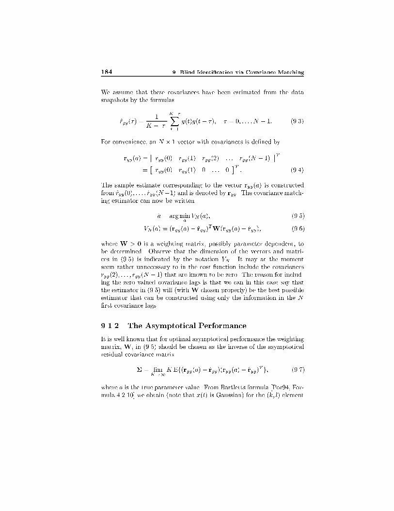
184 9 Blind Identi�cation via Covariance Matching
We assume that these covariances have been estimated from the data
snapshots by the formulas
ryy(�) =1
K � j� jK��Xt=1
y(t)y(t� �); � = 0; : : : ; N � 1: (9.3)
For convenience, an N � 1 vector with covariances is de�ned by
ryy(a) =�ryy(0) ryy(1) ryy(2) : : : ryy(N � 1)
�T=�ryy(0) ryy(1) 0 : : : 0
�T: (9.4)
The sample estimate corresponding to the vector ryy(a) is constructed
from ryy(0); : : : ; ryy(N�1) and is denoted by ryy. The covariance match-ing estimator can now be written
a = argmina
VN (a); (9.5)
VN (a) = (ryy(a)� ryy)TW(ryy(a)� ryy); (9.6)
where W > 0 is a weighting matrix, possibly parameter dependent, to
be determined. Observe that the dimension of the vectors and matri-
ces in (9.5) is indicated by the notation VN . It may at the moment
seem rather unnecessary to in the cost function include the covariances
ryy(2); : : : ; ryy(N � 1) that are known to be zero. The reason for includ-
ing the zero valued covariance lags is that we can in this case say that
the estimator in (9.5) will (withW chosen properly) be the best possible
estimator that can be constructed using only the information in the N
�rst covariance lags.
9.1.2 The Asymptotical Performance
It is well known that for optimal asymptotical performance the weighting
matrix, W, in (9.5) should be chosen as the inverse of the asymptotical
residual covariance matrix
� = limK!1
K Ef(ryy(�a)� ryy)(ryy(�a)� ryy)T g; (9.7)
where �a is the true parameter value. From Bartletts formula [Por94, For-
mula 4.2.10] we obtain (note that x(t) is Gaussian) for the (k; l) element

9.1 An Introductory Example 185
of �:
limK!1
Ef(ryy(k)� ryy(k))(ryy(l)� ryy(l))g
=
1X�=�1
ryy(�)ryy(� + k � l)
| {z }[�1]k;l
+
1X�=�1
ryy(� + k)ryy(� � l)
| {z }[�2]k;l
: (9.8)
It is easy to establish that the �rst sum in the above formula, [�1]k;l, is
a symmetric N �N Toeplitz1 matrix with the �rst row equal to�1 + 4�a2 + �a4 2�a(1 + �a2) �a2 0 : : : 0
�: (9.9)
The second matrix, �2, is a symmetric N �N Hankel2 matrix with the
�rst column equal to
�1 + 4�a2 + �a4 2�a(1 + �a2) �a2 0 : : : 0
�T: (9.10)
We have now determined the optimal weighting matrix W = ��1. It is
assumed that the indicated inverse exists. With this choice of weighting
matrix, it is shown in [Por94] that the asymptotical parameter covariance
matrix is given by
limK!1
Ef(a� �a)2g = 1
gTWg=
1
gT��1g(9.11)
where the limiting Jacobian is given by
g =@ryy(a)
@a
����a=�a
=�2�a 1 0 : : : 0
�T: (9.12)
9.1.3 A Lower Bound on the Performance
A frequently used lower bound for the estimation error covariance of
unbiased parameter estimates is the Cram�er-Rao bound (CRB). In this
scalar valued case with Gaussian processes, straight forward formulas
exist for the asymptotical CRB. If we de�ne the spectrum of y(t) by
�yy(z) = (1 + az�1)(1 + az); (9.13)
1A Toeplitz matrix is constant along the diagonals.2A Hankel matrix is constant along its anti-diagonals.

186 9 Blind Identi�cation via Covariance Matching
then the asymptotical CRB is given by a formula originally derived by
Whittle [Por94, Theorem 5.3]:
CRB�1 =1
4� i
Ijzj=1
�@ log(�yy(z))
@a
����a=�a
�21
zdz =
1
1� �a2: (9.14)
That is, we can conclude that all unbiased estimators satisfy
limK!1
K Ef(a� �a)2g � 1� �a2: (9.15)
In addition, it is possible to show [Por94] that when the number of sample
covariances, N , approaches in�nity in this model structure, the estimates
de�ned by (9.5) reach this lower bound. This is not surprising since a
Gaussian process contains all its information in the second order mo-
ments; i.e., if we use all the covariances to estimate the parameters, then
the estimator should be optimal and reach the CRB.
9.1.4 Numerical Evaluation
Now the performance of the estimator de�ned by (9.5) is evaluated and
compared with the lower bound in (9.15). The behavior of the optimally
weighted estimator in (9.5) is in Figure 9.1 evaluated as a function of
the parameter a and the number of covariance lags, N . The �gure shows
that when the number of covariance lags increases, the estimator reaches
the lower bound on the estimation error covariance.
It is important to note that two covariance lags (N = 2) are not
su�cient to reach the CRB; this is in contrast to the corresponding results
for AR-processes and is somehow surprising since we know that ryy(�) =
0 when j� j > 1. This result can be proved analytically for the investigated
MA(1) process. That is, even if the theoretical covariances are known to
be zero, the sample estimates ryy(�) for � � 2 still contain information
about the system. This is not surprising since it is known that an MA-
process has no su�cient statistic of �xed dimension when the number of
snapshots increases.
As a comparison to the optimally weighted estimator, the performance
of the estimator in (9.5) with identity weighting is shown in Figure 9.2.
Since the identity matrix is diagonal, there is with this choice of weighting
matrix no performance improvement when N is increased above 2. This
concludes the example.

9.2 Covariance Matching 187
23
45
67
8
0
0.2
0.4
0.6
0.81
2
3
4
5
6
7
8
9
Na
NormalizedCovariance
Figure 9.1: The asymptotical performance of the optimally weighted estima-
tor in (9.5) as a function of a and N . Observe that the asymptotical covariance
of the estimator is normalized with the bound in (9.15).
9.2 Covariance Matching
Covariance matching is a weighted least squares �t between the unstruc-
tured estimate of the second order statistics, Rxx(0), and a parameter-
ized thereof Rxx(0). With the statistical assumptions in Chapter 4, the
covariance matrix Rxx(0) is parameterized by the complex channel co-
e�cients in H1 (except for the �xed one) and the variances �2 and �2d.
Compared to subspace algorithms, there are thus two additional param-
eters to determine. It is convenient to collect all these parameters in a
real valued column vector
� =�hT �2 �2
d
�T; (9.16)
where h is the real valued parameter vector de�ned in (5.9). It is also
practical to work with the vectorized counterpart of the covariance ma-
trices instead of the matrices themselves. For the vectorized quantities

188 9 Blind Identi�cation via Covariance Matching
23
45
67
8
0
0.2
0.4
0.6
0.81
2
3
4
5
6
7
8
9
10
Na
NormalizedCovariance
Figure 9.2: The asymptotical performance of the estimator in (9.5) with
identity weighting and as a function of a and the number of covariance lags, N .
Observe that the asymptotical covariance of the estimator is normalized with
the bound in (9.15).
we introduce the notation
rxx(�) = vec[Rxx(0)]; (9.17)
rxx = vec[Rxx(0)]; (9.18)
where the dependence on the parameter vector is indicated in the �rst
equation. Before the cost function is introduced, some comments on the
special structure of the covariance matrix is given. First, to guarantee op-
timal performance it is necessary to separate the covariance matrix into
real and imaginary parts. We demonstrate that due to the Hermitian
structure of the covariance matrix, this separation can be achieved using
a linear transformation. Second, due to the block Toeplitz structure of
the channel matrix, the covariance matrix will also be block Toeplitz.
That is, the covariance matrix is constant along the matrix blocks on the

9.2 Covariance Matching 189
diagonals. If this block structure is not taken care of, it will make the
weighting matrix rank de�cient. First, we study the Hermitian proper-
ties.
9.2.1 Hermitian Structure
The separation into real and imaginary parts of the parameters is made in
order to simplify when taking derivatives of the cost function with respect
to the parameters. By exploiting the Hermitian structure of Rxx(0),
it is possible to obtain the corresponding separation of the vectorized
covariance matrix using a simple linear transformation. The Hermitian
structure of the covariance matrix guarantees that all diagonal entries
are real valued and all non diagonal entries appear (perhaps conjugated)
at least twice. This is the property that is used when constructing the
linear transformation. The transformation is illustrated with a simple
example.
Example 9.1. Consider the Hermitian, but otherwise arbitrary, matrix
Rxx(0) and its vectorized counterpart
Rxx(0) =
�a bc
b d
�; (9.19)
rxx(0) =�a b bc d
�T: (9.20)
From these expressions it is easily seen that the real part of b, is obtained
by the linear transformation
2Refbg = �0 1 1 0
� �a b bc d
�T: (9.21)
and the imaginary part by the linear transformation
2 i Imfbg = �0 1 �1 0
� �a b bc d
�T: (9.22)
In a similar manner it is possible to obtain the real and imaginary parts
of all other elements in a Hermitian matrix. The parameters on the
diagonal are already real and there is thus no need to separate those
parameters.
This simple example illustrates that it is straight forward to �nd a
matrix, �L, satisfying
xx =�Lrxx (9.23)

190 9 Blind Identi�cation via Covariance Matching
where xx
is a real valued column vector containing all real and imaginary
elements in the covariance matrix. Note that for Hermitian matrices,
every element appears only once in xx. The previous example is now
continued.
Example 9.2. In the previous example the selection matrix would be
�L =
2664
1 0 0 0
0 0:5 0:5 0
0 �0:5j 0:5j 0
0 0 0 1
3775 (9.24)
and the vector with real elements of the covariance matrix would look
like
xx
=�a Refbg Imfbg d
�T(9.25)
By construction, the rows of �L are orthogonal and the matrix is therefore
invertible as soon as it is square. It is easily shown by counting the
number of real elements in a Hermitian matrix that �L is always square.
Now, the transformation describing the separation of the vectorized
covariance matrix into real and imaginary parts has been described. How-
ever, our covariance matrix is not only Hermitian it is also block Toeplitz.
This property is dealt with next.
9.2.2 Block Toeplitz Structure
In addition to the Hermitian structure, the covariance matrix will in our
setup also be block Toeplitz. This introduces a small problem, the same
block element will appear on many places in the covariance matrix. If
this is not taken care of, certain weighting matrices will be rank de�cient.
We choose to handle the block Toeplitz structure in the following way.
Study the block Toeplitz matrix
A =
24 A1 A�2 A�3A2 A1 A�2A3 A2 A�1
35 : (9.26)
Knowing that A is block Toeplitz and Hermitian, A is fully speci�ed
by the �rst block column. And not only that, it is fully speci�ed by

9.2 Covariance Matching 191
the real and imaginary parts of the elements on and below the main
diagonal in the �rst column. When �tting the parameterized covariance
matrix with the unstructured estimate, it is thus only necessary to study
the parameters indicated in Figure 9.3. These parameters can easily
In this area each complex valued ele-
ment appears only once.
A =
Figure 9.3: The �gure illustrates the combined block Toeplitz and Hermitian
structure of the covariance matrix. In the indicated area each complex valued
element appears only once.
be separated into real and imaginary parts by the linear transformation
utilizing the Hermitian structure. The matrix �L in the previous section is
modi�ed in order to also take into account the block Toeplitz structure.
The new selection matrix, L, is obtained from �L by the deletion of rows
corresponding to elements that are not in the indicated area in Figure 9.3.
Summarizing, we have a selection matrix, L, that separates the vectorized
covariance matrix into real and imaginary parts and where the resulting
vector only contains each element once. This is written mathematically
xx(�) = Lrxx(�) (9.27)
xx = Lrxx (9.28)
Note that all information present in rxx is also present in xx. The only
di�erence between rxx and xx
is the separation into real and imaginary
parts and the deletion of multiple copies of (in a statistical sense) the same
element. There is thus no loss of information in this transformation. This
procedure assures optimal performance as well as it facilitates invertible
weighting matrices. Furthermore, when both the signals and the noise
are Gaussian, it is straight forward to derive the second order statistics

192 9 Blind Identi�cation via Covariance Matching
of Rxx. It is therefore easy to calculate the second order statistics of xx
as well.
9.2.3 Least Squares Estimation
After this long introduction, the covariance matching cost function is now
presented. Using the above notation, the least squares �t between the es-
timated covariance and the parameterized version can now be formulated
according to
� = argmin�
vec [ xx(�)� xx]T W vec [ xx(�)� xx] ; (9.29)
where W is a real valued symmetric positive de�nite weighting matrix
to be determined. The real valued vectors xx(�) and xx are de�ned
by (9.27) and (9.28), respectively. It remains to determine the optimal
weighting matrix W in the above criterion. The minimization of (9.29)
is a non trivial problem. Especially when the identi�ability conditions of
the system are almost violated, the numerical condition of the problem
is poor. The noise variance and the scaling factor (�2; �2d) parameterize
xx linearly, but the channel coe�cients enters bilinearly. In addition, the
number of parameters to determine is large which complicates the mini-
mization even more. In this chapter, a standard minimization approach
is used (a variant of the steepest descent). However, for future practical
use it is necessary to develop a more e�cient minimization procedure.
The next section contains an expression of the optimal weighting ma-
trix and formulas for the large sample behavior of the covariance matching
approach.
9.3 Statistical Analysis
Here, the optimal weighting matrix and large sample performance of the
estimator given by (9.29) is determined. This section is similar to the
corresponding section in Chapter 6. First, the residual covariance matrix
is determined and then the large sample behavior of the estimator is
established.
9.3.1 The Residual Covariance Matrix
It is well known that to determine the optimal weighting matrix for this
class of estimators, the residual covariance matrix is central. This covari-
ance matrix is given by

9.3 Statistical Analysis 193
Theorem 9.1. Assume that the data and noise processes both are com-plex circular and Gaussian distributed. In addition, assume that the sec-ond order statistics of these processes are given by the theoretical frame-work in Chapter 4. Then the following holds
� = K Ef( xx(�)� xx)( xx(�)� xx)T g
=
N+MX�=�(N+M)
(1� j� jK
)L (Rc
xx(�) Rxx(�))L�:
In the large sample case the expression simpli�es to
limK!1
� =
N+MX�=�(N+M)
L (Rc
xx(�) Rxx(�))L
�:
Proof. See Appendix C.5.
Now, if the inverse of the residual covariance matrix exists, we know
how to weight the criterion function optimally. This invertibility of the
residual covariance matrix is still an open question. In the numerical
evaluation of this matrix, it has always been full rank. To verify this full
rank assumption theoretically is thus a problem which needs further in-
vestigation. However, note that if �L instead of L is used in the estimator,
then the covariance matrix is rank de�cient. As in the weighted subspace
case, the optimal weighting matrix, ��1 is dependent on the true pa-
rameters. Therefore the same two step procedure is suggested for this
weighted cost function. Alternatively, it is possible to estimate Rxx(�)
directly from data using the sample covariance matrix. Both methods are
equivalent asymptotically, but for small sample sizes the behavior may
di�er.
9.3.2 The Large Sample Behavior
Now, when the residual covariance matrix is known, the determination
of the large sample properties of the estimator is straight forward. It is
only to make a Taylor series expansion of the cost function and the large
sample behavior is obtained. This is a standard procedure found in many
text books in statistical signal processing, e.g., [SS89, Por94, Lju87]. The
result of this series expansion is:

194 9 Blind Identi�cation via Covariance Matching
Theorem 9.2. Assume that the estimate of the parameter vector � is ob-tained using (9.29), possibly using a weighted approach with a consistentestimate of the weighting matrix. Then the parameters are asymptoticallyGaussian distributed with the asymptotical covariance matrix given by
limK!1
K Ef(� � �)(� � �)T g=(GWGT )�1GW�WGT (GWGT )�1:
If an optimal weighting matrix is used, then the expression simpli�es to
limK!1
K Ef(� � �)(� � �)T g = (GWGT )�1: (9.30)
In these expressions, G is the derivative of xx(�) with respect to � and
it is given by
G =
26664
�T
h (�2dH�
N INL) + ~�
T
h (INL �2dHT
N)
i�T
h(�2
dH�
N INL)� i ~�
T
h(INL �2
dHT
N)
vecT (INL)
vecT (HNH�
N)
37775LT : (9.31)
The selection matrices �h and ~�h are de�ned in (5.7) and (5.8), respec-tively.
Proof. For a proof of the parameter covariance formula, see [SS89]. Thecomputation of the derivative matrixG is straight forward and the deriva-
tion of this matrix is therefore omitted.
Note that the whiteness assumption on the signal process d(t) is ex-
ploited in the covariance matching estimator. This is in contrast to the
subspace based estimator where the covariance matrix, Rdd(0), of the
symbol vector is assumed to be arbitrary. To incorporate the diago-
nal structure of Rdd(0) in the subspace based estimator is not straight
forward. Hence, since the covariance matching exploits additional infor-
mation compared to the subspace based estimator, it can possibly out-
perform the subspace based estimator. When estimating the directions of
arrival to uncorrelated signals, it is feasible to incorporate this structure
also using the subspace based estimator [JGO].
The remaining part of this chapter contains an evaluation of these
expressions both theoretically and by simulation examples.

9.4 Numerical Comparison 195
9.4 Numerical Comparison
In this section we compare the theoretical covariance of the subspace
and covariance matching estimators. The covariance matching estimator
represents a lower attainable bound for the asymptotical covariance of all
blind estimators using only a �xed number of covariance estimates. In
0 0.1 0.2 0.3 0.4 0.5 0.6 0.7 0.8 0.9 10
1
2
3
4
5
6
Time discrete frequency
MagnitudeoftheFouriertransform
Figure 9.4: The frequency responses of the two complex valued channels in
(9.32). These channels represent an ill conditioned identi�cation scenario.
the comparison, the following two channels are investigated
H11 =
�1 + i �1:618� 1:618 i 1 + i
1 + i �1:9021� 1:9021 i 1 + i
�; (9.32)
H21 =
�1 + i 1 + i 1 + i
1 + i �1:9021� 1:9021 i 1 + i
�: (9.33)
The �rst channel, H11, represents an ill conditioned identi�cation prob-
lem while H21 represents a more well behaved channel. The frequency
responses for these two channels are plotted in Figure 9.4 and in Fig-
ure 9.5. A design parameter to be chosen for both methods is the width
of the temporal window, N . In the �rst comparison, N is chosen to 3.

196 9 Blind Identi�cation via Covariance Matching
0 0.1 0.2 0.3 0.4 0.5 0.6 0.7 0.8 0.9 10
1
2
3
4
5
6
Time discrete frequency
MagnitudeoftheFouriertransform
Figure 9.5: The frequency responses of the two complex valued channels in
(9.33). These channels represent a well behaved identi�cation scenario.
This is motivated by the fact that for larger time lags than three, the out-
puts, x1(t), from the channels are uncorrelated. Then the same results
are studied when N is increased to 4.
9.4.1 Temporal Window Length N = 3
The signal to noise ratio on the channel and the covariance of the esti-
mates are in the numerical comparisons and in the simulations de�ned
as in Chapter 4. Note that the covariance of the two variance estimates
�2 and �2dare not considered in this covariance measure. In Figure 9.6
the asymptotical covariance of the estimates of H11 are shown. The �gure
shows that the unweighted covariance matching estimates, represented
by the dashed-dotted line, are suboptimal for high signal to noise ra-
tios. The weighted covariance matching estimates , represented with a
dashed line in the �gure, are signi�cantly better for high signal to noise
ratios. For low signal to noise ratios, the di�erence between the weighted
and unweighted approaches is negligible. The weighted subspace method

9.4 Numerical Comparison 197
performs well for su�ciently large signal to noise ratios. This is also ex-
pected due to the fact that the subspace method is error free when the
noise is zero. However, the covariance matching estimator is theoretically
signi�cantly better for low signal to noise ratios.
0 10 20 30 40 50 60−70
−60
−50
−40
−30
−20
−10
0
10
20
30
Covariance matching, W = I.
Covariance matching, W = ��1.
Optimally weighted subspace.
Signal to noise ratio, SNR [dB]
Estimationerrorcovariance,MSE[dB]
Figure 9.6: A plot of the theoretical estimation error covariance for the chan-
nel coe�cients in H1
1. Both the unweighted and weighted covariance matching
estimates are displayed in the plot. For comparison, the estimation error co-
variance for the optimally weighted subspace method is also included. The
temporal window length, N , is three for all the methods in the graph. The
asymptotic performance is normalized to correspond to K = 1000 snapshots.
Figure 9.7 shows the results for the more well behaved channelH21. In
this case the covariance matching and subspace methods perform almost
equally well for reasonable signal to noise ratios. Except for a displace-
ment in the signal to noise ratio, the behavior for this channel is similar
to the ill conditioned H11.

198 9 Blind Identi�cation via Covariance Matching
0 10 20 30 40 50 60−80
−70
−60
−50
−40
−30
−20
−10
Covariance matching, W = I.
Covariance matching, W = ��1.
Optimally weighted subspace.
Signal to noise ratio, SNR [dB]
Estimationerrorcovariance,MSE[dB]
Figure 9.7: A plot of the theoretical estimation error covariance for the chan-
nel coe�cients in H2
1. Both the unweighted and weighted covariance matching
estimates are displayed in the plot. For comparison, the estimation error co-
variance for the optimally weighted subspace method is also included. The
temporal window length, N , is three for all the methods in the graph. The
asymptotic covariance is normalized to correspond to K = 1000 snapshots.
9.4.2 Temporal Window Length N = 4
It is known from investigations of the subspace method that the large
sample behavior of the estimates is improved when the temporal window
length is increased. The same behavior is perhaps not expected by the
covariance matching estimator. For covariance matching it is perhaps
reasonable to believe that the performance will improve with increasing
window lengths as long as the temporal window is smaller than M + 1,
the length of the channel. For larger time lags, x1(t) are temporally un-
correlated and it seems like no more information is added when increasing
the window length above this bound. However, the numerical (as well
as the simulation) comparisons show that this is not the case. Indeed,
also the covariance matching estimator improves the performance when

9.4 Numerical Comparison 199
N is increased over M + 1. At the end of this section a motivation for
this phenomenon is given. Now, study the plots of the numerical com-
parison when N = 4. The di�erence between Figure 9.8 and Figure 9.6
0 10 20 30 40 50 60−70
−60
−50
−40
−30
−20
−10
0
10
Covariance matching, W = I.
Covariance matching, W = ��1.
Optimally weighted subspace.
Signal to noise ratio, SNR [dB]
Estimationerrorcovariance,MSE[dB]
Figure 9.8: A plot of the theoretical estimation error covariance for the chan-
nel coe�cients in H1
1. Both the unweighted and weighted covariance matching
estimates are displayed in the plot. For comparison, the estimation error co-
variance for the optimally weighted subspace method is also included. The
temporal window length, N , is four for all methods in the graph. The asymp-
totic performance is normalized to correspond to K = 1000 snapshots.
is perhaps not that obvious. The di�erence between di�erent sizes of
the temporal window is probably better seen in Figure 9.9 where the
optimally weighted case is shown for both window lengths 3 to 9. simul-
taneously. The performance improvement when increasing the temporal
window length above N = M + 1 is negligible for most channels, but in
ill conditioned cases the di�erence is larger.
That there still exists a di�erence can be explained by the following.
Although the underlying communication system is still the same when
the window length is increased, the model of the system is changed.

200 9 Blind Identi�cation via Covariance Matching
0 10 20 30 40 50 60−80
−70
−60
−50
−40
−30
−20
−10
0
32 33 34 35 36 37 38 39−50
−49
−48
−47
−46
−45
−44
−43
−42
−41
Signal to noise ratio, SNR [dB]
Estimationerrorcovariance,MSE[dB]
Figure 9.9: The estimation error covariance for H1
1 when the optimally
weighted covariance matching estimator is used. The investigated lengths of
the temporal window are N = 3 to N = 9. The uppermost solid line corre-
sponds to N = 3 and the other window lengths follow in increasing order with
decreasing covariance. The asymptotic covariance is normalized to correspond
to K = 1000 snapshots.
For larger time lags, more and more of the temporal properties of the
underlying system are incorporated into the model. Even the fact that
the covariance matrix lag is zero for large enough time lags constitutes
information. This was also observed in the example in the beginning of
this chapter.
9.5 Simulation Examples
To investigate the �nite sample behavior, the asymptotical results are in
this section compared to simulations. The formulas for the large sample
behavior of subspace estimates have been compared to simulation results
in Chapter 6 and are therefore omitted.
In the �rst simulation H21 is estimated and the number of symbols,
K, used for the computation of the sample covariance matrix is equal to
1000. The unweighted and weighted estimates are denoted with \x" and
\*", respectively. The speed up the simulations, the weighting matrix

9.5 Simulation Examples 201
is computed using the true parameters. In Figure 9.10 the experimental
estimation errors for H21 are shown. The results are the average of 500
simulation runs. The asymptotical expressions agree very well with the
0 5 10 15 20 25−45
−40
−35
−30
−25
−20
−15
W = I
W = ��1
W = I
W = ��1
Signal to noise ratio, SNR [dB]
Estimationerrorcovariance,MSE[dB]
Figure 9.10: Simulation results for the identity weighted and optimally
weighted covariance matching estimator for the channel H2
1. The temporal
window length is equal to N = 3 and the number of snapshots in each burst is
K = 1000. The solid lines represent the theoretical covariance expressions.
simulation results for this number of snapshots.
The more ill conditioned channel, H11, shows a similar behavior, but
in this case more snapshots are needed for the asymptotical bounds to be
valid. However, even if the performance bounds do not agree perfectly
with the simulation results for �nite K, weighting does still improve the
channel estimates. This can be seen in Figure 9.11. In this case each
burst contains as much as 4000 symbols and the presented results is the
average of 400 simulation runs.
The numerical minimization of the covariance matching estimator is
very complicated in the general case. When working with ill conditioned
channels, this minimization is even more di�cult to solve. The numeri-

202 9 Blind Identi�cation via Covariance Matching
0 5 10 15 20 25−45
−40
−35
−30
−25
−20
−15
−10
−5
Signal to noise ratio, SNR [dB]
Estimationerrorcovariance,MSE[dB]
Figure 9.11: Simulation results for the identity weighted and optimally
weighted covariance matching estimator for the channel H1
1. The temporal
window length is equal to N = 3 and the number of snapshots in each burst is
K = 4000. The solid lines represent the theoretical covariance expressions.
cal minimization needs an initial channel estimate to work properly. The
simulations have shown that when the channel is ill conditioned, this ini-
tial estimate must be of very high accuracy if convergence to the optimal
parameters is to be guaranteed. To simplify the simulations and minimize
the time for the search, the minimization is in the simulations initialized
with the true channel estimates. But even in this case, divergence can
occur in some cases. In a real scenario some other algorithm is needed
for the initialization.
9.6 Conclusions
The performance of the well known subspace based estimator has been
compared to a covariance matching approach. The covariance matching

9.6 Conclusions 203
estimator achieves the lower attainable bound for the estimation error
covariance using only a pre-speci�ed subset of the second order statistics
for the case when the data symbols are assumed to be Gaussian dis-
tributed. The question whether there exists a �nite dimensional subset
of the second order statistics which yields optimal performance is still
open.
The results indicate that the di�erence between the two methods is
small for reasonable signal to noise ratios. For small signal to noise
ratios the covariance matching estimator behaves better according to the
theoretical expressions. For high signal to noise ratios the estimators
behave the same. For these small signal to noise ratios the number of
samples necessary to obtain reasonably good estimates of the channel
parameters is large. In practice, only a �nite number of input data is
available and the performance improvement for small signal to noise ratios
is therefore most of theoretical interest.
The di�erence between the two methods may be larger when applied
to real data sets. The subspace method is sensitive to errors in the detec-
tion of the dimensions of the signal and noise subspaces. The covariance
matching estimator uses the additional information that the data sym-
bols are uncorrelated and may therefore be more stable as long as this
assumption is valid.
It should be noted that the numerical minimization of the covari-
ance matching estimator is complicated and computationally intense. It
is therefore necessary to develop methods for minimization of the cost
function that are less complex.


Appendix A
Proofs and Derivations:
Direction Estimation
A.1 Derivative Expression
In this appendix, a proof of the derivative expression in (2.20) is given.
By the de�nition of ~A and b, it is clear that b spans the null space of~A�. Hence,
P?~A = Pb; (A.1)
where Pb = b(b�b)�1b� and P?~A = I � ~A( ~A� ~A)�1 ~A�. Now, take the
derivative with respect to �k,
@P?~A@�k
=@Pb
@�k: (A.2)
The derivative of a projection matrix with respect to a parameter is well
known [VO91] and the above derivatives can be expressed according to
�P?~A@ ~A
@�k~Ay � (P?~A
@ ~A
@�k~Ay)� = P?b
@b
@�kby + (P?b
@b
@�kby)�: (A.3)
Multiplying (A.3) from the right with b gives
P?b@b
@�k= �
�~Ay�� @ ~A�
@�kb; (A.4)

206 A Proofs and Derivations: Direction Estimation
where we have used the relations P?~Ab = b and ~Ayb = 0. It remains to
show that Pb@b@�k
= 0. Since b�b = c, we have
@b�
@�kb+ b�
@b
@�k= 0: (A.5)
By exploiting the complex conjugate symmetry constraint, we obtain
@b�
@�kb =
@�T
@�k���� = �T
@�
@�k= �T���
@�
@�k= b�
@b
@�k; (A.6)
which when substituted in (A.5) yields
b�@b
@�k= 0; (A.7)
b (b�b)�1b�
@b
@�k= 0; (A.8)
Pb@b
@�k= 0: (A.9)
Finally, combining (A.9) and (A.4) yields
P?b@b
@�k=
@b
@�k= �
�~Ay�� @ ~A�
@�kb; (A.10)
which completes the proof.
A.2 Analysis of the MIQML Noise Power
Estimate
Rewrite the expression for the noise power estimate in the following way
c(m� d)� = Trn�BB� � �B �B�
�Ro+Tr
n�B �B�R
o: (A.11)
By the assumptions made in the lemma, all estimated quantities in the
above equation are root-N consistent. The �rst term, BB� � �B �B�, is
thus Op(1=pN), where Op(�) denotes the probability version of the cor-
responding deterministic quantity. Using the same notation, the esti-
mated covariance matrix is related to the true covariance matrix with

A.2 Analysis of the MIQML Noise Power Estimate 207
R = R+Op(1=pN). It is thus possible to replace R with R in the �rst
term without changing the large sample behavior:
c(m� d)� = Trn�BB� � �B �B�
�Ro+Tr
n�B �B�R
o+Op(1=N)
= Trn�BB� � �B �B�
�ASA�
o+Tr
n�B �B�R
o+Op(1=N)
= TrnBB�ASA�
o+Tr
n�B �B�R
o+Op(1=N): (A.12)
The second equality above is obtained by using the identity Trf �B�B�g =TrfBB�g and the third equality is obtained by exploiting the orthogo-
nality of A and �B. If it is noted that B�A = Op(1=pN), then it is seen
that the �rst term in (A.12) is Op(1=N) which results in
c(m� d)� =Trn�B �B�R
o+Op(1=N): (A.13)
The approximation in (A.13) is used later when the direction estimates
are considered. To proceed, the following two formulas1 are needed
Trf �B �B�Rg = vec�[ �B �B�] vec[R]; (A.14)
Efvec[R�R] vec�[R�R]g = 1
N(RT R): (A.15)
Here, denotes the Kronecker product and vec[�] the vectorization op-
erator [Gra81]. Applying (A.14) to (A.13), the estimation error becomes
c(m� d)(� � ��) = vec�[ �B �B�] vec[R�R] +Op(1=N): (A.16)
From (A.16) is is noted that, since R is asymptotically Gaussian accord-
ing to the central limit theorem, the noise power is also asymptotically
Gaussian. Using (A.15) the proof is concluded with
c2(m� d)2 limN!1
N Ef(� � ��)2g
= limN!1
N vec�[ �B �B�] Efvec[R�R] vec�[R�R]g vec[ �B �B�]
= vec�[ �B �B�](RT R) vec[ �B �B�]
= vec�[ �B �B�] vec[R �B �B�R]
= ��2 Trf( �B �B�)2g: (A.17)
1For matrices A;B and C of compatible dimensions, it holds that
vec[ABC] = (CT A) vec[B] and vec�[A�] vec[B] = TrfABg.

208 A Proofs and Derivations: Direction Estimation
A.3 Analysis of the MIQML Direction Es-
timates
The �rst part of the theorem is a well known result so what remains is to
obtain expressions for Q and H. The expression for Q is obtained in a
similar way as when studying the large sample behavior of the noise power
estimate. That is, it is �rst shown that when calculating Q, nothing
changes if W1 and W2 are replaced with consistent estimates. Then Q
is computed using the statistical properties of R. The derivative of the
cost function in (2.38) with respect to �k is given by
V 0k(�) = Tr
nDk(�)
�R�TrfW2RgI
�o; (A.18)
where
Dk(�) = B0k(�)W1B
�(�) +�B0k(�)W1B
�(�)��
: (A.19)
Replacing the estimate of the noise power in (A.18) with the approxima-
tive expression in (A.13) yields
V 0k(�) = Tr
nDk(�)
�R�TrfW2RgI+Op(1=N)
�o: (A.20)
Observe that the large sample properties are unchanged if the applied
approximations leave all terms tending to zero as Op(1=pN) unchanged.
Studying (A.20) it is thus concluded that when replacing W2 with W2,
the large sample performance is unchanged. Now, note that when evalu-
ated at ��
B�(�)�R�TrfW2RgI+Op(1=N)
�= Op(1=
pN): (A.21)
This shows that
W1B�(��)
�R�TrfW2RgI+Op(1=N)
�=W1B
�(��)�R� TrfW2RgI
�+Op(1=N); (A.22)
which results in
V 0k(��) = Tr
nDk(��)
�R�Tr
nW2R
oI�o
+Op(1=N): (A.23)

A.4 A Formula for ��1s 209
Next, rewrite the derivative using the Kronecker formulas introduced in
Appendix A.2
V 0k(��) = vec�[D�
k(��)] vec[R�TrfW2RgI] +Op(1=N)
= vec�[D�k(��)]
� (Im2 � vec[Im] vec�[W�
2]) vec[R] +Op(1=N): (A.24)
Because the estimates are consistent, replacing R with R makes the �rst
term zero and the expression can be rewritten in a more useful form
V 0k(��) =vec�[D�k(
��)]
� (Im2 � vec[Im] vec�[W�
2 ]) vec[R�R] +Op(1=N): (A.25)
This expression together with (A.15) gives the (k; l) element of Q. The
transformation back to a formulation with Tr(�) is straightforward and
therefore omitted. Now, the derivation of the limiting Hessian matrix
remains. Consider the �rst derivative of the cost function
V 0k(�) = Tr
n�B0k(�)W1B
�(�) +�B0k(�)W1B
�(�)���
��R�Tr
nW2R
oI�o
= 2RenTrnB0k(�)W1B
�(�)�R� Tr
nW2R
oI�oo
: (A.26)
The second derivative is
V 00kl(�) = 2Re
�Tr
��B0kl(�)W1B
�(�) +B0k(�)W1(B
0
l(�))�
�
��R�TrfW2RgI
���: (A.27)
Evaluating this expression at � = �� and letting N ! 1 results in the
expression for H in Theorem 2.2.
A.4 A Formula for ��1s
Observe that the formula for ��1s
derived in this appendix is valid also
in the case when the signals are coherent, i.e., when rankfSg = d0 < d.
Start with
�sE�
sA = E�sRA = E�sA(A�A)�1A�RA: (A.28)

210 A Proofs and Derivations: Direction Estimation
Here, the relation spanfEsg � spanfPAg have been used. Noting that
A�RA is invertible, we obtain
�sE�
sA(A�RA)�1 = E�sA(A
�A)�1: (A.29)
Now, multiply (A.29) with A�Es to yield
�sE�
sA(A�RA)�1A�Es = E�sA(A
�A)�1A�Es = E�sEs = I
)��1s
= E�sA(A�RA)�1A�E
s: (A.30)

Appendix B
Proofs and Derivations:
Frequency Estimation
B.1 A Proof of Lemma 3.1
For notational convenience, some local de�nitions are made in this ap-
pendix. First, it turns out that it is bene�cial to study the case with
(almost) double the size of the temporal window compared to (3.8). The
notations for this size of the temporal window are:
~y(t+m) =�y(t+ 1) y(t+ 2) : : : y(t+ 2m� 1)
�T~n(t+m) =
�n(t+ 1) n(t+ 2) : : : n(t+ 2m� 1)
�T~s(t+m) =
�s(t+ 1) s(t+ 2) : : : s(t+ 2m� 1)
�T:
These de�nitions result in
~y(t) = ~s(t) + ~n(t)
= ~A(!)x(t) + ~n(t); t = m; : : : ; N �m+ 1; (B.1)

212 B Proofs and Derivations: Frequency Estimation
where x(t) is de�ned in (3.7) and the signal matrix ~A is de�ned in (3.29).
In connection with this system it is also convenient to de�ne
rs(l � k) = Efs(l)sc(k)g (B.2)
R~s = Ef~s(k)~s�(k)g = ~AS ~A�
(B.3)
R~n(�) = Ef~n(k)~n�(k � �)g: (B.4)
Note that the above de�ned noise covariance equals
R~n(�) = �
�0(2m�1��)�� I2m�1��
0��� 0��(2m�1��)
�; � � 0; (B.5)
R~n(�) = RT
~n (��); � < 0: (B.6)
The reason for introducing the double sized system is that it is assumed
in this appendix that the vector with covariance lags, r, is estimated
according to
r =1
~N
N�m+1Xt=m
~y(t)y�(t) (B.7)
where ~N = N �2m+2. Recall that when considering large sample prop-
erties (N � m) of the estimator, this special estimate of the covariance
lags is not a restriction. Finally, the second order moments of the residual
in the lemma can now be written (below, the sumP
k;lshould be read

B.1 A Proof of Lemma 3.1 213
asP
N�m+1k=m
PN�m+1l=m )
EfG�2m�1rr�G2m�1g
= Ef 1
~N2
Xk;l
G�2m�1~y(k)y�(k)y(l)~y�(l)G2m�1g
= Ef 1
~N2
Xk;l
G�2m�1~n(k)[s(l) + n(l)]
� [s�(k) + n�(k)]~n�(l)G2m�1g
=1
~N2
Xk;l
G�2m�1�Efs(l)s�(k)gEf~n(k)~n�(l)g
+Efn(l)n�(k)~n(k)~n�(l)g�G2m�1
=1
~N2
Xk;l
G�2m�1�rs(l � k)R~n(k � l)
+ E[n(l)n�(k)] E[~n(k)~n�(l)]
+ E[~n(k)n�(k)] E[n(l)~n�(l)]�G2m�1
=1
~N2
Xk;l
G�2m�1�rs(l � k)R~n(k � l)
+ �2�(l � k)I+ eme�
m
�G2m�1
=1
~N
Xk
(1� jkj~N)G�2m�1rs(�k)R~n(k)G2m�1
+1
~N�2G�2m�1G2m�1 +G2m�1eme
�
mG2m�1: (B.8)
The �rst equality stems from the fact that G�2m�1~A = 0. The third
equality follows since the signal phases are independent of the noise and
since the third order moments of Gaussian variables are zero. In the
fourth equality use is made of the formula for fourth order moments of
Gaussian random variables [JS88]. In (B.8) the sum in the last line is
rewritten using the noise covariance structure in (B.5):
1
~N
Xk
(1� jkj~N)G�2m�1rs(�k)R~n(k)G2m�1
=�
~NG�2m�1(� �R~s)G2m�1 (B.9)

214 B Proofs and Derivations: Frequency Estimation
where � is the Hadamard product and the Toeplitz matrix � is given by
� =1
~N
266664
~N ~N � 1 : : : ~N � 2m+ 2
~N � 1. . .
......
. . . ~N � 1~N � 2m+ 2 : : : ~N � 1 ~N
377775 : (B.10)
In the expression for the second order moments of the residuals in (B.8),
the last term emanates from the mean value of the residuals. This remark
results in the covariance expression for the residuals
EfG�2m�1(r� r)(r � r)�G2m�1g=
�
~NG�2m�1(��R~s + �I)G2m�1: (B.11)
Given that the covariance lags are estimated according to (B.7) the above
expression involves no large sample approximations. Also, note that the
above expression is full rank even in the �nite sample case. Finally, when
N !1 then ��R~s ! R~s which yields
limN!1
N EfG�2m�1(r� r)(r � r)�G2m�1g= �2G�2m�1G2m�1: (B.12)
This concludes the proof.
B.2 A Proof of Theorem 3.2
For convenience, the notation zl = ei!l is used in this proof. In addition,
let A be de�ned similarly to :
A = (Im�d A�m(!))Q: (B.13)
Because Us spans the same space as Am(!) and because of the special
structure of the stacked matrices, the rank of and A is the same.
To determine the rank of A we need to know the number of linearly
independent solutions x 2 C2m�d�1 to
Ax = 0: (B.14)
We start by showing the second statement in the theorem (non-orthogonal
sinusoids, d > 1). According to the statement we need to establish that

B.2 A Proof of Theorem 3.2 215
in this case exactly one non-zero vector x satis�es this equation. Since
A is a �ltering matrix constructed from Am(!), it is possible to rewrite
(B.14) to a form where Am(!) appears more direct. To do this, de�ne
X to be the m� (m� d) Toeplitz matrix
X =
26664
xm�d xm�d�1 : : : x1xm�d+1 xm�d : : : x2
......
x2m�d�1 x2m�d�2 : : : xm
37775 : (B.15)
The convolutive structure of A can now be used to show that the so-
lutions to (B.14) are equivalently given by the solutions to
A�m(!)X = 0: (B.16)
Let Xl(zk) denote the polynomial
Xl(zk) =
m�1Xi=0
xm�d+1�l+iz�i
k; l = 1; : : : ;m� d; (B.17)
which is simply a polynomial representation of the (k; l)-th element in
(B.16). Next, note the following recursion
zmXl+1(z) = zm�1Xl(z) + zmxm�d�l � x2m�d�l (B.18)
which holds for l = 1; : : : ;m� d� 1. When evaluated at the d sinusoidal
frequencies, zk, all polynomials Xl(z) must be zero for (B.16) to hold.
This results in the system of equations
zmkx1 � xm+1 = 0
zmk x2 � xm+2 = 0
......
zmk xm�d�1 � x2m�d�1 = 0; (B.19)
which must hold for k = 1; : : : ; d. When the sinusoids are non-orthogonal
there exist at least two frequencies, say, !k and !l, such that
zmk6= zm
l: (B.20)
This certi�es that the only solution to (B.19) is the all-zero solution
x1 = x2 = : : : = xm�d�1 = 0
xm+1 = xm+2 = : : : = x2m�d�1 = 0: (B.21)

216 B Proofs and Derivations: Frequency Estimation
However, note that only the beginning, x1; : : : ; xm�d�1, and the end,
xm+1; : : : ; x2m�d�1, of the parameter vector x are included in (B.21).
The d+ 1 central elements in the vector x need not be zero. From, e.g.,
the �rst column in (B.16), we see that these central elements must satisfy
(3.15) and that they therefore are unique (up to a scaling) as long as the
frequencies are distinct. The other columns in (B.16) are cyclic shifts of
the �rst column and will thus satisfy (B.16) as well. That is, in this case
there is exactly one non-zero solution x and, thus,
rankfAg = (2m� d� 1)� 1 = 2m� d� 2: (B.22)
Note that the non-zero solution corresponds to X = Gm.
Now, the case when the columns of Am(!) are orthogonal or when
d = 1 is investigated. First, when d = 1, A is full rank and thus
of rank m � 1. The attention is now shifted to the case when d > 1.
The theorem states that in this case there should exist exactly m � d
non-zero solutions to (B.14). Here, we �rst �nd m � d such linearly
independent solutions and then show that these are the only non-zero
solutions to (B.14). Noting the special structure of A it is easy to see
that A2m�d�1(!?) satis�es
AA2m�d�1(!?) = 0: (B.23)
This relation establishes that A has (at least) an m � d dimensional
right null-space and is thus of rank m� 1 or less. Now, it is also possible
to �nd a d� d matrix B such that
BA�m(!) =
�Id � : : : � �
(B.24)
where� denotes some arbitrary possibly nonzero elements. If we multiply
A according to
(Im�d B)A (B.25)
and note the m� d leading (and shifted) Id matrices in this product, the
rank is easily seen to be at least m� 1. That is,
rankfAg = (2m� d� 1)� (m� d) = m� 1: (B.26)
B.3 A Proof of Lemma 3.2
First, the formula for � is derived and by using symmetry the expression
for �r is then easily established. Using the de�nition of the complex-

B.3 A Proof of Lemma 3.2 217
valued � we obtain (omitting the dependence of G on !)
limN!1
@ vec[U�sGm]
@!k= lim
N!1
vec[U�s
@Gm
@!k]
= vec[U�s@Gm
@!k] = vec[ ~�
�1
s U�s(R � �I)@Gm
@!k]
= (Im�d ~��1
sU�s) vec[(R � �I)
@Gm
@!k] (B.27)
Note that R � �I and the derivative of Gm satisfy the same structural
relations as R and Gm in (3.38). In order to exploit this fact let ~r denote
a vector that is equal to r except for that the variance r(0) is replaced
with r(0) � �. That is, ~r is given by
~r = ~A(!)�: (B.28)
We can now continue with
limN!1
@ vec[U�sGm]
@!k= (Im�d ~�
�1
s U�s)�r
@G�2m�1(!)
@!k~r
= @G�2m�1(!)
@!k~r =
@G�2m�1(!)
@!k~A(!)�: (B.29)
Since G�2m�1(!)~A(!) = 0, we have
@G�2m�1(!)
@!~A(!) = �G�2m�1(!)
@ ~A(!)
@!(B.30)
and we get
limN!1
@ vec[U�sGm]
@!k= �G�2m�1(!)
@ ~A(!)
@!k�: (B.31)
Using the de�nition of ~� in the lemma and noting that only the kth
column in ~A depends on !k establish the formula for �. To compute
a corresponding expression for �c the same relations as exploited in the
proof of Theorem 3.1 give
�c = (J)� (B.32)
which establishes that
�r = �L� = ��LG�2m�1(!)~�S: (B.33)
The proof of the lemma is now complete.

218 B Proofs and Derivations: Frequency Estimation
B.4 A Proof of Theorem 3.4
First, the expression for the large sample estimation error covariance
matrix of the AML estimator in [SHS94] is restated. In order to do this
some new matrices need to be de�ned. First, consider the matrix
�A(!) =
2666666664
e� i(m�1)!1 : : : e� i(m�1)!d
......
e� i!1 : : : e� i!d
ei!1 : : : ei!d
......
ei(m�1)!1 : : : ei(m�1)!d
3777777775
(B.34)
which is equal to ~A(!) but with the row consisting of purely ones re-
moved. The matrix �� is the \derivative" matrix of �A and is de�ned
by
�� =h
@�a1@!1
: : : @�ad@!d
i(B.35)
where �ak is the kth column of �A. The real and imaginary parts of the
lower half of �A can due to the complex conjugate symmetry be written
B =
2666666664
cos(!1) : : : cos(!d)...
......
cos(!1(m� 1)) : : : cos(!d(m� 1))
sin(!1) : : : sin(!d)...
......
sin(!1(m� 1)) : : : sin(!d(m� 1))
3777777775
=1
2
�J I
iJ � i I
��A , T �A: (B.36)
Since the kth column in B, denoted by bk, only depends on !k, it makes
sense to de�ne the \derivative" matrix � according to
� =h
@b1@!1
: : : @bd@!d
i= T ��: (B.37)

B.4 A Proof of Theorem 3.4 219
Finally, the large sample covariance matrix of the AML estimate can be
written [SHS94]
limN!1
N Ef(!AML � !0)(!AML � !0)T g
=�2
2S�1
����?B�
��1
S�1: (B.38)
Here, �?B = I � B(B�B)�1B� has been introduced. It now only re-
mains to show that the large sample covariance matrix for the subspace
based estimator in Theorem 3.3 is equal to the expression in (B.38). The
equivalence can unfortunately \only" be established for the case of non-
orthogonal sinusoids.
From Theorem 3.3 and Lemma 3.2 we have that the asymptotic co-
variance matrix of the optimally weighted subspace based estimator is
(���y�)�1 = (S� ~��
G2m�1��yG�2m�1
~�S)�1: (B.39)
The idea is now to show that a proper middle part of (B.39) is actually a
projection matrix. To see this, de�ne the middle part to be the Hermitian
matrix
P = G2m�1�(G�2m�1G2m�1
�)yG�2m�1: (B.40)
Using the formula for �y in Theorem 3.1, the asymptotic covariance
matrix can now be written
(���y�)�1 = �2S�1�~��
P ~���1
S�1: (B.41)
By using the de�nition of the Moore-Penrose pseudo inverse it is easy
to show that PP = P. Keeping in mind that P is also Hermitian, it
is possible to conclude that it is an orthogonal projection matrix. The
question is now if it is possible to �nd a useful expression for the space
spanfG2m�1�g that the matrix P projects onto. From Theorem 3.2
and its proof it is clear that, since the center column in G2m�1 is the
single solution to x = 0,
rankfG2m�1�g = (2m� d� 1)� 1: (B.42)
It is also clear that
spanf[ ~A em ]g ? spanfG2m�1�g (B.43)
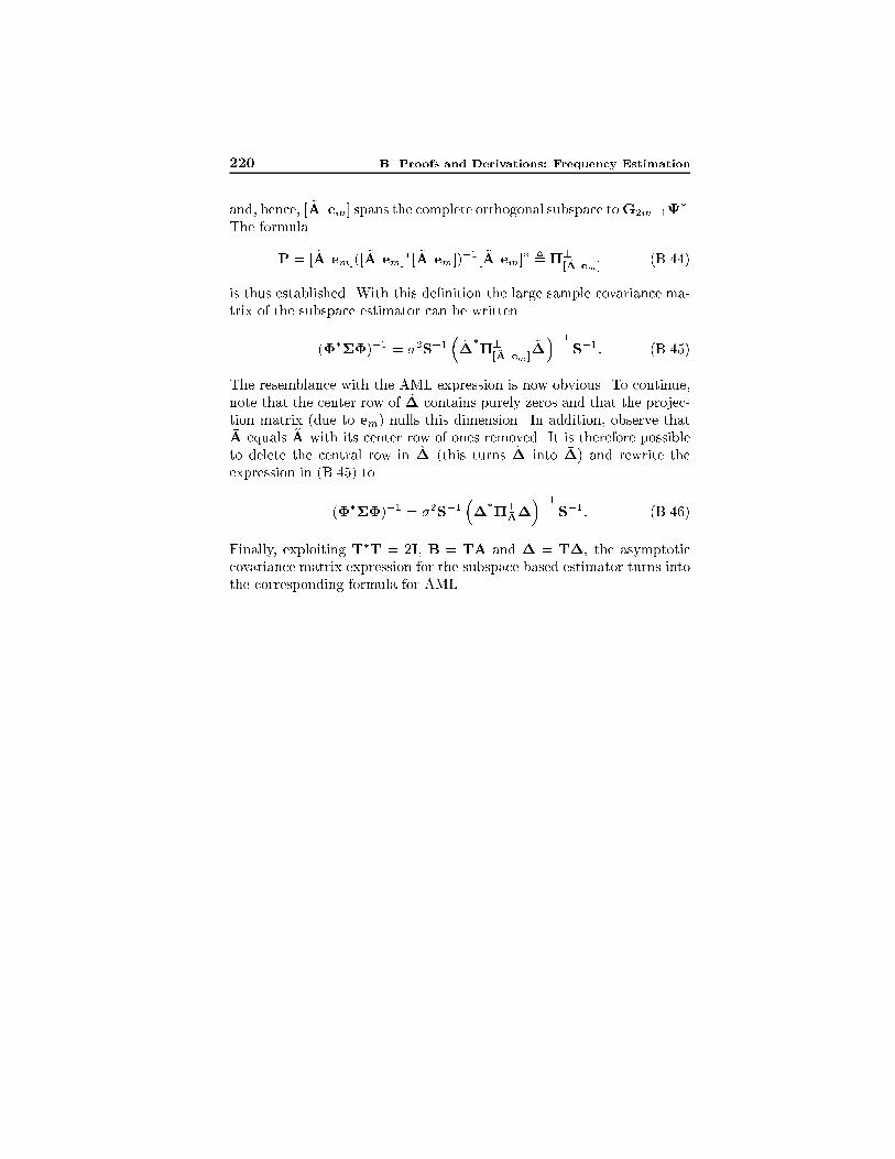
220 B Proofs and Derivations: Frequency Estimation
and, hence, [ ~A em] spans the complete orthogonal subspace toG2m�1�.
The formula
P = [ ~A em]([ ~A em]�[ ~A em])
�1[ ~A em]�,�?
[ ~A em](B.44)
is thus established. With this de�nition the large sample covariance ma-
trix of the subspace estimator can be written
(����)�1 = �2S�1�~��
�?[ ~A em]
~���1
S�1: (B.45)
The resemblance with the AML expression is now obvious. To continue,
note that the center row of ~� contains purely zeros and that the projec-
tion matrix (due to em) nulls this dimension. In addition, observe that�A equals ~A with its center row of ones removed. It is therefore possible
to delete the central row in ~� (this turns ~� into ��) and rewrite the
expression in (B.45) to
(����)�1 = �2S�1����
�?�A����1
S�1: (B.46)
Finally, exploiting T�T = 2I, B = T �A and � = T ��, the asymptotic
covariance matrix expression for the subspace based estimator turns into
the corresponding formula for AML.

Appendix C
Proofs and Derivations:
Blind Identi�cation
C.1 Mappings Between the Parameteriza-
tions
The derivation of the transformations is straight forward and shown here
only for the case when h is transformed to g. The other direction is
exactly similar and is therefore omitted. If we start with the orthogo-
nality property between HN and GN and use the vectorization formula
vec(ABC) = (CT A)vec(B) we obtain
GNHN = GNHNIN+M = 0; (C.1)
(IN+M GN )(�hhc + �h) = 0: (C.2)
After multiplication with �T
h(IN+M G�
N) and rearranging we arrive at
�T
h (IN+M G�NGN )�hhc = ��T
h (IN+M G�NGN )�h: (C.3)
The matrix on the left side in (C.3) is invertible which gives
hc = �h�T
h(IN+M G�
NGN )�h
i�1
�T
h(IN+M G�
NGN )�h: (C.4)
The covariance transformation can be obtained by calculating the deriva-
tive of (C.4) with respect to g. However, for simplicity we use a slightly

222 C Proofs and Derivations: Blind Identi�cation
di�erent approach. Denote with ~GN and ~HN small perturbations in GN
and HN obtained when estimating the parameters from noisy data,
HN = HN + ~HN ; (C.5)
GN = GN + ~GN : (C.6)
If we now use the properties GNHN = 0 and GNHN = 0 we arrive at
GNHN = (GN + ~GN )(HN + ~HN ) = GN~HN + ~GNHN = 0; (C.7)
where higher order terms are neglected. Vectorization of this last equa-
tion gives the following connection between the perturbation in the com-
plex parameters in HN (~hc) and the perturbation in the complex param-
eters in GN (~gc),
~hc = �h�T
h(IN+M G�
NGN )�h
i�1
�T
h(HT
NG�
N)�g~gc: (C.8)
Now, de�ne the complex transformation matrixTc satisfying ~hc = �Tc~gcand the real transformation matrix
T =
�RefTcg � ImfTcgImfTcg RefTcg
�: (C.9)
The connection between the covariance matrices of the real perturbations
is now easily established taking the expected value of ~hc after separation
in real and imaginary parts.
C.2 De�nition of Estimation Matrices
In this appendix expressions for and are given for both the signal
and the noise subspace parameterizations. For notational convenience,
introduce P = UnU�
n. Now proceed by,
�s = vec[PHN ] = (IN+M P)�hhc + (IN+M P)�h: (C.10)
After separation into real and imaginary parts, the following equation
holds, �Ref�sgImf�sg
�=
��rs
�is
�= sh+ s; (C.11)

C.3 The Circular Part of the Residual Covariance Matrix 223
where expressions for s and sare given by
s =
24�IN+M RefPg
��h
��IN+M ImfPg
��h�
IN+M ImfPg��h
�IN+M RefPg
��h
35 ; (C.12)
s=
24�IN+M RefPg
��h�
IN+M ImfPg��h
35 : (C.13)
For the noise subspace parameterization the process is exactly the same
and the corresponding expressions are given by
n =
24�RefUT
sg INL�N�M
��g
�� ImfUT
sg INL�N�M
��g�
ImfUTs g INL�N�M
��g
�RefUT
s g INL�N�M
��g
35 ;
(C.14)
n =
24�RefUT
sg INL�N�M
��g�
ImfUTs g INL�N�M
��g
35 : (C.15)
C.3 The Circular Part of the Residual Co-
variance Matrix
In this appendix a proof of Theorem 6.1 is given. In the �rst section,
some additional general formulas and notation regarding convergence of
stochastic variables are described. Proceeding with the proof, the key
idea is to relate large sample properties of Un and Us to properties of
the sample covariance matrix estimate, Rxx(0). This relation is derived
in the second section in this appendix. Next, the covariance matrix of the
residual vector is easily found by studying the second order properties of
Rxx(0). In the last section, the results are combined which completes
the proof.
C.3.1 Some Additional Notation
First, the well known formula for the expected value of four stochastic
Gaussian variables can [JS88] be generalized to the case of two complex
valued Gaussian distributed matrices A and D, and two complex valued

224 C Proofs and Derivations: Blind Identi�cation
Gaussian column vectors b and c. The formula is as follows,
EfAbc�Dg =EfAbgEfc�Dg+Efc� AgEfD bg+EfAEfbc�gDg� 2EfAgEfbgEfc�gEfDg: (C.16)
Second, a sequence of scalar random variables is said to be bounded in
probability [Por94] if, for all � > 0, there exists � > 0 such that,
limK!1
PfjXK j > �g < �: (C.17)
The notation XK = Op(1) indicates that XK is bounded in probabil-
ity. Now, let an be a sequence of positive real numbers. The nota-
tion XK = Op(aK) means that XK=aK = Op(1). A vector is said to be
Op(aK) if each of its components is Op(aK). The following formula is
useful when working with this \ordo" notation,
XK = Op(aK)
YK = Op(bK)
o) XKYK = Op(aKbK): (C.18)
Now we proceed with the proof of Theorem 6.1.
C.3.2 Connection to the Sample Covariance Matrix
The connection between the large sample properties of the sample covari-
ance matrix estimate, Rxx(0), and the subspace estimates Un and Un
are established in the following lemma:
Lemma C.1. Assume that the row space of GN is orthogonal to thecolumn space of Us and that HN is orthogonal to the column space ofUn; i.e., GNUs = 0 and U�nHN = 0. If, in addition, EfnN (t)n�N (t)g =�2INL, then the following two equations hold
GNUs =GNRxx(0)Us(�s � �2IN+M )�1 +Op(1=K)
UnU�
nHN =�UnU�
nRxx(0)Us(�s � �2IN+M )�1U�sHN +Op(1=K)
Proof. The proof is similar to the one in [SS91]. The second equation
in the Lemma can be established from the �rst one and therefore the
�rst statement is proved initially. In the proof the following notational
convention is used,
Us = Us + ~Us; (C.19)

C.3 The Circular Part of the Residual Covariance Matrix 225
where ~Us is Op(1=pK). The same notation applies for other estimates
in this appendix. The lemma is proved by studying the following equality
GNRxx(0)Us = GNUs�s: (C.20)
The left part of this equality can be rewritten in the following way
GNRxx(0)Us = GN (Rxx(0) + ~Rxx(0))(Us + ~Us)
= GN (Rxx(0)Us +Rxx(0) ~Us + ~Rxx(0)Us + ~Rxx(0) ~Us)
= GN (Rxx(0)Us + ~Rxx(0)Us + ~Rxx(0) ~Us)
= GN (Rxx(0)Us + Rxx(0)Us + ~Rxx(0) ~Us)
= GN
��HNRdd(0)H
�
N+ �2INL
�Us
+ Rxx(0)Us + ~Rxx(0) ~Us
�= �2GNUs +GNRxx(0)Us +GN
~Rxx(0) ~Us
= �2GNUs +GNRxx(0)Us +Op(1=K): (C.21)
Here, the equalities GNRxx(0)Us = 0 and GNHN = 0 have been used.
The right part of (C.20) can be rewritten according to,
GNUs�s =GN (Us + ~Us)(�s + ~�s)
=GN (Us�s +Us~�s + ~Us�s + ~Us
~�s)
=GN ( ~Us�s + ~Us~�s)
=GN (Us�s + ~Us~�s)
=GNUs�s +Op(1=K): (C.22)
Now, using the original equality (C.20),
�2GNUs +GNRxx(0)Us =GNUs�s +Op(1=K) (C.23)
and the �rst statement in the lemma follows. To see that the second
statement is true, introduce the notation Pn = UnU�nand Ps = U
sU�s.
Estimates of these projection matrices converge to their true values with
an error that behaves like Op(1=K). Now, study the projection of HN

226 C Proofs and Derivations: Blind Identi�cation
on to the noise subspace,
UnU�nHN = PnPnHN = Pn(Pn
+ ~Pn)HN
= Pn~PnHN = Pn
~PnHN +Op(1=K2)
= PnPnHN +Op(1=K2) = Pn(INL � Ps)HN +Op(1=K
2)
= �PnPsHN +Op(1=K2)
= �Pn(Us + ~Us)(U�
s+ ~U�
s)HN +Op(1=K
2)
= �Pn~Us(U�
s+ ~U�
s)HN +Op(1=K
2)
= �Pn~UsU
�
sHN +Op(1=K)
= �PnUsU�
sHN +Op(1=K): (C.24)
In the last expression, a matrix in the noise subspace is multiplied with
an estimate of the signal subspace. The �rst statement in the lemma has
already established the link between such an expression and the sample
covariance matrix estimate. Hence, by using the �rst statement in the
lemma, the second statement is now proved.
Next, the second order properties of Rxx(0) are determined.
C.3.3 Covariance Properties of Projected Rxx(0)
To proceed, it is only to use the properties of Rxx(0) to calculate the
residual covariance matrix for both the signal and noise subspace method.
Before using these properties, it is convenient to apply the vectorization
operator to the expression in Lemma C.1 and arrive at,
�n = vechGNUs
i=��T INL�(N+M)
�vec
hGNRxx(0)
i+Op(1=K);
(C.25)
where � = Us(�s � �2IN+M )�1 has been introduced. For the signal
subspace parameterization the corresponding expression is
�s = vechUnU�nHN
i=�HT
NUc
s�T INL
�vec
hUnU
�
nRxx(0)i+Op(1=K): (C.26)
From (C.25) and (C.26) we note that the calculation of the second order
statistics of the residual errors for both the signal and noise subspace

C.3 The Circular Part of the Residual Covariance Matrix 227
parameterizations can be cast into the same framework. We are in both
cases interested in the second order statistics of the sample covariance
matrix when it is pre-multiplied with a matrix orthogonal to the signal
subspace. An expression for this is given in the following Lemma,
Lemma C.2. Assume that the row space of GN is orthogonal to thecolumn space of HN (or equivalently the column space of Us) and thatthe covariance of the complex Gaussian noise vectors, Rnn(�), is zero if�n < j� j, then
Efvec[GNRxx(0)] vec�[GNRxx(0)]g = vec[GNRnn(0)] vec
�(GNRnn(0))
+1
K2
�nX�=��n
(K � j� j) (Rc
xx(�) GNRnn(�)G
�
N)
Proof. The proof is straight forward using the formula for the expected
value of four complex variables in [JS88]. However, it is convenient to
�rst use the the orthogonality property between GN and HN in order
to reduce the number of terms. Inserting the expression for the sample
estimate of the covariance matrix we obtain
GNRxx =1
KGN
KXt=1
xN (t)x�
N (t)
=1
KGN
KXt=1
[HNdN+M (t) + nN (t)][d�
N+M (t)H�N + n�N (t)]
=1
K
KXt=1
[GNnN (t)d�
N+M (t)H�N+GNnN (t)n
�
N(t)]: (C.27)
Note that the above equation is linear in the data symbols dN+M (t) but
quadratic in nN (t). This is why the covariance of the subspace estimates
are only dependent on the second order statistics of the data symbols
and independent on higher order statistics of the data symbols. After

228 C Proofs and Derivations: Blind Identi�cation
this simpli�cation we have
vec[GNRxx] vec�[GNRxx]
=1
K2
KXt=1
KX�=1
vec[GNnN (t)d�
N+M (t)H�N] vec�[GNnN (�)d
�
N+M (�)H�N]
+1
K2
KXt=1
KX�=1
vec[GNnN (t)d�
N+M (t)H�N] vec�[GNnN (�)n
�
N(�)]
+1
K2
KXt=1
KX�=1
vec[GNnN (t)n�
N (t)] vec�[GNnN (�)d
�
N+M (�)H�N ]
+1
K2
KXt=1
KX�=1
vec[GNnN (t)n�
N (t)] vec�[GNnN (�)n
�
N (�)]: (C.28)
Applying the expectation operator to (C.28) only the �rst and last double
sums are nonzero. This is because third order moments of Gaussian
variables are zero. The problem is thus simpli�ed to
Efvec[GNRxx(0)] vec�[GNRxx(0)]g
=E
(1
K2
KXt=1
KX�=1
vec[GNnN (t)d�
N+M (t)H�N ]
� vec�[GNnN (�)d�
N+M (�)H�N]
)
+E
(1
K2
KXt=1
KX�=1
vec[GNnN (t)n�
N(t)] vec�[GNnN (�)n
�
N(�)]
):
(C.29)
We now proceed by calculating the expected values of the terms in the
�rst double sum.
E�vec
�GNnN (t)d
�
N+M (t)H�N�vec�
�GNnN (�)d
�
N+M (�)H�N�
= E�(Hc
N GN ) vec[nN (t)d�
N+M (t)] vec�[nN (�)d�
N+M (�)](HT
N G�N )
= (Hc
N GN ) E��dcN+M (t) nN (t)
� �dTN+M (�) n�N (�)
�(HT
N G�N )= (Hc
N GN ) E��dcN+M (t)dTN+M (�)
� (nN (t)n�
N (�))(HT
N G�N )= (Hc
N GN )(Rc
dd(t� �) Rnn(t� �))(HT
N G�N )= (HRdd(t� �)H�)
c (GNRnn(t� �)G�N ) : (C.30)

C.3 The Circular Part of the Residual Covariance Matrix 229
The expected value of the terms in the second double sum is a little bit
more complicated. First, separate GN from the noise terms,
E fvec[GNnN (t)n�
N(t)] vec�[GNnN (�)n
�
N(�)]g
= (INL GN ) E fvec[nN (t)n�N (t)] vec�[nN (�)n�N (�)]g (INL G�N ):(C.31)
Now, the expected value of the noise terms is calculated using the formula
for four complex Gaussian variables [JS88],
E fvec[nN (t)n�N (t)] vec�[nN (�)n�N (�)]g= E
�(INL nN (t))ncN (t)nTN (�) (INL n�N (�))
= E fvec[nN (t)n�N (t)]gE fvec�[nN (�)n�N (�)]g+E
�nTN (�) INL nN (t)
E fINL n�N (�) ncN (t)g
+E�(INL nN (t)) E
�ncN (t)n
T
N (�)(INL n�N (�))
: (C.32)
In the above expression, one term disappears due to the assumption of
circularly symmetric distributed noise variables. The �rst expected value
in (C.32) is simply vec[Rnn(0)] vecT [Rnn(0)]. The last expected value
in (C.32) is easily calculated using the following formula for two column
vectors a and b of dimension NL � 1 and a matrix C of dimension
NL�NL
(INL a)C(INL bT ) = C (abT ): (C.33)
The last expected value in (C.32) is now calculated below using the above
formula,
E�(INL nN (t)) E
�ncN(t)nT
N(�)(INL n�N (�))
= E f(INL nN (t))Rc
nn(t� �)(INL n�N (�))g= E fRc
nn(t� �) (nN (t)n
�
N(�))g
= Rc
nn(t� �)Rnn(t� �): (C.34)
The terms in the second double sum can now be written
E fvec[GNnN (t)n�
N (t)] vec�[GNnN (�)n
�
N (�)]g= vec[GNRnn(0)] vec
�[GNRnn(0)]
+ (Rc
nn(t� �) (GNRnn(t� �)G�N ): (C.35)

230 C Proofs and Derivations: Blind Identi�cation
Using (C.35) and (C.30) the expected value in (C.29) can now be written
on the following form
Efvec[GNRxx(0)] vec�[Rxx(0)]g
=1
K2
KXt=1
KX�=1
�(HNRdd(t� �)H�
N)c (GNRnn(t� �)G�
N)
+ vec[GNRnn(0)] vec�[GNRnn(0)] +Rc
nn(t� �) (GNRnn(t� �)G�
N)�
=�4 vec[GN ] vec�[GN ] +
1
K2
KXt=1
KX�=1
Rc
xx(t� �) (GNRnn(t� �)G�
N):
(C.36)
The expression in the summation is only dependent on t � � and the
double sum can due to this be converted into a single sum. In addition,
we use the assumption that the covariance matrix is zero if the time lag
exceeds �n. This gives the �nal expression for the sum
Efvec[GNRxx(0)] vec�[GNRxx(0)]g
=vec[GNRnn(0)] vec�[GNRnn(0)]
+1
K
�nX�=��n
(1� j� jK
)�Rc
xx(�) (GNRnn(�)G
�
N):�: (C.37)
This concludes the proof of the lemma.
C.3.4 Final Results
Here, di�erent results from the previous two sections are collected in
order to complete the proof. We only complete the proof for �n because
�s is obtained exactly in the same way. Recall the formula,
�n = vec[GNUs] =��T INL�(N+M)
�vec[GN Rxx(0)] +Op(1=K):
(C.38)
In the rest of this section we use I instead of INL�(N+M). Because
Rxx(0) converges in probability and in mean square to Rxx(0) with an
error that behaves like Op(1=pK), the expression in (C.38) tends to zero
like Op(1=pK). Using this observation we obtain the following for the

C.4 The Non-Circular Part of the Residual Covariance Matrix 231
residual �n,
�n��
n
=��T I
�vec[GNRxx(0)] vec
�[GNRxx(0)] (�c I) +Op(1=K
3=2)
(C.39)
After taking the expected value and using the fact that, when Rnn(0) is
a scaled identity matrix, (�T I) vec[GNRnn(0)] = 0 the �nal result is
obtained,
limK!1
K Ef�n��ng =�nX
�=��n
��TRc
xx(�)�c)� (GNRnn(�)G
�
N ) :
(C.40)
Due to the covariance properties of the data symbols and the additive
noise, �n is equal to N � 1 in our blind identi�cation setup. Noting this
the theorem is proved.
C.4 The Non-Circular Part of the Residual
Covariance Matrix
In this appendix, a proof of Theorem 6.2 is given. The proof follows the
line suggested in Section 6.3 and is in great detail analogous to the proof
in the previous appendix. Using the connection between the covariance
estimate and the subspaces estimates established in Appendix C.3, the
large sample covariance of the non-circular part is determined.
C.4.1 The Covariance Matrix of the Non-CircularPart
The connection between the covariance matrix estimate and the subspace
estimates is given in Appendix C.3, but for ease of reference it is repeated

232 C Proofs and Derivations: Blind Identi�cation
here,
�n =vechGNUs
i=��T INL�(N+M)
�vec
hGNRxx(0)
i+Op(1=K); (C.41)
�s =vechUnU
�
nHN
i=�HT
NUc
s�T INL
�vec
hUnU
�
nRxx(0)i+Op(1=K): (C.42)
Thus, if we can calculate the expected value of
vec[GN Rxx(0)] vecT [GNRxx(0)]; (C.43)
where the row space of GN is orthogonal to Us, then the proof is almost
completed. This expected value is given in the following lemma,
Lemma C.3. Assume that GN is orthogonal to HN (or equivalentlyUs). In addition, assume that the complex Gaussian noise vectors satisfythe assumptions in Section 4.4.1. De�ne the (i; j) block of the (NL)2 �(NL)2 matrix �(t) according to
�i;j(t) = Rnn(t)ejeT
i Rc
nn(t);
where ei and ej are the ith and jth column of INL respectively. De�ne ��
and ~� according to
~� =1
K2
N�1X�=�N+1
(K � j� j)�(�) �� =
N�1X�=�N+1
�(�):
Then the following holds
Efvec[GNRxx(0)] vecT [GNRxx(0)]g = �4n vec[GN ] vec
T [GN ]
+ (INL GN )~�(INL GT
N):
Proof. The proof is straight forward using the formula for four complex
variables already used in Appendix C.3. The expected value in the the-

C.4 The Non-Circular Part of the Residual Covariance Matrix 233
orem is written on the following form,
vec[GNRxx] vecT [GNRxx]
=1
K2
KXt=1
KX�=1
vec[GNnN (t)d�
N+M (t)H�N ] vecT [GNnN (�)d
�
N+M (�)H�N ]
+1
K2
KXt=1
KX�=1
vec[GNnN (t)d�
N+M (t)H�N ] vecT [GNnN (�)n
�
N (�)]
+1
K2
KXt=1
KX�=1
vec[GNnN (t)n�
N(t)] vecT [GNnN (�)d
�
N+M (�)H�N]
+1
K2
KXt=1
KX�=1
vec[GNnN (t)n�
N(t)] vecT [GNnN (�)n
�
N(�)]: (C.44)
Applying the expectation operator to (C.44), only the last double sum is
nonzero. This is due to the fact that third order moments of Gaussian
variables are zero and that the Gaussian noise is assumed to be circularly
symmetric. Note that this holds independently of the distribution of the
data symbols. The problem is thus simpli�ed to
Efvec[GNRxx] vecT [GNRxx]g
=E
(1
K2
KXt=1
KX�=1
vec[GNnN (t)n�
N(t)] vecT [GNnN (�)n
�
N(�)]
):
(C.45)
Now, separate GN from the noise terms,
E�vec[GNnN (t)n
�
N(t)] vecT [GNnN (�)n
�
N(�)]
= (INL GN ) E
�vec[nN (t)n
�
N(t)] vecT [nN (�)n
�
N(�)]
(INL GT
N):
(C.46)
The expected value in the equation above consists of NL�NL blocks. It
can be shown that the (i; j) block of E�vec[nN (t)n
�
N(t)] vecT [nN (�)n
�
N(�)]
can be written as
�4neieT
j +Rnn(t� �)ejeT
i Rc
nn(t� �): (C.47)
Note that the �rst part can be written as the (i; j) block of
vec[INL] vecT [INL] (C.48)
From this observation the lemma follows.

234 C Proofs and Derivations: Blind Identi�cation
Combining equations (C.41) and (C.42) with the result in the lemma
now completes the proof of Theorem 6.2.
C.5 The Large Sample Properties of the Sam-
ple Covariance Matrix
In this appendix, the large sample properties of the sample covariance
matrix are derived when it is assumed that both the data symbols and
the noise are Gaussian processes. The covariance matrix, denoted � is
given by,
� = limK!1
K Efvec[Rxx(0)� Rxx(0)] vec�[Rxx(0)� Rxx(0)]g; (C.49)
whereK is the number of samples used in the estimation of the covariance
matrix, Rxx(0) is the true covariance of the received vectors and Rxx(0)
is the sample estimate of the covariance matrix. To derive a formula for
(C.49) we �rst calculate the following covariance,
~� = Efvec[Rxx(0)] vec�[Rxx(0)]g: (C.50)
When ~� is known, (C.49) is easily calculated. The calculation of ~� is
straight forward using the formula for the fourth order moment of Gaus-
sian matrices. If we substitute (1=K)P
K
t=1 xN (t)x�
N(t) for the sample

C.5 The Large Sample Properties of the Sample Covariance Matrix 235
covariance, we obtain
~� = Envec[
1
K
KXt=1
xN (t)x�
N (t)] vec�[1
K
KXt=1
xN (�)x�
N (�)]o
= Envec[
1
K
KXt=1
(HNdN (t) + nN (t))(d�
N (t)H�
N + n�N (t))] vec�[�]o
= Envec
h 1K
KXt=1
(HNdN (t)d�
N(t)H�
N+HNdN (t)n
�
N(t)
+ nN (t)d�
N(t)H�
N+ nN (t)n
�
N(t))
i
vec�h 1K
KX�=1
(HNdN (�)d�
N(�)H�
N+HNdN (�)n
�
N(�)
+ nN (�)d�
N(�)H�
N+ nN (�)n
�
N(�))
io
=1
K2
KXt=1
KX�=1
Envec[HNdN (t)d
�
N(t)H�
N] vec�[HNdN (�)d
�
N(�)H�
N]
+ vec[HNdN (t)d�
N(t)H�
N] vec�[nN (�)n
�
N(�)]
+ vec[HNdN (t)n�
N (t)] vec�[HNdN (�)n
�
N (�)]
+ vec[nN (t)d�
N(t)H�
N] vec�[nN (�)d
�
N(�)H�
N]
+ vec[nN (t)n�
N (t)] vec�[HNdN (�)d
�
N (�)H�
N ]
+ vec[nN (t)n�
N(t)] vec�[nN (�)n
�
N(�)]
o; (C.51)
where we have used the fact that the noise is a complex circular Gaussian
stochastic process with zero mean. (For example, third order moments
of the noise are zero). Note that it is not necessary to assume anything
about the distribution of the data symbols to arrive at (C.51). Though, in
the following we assume that also the data symbols are circularly complex
Gaussian distributed with zero mean. Now, calculate the �rst summation

236 C Proofs and Derivations: Blind Identi�cation
term in (C.51),
Efvec[HNdN (t)d�
N (t)H�
N ] vec�[HNdN (�)d
�
N (�)H�
N ]g= Ef(Hc
NHN) vec[dN (t)d
�
N(t)]((Hc
NHN ) vec[dN (�)d
�
N(�)])�g
= Ef(Hc
NHN) vec[dN (t)d
�
N(t)] vec�[dN (�)d
�
N(�)](HT
NH�
N)
= (Hc
NHN) Efvec[dN (t)d�N (t)] vec�[dN (�)d�N (�)]g(HT
NH�
N):
(C.52)
We see that the �rst and the last term in (C.51) can be treated simul-
taneously. To continue use the formula for the expected value of four
complex Gaussian matrices [JS88] and in addition use the identity,
(INL a)C(INL bT ) = C (abT ); (C.53)
where a and b are column vectors of dimensionNL andC is anyNL�NL
matrix. Now, expand the expectation value in (C.52) using ordinary
Kronecker formulas,
Efvec[dN (t)d�N (t)] vec�[dN (�)d�N (�)]g= Ef(INL dN (t))dcN (t)dTN (�)(INL d�N (�))g= Efvec[dN (t)d�N (t)]gEfvec[dN (�)d�N (�)]g+EfdT
N(�) INL dN (t)gEfINL d�N (�) dcN (t)g
+Ef(INL dN (t)) EfdcN (t)dTN (�)g(INL d�N (�))g= vec[Rdd(0)] vec
�[Rdd(0)] +Rc
dd(t� �)Rdd(t� �): (C.54)
This shows that the �rst and last terms in (C.51) are equal to
vec[HNRdd(0)H�
N ] vec�[HNRdd(0)H
�
N ]
+ (HNRdd(t� �)H�N)c (HNRdd(t� �)H�
N); (C.55)
vec[Rnn(0)] vec�[Rnn(0)] +Rc
nn(t� �)Rnn(t� �): (C.56)
By inspection we see that the second and �fth terms in (C.51) are equal
to
vec[HNRdd(0)H�
N] vec�[Rnn(0)] (C.57)
vec[Rnn(0)] vec�[HNRdd(0)H
�
N ]; (C.58)

C.5 The Large Sample Properties of the Sample Covariance Matrix 237
respectively. The terms left to determine are the two in the middle.
Efvec[nN (t)d�N (t)H�N ] vec�[nN (�)d�N (�)H�N ]g= Ef(Hc
N INL)(INL nN (t))dcN (t)
� [(Hc
N INL)(INL nN (�))dcN (�)]�g= Ef(Hc
N INL)(INL nN (t))dcN (t)
� dTN(�)(INL n�N (�))(HT
N INL)g
= Ef(Hc
N INL)(d
c
N(t)dT
N(�)) (nN (t)n
�
N(�))(HT
N INL)g
= Ef(Hc
Ndc
N (t)dT
N (�)HT
N ) (nN (t)n�
N (�))g= (HNRdd(t� �)H�
N)c Rnn(t� �) (C.59)
Efvec[HNdN (t)n�
N (t)] vec�[HNdN (�)n
�
N (�)]g=Ef(INL HN )(INL dN (t))ncN (t)nTN (�)(I d�N (�))(INL H�N)g=Rc
nn(t� �) (HNRdd(t� �)H�N ) (C.60)
Now, we have expressions for all the terms in the summation and it thus
only remains to sum the results up,
~� =1
K2
KXt=1
KX�=1
vec[HNRdd(0)H�
N] vec�[HNRdd(0)H
�
N]
+ (HNRdd(t� �)H�N)c (HNRdd(t� �))
+ vec[HNRdd(0)H�
N ] vec�[Rnn(0)]
+Rc
nn(t� �) (HNRdd(0)H
�
N)
+ vec[Rnn(0)] vec�[HNRdd(0)H
�
N]
+ (HNRdd(t� �)H�N )c Rnn(t� �)
+ vec[Rnn(0)] vec�[Rnn(0)]
+Rc
nn(t� �) Rnn(t� �): (C.61)

238 C Proofs and Derivations: Blind Identi�cation
The previous formula gives an explicit solution for ~�. However, a more
tractable form is obtained after some further manipulations,
~� = vec[Rxx(0)] vec�[Rxx(0)] +
1
K2
K�1X�=�(K�1)
(K � j� j)Rc
xx(�) Rxx(�)
= vec[Rxx(0)] vec�[Rxx(0)]
+1
K2
K�1X�=�(K�1)
(K � j� j)RT
xx(��)Rxx(�): (C.62)
Note that the two above formulas for ~� are exact for all values of K, no
terms are neglected. To calculate � when ~� is given is trivial and results
in the following expressions
� = limK!1
K Efvec[Rxx(0)� Rxx(0)] vec�[Rxx(0)� Rxx(0)]g
= limK!1
K�1X�=�(K�1)
(1� j� jK
)Rc
xx(�)Rxx(�) (C.63)
In Chapter 4 one assumption was that the covariance of the received data
vectors is zero if the time lag exceeds �n. Using this property the �nal
result is obtained,
� = limK!1
K Efvec[Rxx(0)� Rxx(0)] vec�[Rxx(0)� Rxx(0)]g
=
�nX�=��n
Rc
xx(�)Rxx(�) =
�nX�=��n
RT
xx(��) Rxx(�): (C.64)

Appendix D
Notation
In general, matrices are denoted by uppercase and vectors with lowercase
boldface letters, e.g., H and �. Normal typeface is used for scalar vari-
ables, e.g., N and � . Below, general matrices common in the literature
and some mathematical operations and their corresponding notations are
introduced. In many cases, the subscript on a matrix or a vector indicates
its dimension (or, alternatively, its block dimension). If the dimension is
clear from the context, the subscript is omitted. Note that, in general, t
indicates discrete time. Estimated quantities are denoted with (�). For
example, the estimate of A is A.
m� n The dimension of a matrix with m rows and n columns.
0i�j An i� j matrix with all entries equal to zero.
Im The identity matrix of dimension m�m.
Jm This matrix is commonly referred to as the exchange
matrix. It is equal to the identity matrix Im with the
column order reversed:
Jm =
266664
0 : : : 0 1... . .
.1 0
0 . ..
. .. ...
1 0 : : : 0
377775

240 D Notation
Dm An m �m matrix with ones on the diagonal below the
main diagonal and zeros elsewhere:
D =
266666664
0 : : : : : : : : : 0
1. . .
...
0 1. . .
......
. . .. . .
. . ....
0 : : : 0 1 0
377777775
diag[a1; : : : ; am] A matrix with the indicated elements on its main diag-
onal and zeros elsewhere.
AT ;A�;Ac Transpose, complex conjugate transpose and complex
conjugate of A, respectively.
TrfAg The trace of the square matrix A.
spanfAg The space spanned by the columns in A.
rankfAg The rank (number of independent rows or columns) of
the matrix A.
kAkF The Frobenius norm of the matrix A. This norm can
alternatively be written kAk2F= TrfAA�g.
Ay The Moore-Penrose pseudo inverse ofA. See, e.g., [RM71,
BIG73].
RefAg; ImfAg The real and imaginary parts of A, respectively.
vec[A] The column vector obtained by ordering the columns of
the matrix A on top of each other in a column vector.
See further [Bre78, Gra81].
[A]k;l The (k; l) element in the matrix A. Note that when A
is a block matrix, the notation may be used to indicate
the (k; l) block element.
AB The Kronecker product of the matrices A and B. See,
e.g., [Bre78, Gra81].

D Notation 241
A�B The Hadamard product of the matrices A and B. The
(i; j) element of this product is equal to [A]i;j [B]i;j . See
[SM97, Appendix A.5].
A � B For two positive semi-de�nite matrices A and B, this
states that also the di�erence A�B is positive semi-
de�nite. That is, x�(A�B)x � 0 for all complex-valued
column vectors x.
argminx
f(x) The minimizing argument of the function f(x).
Ef�g Mathematical expectation.
i i =p�1.
� Denotes multiplication when there is a speci�c need to
emphasize this operation, e.g., a line break in an equa-
tion.
bxc The largest integer less than or equal to x.
cond(A) The condition number of the matrixA. In this thesis the
condition number is de�ned as the largest singular value
ofA divided by the smallest non zero singular value ofA.
See [GvL89, page 230] for a more thorough description.


Bibliography
[AdCS98] Jaouhar Ayadi, Elisabeth de Carvalho, and Dirk T.M.
Slock. Blind and semi-blind maximum likelihood meth-
ods for FIR multichannel identi�cation. In InternationalConference on Acoustics, Speech, and Signal Processing(ICASSP), pages 3185{3188, Seattle, Washington, USA,
May 1998.
[AMCG+97] K. Abed-Meraim, J.F. Cardoso, A. Gorokhov, P. Loubaton,
and E. Moulines. On subspace methods for blind channel
identi�cation of single-input multiple-output FIR systems.
IEEE Transactions on Signal Processing, 45(1):42{55, Jan-uary 1997.
[AMVW91] S�oren Andersson, M. Millnert, Mats Viberg, and
Bo Wahlberg. An adaptive array for mobile communica-
tion systems. IEEE Transactions on Vehicular Technology,40(1):230{236, 1991.
[BG84] Albert Benveniste and Maurice Goursat. Blind equaliz-
ers. IEEE Transactions on Communications, 32(8):871{
883, August 1984.
[BIG73] Adi Ben-Israel and Thomas N.E. Greville. Generalized In-verses: Theory and Applications. John Wiley & Sons, 1973.
[BM86] Yoram Bresler and Albert Macovski. Exact maximum like-
lihood parameter estimation of superimposed exponential
signals in noise. IEEE Transactions on Acoustics, Speech,and Signal Processing, 34(5):1081{1089, October 1986.

244 Bibliography
[B�oh84] Johann F. B�ohme. Estimation of source parameters by
maximum likelihood and nonlinear regression. In Inter-national Conference on Acoustics, Speech, and Signal Pro-cessing (ICASSP), volume 1, pages 7.3.1{7.3.4, San Diego,
California, March 1984. IEEE.
[Bre78] John W. Brewer. Kronecker products and matrix calculus
in system theory. Transactions on Circuits and Systems,25(9):772{781, Sept 1978.
[BS92] Philip Balaban and Jack Salz. Optimum diversity com-
bining and equalization in digital data transmission with
applications to cellular mobile radio - part I: Theoretical
considerations. IEEE Transactions on Communications,40(5):885{894, May 1992.
[Ced97] Mats Cedervall. Subspace and Maximum Likelihood Estima-tion for Systems and Signals Modelling. PhD thesis, Upp-
sala University, Uppsala, Sweden, 1997.
[CP96a] Keith M. Chugg and Andreas Polydros. MLSE for
an unknown channel - part I: Optimality considerations.
IEEE Transactions on Communications, 44(7):836{846,
July 1996.
[CP96b] Keith M. Chugg and Andreas Polydros. MLSE for an
unknown channel - part II: Tracking performance. IEEETransactions on Communications, 44(8):949{958, August1996.
[Cra46] H. Cram�er. Mathematical Methods of Statistics. PrincetonUniversity Press, 1946.
[CS96] Elisabeth De Carvalho and Dirk T.M. Slock. Maximum-
likelihood blind equalization of multiple FIR channels. In
International Conference on Acoustics, Speech, and SignalProcessing (ICASSP), volume 5, pages 2453{2456, Atlanta,
Georgia, May 1996. IEEE.
[CTQ89] H. Clergeot, S. Tressens, and A. Quamri. Performance of
high resolution frequencies estimation methods compared to
the Cramer-Rao bounds. IEEE Transactions on Acoustics,Speech, and Signal Processing, 37(11):1703{1720, November1989.

Bibliography 245
[DAS97] Luc Deneire, Jaouhar Ayadi, and Dirk T. M. Slock. Sub-
space �tting without eigendecomposition. In Proc. of the13th International Conference on Digital Signal Processing,volume 1, pages 407{410, Santorini, Greece, July 1997.
[Din96] Zhi Ding. Characteristics of band-limited channels uniden-
ti�able from second-order cyclostationary statistics. SignalProcessing Letters, 3(5):150{152, May 1996.
[EAJT96] T. J. Endres, Brian D. O. Andersson, C. R. Johnson, and
L. Tong. On the robustness of FIR channel identi�cation
from fractionally spaced received signal second order statis-
tics. IEEE Signal Processing Letters, 3(5):153{155, May
1996.
[ESS94] Anders Eriksson, Petre Stoica, and Torsten S�oderstr�om.
Markov-based eigenanalysis method for frequency estima-
tion. IEEE Transactions on Signal Processing, 42(3):586{594, March 1994.
[For72] G. David Forney. Maximum-likelihood sequence estima-
tion of digital sequences in the presence of intersymbol
interference. IEEE Transactions on Information Theory,18(3):363{378, May 1972.
[For75] G. David Forney. Minimal bases of rational vector spaces,
with applications to multivariable linear systems. SIAMJournal of Control, 13(3):493{520, May 1975.
[FW95] Benjamin Friedlander and Anthony J. Weiss. Direction
�nding using noise covariance modeling. IEEE Transac-tions on Signal Processing, 43(7):1557{1567, July 1995.
[GH97] Georgios Giannakis and Steven D. Halford. Asymptotically
optimal blind fractionally spaced channel estimation and
performance analysis. IEEE Transactions on Signal Pro-cessing, 45(7):1815{1830, July 1997.
[GKO98] Alexei Gorokhov, Martin Kristensson, and Bj�orn Ottersten.
Robust blind second order deconvolution of multiple FIR
channels. In Globecom, November 1998.

246 Bibliography
[GKOY97] Alexei Gorokhov, Martin Kristensson, Bj�orn Ottersten, and
Michael Youssefmir. Some results on blind deconvolution
applied to digital communication signals. In InternationalConference on Digital Signal Processing, volume 1, pages
107{110, July 1997.
[God80] Dominique N. Godard. Self-recovering equlization and
carrier tracking in two dimensional data communica-
tion systems. IEEE Transactions on Communications,28(11):1867{1875, November 1980.
[God97a] Lal C. Godara. Applications of antenna arrays to mobile
communications, part I: Performance improvement, feasi-
bility and system considerations. Proceedings of the IEEE,85(7):1031{1060, July 1997.
[God97b] Lal C. Godara. Applications of antenna arrays to mobile
communications, part II: Beam{forming and direction{of{
arrival considerations. Proceedings of the IEEE, 85(7):1195{1245, July 1997.
[Gra81] Alexander Graham. Kronecker Products and Matrix Calcu-lus with Applications. Ellis Horwood Ltd, 1981.
[GS96] Jacob Gunther and A. Lee Swindlehurst. Algorithms for
blind equalization with multiple antennas based on fre-
quency domain subspaces. In International Conference onAcoustics, Speech, and Signal Processing, volume 5, pages2419{2422, Atlanta, Georgia, May 1996.
[GvL89] Gene H. Golub and Charles F. van Loan. Matrix Computa-tions. The John Hopkins University Press, Baltimore, thirdedition, 1989.
[GW95] Fredrik Gustafsson and Bo Wahlberg. Blind equalization
by direct examination of the input sequences. IEEE Trans-actions on Communications, 43(7):2213{2222, July 1995.
[Hay94] Simon Haykin. Blind Deconvolution. Prentice Hall Inc.,
Englewood Cli�s, NJ, 1994.

Bibliography 247
[HK97] Bijit Halder and Thomas Kailath. E�cient estimation
of closely spaced sinusoidal frequencies using subspace-
based methods. IEEE Signal Processing Letters, 4(2):49{51,February 1997.
[Hua94] Yingbo Hua. The most e�cient implementation of the
IQML algorithm. IEEE Transactions on Signal Processing,42(8):2203{2204, August 1994.
[Hua96] Yingbo Hua. Fast maximum likelihood for blind channel
identi�cation of multiple FIR channels. IEEE Transactionson Signal Processing, 44(3):661{672, March 1996.
[Jan97] Magnus Jansson. On Subspace Methods in System Identi-�cation and Sensor Array Signal Processing. PhD thesis,
Royal Institute of Technology (KTH), 1997.
[JF85] D.J. Je�ries and D.R. Farrier. Asymptotic results for eigen-
vector methods. IEE Proceedings, Part F, Communica-tions, Radar and Signal Processing, 132(7):589{594, De-cember 1985.
[JGO] Magnus Jansson, Bo G�oransson, and Bj�orn Ottersten. A
subspace method for direction of arrival estimation of un-
correlated emitter signals. To appear in IEEE Transactions
on Signal Processing.
[JS88] Peter H. M. Janssen and Petre Stoica. On the expectation
of the product of four matrix-valued Gaussian random vari-
ables. Transactions on Automatic Control, 33(9):867{870,September 1988.
[JSE+98] C. Richard Johnson, Philip Schniter, Thomas J. Enres,
James D. Behm, Donald R. Brown, and Ra�ul A. Casas.
Blind equalization using the constant modulus criterion: A
review. Proceedings of the IEEE, 86(10):1927{1950, Octo-ber 1998.
[JW96] Magnus Jansson and Bo Wahlberg. A linear regression ap-
proach to state-space subspace system identi�cation. SignalProcessing, 52(2):103{129, July 1996.
[Kai80] Thomas Kailath. Linear Systems. Prentice Hall, 1980.

248 Bibliography
[KB90] D. Kraus and J.F. B�ohme. Asymptotic and empirical re-
sults on approximate maximum likelihood and least squares
estimates for sensor array processing. In InternationalConference on Acoustics, Speech, and Signal Processing(ICASSP), volume 5, pages 2795{2798, Albuquerque, NM,
USA, April 1990. IEEE.
[KJOa] Martin Kristensson, Magnus Jansson, and Bj�orn Ottersten.
Further results and insights on subspace based sinusoidal
frequency estimation. Submitted to IEEE Transactions on
Signal Processing.
[KJOb] Martin Kristensson, Magnus Jansson, and Bj�orn Ottersten.
On subspaced based sinusoidal frequency estimation. Sub-
mitted to International Conference on Acoustics, Speech,
and Signal Processing.
[KMOS92] M. Kahn, M. S. Mackisack, M. R. Osborne, and G. K.
Smyth. On the consistency of Prony's method and re-
lated algorithms. Journal on Computational and GraphicalStatistics, 1:329{349, 1992.
[KO96] Martin Kristensson and Bj�orn Ottersten. Statistical analy-
sis of a subspace method for blind channel identi�cation. In
International Conference on Acoustics, Speech, and SignalProcessing, volume 5, pages 2437{2440, Atlanta, Georgia,
May 1996. IEEE.
[KO97] Martin Kristensson and Bj�orn Ottersten. Asymptotic com-
parison of two blind channel identi�cation algorithms. In
Proceedings of SPAWC97, Signal Processing Advances inWireless Communications, Paris, France, April 1997. IEEE.
[KO98a] G�oran Klang and Bj�orn Ottersten. Channel estimation and
interference rejection for multichannel systems. In Proceed-ings of the 32th Asilomar Conference on Signals, Systemsand Computers, Paci�c Grove, CA, November 1998.
[KO98b] Martin Kristensson and Bj�orn Ottersten. Further results
on optimally weighted subspace based blind channel esti-
mation. In Proceedings of the 32th Asilomar Conferenceon Signals, Systems and Computers, Paci�c Grove, CA,
November 1998.

Bibliography 249
[KO98c] Martin Kristensson and Bj�orn Ottersten. A statistical ap-
proach to subspace based blind identi�cation. IEEE Trans-actions on Signal Processing, 46(6), June 1998.
[Kri97] Martin Kristensson. Blind channel identi�cation based on
second order properties. Licentiate Thesis, May 1997. Sig-
nals, Sensors and Systems, Royal Institute of Technology,
Stockholm, Sweden.
[KS85] Ramdas Kumaresan and Arnab K. Shaw. High resolu-
tion bearing estimation without eigen decomposition. In
International Conference on Acoustics, Speech, and SignalProcessing (ICASSP), volume 2, pages 576{579, Tampa,
Florida, March 1985. IEEE.
[KSO96] Martin Kristensson, Dirk T.M. Slock, and Bj�orn Ottersten.
Blind subspace identi�cation of a BPSK communication
channel. In Proceedings of the 30th Asilomar Conferenceon Signals, Systems and Computers, Paci�c Grove, CA,
November 1996.
[KSS86] Ramdas Kumaresan, Louis L. Scharf, and Arnab K. Shaw.
An algorithm for pole-zero modeling and spectral analysis.
IEEE Transactions on Acoustics, Speech, and Signal Pro-cessing, ASSP-34(3):637{640, June 1986.
[KV96] Hamid Krim and Mats Viberg. Two decades of array signal
processing. IEEE Signal Processing Magazine, 13(4):67{94,July 1996.
[LD98] Ge Li and Zhi Ding. A semi-blind channel identi�cation
method for GSM receivers. In International Conference onAcoustics, Speach, and Signal Processing (ICASSP), vol-ume 6, pages 3389{3392, Seattle, Washington, USA, May
1998.
[Lju87] Lennart Ljung. System Identi�cation: Theory for the user.Prentice Hall, �rst edition, 1987.
[LXTK96] Hui Liu, Guanghang Xu, Lang Tong, and Thomas Kailath.
Recent developments in blind channel equalization: From
cyclostationarity to subspaces. Signal Processing, 50(1-
2):83{99, April 1996.

250 Bibliography
[Mad98] Upamanyu Madhow. Blind adaptive interference suppres-
sion for direct-sequence CDMA. Proceedings of the IEEE,86(10):2049{2069, October 1998.
[MBS98] Dennis R. Morgan, Jacob Benesty, and M. Mohan Sondhi.
On the evaluation of estimated impulse responses. IEEESignal Processing Letters, 5(7):174{176, July 1998.
[MCGL96] E. Moulines, J.F. Cardoso, A. Gorokhov, and P. Louba-
ton. Subspace methods for blind identi�cation of SIMO-
FIR systems. In International Conference on Acoustics,Speech, and Signal Processing (ICASSP), volume 5, pages2449{2952, Atlanta, Georgia, May 1996. IEEE.
[MDCM95] Eric Moulines, Pierre Duhamel, Jean-Francois Cardoso, and
Sylvie Mayrargue. Subspace methods for the blind identi-
�cation of multichannel FIR �lters. IEEE Transactions onSignal Processing, 43(2):516{525, February 1995.
[NK94] Venkatesh Nagesha and Steven Kay. On frequency esti-
mation with the IQML algorithm. IEEE Transactions onSignal Processing, 42(9):2509{2513, September 1994.
[NS90] Arye Nehorai and David Starer. Adaptive pole estimation.
IEEE Transactions on Acoustics, Speech, and Signal Pro-cessing, 38(5):825{838, May 1990.
[OS95] M. R. Osborne and Gordon K. Smyth. A modi�ed Prony
algorithm for exponential function �tting. SIAM Journalon Scienti�c Computing, 16(1):119{138, January 1995.
[OSR98] Bj�orn Ottersten, Petre Stoica, and R. Roy. Covariance
matching estimation techniques for array signal process-
ing applications. Digital Signal Processing, pages 185{210,1998.
[Ott96] Bj�orn Ottersten. Array processing for wireless communi-
cations. In 8th IEEE Signal Processing Workshop on Sta-tistical Signal and Array Processing, pages 466{473, Corfu,Greece, June 1996.
[OVK92] Bj�orn Ottersten, Mats Viberg, and Thomas Kailath. Anal-
ysis of subspace �tting and ML techniques for parameter

Bibliography 251
estimation from sensor array data. IEEE Transactions onSignal Processing, 40:590{600, March 1992.
[OVSN93] Bj�orn Ottersten, Mats Viberg, Petre Stoica, and Arye Ne-
horai. Exact and Large Sample ML Techniques for Param-eter Estimation and Detection in Array Processing, pages99{151. Radar Array Processing. Springer-Verlag, New
York, USA, 1993.
[Pis73] V.F. Pisarenko. The retrieval of harmonics from a covari-
ance function. Geophysical Journal of the Royal Astronom-ical Society, 33(3):347{366, September 1973.
[PJS98] G. Panci, G. Jacovitti, and G. Scarano. Blind identi�cation
and order estimation of FIR communication channels using
cyclic statistics. In International Conference on Acoustics,Speech, and Signal Processing, volume IV, pages 2389{2392,Seattle, Washington, USA, May 1998.
[Por94] Boaz Porat. Digital Processing of Random Signals: Theoryand Methods. Prentice-Hall, 1994.
[PP97] Arogyaswami J. Paulraj and Constantinos B. Papadias.
Space-time processing for wireless communications. IEEESignal Processing Magazine, 14(6):49{83, 1997.
[Pro95] John G. Proakis. Digital Communications. McGraw-Hill,
third edition, 1995.
[QH96] Wanzhi Qiu and Yingbo Hua. Performance analysis of the
subspace method for blind channel identi�cation. SignalProcessing, 50(1-2):71{81, April 1996.
[RB74] David C. Rife and Robert R. Boorstyn. Single-tone
parameter estimation from discrete-time observations.
IEEE Transactions on Information Theory, 20(5):591{595,September 1974.
[RB76] David C. Rife and Robert R. Boorstyn. Multiple tone pa-
rameter estimation from discrete-time observations. TheBell System Technical Journal, 55(9):1389{1410, November1976.

252 Bibliography
[RM71] C. Radhakrishna Rao and Sujit Kumar Mitra. GeneralizedInverse of Matrices and its Applications. John Wiley &
Sons, �rst edition, 1971.
[Roy86] Richard H. Roy. ESPRIT - a subspace rotation approach to
estimation of parameters of cisoids in noise. IEEE Trans-actions on Acoustics, Speech, and Signal Processing, ASSP-34(5):1340{1342, October 1986.
[RPP97] V.U. Reddy, C.B. Papadias, and A. J. Paulraj. Second-
order blind identi�ability of certain classes of multipath
channels using antenna arrays. In International Conferenceon Acoustics, Speech, and Signal Processing (ICASSP), vol-ume 5, pages 3465{3468, Munich, Germany, April 1997.
IEEE.
[Sat75] Y. Sato. A method of self-recovering equlization for mul-
tilevel amplitude-modulation systems. IEEE Transactionson Communications, 23:679{682, June 1975.
[SBEM90] Simon C. Swales, Mark A. Beach, David J. Edwards, and
Joseph P. McGeehan. The performance enhancement of
multibeam adaptive base-station antennas for cellular land
mobile radio systems. IEEE Transactions on VehicularTechnology, 39(1):56{67, February 1990.
[Sch81] Ralph Otto Schmidt. A Signal Subspace Approach to Mul-tiple Emitter Location and Spectral Estimation. PhD thesis,
Stanford University, November 1981.
[SES93] Petre Stoica, Anders Eriksson, and Torsten S�oderstr�om.
Subspace-based algorithms without eigendecomposition for
array signal processing. In International Conference onAcoustics, Speech, and Signal Processing (ICASSP), vol-ume 4, pages 33{36. IEEE, 1993.
[Ses94] Nambi Seshadri. Joint data and channel estimation using
blind trellis search techniques. IEEE Transactions on Com-munications, 42(2/3/4):1000{1011, 1994.
[SHS94] Petre Stoica, Peter H�andel, and Torsten S�oderstr�om. Ap-
proximate maximum-likelihood frequency estimation. Au-tomatica, 30(1):131{145, January 1994.

Bibliography 253
[SJ97] Petre Stoica and Magnus Jansson. \On Forward-Backward
MODE for Array Signal Processing". Digital Signal Pro-cessing { A Review Journal, 7(4):239{252, October 1997.
[Slo94] Dirk T.M. Slock. Subspace techniques in blind mobile ra-
dio channel identi�cation using fractional spacing and/or
multiple antennas. In Proc. 3rd International Workshop onSVD and Signal Processing, Leuven, Belgium, August 1994.
[SLS97] Petre Stoica, Jian Li, and Torsten S�oderstr�om. On the
inconsistency of IQML. Signal Processing, 56(2):185{190,January 1997.
[SM97] Petre Stoica and Randolph Moses. Introduction to SpectralAnalysis. Prentice Hall, 1997.
[SMFS89] Petre Stoica, Randolph L. Moses, Benjamin Friedlander,
and Torsten S�oderstr�om. Maximum likelihood estimation
of the parameters of multiple sinusoids from noisy measure-
ments. IEEE Transactions on Acoustics, Speech, and SignalProcessing, 37(3):378{392, March 1989.
[SN88] Petre Stoica and Arye Nehorai. Performance analysis of an
adaptive notch �lter with constrained poles and zeros. IEEETransactions on Acoustics, Speech, and Signal Processing,36(6):911{919, June 1988.
[SN90] Petre Stoica and Arye Nehorai. Performance study of con-
ditional and unconditional direction-of-arrival estimation.
IEEE Transactions on Acoustics, Speech, and Signal Pro-cessing, 38(10):1783{1795, October 1990.
[SP94] Dirk T.M. Slock and Constantinos B. Papadias. Blind
fractionally-spaced equalization based on cyclostationarity.
In Vehicular Technology Conference, volume 2, pages 1286{1290. IEEE, June 1994.
[SS89] Torsten S�oderstr�om and Petre Stoica. System Identi�cation.Prentice Hall International, 1989.
[SS90] Petre Stoica and Kenneth C. Sharman. Novel eigenanalysis
method for direction estimation. IEE Proceedings-F. Radarand Signal Processing, 137(1):19{26, February 1990.

254 Bibliography
[SS91] Petre Stoica and Torsten S�oderstr�om. Statistical anal-
ysis of MUSIC and subspace rotation estimates of sinu-
soidal frequencies. IEEE Transactions on Signal Processing,39(8):1836{1847, August 1991.
[SS93] Torsten S�oderstr�om and Petre Stoica. Accuracy of high-
order Yule-Walker methods for frequency estimation of
complex sine waves. IEE Proceedings-F, Radar and SignalProcessing, 140(1):71{80, February 1993.
[Sto93] Petre Stoica. List of references on spectral line analysis.
Signal Processing, 31(3):329{340, April 1993.
[Swi94] A. Lee Swindlehurst. An alternative algorithm for maxi-
mum likelihood DOA estimation and detection. IEE Proc.F. Radar and Signal Processing, December 1994.
[TA83] J.R. Treichler and B.G. Agee. A new approach to multipath
correction of constant modulus signals. IEEE Transactionson Acoustics, Speech, and Signal Processing, 31:459{472,April 1983.
[Tic93] Petr Tichavsk�y. High-SNR asymptotics for signal-subspace
methods in sinusoidal frequency estimation. IEEE Trans-actions on Signal Processing, 41(7):2448{2460, July 1993.
[TLH98] John R. Treichler, Michael G. Larimore, and Je�rey C.
Harp. Practical blind demodulators for high-order QAM
signals. Proceedings of the IEEE, 86(10):1907{1926, Octo-ber 1998.
[Ton92] Lang Tong. Blind equalization of fading channels. In Pro-ceedings of the 26th Asilomar Conference on Signals, Sys-tems and Computers, pages 324{328, 1992.
[TP98] Lang Tong and Sylvie Perreau. Multichannel blind identi-
�cation: From subspace to maximum likelihood methods.
Proceedings of the IEEE, 86(10):1951{1968, October 1998.
[Tug95] Jitendra K. Tugnait. On blind identi�ability of multipath
channels using fractional sampling and second-order cyclo-
stationary statistics. IEEE Transactions on InformationTheory, 41(1):308{311, January 1995.

Bibliography 255
[TVP94] Shilpa Talwar, Mats Viberg, and Arogyaswami Paulraj.
Blind estimation of multiple co-channel digital signals us-
ing an antenna array. Signal Processing Letters, 1(2):29{31,February 1994.
[TXK91] Lang Tong, Guanghan Xu, and Thomas Kailath. A new
approach to blind identi�cation and equalization of multi-
path channels. In Proc. of the 25th Asilomar Conferenceon Signals, Systems and Computers, pages 856{860, Paci�cGrove, CA, November 1991.
[TXK93] Lang Tong, Guanghan Xu, and Thomas Kailath. Fast
blind equalization via antenna arrays. In InternationalConference on Acoustics, Speech, and Signal Processing(ICASSP), pages IV272{IV275. IEEE, April 1993.
[VB88] Barry D. Van Veen and Kevin M. Buckley. Beamforming:
A versatile approach to spatial �ltering. IEEE Signal Pro-cessing Magazine, pages 4{24, April 1988.
[VD96] P. Van Overschee and B. De Moor. Subspace Identi�cationfor Linear Systems: Theory{Implementation{Applications.Kluwer Academic Publishers, 1996.
[vdV97] Alle-Jan van der Veen. Analytical method for blind binary
signal separation. IEEE Transactions on Signal Processing,46(4), April 1997.
[vdVP96] Alle-Jan van der Veen and Arogyaswami Paulraj. Singular
value analysis of space-time equalization in the GSM mobile
system. In International Conference on Acoustics, Speech,and Signal Processing, volume 2, pages 1073{1076, Atlanta,Georgia, USA, May 1996.
[vdVTP95] Alle-Jan van der Veen, Shilpa Talwar, and Arogyaswami
Paulraj. Blind estimation of multiple digital signals trans-
mitted over multipath channels. In MILCOM, San Diego,
November 1995. IEEE.
[VO91] Mats Viberg and Bj�orn Ottersten. Sensor array processing
based on subspace �tting. IEEE Transactions on SignalProcessing, 39(5):1110{1121, May 1991.

256 Bibliography
[VOK91] Mats Viberg, Bj�orn Ottersten, and Thomas Kailath. De-
tection and estimation in sensor arrays using weighted sub-
space �tting. IEEE Transactions on Signal Processing,39(11):2436{2449, November 1991.
[WSW96] Mati Wax, Jacob Sheinvald, and Anthony J. Weiss. De-
tection and localization in colored noise via generalized
least squares. IEEE Transactions on Signal Processing,44(7):1734{1743, July 1996.
[WZ89] Matix Wax and Ilan Ziskind. On unique localization of mul-
tiple sources by passive sensor arrays. IEEE Transactionson Signal Processing, 37(7):996{1000, July 1989.
[XLTK95] Guanghang Xu, Hui Liu, Lang Tong, and Thomas Kailath.
A least-squares approach to blind channel identi�cation.
IEEE Transactions on Signal Processing, 43(12):2982{2993,December 1995.
[ZO95] Per Zetterberg and Bj�orn Ottersten. The spectrum e�-
ciency of a basestation antenna array system for spatially
selective transmission. IEEE Transactions on VehicularTechnology, 44(3):651{660, August 1995.
[ZT97] Hanks H. Zeng and Lang Tong. Blind channel estimation
using the second-order statistics: Asymptotic performance
and limitations. IEEE Transactions on Signal Processing,45(8):2060{2071, August 1997.
[ZW88] Ilan Ziskind and Mati Wax. Maximum likelihood localiza-
tion of multiple sources by alternating projection. IEEETransactions on Acoustics, Speech, and Signal Processing,36(10):1553{1560, October 1988.


![opular 351] : NO.769 4 11995452110053120 B TEL.0795-77 ...hiyoshiya.net/img_hys/no_769/no769.pdf · opular 351] : NO.769 4 11995452110053120 B TEL.0795-77-0226 FAx.07g5-77-2430 MADE](https://img.dokumen.tips/doc/110x75/5fbb2ba9159fc704e257362d/opular-351-no769-4-11995452110053120-b-tel0795-77-opular-351-no769.jpg)