Embed Size (px)
Citation preview

On Aleksandrov-Bakelman-Pucci Type Estimates ForIntegro-Differential Equations
Russell Schwab
Carnegie Mellon University
2 March 2012
(Nonlocal PDEs, Variational Problems and their Applications, IPAM)
*partially supported by the National Science Foundation

Outline
• A Little Background
• A Very Basic Question
• Other Uses For The ABP
• Ideas of The Proof

A Little Background

The Operators
• α ∈ (0, 2), the fractional order of the equation
• δu(x , y) = u(x + y) + u(x − y)− 2u(x)
• The α/2 fractional Laplace
− (−∆)α/2 u(x) = Cn,α
∫Rn
δu(x , y) |y |−n−α dy
• A linear operator comparable to the fractional Laplace
L(u, x) = Cn,α
∫Rn
δu(x , y)K (x , y)dy
with, FOR EXAMPLE,λ
|y |n+α ≤ K (x , y) ≤ Λ
|y |n+α
• A fully nonlinear operator comparable to the fractional Laplace
F (u, x) = infα
supβ
Cn,α
∫Rn
δu(x , y)Kαβ(x , y)dy.
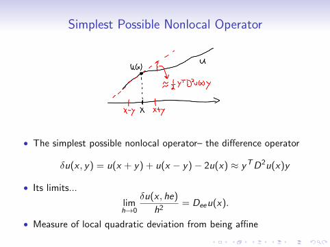
Simplest Possible Nonlocal Operator
• The simplest possible nonlocal operator– the difference operator
δu(x , y) = u(x + y) + u(x − y)− 2u(x) ≈ yTD2u(x)y
• Its limits...
limh→0
δu(x , he)
h2= Deeu(x).
• Measure of local quadratic deviation from being affine

Spherical Averages
• Infinitesimal weighted spherical average deviation from affine
∆u(x) = n limr→0
1
r 2
(1
|∂Br |
∫∂Br
δu(x , y)dSr (y)
)

Spherical Averages
• Average deviation from affine at all scales
−(−∆)α/2u(x) = C (n, α)
∫ ∞0
r−1−α(
1
|∂Br |
∫∂Br
δu(x , y)dSr (y)
)dr
• Rewritten as
−(−∆)α/2u(x) = C (n, α)
∫Rn
δu(x , y) |y |−n−α dy

Non-Spherical Averages
• Anisotropic averages in direction and scale, non-constantcoefficients weight K (x , y)
LK (u, x) = C (n, α)
∫Rn
δu(x , y)K (x , y)dy
note these LK do necessarily not satisfy LK (u(r ·), x) = rαLK (u, rx)!

Limits α→ 2
• Fractional Laplace → Laplace... C (n, α) ≈ (2− α) as α→ 2
∆u(x) = C (n) limα→2
(2− α)
∫Rn
δu(x , y) |y |−n−α dy
• Tr(AD2u(x)) = (∆u(√
A ·))((√
A)−1x)
Tr(AD2u(x)) = limα→2
(−(−∆)α/2u(√
A ·))((√
A)−1x)

Fully Nonlinear Equations– Ellipticity
• An example of general fully nonlinear operator F (u, x)
F (u, x) = infα
supβ
Cn,α
∫Rn
δu(x , y)Kαβ(x , y)dy.
• Choice of family in inf and sup =⇒ choice of ellipticity class,K a ∈ A , maximal and minimal operators with respect to A(Caffarelli, Caffarelli-Silvestre)
M−A(u, x) = infK a∈A
(LK a(u, x)) and M+A(u, x) = sup
K a∈A(LK a(u, x))
• F is elliptic with respect to A if
M−A(u − v , x) ≤ F (u, x)− F (v , x) ≤ M+A(u − v , x)

Fully Nonlinear Equations– Ellipticity
What does it mean to be uniformly elliptic, anyway? It’s worth somediscussion!
• A = K : (2−α)λ
|y |n+α ≤ K (x , y) ≤ (2−α)λ
|y |n+α – Caffarelli-Silvestre
• A = K = yTA(x)y
|y |n+α+2 : Tr(A) ≥ λ, 0 ≤ A(x) ≤ ΛId– Guillen-Schwab
• A = K :g( y
|y| )
|y |n+α ≤ K (x , y) ≤ Λ|y |n+α – Kassmann-Mimica
(g : Sn−1 → [0,∞) satisfies for some (symmetric) open subsetI ⊂ Sn−1 a uniform positivity assumption g ≥ δ > 0 on I )
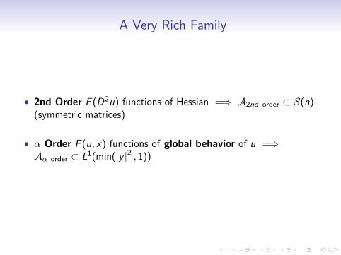
A Very Rich Family
• 2nd Order F (D2u) functions of Hessian =⇒ A2nd order ⊂ S(n)(symmetric matrices)
• α Order F (u, x) functions of global behavior of u =⇒Aα order ⊂ L1(min(|y |2 , 1))

A Very Basic Question

A Very Basic QuestionSuppose L is a “uniformly elliptic” (2nd or α order) and
Luk ≤ fk in B1
uk = 0 in Rn \ B1,
where for simplicity we assume uk ≤ 0 and 0 ≤ fk ≤ 1.
A Very Basic Question
When does |fk > 0| → 0 also imply inf(uk)→ 0?
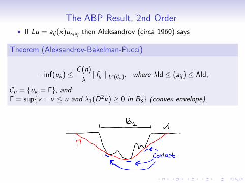
The ABP Result, 2nd Order
• If Lu = aij(x)uxixj then Aleksandrov (circa 1960) says
Theorem (Aleksandrov-Bakelman-Pucci)
− inf(uk) ≤ C (n)
λ‖f +
k ‖Ln(Cu), where λId ≤ (aij) ≤ ΛId,
Cu = uk = Γ, andΓ = supv : v ≤ u and λ1(D2v) ≥ 0 in B3 (convex envelope).

What About Integro-Differential Equations?
For L integro-differential (order α), until recently there was no answer.

The New ABP Result, α order
• A restricted family:
(LA)u(x) = C (n, α)
∫Rn
δu(x , y)(yTA(x)y) |y |−n−α−2 dy
• The minimal operator
M−(u, x) = inf(LA)u(x) : 0 ≤ A ≤ ΛId and Tr(A) ≥ λ
• These K (x , y) = yTA(x)y |y |−n−α−2 do not satisfy
λ
|y |n+α ≤ K (x , y) ≤ Λ
|y |n+α

The New ABP Result, α orderAssume that u is asupersolution
M−(u, x) ≤ f in B1
u ≥ 0 in Rn \ B1.
Theorem (Guillen-Schwab 2011)
− inf(u) ≤ C (n, α)
λ(‖f +‖L∞(Cu))(2−α)/2(‖f +‖Ln(Cu))α/2,
where Cu = u = Γα and Γα is an appropriate replacement for theconvex envelope, and C (n, α) is uniformly bounded as α→ 2.

Other Uses For The ABP

ABP in Homogenization
• Linear Equation simply for presentation
• φ fixed test function. Must find a unique λ such that the solutionv ε (in x variable) ∫δφ(x0, y)K ( xε , y , ω)dy +
∫δv ε(x , y)K ( xε , y , ω)dy = λ in B1(x0)
v ε = 0 in Rn \ B1(x0)
also satisfies as ε→ 0maxB1
|v ε| → 0
• If so, then F (φ, x0) = λ

ABP in Homogenization
(λ << 0
)λ = ?????
(λ >> 0
) ∫
δφ(x0, y)K ( xε , y , ω)dy +∫δv ε(x , y)K ( xε , y , ω)dy = λ in B1(x0)
v ε = 0 in Rn \ B1(x0)
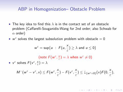
ABP in Homogenization– Obstacle Problem
• The key idea to find this λ is in the contact set of an obstacleproblem (Caffarelli-Souganidis-Wang for 2nd order; also Schwab forα order)
• w ε solves the largest subsolution problem with obstacle = 0
w ε = supu : F (u,x
ε) ≥ λ and u ≤ 0
(note F (w ε, xε ) = λ when w ε 6= 0)
• v ε solves F (v ε, xε ) = λ
M−(w ε − v ε, x) ≤ F (w ε,x
ε)− F (v ε,
x
ε) ≤ 1wε=0(x)F (0,
x
ε),

ABP in Homogenization– Obstacle Problem
M−(w ε − v ε, x) ≤ F (w ε,x
ε)− F (v ε,
x
ε) ≤ 1wε=0(x)F (0,
x
ε),
ABP =⇒ −(w ε − v ε) ≤ C |w ε = 0|1/n
So if |w ε = 0| → 0 as ε→ 0, then we know lim supε→0
v ε ≤ 0

ABP in Regularity– Point To Measure Estimate
Lemma (Point To Measure Estimate)
There are positive constants M > 1, µ < 1 and δ0 such that if u satisfies:
1. u ≥ 0 in Rn
2. infQ3
u ≤ 1
3. M−(u, x) ≤ f in Q4√n and ‖f ‖Ln(Q4
√n) ≤ δ0, ‖f ‖L∞(Q4
√n) ≤ 1.
Then we have the bound
|x ∈ Q1 : u(x) ≤ M| ≥ µ|Q1|.

ABP in Regularity– Point To Measure Estimate
Proposition (A Special Bump Function)
Given 0 < λ ≤ Λ and σ0 ∈ (0, 2) there exist constants C0,M > 0 and aC 1,1 function η(x) : Rn → R such that
1. supp η ⊂ B2√n(0)
2. η ≤ −2 in Q3 and ‖η‖∞ ≤ M
3. For every σ > σ0 we have M+(η, x) ≤ C0ξ everywhere where ξ is acontinuous function with support inside B1/4(0) and such that0 ≤ ξ ≤ 1.

ABP in Regularity– Point To Measure Estimate
• M−(u + Φ) ≤ f + ξ
• −1 ≤ − inf(u + Φ) ≤ C (‖f ‖α/2Ln +
∣∣∣u + Φ = Γ⋂
Q1
∣∣∣1/n)

Caffarelli-Silvestre Replacement For ABP
Assume that u is asupersolution
M−(u, x) ≤ f in B1
u ≥ 0 in Rn \ B1.
Theorem (Caffarelli-Silvestre 2009)
− inf(u) ≤ C (n, α)
λ
(∑i
(maxQif +)n
)1/n
where Qi is a finite cube covering of the contact set with the convexenvelope, Γ and C (n, α) is uniformly bounded as α→ 2.∣∣∣∣y ∈ √nQi : u(y) < Γ(y) + C (max
Qi
f )d2i ∣∣∣∣ ≥ µ |Qi |

Other Uses For 2nd Order ABP
A vital role for the 2nd order ABP
• Comparison of strong solutions for linear non-divergence equations
• Krylov-Safonov Harnack Inequality
• Fully Nonlinear Regularity Theory (Harnack and Holder)...Krylov-Safonov, Caffarelli, etc...
• W 2,ε estimates for Fully Nonlinear Equations... Fang-Hua Lin,Caffarelli, etc...
• (and things using the W 2,ε: Rates of convergence in numericalapproximations and homogenization, Caffarelli-Souganidis)
• Lp theory for viscosity solutions of fully nonlinear equations,Caffarelli-Crandall-Kocan-Swiech
• Stochastic Homogenization, Papanicolaou-Varadhan,Caffarelli-Souganidis-Wang
• many more...

Ideas of The Proof of The New ABP

A 120 Second Proof of The Original ABP (2nd Order)
• C is a cone chosen so that ∂C(0) ⊂ ∇Γ(B1) and inf C = −2M
c(n)Mn ≤ |∇Γ(B1)| ≤(change vars)
∫B1
det(D2Γ)dx
≤(λ1(D2Γ)=0)
∫u=Γ
det(D2Γ)dx ≤(det(D2Γ)1/n=inf(Tr(AD2Γ)))
∫u=Γ
(LΓ(x))ndx
≤(comparison)
∫u=Γ
(Lu(x))ndx ≤(equation)
∫u=Γ
(f +(x))ndx

New Difficulties (Headaches)
• convex envelope not compatible with integro-differential operators.
det(D2Γ(x)) (≤????) (M−(Γ, x))n
• u(x) = 1− |x |β with 0 < α < β < 1, u = Γ = 0, so estimatewill never hold
• reduction to u = Γ will not imply M−(Γ, x) ≤ 0... hence can’t getback to M−u and f

The Main Idea
• Replace Γ by a new envelope, Γα, TBD
• Raise the order of the equation• in principle Γα solves α-order equation• only know geometric arguments for 2nd-order equation• use Riesz Potential of Γα
P = Γα ∗ K where K (y) = A(n, 2− α) |y |−n+(2−α)
• 2nd order operations on P “should” give α-order operations on Γα
(−∆)P = (−∆)1(−∆)(α−2)/2Γα = (−∆)α/2Γα
• 2nd order proof on P “should” become compatible with M−(Γ, ·)

The New Tools
All new tools come from the following formula which is the correctversion of the incorrect (but useful) idea that we “should” have
Pxixj “ = ”Γα ∗ (Kyiyj ).
Lemma (formula for D2P)
D2P(x) =
(n + α− 2)(n + α)
2A(n, 2− α)
∫Rn
δΓ(x , y)
[y ⊗ y
|y |n+σ+2− Id
(n + σ) |y |n+σ
]dy .
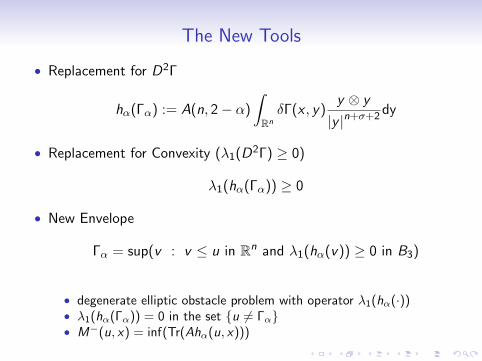
The New Tools
• Replacement for D2Γ
hα(Γα) := A(n, 2− α)
∫Rn
δΓ(x , y)y ⊗ y
|y |n+σ+2dy
• Replacement for Convexity (λ1(D2Γ) ≥ 0)
λ1(hα(Γα)) ≥ 0
• New Envelope
Γα = sup(v : v ≤ u in Rn and λ1(hα(v)) ≥ 0 in B3)
• degenerate elliptic obstacle problem with operator λ1(hα(·))• λ1(hα(Γα)) = 0 in the set u 6= Γα• M−(u, x) = inf(Tr(Ahα(u, x)))

The Picture
• M−Γα(x) ≤ M−(u, x) in the set u = Γα by comparison
• λ1(hα(Γα)) = 0 in the set u 6= Γα
• −(−∆)P = −(−∆)α/2Γα

Key Points of The Proof
• An important feature of Γα is that D2P can be computed classically!
Proposition (Γα is Regularizing)
If u is C 1,1 from above in B1, then Γα is Hα/2(Ω) for each Ω ⊂⊂ B3.

Key Points of The Proof
Lemma (Relationship Between det(D2P) and M−(Γ))
If D2P(x) ≥ 0, then det(D2P(x))1/n ≤ 1
nM−(Γ, x)
Proof.
n det(D2P)1/n = infTr(AD2P) : det(A) = 1, A ≥ 0
≤ infTr(BD2P) : det(B) = 1, B = A +Tr(A)
αId, A ≥ 0
≤ inf 1
det(B)1/nTr(BD2P) : B = A +
Tr(A)
αId, A ≤ ΛId, Tr(A) ≥ αλ
≤ inf 1
αλTr(Ahα(Γ)) : A ≤ ΛId, Tr(A) ≥ αλ= C (n, α)
λM−(Γ)

Key Points of The Proof
PCE is convex envelope of P in BR , R depends only on α
Lemma (Reduction to The Good Contact Set)
D2PCE > 0 ⊂ u = Γα
Proof.
We note that D2PCE > 0 ⊂ D2P > 0⋂P = PCE.
• case 1, x 6∈ B3. ∆P(x) = −(−∆)α/2Γα(x) < 0 because Γα(x) = 0which is global max of Γα =⇒ P(x) 6= PCE (x)
• case 2, x ∈ B3⋂u 6= Γα. ∃ unit vector τ with τThα(Γα, x)τ = 0
from λ1(hα(Γα, x)) = 0. =⇒ Pττ (x) ≤ 0.

Key Points of The Proof
now we use the geometric argument on P
(− infBR
(P))n ≤ C (n)
∫D2PCE>0
det(D2PCE )dx
≤Lem & comparison
C (n)
∫u=Γα
det(D2P)dx
≤det−min op ordering
C (n)
λn
∫u=Γα
(M−(Γα)
)ndx
≤equation
C (n)
λn
∫u=Γα
(f +)n
dx.

Key Points of The Proof
But we did not get what we want!!!! Need to relate inf(P) back toinf(Γα). This relationship is not to be expected from the Riesz Potentialalone...
Proposition (inf(P) & inf(Γα) relationship)
Let x0 be such that Γ(x0) = infRnΓ. Then
− infRnP = − inf
B3
P ≥ C (n, α)(−Γ(x0))2/α
(1
2f (x0)
)(2−α)/α
.
Key idea is to estimate the number of bad rings, R∗k , with radius 2−k
where ∣∣∣y : Γα(x0 + y)− Γα(x0) > f (x0) |y |α⋂
Rk
∣∣∣ ≥ 1
2|Rk |
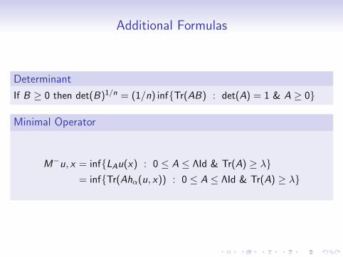
Additional Formulas
Determinant
If B ≥ 0 then det(B)1/n = (1/n) infTr(AB) : det(A) = 1 & A ≥ 0
Minimal Operator
M−u, x = infLAu(x) : 0 ≤ A ≤ ΛId & Tr(A) ≥ λ= infTr(Ahα(u, x)) : 0 ≤ A ≤ ΛId & Tr(A) ≥ λ

Open Problems
• More general kernels (cf. Kassmann-Mimica 2011)
g( y|y |)
|y |n+α ≤ K (x , y) ≤ Λ
|y |n+α ,
where g : Sn−1 → R satisfies for some open subset I ⊂ Sn−1 auniform positivity assumption g ≥ δ > 0 on I .
• Remove the interpolation form... find some p depending on α and n
− inf(u) ≤ C (n, α)
λ‖f +‖Lp
• W s,ε estimates(∫B1/2
∫Rn
|u(x + y) + u(x − y)− 2u(x)|ε
|x − y |n+sε
)1/ε
≤ C (‖u‖L∞+‖f ‖Lq)

The End
Thanks!