7

TSE‐466

OligopolyIntermediation,RelativeRivalry,andtheModeofCompetition

StephenF.Hamilton,PhilippeBontemsandJasonLepore

October2013

Oligopoly Intermediation, Relative Rivalry,

and the Mode of Competition

Stephen F. Hamilton∗

California Polytechnic State University San Luis Obispo

Philippe Bontems

Toulouse School of Economics (GREMAQ, INRA, IDEI)

Jason Lepore

California Polytechnic State University San Luis Obispo

October 15, 2013

Abstract

Policy design in oligopolistic settings depends critically on the mode of com-

petition between firms. We develop a model of oligopoly intermediation that

reveals the mode of competition to be an equilibrium outcome that depends

on the relative degree of rivalry between firms in the upstream and downstream

markets. We examine two forms of sequential pricing games: Purchasing to stock

(PTS), in which firms select input prices prior to setting consumer prices; and

purchasing to order (PTO), in which firms sell forward contracts to consumers

prior to selecting input prices. The equilibrium outcomes of the model range be-

tween Bertrand and Cournot depending on the relative degree of rivarly between

firms in the upstream and downstreammarkets. Prices are strategic complements

and the equilibrium prices coincide with the Bertrand outcome when the mar-

kets are equally rivalrous, while prices are strategic substitutes when the degree

of rivalry is sufficiently high in one market relative to the other. Cournot out-

comes emerge under circumstances in which prices are strategically independent

in either the upstream or downstream market. We derive testable implications

for the mode of competition that depend only on primitive conditions of supply

and demand functions.

JEL Classification: L13, L22, F13

Keywords: Oligopoly; Intermediation; Strategic Pre-commitment; Policy.

∗Correspondence to: S. Hamilton, Department of Economics, Orfalea College of Business, Cal-ifornia Polytechnic State University, San Luis Obispo CA 93407. Voice: 805-756-2555, FAX: 805-

756-1471, email: shamilto@calpoly.edu. Part of this paper was written while Stephen F. Hamilton

was visiting the Toulouse School of Economics and the author thanks members of that department

for their hospitality. We are indebted to Robert Innes and Richard Sexton for invaluable advise on

an earlier draft of the paper, and thank seminar participants at UC Berkeley, Toulouse School of

Economics, the University of Nebraska and the University of Kiel for helpful comments.

1

1 Introduction

An obstacle to deriving policy implications from the oligopoly model is the sensitiv-

ity of strategic pre-commitment devices to the mode of competition. As observed by

Fudenberg and Tirole (1984) and Bulow, Geanakoplos, and Klemperer (1985), the

strategic underpinnings of the oligopoly model depend fundamentally on the manner

in which firms’ choice variables alter the marginal profit expressions of rivals, a feature

that has essential implications for the design of effective policy. For strategic trade

policy, export subsidies are optimal when firms’ choice variables are strategic sub-

stitutes (Brander and Spencer 1985); however, export taxes are optimal when firms’

choice variables are strategic complements (Eaton and Grossman 1986). For strategic

delegation between the owner and manager of a firm, the optimal contract overcom-

pensates sales when firms compete in strategic substitutes, but overemphasizes cost

when agents compete in strategic complements (Fershtman and Judd 1987, Sklivas

1987). For contracts between vertically-aligned suppliers, the optimal contract in-

volves lump sum transfers from manufacturers to retailers when retailers compete

in strategic complements (Shaffer 1991), but involves negative lump sum payments

when retailers compete in strategic substitutes (Vickers 1985).1

In this paper, we develop a model of oligopoly intermediation that generates

testable hypotheses on the mode of competition. We frame our model around duopoly

intermediaries who purchase an input from a common upstream market and sell fin-

ished goods in a common downstream market. Both the input and output prices

selected by oligopoly firms are strategically interdependent, so that a pricing strat-

egy pursued by a firm in one market, for instance a price promotion on the finished

good designed to increase market share, has implications for both the supply and

demand conditions facing the rival. The intermediated oligopoly model provides a

convenient way to represent strategic interaction between firms: It reduces to the

1The mode of competition of the oligopoly model also has important implications for first-mover

advantage in sequential games between firms. It has been recognized since von Stackelberg (1934)

that advantage goes to the first-mover when choice variables are strategic substitutes; however, being

the first-mover is disadvantageous when firms compete in strategic complements (Gal-Or 1985).

2

usual oligopoly (oligopsony) model when the supply (demand) function is infinitely

elastic, yet encompasses general forms of strategic interaction when prices are inter-

dependent in both supply and demand functions.

We characterize the strength of the oligopoly pricing interaction between firms

in the upstream and downstream markets in terms of the degree of market rivalry.

The products procured and produced in each market are differentiated, as would be

the case when manufacturers rely on specialized inputs to produce branded consumer

goods, and a greater extent of product differentiation softens the degree of market ri-

valry. Our setting thus extends Stahl’s (1988) analysis of the intermediated oligopoly

model to differentiated product markets. We follow Stahl (1988) in examining two

forms of sequential price competition: (i) “purchasing to stock” (PTS), in which the

firms select input prices prior to setting output prices; and (ii) “purchasing to order”

(PTO), in which the firms sell forward contracts to consumers prior to selecting input

prices.

Our observations on the mode of competition depend critically on the “relative

degree of market rivalry” in the upstream and downstream markets. We define the

relative rivalry of the upstream market to be the difference (in absolute terms) be-

tween the ratio of the cross-price to own-price elasticity of supply and the ratio of

cross-price to own-price elasticity of demand. It is a measure of the relative strength

of the oligopoly interaction at each point of market contact between firms. If the

cross-price elasticity is zero in a market (the monopoly case), the market is non-rival,

whereas if the ratio of cross-price elasticity to own-price elasticity is approximately

one in a market (the case of commoditized products), the market is highly rival-

rous. Markets are equally rivalrous when there is no difference in the intensity of the

oligopoly interaction in the upstream and downstream markets, as would be the case

in the homogeneous product setting considered by Stahl (1988).

Our main results can be summarized as follows. First, we find that an outcome

of Bertrand merchants emerges only under circumstances in which the upstream and

downstream markets are equally rivalrous. Such an outcome occurs irrespective of

3

the degree of product differentiation in each market. Thus, our analysis reveals the

underpinning of the Stahl (1988) outcome of Bertrand merchants to be determined

by the relative degree of market rivalry rather than the absolute degree of rivalry in

the upstream and downstream markets.

Second, we show firm profits to be greater under PTS than under PTO when

the downstream market is relatively rivalrous, whereas the PTO outcome Pareto

dominates the PTS outcome in terms of firm and industry profits when the upstream

market is relatively rivalrous. In either case, setting prices in the less rivalrous market

serves as a pre-commitment device for prices in the more rivalrous market, providing

firms with the ability to soften price competition in the market where the degree of

oligopoly interaction is most intense.

Third, we demonstrate that when one market is more rivalrous than the other,

prices can be either strategic complements or strategic substitutes depending on the

relative degree of market rivalry. As the relative degree of market rivalry increases,

the equilibrium outcome under PTS and PTO converges to Cournot as prices be-

come strategically independent in the less rivalrous market. For the PTS game, this

result relates to the finding of Kreps and Scheinkman (1983) that the Cournot out-

come emerges in a two-stage game where firms first choose capacity and then select

prices. In general, the PTS game differs from the setting considered by Kreps and

Scheinkman (1983) in the sense that firms’ supply function in the upstream input

(capacity) market have rival’s input prices as arguments; however, the models are

isomorphic when each firm has monopsony control of an independent upstream mar-

ket.

Fourth, we provide conditions under which our observations on oligopoly inter-

mediation are robust to inventory-holding behavior in symmetric markets with linear

supply and demand functions. Our analysis thus formally extends the finding of Kreps

and Scheinkman (1983) to markets with differentiated products and interdependent

upstream markets.

Finally, we expand our analysis of sequential pricing outcomes to an extended

4

game in which firms first choose the timing of pricing decisions prior to selecting

prices. For the case of symmetric markets with linear supply and demand functions,

we verify that the Pareto dominant outcomes in the pricing sub-game represent equi-

librium strategies in the extended game. Namely, under circumstances in which

industry profits are largest under PTS (PTO), we show that such a pricing strategy

is also the equilibrium outcome of the extended game.

Our observations are related to previous research by Maggi (1996) that endog-

enizes the mode of competition in the oligopoly model.2 In Maggi’s (1996) model,

firms make capacity commitments before trading occurs in a downstream interna-

tional market, but can subsequently relax their prior capacity commitments subject

to an ex post adjustment cost parameter. This sequential capacity adjustment process

produces a continuum of outcomes that spans the modes of competition between

Bertrand and Cournot according to the cost of capacity adjustment. Our model de-

parts from this framework by specifying oligopsony interaction in the input (capacity)

market in place of ex post adjustment cost. An advantage of our approach is that it

results in testable hypotheses on the mode of competition that are readily estimable

from market data.

We illustrate the policy implications of the model for the case of a contract be-

tween a principle (a domestic trade authority, a firm, or a controlling shareholder)

and an agent (a domestic firm, a supplier/consumer, or a manager) that imposes a

unit tax or subsidy on the input procured from the upstream market. We show that

the optimal contract to maximize oligopoly profits involves taxing the input when

the upstream and downstream markets are relatively equal in terms of rivalry, but

subsidizing the input when the degree of relative rivalry is sufficiently large. We

numerically characterize these policy outcomes for perturbations in the relative de-

gree of market rivalry under linear supply and demand conditions and show that the

optimal value of the policy variable follows an inverted u-shaped pattern: As the

2We follow the convention of Maggi (1996) in characterizing the mode of competition according

to whether prices are strategic substitutes or strategic complements in the oligopoly model.

5

upstream market becomes increasingly rivalrous, the optimal policy switches from a

subsidy to a tax under PTS before reverting back to a subsidy under PTO.

The remainder of the paper is structured as follows. In the next Section we present

the model and characterize equilibrium prices under PTS and PTO. In Section 3, we

compare the outcomes for firm and industry profits and classify the Pareto domi-

nant Nash equilibrium according to the relative degree of rivalry in the upstream and

downstream markets. In Section 4, we extend these outcomes to consider inventory-

holding behavior and games with endogenous timing under symmetric market condi-

tions with linear supply and demand functions. In Section 5, we derive the mode of

competition in the linear model and characterize conditions for prices to be strategic

substitutes that depend only on observed market prices and estimable supply and

demand elasticities in a given industry. In Section 6, we numerically illustrate the

implication of our findings for the case of vertical contracts between firms and their

upstream suppliers, and in Section 7, we conclude. The proofs of all Propositions

appear in the Appendix.

2 The Model

We consider duopoly intermediaries who compete against each other in prices. The

firms purchase differentiated stocks (“inputs”) from suppliers in an upstream market,

and sell finished products (“outputs”) derived from the inputs to consumers in a

downstream market. Both input suppliers and consumers are price-taking agents in

their respective markets.

To clarify the implications of the model for oligopoly pricing outcomes, we consider

fixed proportions technology. Specifically, letting xi denote the quantity of the input

purchased in the upstream market by firm i ∈ 1, 2, we scale units such that yi = xidenotes the quantity of the output sold by the firm in the downstream market under

circumstances where inventory is not held. Products in each market are differentiated,

and the degree of rivalry between firms potentially differs at their points of contact

in the upstream and downstream markets according to the intensity of cross-price

6

effects between firms in each market. One interpretation of the nature of product

differentiation in the model is that demand and supply functions depend on the

spatial location of suppliers, consumers, and firms. Another interpretation is that

the firms require specialized inputs to produce differentiated consumer goods.

Let p = (p1, p2) denote the vector of output prices in R2. Consumer demand for

product i is given by

Di = Di(p), (1)

where Di is in the class of smooth functions on R2. We assume Dii ≡ ∂Di/∂pi < 0

and Dij ≡ ∂Di/∂pj ≥ 0, where the latter condition confines attention to the case

of substitute goods. We restrict output prices to P = [0, p] × [0, p], a convex andcompact subset R2, where p > 0 is a symmetric price such that Di(p, p) = 0 for all

p ≥ p and Di(p, p) > 0 for all p ∈ [0, p).Let w = (w1, w2) denote the vector of input prices. The supply function facing

firm i in the upstream market is

Si = Si(w), (2)

where Si is in the class of smooth functions on R2 and Sii ≡ ∂Si/∂wi > 0 and

Sij ≡ ∂Si/∂wj ≤ 0 (i.e., products in the upstream market are substitutes). As no

firm can earn positive rents with an input price greater than its output price, we

accordingly restrict input prices to be in P.

Throughout the paper, we assume that the direct effect of a price change outweighs

the indirect effect in each market; that is, ∆ ≡ DiiDjj −DijDji > 0 and Σ ≡ SiiSjj −SijS

ji > 0. These conditions ensure that the system of demand and supply equations

is invertible.

In Section 4.2, we derive sufficient conditions for no strategic inventory-holding

behavior. For now, we streamline the exposition of equilibrium outcomes under PTS

and PTO by suppressing inventory-holding behavior and the destruction or removal of

goods. Without the possibility of holding inventory, the demand and supply functions

7

facing each firm are linked by the material balance equations,

D(p) = S(w). (3)

There are two important subgames we define below: the PTS game and the PTO

game. In the PTS game, the two firms simultaneously and independently choose

their input prices. Given that the firms are not able to hold inventory, the unique set

of output prices associated with the input price pair w = (w1, w2) are determined by

condition (3), which we denote by p(w). Firm i’s profit in the PTS game is

πi,s(w) =¡pi(w)−wi

¢Si(w)− Fi, i ∈ 1, 2,

where Fi denotes fixed costs, a portion of which may be sunk.3

To guarantee existence and uniqueness of the PTS equilibrium, we impose the

following regularity conditions on profits.

Axiom 1 πi,sii (w) < 0, and π

i,sii (w) + π

i,sij (w) < 0 for all w ∈ P and i ∈ 1, 2.

In the PTO game, the two firms simultaneously and independently choose their

output prices. We assume that firms must fill all orders and cannot hold forward con-

tracts as inventory. As a consequence, the unique set of input prices are determined

by condition (3) under PTO as w(p). Firm i’s profit in the PTO game is

πi,o(w) =¡pi − wi(p)

¢Di(p)− Fi, i ∈ 1, 2,

We impose the following regularity condition on profits under PTO.

Axiom 2 πi,oii (p) < 0, and π

i,oii (p) + π

i,oij (p) < 0 for all p ∈ P and i ∈ 1, 2.

At times, we wish to compare equilibrium prices under PTS and PTO to those

that emerge under the “two-sided Cournot game” in which quantity choices deter-

mine both upstream and downstream market prices at once. To do so, we define

3 It is straightforward to show that continuity and differentiability of the the supply and demand

functions imply that πi,s is also in the class of smooth functions on R2.

8

inverse demand and inverse supply from equations (1) and (2) as P i(y) and W i(y),

respectively.

The profit of firm i under Cournot competition is given by

πi,C(y) =¡P i(y)−W i(y)

¢yi − Fi, i ∈ 1, 2, (4)

where y = (y1, y2) denotes the vector of retail (and wholesale) quantities under

quantity competition. To facilitate comparison of the PTS and PTO equilibrium

with the Cournot outcome, we make the following assumptions about the Cournot

profit functions.

Axiom 3 πi,Cii (y) < 0, and π

i,Cii (y)+π

i,Cij (y) < 0 for all y ∈ [0,D(0, p)]× [0,D(0, p)]

and i ∈ 1, 2.

This assumption guarantees existence and uniqueness of equilibrium in the Cournot

game. In addition, we assume that the collective profit is strictly concave in symmet-

ric quantities.

Axiom 4 πi,Cii (y) + 2π

i,Cij (y) + π

i,Cjj (y) < 0 for all symmetric y (y1 = y2).

As a convenient benchmark for this analysis, we first examine the case in which

firms simultaneously select prices in the upstream and downstreammarkets. Through-

out the paper, we refer to this object as the Bertrand outcome.

2.1 Bertrand Outcomes

Consider the case in which firms select prices simultaneously in the upstream and

downstream markets. Firm i seeks to maximize profits

πi,B(p,w) = piDi(p)− wiSi(w)− Fi, i ∈ 1, 2 (5)

subject to the inventory constraint (3). Evaluating the first-order conditions with

respect to wi and pi, we describe the Bertrand outcome in the sense of Stahl (1988)

as the simultaneous solution to

pi − wi = Si(w)

Sii(w)− D

i(p)

Dii(p), i ∈ 1, 2, (6)

9

where subscripts refer to partial derivatives.

Simultaneously solving equations (6) subject to the inventory constraint (3) yields

the Bertrand prices, which we define in the symmetric case as (wB, pB). For future

reference, it is helpful to express the symmetric price-cost margin of Bertrand mer-

chants as

pB − wB = pB

εdo+wB

εso. (7)

2.2 Relative Rivalry

The concept of relative rivalry is important for the analysis to follow. We define the

relative rivalry of markets as a measure of the strength of the oligopoly interaction

in the upstream market relative to the downstream market, where a more rivalrous

market is one in which a change in the input (output) price selected by a firm leads

to a greater change in supply (demand) for the rival. Focusing on the symmetric

market equilibrium, we describe the relative rivalry of markets in terms of supply

and demand elasticities. Specifically, let ²s =εscεso< 1 denote the absolute value of the

ratio of cross-price elasticity of supply (εsc = −Sij wjSi > 0) to own-price elasticity of

supply (εso = SiiwiSi> 0), and let ²d =

εdcεdo< 1 denote the corresponding ratio of demand

elasticities in the downstream market, where εdc = DijpjDi > 0 and εdo = −Dii piDi > 0.

Definition 1 The relative rivalry of the upstream market is given by Θ = ²s − ²d.

We measure the relative rivalry of the upstream market according to equilibrium

values for the prices in the Bertrand outcome described above. We refer to the

upstream market as being more rivalrous than the downstream market when Θ > 0,

the downstream market as being more rivalrous than the upstream market when

Θ < 0, and the markets as being equally rivalrous when Θ = 0.

We are now ready to examine the equilibrium outcomes of the intermediation

model under two forms of sequential pricing behavior: (i) Purchasing to Stock (PTS);

and (ii) Purchasing to Order (PTO).

10

2.3 Purchasing to Stock (PTS)

In the purchasing to stock (PTS) game, firms first select input prices and acquire

stocks in the upstream market, and then subsequently select output prices for finished

goods in the downstream market. Let w = (w1, w2) denote the vector of input prices

selected by the firms and let pi(w) and pj(w) denote the associated output prices

implicitly defined by equations (3).

Under PTS, firm i selects wi to maximize profits,

πi,s(wi, wj) =¡pi(w)− wi

¢Si(w)− Fi, i ∈ 1, 2, (8)

where Fi denotes fixed costs, a portion of which may be sunk. The first-order necessary

condition for a profit maximum is

πi,si ≡ (pi(w)− wi)Sii(w) + (pii(w)− 1)Si(w) = 0, i ∈ 1, 2. (9)

The effect of an input price change by firm i on output prices can be derived by

totally differentiating equations (3). Holding dwj = 0, this yields"Dii DijDji D

jj

# ∙dpidpj

¸=

∙SiiSji

¸dwi.

It follows that

pii(w) ≡∂pi

∂wi=DjjSii −DijSji∆

< 0

pji (w) ≡

∂pj

∂wi=DiiS

ji −DjiSii∆

. (10)

Equation (2.3) represents the own-price effect of an increase in the input price on the

output price of firm i. This term is negative. When firm i raises his input price, the

firm procures a greater quantity of the input, and this drives down the firm’s output

price and narrows his price-cost margin.

Equation (10) is the cross-price effect of a input price increase by firm i on the

output price of the rival firm j. The sign of this term is important for the results

to follow. Firm j responds to a higher input price by firm i (dwi > 0) by increasing

11

his output price (dpj > 0) whenever DiiSji > D

jiSii , and otherwise holds constant or

decreases his output price.

Under PTS, a change in a firm’s input price has two offsetting effects on the output

price of the rival. The first effect is the “supply effect”, DiiSji dwi ≥ 0. Selecting a

higher input price bids stocks away from the rival in the upstream input market,

which leads to an inward shift of the rival’s supply function. The supply effect

reduces the rival’s procurement of the input, thereby reducing the quantity sold in

the downstream market by firm j and raising the rival’s output price. The second

effect is the “demand effect”, DjiSiidwi ≥ 0. A rise in the input price of firm i raises

input procurement for firm i in the upstream market, leading to a commensurate

increase in production and sales for firm i in the downstream market and a decrease

in pi. The demand effect results in an inward shift of the rival’s demand function,

placing downward pressure on pj . The relative magnitude of the supply and demand

effects depends on the relative rivalry of the upstream market. When products in the

downstream market are commoditized, for example, the demand effect dominates the

supply effect, as total output would rise following a unilateral increase in the input

price of one firm, flooding the downstream market with finished goods.

In the symmetric market equilibrium (Di = Dj , Si = Sj , p1 = p2 = p,w1 = w2 =

w), the cross-price effect in equation (10) can be expressed in terms of relative rivalry

as

pji (w)

s= Θ,

where “s= ” denotes“equal in sign”. Under circumstances in which the upstream

market is relatively rivalrous (Θ > 0), an increase in the input price by firm i increases

the output price of firm j. When the downstream market is relatively rivalrous

(Θ < 0), an increase in the input price by firm i decreases the output price of firm j,

and for an equal degree of rivalry, Θ = 0, the output price of firm j is independent

of the input price selection of firm i.

Relative rivalry has essential strategic implications for the oligopoly model. To

12

see this, note that

Si(wi, wj) = Di(pi(w), pj(w))

under the inventory constraint (3). Differentiating this expression with respect to wi

and dropping arguments for notational convenience, we have

Sii = Diipii +D

ijpji .

When firm i increases his input price in the upstream market, this leads to a direct

increase in the output sold by firm i, Diipii > 0. But the input price increase also

facilitates a strategic response by the rival firm, Dijpji ≶ 0, the sign of which depends

on pji (and thus on Θ). Specifically, firm i perceives a smaller supply response to a

rise in wi when Θ < 0, which dampens the value of an input price increase. Thus,

engaging in PTS behavior serves as a commitment device to refrain from increasing

input prices when Θ < 0. It is of course in the interest of both firms to maintain lower

input prices in the upstream market, as this supports correspondingly higher output

prices in the downstream market and higher price-cost margins, making sequential

pricing behavior under PTS a facilitating practice whenever Θ < 0.

The equilibrium under PTS is determined by the simultaneous solution of equa-

tions (9). Let ws = (ws1, ws2) denote the equilibrium input price vector that solves

these equations and let ps = (ps1, ps2) denote the associated vector of equilibrium

output prices implied by equations (3).

The equilibrium price-cost margin for symmetric firms can be written

ps −ws = ks ps

εdo+ws

εso, (11)

where ks = 1+DjiD

jjΘ

∆. Notice that the second term on the right-hand side of equation

(11) is identical to the second term on the right hand-side of equation (7), but that

the first term differs from the Bertrand margin. Playing PTS introduces a weight on

the “demand-side” portion of the equilibrium price-cost margin that jointly accounts

for the relative rivalry of the upstream market. By inspection, ks > 1 if and only

if Θ < 0. That is, equilibrium price-cost margins are higher for firms in the PTS

13

game than in the Bertrand outcome when the upstream market is less rivalrous than

the downstream market (Θ < 0). The intuition for this finding is quite clear: When

Θ < 0, a decrease in the input price by a firm facilitates an increase in the rival’s

output price, thereby softening price competition in the downstream market.

In Section 3, we provide a more complete comparison of PTS and the Bertrand

outcomes. Before turning to this analysis, we derive the market equilibrium for the

remaining case of PTO.

2.4 Purchasing to Order (PTO)

Suppose the firms sell forward contracts for delivery of finished goods to consumers

prior to procuring inputs in the upstream market. Forward contracts are widely used

in practice, including imported goods sold to retail distributors and a significant

portion of wholesale trade (Stahl 1988).

Let p = (p1, p2) denote the vector of output prices selected by the firms and let

wi(p) and wj(p) denote the associated input prices defined by equations (3). In the

PTO game, firm i selects his output price to maximize profits of

πi,o(pi, pj) =¡pi − wi(p)

¢Di(p)− Fi, i ∈ 1, 2.

The first-order necessary condition for a profit maximum is

πi,oi ≡ (pi − wi(p))Dii(p) + (1− wii(p))Di(p) = 0, i ∈ 1, 2. (12)

We evaluate the PTO equilibrium by proceeding as above. Making use of the

implicit function theorem on equations (3) gives the input price responses

wii(p) ≡∂wi

∂pi=DiiS

jj −DjiSijΣ

< 0 (13)

wji (p) ≡

∂wj

∂pi=DjiSii −DiiSjiΣ

. (14)

Equation (13) measures the own-price effect of an increase in the output price, and

equation (14) measures the cross-price effect of a output price change by firm i on

the input price selected by firm j. As in the case of PTS, the sign of the cross-price

14

effect depends on the relative magnitude of the supply effect, DiiSji dpi ≥ 0, and the

demand effect, DjiSiidpi ≥ 0.

Notice that the cross-price effect in equation (14) always takes the opposite sign

of the cross-price effect in equation (10); that is, pji (w)

s= −wji (p). Under conditions

in which an increase in a firm’s input price increases the output price of his rival in

the PTS game, an increase in the output price decreases the input price of his rival

in the PTO game. In the symmetric market equilibrium (Di = Dj , Si = Sj , p1 =

p2 = p,w1 = w2 = w),

wji (p)

s= −Θ.

The equilibrium under PTO is determined by the simultaneous solution of equa-

tions (12). Define the equilibrium output price vector that solves these equations as

po = (po1, po2) and the associated vector of equilibrium input prices as wo = (wo1, w

o2).

The equilibrium price-cost margin for symmetric firms can be written

po −wo = po

εdo+ ko

wo

εso.

where ko = 1 − Sji S

jj

ΣΘ. Inspection of this term reveals that ko > 1 if and only if

Θ > 0. Equilibrium price-cost margins are higher in the PTO game than in the

Bertrand outcome when the upstream market is relatively rivalrous (Θ > 0). The

reason is that a rise in the output price by a firm decreases the input price set by his

rival when Θ > 0, which facilitates higher price-cost margins.

3 Equilibrium Outcomes

In this Section we compare firm profits in the PTS and PTO games to the Bertrand

outcome and identify Pareto dominant strategies in the symmetric market equilib-

rium. To do so, we consider the symmetric Bertrand prices (wB, pB) and examine

multilateral defections from the Bertrand outcome that increase the profits of firms.4

4With slight abuse of notation, we write demand, supply, and profit as functions of the scalar

values of input and output prices in the symmetric equilibrium.

15

3.1 PTS Versus PTO

Consider first the PTS game. Evaluating the input price condition (9) at the sym-

metric Bertrand values (wB, pB) gives

πi,si (w

B, pB) ≡ÃDjjSii −DijSji∆

− 1!Si −Di

µSiiDii

¶.

Making use of the market-clearing condition (3) and factoring terms yields

πi,si (w

B, pB) ≡ SiDijS

ii

∆Θ

s= Θ,

where all terms are evaluated at (wB, pB). In the PTS game, firms select higher input

prices than the symmetric Bertrand level when Θ > 0 and select lower input prices

when Θ < 0.

Proceeding similarly in the case of PTO, evaluating the output price condition

(12) at the symmetric Bertrand position (wB, pB) gives

πi,oi (w

B, pB) ≡ DiDiiS

ij

ΣΘ

s= Θ.

In the PTO game, firms select higher output prices than the symmetric Bertrand

level when Θ > 0 and set lower output prices when Θ < 0.

Proposition 1 For the intermediated oligopoly model:

(i) If Θ = 0 the equilibrium market outcome under either PTO or PTS is Bertrand

(ii) If Θ > 0 (< 0) the Pareto dominant equilibrium is PTO (PTS).

In Stahl’s (1988) model, intermediaries compete in homogeneous product markets

(Θ = 0), and an outcome with Bertrand merchants emerges under both PTO and

PTS. Proposition 1 extends this outcome to encompass any market that satisfies

Θ = 0. Thus, the Bertrand outcome represents an envelope of oligopoly equilibria

characterized by equal degrees of rivalry in the upstream market and downstream

market. The essential underpinning of the Bertrand outcome is that firms’ input

(output) price choices are independent of the resulting output (input) prices selected

16

by the rival. This outcome depends on the relative degree (rather than the absolute

degree) of market rivalry.

When Θ 6= 0, firm profits are larger in the symmetric equilibrium in cases where

the firms enjoy wider price-cost margins. Under circumstances where the downstream

market is relatively rivalrous (Θ < 0), the PTS game facilitates this outcome, because

the rival responds to a lower input price by selecting a higher output price in equation

(10). Equilibrium price-cost margins and profits are accordingly higher under PTS

than under Bertrand. Under circumstances where the upstream market is relatively

rivalrous (Θ > 0), profits are higher in the PTO game, as the rival firm responds

to a higher output price in this case by selecting a lower input price in equation

(14). In either case, the Pareto dominant equilibrium involves selecting prices in the

relatively less rivalrous market as a facilitating practice to soften price competition

in the remaining market.

The anatomy of the intermediated oligopoly model can be illustrated by describing

circumstances in which playing the PTS (PTO) game produces Cournot outcomes.

In the following section we characterize the Cournot equilibrium and derive formal

conditions under which the PTS and PTO games produce Cournot outcomes.

3.2 Cournot Outcomes

The Cournot outcome is characterized by maximizing expression (4) with respect to

yi. The first-order necessary condition for a maximum is

πi,Ci (y) = P i −W i +

µ∂P i

∂yi− ∂W i

∂yi

¶yi = 0, i ∈ 1, 2. (15)

Simultaneously solving equations (15) in the symmetric equilibrium gives the equilib-

rium quantity, yC = yC1= yC

2, which can be used to recover the symmetric Cournot

equilibrium prices (wC , pC).

Proposition 2 The Cournot outcome emerges in the PTS game when ²s = 0 and in

the PTO game when ²d = 0.

17

Proposition 2 clarifies the essential finding of Kreps and Scheinkman (1983) as an

outcome that depends on the strategic independence of prices in the upstream input

(capacity) market in the PTS game. The Cournot outcome also emerges in the PTO

game when the output prices of firms are strategically independent. In the following

section, we illustrate the robustness of these outcomes by considering circumstances

in which firms can hold inventories.

To see the intuition for Proposition 2, consider the price-cost margins under

Cournot in the symmetric market equilibrium. Making use of equations (2.3) and

(13), the symmetric equilibrium price-cost margin can be written as

pC − wC = pC

εdo¡1− ²2d

¢ + wC

εso (1− ²2s). (16)

The essential difference between this outcome and the outcome under PTS and

PTO is that quantity-setting firms jointly consider the strategic effect of a quantity

increase on raising their procurement cost in the upstream market and on reducing

their sales revenue in the downstream market. In contrast, firms in the PTS equilib-

rium, who set prices sequentially in the upstream market prior to selecting prices in

the downstream market, can consider only the implication of their first-stage input

price choice on their subsequent level of sales. When prices in the upstream market

are strategically independent, ²s = 0, however; the only interaction that remains with

the rival in this case occurs through the interdependence of prices in the downstream

oligopoly market, so that the inability of the firm to account for the strategic inter-

dependence of input prices in the upstream market no longer has any consequence.

When ²s = 0, the second term on the right-hand side of equation (16) reduces to wC

εso

and the weight on the demand-side portion of the equilibrium price-cost margin in

the PTS game reduces to ks = 11−²2

d

, resulting in the Cournot outcome. For a similar

reason, the PTO game results in the Cournot oligopsony outcome when prices are

strategically independent in the downstream market, ²d = 0.

18

4 Model Extensions

In this Section we consider two extensions of the model. We first extend the game

structure to a setting in which firms endogenously select the timing of their pricing

decisions from the choice set PTS, PTO prior to choosing prices. We then extendthe model to consider inventory-holding behavior by allowing the supply procured by

each firm to exceed demand in equations (3).

For each extension, we examine the symmetric market equilibrium under condi-

tions of linear supply and demand. Specifically, we consider the linear specialization,

Di(p) = maxa− bpi + cpj , 0, (17)

Si(w) = maxβwi − γwj , 0, (18)

where i = 1, 2, i 6= j, and where a, b,β > 0 and c, γ ≥ 0 are positive constants. Werestrict the each firm’s prices to the interval [0, P ], where P ≥ 2a/(b − c). Demand(supply) conditions reduce to local monopoly (monopsony) markets when c = 0 (

γ = 0) and products in the downstream (upstream) market become increasingly

commoditized as c −→ b (γ −→ β).

4.1 Endogenous Timing

Our observations above on the profit motive of firms to select prices sequentially

in intermediated oligopoly markets raises the question of whether such behavior is

also an equilibrium strategy in settings where coordination on timing is not possible

prior to selecting prices. Here, we extend the game structure to a setting in which

firms first choose whether to engage in PTS or PTO prior to selecting prices in each

market.

Consider the following three stage game. In stage 1, firms select the timing of

their pricing decisions from the choice set PTS, PTO. In stage 2, firms select pricesin the relevant subgame according to the timing of pricing decisions determined in

stage 1. The firms face symmetric market conditions in the second stage according

to the demand and supply functions in equations (17) and (18).

19

PTS2 PTO2

PTS1Sj

Sjj

− Dj

Djj

ks, Sj

Sjj

− Dj

Djj

ks Sj

Sjj

ko − Dj

Djj

, Sj

Sjj

− Dj

Djj

ks

PTO1Sj

Sjj

− Dj

Djj

ks, Sj

Sjj

ko − Dj

Djj

Sj

Sjj

ko − Dj

Djj

, Sj

Sjj

ko − Dj

Djj

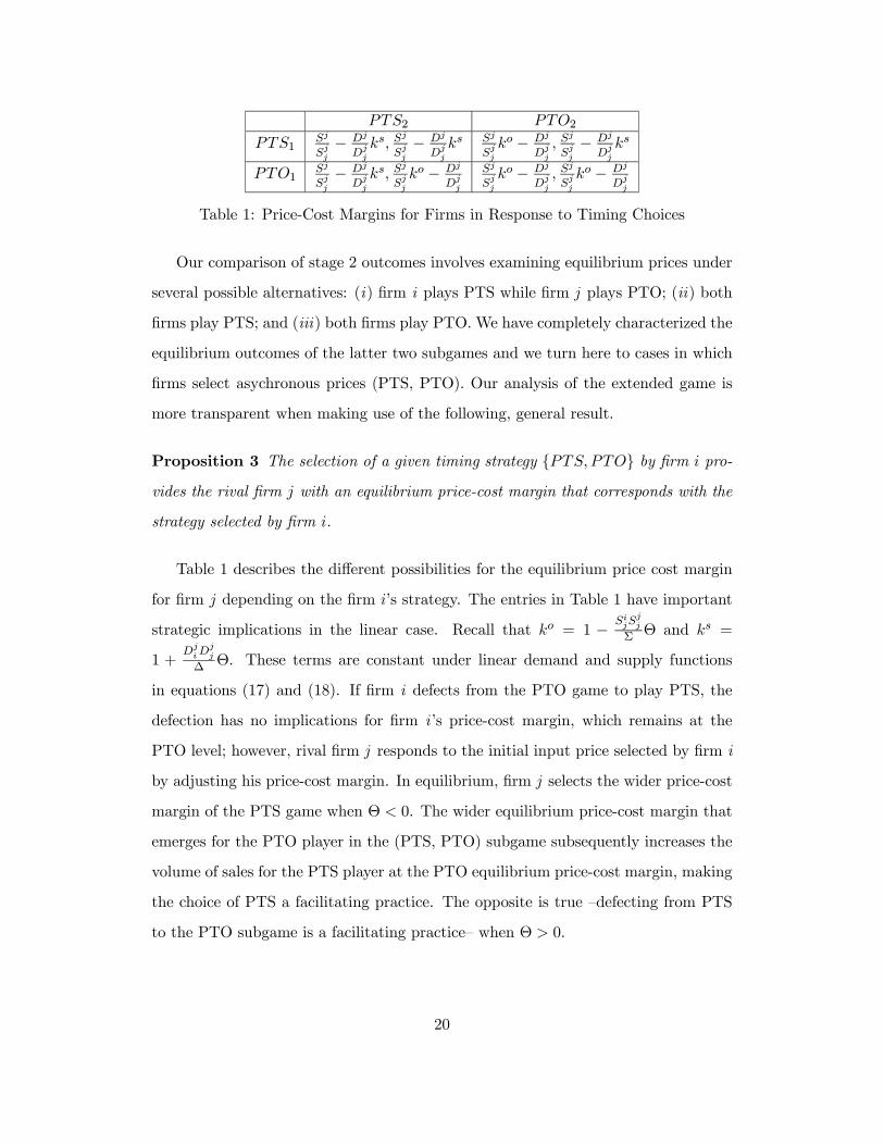
Table 1: Price-Cost Margins for Firms in Response to Timing Choices

Our comparison of stage 2 outcomes involves examining equilibrium prices under

several possible alternatives: (i) firm i plays PTS while firm j plays PTO; (ii) both

firms play PTS; and (iii) both firms play PTO. We have completely characterized the

equilibrium outcomes of the latter two subgames and we turn here to cases in which

firms select asychronous prices (PTS, PTO). Our analysis of the extended game is

more transparent when making use of the following, general result.

Proposition 3 The selection of a given timing strategy PTS, PTO by firm i pro-

vides the rival firm j with an equilibrium price-cost margin that corresponds with the

strategy selected by firm i.

Table 1 describes the different possibilities for the equilibrium price cost margin

for firm j depending on the firm i’s strategy. The entries in Table 1 have important

strategic implications in the linear case. Recall that ko = 1 − SijSjj

ΣΘ and ks =

1 +DjiD

jj

∆Θ. These terms are constant under linear demand and supply functions

in equations (17) and (18). If firm i defects from the PTO game to play PTS, the

defection has no implications for firm i ’s price-cost margin, which remains at the

PTO level; however, rival firm j responds to the initial input price selected by firm i

by adjusting his price-cost margin. In equilibrium, firm j selects the wider price-cost

margin of the PTS game when Θ < 0. The wider equilibrium price-cost margin that

emerges for the PTO player in the (PTS, PTO) subgame subsequently increases the

volume of sales for the PTS player at the PTO equilibrium price-cost margin, making

the choice of PTS a facilitating practice. The opposite is true —defecting from PTS

to the PTO subgame is a facilitating practice— when Θ > 0.

20

Now consider the outcome for profits under the system of equations (17) and (18).

Evaluating the symmetric pay-off matrix in the first stage of the game yields:

Proposition 4 Under linear supply and demand conditions:

(i) (Bertrand,Bertrand) is an equilibrium if and only if Θ = 0;

(ii) (PTS,PTS) is the unique equilibrium of the game when Θ < 0; and

(iii) (PTO,PTO) is the unique equilibrium of the game when Θ > 0.

The intuition for this result is that the choice of timing allows firms to employ

prices in the relatively less rivalrous market to serve as a facilitating practice to soften

price competition in the more rivalrous market. When Θ < 0, a firm that chooses

to play PTS causes his rival to adjust his price-cost margin upward in equilibrium,

because ks > 1. Moreover, as demonstrated by the entries in Table 1, this adjustment

occurs irrespective of the timing of price-setting behavior chosen by the rival firm.

The larger price-cost margin selected by the rival firm benefits the firm playing PTS,

and as a result, both firms select PTS in the first stage of the game. A comparable

outcome occurs when Θ > 0, allowing both firms to coordinate on PTO.

Before examining outcomes with inventory-holding behavior, it is worthwhile to

consider the case in which input prices are strategically independent in the upstream

market, ²s = 0. When ²s = 0, (PTS, PTS) is the unique equilibrium outcome in

the linear case and the margin adjustment by each firm is ks = 1 + (Dji )2/∆. The

unique equilibrium outcome of the game is Cournot. If the firms instead engaged in

PTO, ko reduces in this case to ko = 1, and the PTO equilibrium would produce

the Bertrand outcome. As in Kreps and Scheinkman (1983), the firms would wish to

defect from selecting output prices that result in Bertrand profits by first committing

to the purchase of stocks (“capacity”), which results in the Cournot outcome.

4.2 Inventory-Holding

Now consider a setting in which inventory-holding behavior is possible. For exposi-

tional clarity, we limit our attention to market conditions that satisfy Θ < 0, which

21

provides strategic incentives for PTS to emerge as the unique equilibrium outcome

in the case where holding inventory is not possible. Analogous conditions apply for

PTO in settings where forward contracts do not represent binding commitments to

deliver finished goods to consumers in the downstream market.5

Suppose stocks procured from the upstream input market in the PTS game can

be freely disposed. The possibility of free disposal of inputs relaxes the inventory

constraint in equation (3), which becomes Di(p) ≤ Si(w) for i = 1, 2.To study the pricing subgame with fixed supplies and potentially slack inventory

constraints, we follow Kreps and Scheinkman (1983) and assume that residual demand

is efficiently rationed. We then characterize the profitability of defection strategies

from the no-inventory equilibrium. This analysis results in the following:

Proposition 5 The inventory constraint in equation (3) is always binding when 6

P ij (y)Sji (w) ≤ 1 + εso. (19)

The implication of Proposition 5 is that the PTS equilibrium described above

under the assumption of no inventory-holding coincides with the equilibrium outcome

in a general setting with inventory-holding behavior provided that condition (19)

holds. The interpretation of this condition is as follows. After input procurement

has taken place, the procurement cost of the firm is sunk, leaving the firm with the

potential to sell less than the procured quantity with no additional cost under the

assumption of free disposal. Proposition 5 describes market conditions under which a

firm selecting quantities in a setting with no production cost would wish to select an

output level that is (at least weakly) greater than the output level implied by PTS,

thereby resulting in a binding inventory constraint.

5The possibility of holding negative inventory under PTO implicitly assumes that forward con-

tracts with consumers can be renegotiated. In the event that forward contracts are non-renegotiable,

free disposal of forward contracts would not be possible, and an additional deterrent would exist to

holding inventory under PTO.6 In the linear case, all terms in condition (19) are constant and the inequality can be written,

γc(β − γ) ≤ ∆(2β − γ), which holds for sufficiently “small” c, γ.

22

5 Mode of Competition

Characterizing and measuring the mode of competition in the oligopoly model is

essential for deriving policy prescriptions in settings with strategic pre-commitment.

It is also important for deriving inferences on the type of market conditions that

warrant antitrust scrutiny, for instance market features that favor the use of slotting

allowances as a practice to soften price competition.7 Our goal in this section is to

develop testable hypotheses on the mode of competition in industrial settings.

To characterize the mode of competition in intermediated oligopoly settings, con-

sider the second partials of profit under PTS. Dropping arguments for notational

convenience, the effect of an input price change by firm j on the marginal profit of

firm i under PTS is

πi,sij ≡ (pi −wi)Siij + (pii − 1)Sij + pijSii + piijSi, i ∈ 1, 2. (20)

Prices may be strategic complements (πi,sij > 0) or strategic substitutes (π

i,sij < 0) in

the sense of Bulow, Geanakoplos, and Klemperer (1985).

To provide an intuitive characterization of these outcomes, consider the first-order

effects in expression (20). Classifying the mode of competition in the linear model

is important for deriving testable hypotheses for empirical work that relies on linear

estimation techniques. On substitution of equations (2.3) and (10), the mode of

competition in the PTS game can be expressed as

πi,sij =

ÃDjjSii −DijSji∆

− 1!Sij +

ÃDjjSij −DijSjj∆

!Sii .

In the symmetric market equilibrium, this condition becomes

πsijs=(p− w)p

εdo²s¡1− ²2d

¢+Θ, (21)

where the first term on the right hand side of equation (21) is positive and Θ < 0 is

negative in the PTS game by Proposition 1. It can be seen immediately upon inspec-

tion of terms in equation (21) that prices are strategic complements when markets7The Federal Trade Commission (FTC), which regulates the grocery industry, refused to provide

guidelines for slotting allowances, citing the need for further investigation on the efficiency effects of

the practice (FTC 2001).

23

are equally rivalrous, Θ = 0 (Bertrand), whereas prices are strategic substitutes in

the case where prices are strategically independent in the upstream market, ²s = 0

(Cournot). In general, Θ < 0 is a necessary but not a sufficient condition for prices

to be strategic substitutes in the PTS game.

In the PTO game, the effect of an output price change by firm j on the marginal

profit of firm i is

πi,oij = (pi − wi − ti)Diij + (1− wii)Dij − wijDii − wiijDi, i ∈ 1, 2. (22)

Confining attention to first-order effects in expression (22) and making substitutions

from (13) and (14) in the symmetric market equilibrium yields

πoijs=(p−w)w

εso²d¡1− ²2s

¢−Θ. (23)

As in the PTS game, output prices may be strategic complements (πi,oij > 0) or

strategic substitutes (πi,oij < 0) depending on the magnitude of Θ > 0. When Θ > 0,

the first term on the right-hand side of the expression is positive and the second

term is negative. The relative rivalry of the upstream market influences the mode of

competition under PTO in the opposite manner as under PTS: The model reduces

to Bertrand when Θ = 0 and to Cournot oligopsony when ²d = 0. A relatively

rivalrous upstream market (Θ > 0) is necessary but not sufficient for output prices

to be strategic substitutes in the PTO game.

Proposition 6 Under conditions of linear supply and demand, prices are strategic

substitutes in the intermediated oligopoly model when:

(i) ²s ≤ ²dh1+

(p−w)p

εdo(1−²2d)i ; or

(ii) ²d ≤ ²sh1+

(p−w)w

εso(1−²2s)i .

Under circumstances in which Θ < 0 (²s < ²d), the upstream market is relatively

less rivalrous than the downstream market. Firms are able to soften downstream price

competition by selecting input prices prior to output prices in the PTS game. Part

24

(i) of Proposition 6 is the relevant criteria for the mode of competition, and prices

are strategic substitutes when ²s is sufficiently small relative to ²d. The opposite is

true when Θ > 0 (²d < ²s). Part (ii) of Proposition 6 is the relevant criteria for the

mode of competition, and prices are strategic substitutes when ²d is sufficiently small

relative to ²s. In either case, the mode of competition is determined by the relative

rivalry of the upstream market.

6 Policy Implications

The mode of competition in the oligopoly model has important implications in a num-

ber of policy settings. In this section, we highlight policy implications of the model

for the case of contract design between a principal (a domestic trade authority, a firm,

or a controlling shareholder) and an agent (a domestic firm, a supplier/consumer, or

a manager). For expositional clarity, we consider strategic policies by the principal

that tax or subsidize input procurement by the agent in the upstream market un-

der conditions of linear supply and demand. This allows us to numerically compute

the optimal tax level for variation in the relative rivalry of the upstream market by

perturbing c and γ in the system of equations (17) and (18).

We consider the following three-stage game. In stage 1, the principal of firm i

imposes a unit tax ti on inputs procured in the upstream market by agent i. In

stage 2, agents take principals’ policy decisions parametrically and select the timing

of pricing decisions, and in stage 3, agents select prices in the relevant subgame.

Letting πi(p,w) denote the profit of principal i, we denote agent i ’s profit

Πi(p,w) = πi(p,w)− tiSi(w) + Ωi, i ∈ 1, 2, (24)

where Ωi is a lump-sum transfer that subsumes fixed costs. Maximizing the agent’s

profit gives the first-order condition

Πi,si ≡

¡pi(w)− wi − ti

¢Sii(w) + (p

ii(w)− 1)Si(w) = 0, i ∈ 1, 2, (25)

for the PTS game and

Πi,oi ≡ (pi − wi(p)− ti)Dii(p) + (1− wii(p))Di(p) = 0, i ∈ 1, 2, (26)

25

for the PTO game.

Proposition 7 The choice of PTO or PTS as an equilibrium strategy of agent i is

invariant to the principal’s choice of policy variable ti. Thus, the market equilibrium

is Bertrand if Θ = 0, PTO if Θ > 0, and PTS if Θ < 0.

The magnitudes of the policy variables, ti, i = 1, 2 influence neither the sign

nor the value of Θ. An implication of Proposition 7 is that our observations on

strategic pre-commitment devices are robust to different policy structures that alter

the marginal returns facing oligopoly agents.

Confining attention to first-order effects, the second partial of Πi with respect to

wi and wj is

Πi,sij = p

ij(w)S

ii(w) + (p

ii(w)− 1)Sij(w) = π

i,sij , i ∈ 1, 2,

for the PTS game and the second partial of Πi with respect to pi and pj is

Πi,oij = (1− wii(p))Dij(p)−wij(p)Dii(p) = π

i,oij , i ∈ 1, 2.

In the symmetric market equilibrium, it is straightforward to show that the opti-

mal values of the policy variables satisfy

t∗is= π

i,sij

s= π

i,oij , i ∈ 1, 2.8 (27)

The optimal value of the policy variable for each agent depends on the mode of

competition between oligopoly firms. Taxes (t∗i > 0) are optimal when prices are

strategic complements, whereas subsidies (t∗i < 0) are optimal when prices are strate-

gic substitutes.

The intermediated oligopoly model allows the optimal value of the strategic pre-

commitment policy to be explicitly computed according to supply and demand con-

ditions facing firms. We illustrate this outcome for the case of linear supply and

demand functions by calculating the (unique) Nash equilibrium in policy variables

8Full derivation of the optimal policy varibles is provided in the Web Appendix.

26

for variation in the degree of pricing interdependence in each market, c and γ. For

our numerical analysis, we select parameters a = b = β = 1 and identify the optimal

tax policy in the symmetric pre-commitment equilibrium, t∗ = t∗i = t∗j for variations

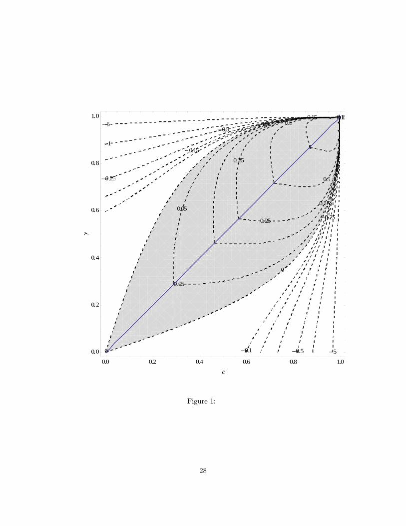
in c ∈ (0, 1] and γ ∈ (0, 1].Figure 1 depicts the contour lines of the symmetric trade policy equilibrium in

the space (c, γ). Note that PTS is the unique equilibrium of the game when γ > c,

while PTO is the unique equilibrium of the game when γ < c. The optimal trade

policy is a tax (t∗ > 0) in the shaded region of the figure and a subsidy (t∗ < 0) in

the non-shaded area of the figure. The contour line where the laissez-faire outcome

is optimal (t∗ = 0) is represented by the contour line that separates these two areas.

For a fixed γ (respectively c) the optimal policy reveals an inverted u-shaped pattern

as c (respectively γ) increases from 0 to 1.

7 Concluding Remarks

The oligopoly intermediation model results in testable hypotheses on the mode of

competition that can be used to derive policy implications in industrial settings. Our

analysis reveals the prevailing mode of competition in a particular industry to be

an empirical question that depends on estimable parameters of supply and demand

functions in the upstream and downstream markets where firms interact.

We have demonstrated that oligopoly firms have an incentive to select input prices

prior to choosing output prices in the PTS game when the downstream market is rel-

atively rivalrous, but to select output prices prior to choosing input prices in the

PTO game when the upstream market is relatively rivalrous. Under reasonably mild

conditions, we have shown these outcomes to be robust to the possibility of strategic

inventory-holding behavior of firms. For both the PTS and PTO games, prices are

strategic complements when the upstream market and the downstream market are

relatively equal in terms of rivalry, whereas prices are strategic substitutes under cir-

cumstances where the upstream (downstream) market is sufficiently rivalrous relative

27

-5

-5-1

-1

-0.5

-0.5

-0.25

-0.25

-0.15

-0.15

-0.1

-0.10

0

0.05

0.05

0.15

0.15

0.25

0.25

0.5

0.5

1

1

0.0 0.2 0.4 0.6 0.8 1.0

0.0

0.2

0.4

0.6

0.8

1.0

c

g

Figure 1:

28

to the remaining market. In the case where the markets are equally rivalrous, the

equilibrium outcome of the oligopoly model is Bertrand and in cases where prices are

strategically independent in either the upstream market or the downstream market,

the equilibrium outcome of the oligopoly model is Cournot.

Our model provides empirical direction for examining the mode of competition in

industrial settings that can be used to tailor pre-commitment policies to the particular

conditions facing firms. This feature of the model can provide a useful tool for policy

formulation as well as for the enforcement of anti-trust regulations in a given industry.

An interesting avenue for future research is to consider an active role for firms in

contributing to market rivalry through product differentiation. To the extent that

oligopoly firms engage in activities to differentiate themselves from rivals, whether by

creating differentiated products from common inputs or by discovering new techniques

for producing existing products from specialized inputs, differentiation can provide a

tool to soften price competition with rivals. But, perhaps surprisingly, our analysis

clarifies that relaxing market rivalry is not necessarily a globally desirable endeavor.

The reason is that it is the relative degree of market rivalry — not the absolute degree—

that is the source of strategic advantage. Indeed, a firm that seeks to specialize input

requirements would have a greater ability to soften price competition with rivals when

downstream products are commoditized than when downstream products are highly

differentiated. Our model suggests the potential for “strategic standardization” to

occur under circumstances in which inputs (outputs) in the upstream (downstream)

market are highly specialized.

29

References

[1] Bertrand, Joseph. 1883. “Theorie Mathematique de la Richesse Sociale,” Journal

des Savants: 499-508.

[2] Brander, James A. and Barbara J. Spencer. 1985. “Export Subsidies and In-

ternational Market Share Rivalry,” Journal of International Economics 18(1-2):

83-100.

[3] Bresnahan, Timothy F. 1981. “Duopoly Models with Consistent Conjectures,”

American Economic Review 71(5): 934-45.

[4] Bulow, Jeremy I., John D. Geanakoplos, and Paul D. Klemperer. 1985. “Multi-

market Oligopoly: Strategic Substitutes and Complements,” Journal of Political

Economy 93(3): 488-511.

[5] Cournot, Augustine. 1838. Recherches sur les Principes Mathematiques de la

Theorie des Richesses. Paris.

[6] Eaton, Jonathan and Gene M. Grossman. 1986. “Optimal Trade and Industrial

Policy under Oligopoly,” Quarterly Journal of Economics 101(2): 383-406.

[7] Fershtman, Chaim and Kenneth L. Judd. 1987. “Equilibrium Incentives in

Oligopoly,” American Economic Review 77(5): 927-40.

[8] Fudenberg, Drew, and Jean Tirole. 1984.“The Fat-Cat Effect, the Puppy-Dog

Ploy, and the Lean-and-Hungry Look,” American Economic Review 74(2): 361-

68.

[9] Gal-Or, Esther. 1985. “First Mover and Second Mover Advantages,” Interna-

tional Economic Review 26(3): 649-53.

[10] Kreps, David M. and Jose A. Scheinkman. 1983. “Quantity Precommitment and

Bertrand Competition Yield Cournot Outcomes,” Bell Journal of Economics

14(2): 326-37.

30

[11] Maggi, Giovanni. 1996. “Strategic Trade Policies with Endogenous Mode of Com-

petition,” American Economic Review 86(2): 237-58.

[12] Martin, Stephen. 1999. “Kreps And Scheinkman With Product Differentiation:

An Expository Note,” University of Copenhagen, Centre for Industrial Eco-

nomics Discussion Paper no. 1999-11.

[13] Shaffer, Greg. 1991. “Slotting Allowances and Resale Price Maintenance: A

Comparison of Facilitating Practices,” RAND Journal of Economics 22(1): 120-

36.

[14] Singh, Nirvikar and Xavier Vives. 1984. “Price and Quantity Competition in a

Differentiated Oligopoly,” RAND Journal of Economics 15(4): 546-54.

[15] Sklivas, Steven D. 1987. “The Strategic Choice of Managerial Incentives,” RAND

Journal of Economics 18(3): 452—458.

[16] von Stackelberg, Heinrich. 1934. Market Structure and Equilibrium (Marktform

und Gleichgewicht). 1st Edition Translation into English, Springer: Bazin, Urch

& Hill, 2011.

[17] Stahl, Dale O. 1988. “Bertrand Competition for Inputs and Walrasian Out-

comes,” American Economic Review 78(1): 189-201.

[18] Vickers, John. 1985. “Delegation and the Theory of the Firm,” Economic

Journal 95 (Supplement): 138-47.

[19] Vives, X. 1999. Oligopoly Pricing: Old Ideas and New Tools. (Cambridge: MIT

Press).

31

Appendix

A Proof of proposition 1

The proof is constructed by comparing equilibrium prices under PTO and PTS to

Bertrand prices and the prices that emerge from symmetric joint profit maximization.

The joint profit maximizing solution involves selecting a symmetric quantity pair

(y, y) to maximize

πM(y) =X

i∈1,2πi,C(y),

where πi,C(y) is given by expression (4). Collective profit, πM(y), is concave in the

symmetric quantities under Assumption 4. This is immediate since,

∂2πM(y)

∂y2=

Xi∈1,2

³πi,C11 (y) + 2π

i,C12 (y) + π

i,C22 (y)

´< 0

To complete the proof, we show that the prices that maximize collective industry

profits in the symmetric market equilibrium (pM , wM) satisfy wM < ws ≤ wB andpM > po ≥ pB. When this condition holds, firm profits are rising for defections from

wB (pB) that involve w < wB (p > pB) under PTS (PTO).

The first-order necessary condition for a joint profit maximum is

∂πM(y)

∂y≡ P i −W i +

µ∂P i

∂yi− ∂W i

∂yi

¶y +

µ∂P j

∂yi− ∂W j

∂yi

¶y = 0, i ∈ 1, 2, i 6= j

(28)

Simultaneously solving (28) for symmetric quantities yields yM(= yM1 = yM2 ), which

can be used to recover the joint profit maximizing prices.

To facilitate the comparison of the joint profit maximizing outcome with the

Bertrand, PTS, and PTO equilibria, note that ∂P i

∂yi=

Djj

∆< 0, ∂P j

∂yi=

−Dji

∆< 0,

∂W i

∂yi=

Sjj

Σ> 0 and ∂W j

∂yi=−SjiΣ> 0 for all prices in P. Incorporating these terms in

(28) and evaluating the slope of the joint profit function at the symmetric Bertrand

32

output level, yB, as defined by (pB − wB) = yB³1Sii− 1

Dii

´, gives

πMi (yB) = yB

⎡⎣ 1Sii− 1

Dii+Djj −Dji∆

−

³Sjj − Sji

´Σ

⎤⎦= yB

"Sji (S

ii − Sij)SiiΣ

+Dji (D

ij −Dii)Dii∆

#< 0.

Hence the output level that maximizes joint profits in the symmetric case satisfies

yM < yB. By concavity of πMi (y), it follows that wM < wB and pM > pB.

It remains to compare the joint profit maximization solution to the equilibrium

outcomes under PTS and PTO. Our conjecture is that profitable defections from the

Bertrand prices involve w < wB and p > pB. This conjecture holds provided that

wM < ws < wB and pM > po > pB. We have already demonstrated that firms select

ws < wB in the PTS game when Θ < 0 and that firms select po > pB in the PTO

game when Θ > 0. It remains to be shown that wM < ws and pM > po.

To verify this conjecture, consider the slope of the joint profit function at the

symmetric PTS equilibrium position, ys, as implicitly defined by equation (9): (ps−ws) = ys

Sii

µ1− (D

jjS

ii−Di

jSji )

∆

¶. Collecting terms in (28) yields

πMi (ys) =

ys

Sii

"1− (D

jjSii −DijSji )∆

#+ ys

⎛⎝Djj −Dji∆

−

³Sjj − Sji

´Σ

⎞⎠ .Factoring this expression yields

πMi (ys) =

ys³Sii − Sji

´Sii

"Sji

Σ− D

ji

∆

#< 0.

The output level that maximizes joint profits in the symmetric case satisfies yM < ys.

By concavity of πMi (y), it follows that wM < ws and pM > ps. Thus, wM < ws < wB

for Θ < 0.

Proceeding similarly in the case of PTO competition, evaluating the slope of

collective profit at the symmetric PTO equilibrium position gives

πMi (po, wo) =

y³Dii −Dij

´Dii

"Sji

Σ− D

ji

∆

#< 0.

33

By inspection, yM < yo, so that wM < wo and pM > po in the PTO game. It follows

that pM > po > pB for Θ > 0.

¤

B Proof of Proposition 2

First consider PTS. We wish to show that the PTS game produces Cournot outcomes

when ²s = 0. Note that ∂P i

∂yi=

Djj

∆< 0 and ∂W i

∂yi=

Sjj

Σ> 0 for all prices in P.

Incorporating these terms in optimality condition (15), the Cournot equilibrium is

characterized in the symmetric case by

πi,Ci (y) = P i −W i +

ÃDjj

∆− S

jj

Σ

!yi = 0. (29)

The proof is constructed by showing that the equilibrium condition under PTS coin-

cides with (29) when ²s = 0. Noting that ²s = 0 holds if and only if Sij = S

ji = 0,

condition (9) in the PTS game reduces to

πi,si ≡ (pi − wi)Sii +

ÃDjjSii

∆− 1!Si = 0⇔ pi − wi +

ÃDjj

∆− 1

Sii

!Si = 0.

To verify that the symmetric equilibrium in the PTS game produces Cournot out-

comes when ²s = 0, note that the Cournot equilibrium satisfies pC−wC =

µ1Sii− D

jj

∆

¶yC

when Sij = Sji = 0. Evaluating the first-order condition for the PTS game at the

Cournot equilibrium output level, Si = yC completes the proof.

Proceeding similarly for the case of PTO, note that ²d = 0 holds if and only if

Dij = Dji = 0, which reduces equilibrium condition (12) to

πi,oi ≡ (pi − wi)Dii +

Ã1− D

iiSjj

Σ

!Di = 0⇔ pi −wi +

Ã1

Dii− S

jj

Σ

!Di = 0.

When Dij = Dji = 0, the Cournot equilibrium satisfies pC − wC =

µSjj

Σ− 1

Dii

¶yC .

Evaluating the first-order condition from the PTO game at the Cournot equilibrium

output level, Di = yC completes the proof.

¤

34

C Proof of Proposition 3

The proof is constructed by sequentially evaluating the asynchronous pricing outcome

in the stage 2 subgame in which one firm plays PTS and the rival plays PTO.

Lemma 1. When firm i plays PTS and firm j plays PTO the equilibrium price-cost

margins are pi−wi = Si

Siiko−Di

Dii

and pj−wj = Sj

Sjj

−Dj

Djj

ks, where ko = 1− SijSjj

ΣΘ

and ks = 1 +DjiD

jj

∆Θ.

Proof. Totally differentiating the binding inventory constraints yields"Dii −SijDji −Sjj

# ∙dpidwj

¸=

"Sii −DijSji −Djj

# ∙dwidpj

¸,

and the corresponding responses

∂pi

∂wi=−SjjSii + SijSji−SjjDii + SijDji

= −ΣΨ< 0

∂wj

∂wi=

SjiD

ii − SiiDji

−SjjDii + SijDji= −D

jjSjjΘ

Ψ

s= Θ

∂pi

∂pj=

SjjD

ij − SijDjj

−SjjDii + SijDji=DiiS

iiΘ

Ψ

s= −Θ

∂wj

∂pj=−DjjDii +DijDji−SjjDii + SijDji

= −∆Ψ< 0

where Ψ = −SjjDii + SijDji > 0, Σ = SjjSii − SijSji > 0, ∆ = DjjDii −DijDji > 0 andusing symmetry, Θ =

SiiDji−SjiDi

i

DjjS

jj

.

Next, consider the problems of firms i and j in stage 1. The profit function for

firm i is

maxwi

πi,s =¡pi(wi, pj)− wi

¢Si(wi, w

j(wi, pj)),

with the corresponding first-order necessary condition

¡pi(wi, pj)− wi

¢µSii + S

ij

∂wj

∂wi

¶+

µ∂pi

∂wi− 1¶Si = 0.

35

Factoring this expression and making use of the inventory constraint gives

pi − wi = Si

Sii

ÃSii

Sii

!− D

i

Dii

Ã−D

iiΣ

SiiΨ

!

with Sii = Sii − Sij

DjjS

jjΘ

Ψ. Expanding terms, we have

−DiiΣ

SiiΨ=

−Dii³SjjS

ii − SijSji

´Sii

³−SjjDii

´+ Sij

³SjiD

ii

´ = 1and

Sii

Sii=

SiiΨ

Dii

³SijS

ji − SiiSjj

´ = −SiiΨDiiΣ

= 1− SijSjj

ΣΘ.

Substitution of terms yields the equilibrium price-cost margin of firm i :

pi −wi = Si

Siiko − D

i

Dii.

The profit function of firm j is

maxpj

πj,o =¡pj − wj(wi, pj)

¢Dj¡pi(wi, pj), pj

¢The corresponding first-order necessary condition is

¡pj − wj(wi, pj)

¢µDjj +D

ji

∂pi

∂pj

¶+

µ1− ∂wj

∂pj

¶Dj = 0,

which can be written on substitution of terms as

pj −wj =−Dj ¡∆

Ψ+ 1¢

Djj +D

ji

DiiSiiΘ

Ψ

=Sj

Sjj

− Dj

Djj

Ã−D

jjΨ

Sii∆

!

=Sj

Sjj

− Dj

Djj

Ã1 +

DjiD

jjΘ

∆

!

=Sj

Sjj

− Dj

Djj

ks

36

D Proof of Proposition 4

For the generic case, the equilibrium profit level of firm i is described by four equations

pi − wiSi

= Γi, i = 1, 2.

Di = Si, i = 1, 2.

The equilibrium profit level of firm i satisfies πi = (pi − wi)Si = Γi(Si)2, where

Γi ∈½Γo =

ko

Sii− 1

Dii,Γs =

1

Sii− ks

Dii

¾.

For linear supply and demand, these terms all reduce to constants. Specifically,

Γi ∈½Γo =

ko

β+1

b,Γs =

1

β+ks

b

¾,

where ko =β(βb−γc)b(β2−γ2) and k

s =b(βb−γc)β(b2−c2) .

The (symmetric) pay-off matrix is

PTS PTO

PTS Γs(Sss)2,Γs(Sss)2 Γo(Sso1 )2,Γs(Sso2 )

2

PTO Γs(Sos1 )2,Γo(Sos2 )

2 Γo(Soo)2,Γo(Soo)2

where we denote Shli the equilibrium output of firm i when firm i plays strategy

h ∈ o, s and firm j plays strategy l ∈ o, s , where o stands for PTO and s standsfor PTS. By symmetry, we denote also Shhi = Shhj = Shh for any h.

Note that Θ < 0 ⇔ Γs > Γo and Θ > 0 ⇔ Γs < Γo. The system of equilibrium

conditions can be rewritten as

pi = (1 + βΓi)wi − γΓiwj , i ∈ 1, 2,

Di = Si, i ∈ 1, 2.

Replacing pi by its value in the last two equations, then solving in wi and replacing

in Si, we get

Si =A+BΓj

C +DΓiΓj +E(Γi + Γj)

with A = a(β − γ)(b+ c+ β + γ) > 0, B = a(b+ c)Σ > 0, C = Σ+∆+ 2Ψ > 0, and

D = ∆Σ > 0, E = β∆+ bΣ > 0. It follows that

Γj ≥ Γi ⇔ Si ≥ Sj .

37

We get

Sss =A+BΓs

C +D(Γs)2 + 2EΓs

Soo =A+BΓo

C +D(Γo)2 + 2EΓo

Sos1 = Sso2 =A+BΓo

C +DΓsΓo +E(Γs + Γo)

Sos2 = Sso1 =A+BΓs

C +DΓsΓo +E(Γs + Γo)

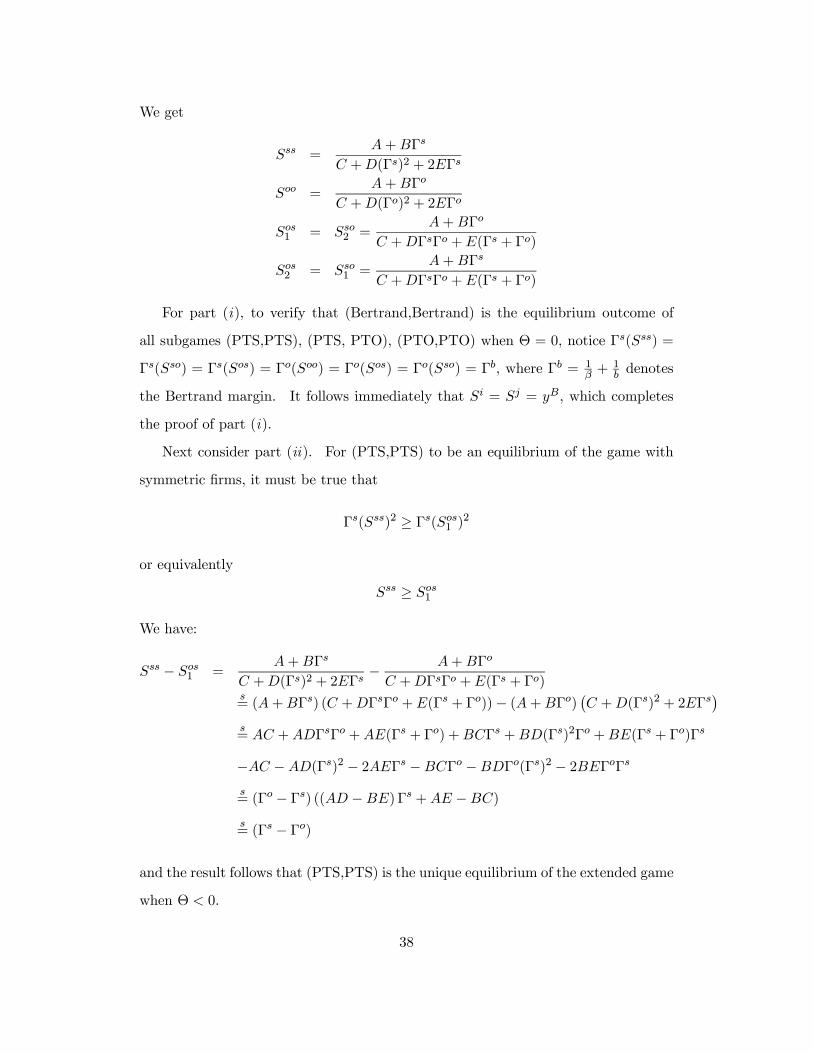
For part (i), to verify that (Bertrand,Bertrand) is the equilibrium outcome of

all subgames (PTS,PTS), (PTS, PTO), (PTO,PTO) when Θ = 0, notice Γs(Sss) =

Γs(Sso) = Γs(Sos) = Γo(Soo) = Γo(Sos) = Γo(Sso) = Γb, where Γb = 1β+ 1

bdenotes

the Bertrand margin. It follows immediately that Si = Sj = yB, which completes

the proof of part (i).

Next consider part (ii). For (PTS,PTS) to be an equilibrium of the game with

symmetric firms, it must be true that

Γs(Sss)2 ≥ Γs(Sos1 )2

or equivalently

Sss ≥ Sos1

We have:

Sss − Sos1 =A+BΓs

C +D(Γs)2 + 2EΓs− A+BΓo

C +DΓsΓo +E(Γs + Γo)s= (A+BΓs) (C +DΓsΓo +E(Γs + Γo))− (A+BΓo) ¡C +D(Γs)2 + 2EΓs¢s= AC +ADΓsΓo +AE(Γs + Γo) +BCΓs +BD(Γs)2Γo +BE(Γs + Γo)Γs

−AC −AD(Γs)2 − 2AEΓs −BCΓo −BDΓo(Γs)2 − 2BEΓoΓss= (Γo − Γs) ((AD −BE)Γs +AE −BC)s= (Γs − Γo)

and the result follows that (PTS,PTS) is the unique equilibrium of the extended game

when Θ < 0.

38

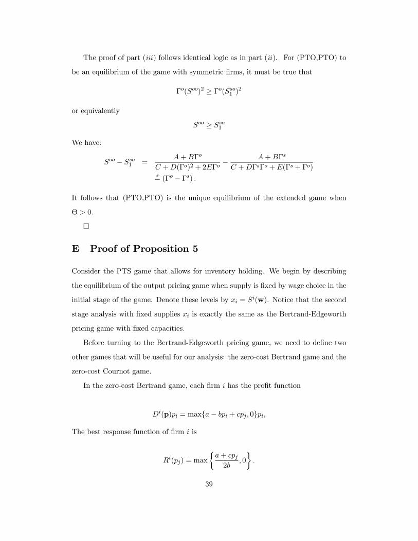
The proof of part (iii) follows identical logic as in part (ii). For (PTO,PTO) to

be an equilibrium of the game with symmetric firms, it must be true that

Γo(Soo)2 ≥ Γo(Sso1 )2

or equivalently

Soo ≥ Sso1We have:

Soo − Sso1 =A+BΓo

C +D(Γo)2 + 2EΓo− A+BΓs

C +DΓsΓo +E(Γs + Γo)s= (Γo − Γs) .

It follows that (PTO,PTO) is the unique equilibrium of the extended game when

Θ > 0.

¤

E Proof of Proposition 5

Consider the PTS game that allows for inventory holding. We begin by describing

the equilibrium of the output pricing game when supply is fixed by wage choice in the

initial stage of the game. Denote these levels by xi = Si(w). Notice that the second

stage analysis with fixed supplies xi is exactly the same as the Bertrand-Edgeworth

pricing game with fixed capacities.

Before turning to the Bertrand-Edgeworth pricing game, we need to define two

other games that will be useful for our analysis: the zero-cost Bertrand game and the

zero-cost Cournot game.

In the zero-cost Bertrand game, each firm i has the profit function

Di(p)pi = maxa− bpi + cpj , 0pi,

The best response function of firm i is

Ri(pj) = max

½a+ cpj

2b, 0

¾.

39

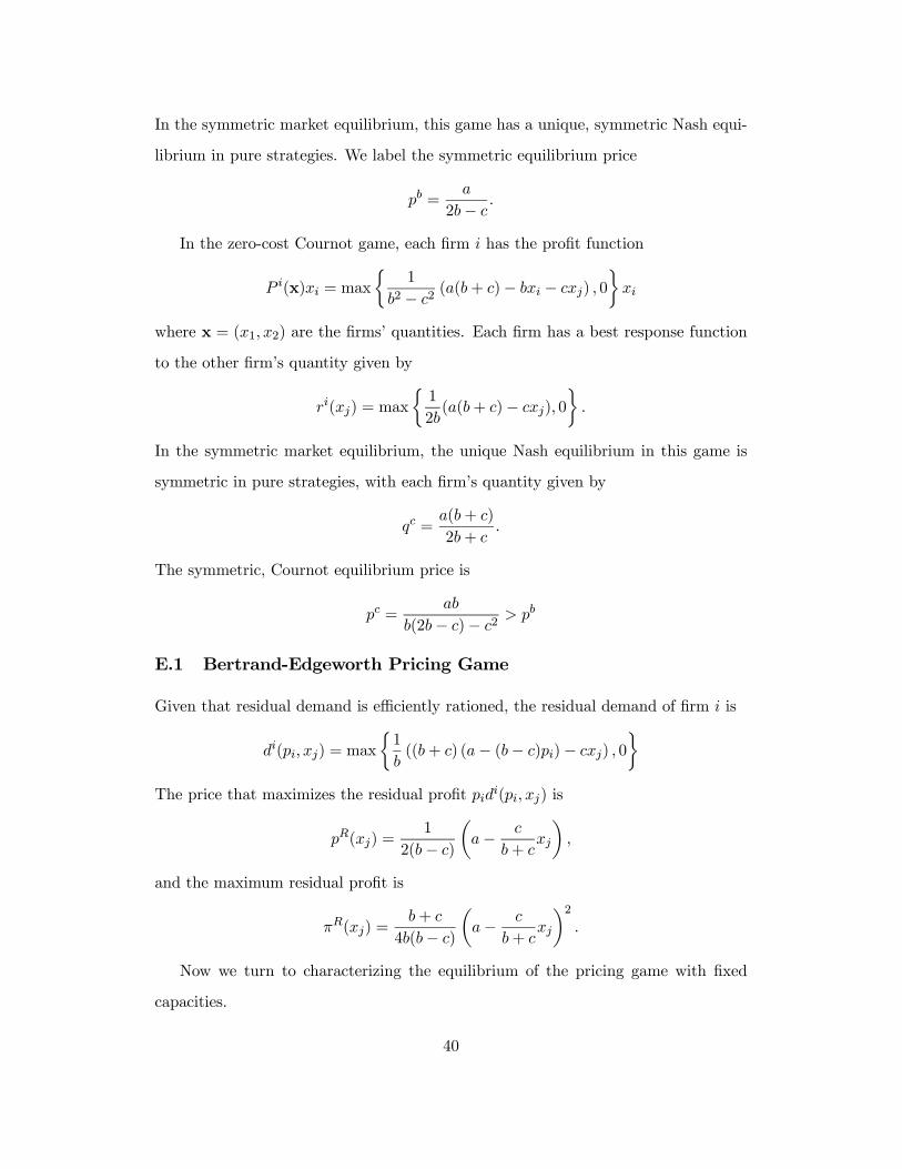
In the symmetric market equilibrium, this game has a unique, symmetric Nash equi-

librium in pure strategies. We label the symmetric equilibrium price

pb =a

2b− c .

In the zero-cost Cournot game, each firm i has the profit function

P i(x)xi = max

½1

b2 − c2 (a(b+ c)− bxi − cxj) , 0¾xi

where x = (x1, x2) are the firms’ quantities. Each firm has a best response function

to the other firm’s quantity given by

ri(xj) = max

½1

2b(a(b+ c)− cxj), 0

¾.

In the symmetric market equilibrium, the unique Nash equilibrium in this game is

symmetric in pure strategies, with each firm’s quantity given by

qc =a(b+ c)

2b+ c.

The symmetric, Cournot equilibrium price is

pc =ab

b(2b− c)− c2 > pb

E.1 Bertrand-Edgeworth Pricing Game

Given that residual demand is efficiently rationed, the residual demand of firm i is

di(pi, xj) = max

½1

b((b+ c) (a− (b− c)pi)− cxj) , 0

¾The price that maximizes the residual profit pid

i(pi, xj) is

pR(xj) =1

2(b− c)µa− c

b+ cxj

¶,

and the maximum residual profit is

πR(xj) =b+ c

4b(b− c)µa− c

b+ cxj

¶2.

Now we turn to characterizing the equilibrium of the pricing game with fixed

capacities.

40

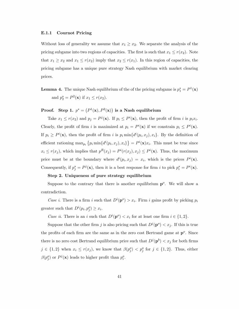
E.1.1 Cournot Pricing

Without loss of generality we assume that x1 ≥ x2. We separate the analysis of thepricing subgame into two regions of capacities. The first is such that x1 ≤ r(x2). Notethat x1 ≥ x2 and x1 ≤ r(x2) imply that x2 ≤ r(x1). In this region of capacities, thepricing subgame has a unique pure strategy Nash equilibrium with market clearing

prices.

Lemma 4. The unique Nash equilibrium of the of the pricing subgame is p∗1 = P1(x)

and p∗2 = P2(x) if x1 ≤ r(x2).

Proof. Step 1. p∗ =¡P 1(x), P 2(x)

¢is a Nash equilibrium

Take x1 ≤ r(x2) and pj = P j(x). If pi ≤ P i(x), then the profit of firm i is pixi.

Clearly, the profit of firm i is maximized at pi = P i(x) if we constrain pi ≤ P i(x).If pi ≥ P i(x), then the profit of firm i is pimindi(pi, xj), xi. By the definition ofefficient rationing maxpi

©pimindi(pi, xj), xi

ª= P i(x)xi. This must be true since

xi ≤ r(xj), which implies that pR(xj) = P i(r(xj), xj) ≤ P i(x). Thus, the maximumprice must be at the boundary where di(pi, xj) = xi, which is the prices P

i(x).

Consequently, if p∗j = Pj(x), then it is a best response for firm i to pick p∗i = P

i(x).

Step 2. Uniqueness of pure strategy equilibrium

Suppose to the contrary that there is another equilibrium po. We will show a

contradiction.

Case i. There is a firm i such that Di(po) > xi. Firm i gains profit by picking pi

greater such that Di(pi, poj) ≥ xi.

Case ii. There is an i such that Di(po) < xi for at least one firm i ∈ 1, 2.Suppose that the other firm j is also pricing such that Dj(po) < xj . If this is true

the profits of each firm are the same as in the zero cost Bertrand game at po. Since

there is no zero cost Bertrand equilibrium price such that Dj(pb) < xj for both firms

j ∈ 1, 2 when xi ≤ r(xj), we know that β(poj) < poj for j ∈ 1, 2. Thus, eitherβ(poj) or P

j(x) leads to higher profit than poi .

41

Suppose that the other firm j is pricing such that Dj(po) = xj . Then firm i is

operating on the residual demand, which is uniquely maximized at P i(x).

Case iii. Di(po) = xi for both firms i. Then at least one firm i must be playing

poi < P i(x). The other firm j’s best response is to maximize the residual demand

by which is uniquely done by picking P j(x). So poj = Pj(x). Consequently, firm i’s

unique best response to P i(x) is to maximize the residual profit with P i(x).

Step 3. Uniqueness of equilibrium

The argument is based on showing that if x1 ≤ r(x2), then the game has strategiccomplementaries and then appealing to Theorem 12 in Milgrom and Shannon (1994).

Adapting Milgrom and Shannon definition of a game with strategic complementarities

to our notation, we have: for every player i

1. Player i’s strategy space is a compact lattice;

2. Player i’s payoff function is upper semi-continuous in pi for pj fixed, and con-

tinuous in pj for fixed pi;

3. Player i’s payoff function is quasisupermodular in pi and satisfies the single

crossing property in (pi; pj).

The first two requirements are satisfied for the pricing game, since the interval

[0, P ] ⊂ R is a compact lattice and the profits are continuous functions in both

arguments. We are left to show that property three is satisfied.

The connection between monotonic nondecreasing best responses and the third

requirement for a game with strategic complementarities is based on the following

special case of Theorem 4 in Milgrom and Shannon (1994) modified to our notation.

[Milgrom and Shannon] Let π : [0, P ] × [0, P ] 7→ R. Then φ(ρ) is monotonic

nondecreasing in ρ if and only if π is quasisupermodular in p and satisfies the single

crossing property in (p; ρ).

Now we appeal to a special case of Milgrom and Shannon (1994), Theorem 12

modified to our notation:

42

[Milgrom and Shannon] In a game with strategic complementarities and a unique

pure strategy Nash equilibrium, the Nash equilibrium strategies are the unique serial

undominated strategies.

We will show that each firm’s best response is a nondecreasing function on [0, P ]

and then uniqueness follows from Fact 2. To do this, we show that the firms’ best

response correspondences are contained within monotonic nondecreasing correspon-

dence that have the unique pure strategy equilibrium¡P 1(x), P 2(x)

¢. Denote by

βC(p) the best response correspondence for the pricing subgame.

Define another correspondence

eβCj (p) = ½ [β(p), pR(xj)] p < pR(xj)

[pR(xj),β(p)] p ≥ pR(xj) .

eβCi is a monotonic nondecreasing correspondence on [0, P ] and is such that βCi (p) ∈eβCi (p) for all p ∈ [0, P ] for either firm i. Further, the unique pure strategy equilibriumof the game with best responses eβC is ¡P 1(x), P 2(x)¢.E.1.2 Mixed Pricing

In this section, we only prove what is necessary for the proof of our main proposition

about the PTS game with inventory-holding. We only need to consider x2 ≤ qc andwithout loss of generality x1 ≥ x2. We will use the following nomenclature throughoutthe proofs of this subsection: As denoted previously, the maximal residual profit is

πR(xj), we will refer to this as simply the residual profit. We denote the front-side

profit of firm i as the largest profit such that the firm j is best off taking the residual

demand.

Lemma 5. If x1 > r(x2), then π∗1 ≥ πR(x2)

Proof. By picking p1 = pR1 (x2) can always get at least the residual demand

d1(p1, x2) and hence at least the profit πR(x2).

Lemma 6. Firm 1’s front-side profit is less than its residual profit.

43

Proof. Take x1 ≥ x2 and r(x2) = x1 (note that it must be that x2 ≤ qc). This is theCournot pricing region characterized in Lemma E.1.1. In the Cournot pricing region

the front-side profit equals the residual profit, which equals the Cournot profit. Now

we will show an increase to x01 such that x01 > r(x2) decreases firm 1’s front-side profit

while not affecting firm its residual profit. First notice that the residual profit πR(x2)

is not affected by increasing x1. Now we show the front-side profit is decreasing in

x1. The front-side profit for firm 1 is bounded above by ρf1x1 where ρ

f1 = max0, pf1

and D2(ep2, pf1) = x2, where ep2 = πR(x1)/x2. We do not need to consider the case

that pf1 ≤ 0, since in that case the front-side profit is zero, which is clearly less than a

positive residual profit. Let us show that pf1x1 is decreasing in x1. Using our demand

specification and solving for pf1 we have

pf1 = −

(a− x2)c

+b

cep2.

We plug in with the functional forms and differentiate the front-side profit of firm 1

with regards to x1 to find

−(a− x2)c

+b

cx2πR(x1) +

b

cx2

∂πR(x1)

∂x1x1 < 0 (30)

The first term is negative, since x2 ≤ qc < a. Thus, if we can show that the sum of

the second two terms is negative than the whole expression must be negative as well.

Plugging in with the functional forms of πR(x1) and ∂πR(x1)/∂x1, (30) reduces to

the inequality

b

cx2

Ãb+ c

4b(b− c)µa− c

b+ cx1

¶2!<

b

cx2

µb+ c

2b(b− c)µa− c

b+ cx1

¶c

b+ cx1

¶a− c

b+ cx1 <

2c

b+ cx1

a(b+ c)

3c< x1.

The final inequality must be true because to be in x1 < r(x2), x1 > qc and qc >

a(b+ c)/3c.

Lemma 7. For x1 > r(x2), π∗2 > πR(x1)

44

Proof. Suppose to the contrary that firm 2 does not have an equilibrium profit

higher than πR(x1). Suppose that firm 2 plays ep2, then only if firm 1 plays p1 ≤ pf1it gets the front-side profit. We know that p

f1x1 < πR(x2) based on Lemma E.1.2.

Take ² > 0 and suppose firm 2 prices at ep2+², then firm 1 can price at most pf1+b²/cand get the front-side profit. For small enough ² > 0, p

f1x1 + b²x1/c < πR(x2). This

implies that there exists p02 > ep2 such that firm 1 will always prefer to maximize the

residual demand over undercutting and getting the front-side profit. Consequently,

firm 2 can guarantee itself a profit greater than maximizing the residual by picking

such a p02, since p02x2 > ep2x2 = πR(x1).

Lemma 8. For x1 > r(x2), π∗1 ≤ πR(x2).

Proof. Define pi as the least upper bound of the equilibrium best responses of any

firm i. The key aspect of this price pi is: Does firm i get residual for sure at pi? Note

that at least one firm i must get residual for sure at their pi. Denote by Pri(p) the

equilibrium probability that firm i does not get the residual demand at the price p.

The following cases can overlap.

Case i. At p1 firm 1 gets residual for sure. Consider the case that firm 1 has an

atom at p1 or firm 1 has best responses approaching p1. If firm 1 has an atom at

p1, then π∗1 = πR(x2) ≥ p1d1(p1, x2). If firm 1 has best responses approaching p1,

then and take any sequence of best responses pk1 ↑ p1 and limk→∞Pr1(pk1)pk1x1+(1−Pr1(p

k1))p

k1d1(pk1, x2) = p1d1(p1, x2) ≤ πR(x2).

Case ii. At p2 firm 2 gets residual for sure. Consider the case that firm 2 has

an atom at p1 or firm 2 has best responses approaching p2. We show that this

case cannot be. If firm 2 has an atom at p2, then π∗2 = πR(x2) ≥ p2d2(p2, x2),

which contradicts Lemma E.1.2. Take any sequence of best responses pk2 ↑ p2, thenlimk→∞Pr2(pk2)pk2x2 + (1 − Pr2(pk2))pk2d2(pk2, x1) = p2d

2(p2, x1) ≤ πc(x1). But,

again, based on Lemma E.1.2 we know that π∗2 > πR(x1), a contradiction.

We now turn to our primary results on inventory-holding behavior in the PTS

game.

45

E.2 PTS equilibrium with inventory holding

The PTS equilibrium wage bw is such thatSi(bw) ≤ qc (31)

Alternatively, we can define wc such that Si(wc) = qc and rewrite Condition 31

as

P ij (qc)S

jj (w

c) ≤ 1 + εSo (wc) (32)

We wish to show that if Condition E.2 holds, then the Nash equilibrium outcome in

the PTS game with a binding inventory constraint is a Nash equilibrium outcome of

the PTS game with inventory holding.

Proof. If Si(bw) ≤ qc, then only defections such that Si(w0i, bwj) > r(Sj( bwj , w0i))are potentially more profitable in the PTS game with inventory holding than the

PTS game. Any other defection results in exactly the same profit as the PTS game.

We first show that the profit of firm i is strictly concave over all w0i ≥ bwi suchthat Si(w0i, bwj) > r(Sj( bwj , w0i)) by showing using the fact that the profit is twicecontinuously differentiable.

∂2¡πR(S2)− w1S1

¢∂w21

=−γc2

2b(b2 − c2) − β < 0. (33)

Thus, the profit of firm 1 for all Si(w0i, bwj) > r(Sj( bwj , w0i)) is concave.At the boundary of Si(w0i, bwj) = r(Sj( bwj , w0i) is the only point where the profit

of firm i is not differentiable. Consequently, for such a defection to be profitable the

one at the boundary must be marginally better.

We know at w0i ≥ bwi such that Si(w0i, bwj) = r(Sj( bwj , w0i) that (based on bw as an

equilibrium of the PTS game)

P ij (Si, Sj)S

ji S

i − Si − w0iSii < 0 (34)

at such a w0i, it must be that Si = r(Sj). Thus, the inequality 34 implies that

P ij (r(Sj), Sj)r(Sj)S

ji − Si − wiSii < 0.

46

Based the strict concavity of the profit for all w0i ≥ bwi such that Si(w0i, bwj) >r(Sj( bwj , w0i))

P ij (r(Sj), Sj)r(Sj)S

ji − Si −wiSii

is non decreasing in w0i. Therefore, the expected profit is decreasing at all w0i such that

Si(w0i, bwj) > r(Sj( bwj , w0i)). This is a sufficient condition for no profitable defectionw0i from bw.F Proof of Proposition 6

Noting that Θ = ²s − ²d, the proof holds by inspection upon substitution by rear-ranging terms in equations (21) and (23). ¤

G Proof of Proposition 7

The proof is constructed by considering price movements from the Bertrand outcome

under PTS and PTO. In the case of an interior solution, the Bertrand outcome for

an agent facing a contract of the form in (24) is defined by the first-order condition

pi − wi − ti = Si(w)

Sii(w)− D

i(p)

Dii(p), i ∈ 1, 2.

In the PTS game, evaluating the agent’s input price condition (25) at the symmetric

Bertrand equilibrium position (wB, pB) gives

Πi,si (w

B, pB) ≡ SiDijS

ii

∆Θ

s= Θ. (35)

In the PTO game, evaluating the output price condition (26) at the symmetric

Bertrand equilibrium position (wB, pB) gives

Πi,oi (w

B, pB) ≡ DiDiiS

ij

ΣΘ

s= Θ. (36)

By Proposition 1, oligopoly profits rise with defections from the Bertrand equilibrium

(p0, w0) that involve p0 > pB and w0 < wB. Letting the adjusted margin per unit of

output of firm i be denoted bΓi = pi−wi−tiSi

, the equilibrium timing of the game is

determined by the adjusted margins according to Proposition 4. ¤

47