OLG Models - Home | Penn Economicseconomics.sas.upenn.edu/~jesusfv/lecture4_olg_models.pdfJesœs FernÆndez-Villaverde (PENN) OLG Models February 12, 2016 2 / 53 Overlapping Generations

OLG Models

Jesús Fernández-Villaverde

University of Pennsylvania

February 12, 2016

Jesús Fernández-Villaverde (PENN) OLG Models February 12, 2016 1 / 53

Overlapping Generations

The Overlapping Generations Model I

Besides the neoclassical growth model, the OLG model is the secondmajor workhorse of modern macroeconomics.

Pioneered by Allais (1947), Samuelson (1958), and Diamond (1965).

Important features of the model:

1 Competitive equilibria may be Pareto suboptimal.

2 Outside money may have positive value.

3 There may exist a continuum of equilibria.



Motivation I

Shortcoming of the infinitely lived agents model: individuals,apparently, do not live forever.

But:

1 Role of assumptions in economic theory. Friedman’s Essays on PositiveEconomics.

2 An altruistic bequest motive makes finitely lived individuals lived for afinite number of periods to maximize the utility of the entire dynasty.

More relevant motivation: we want models where agents undergo aninteresting life cycle with low-income youth, high income middle ages,and retirement where labor income drops to zero.



Motivation II

Why?

1 Integrate micro and macro data.

2 Analyze issues like social security, the effect of taxes on retirementdecisions, the distributive effects of taxes versus government deficits,the effects of life-cycle saving on capital accumulation, educationalpolicies, etc.

Final motivation: because of its interesting (some say, pathological)theoretical properties, it is also an area of intense study amongeconomic theorists.

How much should we believe those theoretical properties?

Role of quantitative OLG models with a large number of generations.


Setup

Basic Setup of the Model

Time is discrete, t = 1, 2, 3, . . . and the economy (but not its people)lives forever.

In each period there is a single, nonstorable consumption good.

In each time period a new generation (of measure 1) is born, whichwe index by its date of birth.

People live for two periods and then die.

Alternative: stochastic aging (Blanchard, 1985). We do not need tokeep track of age distributions.


Setup

Endowments and Consumption

(ett , ett+1): generation t’s endowment of the consumption good in the

first and second period of their live.

(c tt , ctt+1): consumption allocation of generation t.

In time t there are two generations alive:

1 One old generation t − 1 that has endowment et−1t and consumptionct−1t .

2 One young generation t that has endowment ett and consumption ctt .

In period 1 there is an initial old generation 0 that has endowment e01and consumes c01 .


Setup

Timing

generation\time 1 2 . . . t t + 10 (c01 , e

01 )

1 (c11 , e11 ) (c12 , e

12 )

.... . .

t − 1 (c t−1t , et−1t )t (c tt , e

tt ) (c tt+1, e

tt+1)

t + 1 (c t+1t+1 , et+1t+1 )


Setup

Double Infinities

There are both an infinite number of periods as well as well as aninfinite number of agents.

This “double infinity”has been cited to be the major source of thetheoretical peculiarities of the OLG model (prominently by Karl Shell).

For example, double infinity will be key for the failure of the firstfundamental welfare theorem to hold in the model.

Mechanism: value of aggregate endowment at equilibrium prices maynot be finite.


Setup

Outside and Inside Money

In some of our applications we will endow the initial generation withan amount of outside money m.

Outside money: money that is, on net, an asset of the privateeconomy. This includes fiat currency issued by the government.

Inside money (such as bank deposits) is both an asset as well as aliability of the private sector (in the case of deposits an asset of thedeposit holder, a liability to the bank).

If m ≥ 0, then m can be interpreted as fiat money.

If m < 0, one should envision the initial old people having borrowedfrom some institution (outside the model) and m is the amount to berepaid.


Setup

Preferences

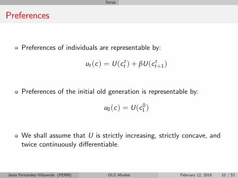
Preferences of individuals are representable by:

ut (c) = U(c tt ) + βU(c tt+1)

Preferences of the initial old generation is representable by:

u0(c) = U(c01 )

We shall assume that U is strictly increasing, strictly concave, andtwice continuously differentiable.


Setup

Allocations I

Definition

An allocation is a sequence c01 , {c tt , c tt+1}∞t=1.

Definition

An allocation is feasible if c t−1t , c tt ≥ 0 for all t ≥ 1 and

c t−1t + c tt = et−1t + ett for all t ≥ 1

Definition

An allocation is stationary if c tt−1, ctt ≥ 0 for all t ≥ 1 and

c t−1t = c tt = c for all t ≥ 1Jesús Fernández-Villaverde (PENN) OLG Models February 12, 2016 11 / 53

Setup

Allocations II

Definition

An allocation c01 , {(c tt , c tt+1)}∞t=1 is Pareto optimal if it is feasible and if

there is no other feasible allocation c10 , {(c tt , c tt+1)}∞t=1 such that:

ut (c tt , ctt+1) ≥ ut (c tt , c

tt+1) for all t ≥ 1

u0(c01 ) ≥ u0(c01 )

with strict inequality for at least one t ≥ 0.


Setup

Money as Numeraire

In the presence of money (m 6= 0), we will take money to be thenumeraire.

This is important since we can only normalize the price of onecommodity to 1.

With money, no further normalizations are admissible.

Let pt be the price of one unit of the consumption good at period t.


Markets Structure

Markets Structure

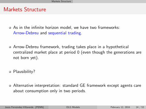
As in the infinite horizon model, we have two frameworks:Arrow-Debreu and sequential trading.

Arrow-Debreu framework, trading takes place in a hypotheticalcentralized market place at period 0 (even though the generations arenot born yet).

Plausibility?

Alternative interpretation: standard GE framework except agents careabout consumption only in two periods.


Markets Structure

Sequential Trading

Trade takes place sequentially in spot markets for consumption goodsthat open in each period.

In addition, there is an asset market through which individuals dotheir saving.

Let rt+1 be the interest rate from period t to period t + 1 and stt bethe savings of generation t from period t to period t + 1.

We will consider assets that cost one unit of consumption in period tand deliver 1+ rt+1 units tomorrow. Those assets are easier to handlethan zero-coupon bonds if the asset at hand is fiat money. However,both assets have identical implications.

We do not need a Ponzi condition.Jesús Fernández-Villaverde (PENN) OLG Models February 12, 2016 15 / 53

Markets Structure

Arrow-Debreu Equilibrium

Given m, an Arrow-Debreu equilibrium is an allocation c01 , {(c tt , c tt+1)}∞t=1

and prices {pt}∞t=1 such that

1 Given {pt}∞t=1, for each t ≥ 1, (c tt , c tt+1) solves:

max(c tt ,c

tt+1)≥0

ut (c tt , ctt+1)

s.t. ptc tt + pt+1ctt+1 ≤ ptett + pt+1ett+1

2 Given p1, c01 solves:

maxc01u0(c01 )

s.t. p1c01 ≤ p1e01 +m

3 For all t ≥ 1 (resource balance or goods market clearing):



Markets Structure

Sequential Markets Equilibrium

Given m, a sequential markets equilibrium is an allocation c01 ,{(c tt , c tt+1, stt )}∞

t=1 and interest rates {rt}∞t=1 such that:

1 Given {rt}∞t=1 for each t ≥ 1, (c tt , c tt+1, stt ) solves:

max(c tt ,c

tt+1)≥0,s tt

ut (c tt , ctt+1)

s.t. c tt + stt ≤ ett

c tt+1 ≤ ett+1 + (1+ rt+1)stt2 Given r1, c01 solves:

maxc01u0(c01 )

s.t. c01 ≤ e01 + (1+ r1)m3 For all t ≥ 1 (resource balance or goods market clearing):



Markets Structure

Market Clearing Condition for the Asset Market I

Given that the period utility function U is strictly increasing, thebudget constraints hold with equality.

Summing the budget constraints of agents:

c tt+1 + ct+1t+1 + s

t+1t+1 = e

tt+1 + e

t+1t+1 + (1+ rt+1)s

tt

By resource balance:

st+1t+1 = (1+ rt+1)stt

Doing the same manipulations for generation 0 and 1:

s11 = (1+ r1)m


Markets Structure

Market Clearing Condition for the Asset Market II

By repeated substitution:

stt = Πtτ=1(1+ rτ)m

The amount of saving (in terms of the period t consumption good)has to equal the value of the outside supply of assets, Πt

τ=1(1+ rτ)m.

Interpretation.

This condition should appear in the definition of equilibrium. ByWalras’law however, either the asset market or the good marketequilibrium condition is redundant.


Markets Structure

Equivalence between Equilibria

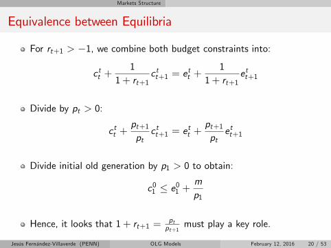
For rt+1 > −1, we combine both budget constraints into:

c tt +1

1+ rt+1c tt+1 = e

tt +

11+ rt+1

ett+1

Divide by pt > 0:

c tt +pt+1pt

c tt+1 = ett +

pt+1pt

ett+1

Divide initial old generation by p1 > 0 to obtain:

c01 ≤ e01 +mp1

Hence, it looks that 1+ rt+1 =ptpt+1

must play a key role.


Markets Structure

Equivalence Proposition

Given equilibrium Arrow-Debreu prices {pt}∞t=1, define interest rates:

1+ rt+1 =ptpt+1

1+ r1 =1p1

These interest rates induce a sequential markets equilibrium with thesame allocation than the Arrow-Debreu equilibrium.Conversely, given equilibrium sequential markets interest rates interestrates {rt}∞

t=1, define Arrow-Debreu prices by

p1 =1

1+ r1

pt+1 =pt

1+ rt+1These prices induce allocations that are equivalent to the sequentialmarkets equilibrium.


Markets Structure

Return on Money

From the equivalence, the return on the asset equals:

1+ rt+1 =ptpt+1

=1

1+ πt+1

(1+ rt+1)(1+ πt+1) = 1

rt+1 ≈ −πt+1

where πt+1 is the inflation rate from period t to t + 1.

The real return on money equals the negative of the inflation rate.


Markets Structure

More on the Equivalence I

Using:

p1 =1

1+ r1

pt+1 =pt

1+ rt+1

with repeated substitution delivers:

pt =1

Πtτ=1(1+ rτ)

⇒ Πtτ=1(1+ rτ) =

1pt

Interpretation.


Markets Structure

More on the Equivalence II

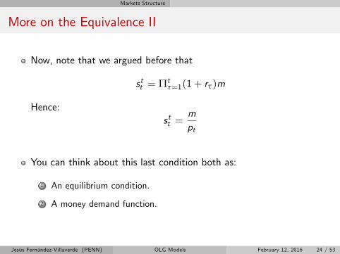
Now, note that we argued before that

stt = Πtτ=1(1+ rτ)m

Hence:stt =

mpt

You can think about this last condition both as:

1 An equilibrium condition.

2 A money demand function.


Offer Curves

Offer Curves

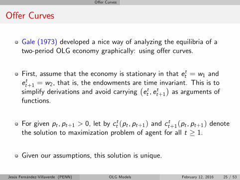
Gale (1973) developed a nice way of analyzing the equilibria of atwo-period OLG economy graphically: using offer curves.

First, assume that the economy is stationary in that ett = w1 andett+1 = w2, that is, the endowments are time invariant. This is tosimplify derivations and avoid carrying

(ett , e

tt+1

)as arguments of

functions.

For given pt , pt+1 > 0, let by c tt (pt , pt+1) and ctt+1(pt , pt+1) denote

the solution to maximization problem of agent for all t ≥ 1.

Given our assumptions, this solution is unique.


Offer Curves

Excess Demand Functions

Define the excess demand functions:

y(pt , pt+1) = c tt (pt , pt+1)− w1z(pt , pt+1) = c tt+1(pt , pt+1)− w2

These functions summarize, for given prices, consumer optimization.y and z only depend on pt+1

pt, but not on pt and pt+1 separately (the

excess demand functions are homogeneous of degree zero in prices).Varying pt+1

ptbetween 0 and ∞ (not inclusive), we obtain the offer

curve: a locus of optimal excess demands in (y , z) space:

(y , f (y))

f can be a multi-valued correspondence.A point on the offer curve is an optimal excess demand function forsome pt+1

pt∈ (0,∞).


Offer Curves

z(p ,p )t t+1

y(p ,p )t t+1

Offer Curve z(y)

w2

w1


Offer Curves

More on Offer Curves I

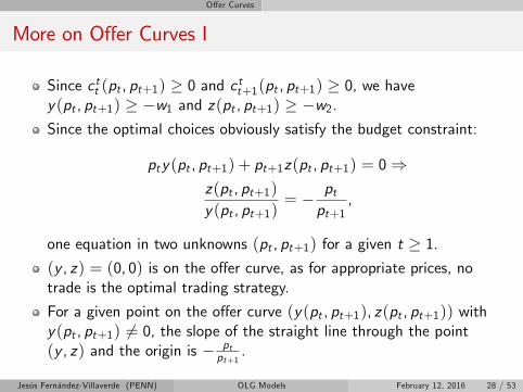
Since c tt (pt , pt+1) ≥ 0 and c tt+1(pt , pt+1) ≥ 0, we havey(pt , pt+1) ≥ −w1 and z(pt , pt+1) ≥ −w2.Since the optimal choices obviously satisfy the budget constraint:

pty(pt , pt+1) + pt+1z(pt , pt+1) = 0⇒z(pt , pt+1)y(pt , pt+1)

= − ptpt+1

,

one equation in two unknowns (pt , pt+1) for a given t ≥ 1.(y , z) = (0, 0) is on the offer curve, as for appropriate prices, notrade is the optimal trading strategy.

For a given point on the offer curve (y(pt , pt+1), z(pt , pt+1)) withy(pt , pt+1) 6= 0, the slope of the straight line through the point(y , z) and the origin is − pt

pt+1.


Offer Curves

More on Offer Curves II

We can express goods market clearing in terms of excess demandfunctions as

y(pt , pt+1) + z(pt−1, pt ) = 0

Also, for the initial old generation the excess demand function is givenby

z0(p1,m) =mp1

so that the goods market equilibrium condition for the first periodreads as

y(p1, p2) + z0(p1,m) = 0


Offer Curves

More on Offer Curves III

Finally, note that we have:

stt = −y(pt , pt+1) =mpt

andz(pt , pt+1) =

mpt+1

These conditions highlight the role of money as a mechanism forintertemporal trade.


Offer Curves

More on Offer Curves IV

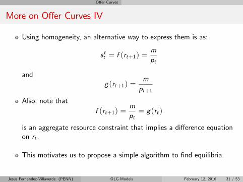
Using homogeneity, an alternative way to express them is as:

stt = f (rt+1) =mpt

andg(rt+1) =

mpt+1

Also, note thatf (rt+1) =

mpt= g(rt )

is an aggregate resource constraint that implies a difference equationon rt .

This motivates us to propose a simple algorithm to find equilibria.


Offer Curves

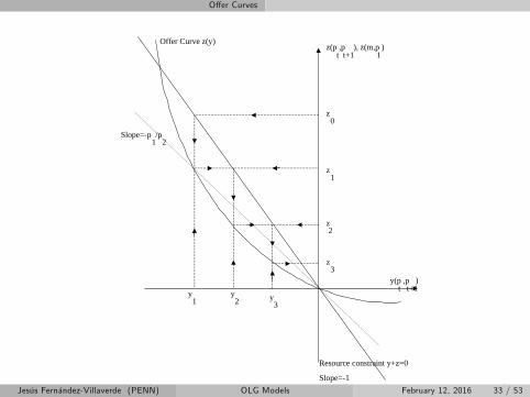
Algorithm to Find Equilibria

1 Pick an initial price p1 (this is NOT a normalization since p1determines the real value of money m

p1the initial old generation is

endowed with; we have already normalized the price of money).Hence, we know z0(p1,m). This determines y(p1, p2).

2 From the offer curve, we determine z(p1, p2) ∈ f (y(p1, p2)). Notethat if f is a correspondence then there are multiple choices for z .

3 Once we know z(p1, p2), we can find y(p2, p3) and so forth. In thisway we determine the entire equilibrium consumption allocation:

c01 = z0(p1,m) + w2c tt = y(pt , pt+1) + w1

c tt+1 = z(pt , pt+1) + w2

4 Equilibrium prices can then be found, given p1.


Offer Curves

z(p ,p ), z(m,p )t t+1 1

y(p ,p )t t+1

Offer Curve z(y)

z0

z1

z2

z3

y1

y2 y

3

Slope=p /p1 2

Resource constraint y+z=0

Slope=1Jesús Fernández-Villaverde (PENN) OLG Models February 12, 2016 33 / 53

Offer Curves

Remarks

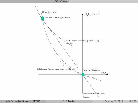
Any initial p1 that induces sequences c01 , {(c tt , c tt+1), pt}∞t=1 such that

the consumption sequence satisfies c t−1t , c tt ≥ 0 is an equilibrium forgiven money stock.

This already indicates the possibility of a lot of equilibria for thismodel.

In general, the price ratio supporting the autarkic equilibrium satisfies:

ptpt+1

=U ′(ett )

βU ′(ett+1)=

U ′(w1)βU ′(w2)

and this ratio represents the slope of the offer curve at the origin.


Offer Curves

z(p ,p ), z(m,p )t t+1 1

y(p ,p )t t+1

Offer Curve z(y)


Slope=1

Autarkic Allocation

Paretodominating allocation

Indifference Curve through dominatingallocation

Indifference Curve through autarkic allocation


Ineffi ciencies

Samuelson versus Classical Case

Define the autarkic interest rate as:

1+ r =U ′(w1)

βU ′(w2)

Gale (1973):

1 Samuelson case: r < 0.

2 Classical case: r ≥ 0.


Ineffi ciencies

Ineffi cient Equilibria I

Competitive equilibria in OLG models may be not be Pareto optimal.

Suffi cient Condition

If ∑∞t=1 pt < ∞, then the competitive equilibrium allocation for any pure

exchange OLG economy is Pareto-effi cient.

If, however, the value of the aggregate endowment is infinite (at theequilibrium prices), then the competitive equilibrium MAY not bePareto optimal.

Ineffi ciency is therefore associated with low (negative) interest rates.


Ineffi ciencies

Ineffi cient Equilibria II

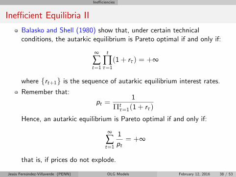
Balasko and Shell (1980) show that, under certain technicalconditions, the autarkic equilibrium is Pareto optimal if and only if:

∞

∑t=1

t

∏τ=1(1+ rτ) = +∞

where {rt+1} is the sequence of autarkic equilibrium interest rates.

Remember that:pt =

1Πt

τ=1(1+ rτ)

Hence, an autarkic equilibrium is Pareto optimal if and only if:

∞

∑t=1

1pt= +∞

that is, if prices do not explode.


Ineffi ciencies

Intuition I

Take the autarkic allocation and try to construct a Paretoimprovement.

In particular, give additional δ0 > 0 units of consumption to theinitial old generation. This obviously improves this generation’s life.

From resource feasibility this requires taking away δ0 from generation1 in their first period of life.

To make them not worse off, they have to receive δ1 in additionalconsumption in their second period of life, with δ1 satisfying

δ0U ′(e11 ) = δ1βU ′(e12 )

or

δ1 = δ0U ′(e11 )

βU ′(e12 )= δ0(1+ r2)−1 > 0


Ineffi ciencies

Intuition II

In general, the required transfers in the second period of generationt’s life to compensate for the reduction of first period consumption:

δt = δ0t

∏τ=1(1+ rτ+1)−1

Such a scheme does not work if the economy ends at fine time Tsince the last generation (that lives only through youth) is worse off.

But as our economy extends forever, such an intergenerationaltransfer scheme is feasible provided that the δt do not grow too fast,that is, if interest rates are suffi ciently small.

But if such a transfer scheme is feasible, then we found a Paretoimprovement over the original autarkic allocation, and hence theautarkic equilibrium allocation is not Pareto effi cient.


More on Money

Positive Valuation of Outside Money

Second main result of OLG models: outside money may have positivevalue.

Money in this equilibrium is a bubble:

1 The fundamental value of an assets is the value of its dividends,evaluated at the equilibrium Arrow-Debreu prices.

2 An asset has a bubble if its price does not equal its fundamental value.

3 Since money does not pay dividends, its fundamental value is zero andthe fact that it is valued positively in equilibrium makes it a bubble.


More on Money

Intuition I

The currently young generation transfer some of their endowment tothe old people for pieces of paper because they expect (correctly so,in equilibrium) to exchange these pieces of paper against consumptiongoods when they are old.

Hence, we achieve an intertemporal allocation of consumption goodsthat dominates the autarkic allocation.

Without the outside asset, again, this economy can do nothing elsebut remain in the possibly dismal state of autarky.


More on Money

Intuition II

This is why the social contrivance of money is so useful in thiseconomy.

As we will see later, other institutions (for example a pay-as-you-gosocial security system or a gift-giving mechanism) may achieve thesame as money.

Relation with search models of money.

More general point: money is memory (Kocherlakota, 1998).


More on Money

Comparison with Exchange Economies

TheoremIn pure exchange economies with a finite number of infinitely lived agents,there cannot be an equilibrium in which outside money is valued.

Proof

Suppose, that there is an equilibrium {(c it )i∈I }∞t=1, {pt}∞

t=1 for initialendowments of outside money (mi )i∈I such that ∑i∈I m

i 6= 0. By localnonsatiation:

∞

∑t=1pt c it = ∑

t=1pte it +m

i < ∞

Summing over all individuals i ∈ I yields ∑∞t=1 pt ∑i∈I

(c it − e it

)= ∑i∈I m

i .But resource feasibility requires ∑i∈I

(c it − e it

)= 0 for all t ≥ 1 and hence

∑i∈I mi = 0, a contradiction.


More on Money

Deficit Finance I

Presence of money allows to think about government financing:issuing or retiring currency. Hence, we will index mt .

Imagine government consumption g .

Thrown into the sea (or enters separably in the utility function).

Lump sum taxes on each generation τ1 and τ2.

Constant endowment (as in the offer curves section).

Then:mt −mt−1 = pt (g − τ1 − τ2) = ptd


More on Money

Deficit Finance II

Now, remember that f (rt+1) = mtpt.

Hence:

f (rt+1)︸︷︷︸Young Saving

=mt−1pt︸︷︷︸

Old Dissaving

+mt −mt−1

pt︸︷︷︸Government Dissaving

=mt−1pt

+ d

=mt−1pt−1

pt−1pt

+ d

= f (rt ) (1+ rt ) + d

with initial equationf (r1) =

m0p1+ d


More on Money

Deficit Finance III

Since endowments are constant, we can solve the difference equationby “guess-and-verify” a constant interest rate:

f (r) = f (r) (1+ r) + d ⇒rf (r) = d

andf (r) =

m0p1+ d

Since r is a tax on real balances, rf (r) is a Laffer curve.

Multiple equilibria:

1 Stationary and non-starionary (continuum).2 Pareto-ranked.

More general property: existence of interesting equilibria.


Interesting Equilibria

Continuum of Equilibria I

Third major difference: the possibility of a whole continuum ofequilibria in OLG models.

General proof is complicated.

We can build non-stationary equilibria that in the limit converge tothe same allocation (autarky), they differ in the sense that at anyfinite t, the consumption allocations and price ratios (and levels) differacross equilibria. These equilibria are arbitrarily close to each other.

This is again in stark contrast to standard Arrow-Debreu economieswhere, generically, the set of equilibria is finite and all equilibria arelocally unique.

Generically: for almost all endowments, that is, the set of possiblevalues for the endowments for which this statement does not hold isof measure zero.



Continuum of Equilibria II

Local uniqueness: for every equilibrium price vector there exists ε suchthat any ε-neighborhood of the price vector does not contain anotherequilibrium price vector, apart from the trivial ones involving adifferent normalization (Debreu, 1970).

If we are in the Samuelson case r < 0, then (and only then) all theseequilibria are Pareto-ranked.

If we introduce a productive asset with positive dividends and nomoney, there exists a unique equilibrium, which is Pareto optimal.

It is not the existence of a long-lived outside asset that is responsiblefor the existence of a continuum of equilibria.

If we introduce a Lucas tree with negative dividends (the initial oldgeneration is an eternal slave, say, of the government and has to comeup with d in every period to be used for government consumption),then the existence of the whole continuum of equilibria is restored.



Endogenous Cycles

The equilibria in OLG economies need not be monotonic.

Instead, equilibria with cycles are possible.

Take an offer curve that is backward bending.

After period t = 2 the economy repeats the cycle from the first twoperiods.

In addition, we will have sunspots.



z(p ,p ), z(m,p )t t+1 1

y(p ,p )t t+1

Offer Curve z(y)

z1

z0

y2

y1


Slope=1

p /p2 3

p /p1 2



Equilibrium

The equilibrium allocation is of the form:

c t−1t =

{col = z0 − w2 for t oddcoh = z1 − w2 for t even

c tt =

{cyl = y1 − w1 for t oddcyh = y2 − w1 for t even

with col < coh, cyl < cyh.

Prices satisfy:

ptpt+1

=

{αh for t oddαl for t even

πt+1 = −rt+1 ={

πl < 0 for t oddπh > 0 for t even



Remarks

Note that these cycles are purely endogenous in the sense that theenvironment is completely stationary: nothing distinguishes odd andeven periods.

Also note that it is not particularly diffi cult to construct cycles oflength bigger than 2 periods.

We can also build chaotic economies.

Some economists have taken this feature of OLG models to be thebasis of a theory of endogenous business cycles (see, for example,Grandmont, 1985).


Documents

OLG Models - Home | Penn Economicseconomics.sas.upenn.edu/~jesusfv/lecture4_olg_models.pdfJesœs FernÆndez-Villaverde (PENN) OLG Models February 12, 2016 2 / 53 Overlapping Generations