Oil price shocks and fiscal policy management ... · Since 1970s there have been five main negative oil shocks. The first was from 1973 to 1974 whose fluctuation was as a result of

Special Issue: Development and Sustainability in Africa – Part 1

International Journal of Development and Sustainability

Online ISSN: 2186-8662 – www.isdsnet.com/ijds

Volume 1 Number 3 (2012): Pages 1121-1139

ISDS Article ID: IJDS12082301

Oil price shocks and fiscal policy management: Implications for Nigerian economic planning (1980-2009)

Adeleke Gabriel Aremo 1*, Monica Adele Orisadare 1, C. Moses Ekperiware 2

1 Obafemi Awolowo University,Ile-Ife, Nigeria 2 National Centre for Technology Management (NACETEM), Obafemi Awolowo University, Ile-Ife, Nigeria

Abstract

High Oil price fluctuations have been a common feature in Nigeria and these have considerably constituted a major

source of fiscal policy disturbance to the Nigerian economy as well as the economies of other oil producing countries

of the world. The over-reliance on oil production for income generation combined with local undiversified revenue

and export bases is an issue for concern. This has policy implications for economic policy and in particular fiscal

policy management. The motivation for this study is to examine the effect of oil price shock on fiscal policy in the

country. Using structural vector autoregression (SVAR) methodology, the effects of crude oil price fluctuations on

two major key fiscal policy variables (government expenditure (GEXP) and government revenue (GREV)), money

supply (MS2) and GDP were examined. The results showed that oil prices have significant effect on fiscal policy in

Nigeria within the study period of 1980:1 to 2009:4. The study also revealed that oil price shock affects GREV and

GDP first before reflecting on fiscal expenditure. The study suggests strongly that diversification of the economy is

necessary in order to minimize the consequences of oil price fluctuations on government revenue, by implication

government expenditure planning in the country.

Keywords: Oil price shock, Fiscal policy, Nigerian economic planning

Copyright © 2012 by the Author(s) – Published by ISDS LLC, Japan

International Society for Development and Sustainability (ISDS)

Cite this paper as: Aremo, A.G., Orisadare, M.A. and Ekperiware, C.M. (2012), “Oil price shocks and

fiscal policy management: Implications for Nigerian economic planning (1980-2009)”, International

Journal of Development and Sustainability, Vol. 1 No. 3, pp. 1121-1139.

* Corresponding author. E-mail address: [email protected]

International Journal of Development and Sustainability Vol.1 No.3 (2012): 1121-1139

1122 ISDS www.isdsnet.com

1. Introduction

The huge natural endowment and location of Nigerian outside the unstable Persian Gulf support the

speculation that her global demands for oil and gas would remain high many years to come. While this is

good for the country, its major problem has being managing the natural resources to reflect in sectors of the

economy. This is because Nigeria risk repeating patterns of weak economic governance and volatile spending

unless its policies feature certain safeguards to cushion the effects of shock from the country’s main revenue

source.

The problems created by abundant mineral wealth are not unique to Nigeria. The oil price shock and the

impending uncertainties could cause inaccurate state revenue forecast and is a major concern of the oil-

exporting countries (e.g Saudi Arabia, Libya, Kuwait etc), which depend heavily on oil revenue for their

public projects. Auty (2001) observed that oil exporting countries tend to suffer from a cluster of economic

and political ailments. Sachs and Warner (1997, 2001) and Manzano and Rigobon (2001) see it as an

atypically slow economic growth unusually with high rate corruption. While Leite and Weidemann (1999)

and Gylfason (2001) asserted that oil producing governments are correlated with abnormally low rates of

democratization.

The problem was so severe between 1970 and 1980 that the Nigerian government has to embark on

structural adjustment program (SAP) even before oil prices began to fall. This resulted in huge government

expenditure over revenue which led to the increase of Nigerian external borrowing. The external and

internal imbalances disrupted the nation developmental plans over the years. Economic planning and

budgeting in Nigeria are now benchmarked on oil price fluctuations to be able to achieve government

policies. The volatility and uncertainty that now plague oil earnings have resulted in unpredictable

investment climate in the country because nobody knows when the next shock will take place. This is likely

because they cannot predict the direction of the next shock or which sector will be favored. This uncertainty

has even affected the risk that investors face in non-oil activities. World Bank report has also confirmed that

oil price shocks are one of the main factors limiting private investment in developing economies. "With

high oil prices and high revenues, project selection criteria became very lax. Belief in the oil boom

encouraged Nigeria to finance large public expenditure programs. But the qualities of most of the

investments were so poor that many investments did not pay for themselves. Some projects that might have

become viable had oil prices remained high turned non-viable when oil prices fell. For political reasons,

however, the projects were not shut down" (Montenegro, 1994) e.g. the Ajaokuta iron and steel project.

One of the issues with oil price shock is that it leads to Capital flight, which is the response of investors to

fear of likely unsustainable budget deficits will bring inflation and higher future taxes. Also, appropriating

windfalls during booms and to avoid losses during the downturn has often been an unproductive political

struggle among the economic players in Nigeria. Husain et al. (2008) observed some countries in which the

oil sector is large in relation to the economy, oil price changes affect the economic cycle only through fiscal

policy.

Studies have revealed that unstable fiscal policy stance, reflecting changes in oil price fiscal revenue have

worsen output cycles in oil endowed countries (Balassone and Kumar, 2007; Kumah and Matovu, 2005;


ISDS www.isdsnet.com 1123

Baldini, 2005). However, some studies from Nigeria did not find significant impact of oil price shock on

variables like; money supply, price level, and output and government expenditure (Olusegun, 2008;

Christopher and Benedikt, 2006; and Philip and Akintoye, 2006).

Merlevede et al. (2009) observed a downward vulnerable oil price shocks in Russian economy but

concluded that the stabilisation brought by the Oil Stabilisation Fund and The fiscal policies of the Putin

administration reduced the economic effects of oil price shocks in the Russian economy. Hence, deliberate

management of fiscal policies of oil endowed nations are crucial to mitigate the effects of oil price shocks to

the lowest ebb. However, it was observed oil endowed nations suffers economic fluctuations because of oil

price shock, especially due to the rate of dependency which is not supposed to be as they case observed in

Nigeria. Nigeria’s economy vulnerability to fluctuations in international oil price shocks has been affirmed by

Omisakin et al. (2009).

Most of the empirical studies that have been carried out in the literature have centered on importing

economies located in the developed world. Few studies are available on the effect of oil price shocks on the

fiscal policy management in the world oil exporting countries, particularly in Nigeria. The focus of the few

existing studies has been broadly based on assessing the effect of oil price shocks on the broad

macroeconomic variables (see the work of Olomola and Adejumo, 2006). The present study is different from

the existing ones as it focuses on specific economic policy – fiscal policy – which makes it a candidate for

detailed analysis. Also, most of the studies in this area terminated in 2006.; thus, this present study will not

only add to the extant literatures, but will provide updated knowledge on the efffect of oil price shocks on

fiscal policy episodes experienced in Nigeria. In addition, Structural Vector Autoregession (SVAR) technique

has been applied to extended time series data to examine the link between the changes in oil price,

government revenue and government expenditures. Against this background therefore, the specific

objectives of the study are to analyse the impacts of oil price shock on fiscal policy in Nigeria in the past 40

years and also assess the magnitude of such impacts.

This paper is structured in five sections. Besides the introductory section, the historical trend in oil price

and fiscal policy is presented in section 2. Section 3 focuses on the theoretical framework and literature

review. Section 4 covers model specification. Section 5 focuses on data analysis and discussion of result while

section 6 concludes the paper with policy implications.

2. Historical trend in oil price and fiscal policy

With the discovery of oil in 1956 and its exportation in 1958, Nigeria ranked 4th amongst OPEC producing

countries in 2007. Oil has since been the dominant factor in income generation in Nigeria since the past 50

years, accounting for one third of the GDP, more than 90 percent of the exports and 80% of government

revenues (Ogbonna and Appah, 2012 and Charles et al., 2009).

The fact that Nigeria is particularly vulnerable to oil shocks is a phenomenon which has unfortunately

made the country severely affected by the fluctuations of the international oil prices, a situation which has in

turn contributed greatly to fluctuations in government budget revenue and expenditure. On the contrary, the



developed nations really more on the real sector activities in generating their resources like; income tax and

often supplemented by borrowing from the public. In Nigeria, the oil revenue is the key source of

government revenue that directs the course of spending. So, instability in price of oil in the international

market would lead to unstable implementation of government projects accurately been financed with oil

money.

According to the UN, (2005) a major source of oil price volatility in the markets today can be explained by

the differences in information assymmetry among market participants. Other factors driving oil price

fluctuations include: crude oil inventories, existence of futures exchanges in the market, disagreements on

production quotas and members' mistrust have added to uncertainty and fuelled volatility, weather, short-

term political developments, transportation problems (shipping, pipeline etc.), economic growth, problems

along the production- consumption chain, and even comments by OPEC members and leaders of oil-

producing countries, as well as demonstrations as witnessed in Nigeria, Venezuela and elsewhere. At times

alarmist price forecasts also contribute to the public's uncertainty regarding future oil prices.

Since 1970s there have been five main negative oil shocks. The first was from 1973 to 1974 whose

fluctuation was as a result of the OPEC oil embargo then. Followed by the period 1978 to 1979, when OPEC

reduced Nigeria’s production quota in her cartel policy to reduce world oil production which increased world

oil price including the Iran-Iraq war in early 1980s which escalated the price further. However, the Saudi

Arabia increased crude oil production decreased oil price in the mid-1980s. Between 1990 and 1991, Iraqi

invasion of Kuwait leads to another price shock. Also, the period 1999-2000, observed OPEC limiting its

world production of oil leading to another price shock. The last oil price shock took off in 2003 and rose

continuously to reach a peak of $137/pbl in July 2008 but after that a declining trend has set in. Oil price

shocks during the period mentioned were an important source of economic fluctuations. For example, oil

shocks of mid and late 1970s was followed by low growth, high unemployment, high government spending

and inflation in Nigeria. Illustration of the trend of some macroeconomic variables is worthwhile.

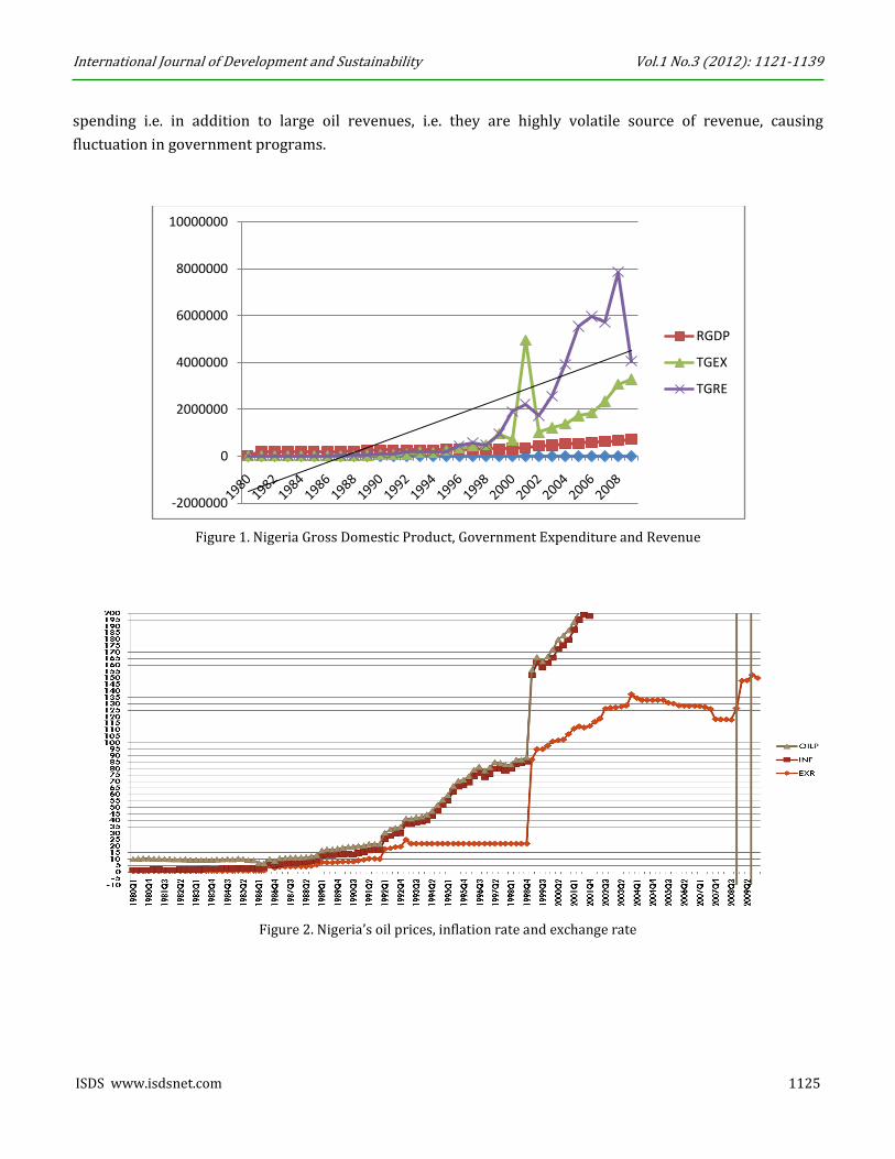
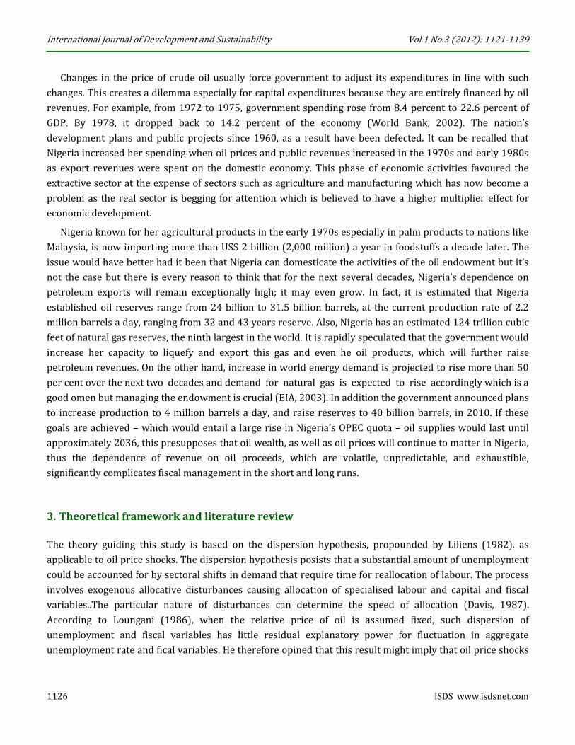
Figures 1 and 2 show a clear positive trend in government expenditure and inflation rate, such that

periods of increased government expenditure corresponds to periods of rising inflation rate. The relationship

between inflation rate and oil prices is closely linked and positive from the late 1990s up till the end of the

study period. Higher government spending also corresponds to rising inflation rate, suggesting the negative

impact of government spending on the inflation rate. Also, the gap that exists between government revenue

and government expenditure largely suggests that government revenues are not adequately channeled to

public expenditure that could substantially improve the general weal of the people.

Government spending is categorized into recurrent and capital expenditures. The main source of revenue

for government is oil exports revenue, which it has no control of because crude oil is a publicly traded

commodity by OPEC and its price is determined by the forces of demand and supply worldwide. When the

government is faced with abrupt fluctuations in oil prices, its forecast of recurrent as well as capital

expenditures becomes complicated and often imprecise. The fact that oil revenue is a major source of income

for the government of Nigeria implies that oil price shock imposes serious disruptive effects on government



spending i.e. in addition to large oil revenues, i.e. they are highly volatile source of revenue, causing

fluctuation in government programs.

Figure 1. Nigeria Gross Domestic Product, Government Expenditure and Revenue

Figure 2. Nigeria’s oil prices, inflation rate and exchange rate

-2000000

0

2000000

4000000

6000000

8000000

10000000

RGDP

TGEX

TGRE



Changes in the price of crude oil usually force government to adjust its expenditures in line with such

changes. This creates a dilemma especially for capital expenditures because they are entirely financed by oil

revenues, For example, from 1972 to 1975, government spending rose from 8.4 percent to 22.6 percent of

GDP. By 1978, it dropped back to 14.2 percent of the economy (World Bank, 2002). The nation’s

development plans and public projects since 1960, as a result have been defected. It can be recalled that

Nigeria increased her spending when oil prices and public revenues increased in the 1970s and early 1980s

as export revenues were spent on the domestic economy. This phase of economic activities favoured the

extractive sector at the expense of sectors such as agriculture and manufacturing which has now become a

problem as the real sector is begging for attention which is believed to have a higher multiplier effect for

economic development.

Nigeria known for her agricultural products in the early 1970s especially in palm products to nations like

Malaysia, is now importing more than US$ 2 billion (2,000 million) a year in foodstuffs a decade later. The

issue would have better had it been that Nigeria can domesticate the activities of the oil endowment but it’s

not the case but there is every reason to think that for the next several decades, Nigeria’s dependence on

petroleum exports will remain exceptionally high; it may even grow. In fact, it is estimated that Nigeria

established oil reserves range from 24 billion to 31.5 billion barrels, at the current production rate of 2.2

million barrels a day, ranging from 32 and 43 years reserve. Also, Nigeria has an estimated 124 trillion cubic

feet of natural gas reserves, the ninth largest in the world. It is rapidly speculated that the government would

increase her capacity to liquefy and export this gas and even he oil products, which will further raise

petroleum revenues. On the other hand, increase in world energy demand is projected to rise more than 50

per cent over the next two decades and demand for natural gas is expected to rise accordingly which is a

good omen but managing the endowment is crucial (EIA, 2003). In addition the government announced plans

to increase production to 4 million barrels a day, and raise reserves to 40 billion barrels, in 2010. If these

goals are achieved – which would entail a large rise in Nigeria’s OPEC quota – oil supplies would last until

approximately 2036, this presupposes that oil wealth, as well as oil prices will continue to matter in Nigeria,

thus the dependence of revenue on oil proceeds, which are volatile, unpredictable, and exhaustible,

significantly complicates fiscal management in the short and long runs.

3. Theoretical framework and literature review

The theory guiding this study is based on the dispersion hypothesis, propounded by Liliens (1982). as

applicable to oil price shocks. The dispersion hypothesis posists that a substantial amount of unemployment

could be accounted for by sectoral shifts in demand that require time for reallocation of labour. The process

involves exogenous allocative disturbances causing allocation of specialised labour and capital and fiscal

variables..The particular nature of disturbances can determine the speed of allocation (Davis, 1987).

According to Loungani (1986), when the relative price of oil is assumed fixed, such dispersion of

unemployment and fiscal variables has little residual explanatory power for fluctuation in aggregate

unemployment rate and fical variables. He therefore opined that this result might imply that oil price shocks



may have principal reallocative shocks affecting the United states economy as at the time Loungani further

observed that the oil price shocks of 1950s and 1970s could have involved a subastantial amount of inter-

industrial reallocation of labour and fiscal variables.

Davis (1987) argued that oil price shocks explain much of the time sries variations in the pace of labour

and fiscal variables reallocation. Commenting on the dispersion hypothesis, Long and Plosser (1987) showed

that the explanatory power of common, aggregate disturbances to industrial output and fiscal variables is of

considerable magnitude but not very large for most of the industries. He further asserted that sectorally

independent, random productivity shocks could cause co-movement of activity across diffferent sectors.

The significance of the dispersion hypothesis is obvious in its modification of the conventional

macroeconomic model specification that both the magnitude and direction of oil price shocks are of

importance.The dipersion hypothesis suggests that the direction of the change is not very important. As both

negative and positive changes increase the amount of labour and fiscal reallocation necessary.

Using the technique of VAR, Pieschacon (2009) found that the impulse responses of output, the real

exchange rate and private consumption to an oil price shock differ greatly between the two countries. Also,

fiscal policy is identified as a key transmission channel as it greatly determines the degree of exposure of the

domestic economy to oil price shocks.

In Nigeria Olomola and Adejumo (2006) presented a pioneer analysis of the effect of oil price shock on

output, inflation, the exchange rate and the money supply in Nigeria using quarterly data from 1970 to 2003.

The VAR method was employed to analyze the data. The findings that emerged show that shocks significantly

influence the real exchange rate. This could considerably lead to wealth effect capable of appreciating the

real exchange rate which could ultimately squeeze the tradable sector giving rise to the Dutch Disease.

4. Model Specification

4.1. Structural vector autoregressive (SVAR) model

In the literature, studies that have examined the relations between oil price shocks and fiscal policy are

varied. Preschacon (2009) analysed the impact of oil price shocks in Mexico and Norway economies where

oil revenue constitutes a large components of total government revenue and thus makes fiscal policy directly

sensitive to oil prices. They used the technique of structural vector autoregressive (SVAR) model to

investigate shock transmission of oil price among variables and provide information on impulse response

function (IRF) and forecast error variance decomposition (FEVD) Structural VAR is an extension of the

traditional (unstructured) VAR analysis that attempts to identify a set of independent disturbances by means

of restrictions provided by economic theory rather than the atheoretic restriction used in traditional VAR

(McCoy, 1997). The major strength of this technique over other modelling techniques lies in its ability to

capture feedback, shock transmission on variables having considered the economy concerned and dynamic

relationships among macroeconomic variables (Udoh, 2009).



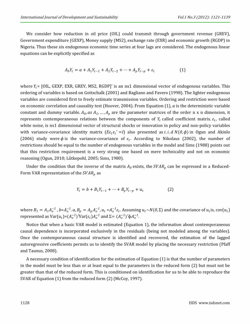
We consider how reduction in oil price (OIL) could transmit through government revenue (GREV),

Government expenditure (GEXP), Money supply (MS2), exchange rate (EXR) and economic growth (RGDP) in

Nigeria. Thus these six endogenous economic time series at four lags are considered. The endogenous linear

equations can be explicitly specified as

𝐴0𝑌𝑡 = 𝑎 + 𝐴1𝑌𝑡−1 + 𝐴2𝑌𝑡−2 + ⋯ + 𝐴𝑝𝑌𝑡−𝑝 + 𝜀𝑡 (1)

where 𝑌𝑡= [OIL, GEXP, EXR, GREV, MS2, RGDP]’ is an nx1 dimensional vector of endogenous variables. This

ordering of variables is based on Gottschalk (2001) and Bagliano and Favero (1998). The lighter endogenous

variables are considered first to freely estimate transmission variables. Ordering and restriction were based

on economic correlation and causality test (Hoover, 2004). From Equation (1), 𝑎 is the deterministic variable

constant and dummy variable. 𝐴0, 𝑎𝑠 𝐴1, … , 𝐴𝑝 are the parameter matrices of the order n x n dimension, it

represents contemporaneous relations between the components of 𝑌𝑡 called coefficient matrix. 𝜀𝑡 , called

white noise, is nx1 dimensional vector of structural shocks or innovation in policy and non-policy variables

with variance-covariance identity matrix (E𝜀𝑡𝜀𝑡 ʹ =I) also presented as 𝑖. 𝑖. 𝑑 𝑁(0,ɸ) in Ogun and Akinlo

(2006) study were ɸ is the variance-covariance of 𝜀𝑡 . According to Nikolaus (2002), the number of

restrictions should be equal to the number of endogenous variables in the model and Sims (1988) points out

that this restriction requirement is a very strong one based on mere technicality and not on economic

reasoning (Ogun, 2010; Lǘtkepohl, 2005; Sims, 1980).

Under the condition that the inverse of the matrix 𝐴0 exists, the 𝑆𝑉𝐴𝑅𝑝 can be expressed in a Reduced-

Form VAR representation of the 𝑆𝑉𝐴𝑅𝑝 as

𝑌𝑡 = 𝑏 + 𝐵1𝑌𝑡−1 + ⋯ + 𝐵𝑝𝑌𝑡−𝑝 + 𝑢𝑡 (2)

where 𝐵1 = 𝐴1𝐴𝑜−1 , b=𝐴𝑜

−1. 𝑎, 𝐵𝑝 = 𝐴𝑝𝐴𝑜−1, 𝑢𝑡 =𝐴𝑜

−1𝜀𝑡 . Assuming 𝑢𝑡~𝑁(0, Σ) and the covariance of 𝑢𝑡 is, cov(𝑢𝑡)

represented as Var(𝑢𝑡)=(𝐴𝑜−1)′Var(𝜀𝑡)𝐴𝑜

−1 and Σ= (𝐴𝑜−1)′ɸ𝐴𝑜

−1.

Notice that when a basic VAR model is estimated (Equation 1), the information about contemporaneous

causal dependence is incorporated exclusively in the residuals (being not modeled among the variables).

Once the contemporaneous causal structure is identified and recovered, the estimation of the lagged

autoregressive coefficients permits us to identify the SVAR model by placing the necessary restriction (Pfaff

and Taunus, 2008).

A necessary condition of identification for the estimation of Equation (1) is that the number of parameters

in the model must be less than or at least equal to the parameters in the reduced form (2) but must not be

greater than that of the reduced form. This is conditioned on identification for us to be able to reproduce the

SVAR of Equation (1) from the reduced form (2) (McCoy, 1997).



For the fact that the equations may not follow a unique form, imposition of restrictions is necessary.

Notice that there are more unobserved parameters in Equation (1) whose number amounts to n2(p + 1), than

parameters that can be estimated from Equation (2), which are n2p in the parameters of the Reduced-Form.

So we impose at least n (n − 1)/2 restrictions on the system, were n is the number of variables (Alessio, 2011

and Ogun, 2010).

More explicitly, from our Equation 1, 𝑌𝑡 is nx1 dimensional vector, the SVAR (1) has n, (p+1)n2 and

n(n+1)/2 parameters in the deterministic term a, the coefficient matrix, (𝐴0, 𝐴1 ………, 𝐴𝑝) and the

covariance matrix ɸ respectively. In sum our SVAR (Equation 1) is [n + (p+1)n2+ n(n+1)/2].

For the reduced-form VAR of (2), there are n, n2p and n(n+1)/2 parameters in the deterministic term,

coefficient matrix 𝐵𝑖 and cov(𝑢𝑡) represented as Σ= (𝐴𝑜−1)ʹɸ𝐴𝑜

−1matrix that is symmetric and positive

definite. In sum, (2) is n+n2p+n(n+1)/2.

Comparing SVARp with that of the reduced form VAR thus;

[n +(p+1)n2+n(n+1)/2] – [n+n2p+n(n+1)/2] =n2

It is worth noting that the main difference between the SVAR and the reduced form model above is in the

coefficient matrix. Since the SVAR (1) is greater than (2) reduced form model, there is the problem of

identification. That is, Equation (1) is under-identified, implying that the reduced form model (2) maybe

compatible with different structural equations. This necessitates the call for the imposition of the difference

(n2) restrictions (Sims, 1980). Hence, the identification of the SVARp requires minimum restriction of the

covariance matrix (ɸ) to n(n-1)/2 or on the matrix A0 zero restrictions on (Pfaff and Taunus, 2008; Hoover,

2004).

Assuming normality of the unobservable structural shocks, the residuals may then be mapped into

structural shocks. Normalising the variance to one and imposing orthogonality across the structural shocks,

i.e. ɸ = 1n, then Σ= 𝐴𝑜−1 𝐴𝑜

−1 ʹ (Nikolaus, 2011). The inverse of Aocould be ∆, and Σ= ∆∆ʹ (Ogun and Akinlo,

2006).

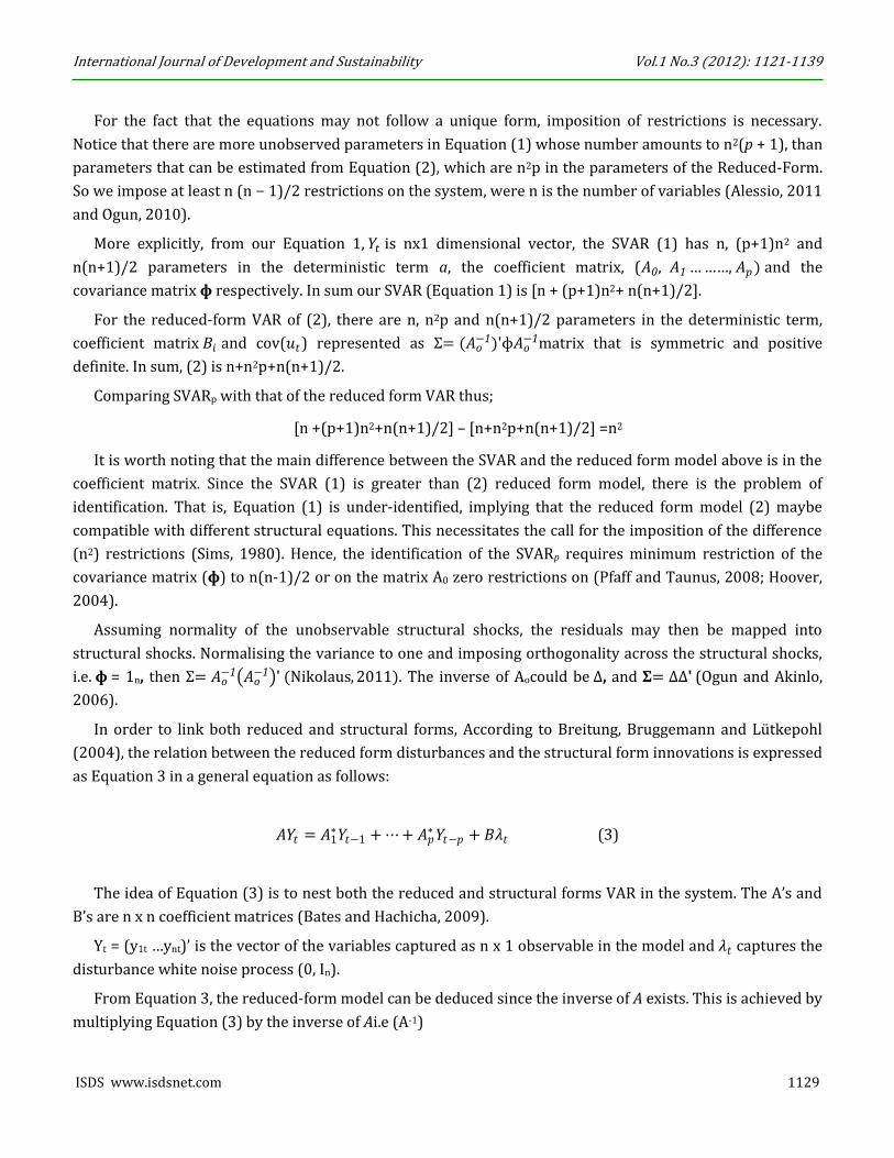
In order to link both reduced and structural forms, According to Breitung, Bruggemann and Lütkepohl

(2004), the relation between the reduced form disturbances and the structural form innovations is expressed

as Equation 3 in a general equation as follows:

𝐴𝑌𝑡 = 𝐴1∗𝑌𝑡−1 + ⋯ + 𝐴𝑝

∗𝑌𝑡−𝑝 + 𝐵𝜆𝑡 (3)

The idea of Equation (3) is to nest both the reduced and structural forms VAR in the system. The A’s and

B’s are n x n coefficient matrices (Bates and Hachicha, 2009).

Yt = (y1t …ynt)’ is the vector of the variables captured as n x 1 observable in the model and 𝜆𝑡 captures the

disturbance white noise process (0, In).

From Equation 3, the reduced-form model can be deduced since the inverse of A exists. This is achieved by

multiplying Equation (3) by the inverse of Ai.e (A-1)



𝑌𝑡 = 𝑧0 + 𝑧1𝑌𝑡−1 + ⋯ + 𝑧𝑝𝑌𝑡−𝑝 + 𝑣𝑡 (4)

𝑧𝑖=A-1𝐴𝑖∗ (𝑖 = 0, 1 …𝑝) and 𝑣𝑡 = 𝐵𝜆𝑡A-1

The relationship between the reduced-form VAR residual (𝑣𝑡) and the SVAR residual (𝐵𝜆𝑡) is called the

AB-model and presented below.

𝑣𝑡 =A-1B𝜆𝑡 or can be alternatively written as A𝑣𝑡=𝐵𝜆𝑡 . The variance-covariance matrix also called the

maximum likelihood estimator of the reduced form model can now be expressed as Σ= 𝐴𝑜−1BB′ 𝐴𝑜

−1 ʹor 𝐵𝐵′

given that 𝐴 = 𝐴0 and that 𝐴𝑜−1 𝐴𝑜

−1 ʹ = 1 (Pfaff and Taunus, 2008).

From the above, the identification problem is solved by imposing restrictions on the A and B matrices

assumed to be nonsingular. When B = In, we have A model as the required restrictions can now be imposed

on the contemporaneous residual of matrix A in the AB-model in the Jmulti software.

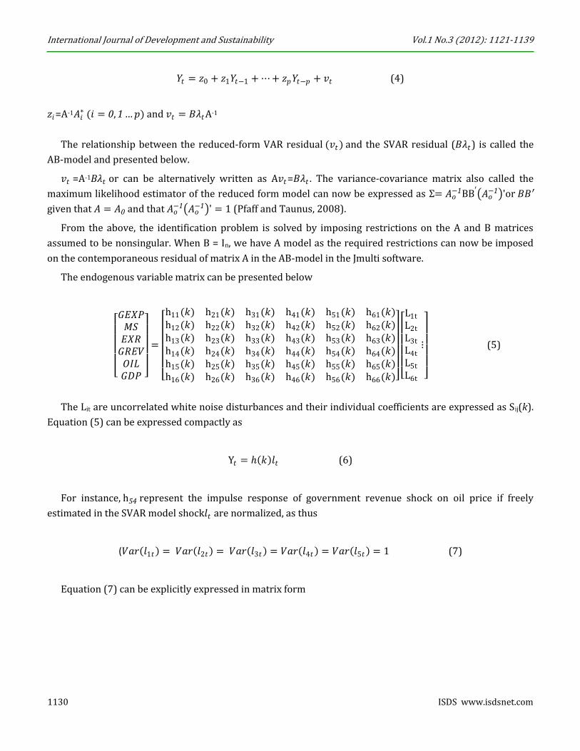
The endogenous variable matrix can be presented below

𝐺𝐸𝑋𝑃𝑀𝑆𝐸𝑋𝑅𝐺𝑅𝐸𝑉𝑂𝐼𝐿𝐺𝐷𝑃

=

h11(𝑘) h21(𝑘) h31(𝑘) h41(𝑘) h51(𝑘) h61(𝑘)h12(𝑘) h22(𝑘) h32(𝑘) h42(𝑘) h52(𝑘) h62(𝑘)h13(𝑘) h23(𝑘) h33(𝑘) h43(𝑘) h53(𝑘) h63(𝑘)h14(𝑘) h24(𝑘) h34(𝑘) h44(𝑘) h54(𝑘) h64(𝑘)h15(𝑘) h25(𝑘) h35(𝑘) h45(𝑘) h55(𝑘) h65(𝑘)h16(𝑘) h26(𝑘) h36(𝑘) h46(𝑘) h56(𝑘) h66(𝑘)

L1t

L2t

L3t

L4t

L5t

L6t

⋮

(5)

The Lit are uncorrelated white noise disturbances and their individual coefficients are expressed as Sij(k).

Equation (5) can be expressed compactly as

Y𝑡 = ℎ 𝑘 𝑙𝑡 (6)

For instance, h54 represent the impulse response of government revenue shock on oil price if freely

estimated in the SVAR model shock𝑙𝑡 are normalized, as thus

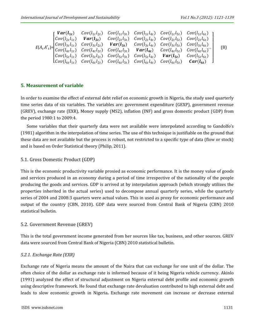
(𝑉𝑎𝑟 𝑙1𝑡 = 𝑉𝑎𝑟 𝑙2𝑡 = 𝑉𝑎𝑟 𝑙3𝑡 = 𝑉𝑎𝑟 𝑙4𝑡 = 𝑉𝑎𝑟 𝑙5𝑡 = 1 (7)

Equation (7) can be explicitly expressed in matrix form



E(𝐴𝑡𝐴′𝑡 )=

𝑽𝒂𝒓(𝒍𝟏𝒕) 𝐶𝑜𝑣(𝑙1𝑡𝑙2𝑡) 𝐶𝑜𝑣(𝑙1𝑡 𝑙3𝑡) 𝐶𝑜𝑣(𝑙1𝑡 𝑙4𝑡) 𝐶𝑜𝑣(𝑙1𝑡𝑙5𝑡) 𝐶𝑜𝑣(𝑙1𝑡𝑙6𝑡)

𝐶𝑜𝑣(𝑙2𝑡𝑙1𝑡) 𝑽𝒂𝒓(𝒍𝟐𝒕) 𝐶𝑜𝑣(𝑙2𝑡 𝑙3𝑡) 𝐶𝑜𝑣(𝑙2𝑡 𝑙4𝑡) 𝐶𝑜𝑣(𝑙2𝑡 𝑙5𝑡) 𝐶𝑜𝑣(𝑙2𝑡𝑙6𝑡)𝐶𝑜𝑣(𝑙3𝑡𝑙1𝑡) 𝐶𝑜𝑣(𝑙3𝑡𝑙2𝑡) 𝑽𝒂𝒓(𝒍𝟑𝒕) 𝐶𝑜𝑣(𝑙3𝑡 𝑙4𝑡) 𝐶𝑜𝑣(𝑙3𝑡 𝑙5𝑡) 𝐶𝑜𝑣(𝑙3𝑡𝑙6𝑡)𝐶𝑜𝑣(𝑙4𝑡𝑙1𝑡) 𝐶𝑜𝑣(𝑙4𝑡𝑙2𝑡) 𝐶𝑜𝑣(𝑙4𝑡 𝑙3𝑡) 𝑽𝒂𝒓(𝒍𝟒𝒕) 𝐶𝑜𝑣(𝑙4𝑡 𝑙5𝑡) 𝐶𝑜𝑣(𝑙4𝑡𝑙6𝑡)𝐶𝑜𝑣(𝑙5𝑡𝑙1𝑡) 𝐶𝑜𝑣(𝑙5𝑡𝑙2𝑡) 𝐶𝑜𝑣(𝑙5𝑡 𝑙3𝑡) 𝐶𝑜𝑣(𝑙5𝑡 𝑙4𝑡) 𝑽𝒂𝒓(𝒍𝟓𝒕) 𝐶𝑜𝑣(𝑙5𝑡𝑙6𝑡)𝐶𝑜𝑣(𝑙6𝑡𝑙1𝑡) 𝐶𝑜𝑣(𝑙6𝑡𝑙2𝑡) 𝐶𝑜𝑣(𝑙6𝑡 𝑙3𝑡) 𝐶𝑜𝑣(𝑙6𝑡 𝑙4𝑡) 𝐶𝑜𝑣(𝑙6𝑡 𝑙5𝑡) 𝑪𝒂𝒓(𝒍𝟔𝒕)

. .

(8)

5. Measurement of variable

In order to examine the effect of external debt relief on economic growth in Nigeria, the study used quarterly

time series data of six variables. The variables are: government expenditure (GEXP), government revenue

(GREV), exchange rate (EXR), Money supply (MS2), inflation (INF) and gross domestic product (GDP) from

the period 1980:1 to 2009:4.

Some variables that their quarterly data were not available were interpolated according to Gandolfo’s

(1981) algorithm in the interpolation of time series. The use of this technique is justifiable on the ground that

these data are not available but the process is robust, not restricted to a specific type of data (flow or stock)

and is based on Order Statistical theory (Philip, 2011).

5.1. Gross Domestic Product (GDP)

This is the economic productivity variable proxied as economic performance. It is the money value of goods

and services produced in an economy during a period of time irrespective of the nationality of the people

producing the goods and services. GDP is arrived at by interpolation approach (which strongly utilizes the

properties inherited in the actual series) used to decompose annual quarterly series, while the quarterly

series of 2004 and 2008:3 quarters were actual values. This in used as proxy for economic performance and

output of the country (CBN, 2010). GDP data were sourced from Central Bank of Nigeria (CBN) 2010

statistical bulletin.

5.2. Government Revenue (GREV)

This is the total government income generated from her sources like tax, business, and other sources. GREV

data were sourced from Central Bank of Nigeria (CBN) 2010 statistical bulletin.

5.2.1. Exchange Rate (EXR)

Exchange rate of Nigeria means the amount of the Naira that can exchange for one unit of the dollar. The

often choice of the dollar as exchange rate is informed because of it being Nigeria vehicle currency. Akinlo

(1991) analyzed the effect of structural adjustment on Nigeria external debt profile and economic growth

using descriptive framework. He found that exchange rate devaluation contributed to high external debt and

leads to slow economic growth in Nigeria. Exchange rate movement can increase or decrease external



obligations of a debtor country especially when the debt is serviced in foreign currency. Here the official

exchange rate of the Naira is used as the exchange rate as government transactions are based on it. EXR data

were sourced from Central Bank of Nigeria (CBN) 2010 statistical bulletin.

In general, the main sources of data for the study include Central Bank of Nigeria-Statistical Bulletin

(various issues) and Annual Report and Statement of Accounts (various issues). To appraise the transmission

mechanism between external debt relief and economic growth in Nigeria was achieved through SVAR

method.

In the estimation procedure as highlighted by Alessio (2011), the VAR model is first estimated after the

usual specification; Lags and unit root tests. If the non-stationarity hypothesis is rejected, we estimate the

VAR by OLS. The Vector Error Correction Method (VECM) is to be used if there is unit root in the time series

and the test for cointegration relationships exist. But if they do not cointegrate, we estimate the VAR by

taking first difference.

Following Benkwitz et al. (2001), some small sample properties of bootstrap confidence intervals are

better in comparison to other asymptotic methodologies. Bootstrap percentile 95% confidence intervals are

computed to illustrate parameter uncertainty. The percentile method proposed in Hall (1992) is used with

1000 replications.

This would lead to the estimation of the SVAR, were we apply our restrictions to show transmissions of

shock through Impulse Response Functions (IRFs) and Forecast Error Variance Decomposition (FEVD). The

IRF trace out the response of current and future values of each of the variables to a unit innovation/shock in

the current value of the VAR disturbances. For example, h45 in Equation 5 captures the impulse response of

RGDP shock on oil price (Pfaff and Taunus, 2008).

VAR model can be applied in levels or in first differencing according to Pesaran and Pesaran (1997). This

study adopts the SVAR in estimating the transmission of oil price on fiscal variables.

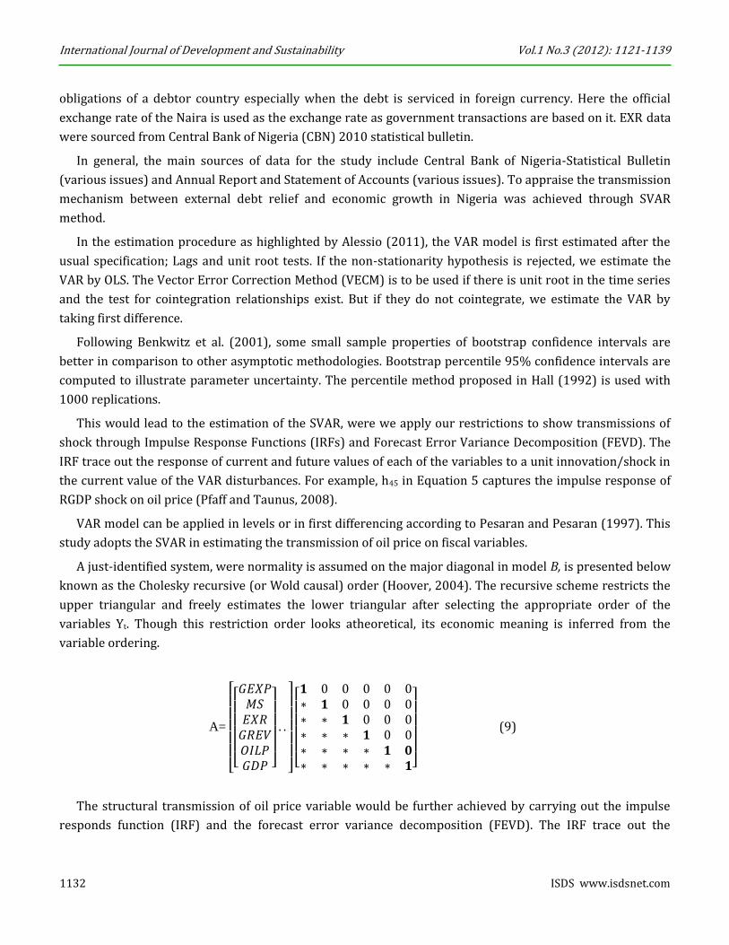
A just-identified system, were normality is assumed on the major diagonal in model B, is presented below

known as the Cholesky recursive (or Wold causal) order (Hoover, 2004). The recursive scheme restricts the

upper triangular and freely estimates the lower triangular after selecting the appropriate order of the

variables Yt. Though this restriction order looks atheoretical, its economic meaning is inferred from the

variable ordering.

A=

𝐺𝐸𝑋𝑃𝑀𝑆𝐸𝑋𝑅𝐺𝑅𝐸𝑉𝑂𝐼𝐿𝑃𝐺𝐷𝑃

. .

𝟏 0 0 0 0 0∗ 𝟏 0 0 0 0∗ ∗ 𝟏 0 0 0∗ ∗ ∗ 𝟏 0 0∗ ∗ ∗ ∗ 𝟏 𝟎∗ ∗ ∗ ∗ ∗ 𝟏

(9)

The structural transmission of oil price variable would be further achieved by carrying out the impulse

responds function (IRF) and the forecast error variance decomposition (FEVD). The IRF trace out the



response of current and future values of the variable freely estimated to a one-standard error shock in the

current value of one of the VAR errors. On the other hand, the FEVD indicates the percentage of the variance

of the error made in forecasting a variable due to a specific shock at a given horizon.

6. Data analysis and discussion of result

6.1. Unit root test

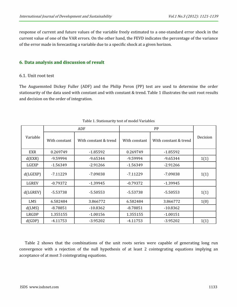
The Auguemnted Dickey Fuller (ADF) and the Philip Peron (PP) test are used to determine the order

stationarity of the data used with constant and with constant & trend. Table 1 illustrates the unit root results

and decision on the order of integration.

Table 1. Stationarity test of model Variables

Variable

ADF PP

Decision With constant With constant & trend With constant With constant & trend

EXR 0.269749 -1.85592 0.269749 -1.85592

d(EXR) -9.59994 -9.65344 -9.59994 -9.65344 1(1)

LGEXP -1.56349 -2.91266 -1.56349 -2.91266

d(LGEXP) -7.11229 -7.09038 -7.11229 -7.09038 1(1)

LGREV -0.79372 -1.39945 -0.79372 -1.39945

d(LGREV) -5.53738 -5.50553 -5.53738 -5.50553 1(1)

LMS 6.582484 3.866772 6.582484 3.866772 1(0)

d(LMS) -8.78851 -10.8362 -8.78851 -10.8362

LRGDP 1.355155 -1.00156 1.355155 -1.00151

d(GDP) -4.11753 -3.95202 -4.11753 -3.95202 1(1)

Table 2 shows that the combinations of the unit roots series were capable of generating long run

convergence with a rejection of the null hypothesis of at least 2 cointegrating equations implying an

acceptance of at most 3 cointegrating equations.



Table 2. Johansen Cointegration Test

Model 1: Series: EXR GEXP INFLRT LRGDP LRPCEC

Hypothesised Eigenvalue Trace 0.05 Critical Prob**

No of Ces

Statistic Value

None * 0.447 166.663 95.754 0.000

At most 1 * 0.329 97.426 69.819 0.000

At most 2 * 0.182 50.840 47.856 0.026

At most 3 0.141 27.369 29.797 0.093

At most 4 0.070 9.648 15.495 0.309

At most 5 0.010 1.118 3.842 0.290

Trace test indicates 3 cointegratingeqn(s) at the 0.05 level

* denotes rejection of the hypothesis at the 0.05 level

**MacKinnon-Haug-Michelis (1999) p-values

6.2. SVAR impulse response results

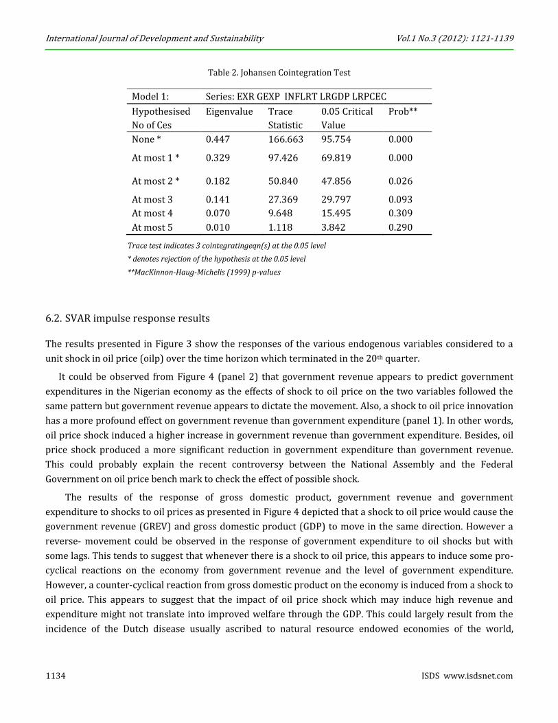
The results presented in Figure 3 show the responses of the various endogenous variables considered to a

unit shock in oil price (oilp) over the time horizon which terminated in the 20th quarter.

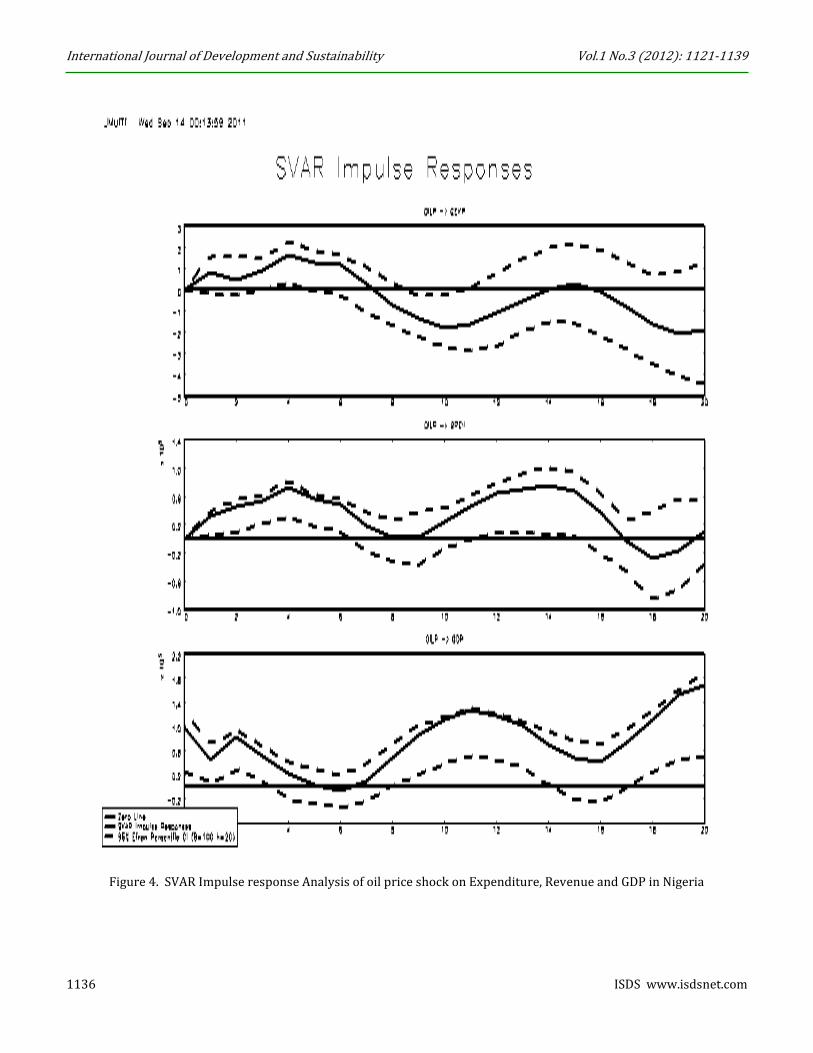
It could be observed from Figure 4 (panel 2) that government revenue appears to predict government

expenditures in the Nigerian economy as the effects of shock to oil price on the two variables followed the

same pattern but government revenue appears to dictate the movement. Also, a shock to oil price innovation

has a more profound effect on government revenue than government expenditure (panel 1). In other words,

oil price shock induced a higher increase in government revenue than government expenditure. Besides, oil

price shock produced a more significant reduction in government expenditure than government revenue.

This could probably explain the recent controversy between the National Assembly and the Federal

Government on oil price bench mark to check the effect of possible shock.

The results of the response of gross domestic product, government revenue and government

expenditure to shocks to oil prices as presented in Figure 4 depicted that a shock to oil price would cause the

government revenue (GREV) and gross domestic product (GDP) to move in the same direction. However a

reverse- movement could be observed in the response of government expenditure to oil shocks but with

some lags. This tends to suggest that whenever there is a shock to oil price, this appears to induce some pro-

cyclical reactions on the economy from government revenue and the level of government expenditure.

However, a counter-cyclical reaction from gross domestic product on the economy is induced from a shock to

oil price. This appears to suggest that the impact of oil price shock which may induce high revenue and

expenditure might not translate into improved welfare through the GDP. This could largely result from the

incidence of the Dutch disease usually ascribed to natural resource endowed economies of the world,



particularly the less developed countries, which has been widely established in the literature (see Olomola

and Adejumo, 2006 and Anty, 2001).

Figure 3. SVAR Impulse response Analysis of oil price shock in Nigeria

The above observations to a considerable extent suggest that the behavior of fiscal variables of

government expenditure and government revenue is greatly conditioned by oil price shocks. This finding is

in line with the previous study of Davis (1987) who argued that oil price shocks explain much of the time

series variations of fiscal variables.

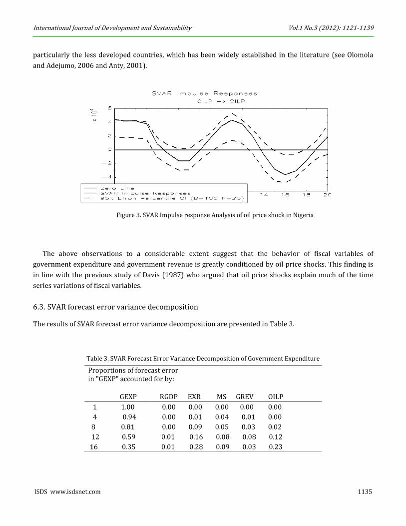
6.3. SVAR forecast error variance decomposition

The results of SVAR forecast error variance decomposition are presented in Table 3.

Table 3. SVAR Forecast Error Variance Decomposition of Government Expenditure

Proportions of forecast error in "GEXP" accounted for by:

GEXP RGDP EXR MS GREV OILP

1 1.00 0.00 0.00 0.00 0.00 0.00

4 0.94 0.00 0.01 0.04 0.01 0.00

8 0.81 0.00 0.09 0.05 0.03 0.02

12 0.59 0.01 0.16 0.08 0.08 0.12

16 0.35 0.01 0.28 0.09 0.03 0.23



Figure 4. SVAR Impulse response Analysis of oil price shock on Expenditure, Revenue and GDP in Nigeria



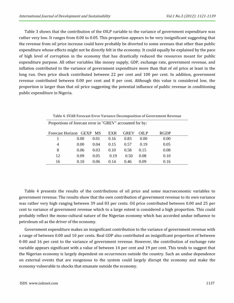
Table 3 shows that the contribution of the OILP variable to the variance of government expenditure was

rather very low. It ranges from 0.00 to 0.05. This proportion appears to be very insignificant suggesting that

the revenue from oil price increase could have probably be diverted to some avenues that other than public

expenditure whose effects might not be directly felt in the economy. It could equally be explained by the pace

of high level of corruption in the economy that has drastically reduced the resources meant for public

expenditure purpose. All other variables like money supply, GDP, exchange rate, government revenue, and

inflation contributed to the variance of government expenditure more than that of oil price at least in the

long run. Own price shock contributed between 22 per cent and 100 per cent. In addition, government

revenue contributed between 0.00 per cent and 8 per cent. Although this value is considered low, the

proportion is larger than that oil price suggesting the potential influence of public revenue in conditioning

public expenditure in Nigeria.

Table 4. SVAR Forecast Error Variance Decomposition of Government Revenue

Proportions of forecast error in "GREV" accounted for by:

Forecast Horizon GEXP MS EXR GREV OILP RGDP

1 0.00 0.01 0.16 0.83 0.00 0.00

4 0.00 0.04 0.15 0.57 0.19 0.05

8 0.06 0.03 0.10 0.58 0.15 0.08

12 0.09 0.05 0.19 0.50 0.08 0.10

16 0.10 0.06 0.14 0.46 0.09 0.16

Table 4 presents the results of the contributions of oil price and some macroeconomic variables to

government revenue. The results show that the own contribution of government revenue to its own variance

was rather very high ranging between 39 and 83 per cents. Oil price contributed between 0.00 and 25 per

cent to variance of government revenue which to a large extent is considered a high proportion. This could

probably reflect the mono-cultural nature of the Nigerian economy which has accorded undue influence to

petroleum oil as the driver of the economy.

Government expenditure makes an insignificant contribution to the variance of government revenue with

a range of between 0.00 and 10 per cents. Real GDP also contributed an insignificant proportion of between

0-00 and 16 per cent to the variance of government revenue. However, the contribution of exchange rate

variable appears significant with a value of between 14 per cent and 19 per cent. This tends to suggest that

the Nigerian economy is largely dependent on occurrences outside the country. Such an undue dependence

on external events that are exogenous to the system could largely disrupt the economy and make the

economy vulnerable to shocks that emanate outside the economy.



7. Conclusion and policy implication

The facts that emerged from the above analysis suggest that oil price shocks have a lot of influence on the

management of the Nigerian economy. The shocks to oil price to a large extent have great influence on the

level of government revenue which ultimately influenced the level of government expenditure in the

Nigerian economy. A shocking revelation from the analysis shows that despite the fact that oil price

contributed to government revenue, such an increase did not proportionally translate to increase in

government expenditure. It could therefore be inferred from this that there some resources are probably

being misappropriated instead of being engaged in productive fiscal activities for economic growth.

On the basis of the above analysis, it is suggested that the government should be sensitive to the fact that

oil price shock could have great influence on the Nigerian economy. The government should therefore take

steps to ensure that any unforeseen influences resulting from the vagaries from oil price shocks are guarded

against. Besides, the government should not totally rely on the windfalls from oil price shocks in making

economic forecast as this could be dangerous to the economy, rather other sources of revenues should be

explored to complement the revenues from oil price shocks. In addition, government should initiate

appropriate measures to ensure that additional revenues realized from the oil price shocks are properly

utilized to pursue developmental objectives.

References

Manzano .O and Rigobon R. (2001), “Resource Curse or Debt Overhang?”, NBER Working Paper No. w8390,

July.

Mehrara M. and Oskoui K.N. (2007), “The Sources of Macroeconomic Fluctuations in Oil Exporting Countries:

A comparative study”, Economic Modelling, Vol. 24 No. 3, pp. 365-379.

Merlevede B., Schoors, K. J. L. and Van Aarle B. (2009), “Russia from Bust to Boom and Back: Oil Price, Dutch

Disease and Stabilization Fund”, Comparative Economic Studies, Vol. 51, No. 2, pp. 213-241,

Montenegro, S. (1994), "Macroeconomic Risk Management in Nigeria: Dealing with External Shocks",

available at: http://siteresources.worldbank.org/INTFINDINGS/685507-1161268713892/21098561/find30.

htm.

Ogun, T.P. and Akinlo, A.E. (2006), “The Effectiveness of Bank Credit Channel of Monetary Policy

Transmission: the Nigerian Experience”, African Economic and Business Review, Vol. 8 No. 2.

Olomola P.A. (2006), “Oil price shock and Macroeconomic Activities in Nigeria”, International Research

Journal of Finance and Economics, No. 3.

Olusegun, O.A., (2008), “Oil price shocks and the Nigerian economy: A forecast error variance decomposition

Analysis”, J. Economic Theory, Vol. 2, pp. 124-130.

http://papers.ssrn.com/sol3/cf_dev/AbsByAuth.cfm?per_id=141109




http://siteresources.worldbank.org/INTFINDINGS/685507-1161268713892/21098561/find30.htm

http://siteresources.worldbank.org/INTFINDINGS/685507-1161268713892/21098561/find30.htm



Omisakin, O., Adeniyi, O. and Omojolaibi, A. (2009), “A vector Error Correction Modeling of Energy Price

Volatilty of a Dependent Economy: The case of Nigeria”, Parkistan Journal of Social Sciences, Vol. 6 No. 4, pp.

207-213.

Pieschacon A. (2009), “Oil Booms and their Impacts through Fiscal Policy”, available at: http://scid-

new.stanford.edu/system/files/shared/Pieschacon_5-01-09.pdf, accessed 10 February 2013.

Ross, Michael L. (2001a), “Does Oil Hinder Democracy?” World Politics, Vol. 53 (3, April), pp. 325-361.

Sachs, J.D. and Andrew M.W. (1997), “Natural Resource Abundance and Economic Growth”, Harvard Institute

for International Development, Cambridge, Development Discussion Paper No. 517a.

Sachs, J.D. & Warner, A. M. (2001), “The curse of natural resources”, European Economic Review, Vol. 45, No.

4-6, pp. 827-838.

Sachs, Jeffrey D. & Warner, Andrew M. (1999), “The big push, natural resource booms and growth”, Journal of

Development Economics, Elsevier, Vol. 59 No. 1, pp. 43-76.

Schubert, S.F. (2009), “Dynamic Effects of Oil Price Shocks and their Impact on the Current Account”, Free

University of Bozen-Bolzano, O Munich Personal RePEc Archive.

Sims, C. A. (1980), “Macroeconomics and Reality in Econometrica”, Econometrica is currently published by The

Econometric Society, Vol. 48 No. 1, pp. 1-48.

Sims, C. A. (1988), Identifying policy effect in R. C. Bryant, ed., Empirical Macroeconomics for Interdependent

Economies', Brookings Institution, Washington DC, pp. 305-321.

Sturm, M, Gurtner, F and J.G Alegre, (2009) ‘Fiscal policy challenges in oil-exporting countries a review of key

issues’. Occasional Paper Series, European Central Bank No 104 / June.

Umar G. and Abdulhakeem K. (2010), “Oil Price Shocks and the Nigeria Economy: A Variance Autoregressive

(VAR) Model”, International Journal of Business and Management Vol. 5, No. 8.

United Nations (2005), ‘The Exposure of African Governments to International oil Volatility and what to do

about it’. United Nations Conference on Trade and Development. Geneva. December

Wikipedia (2011), ‘Economy of Nigeria’ the free Encyclopedia. March.

World Bank (2001), ‘World Development Report 2000/2001: Attacking Poverty’, New York: World Bank and

Oxford University Press.

World Bank (2004), ‘The Effects of Oil Shocks on the Economy: A Review of the Empirical Evidence’. Report

for Congress, Congressional Research Service. The Library of Congress.

World Bank (2010), ‘Country Level Evaluation Nigeria’. Final Report, Volume II: Annexes.Evaluation carried

out on behalf of the European Commission.

Documents

Oil price shocks and fiscal policy management ... · Since 1970s there have been five main negative oil shocks. The first was from 1973 to 1974 whose fluctuation was as a result of