Embed Size (px)
Citation preview
8/8/2019 Oguntade Ayoade Range Estimation for Tactical Radio Waveforms Using Link Budget Analysis
http://slidepdf.com/reader/full/oguntade-ayoade-range-estimation-for-tactical-radio-waveforms-using-link-budget 1/100
A Thesis
Entitled
Range Estimation for Tactical Radio Waveforms using
Link Budget Analysis
by
Ayoade Oguntade
Submitted as partial fulfillment of the requirements for
the Master of Science in Electrical Engineering
___________________________________ Dr. Junghwan Kim, Committee Chair
___________________________________ Dr. Lawrence Miller, Committee Member
___________________________________
Dr. Ezzatollah Salari, Committee Member
___________________________________
Dr. Patricia R. Komuniecki, Dean
College of Graduate Studies
The University of Toledo
May 2010

8/8/2019 Oguntade Ayoade Range Estimation for Tactical Radio Waveforms Using Link Budget Analysis
http://slidepdf.com/reader/full/oguntade-ayoade-range-estimation-for-tactical-radio-waveforms-using-link-budget 2/100

8/8/2019 Oguntade Ayoade Range Estimation for Tactical Radio Waveforms Using Link Budget Analysis
http://slidepdf.com/reader/full/oguntade-ayoade-range-estimation-for-tactical-radio-waveforms-using-link-budget 3/100
iii
An Abstract of
Range Estimation for Tactical Radio Waveforms using Link Budget Analysis
by
Ayoade Oguntade
Submitted as partial fulfillment of the requirements for
the Master of Science in Electrical Engineering
The University of Toledo
May 2010
The increasing need to design multiband tactical radio communication modems
that will incorporate several waveforms has made the investigation of the performance of
different tactical waveforms absolutely necessary. These different waveforms must also
meet various demands in quality and nature of data. Range maximization, high data
throughput, and power conservation requirements are usually not fulfilled by a single
waveform. To effectively deliver tactical multimedia data including coded audio, text,
video, map, and navigation information using radio, multiple choice of frequency bands
exist. These include: HF, VHF and UHF. However, along with the effective delivery of
quality data, the maximization of transmission range under hostile propagation
environments – especially under terrain blockage in ground-to-ground (GTG)

8/8/2019 Oguntade Ayoade Range Estimation for Tactical Radio Waveforms Using Link Budget Analysis
http://slidepdf.com/reader/full/oguntade-ayoade-range-estimation-for-tactical-radio-waveforms-using-link-budget 4/100
iv
communication scenario - is of utmost importance. This thesis discusses the results of
Link Budget Analysis (LBA) performed for the estimation of maximum delivery range of
tactical radio waveforms using variety of data rates for three typically different
waveforms – High Frequency Waveform (HFW), Very High Frequency Waveform
(VHFW) and OFDM based Wideband Network Waveform (WNW). Center frequencies
of 27 MHz, 60 MHz, and 500 MHz respectively were used for the simulations.
Results show that HFW produces the longest range, followed by VHFW and the
WNW – which delivered the highest data rate. Also, the amount of variation in
propagation range that was noticed while parameters like center frequency, antenna
height, antenna gain, transmitter power were varied were also computed.

8/8/2019 Oguntade Ayoade Range Estimation for Tactical Radio Waveforms Using Link Budget Analysis
http://slidepdf.com/reader/full/oguntade-ayoade-range-estimation-for-tactical-radio-waveforms-using-link-budget 5/100
v
To my Parents: Emmanuel and Rachel

8/8/2019 Oguntade Ayoade Range Estimation for Tactical Radio Waveforms Using Link Budget Analysis
http://slidepdf.com/reader/full/oguntade-ayoade-range-estimation-for-tactical-radio-waveforms-using-link-budget 6/100
vi
Acknowledgements
I would like to express profound gratitude to my advisor, Dr. Junghwan Kim, for
his unstinting support, encouragement, supervision and valuable suggestions throughout
this research work. I would also like to thank the entire members of the Communications
Lab for their advice.
Special thanks also go to the local chapter of the National Society of Black
Engineers (NSBE UT) for their support and friendship throughout my stay at UT. I am
also grateful for the opportunity to serve as an executive of this academically-enriching
organization.
I sincerely appreciate Professor Salari and Professor Miller for serving as
members of my thesis defense committee.
Finally, I would also like to deeply appreciate Professor Samuel Kassegne of San
Diego State University (SDSU) for his advice and Mentorship. I also appreciate Damilola
Olushola and Damilola Adewoye of the University of Cincinnati for their support in the
course of my program.

8/8/2019 Oguntade Ayoade Range Estimation for Tactical Radio Waveforms Using Link Budget Analysis
http://slidepdf.com/reader/full/oguntade-ayoade-range-estimation-for-tactical-radio-waveforms-using-link-budget 7/100
vii
Contents
Abstract......................................................................................................................................... iii
Acknowledgements ...................................................................................................................... vi
Table of Contents ......................................................................................................................... vi
List of Figures............................................................................................................................. viii
List of Tables................................................................................................................................. ix
1 Background - Wireless Radio .................................................................................................. 1
1.1 Motivation ............................................................................................................................. 31.2 Radio Channel ....................................................................................................................... 3
1.3 Thesis Contribution ............................................................................................................... 4
1.4 Thesis Outline ....................................................................................................................... 5
2 Waveform Design ....................................................................................................................... 6
2.1 High FrequencyWaveform .................................................................................................... 6
2.1.1 HFW Waveform Parameters .......................................................................................... 7
2.1.2 HFW FEC Coding .......................................................................................................... 8
2.2 Very High FrequencyWaveform .......................................................................................... 112.2.1 VHFW Waveform Parameters ..................................................................................... 12
2.2.2 VHFW FEC Coding ..................................................................................................... 15
2.3 Introduction to Windband Network Waveform (WNW) .................................................... 15
3 OFDM Basics and WNW ........................................................................................................ 16
3.1 Analogy of OFDM in real life ............................................................................................. 16
3.1.1 OFDM Principle ........................................................................................................... 17
3.2 Orthogonality of Subcarriers .............................................................................................. 173.2.1 Time Domain Explaination .......................................................................................... 18
3.2.2 Frequency Domain Expalination ................................................................................. 19
3.3 Generation of OFDM Subcarriers using IFFT .................................................................... 20
3.3.1 IFFT vs IDFT – Time Complexity ............................................................................... 213.4 ICI and ISI .......................................................................................................................... 21
3.5 Guard Time and Cyclic Prefix ............................................................................................ 223.6 Windowing .......................................................................................................................... 23
3.7 Wideband Network Waveform Parameters ......................................................................... 24
3.7.1 Forward Error Correction............................................................................................. 25
3.7.2 Interleaver .................................................................................................................... 263.7.3 Modulator ..................................................................................................................... 26

8/8/2019 Oguntade Ayoade Range Estimation for Tactical Radio Waveforms Using Link Budget Analysis
http://slidepdf.com/reader/full/oguntade-ayoade-range-estimation-for-tactical-radio-waveforms-using-link-budget 8/100
viii
3.7.4 Data Rate calculation ................................................................................................... 28
4 Channel Impairment Factors.................................................................................................. 30
4.1 Propagation Environment ................................................................................................... 30
4.1.1 Ground to Ground Open Terrain .................................................................................. 304.1.2 Ground to Ground Mountain Blockage ....................................................................... 31
4.1.3 Ground to Ground Urban Area .................................................................................... 324.1.4 Ship to Ground ............................................................................................................. 32
4.1.5 Ground to Ship ............................................................................................................. 334.1.6 Ship to Ship .................................................................................................................. 33
4.2 Path Loss Models ................................................................................................................ 34
4.2.1 Hata-Okomora Model .................................................................................................. 344.2.2 Egli Model ................................................................................................................... 36
4.2.3 GRWAVE Model .......................................................................................................... 37
4.2.4 Millington’s Model ...................................................................................................... 394.2.5 Lichun Model ............................................................................................................... 40
4.2.6 ITU-R Model ............................................................................................................... 42
4.2.7 Plane Earth Model ........................................................................................................ 444.3 Shadowing - Long Term Fading ......................................................................................... 454.4 Multipath – Short Term Fading ........................................................................................... 46
4.4.1 Rayleigh Fading Channel ............................................................................................. 46
4.4.2 Rician Fading Channel ................................................................................................. 474.4.3 Nakagami-m Channel .................................................................................................. 48
4.5 Other Fading Issues ............................................................................................................ 49
4.5.1 Frequency Flat and Frequency Selective Channels ..................................................... 494.5.2 Doppler Shift ................................................................................................................ 49
4.5.3 Coherence Time and Doppler Spread .......................................................................... 50
5 Link Budget Analysis ............................................................................................................... 51
5.1 Link Budget ........................................................................................................................ 51
5.2 Equipment Types ................................................................................................................ 515.2.1 Manpack Equipment .................................................................................................... 52
5.2.2 Vehicle Equipment ....................................................................................................... 52
5.3 Link Budget Parameters ...................................................................................................... 535.3.1 Transmitter Power ........................................................................................................ 53
5.3.2 Power Back off ............................................................................................................. 54
5.3.3 Center Frequency ......................................................................................................... 545.3.4 Antenna Height ............................................................................................................ 54
5.3.5 Antenna Gain ............................................................................................................... 555.3.6 Thermal Noise Power ................................................................................................... 55
5.3.7 Noise Figure ................................................................................................................. 555.3.8 Link Margin ................................................................................................................. 56
5.4 Sample Link Budget Analysis ............................................................................................. 57
5.4.1 Sample LBA calculation for GTG-O ........................................................................... 58

8/8/2019 Oguntade Ayoade Range Estimation for Tactical Radio Waveforms Using Link Budget Analysis
http://slidepdf.com/reader/full/oguntade-ayoade-range-estimation-for-tactical-radio-waveforms-using-link-budget 9/100
ix
6 Discussion of Results................................................................................................................ 61
6.1HFW Propagation Range ..................................................................................................... 62
6.1.1 HFW GTG-O ............................................................................................................... 62
6.1.2 HFW GTG-M ............................................................................................................... 636.1.3 HFW GTG-U ............................................................................................................... 64
6.1.4 HFW GTS/STG ............................................................................................................ 65
6.1.5 HFW STS ..................................................................................................................... 66
6.2 VHFW Propagation Range ................................................................................................ 676.2.1 VHFW GTG-O............................................................................................................. 67
6.2.2 VHFW GTG-M ............................................................................................................ 68
6.2.3 VHFW GTG-U............................................................................................................. 696.2.4 VHFW GTS/STG ......................................................................................................... 70
6.2.5 VHFW STS .................................................................................................................. 71
6.3WNW Propagation Range.................................................................................................... 72
6.3.1 WNW GTG-O .............................................................................................................. 736.3.2 WNW GTG-M ............................................................................................................. 74
6.3.3 WNW GTG-U .............................................................................................................. 75
6.3.4 WNW GTS/STG/STS .................................................................................................. 766.4 Propagation Range with design parameter variation .......................................................... 77
6.4.1 Range based on Environment and Data rate ................................................................ 77
6.4.2 Range based on Center Frequency ............................................................................... 796.4.3 Range based on Transmitter Power .............................................................................. 80
6.4.4 Range based on Antenna Height .................................................................................. 81
7 Conclusion and Future Work .................................................................................................. 83
7.1 Conclusion .......................................................................................................................... 847.2 Future Work ........................................................................................................................ 84
References .................................................................................................................................... 86

8/8/2019 Oguntade Ayoade Range Estimation for Tactical Radio Waveforms Using Link Budget Analysis
http://slidepdf.com/reader/full/oguntade-ayoade-range-estimation-for-tactical-radio-waveforms-using-link-budget 10/100
x
List of Figures
Figure 1.1 WNW in use in JTRS .................................................................................................... 2
Figure 2.1 BPSK Signal Constellation............................................................................................ 7
Figure 2.2 ½ Rate Convolution Encoder with memory order m = 2 for HFW ............................... 9
Figure 2.3 QPSK Signal Constellation ......................................................................................... 13
Figure 2.4 16-QAM Signal Constellation ..................................................................................... 14
Figure 2.5 32-QAM Signal Constellation ..................................................................................... 14
Figure 3.1 Parallel OFDM Subcarriers ......................................................................................... 17
Figure 3.2 Integer number of cycles over symbol peroid ............................................................. 18
Figure 3.3 Subcarriers in frequency domain ................................................................................. 19
Figure 3.4 Bandwidth savings by using overlapping orthogonal subcarriers ............................... 20
Figure 3.5 Time dispersion on OFDM system without Guard band. ............................................ 22
Figure 3.6 Time dispersion on OFDM system with Guard band and Cyclic Prefix ..................... 23
Figure 3.7 OFDM Symbol ............................................................................................................ 24
Figure 3.8 WNW Transmitter ....................................................................................................... 25
Figure 3.9 WNW Receiver ........................................................................................................... 25
Figure 3.10 BPSK Constellation ................................................................................................... 27
Figure 3.11 QPSK Constellation .................................................................................................. 27
Figure 3.12 16-QAM Constellation ............................................................................................. 28
Figure 4.1 Ground to Ground Open Terrain (GTG-O) ................................................................. 31
Figure 4.2 Ground to Ground Mountain Blockage (GTG-M) ...................................................... 32
Figure 4.3 Ground to Ground Urban Area (GTG-U) .................................................................... 32
Figure 4.4 WNW Ship to Ground (STG)/Ground to Ship (GTS) ................................................. 33
Figure 4.5 Screenshot of the GRWAVE model as used for HFW ................................................. 39
Figure 4.6 Eckersley and Millington’s Prediction methods .......................................................... 40

8/8/2019 Oguntade Ayoade Range Estimation for Tactical Radio Waveforms Using Link Budget Analysis
http://slidepdf.com/reader/full/oguntade-ayoade-range-estimation-for-tactical-radio-waveforms-using-link-budget 11/100
xi
Figure 4.7 Shadowing variation over different paths.................................................................... 45
Figure 5.1 Sample Link Budget Analysis ..................................................................................... 58
Figure 6.1 Range vs Data rate for HFW cases .............................................................................. 78
Figure 6.2 Range vs Data rate for VHFW Cases .......................................................................... 78
Figure 6.3 Range vs Data rate for WNW Cases ........................................................................... 79
Figure 6.4 Range vs Data rate for WNW GTG-U at different frequencies .................................. 80
Figure 6.5 Range vs Data rate for WNW GTG-U at different transmitter powers ....................... 81
Figure 6.6 Range vs Data rate for WNW GTG-U at different antenna heights ............................ 82

8/8/2019 Oguntade Ayoade Range Estimation for Tactical Radio Waveforms Using Link Budget Analysis
http://slidepdf.com/reader/full/oguntade-ayoade-range-estimation-for-tactical-radio-waveforms-using-link-budget 12/100
xii
List of Tables
Table 2.1 Mapping of Bits to BPSK Symbols ............................................................................... 7
Table 2.2 HFW Configuration ..................................................................................................... 10
Table 2.3 HFW Configuration and its Interleaver sizes ................................................................ 11
Table 2.4 VHFW Configuration and its Interleaver size.............................................................. 12
Table 2.5 Mapping of Bits to QPSK Symbols ............................................................................. 13
Table 3.1 OFDM Symbol Parameters .......................................................................................... 24
Table 4.1 Propagation model Table .............................................................................................. 34
Table 4.2 Conductivity and Permitivity values for land and sea ................................................. 38
Table 4.3 Lichun Model parameters ............................................................................................ 41
Table 5.1 Parameters for Manpack and Vehicle Equipment ........................................................ 53
Table 6.1 Estimated range for all the HFW cases ........................................................................ 61
Table 6.2 Estimated range for all the VHFW cases ..................................................................... 62
Table 6.3 Estimated range for all the WNW Cases ...................................................................... 62
Table 6.4 Summary of LBA for the HFW GTG-O case .............................................................. 63
Table 6.5 Summary of LBA for the HFW GTG-M case .............................................................. 64
Table 6.6 Summary of LBA for the HFW GTG-U case .............................................................. 65
Table 6.7 Summary of LBA for the HFW GTS/STS case ........................................................... 66
Table 6.8 Summary of LBA for the HFW STS case ................................................................... 67
Table 6.9 Summary of LBA for the VHFW GTG-O case............................................................ 68
Table 6.10 Summary of LBA for the VHFW GTG-M case ......................................................... 69
Table 6.11 Summary of LBA for the VHFW GTG-U case .......................................................... 70
Table 6.12 Summary of LBA for the VHFW GTS/STG case ...................................................... 71
Table 6.13 Summary of LBA for the VHFW STS case ............................................................... 72
Table 6.14 Summary of LBA for the WNW GTG-O case ........................................................... 73

8/8/2019 Oguntade Ayoade Range Estimation for Tactical Radio Waveforms Using Link Budget Analysis
http://slidepdf.com/reader/full/oguntade-ayoade-range-estimation-for-tactical-radio-waveforms-using-link-budget 13/100
xiii
Table 6.15 Summary of LBA for the WNW GTG-M case .......................................................... 74
Table 6.16 Summary of LBA for the WNW GTG-U case ........................................................... 75
Table 6.17 Summary of LBA for the WNW GTS/STG/STS case ............................................... 76
8/8/2019 Oguntade Ayoade Range Estimation for Tactical Radio Waveforms Using Link Budget Analysis
http://slidepdf.com/reader/full/oguntade-ayoade-range-estimation-for-tactical-radio-waveforms-using-link-budget 14/100
1
Chapter 1
Background – Wireless Radio
Robust communication is extremely essential for the success of any military
operation. The ability to communicate seamlessly across several arms of the military
using different types of radio equipment is of utmost importance to modern warfare.
Network Centric Operations (NCO) has been recognized as the cornerstone of military
transformation that is occurring in many countries around the world today. Defense
transformation for the U.S. military involves large-scale and possibly disruptive changes
in military weapon systems, organization, and concepts of operations. The Joint Tactical
Radio System (JTRS) is the next-generation of radios to be used to accomplish the NCO.
The JTRS are software defined radios (SDRs) and will work with existing military
and civilian radios. While several waveforms have been proposed for use in the JTRS
system, the Wideband Network Waveform (WNW) has been of specific interest due to its
high data rate, Internet protocol (IP) capability and its ability for mobile ad-hoc
networking (MANET)[2]. Figure 1.1 shows the WNW in use as a networking agent in the
JTRS. The WNW is based on Orthogonal Frequency Division Multiplexing (OFDM).

8/8/2019 Oguntade Ayoade Range Estimation for Tactical Radio Waveforms Using Link Budget Analysis
http://slidepdf.com/reader/full/oguntade-ayoade-range-estimation-for-tactical-radio-waveforms-using-link-budget 15/100
2
OFDM is a modulation and multiplexing technique which divides a higher data rate bit
stream into several parallel bit streams which are modulated on orthogonal sub-carriers.
Figure 1.1 WNW in use in JTRS [1]
However, other waveforms for use in the JTRS also need to be investigated
because the WNW cannot singlehandedly fulfill all the requirements of modern tactical
communications. There are situations where relatively low data rate, BLOS (Beyond Line
of Sight) communications would be needed (as in Ship to Shore Communications) and
only waveforms like the High Frequency Waveform (HFW) would be adequate for use
due to their ability to bend along the earth’s curvature owing to their ground wave
propagation mechanism.
8/8/2019 Oguntade Ayoade Range Estimation for Tactical Radio Waveforms Using Link Budget Analysis
http://slidepdf.com/reader/full/oguntade-ayoade-range-estimation-for-tactical-radio-waveforms-using-link-budget 16/100
3
1.1 Motivation
The need to study the performance of these radio waveforms under different
propagation channel conditions that arise in warfare, and the need to design a single radio
equipment that can incorporate as many different waveforms as possible have
necessitated this research. The incorporation of several waveforms into a single radio
equipment obviates the need for troops to carry multiple equipment. The three waveforms
that have been considered for this thesis are the High Frequency Waveform (HFW), Very
High Frequency Waveform (VHFW) and the OFDM based WNW. Apart from its
networking capabilities, the WNW is a useful waveforms in combating the effect of
fading and multipath that fast moving users experience in a time varying radio channel.
1.2 Radio Channel
Thorough understanding of the radio channel will facilitate the effective design of the
waveforms of interest. Radio signals generally propagate according to the mechanism of
reflection, diffraction and scattering, which roughly characterize the radio propagation by
three nearly independent phenomena: Path Loss (signal power variance with distance),
Shadowing (or long-term fading) and Multipath (or short-term) fading [3]. Except path
loss, which is only distance dependent, the other two phenomena can be statistically
described by fading models with parameters determined by using experimental radio

8/8/2019 Oguntade Ayoade Range Estimation for Tactical Radio Waveforms Using Link Budget Analysis
http://slidepdf.com/reader/full/oguntade-ayoade-range-estimation-for-tactical-radio-waveforms-using-link-budget 17/100
4
propagation measurements. Long term fading represents the average signal power
attenuation due to motion between transmitter and receiver over large areas. Short term
fading refers to rapid changes in signal amplitude and phase that occur as a result of small
changes in the spatial separation between the transmitter and receiver. There are many
distributions that well describe these fading channels. A fading distribution is the
statistical characterization of the variation of the envelope of the received signal over
time. It is generally accepted that the path strength at any delay is characterized by the
short term distributions over a spatial dimension of a few hundred wavelengths, and
lognormal distribution over areas whose dimensions are much larger. These propagation
phenomena are discussed into details in Chapter four.
1.3 Thesis Contribution
While several publications show results of Eb/No required to produce a specific BER in
either AWGN or fading channel, this thesis takes it a little step further by using Link
Budget Analysis to provide an estimate of the propagation range of those waveforms
when they are actually incorporated into practical systems. This gives designers heads-up
about what to expect before these radios are fabricated. Also, within the scope of our
work, this thesis identified the design parameter that yields the greatest range
improvement in tactical radio design.

8/8/2019 Oguntade Ayoade Range Estimation for Tactical Radio Waveforms Using Link Budget Analysis
http://slidepdf.com/reader/full/oguntade-ayoade-range-estimation-for-tactical-radio-waveforms-using-link-budget 18/100
5
1.4 Thesis Outline
This thesis consists of seven chapters and appendix. Chapter one talked about the
motivation for this work and its contribution while Chapter two describes the first two
waveforms of interests – HFW and VHFW into details. Chapter three is solely dedicated
to the WNW - being of utmost interest to this work - and describes into details the OFDM
principle on which it is based. The FEC method used in error correction and the
modulation schemes used for it were also described. Chapter 4 describes the propagation
environment that are envisaged for this work and later focuses on the three main
phenomena that characterize a radio channel – Path loss, Shadowing and Multipath
(fading). The different propagation models that were used in estimating the Path loss
were also discussed. The chapter is concluded by fading channel models and other issues
that are typical of them. Chapter five introduces Link Budget Analyses and the
parameters essential for its implementation. Chapter six discusses the results of the LBA
performed and the estimate of the propagation range. The effects on the variation of the
propagation range when several parameters were varied were also studied. Chapter seven
provides conclusions and makes recommendation for future work.

8/8/2019 Oguntade Ayoade Range Estimation for Tactical Radio Waveforms Using Link Budget Analysis
http://slidepdf.com/reader/full/oguntade-ayoade-range-estimation-for-tactical-radio-waveforms-using-link-budget 19/100
6
Chapter 2
Waveform Design
Due to the different design goals like high data rate, networking capabilities, BLOS
operation, power conservation requirement that must be met by a tactical communication
equipment, different waveforms are necessary for use in its design. A single waveform
cannot fulfill these requirement all by itself. This chapter discusses the design and the
parameters of the three waveforms of interest to this thesis: High Frequency Waveform
(HFW), Very High Frequency Waveform (VHFW), and the Wideband Network
Waveform (WNW).
2.1 High Frequency Waveform
The HFW is based on the MIL-STD 188-110B [19] which uses a BPSK modulator
for generating its HF waveform. The HFW was simulated to operate on center frequency
of 27 MHz. The 27 MHz band was chosen to avoid the noise inherently present in the
lower end of the HF band in the radio frequency spectrum. The detection bandwidth used

8/8/2019 Oguntade Ayoade Range Estimation for Tactical Radio Waveforms Using Link Budget Analysis
http://slidepdf.com/reader/full/oguntade-ayoade-range-estimation-for-tactical-radio-waveforms-using-link-budget 20/100
7
for simulating was 4 KHz. Although the data rate of the HFW is low, it is very useful for
LOS link establishment due to the propagation mechanism that exists at the high
frequency band.
2.1.1 HFW Waveform Parameters
The HFW parameters are as discussed below. The BPSK waveform was simulated to
propagate in a Rayleigh fading channel which consists of two independent but equal
average power Rayleigh fading paths, with a fixed 2 ms delay between paths, and with a
fading (two sigma) bandwidth (BW) of 1 Hz. Both signal and noise power were
measured in a 3 kHz bandwidth. BPSK is a modulation scheme in which 1 bit is encoded
per symbol. The signal constellation has just 2 symbols and they are shown in Figure 2.1.
Table 2.1 shows how the symbols are mapped into bits.
Figure 2.1 BPSK Signal Constellation [20]
Table 2.1 Mapping of Bits to BPSK Symbols
Bit 0 1
Symbol 0 1

8/8/2019 Oguntade Ayoade Range Estimation for Tactical Radio Waveforms Using Link Budget Analysis
http://slidepdf.com/reader/full/oguntade-ayoade-range-estimation-for-tactical-radio-waveforms-using-link-budget 21/100
8
2.1.2 HFW FEC Coding
Digital systems - although more resilient to noise than analog systems - are totally
not immune to noise. To detect and correct errors that signals pick up in their propagation
from transmitter to receiver, Forward Error Correction (FEC) schemes are used. This is
done by adding redundant bits to the encoded data by using a pre-determined algorithm.
There are two main categories of FEC. They are block coding and convolutional coding.
HFW uses convolutional codes for its FEC code.
Convolution code is based on encoding k input bits into n output bits using m
memory shift registers. The information sequence is divided into blocks of length k and
the codeword is divided into blocks of length n. For example when k=1, and n=2, each bit
is shifted into the encoder in turn while two n bits are generated for each k bit input. A
convolutional encoder’s name stems from the fact that it performs a discrete convolution
of the input stream with encoder’s impulse responses:
)(
0
)( j
i
m
k
il
j
l g uv ∑=
−= ,
where u is an input sequence, )( jv is a sequence from output j and j g is an
impulse response for output j . A simple convolution code is shown in Figure 2.2. It is a
(2, 1, 2) nonsystematic Feedforward convolutional encoder.

8/8/2019 Oguntade Ayoade Range Estimation for Tactical Radio Waveforms Using Link Budget Analysis
http://slidepdf.com/reader/full/oguntade-ayoade-range-estimation-for-tactical-radio-waveforms-using-link-budget 22/100
9
Figure 2.2 Rate 1/2 Convolution Encoder with memory order m = 2 for HFW
The generator sequences of this encoder with memory order m are written as
) , , ,( )0()0(
1
)0(
0
)0(
m g g g ⋅⋅⋅=g
) , , ,( )1()1(
1
)1(
0
)1(
m g g g ⋅⋅⋅=g.
For the encoder of Figure 2.2, the generator sequences are
)1 1 1()0(=g
)1 0 1()1(=g .
Assuming the length of information sequence u is h , the two output sequences)0(
v
and )1(v has the length of mh + . The convolution operation implies that
21
)0(
−−++=
l l l l uuuv …………….…………………………..2.1
2
)1(
−+= l l l uuv , ……..………………………………….2.2
where 0=−il u for all il < , and all operations are modulo-2. After encoding, the two
output sequences are multiplexed into a single sequence, that is, the codeword.
).,,,,,,( )1(
2
)0(
2
)1(
1
)0(
1
)1(
0
)0(
0 ⋅⋅⋅= vvvvvvv
So the length of the codeword is )(2 mh + .
+
u
)0(v
)1(v
+

8/8/2019 Oguntade Ayoade Range Estimation for Tactical Radio Waveforms Using Link Budget Analysis
http://slidepdf.com/reader/full/oguntade-ayoade-range-estimation-for-tactical-radio-waveforms-using-link-budget 23/100
10
For example, assuming that the information sequence is )011101(=u with length
6=h . From the equation 2.1 and 2.2, we obtain the two output sequences each of which
has the length of 8=+mh
)0 1 0 1 0 0 1 1()0(=v
)0 1 1 0 1 0 0 1()1(=v
The encoded codeword becomes
v = (11,10,00,01,10,01,11,00)
The block interleaver used is designed to separate neighboring bits in the punctured
block code as far as possible over the span of the interleaver with the largest separations
resulting for the bits that were originally closest to each other. Two types of interleaver
were used: Long and Short. The size of the interleaver also varied for the different data
rates of operation of the HFW modem. Table 2.2 shows the configuration of the HFW
waveform used in this thesis. The Eb/N0 were taken at BER values of 10-5
.
Table 2.2 HFW configuration [6]
HFW
Data Rate Modulation FEC Coding Eb/N0 @10-5
75 bps BPSK Conv. Rate 1/8 2
150 bps BPSK Conv. Rate 1/8 5
300 bps BPSK Conv. Rate 1/4 7
600 bps BPSK Conv. Rate 1/2 7
1.2 kbps BPSK Conv. Rate 1/2 11
2.4 kbps BPSK Conv. Rate 1/2 18

8/8/2019 Oguntade Ayoade Range Estimation for Tactical Radio Waveforms Using Link Budget Analysis
http://slidepdf.com/reader/full/oguntade-ayoade-range-estimation-for-tactical-radio-waveforms-using-link-budget 24/100
11
Table 2.3 HFW configuration and its interleaver sizes [20]
Waveform FrequencyDetection
Bandwidth
Data
RateMode
Code
Rate
Modulation
SchemeInterleaver Size
HFW
2 MHz ~
29.999MHz
3KHz
75bps
Fixed 1/2Conv.
BPSK
long:20×
36short:10×9
FH 1/16long:40×144
short:40×18
150bpsFixed 1/8
BPSK long:40×144
short:40×18FH 1/8
300bpsFixed
1/4
Conv. BPSK long:40×144
short:40×18FH ¼
600bpsFixed ½
BPSK long:40×144
short:40×18FH ½
1200bpsFixed ½
BPSK long:40×288
short:40×36FH ½
2400bps
Fixed ½
BPSK
long:40×576
short:40×72FH 2/3
2.2 Very High Frequency Waveform
The VHFW is a based on the MIL-STD for VHFW which uses a QPSK and QAM
modulator for generating its VHFW. Both 16 QAM and 32 QAM configuration have
been used. All the modulation The VHFW was simulated to operate on center frequency
of 60 MHz. The 60 MHz band was selected as to avoid the commercial FM radio band in
the radio frequency spectrum. The detection bandwidth used for simulating was 25 KHz.
Table 2.4 shows the configuration of the VHFW.

8/8/2019 Oguntade Ayoade Range Estimation for Tactical Radio Waveforms Using Link Budget Analysis
http://slidepdf.com/reader/full/oguntade-ayoade-range-estimation-for-tactical-radio-waveforms-using-link-budget 25/100
12
Table 2.4 VHFW configuration and its interleaver sizes [20]
Waveform FrequencyDetection
Bandwidth
Data
RateMode
Code
Rate
Modulation
SchemeInterleaver Size
VHFW30~88MHz 25KHz
9K
Fixed
R=1/4Conv.
QPSK long:192×150short:120×60
18K ½ QPSK long:120×120 short:60×60
36K 1/2
Conv.16QAM long:120×120 short:60×60
45K ½ 32QAM long:120×120 short:60×60
60K 2/3
Conv.32QAM long:108×100 short:45×60
6k
FH
¼ QPSK long:192×150
short:120×60
12K 1/2
Conv.QPSK long:120×120 short:60×60
24K ½ 16QAM long:120×120 short:60×60
30K ½ 32QAM long:120×120 short:60×60
40K 2/3
Conv.32QAM long:108×100 short:45×60
2.2.1 VHFW Waveform Parameters
The VHFW parameters are as discussed below. The QPSK waveform was simulated to
propagate in a Rayleigh fading channel. The fading effect was simulated as a 4-path
Rayleigh channel with a uniformly spaced delay spread of 150 µs and an average power
gain of -6 dB, 0 dB, -7 dB, and -22 dB for each path component, respectively. The path
gains are also normalized to 1. For an assumed vehicle velocity of v = 60 km/hr, a
maximum Doppler shift of 4.89 Hz was taken into account. The signal constellation for

8/8/2019 Oguntade Ayoade Range Estimation for Tactical Radio Waveforms Using Link Budget Analysis
http://slidepdf.com/reader/full/oguntade-ayoade-range-estimation-for-tactical-radio-waveforms-using-link-budget 26/100
13
QPSK has four symbols with each carrying 2 bits. This is shown in Figure 2.3. Table 2.4
shows how the symbols are mapped into bits.
Figure 2.3 QPSK Signal Constellation [20]
Table 2.5 Mapping of Bits to QPSK Symbols
Dibit 00 01 10 11
Symbol 1 0 2 3
The signal constellation of 16 QAM has sixteen symbols each carrying 4 bits. Figure 2.4
shows how the constellation looks. Gray coding is used so as to make detection easy.
Contiguous symbols are allowed to differ only in one bit position using gray coding.

8/8/2019 Oguntade Ayoade Range Estimation for Tactical Radio Waveforms Using Link Budget Analysis
http://slidepdf.com/reader/full/oguntade-ayoade-range-estimation-for-tactical-radio-waveforms-using-link-budget 27/100
14
Figure 2.4 16-QAM Signal Constellation [20]
Just like the signal constellation of 16 QAM, the 32-QAM is Gray coded and has
thirty-two symbols each carrying 5 bits. This signal constellation is shown in Figure 2.5.
When the VHFW is used in this modulation configuration, data rates of 30 kbps, 40 kbps,
45kbps, and 60 kbps are attainable.
Figure 2.5 32-QAM Signal Constellation [20]

8/8/2019 Oguntade Ayoade Range Estimation for Tactical Radio Waveforms Using Link Budget Analysis
http://slidepdf.com/reader/full/oguntade-ayoade-range-estimation-for-tactical-radio-waveforms-using-link-budget 28/100
15
2.2.2 VHFW FEC Coding
Like the HFW, the Forward Error Control coding used for the VHFW is Convolution
code. The same basic description of Convolution codes applies to the VHFW. The
difference is the code rate. The code rates of the convolution code used for the VHFW
are4
1,
2
1, and
3
2.
2.3 Introduction to the Wideband Network Waveform
The WNW has been of specific interest for use in wireless tactical communication
systems due to its networking capabilities and its high data rate. The WNW is based on
Orthogonal Frequency Division Multiplexing which is a multicarrier and multiplexing
system that divides a high rate stream into several parallel orthogonal low rate streams in
a bid to introduce resilience to multipath effects that are inevitable on the battle field. The
concept of OFDM and the details of the WNW are expounded upon in Chapter three.

8/8/2019 Oguntade Ayoade Range Estimation for Tactical Radio Waveforms Using Link Budget Analysis
http://slidepdf.com/reader/full/oguntade-ayoade-range-estimation-for-tactical-radio-waveforms-using-link-budget 29/100
16
Chapter 3
WNW and OFDM Basics
Since the Wideband Network Waveform design is based on OFDM, the need to
understand the working principle of OFDM becomes necessary. This chapter focuses on
the basic concepts of OFDM.
3.1 Analogy of OFDM in real life
Imagine for a moment that you have a $ 1,000 to invest in stocks. You might decide
to invest the entire money in a single company or spread it over a number of companies.
Investing the all the money in a single company simply means your investment can be
lost in its entirety if the company goes down. Why not play safe and invest $1 in 1000
different companies at the same time? Even if some tens or even hundreds of the
companies go down, you can still recover an integral part of your initial investment, or
even all of it: if your stocks in the un-affected companies appreciate in value.

8/8/2019 Oguntade Ayoade Range Estimation for Tactical Radio Waveforms Using Link Budget Analysis
http://slidepdf.com/reader/full/oguntade-ayoade-range-estimation-for-tactical-radio-waveforms-using-link-budget 30/100
17
3.1.1 OFDM Principle
The simple analogy above effectively describes the working principle of Orthogonal
Frequency Division Multiplexing. OFDM belongs to a family of transmission schemes
called multicarrier modulation in which a high data rate bit stream is divided into several
parallel low data rates streams where each of the low-rate streams is modulated on
separate carriers called sub-carriers. Figure 3.1 shows an example with N subcarriers.
These consists of the center frequency (0), the negative2
N subcarriers and the positive
−
1
2
N subcarriers. OFDM can be seen as a either a modulation or multiplexing
technique. It is a modulation technique because each of the subcarrier is independently
modulated, while it becomes a multiplexing technique because of the combination of the
several subcarriers into a single signal before transmission.
Figure 3.1 Parallel OFDM Subcarriers
3.2 Orthogonality of Subcarriers
The practicality of OFDM strongly relies on the principle of orthogonality.
Orthogonality means the existence of a precise mathematical relationship between the

8/8/2019 Oguntade Ayoade Range Estimation for Tactical Radio Waveforms Using Link Budget Analysis
http://slidepdf.com/reader/full/oguntade-ayoade-range-estimation-for-tactical-radio-waveforms-using-link-budget 31/100
18
frequencies of the chosen subcarriers in the system. This can be explained from both time
and frequency domain perspectives.
3.2.1 Time Domain Explanation
To ensure orthogonality of subcarriers to one another, the subcarriers must have an
integer number of cycles over the symbol period S T . This stipulation ensures that the
integral of each subcarrier over symbol period S T is zero. Intuitively, this means that if
several orthogonal subcarriers (like the 3 shown in Figure 3.2) are generated, the average
of their positive and negative areas is zero over the period.
If the OFDM bandwidth is B , and the frequency of the first subcarrier is chosen to
have integer number of cycles over symbol period S T , the spacing between adjacent
subcarriers (subcarrier bandwidth) is set to be to be = N
B, where B is the nominal
bandwidth (equal to data rate), and N is the number of subcarriers. When these are
ensured, the subcarriers become orthogonal to one another over the symbol duration S T .
Figure 3.2 Integer number of cycles over the symbol Period

8/8/2019 Oguntade Ayoade Range Estimation for Tactical Radio Waveforms Using Link Budget Analysis
http://slidepdf.com/reader/full/oguntade-ayoade-range-estimation-for-tactical-radio-waveforms-using-link-budget 32/100
19
3.2.2 Frequency Domain Explanation
Orthogonality can also be explained from the frequency domain point of view. If
the subcarriers are spaced from one another by any amount equal to the reciprocal of the
symbol period of the data signals, the resulting sinc (sin x/x) frequency response curve of
the signals is such that the first nulls occur at the subcarrier frequencies on the adjacent
channels. This is depicted in Figure 3.3b. With this arrangement, the modulation on one
channel will not produce intercarrier interference (ICI) in the adjacent channels. The
receiver is then required to compute the spectra values at those points corresponding to
the maxima of individual subcarriers. Due to the fact that the maximum of a subcarrier
corresponds to zeros of other subcarrier, each subcarrier can be demodulated
independently of the others when perfect synchronization is achievable.
Figure 3.3(a) Single Subcarrier
Figure 3.3(b) Six subcarriers in frequency domain

8/8/2019 Oguntade Ayoade Range Estimation for Tactical Radio Waveforms Using Link Budget Analysis
http://slidepdf.com/reader/full/oguntade-ayoade-range-estimation-for-tactical-radio-waveforms-using-link-budget 33/100
20
When orthogonality is achieved, the need to have non-overlapping subcarrier
channels (as in Frequency Division Multiplexing) to avoid intercarrier interference also
becomes unnecessary. This is shown in Figure 3.4 (a) and (b). This consequentially yields
a waveform with high spectral efficiency as shown in 3.4 b.
Figure 3.4 (a) Conventional FDM technique (b) Bandwidth savings by using overlapping
orthogonal subcarriers [4]
3.3 Generation of OFDM Subcarriers using IDFT
Considering the number of parallel subcarriers (N) required to design a practical
OFDM system, it would be impractical to think of generating these subcarrier frequencies
by designing oscillators operating on all different frequencies to work in parallel. Owing
to this fact, OFDM generation is purely a mathematical operation that is achieved by DSP
techniques. The Inverse Discrete Fourier Transform (IDFT) - which is a special form of
Fourier transform - transforms a sequence of discrete data from frequency domain to
time domain. It has been shown that the OFDM signal is equivalent to the IDFT of the
data sequence block taken N at a time. This makes the discrete time implementation of

8/8/2019 Oguntade Ayoade Range Estimation for Tactical Radio Waveforms Using Link Budget Analysis
http://slidepdf.com/reader/full/oguntade-ayoade-range-estimation-for-tactical-radio-waveforms-using-link-budget 34/100
21
OFDM transmitters and receivers extremely easy using IDFT and DFT, respectively.
3.3.1 IDFT vs IFFT – Time Complexity
Although the generation of OFDM symbols is easily achieved mathematically using
concept of IDFT at the transmitter side and DFT at the receiver side to transform the
received sequence back to frequency domain, the implementation of IDFT/DFT pair in
actual systems becomes impractical when the number of subcarriers (N) become large.
The IFFT/FFT pair is a more efficient way of OFDM symbol generation and is
conventionally favored over the IDFT/DFT pair because of its faster computation time.
The number of arithmetic operations required to implement an IFFT/FFT in hardware is
on the order of N N 2log while that of the IDFT/DFT is on the order of 2 N . To
implement a 64-subcarrier OFDM system, only 384 computations are required for the
IFFT/FFT compared with 4096 needed for the IDFT/DFT. This clearly shows that the
IFFT/FFT pair is more than ten times faster for this number of subcarriers, and even
becomes faster for large values of N .
3.4 ICI and ISI
Inter Carrier Interference (ICI) affects OFDM subcarriers when orthogonality between
them is lost due to frequency offsets caused by non-synchronization of the transmitter and
receiver oscillators. This can be combated by proper frequency offset estimation and robust
synchronization techniques. ICI may also be caused by symbol timing and sampling rate

8/8/2019 Oguntade Ayoade Range Estimation for Tactical Radio Waveforms Using Link Budget Analysis
http://slidepdf.com/reader/full/oguntade-ayoade-range-estimation-for-tactical-radio-waveforms-using-link-budget 35/100
22
offset. Inter Symbol Interference (ISI), like for other communication systems, is a
fundamental problem for OFDM due to multipath and the time-varying nature of the
channel. Two adjacent symbols are likely to experience different channel characteristics
including time delays. ISI can be effectively mitigated by guard time and cyclic prefix,
which are discussed in the next section.
3.5 Guard Time and Cyclic Prefix
To mitigate the effect of time-dispersion that is inevitable in a multipath channel,
OFDM symbols need to be protected from the deleterious effect of delay spread. The
insertion of a guard band after the transmission of an OFDM symbol - though being an
overhead - effectively provides protection for the next symbol to be transmitted. The
guard time g T must be designed to be larger than the expected maximum delay spread
maxτ . Intuitively, this is necessary to allow the ‘dust to settle’ before transmitting another
symbol.
Figure 3.5 Time dispersion on OFDM system without Guard band [5].

8/8/2019 Oguntade Ayoade Range Estimation for Tactical Radio Waveforms Using Link Budget Analysis
http://slidepdf.com/reader/full/oguntade-ayoade-range-estimation-for-tactical-radio-waveforms-using-link-budget 36/100
23
The guard time g T is extremely important for OFDM performance because the cyclic
prefix, which is transmitted during the guard interval, consists of the end of the OFDM
symbol copied into the guard interval, and the guard interval is transmitted followed by
the OFDM symbol. The reason that the guard interval consists of a copy of the end of the
OFDM symbol is so that the receiver will integrate over an integer number of sinusoid
cycles when it performs OFDM demodulation with the FFT.
Figure 3.6 Time dispersion on OFDM system with Guard band and Cyclic Prefix [5].
3.6 Windowing
Widowing is a technique used to eliminate the sharp phase transitions that are caused by
modulation that exist between the symbol boundaries. If this is not eliminated, out of
band interference is introduced. Windowing an OFDM symbol makes the amplitude go

8/8/2019 Oguntade Ayoade Range Estimation for Tactical Radio Waveforms Using Link Budget Analysis
http://slidepdf.com/reader/full/oguntade-ayoade-range-estimation-for-tactical-radio-waveforms-using-link-budget 37/100
24
smoothly to zero at the symbol boundaries. The raised cosine window is commonly used.
3.7 Wideband Network Waveform Parameters
The Wideband Network Waveform being based on OFDM principle, uses 512 point
FFT where 384 are data subcarriers, 48 are pilot subcarriers used for synchronization, 79
are used as guard bands and 1 is the center frequency. The bandwidth of the WNW is 4
MHz. This results in subcarrier spacing of 7.81 kHz when 4 MHz bandwidth is divided
up into 512. The parameters are shown in Table 3.1.
The cyclic prefix duration g T is designed to be 32 sµ which means the maximum
delay spread it can tolerate. The data symbol duration bT is 128 sµ . The sum of g T and
bT makes the total symbol duration sT to be 160 sµ . These are shown in Figure 3.7.
Table 3.1 OFDM symbol Parameters
FFT Size Subcarrier Spacing Cyclic Prefix ( g T ) Data ( bT ) CP/Data
512 7.81 KHz 32 sµ (128 Samples) 128 sµ (512 Samples) 1/4
CP Data
g T bT
sT = g T + bT
Figure 3.7 OFDM symbol

8/8/2019 Oguntade Ayoade Range Estimation for Tactical Radio Waveforms Using Link Budget Analysis
http://slidepdf.com/reader/full/oguntade-ayoade-range-estimation-for-tactical-radio-waveforms-using-link-budget 38/100
25
Figures 3.8 and 3.9 shows the configuration of the WNW transmitter and receiver
respectively.
Figure 3.8 WNW Transmitter [20]
Figure 3.9 WNW Receiver [20]
3.7.1 Forward Error Correction
Convolution codes is the Forward Error Correction (FEC) code used for the WNW.
Convolution codes are defined by three parameters ( )mk n ,, , where n is the number of
output bits, k is the number of input bits, m is the number of memory of shift
registers. nk / is called the code rate. Code rates of 2
1and
3
1were originally
designed. The lower code rates of 4
1, 8
1and 16
1were generated from the parent 2
1
code by using repetition. The4
1rate is generated by repeating the rate
2
1encoded bits
twice, rate8
1is generated by repeating the rate 1/2 encoded bits four times and rate
16
1
is generated by repeating the rate 1/2 encoded bits eight times.

8/8/2019 Oguntade Ayoade Range Estimation for Tactical Radio Waveforms Using Link Budget Analysis
http://slidepdf.com/reader/full/oguntade-ayoade-range-estimation-for-tactical-radio-waveforms-using-link-budget 39/100
26
The WNW also uses a constraint length of L = 7. The constraint length L represents
the number of bits in the encoder memory that affect the generation of the n output bits.
Constraint Length, ( )1+= mk L . k also refers to the number of input bit given to the
encoder for a single clock duration. An information sequence of length kL is encoded
into a code word of length ( )mn N += 1 . The decoding is done using Viterbi algorithm.
3.7.2 Interleaver
An interleaver is used to randomize burst errors that occur due to deep fades digital
signals encounter in a fading channel. The WNW uses a block interleaver to mitigate this
effect and improve the performance of the decoder.
3.7.3 Modulator
The WNW uses three modulation schemes namely: BPSK, QPSK and 16-QAM.
These schemes churn out 1, 2 and 4 bits per symbol respectively. BPSK modulation
represents binary data by two signals with different phases, typically 0 and π . This is
written as:
=)(t S i )2cos( ict f A θ π + , bT t ≤≤0 , π θ ,0=i , 2 ,1=i (3.1)
Equation 3.1 can be re-written as:
=)(1 t S t f A cπ 2cos , bT t ≤≤0 , for ‘0’
=)(2 t S )2cos( π π +t f A c = t f A cπ 2cos− , bT t ≤≤0 , for ‘1’ (3.2)
where A is a constant amplitude, c f is the carrier frequency, iθ is the carrier phase
8/8/2019 Oguntade Ayoade Range Estimation for Tactical Radio Waveforms Using Link Budget Analysis
http://slidepdf.com/reader/full/oguntade-ayoade-range-estimation-for-tactical-radio-waveforms-using-link-budget 40/100
27
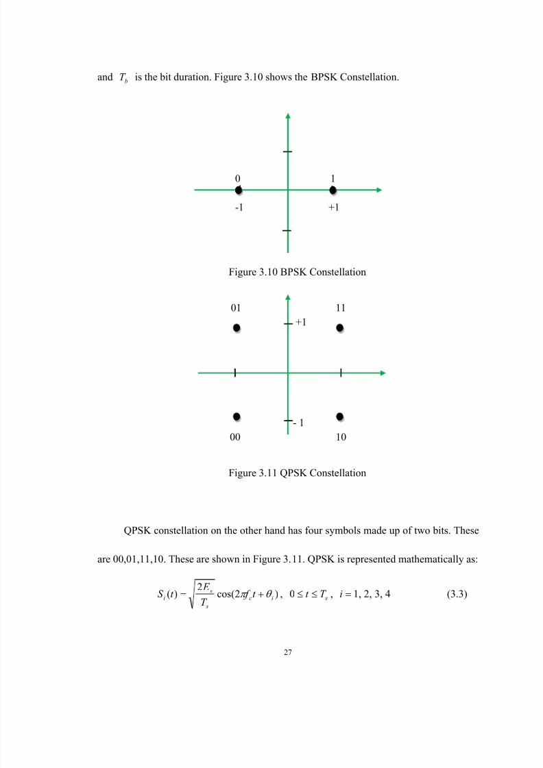
and bT is the bit duration. Figure 3.10 shows the BPSK Constellation.
0 1
-1 +1
Figure 3.10 BPSK Constellation
01 11
+1
- 1
00 10
Figure 3.11 QPSK Constellation
QPSK constellation on the other hand has four symbols made up of two bits. These
are 00,01,11,10. These are shown in Figure 3.11. QPSK is represented mathematically as:
=)(t S i )2cos(2
ic
s
s t f T
E θ π + , sT t ≤≤0 , =i 1, 2, 3, 4 (3.3)

8/8/2019 Oguntade Ayoade Range Estimation for Tactical Radio Waveforms Using Link Budget Analysis
http://slidepdf.com/reader/full/oguntade-ayoade-range-estimation-for-tactical-radio-waveforms-using-link-budget 41/100
28
where4
)12( π θ
−=i
i (3.4)
where s E is the symbol energy, c f is the carrier frequency, iθ is the carrier phase and
sT is the symbol duration.
16 QAM symbols are comprised of four bits. There are 16 different symbols from
0000 to 1111. Its constellation diagram is shown in Figure 3.12.
0010 0110 1110 1010
+3
0011 0111 1111 1011
+1
-3 -1 +1 +3
-1
0001 0101 1101 1001
-3
0000 0100 1100 1000
Figure 3.12 16 QAM Constellation
3.7.4 Data Rate calculation
For the three baseband modulation – BPSK, QPSK and 16 QAM, the data rates used
were calculated based on the bandwidth and the sampling rate. The bandwidth the same
as the sampling rate. The bandwidth of 4 MHz was used for all the modulation schemes.
This equates to a sampling rate s f of 4 MSamples/s.
With a 4 MHz sampling rate, the sampling period becomes s f
1= 0.25 sµ

8/8/2019 Oguntade Ayoade Range Estimation for Tactical Radio Waveforms Using Link Budget Analysis
http://slidepdf.com/reader/full/oguntade-ayoade-range-estimation-for-tactical-radio-waveforms-using-link-budget 42/100
29
For 512 FFT points(samples) used for the WNW, the sampling period bT for the FFT
window becomes:
bT = s s µ µ 12825.0512 =×
Assuming a CP period g T that is ¼ of the FFT window size,
g T = sµ 321284
1=×
Since the symbol duration sT equals the sum of the sampling period bT and the
cyclic prefix period g T , sT becomes,
sT = s s µ µ 160)32128( =+
Assuming BPSK where a symbol contains one bit, the symbol rate then becomes:
Symbol rate = sT s µ 160
11= = 6.25 kbps
The data rate was calculated by the following relationship:
CodeRatel tsperSymbo NumberofBierstaSubcarri NumberofDaSymbolrate Datarate ×××=
Number of Data Subcarriers = 384
Number of Bits per Symbol = 1 (BPSK), 2 (QPSK), 4 (16QAM)
Code rate =2
1,3
1,4
1,8
1and
16
1
8/8/2019 Oguntade Ayoade Range Estimation for Tactical Radio Waveforms Using Link Budget Analysis
http://slidepdf.com/reader/full/oguntade-ayoade-range-estimation-for-tactical-radio-waveforms-using-link-budget 43/100
30
Chapter 4
Channel Impairment Factors This chapter discusses the channel impairment factors that affect radio propagation.
4.1 Propagation Environment
The propagation environment mainly considered for this thesis is the propagation
over ground and sea. The several cases that arise in these considerations are: Ground to
Ground (GTG) and Ground to Ship (GTS). The Ground to Ground cases are further
classified into Ground to Ground open terrain (GTG-O), Ground to Ground Mountain
Blockage (GTG-M) and Ground to Ground Urban (GTG-U) area cases. The sea cases are
the Ground to Ship (GTS) and Ship to Ground (STG) – which are basically the same due
to the law of reciprocity in ground-sea propagation.
4.1.1 Ground to Ground Open Terrain (GTG-O)
The GTG-O is a propagation environment in which the transmitter and receiver have a
clear line of sight and there can be ground reflection of the transmitted signal. The

8/8/2019 Oguntade Ayoade Range Estimation for Tactical Radio Waveforms Using Link Budget Analysis
http://slidepdf.com/reader/full/oguntade-ayoade-range-estimation-for-tactical-radio-waveforms-using-link-budget 44/100
31
transmitter antenna height is denoted as t h , while the receiver antenna height is denoted
as r h . This is shown in Figure 4.1.
Figure 4.1 Ground to Ground Open Terrain (GTG-O)
4.1.2 Ground to Ground Mountain Blockage (GTG-M)
When a Mountain exists between the transmitter and receiver, the propagation
environment that arise is the GTG-M. There is no line of sight between them and the
propagated signal only reaches the receiver by the diffraction of the top of the blockage.
This is can be explained by Huygens construction, which was devised to predict the
successive positions of an advancing wave front. Diffraction is the bending of radio
waves around obstacles that have sharp irregularities (edges). It occurs for waves that
have wavelengths in the order and size of the diffracting objects. Path loss prediction
based on diffraction mechanism used for this environment is the ITU-R single knife edge
diffraction model. This is shown in Figure 4.2. The transmitter and receiver antenna
heights are represented as t h and r h respectively.

8/8/2019 Oguntade Ayoade Range Estimation for Tactical Radio Waveforms Using Link Budget Analysis
http://slidepdf.com/reader/full/oguntade-ayoade-range-estimation-for-tactical-radio-waveforms-using-link-budget 45/100
32
Figure 4.2 Ground to Ground Mountain Blockage (GTG-M)
4.1.3 Ground to Ground Urban (GTG-U)
When propagation takes place in a heavily built-up area where the line of sight
between transmitter and receiver is blocked by buildings and other obstacles, the
environment is modeled as a GTG-U environment. This is shown in Figure 4.3.
Figure 4.3 Ground to Ground Urban Area (GTG-U)
4.1.4 Ship to Ground (STG)
The Ship to Ground propagation models the case in which a communication link is
established between a transmitter located on a ship and receiver located on ground. Both
land and sea contribute a quota to the propagation path. However, the position of the
receiver is different for the three waveforms considered. Due the propagation
characteristic of HFW and VHFW, a ground quota is allowed in the propagation path.

8/8/2019 Oguntade Ayoade Range Estimation for Tactical Radio Waveforms Using Link Budget Analysis
http://slidepdf.com/reader/full/oguntade-ayoade-range-estimation-for-tactical-radio-waveforms-using-link-budget 46/100
33
However, for the WNW, the high frequency of operation (and consequently the high path
loss) requires the propagation path to be restricted to only water – if reasonable
propagation range R is to be achieved. This means that the transmitter (or receiver for the
STG) is placed at the shore to enable the whole propagation to be over the sea. Also, the
placement of the transmitter (or receiver for the STG) at the shore is more practical. The
case of the WNW GTS(STG) is shown in Figure 4.4.
Figure 4.4 WNW Ship to Ground (STG)/Ground to Ship (GTS)
4.1.5 Ground to Ship (GTS)
The Ground to Ship propagation is exactly like the Ship to Ground propagation
discussed above with the position of the transmitter and receiver reversed. The
propagation loss incurred are the same for both the GTS and the STG.
4.1.6 Ship to Ship (STS)
The Ship to Ship propagation models the communication between a transmitter and
receiver both located on the sea. The propagation loss is due to the loss over the sea alone
as there is no ground path involved. It is also assumed that islands that might exist along
the propagation path do not contribute to the loss of the signal.

8/8/2019 Oguntade Ayoade Range Estimation for Tactical Radio Waveforms Using Link Budget Analysis
http://slidepdf.com/reader/full/oguntade-ayoade-range-estimation-for-tactical-radio-waveforms-using-link-budget 47/100
34
4.2 Path Loss Models
The Path loss defined here is solely incurred due to the distance between the
transmitter and the receiver. However, like any other radio communications, It is
frequency dependent because higher frequencies attenuate more than lower ones.
For all the six propagation cases discussed above, Table 4.1 shows the propagation
models that were used in the path loss estimation. Details of these models are discussed
in this section.
Table 4.1 Propagation Model [6]
4.2.1 Hata-Okomura (Hata’s) Model
Hata’s model [7] is a very accurate model when predicting losses in the urban area case.
It predicts the total path loss along a radio propagation link and covers the frequency
range of 150 MHz to 1.5 GHz. Based on Okomura’s work on propagation loss prediction,
Hata constructed an empirical formula to assess propagation losses in urban areas for
systems employing UHF (288 – 910 MHz) and VHF (50 – 250 MHz) land mobile radio
PROPAGATION MODEL
Cases HFW VHFW WNW
GTG-O GRWAVE Plane Earth Hata (Open Area)
GTG-M Lichun Plane Earth+ITU-R Hata (Open Area)+ITU-R
GTG-U Lichun Egli Hata (Urban Area)
STG/GTS MGPP MGPP MGPP
STS GRWAVE MGPP MGPP

8/8/2019 Oguntade Ayoade Range Estimation for Tactical Radio Waveforms Using Link Budget Analysis
http://slidepdf.com/reader/full/oguntade-ayoade-range-estimation-for-tactical-radio-waveforms-using-link-budget 48/100
35
services. The model was based on the propagation loss between systems employing
isotropic antennas, Quasi-smooth terrain and urban propagation loss presented as the
standard formula. For other environments the incorporation of correction factors is
required. Hata’s standard empirical formula, given in equation (4.1), for propagation
loss a function of operating frequency f c, base antenna height hb, mobile antenna height
hm , and transmission distance R. It is mathematically expressed as:
Rhhah f dB L bmbc P 10101010 log)log55.69.44()(log82.13log16.2655.69)( −+−−+= (4.1)
for the following parameter ranges:
f c: 150 – 1500 MHz [Unit: Megahertz]
hb: 30 - 200 m [Unit: Meters]
hm: 1 - 10 m [Unit: Meters]
R: 1 - 20 km [Unit: Meters]
Note that a(hm ) is the correction factor in dB for vehicular station antenna height and is
defined for several varying environments as:
Medium-small city
)8.0log56.1()7.0log1.1()( 1010 −−−= cmcm f h f ha (4.2)
Large City
10.1)54.1(log29.8)(2
10 −= mm hha for f c ≤ 200 MHz (4.3)

8/8/2019 Oguntade Ayoade Range Estimation for Tactical Radio Waveforms Using Link Budget Analysis
http://slidepdf.com/reader/full/oguntade-ayoade-range-estimation-for-tactical-radio-waveforms-using-link-budget 49/100
36
97.4)75.11(log2.3)(2
10 −= mm hha for f c ≥ 400 MHz (4.4)
Suburban Area
The path loss for Suburban Area is taken as a corrected version of the urban area path loss
and is given by:
4.528
log2)(
2
10 −
−= c
P Ps
f Urban LdB L (4.5)
Open Areas
The loss in an open area is again based on urban area losses:
94.40log33.18)(log78.4)( 10
2
10 −+−= cc P O P f f Urban LdB L (4.6)
For a receiver antenna height (hm) of 1.7 m operating in a large city on a frequency f c
of 500 MHz, the antenna correction factor a(hm) of equation 4.4 gives 0.44 dB when
those parameters are plugged into equation 4.4. When the correction factor a(hm) is
plugged into equation 4.1, the estimate the path loss expected at a specific distance R
from the transmitter whose height is hb is generated. Using hb of 1.7 m and a distance of
0.54 km, a path loss (L p) of 124.92 dB was calculated from equation 4.1.
4.2.2 Egli’s Model
Egli’s path loss model [8] is an accurate model for computing the path loss as a
single quantity. This model predicts the path loss as a whole and does not subdivide the loss
into free space loss and other losses. The data used in deriving the model was obtained (by

8/8/2019 Oguntade Ayoade Range Estimation for Tactical Radio Waveforms Using Link Budget Analysis
http://slidepdf.com/reader/full/oguntade-ayoade-range-estimation-for-tactical-radio-waveforms-using-link-budget 50/100
37
the U.S. Federal Communications Commission) from various locations in the United
States including New York City; Washington D.C.; Cleveland and Toledo, Ohio;
Harrisburg, Easton, Reading, Pittsburgh and Scranton, Pennsylvania; Kansas City,
Missouri; Cedar Rapids, Iowa; San Francisco, California; Bridgeport Connecticut;
Nashville, Tennessee; Fort Wayne, Indiana, Richmond and Norfolk, Virginia and Newark,
New Jersey. With regard to UHF (288 MHz – 910 MHz) measurements, 804 miles on 63
different radials are represented in the data. The means of measuring received power was
not the same in all locations. In all, three different techniques were used, continuous mobile
recording sampling every 0.2 miles, spot measurements (properly weighted to be
considered unbiased), and clusters of measurements. For VHF (50 MHz – 250 MHz)
transmissions, approximately 1400 measurements, consisting of continuous data analyzed
over 1 and 2 mile sectors, were also included in the data set. Egli’s model [13] can be
written as:
)(log20log20log40117)( 101010 RT c Egli H H f DdB L −++= (4.7)
where D is the transmission distance in miles, f c is the transmission carrier frequency in
MHz, H T is the transmitting antenna height above ground level in feet and H R is receiver
antenna above ground level in feet.
4.2.3 GRWAVE Model
GRWAVE [9][10] is a computer program and has been used by ITU-R to produce the

8/8/2019 Oguntade Ayoade Range Estimation for Tactical Radio Waveforms Using Link Budget Analysis
http://slidepdf.com/reader/full/oguntade-ayoade-range-estimation-for-tactical-radio-waveforms-using-link-budget 51/100
38
series of CCIR (reference) curves which show how vertically polarized electrical field
strength varies as a function of range, ground type, and frequency (10 KHz to 30 MHz).
This computer program was developed by for the prediction of ground wave propagation
path loss at the HF frequency band. The program takes as inputs the Frequency of
transmission, Effective radiated power, Polarization type (Vertical or Horizontal), the
Ratio of the effective earth radius to the actual earth radius, Ground conductivity in S/M,
Ground dielectric constant relative to free space, Antenna heights and the Distance
between transmitter and receiver. In applying the GRWAVE path loss prediction program
to system planning purposes, it is essential to have a clear understanding of the reference
radiator used in their calculation. The transmitting antenna is a Hertzian vertical dipole
with a current length product (dipole moment) of π
λ
2
5, where λ is the wavelength of
the frequency used. The GRWAVE model assumes that the radio wave propagates over
a smooth homogeneous spherical earth for frequencies between 0.03 to 30 MHz and the
antenna heights of zero to 20 km. Link length from 1 to 10,000 km. The conductivity and
permittivity values used for the GRWAVE are shown in Table 4.2. Also Figure 4.5 shows
the screenshot of the GRWAVE for the HFW and the values of the parameters used.
Table 4.2 Conductivity and permittivity values for Land and Sea [6].
Ground Type Conductivityσ (S/m)
Permittivity
r ε
Sea 5 70
Land 0.01 15

8/8/2019 Oguntade Ayoade Range Estimation for Tactical Radio Waveforms Using Link Budget Analysis
http://slidepdf.com/reader/full/oguntade-ayoade-range-estimation-for-tactical-radio-waveforms-using-link-budget 52/100
39
Figure 4.5 Screenshot for the GRWAVE model as used for HFW
4.2.4 Millington’s Model
When the propagation path is inhomogeneous, special models like Millington’s
[11] are needed for estimating the path loss. Eckersley intuitively proposed (shown in
Figure 4.6a) using sections of the surfaced wave attenuation curves (like the ones by the
ITU-R) appropriate for the radio frequency and terrain type. That is the loss curves for
each terrain type are patched together in a piece-wise fashion to yield an overall
prediction; however, this model does not agree well with experiment. Moreover,
Eckersley’s method does not yield the same prediction value when transmitting from
transmitter (T) to receiver (R) as when transmitting from R to T. Millington, argued that
if T is well removed from point X (as shown in Figure 4.6), then the attenuation rate will
be dictated largely by terrain type 1 (ground with different conductivity and permittivity

8/8/2019 Oguntade Ayoade Range Estimation for Tactical Radio Waveforms Using Link Budget Analysis
http://slidepdf.com/reader/full/oguntade-ayoade-range-estimation-for-tactical-radio-waveforms-using-link-budget 53/100
40
value from ground type 2); likewise, if the transmission is launched from R and is well
removed from X, then the loss is largely governed by ground type 2 (ground with
different conductivity and permittivity value from ground type 1). Moreover, he argued
that reciprocity between bidirectional transmissions must be enforced. Thus, Millington
proposed applying Eckersley’s method in the T-R (forward) direction and the R-T
(reverse) direction. These two values are then averaged to yield the overall loss as shown
in Figure 4.6b. Millington’s method has been implemented in a Matlab as Millington
Propagation Predictor (MGPP) by [12][13].
(a) (b)
Figure 4.6 (a) Eckersley’s prediction method (b) Millington’s prediction method [10].
4.2.5 Lichun Model
Lichun model [14] was derived based on the experimental data collected at HF frequency
from 1993 through 1997 in Beijing, China. This model introduces the inclusion of three
building-complex parameters br , sr and er , and a new height-gain factor, hG . The

8/8/2019 Oguntade Ayoade Range Estimation for Tactical Radio Waveforms Using Link Budget Analysis
http://slidepdf.com/reader/full/oguntade-ayoade-range-estimation-for-tactical-radio-waveforms-using-link-budget 54/100
41
building-complex parameters represents the impact of buildings on ground waves in
urban areas and their values were selected based on our urban environment. The values
used were: 0.26, 0.5, 0.05 for br , sr and er respectively.
The equation for the estimated path loss by Lichun model is written below:
he sbd g f G L L L L L LdB L −+++++=)( (4.8)
where:
Table 4.3 Lichun Model Parameters
Loss Component Equation Unit1 Free Space Loss Lf R f 1010 log20log204.32 ++
dB
2 Ground loss Lg A10log20− dB
3 Propagation Distance loss Ld R10log16dB
4 Building loss Lb )1(log95 10 br +
dB
5 Sight loss Ls )1(log80 10 sr +
dB
6 Environment loss Le )1(log125 10 er +
dB
7 New height gain factor Gh )(log)02.01(20 10 r t hh R ++
dB
The equation parameters are given as:
A =)(),,(2
101
3
m R f c β σ ϕ
−×, (4.9)
σλ
β β σ ϕ
cos1075.1),,( 4 c
c
f f −×= (4.10)

8/8/2019 Oguntade Ayoade Range Estimation for Tactical Radio Waveforms Using Link Budget Analysis
http://slidepdf.com/reader/full/oguntade-ayoade-range-estimation-for-tactical-radio-waveforms-using-link-budget 55/100
42
σ
ε β
4108.1
)1(arctan×
+= c f
(4.11)
where
R: Link Length (km)
ht : Height of transmitting antenna
hr : Height of receiving antenna
c f : Operating frequency (MHz)
A : Attenuation factor of the ground
λ : Wavelength of the propagating wave
β : Phase constant
and the ground constants are:
ε = 15 and σ = 3101 −× S/m (Weather is fine and cloudy)
Lichun model has been used to estimate the Path Loss in Urban and Mountain blockage
cases of the HF-AM propagation in the research work. The results show that the Loss
experienced in the Urban area propagation is more than the Loss incurred in the
Mountain blockage case since a single mountain was considered.
4.2.6 ITU-R Model
A mountain blockage scenario is the one with a hill or mountain in the signal
propagation path as shown in Figure 4.2. The mechanism that takes place in the

8/8/2019 Oguntade Ayoade Range Estimation for Tactical Radio Waveforms Using Link Budget Analysis
http://slidepdf.com/reader/full/oguntade-ayoade-range-estimation-for-tactical-radio-waveforms-using-link-budget 56/100
43
propagation of radio waves when there is a blockage between transmitter and receiver is
diffraction. Diffraction is the bending of radio waves around obstacles that have sharp
irregularities (edges). It occurs for waves that have wavelengths in the order and size of
the diffracting objects. Path loss prediction based on diffraction mechanism can be done
in two ways. These are: Smooth spherical earth diffraction and the Knife edge diffraction.
The smooth spherical earth diffraction is applicable in a scenario where the receiver is
located beyond the line of sight of the transmitter and there are no mountains in between.
A knife edge diffraction results when the LOS between a transmitter and receiver is
obstructed by a hill or mountain. A transmitted signal still reaches the receiver via
diffraction off the top on the obstacle in the path of the transmitter and the receiver. This
can be explained by Huygens construction, which was devised to predict the successive
positions of an advancing wave front.
If the hills are two or more, multiple knife edge diffraction occurs. It is also
noteworthy to say that the presence of obstacle sometimes leads to increased signal
strength at the receiver which is known as obstacle gain. This happens when the multiple
diffraction path with high loss is transformed into single edge diffraction path with less
loss [15].
The ITU-R model is one of several models (including Epstein – Peterson,
Deygout, Edward–Durkins and Blomquist - Ladell) which estimate diffraction loss due to
terrain blockage. Investigations have shown that the ITU-R model produced the result

8/8/2019 Oguntade Ayoade Range Estimation for Tactical Radio Waveforms Using Link Budget Analysis
http://slidepdf.com/reader/full/oguntade-ayoade-range-estimation-for-tactical-radio-waveforms-using-link-budget 57/100
44
closest to the empirical measurements [10]. In this model, the diffraction parameter v is a
dimensionless parameter and it is given by the formula:
+=
21
112d d
hvλ
(4.12)
Where λ is the wavelength of the signal and the parameters h, d 1 and d 2 are as shown in
Figure 4.2. Also, h is the height of the diffraction above the LOS between the transmitter
and receiver. The diffraction loss can be given as:
J (v) = 6.9 + 20log ( 12 +v + v ) (dB) (4.13)
This diffraction loss is added to the path loss model (because both the transmitter and
receiver antenna heights are low and close to the ground) applicable to the frequency
range of interest.
4.2.7 Plane Earth Model
The plane earth loss is frequency independent. It has been found out that the loss
figure gotten from the calculation of the plane earth loss is not as high as that of
measured data so a clutter factor is added to the calculated figure to compensate for the
dB figure difference. It has be found to hold for particular distances and for horizontal

8/8/2019 Oguntade Ayoade Range Estimation for Tactical Radio Waveforms Using Link Budget Analysis
http://slidepdf.com/reader/full/oguntade-ayoade-range-estimation-for-tactical-radio-waveforms-using-link-budget 58/100
45
polarization [14]. The plane earth model formula is given as:
)(log20log406.144)( 1010 r t PE hhd dB L −+= (4.14)
where d is distance between transmitting dipole antennas in miles, ht is the height of
transmitting antenna (ft), and hr is the height of receiving antenna (ft).
4.3 Shadowing – Long term fading
If a transmitter is placed at the center of an imaginary circle as shown in Figure 4.7,
the amount of signal power received at different points on its circumference by moving a
receiver round it does not necessarily have to be the same even though the points are
equidistant from the transmitter. Obstructions might be present between the transmitter
and the receiver at some points on the circumference while a line of sight might exists on
others. Unlike path loss which is distance dependent, Shadowing statistically describes
this effect and has been found to be a log-normally distributed random process.
Figure 4.7 Shadowing variation over different paths [16].

8/8/2019 Oguntade Ayoade Range Estimation for Tactical Radio Waveforms Using Link Budget Analysis
http://slidepdf.com/reader/full/oguntade-ayoade-range-estimation-for-tactical-radio-waveforms-using-link-budget 59/100
46
4.4 Multipath - Short term fading
When a transmitted signal reaches a receiver via several paths, several copies of it
appear at the receiver with several delays and gains. The time delay results in phase shifts
in the signal copies and results in the their destructive re-combination. This makes the
original signal to fade. Rayleigh and Rician are some of the statistical methods for
characterizing a multipath channel.
4.4.1 Rayleigh Fading Distribution
Rayleigh distribution are useful in the characterization of a wireless channel where a
line of sight (dominant path) does not exist. The received signal is only composed of
several multipath reflected signals. The signal components are also assumed to be
independent (uncorrelated), identical in amplitude and have random phases that are
uniformly distributed between 0 and 2π. The Probability Density Function (pdf) of the
Rayleigh distribution is given by:
)0(
)0(
<
≤
r
r
(4.15)
Where r is the signal envelope, σ is the Root Mean Square (RMS) value of the
received voltage signal, and 2σ is the time-average power of the received signal. σ is
the spread of the distribution.
−
=
0
2exp
)( 2
2
2σ σ
r r
r p

8/8/2019 Oguntade Ayoade Range Estimation for Tactical Radio Waveforms Using Link Budget Analysis
http://slidepdf.com/reader/full/oguntade-ayoade-range-estimation-for-tactical-radio-waveforms-using-link-budget 60/100
47
4.4.2 Rician Fading Distribution
When a dominant Line of Sight (LOS) component exists between the transmitter and
receiver, the channel is said to follow a Rician distribution and the LOS component is
called the specular component. As the amplitude of the specular component approaches
zero, the Rician pdf approaches a Rayleigh pdf [4]. The Rician pdf is given by,
)0(
)0,0(
<
≥≥
r
r V
(4.16)
where r is the signal envelope, V is the amplitude of the specular component of the
received signal and σ is the Root Mean Square (RMS) value of the received voltage
signal (the spread of the distribution). As V tends to zero, the pdf approaches a
Rayleigh pdf. I 0( z ) is the modified Bessel function of the first kind with order zero.
The Rician K -factor is defined as the ratio of signal power in dominant component
over the (local-mean) scattered components’ power which is
K (dB)=2
2
102
log10σ
V . dB (4.17)
When K>>>1, the Rician distribution tends towards the Gaussian distribution about
the mean, which characterizes a non-fading channel.
+−
=0
)(2
)(exp
)( 22
22
2 σ σ σ
rV I
V r r
r p O

8/8/2019 Oguntade Ayoade Range Estimation for Tactical Radio Waveforms Using Link Budget Analysis
http://slidepdf.com/reader/full/oguntade-ayoade-range-estimation-for-tactical-radio-waveforms-using-link-budget 61/100
48
4.4.3 Nakagami-m Fading Distribution
The sum of multiple independent and identically distributed (i.i.d.) Rayleigh-fading
signals have Nakagami-m distributed signal amplitude. Nakagami-m fading distribution
is a very important distribution due to its ease of manipulation and wide range of
applicability [17]. It also has been found to yield a satisfactory fit with measured fading
data over a wide range of frequency bands [18]. The Nakagami-m probability density
function of a signal’s envelope r is given by the formula,
Ω−−
ΩΓ=
2
12
2
)(
2)(
mr m er
m
mr p
(4.18)
,0≥r ,5.0≥m ,0≥Ω
where Γ(.) is the gamma function, m = E2
(x2
)/var(x2
) is the shape factor which
determines the severity of fading, and = E(x2) is the mean square value of the
distribution. The Nakagami fading turns to a Rayleigh fading at m=1 and becomes a
one-sided Gaussian distribution for m = 0.5. The distribution becomes an impulse
(Dirac-delta function) when m = ∞, which implies an AWGN channel with no fading.

8/8/2019 Oguntade Ayoade Range Estimation for Tactical Radio Waveforms Using Link Budget Analysis
http://slidepdf.com/reader/full/oguntade-ayoade-range-estimation-for-tactical-radio-waveforms-using-link-budget 62/100
49
4.5 Other Fading Issues
4.5.1 Frequency Flat and Frequency Selective Channels
When fading affects all the spectral components of a transmitted signal in a similar
manner, the fading is said to be frequency flat. This is typical of narrowband systems. On
the other hand, when spectral components of a transmitted signal are affected by different
amplitude gains and phase shifts, the fading is said to be frequency selective – which is
characteristic of wideband systems like the OFDM.
4.5.2 Doppler Shift
When a transmitter and receiver are moving relative to one another, the frequency of
the received signal will deviate from that of the signal which was transmitted. When the
radios move towards each other, the received signal is higher than that of the transmitted
signal; the opposite is becomes true when they are moving further apart. The received
frequency is then given by:
d cr f f f ±= (4.19)
(shift) is governed by: where f d is the Doppler frequency (or Doppler shift) and f c is the
transmitting source carrier frequency. The Doppler frequency is defined as,
θ λ
cosv
f d = (4.20)
where v is the velocity of light in meters per second, λ is the carrier wavelength in meters,
and Ө is the angle between the transmitting source and the receiver’s direction of travel in

8/8/2019 Oguntade Ayoade Range Estimation for Tactical Radio Waveforms Using Link Budget Analysis
http://slidepdf.com/reader/full/oguntade-ayoade-range-estimation-for-tactical-radio-waveforms-using-link-budget 63/100
50
degrees.
4.5.3 Coherence Time and Doppler spread
Doppler spread and coherence time are parameters which describe the time varying
nature of the channel in a small-scale region. Doppler spread, Bd , is a metric used to define
the spectral broadening caused by the time rate of change of the mobile radio channel. It is
defined as the range of frequencies over which the received Doppler spectrum is essentially
non-zero. If a sinusoid of frequency f c is transmitted, the receiver will receive frequency
components in the range of f c ± f d , where f d is the Doppler frequency shift. Note that if the
baseband signal is significantly larger than Bd , then the effects of Doppler spread will be
negligible at the receiver.
Coherence time is the time dual of the Doppler spread and describes the time varying
nature of the frequency dispersion of the channel in the time domain. The coherence time
and Doppler spread are inversely proportional to each other,
d
C f
T 1= (4.21)

8/8/2019 Oguntade Ayoade Range Estimation for Tactical Radio Waveforms Using Link Budget Analysis
http://slidepdf.com/reader/full/oguntade-ayoade-range-estimation-for-tactical-radio-waveforms-using-link-budget 64/100
51
Chapter 5
Link Budget Analysis
5.1 Link Budget
Link Budget Analysis is a very important tool in estimating the propagation range
that can be achieved by a transmitter with a specified power. If the propagation
environment is well known, this is a very good way of predicting the performance of a
radio equipment before it is manufactured. The link budget is achieved by taking account
of all the gains and losses in the propagation path. The net of the gains and losses allows
for a margin that would ensure that a receiver can still pick up the transmitter’s signal
even when the channel experiences the worst level of is attenuation. This chapter
describes all the necessary parameters for performing the link budget for the three tactical
waveform of interest to us.
5.2 Equipment Types
Two separate types of equipment types have been used for this thesis. They are the

8/8/2019 Oguntade Ayoade Range Estimation for Tactical Radio Waveforms Using Link Budget Analysis
http://slidepdf.com/reader/full/oguntade-ayoade-range-estimation-for-tactical-radio-waveforms-using-link-budget 65/100
52
manpack equipment and the vehicle mounted equipment.
5.2.1 Manpack Equipment
The manpack equipment is carried as back packs by its users. It has a smaller form factor
when compared to the vehicle mounted equipment and operates on less power.
5.2.2 Vehicle Equipment
The vehicle-mounted equipment is installed in vehicles where further power
amplification is provided so as to enhance the propagation range of the signal. The
antenna height (in meters), antenna gain (in decibel isotropic - dBi) and the transmitter
power (in watts) used for the three waveforms – HFW, VHFW and the WNW - are
considered are shown in Table 5.1. The dBi unit of the antenna gain is a measure which
stipulates the gain of an antenna relative to an isotropic radiator. An Isotropic radio is a
point source in which signal is radiated from the point to form a sphere. That means
radiation is equal in all directions. For example an antenna with a 0 dBi gain has the same
signal propagation ability as an isotropic radiator while an antenna -15 dBi gain is 15dB
‘weaker’ in propagation ability when compared to an isotropic radiator.

8/8/2019 Oguntade Ayoade Range Estimation for Tactical Radio Waveforms Using Link Budget Analysis
http://slidepdf.com/reader/full/oguntade-ayoade-range-estimation-for-tactical-radio-waveforms-using-link-budget 66/100
53
Table 5.1 Parameters for Manpack and Vehicle Equipment
5.3 Link Budget Parameters
To perform the link budget for the waveforms of our communications link, several
parameters are needed. These include the transmitter power, power back-off, carrier
center frequency, the height and the gain of the antenna, the thermal noise present in the
bandwidth of the signal, the noise figure of the receiver and the acceptable link margin to
the system designer.
5.3.1 Transmitter Power
The transmitter power used for this work are based on the two type of equipment
used. These are manpack and vehicle mounted equipment. The Manpack equipment
operates on 5 W of power while the vehicle mounted equipment operates on 50 W for
both the VHFW and the WNW. The HFW waveform uses two power levels – 20 W and
Antenna Height (m) Tx/R x
HFW VHFW WNW
Manpack 2.52 1.70 1.70
Vehicle 7.30 2.80 2.80
Antenna Gain (dBi)
HFW VHFW WNW
Manpack -15 dBi -15 dBi 0 dBi
Vehicle -15 dBi -6 dBi 0 dBi
Tx Power (Watts)
HFW VHFW WNW
Manpack 20 W 5 W 5 W
Vehicle 100 W 50 W 50 W

8/8/2019 Oguntade Ayoade Range Estimation for Tactical Radio Waveforms Using Link Budget Analysis
http://slidepdf.com/reader/full/oguntade-ayoade-range-estimation-for-tactical-radio-waveforms-using-link-budget 67/100
54
100W. All these were shown in Table 5.1.
5.3.2 Power Back-Off
When the power amplifier of a communication system is being pushed towards its
non-linear region (saturation), the power of the amplifier needs to be moved back to its
linear operating region. This process is called Power Back-Off. This was done to our
manpack and vehicle mounted equipment. The amount of power back off was 5.5 dB.
5.3.3 Center frequency
The center frequency used for the HFW is 27 MHz while the one used for the VHFW
is 60 MHz. The WNW uses a 500 MHz center frequency. The center frequency is
measured in MHz. The detection bandwidth used with these center frequencies of 27, 60
and 500 MHz are 4 KHz, 25 KHz, and 4 MHz respectively.
5.3.4 Antenna Height
The antenna height plays a very important role in the propagation range of a
transmitted signal. The antenna height used for the manpack equipment was 1.7 m while
the one for the vehicle mounted equipment was 2.8 m. The antenna height is measured in
meters.

8/8/2019 Oguntade Ayoade Range Estimation for Tactical Radio Waveforms Using Link Budget Analysis
http://slidepdf.com/reader/full/oguntade-ayoade-range-estimation-for-tactical-radio-waveforms-using-link-budget 68/100
55
5.3.5 Antenna Gain
The antenna gain used in this thesis is the one relative to an isotropic radiator. This is
specified in dBi. The antenna gain value that was used for the manpack equipment for the
HFW, VHFW and WNW were -15 dBi, -15 dBi and 0 dBi respectively. For the Vehicle
mounted equipment, antenna gains of -15 dBi, -6 dBi and 0 dBi were used for the HFW,
VHFW and WNW.
5.3.6 Thermal Noise Power
Apart from Additive White Gaussian Noise encountered in the channel, noise is
generated by thermal agitation of electrons in the electronic components in receivers.
This inherent Noise is called Thermal Noise. The thermal noise power, P , in watts, is
given by P = k T B, where k is Boltzmann's constant in joules per kelvin, T is the
conductor temperature in kelvin, and B is the bandwidth in Hertz. Thermal noise power,
per Hertz, is equal throughout the frequency spectrum, depending only on k and T .
5.3.7 Noise Figure
Noise Figure is a parameter that specifies the performance of radio receivers. It is
measured in dB. It is a measure of how much a receiver degrades the signal at its input as
compared to its output. It can also be described as the decibel difference in the noise
output of an actual receiver to the noise output of an ideal receiver (one which introduces

8/8/2019 Oguntade Ayoade Range Estimation for Tactical Radio Waveforms Using Link Budget Analysis
http://slidepdf.com/reader/full/oguntade-ayoade-range-estimation-for-tactical-radio-waveforms-using-link-budget 69/100
56
no thermal noise) under the same gain, bandwidth, and noise temperature conditions. A
Noise Figure of 6 dB was assumed for the receiver to perform the Link Budget Analyses.
5.3.8 Link Margin
To provide for the contingencies like fading, increase the thermal noise generated by
the receiver (due to its operation under harsh temperature conditions), a link margin is
necessary for the Link Budget. The amount of Link margin to be provided for depends on
the level of degradation that is expected. The LBAs in this thesis provide a link margin of
0.5 dB for all the cases considered. The equation that define the Link margin is given as:
Link margin (dB) = Receiver Sensitivity – Power Left at the Receiver Input (5.1)
where,
(1) Receiver sensitivity = kTB + Noise Figure + SNR (dBm) (5.2)
BkT kTB 10log10+= (dB) (5.3)
Thermal Noise Density: 174−=kT (dB/Hz)
Boltzmann's constant: k = 201038.1 −
× (dBm/K)
Receiver system noise temperature: T (Kelvin).
Detection Bandwidth: B (Hertz).
Noise Figure: NF (dB)
(2) Power Left at the Receiver Input (dBm) = imprxrxtxtxbo x LG A LG A P T −+−−+−−

8/8/2019 Oguntade Ayoade Range Estimation for Tactical Radio Waveforms Using Link Budget Analysis
http://slidepdf.com/reader/full/oguntade-ayoade-range-estimation-for-tactical-radio-waveforms-using-link-budget 70/100
57
where xT is the transmitter power, bo P is the power back-off, tx A is the transmitter
feedline loss, txG is the transmitter antenna gain, L is the Path loss, rx A is the
receiver feedline loss, rxG is the receiver antenna gain, and imp L is the implementation
loss.
5.4 Sample Link Budget Analysis
To show how all the parameters work together in performing a Link Budget Analysis,
A sample LBA is shown here. The LBA has been divided into three segments which
shows the three different stages of the radio system: Transmitter, Channel and Receiver.
The transmitter part shows the transmitter parameters and the values used at different data
rates. The channel part shows the link length that is possible under the specified channel
conditions – the path loss, and the operating frequency. The receiver part shows the effect
of the detection bandwidth and the thermal noise power generated by it. This sample LBA
shows the result of LBA performed for a 5 W WNW radio equipment operating in a
GTG-Open propagation environment.

8/8/2019 Oguntade Ayoade Range Estimation for Tactical Radio Waveforms Using Link Budget Analysis
http://slidepdf.com/reader/full/oguntade-ayoade-range-estimation-for-tactical-radio-waveforms-using-link-budget 71/100
58
A. TRANSMITTER
Data Rates
Description Quantity Unit 120kbps 240kbps 480kbps 960kbps 1.92Mbps 2.5Mbps
Transmitter Power Tx dBm 37.00 37.00 37.00 37.00 37.00 37.00
Power Back-off Pbo dBm 0.00 5.50 5.50 5.50 5.50 5.50
Transmitter Antenna Gain Gtx dB 0.00 0.00 0.00 0.00 0.00 0.00
Transmitter Feedline Loss A tx dB 0.00 0.00 0.00 0.00 0.00 0.00
Transmitter Antenna Height hb m 1.70 1.70 1.70 1.70 1.70 1.70
B. CHANNEL
Link Length R Km 3.41 2.69 2.30 1.76 1.42 0.98
Frequency f c MHz 250.00 250.00 250.00 250.00 250.00 250.00
Path Loss (Hata, Open Area) L dB 127.39 122.92 119.97 114.92 110.92 103.97
C. RECEIVER
Receiver Antenna Gain Grx dB 0.00 0.00 0.00 0.00 0.00 0.00
Receiver Feedline Loss A rx dB 0.00 0.00 0.00 0.00 0.00 0.00
Receiver Antenna Height hm m 1.70 1.70 1.70 1.70 1.70 1.70
Thermal Noise Density kT dBm/Hz -174.00 -174.00 -174.00 -174.00 -174.00 -174.00
Detection Bandwidth B kHz 4000.00 4000.00 4000.00 4000.00 4000.00 4000.00
Thermal Noise Power across B kTB dBm -107.98 -107.98 -107.98 -107.98 -107.98 -107.98
Noise Figure NF dB 8.00 6.00 6.00 6.00 6.00 6.00
Implementation Loss L(imp) dB 0.00 0.00 0.00 0.00 0.00 0.00
Required S/N Ratio@BER 10-5 Eb /No dB 9.00 10.00 13.00 18.00 22.00 29.00
Power Left at Receiver Input PWR rx dBm -90.39 -91.42 -88.47 -83.42 -79.42 -72.47
Receiver Sensitivity PWR sen dBm -90.98 -91.98 -88.98 -83.98 -79.98 -72.98
Link Budget Margin Margin dB 0.59 0.56 0.51 0.56 0.56 0.51
Figure 5.1 Sample Link Budget Analysis
5.4.1 Sample LBA calculation for GTG-O
To show the LBA calculations, the link parameters shown in Table 5.1 were subsumed
under two main categories: Losses and Gains. This section shows how we arrived at the

8/8/2019 Oguntade Ayoade Range Estimation for Tactical Radio Waveforms Using Link Budget Analysis
http://slidepdf.com/reader/full/oguntade-ayoade-range-estimation-for-tactical-radio-waveforms-using-link-budget 72/100
59
link margin shown in figure 5.1 for the 960 kbps data rate, in the GTG-O case. The link
margin has been obtained by taking the difference between the gains and the losses in the
communication link. The details are shown below:
A. Gains
1. Transmitter Power = 37 dBm, 2. Transmitter Antenna Gain = 0 dBi, 3.
Receiver Antenna Gain = 0 dBi. This makes the sum of all the gain in the
system to be 37 dB.
B. Path Loss
1. Transmitter Antenna Height = 1.7 m, 2. Receiver Antenna Height = 1.7 m,
3. Link Length = 1.76 km, 4. Frequency = 500 MHz
Considering the Hata open area path loss which uses the formula:
Rhhah f dB L bmbc P 10101010 log)log55.69.44()(log82.13log16.2655.69)( −+−−+=
where )8.0log56.1()7.0log1.1()( 1010 −−−= cmcm f h f ha ,
The path loss calculated by substituting all the four parameters is 114.92 dB.
C. Other Loses
1. Power Back-off = 5.5 dB, 2. Transmitter Feedline Loss = 0 dB,
3.Receiver Feedline Loss = 0 dB, 4. Implement Loss = 0 dB.
The sum of the other losses is 5.5 dB.

8/8/2019 Oguntade Ayoade Range Estimation for Tactical Radio Waveforms Using Link Budget Analysis
http://slidepdf.com/reader/full/oguntade-ayoade-range-estimation-for-tactical-radio-waveforms-using-link-budget 73/100
60
. Thermal Noise Power
1. Thermal Noise Density (kT)= -174 dBm/Hz ,
2. Detection Bandwidth = 4 MHz.
The thermal noise power across 4 MHz (4,000,000 Hz) becomes
)000,000,4(log10174 10+−=kTB (dB)
= -174 +66.02 = - 107.98 dB
E. Noise Figure (NF) = 6 dB
We have assumed a receiver of 6 dB noise figure.
F. Required S/N = 18 dB
G. Power Left at Receiver Input = A - B – C
= 37 – 114.92 – 5.5 = - 83.42
H. Receiver Sensitivity = D + E + F
= -107.98+6+18 = - 83.98 dB
Then, Overall Link Margin = G – H
= -83.42 – (- 83.98) = 0.56 dB
For the GTG-M, GTS and other cases, the same procedure applies. The only difference
will be parameter B – which is the path loss estimation.

8/8/2019 Oguntade Ayoade Range Estimation for Tactical Radio Waveforms Using Link Budget Analysis
http://slidepdf.com/reader/full/oguntade-ayoade-range-estimation-for-tactical-radio-waveforms-using-link-budget 74/100
61
Chapter 6
Discussion of Results
This Chapter discusses the results obtained by performing LBA for the three
waveforms under five propagation environments: GTG-O, GTG-M, GTG-U, STG/GTS
and STS. Tables 6.1 through 6.3 summarizes the range estimated for all the waveforms.
The results are shown for Tx power of 20 W and 100 W for the HFW, and 5 W and 50 W
for both the VHFW and the WNW.
The maximum and minimum propagation range shown in Tables 6.1 through 6.3 are
for the minimum and maximum data rates respectively. The lowest data rates gave the
maximum range shown while the highest data rates gave the minimum range shown.
Table 6.1 Estimated range for all the HFW cases
HFW 27 MHz Detection Bandwidth, B = 3 kHz
Tx Power (20 W) (100 W)
Range(km) Max Min Max Min
GTG-O 20.0 7.0 36.5 13.5
GTG-M 11.8 4.76 32.0 10.8
GTG-U 4.92 2.14 11.29 4.44
STG/GTS 68.0 25.0 94.6 42.5
STS 158 95 180 115

8/8/2019 Oguntade Ayoade Range Estimation for Tactical Radio Waveforms Using Link Budget Analysis
http://slidepdf.com/reader/full/oguntade-ayoade-range-estimation-for-tactical-radio-waveforms-using-link-budget 75/100
62
Table 6.2 Estimated range for the VHFW cases
VHFW 60 MHz Detection Bandwidth, B = 25 kHz
Tx Power (5 W) (50 W)
Mode Fixed Hopping Fixed Hopping
Range(km) Max Min Max Min Max Min Max Min
GTG-O 2.82 0.82 2.75 0.75 23.4 6.80 25.5 6.22
GTG-M 0.20 0.04 0.19 0.03 3.37 0.64 3.24 0.58
GTG-U 1.73 0.50 1.68 0.46 14.3 4.15 13.9 3.8
STG/GTS 12.0 3.5 11.9 3.00 45.5 17.5 45.0 16.0
STS 26.5 9.50 26.0 9.00 80.0 35.0 78.5 33.0
Table 6.3 Estimated range for the WNW cases
WNW 500 MHz Detection Bandwidth, B = 4 MHz
Tx Power (5 W) (50 W)
Mode Long Frame Short Frame Long Frame Short Frame
Range(km) Max Min Max Min Max Min Max Min
GTG-O 2.49 0.72 1.91 1.22 6.00 1.66 4.57 2.87
GTG-M 0.12 0.02 0.08 0.05 0.33 0.06 0.23 0.12
GTG-U 0.62 0.18 0.47 0.30 1.38 0.38 1.05 0.65
STG/GTS/STS 1.70 0.40 1.20 0.70 4.50 1.10 3.40 2.00
6.1 HFW Propagation Range
This section discusses the propagation range of the HFW under different propagation
environment. They are the GTG-O, GTG-M, GTG-U, STG/GTS, and STS. Table 6.1
serves as reference for the HFW and the propagation environments.
6.1.1 HFW GTG-O
The GRWAVE program was used to model for estimating path loss for the case of
HFW GTG-O. The five different data rates used are of 75 bps, 150 bps, 300 bps, 600 bps,

8/8/2019 Oguntade Ayoade Range Estimation for Tactical Radio Waveforms Using Link Budget Analysis
http://slidepdf.com/reader/full/oguntade-ayoade-range-estimation-for-tactical-radio-waveforms-using-link-budget 76/100
63
1.2 kbps, 2.4 kbps for lower data rate assessment. The transmitter and receiver antenna
gains used for the LBA is -15 dBi. The link margin between 0.5 and 1 dB targeted in the
LBA to estimate the transmission range and the results are shown below in Table 6.4.
Table 6.4 Summary of LBA for HFW GTG-O case.
Distance (km)
Manpack (20 W) Vehicle (100 W)
Maximum Minimum Maximum Minimum
20.0 7.0 36.5 13.5
As can be seen from the Table, the Manpack equipment with Tx power 20 W can achieve
link distance from 7 km to 20 km, while the vehicle with Tx power 100 W can achieve link
distance from 13.5 km to 36.5 km. For better transmission range, it is recommended that
high gain antennas be used.
6.1.2 HFW GTG-M
This is the last case of the HFW GTG cases. The data rates used herein were
comprised of 75 bps, 150 bps, 300 bps, 600 bps, 1.2 kbps, and 2.4 kbps for LBA. Just like
GTG-U case, it also uses Lichun model to estimate the path loss in the mountain
blockage scenario. The Lichun model (as used in this case) assumes a single obstruction
in the propagation path between transmitter and receiver. The use of Lichun model for
this case neglects the sight loss (Ls) and the environment loss (Le) because they do not

8/8/2019 Oguntade Ayoade Range Estimation for Tactical Radio Waveforms Using Link Budget Analysis
http://slidepdf.com/reader/full/oguntade-ayoade-range-estimation-for-tactical-radio-waveforms-using-link-budget 77/100
64
contribute to the path loss in the case. The propagation distances that resulted from the
LBA are shown in Table 6.5.
Table 6.5 Summary of LBA for HFW GTG-M case.
Distance (km)
Manpack (20 W) Vehicle (100 W)
Maximum Minimum Maximum Minimum
11.8 4.76 32.0 10.8
It can be observed from the Table that the Manpack equipment with Tx power 20 W can
achieve link distance from 4.76 km to 11.8 km, while the vehicle with Tx power 100 W can
achieve link distance from 10.8 km to 32.0 km. Comparing the results of case GTG-O and
GTG-U, it is observed that the mountain blockage case produced a better range of coverage
than the urban case. This is because propagation in an urban area is attenuated more than
the mountain blockage case due to the presence of many buildings in the urban area case.
6.1.3 HFW GTG-U
This is a case for HF propagation in urban areas. Lichun Model was used to
model the path loss in this case. This model is based on empirical data collected in urban
areas of China. The path loss generated by Lichun model is made up of the sums all the
losses encountered in propagating a radio signal from transmitter to receiver and the gain
produced by the height of the Tx and Rx antennas above ground. The losses are: Free
Space Loss, Ground loss, Propagation Distance loss, Building loss, Sight loss,

8/8/2019 Oguntade Ayoade Range Estimation for Tactical Radio Waveforms Using Link Budget Analysis
http://slidepdf.com/reader/full/oguntade-ayoade-range-estimation-for-tactical-radio-waveforms-using-link-budget 78/100
65
Environment loss. The antenna gain factor is called the new height gain factor. The LBA
has been done based on link margin of 0.5 – 1 dB. The propagation distances that resulted
from the LBA are shown in Table 6.6.
Table 6.6 Summary of LBA for HFW GTG-U case.
Distance (km)
Manpack (20 W) Vehicle (100 W)
Maximum Minimum Maximum Minimum
4.92 2.14 11.29 4.44
It is observed from the Table that the Manpack equipment with Tx power 20 W can
achieve link distance from 2.14 km to 4.92 km, while the vehicle with Tx power 100 W can
achieve link distance from 4.44 km to 11.29 km.
6.1.4 HFW GTS/STG
The LBA for HFW GTS used the MGPP program which is ideal for estimating
path loss in the HFW ground to ship and ship to ground cases. These cases are called the
mixed mode cases because they include propagation over land and sea. The data rates used
herein were comprised of 75 bps, 150 bps, 300 bps, 600 bps, 1.2 kbps and 2.4 kbps for LBA.
In this scenario, the ground length d1 was fixed to 10 km for both 20 W and 100 W Tx
Power. This is to allow for variations in the contribution by both sea length and the Link
length R. The rationale behind this is to see how far propagation from a transmitter placed

8/8/2019 Oguntade Ayoade Range Estimation for Tactical Radio Waveforms Using Link Budget Analysis
http://slidepdf.com/reader/full/oguntade-ayoade-range-estimation-for-tactical-radio-waveforms-using-link-budget 79/100
66
10 km from the shore can reach in to the sea (or how far into the sea a transmitter can be
placed for its propagation to reach a receiver placed on land at 10 km from the shore). This
means the signal is compulsorily propagated over 10 km of ground length and then
remaining signal strength is completely attenuated by the variable sea length. The results
generated are shown below in Table 6.7.
Table 6.7 Summary of LBA for HFW GTS/STG case
Distance (km)
(20 W) (100 W)
Maximum Minimum Maximum Minimum
68.0 25.0 94.6 42.5
With respect to STG, a similar analytical methodology to GTS was followed. The results
for STG are exactly the same as GTS. The transmitter is placed on the ship and the receiver
on land. This equates to viewing the link from the other end, which is the reverse of GTS.
6.1.5 HFW STS
In the case of HFW (STS), the GRWAVE program is used to estimate the pass loss.
This is very similar to the HFW (GTG), being a single mode propagation, i.e. all
propagation takes place over the sea. The link margin between 0.5 and 1 dB targeted in the
LBA to estimate the transmission range and the data rates used herein were comprised of
75 bps, 150 bps, 300 bps, 600 bps, 1.2 kbps, and 2.4 kbps for LBA. Table 6.8 illustrates the

8/8/2019 Oguntade Ayoade Range Estimation for Tactical Radio Waveforms Using Link Budget Analysis
http://slidepdf.com/reader/full/oguntade-ayoade-range-estimation-for-tactical-radio-waveforms-using-link-budget 80/100
67
summarized results for optimized link distance.
Table 6.8 Summary of LBA for HFW STS case
Distance (km)(20 W) (100 W)
Maximum Minimum Maximum Minimum
158 95 180 115
In summary, the HFW cases show that the maximum range is delivered in the STS
propagation case, followed by the STG and the GTS cases. The shortest range was
observed in all the Ground to Ground cases with GTG-O having the maximum range.
This is followed by the GTG-M, while the GTG-U has the shortest range.
6.2 VHFW Propagation Range
This section of the chapter discusses the propagation range of the VHFW under different
propagation environment. They are the GTG-O, GTG-M, GTG-U STG/GTS and STS.
6.2.1 VHFW GTG-O
The LBA for VHFW GTG-O has been conducted using the plane earth path loss model.
The link margin that was targeted for the LBA was between 0.5 and 1 dB. The data rates
used herein were comprised of 9 kbps, 18 kbps, 36 kbps, 45 kbps, and 60 kbps for fixed
mode operation and 6 kbps, 12 kbps, 24 kbps, 30 kbps, and 40 kbps for hopping mode
operation. The antenna gains of -15 dBi and -6 dBi were used for both the Manpack and

8/8/2019 Oguntade Ayoade Range Estimation for Tactical Radio Waveforms Using Link Budget Analysis
http://slidepdf.com/reader/full/oguntade-ayoade-range-estimation-for-tactical-radio-waveforms-using-link-budget 81/100
68
Vehicle mounted equipment. Table 6.9 summarizes the LBA results. It was noted that there
is negligible difference in the distance ranges calculated between fixed and hopped modes
of operation for both Manpack and Vehicle mounted equipment.
Table 6.9 Summary of LBA for VHFW GTG-O case.
ode
Distance (km)
Manpack (5 W) Vehicle (50 W)
Maximum Minimum Maximum Minimum
Fixed 2.82 0.82 23.40 6.80
Hopping 2.75 0.75 25.50 6.22
6.2.2 VHFW GTG-M
The LBA for the VHFW GTG-M case has been conducted using the recommended
Egli model combined with ITU-R diffraction loss model. The combination is necessary so
as to account for diffraction losses. This approach was used in [21]. ITU-R model estimates
the loss due to the diffraction produced by the obstacle, while Egli model accounts for the
path loss between the transmitter and receiver. The link margin that was targeted for the
LBA was between 0.5 and 1 dB. Antenna gains of -15 dBi and -6 dBi were used for
Manpack and Vehicle mounted equipment respectively. The data rates used herein were
comprised of 9 kbps, 18 kbps, 36 kbps, 45 kbps, and 60 kbps for fixed mode operation and
6 kbps, 12 kbps, 24 kbps, 30 kbps, and 40 kbps for hopping mode operation. Also,

8/8/2019 Oguntade Ayoade Range Estimation for Tactical Radio Waveforms Using Link Budget Analysis
http://slidepdf.com/reader/full/oguntade-ayoade-range-estimation-for-tactical-radio-waveforms-using-link-budget 82/100
69
mountain heights 500 m were considered. Moreover, it was assumed that the mountain
blockage was centered between the transmitter and receiver. The summarized results are
presented in Table 6.10.
It can be observed that the Manpack range of coverage is very limited as compared
to the Vehicle equipment cases. This is not only due to the lower Tx power of the Manpack
equipment but also due to the very low antenna gain of -15 dBi used. For a substantial
improvement in the range, high gain antennas could be used for the Manpack equipment to
enhance better range coverage in the Mountain blockage cases.
Table 6.10 Summary of LBA for VHFW GTG-M case.
ode
Distance (km)
Manpack (5 W) Vehicle (50 W)
Maximum Minimum Maximum Minimum
Fixed 0.20 0.02 3.37 3.24
Hopping 0.19 0.03 0.64 0.58
6.2.3 VHFW GTG-U
Egli model was used for the LBA for VHFW GTG-U. The data rates used herein
were comprised of 9 kbps, 18 kbps, 36 kbps, 45 kbps, and 60 kbps for fixed mode operation
and 6 kbps, 12 kbps, 24 kbps, 30 kbps, and 40 kbps for hopping mode operation. Antenna
gains of -15 dBi and -6 dBi were used for Manpack and Vehicle mounted equipment
respectively. The results of the LBA have been outlined in Table 6.11.
Summarizing the results of VHFW GTG cases, it is observed that the best range

8/8/2019 Oguntade Ayoade Range Estimation for Tactical Radio Waveforms Using Link Budget Analysis
http://slidepdf.com/reader/full/oguntade-ayoade-range-estimation-for-tactical-radio-waveforms-using-link-budget 83/100
70
coverage was obtained in the GTG-O case, followed by the GTG-U case and the Mountain
blockage case. This hierarchy is a deviation from what was observed in the HFW GTG
cases. It is presumed that the use of the Plane Earth model for path loss estimation in the
VHFW Open terrain and Mountain blockage cases is the cause of this difference.
Table 6.11 Summary of LBA for VHFW GTG-U case.
ode
Distance (km)
Manpack (5 W) Vehicle (50 W)
Maximum Minimum Maximum Minimum
Fixed 1.73 0.50 14.30 4.15
Hopping 1.68 0.46 13.90 3.80
6.2.4 VHFW GTS/STG
The LBAs for VHFW GTS and STG cases have been calculated using the MGPP
model. Antenna gains of -15 dBi and -6 dBi were used for Manpack and Vehicle mounted
equipment respectively. The data rates used herein were comprised of 9 kbps, 18 kbps, 36
kbps, 45 kbps, and 60 kbps for fixed mode operation and 6 kbps, 12 kbps, 24 kbps, 30 kbps,
and 40 kbps for hopping mode operation. The ground length d1 was fixed to 1 km for both
5 W and 50 W Tx Power. This is to allow for variations in the contribution by both sea
length and the Link length R. The 1 km ground length was chosen (as compared to 10 km
ground length in HF cases) because VHF frequencies are attenuated more rapidly than HF
frequencies, and therefore would only propagate over a relatively short range for reliable

8/8/2019 Oguntade Ayoade Range Estimation for Tactical Radio Waveforms Using Link Budget Analysis
http://slidepdf.com/reader/full/oguntade-ayoade-range-estimation-for-tactical-radio-waveforms-using-link-budget 84/100
71
communication to take place. The rationale behind this is to see how far propagation from a
transmitter placed 1 km from the shore can reach in to the sea (or how far into the sea a
transmitter can be placed for its propagation to reach the receiver placed on land at 1 km
from the shore). This means the signal is compulsorily propagated over 1 km of ground
length and then remaining signal strength is completely attenuated by the variable sea
length. The results are shown below in Table 6.12.
Table 6.12 Summary of LBA for VHFW GTS/STG case
ode
Distance (km)
Tx Power (5 W) Tx Power (50 W)
Maximum Minimum Maximum Minimum
Fixed 12.00 3.50 45.50 17.50
Hopping 12.00 3.00 45.00 16.00
6.2.5 VHFW STS
The LBA for the VHFW STS case has been calculated using the MGPP model
which is ideal for STS communications at this frequency band. The GRWAVE model that
was used for the HFW is limited to 30 MHz - which makes it unsuitable for the VHFW.
The data rates used herein were comprised of 9 kbps, 18 kbps, 36 kbps, 45 kbps, and 60
kbps for fixed mode operation and 6 kbps, 12 kbps, 24 kbps, 30 kbps, and 40 kbps for
hopping mode operation. The results of the LBA have been outlined in Table 6.13. For 5
W of transmission power, a link range of 9.0 – 26.5 km can be achieved (depending on

8/8/2019 Oguntade Ayoade Range Estimation for Tactical Radio Waveforms Using Link Budget Analysis
http://slidepdf.com/reader/full/oguntade-ayoade-range-estimation-for-tactical-radio-waveforms-using-link-budget 85/100
72
operating mode). For 50 W of transmission power, the link range can be increased to a
range of 33 – 80 km.
Table 6.13 Summary of the LBA results for VHFW STS case.
ode
Distance (km)
Tx Power (5 W) Tx Power (50 W)
Maximum Minimum Maximum Minimum
Fixed 26.50 9.50 80.00 35.00
Hopping 26.00 9.00 78.50 33.00
In summary, the VHFW cases show that the maximum range is observed in the
STG and the GTS cases because some of the propagation is over the sea, which has better
conductivity compared to ground. In the GTG cases, the GTG-O has the maximum range,
and this was followed by the GTG-U, while the GTG-M case has the shortest range. The
range of the GTG-M being longer than the GTG-U in the VHFW cases is the opposite of
what was observed in the HFW case. This is presumed to be due to the use of the Plane
earth model for the Path loss estimation in the VHFW mountain blockage case.
6.3 WNW Propagation Range
This section discusses the propagation range of the WNW under different propagation
environment. They are the GTG-O, GTG-M, GTG-U, STG/GTS, and STS.

8/8/2019 Oguntade Ayoade Range Estimation for Tactical Radio Waveforms Using Link Budget Analysis
http://slidepdf.com/reader/full/oguntade-ayoade-range-estimation-for-tactical-radio-waveforms-using-link-budget 86/100
73
6.3.1 WNW GTG-O
This case of WNW operates on a Tx frequency of 500 MHz. The receiver
detection bandwidth of 4 MHz was assumed in the LBA for this case to reflect the
relatively larger bandwidth that might be needed for multimedia data. LBA for WNW
GTG-O has been performed using Hata Model for Open areas. For the LBA, a link
margin between 0.5 to 1 dB was targeted. The data rates used are: 120 kbps, 240 kbps,
480 kbps, 960 kbps, 1920 kbps, 2500 kbps for long frame and 240 kbps, 480 kbps for
short frame. The size of the frame signifies the quota of the frame assigned to data
carrying symbols relative to preamble symbol overhead. The long frame consists of 10
OFDM symbols in which 2 are preamble symbols and 8 are data symbols. The short
frame mode is comprised of 5 OFDM symbols with 2 preamble symbols and 3 data
symbols. Antenna gains of 0 dBi was used for both Manpack and vehicle mounted
equipment. Tx and Rx heights of 1.7 m and Tx power of 5 W were assumed for Manpack
equipment, while Tx and Rx heights of 2.8 m and Tx power of 50 W were assumed for
vehicle mounted equipment. The results of the LBA are shown in Table 6.14 below.
Table 6.14 Summary of the LBA for WNW-GTG-O
ModeDistance (km)
Manpack (5 W) Vehicle (50 W)
Maximum Minimum Maximum Minimum
Long Frame 2.49 0.72 6.00 1.66
Short Frame 1.91 1.22 4.57 2.87
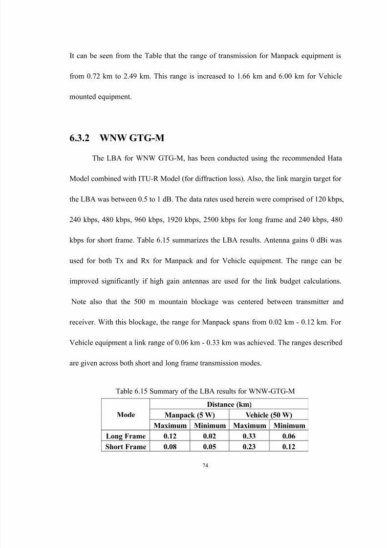
8/8/2019 Oguntade Ayoade Range Estimation for Tactical Radio Waveforms Using Link Budget Analysis
http://slidepdf.com/reader/full/oguntade-ayoade-range-estimation-for-tactical-radio-waveforms-using-link-budget 87/100
74
It can be seen from the Table that the range of transmission for Manpack equipment is
from 0.72 km to 2.49 km. This range is increased to 1.66 km and 6.00 km for Vehicle
mounted equipment.
6.3.2 WNW GTG-M
The LBA for WNW GTG-M, has been conducted using the recommended Hata
Model combined with ITU-R Model (for diffraction loss). Also, the link margin target for
the LBA was between 0.5 to 1 dB. The data rates used herein were comprised of 120 kbps,
240 kbps, 480 kbps, 960 kbps, 1920 kbps, 2500 kbps for long frame and 240 kbps, 480
kbps for short frame. Table 6.15 summarizes the LBA results. Antenna gains 0 dBi was
used for both Tx and Rx for Manpack and for Vehicle equipment. The range can be
improved significantly if high gain antennas are used for the link budget calculations.
Note also that the 500 m mountain blockage was centered between transmitter and
receiver. With this blockage, the range for Manpack spans from 0.02 km - 0.12 km. For
Vehicle equipment a link range of 0.06 km - 0.33 km was achieved. The ranges described
are given across both short and long frame transmission modes.
Table 6.15 Summary of the LBA results for WNW-GTG-M
Mode
Distance (km)
Manpack (5 W) Vehicle (50 W)
Maximum Minimum Maximum Minimum
Long Frame 0.12 0.02 0.33 0.06
Short Frame 0.08 0.05 0.23 0.12

8/8/2019 Oguntade Ayoade Range Estimation for Tactical Radio Waveforms Using Link Budget Analysis
http://slidepdf.com/reader/full/oguntade-ayoade-range-estimation-for-tactical-radio-waveforms-using-link-budget 88/100
75
6.3.3 WNW GTG-U
This is the urban case of the WNW ground to ground propagation cases. The Tx
frequency used for the LBA is 500 MHz. The receiver detection bandwidth of 4 MHz was
also assumed. LBA for WNW GTG-U has been performed using Hata Model for urban
areas. The link margin target for the LBA was between 0.5 to 1. The data rates used
herein were comprised of 120 kbps, 240 kbps, 480 kbps, 960 kbps, 1920 kbps, 2500 kbps
for long frame and 240 kbps, 480 kbps for short frame. Antenna gains of 0 dBi was used
for both Manpack and vehicle mounted equipment. Tx and Rx heights of 1.7 m and Tx
power of 5 W were assumed for Manpack equipment, while Tx and Rx heights of 2.8 m
and Tx power of 50 W were assumed for vehicle mounted equipment. The results of the
LBA are shown in Table 6.16 below.
Table 6.16 Summary of the LBA results for WNW GTG-U
Mode
Distance (km)
Manpack (5 W) Vehicle (50 W)
Maximum Minimum Maximum Minimum
Long Frame 0.62 0.18 1.38 0.38
Short Frame 0.47 0.30 1.05 0.65
The results of Table 6.16 shows that the link range for Manpack spans 0.18 km – 0.62 km
while Vehicle equipment propagation range is between 0.38 km - 1.38 km. The ranges
described are given across both short and long frame transmission modes.

8/8/2019 Oguntade Ayoade Range Estimation for Tactical Radio Waveforms Using Link Budget Analysis
http://slidepdf.com/reader/full/oguntade-ayoade-range-estimation-for-tactical-radio-waveforms-using-link-budget 89/100
76
6.3.4 WNW GTS/STG/STS
Due to the propagation characteristics of the UHF band of the WNW, The ground
length which was present in the mixed mode cases (GTS and STG) of the HFW and
VHFW was removed for the WNW cases. This is because propagated radio waves get
attenuated faster over ground paths at UHF frequencies that VHF or HF frequencies. The
LBA of the WNW cases was performed based on the assumption that the transmitter in
the case of the GTS (or receiver in the case of the STG) is placed at the shore which is the
boundary between land and sea. This means that all the propagation takes place over the
sea and no ground path is included. The LBA results obtained were based on the antenna
gain of 0 dBi for both Tx and Rx, Tx operating frequency of 500 MHz, receiver detection
bandwidth of 4 MHz and Tx power of 5 W and 50 W. The data rates used herein were
comprised of 120 kbps, 240 kbps, 480 kbps, 960 kbps, 1920 kbps, 2500 kbps for long
frame and 240 kbps, 480 kbps for short frame. The link margin target for the LBA was
between 0.5 to 1 dB. The results of the LBA for these three cases are shown in Table 6.17
below.
Table 6.17 Summary of the LBA results for WNW GTS/STG/STS
Optimization
for
Mode
Distance (km)
(5 W) (50 W)
Maximum Minimum Maximum Minimum
Link Margin Long Frame 1.70 0.40 4.50 1.10
Short Frame 1.40 0.70 3.40 2.00

8/8/2019 Oguntade Ayoade Range Estimation for Tactical Radio Waveforms Using Link Budget Analysis
http://slidepdf.com/reader/full/oguntade-ayoade-range-estimation-for-tactical-radio-waveforms-using-link-budget 90/100
77
6.4 Propagation Range with design parameter Variation
Propagation environment, center frequency, transmitter power, antenna height,
antenna gain are major parameters that need to be taken into consideration for the
estimation of propagation range for each of the waveforms. Due to the multivariate nature,
while some parameters are being varied, the remaining parameters had to be held
constant. Since propagation range and data rates are the most important variables of
interest, a series of graphs have been produced as a function of these two parameters,
while varying some parameters. As expected, for the three different waveforms, results
show that the propagation range reduces as data rate is increased. The parameters that
have been varied and plotted in the graphs are: Propagation environment, center
frequency, transmitter power and antenna height.
6.4.1 Range Based on Propagation Environment& Data Rate
The five cases have been shown for each of the waveforms - GTG-O, GTG-M,
GTG-U, STS and GTS (STG) – to show the effect of varying propagation environment
and data rates on propagation range. The graph for the HFW waveform has been plotted
for transmit power of 100 W. This is shown in Figure 6.1. The VHFW waveform graph
was plotted for manpack equipment (Tx power of 5 W) operating in fixed mode which is
represented by the ‘F’ shown in front of the cases in Figure 6.2. Also the WNW graph

8/8/2019 Oguntade Ayoade Range Estimation for Tactical Radio Waveforms Using Link Budget Analysis
http://slidepdf.com/reader/full/oguntade-ayoade-range-estimation-for-tactical-radio-waveforms-using-link-budget 91/100
78
was plotted for manpack equipment which operates in the long frame mode. This is
depicted by ‘L’ that is shown in Figure 6.3. At any data rate, for all the HFW and VHFW
waveforms, the STS case produced the longest range. This is due to the excellent sea
conductivity as compared to ground. This was followed by GTS case. The deviation from
this ideal is observed in the WNW case due to the high frequency on which it operates
which consequentially makes the MGPP propagation model to break down.
Figure 6.1 Range vs Data rate for HFW cases
Figure 6.2 Range vs Data rate for VHFW Cases

8/8/2019 Oguntade Ayoade Range Estimation for Tactical Radio Waveforms Using Link Budget Analysis
http://slidepdf.com/reader/full/oguntade-ayoade-range-estimation-for-tactical-radio-waveforms-using-link-budget 92/100
79
Figure 6.3 Range vs Data rate for WNW Cases
6.4.2 Range Based on Center Frequency
To see the effect of change of transmitter center frequency on the WNW propagation
range as in, the graph of range vs. data rate at four different centre frequencies were
plotted. These are shown in Figure 6.4. The frequencies are – 250, 350, 500 and 1,300
MHz. The WNW GTG-U case with transmitter power fixed at 50 W is used here as a case
study. Also, the average range increase at the 6 data rates has been used. It can be
observed form the graph that when the centre frequency is reduced from 1300 MHz to
500 MHz, the propagation range improves by a factor of about 1.8 (the average of the
range increase at the 6 different data rates). A range increase by a factor of about 1.25 is
further noticed when the 500 MHz center frequency is reduced to 350 MHz. As the
frequency is reduced to 250 MHz, the corresponding range is increased by a factor of
about 1.23. This corresponds to an overall range increase by a factor of about 2.3 when

8/8/2019 Oguntade Ayoade Range Estimation for Tactical Radio Waveforms Using Link Budget Analysis
http://slidepdf.com/reader/full/oguntade-ayoade-range-estimation-for-tactical-radio-waveforms-using-link-budget 93/100
80
center frequency is reduced from 1300 to 250 MHz. Considering the 500 MHz center
frequency used for this work, the range can be improved by a factor of about 1.5 if the
center frequency is changed to 250 MHz.
Figure 6.4 Range vs Data rate for WNW GTG-U
at different frequncies.
6.4.3 Range Based on Transmitter Power
As in the case of center frequency parameter, the WNW GTG-U case has been used to the
see the effect of varying transmitter power on propagation range. Here, shown in Figure
6.5, center frequency and antenna height are fixed to 500 MHz and 2.8 m respectively.
When the power is increased from 5 W to 50 W, the range is increased by a factor of
about 1.96.

8/8/2019 Oguntade Ayoade Range Estimation for Tactical Radio Waveforms Using Link Budget Analysis
http://slidepdf.com/reader/full/oguntade-ayoade-range-estimation-for-tactical-radio-waveforms-using-link-budget 94/100
81
Figure 6.5 Range vs Data rate for WNW GTG-U
for different Tx powers.
As the power is doubled from 50 W to 100 W, the propagation range correspondingly
increases by a factor of about 1.18. A factor of 1.1 range increase is observed when Tx
power is increased from 100 W to 150 W. The overall range increase from 5 W to 150 W
is a factor 2.24. This shows that the transmitter power variation produces the same overall
result in range increase as in the variation of center frequency.
6.4.4 Range Based on Antenna Height
Figure 6.6 shows the effect of varying antenna height on the range of propagation for the
WNW GTG-U. Four different antenna heights have been used. These are – 1.7 m, 2.7 m,
2.8 m and 4 m. Tx power of 5 W was used for the 1.7 and 2.7 m curves – being manpack
equipment, while the 2.8 and 4 m curves – being vehicle mounted equipment – were

8/8/2019 Oguntade Ayoade Range Estimation for Tactical Radio Waveforms Using Link Budget Analysis
http://slidepdf.com/reader/full/oguntade-ayoade-range-estimation-for-tactical-radio-waveforms-using-link-budget 95/100
82
plotted using Tx power of 50 W. It can be observed from the graph that as the antenna
height is increased from 1.7 m to 2.7 m, the propagation range improves by a factor of
about 1.1. The same range increase factor - about 1.1 - is also observed when the antenna
height of 2.8 is increased to 4 m.
Figure 6.6. Range vs Data rate for WNW GTG-U
for different antenna heights.

8/8/2019 Oguntade Ayoade Range Estimation for Tactical Radio Waveforms Using Link Budget Analysis
http://slidepdf.com/reader/full/oguntade-ayoade-range-estimation-for-tactical-radio-waveforms-using-link-budget 96/100
83
Chapter 7
Conclusion and Future Work
The performance of three disparate waveforms (HFW, VHFW and the WNW) which
are of interest to tactical communications have been discussed under different
propagation environment. Several propagation models were used in the estimation of
Path loss that are typical of these environment and the propagation range for these
waveforms under these conditions have been suggested. The propagation range for these
waveforms were estimated for two equipment types: Manpack and Vehicle mounted
equipment. The extent to which the range changed when equipment design parameters
were varied was also discussed. The five design parameters considered were: Transmitter
power, center frequency, antenna gain, antenna height and data rate. Each of the three
waveforms has its own advantages and drawbacks. While the HFW is the choice
waveform for BLOS communications - notwithstanding its inherent problem of low data
rates, the demand for high data rate and networking capabilities makes the WNW
extremely attractive for use in where these goals need to be met.

8/8/2019 Oguntade Ayoade Range Estimation for Tactical Radio Waveforms Using Link Budget Analysis
http://slidepdf.com/reader/full/oguntade-ayoade-range-estimation-for-tactical-radio-waveforms-using-link-budget 97/100
84
7.1 Conclusion
The conclusions arrived at from the results are summarized as below:
1) The design parameter that yielded the greatest improvement in propagation range was
identified. The reduction in the center operating frequency gave the best result in a
increasing propagation range. The increase in antenna height produced the least result
in range improvement.
2) In performing the LBA, it was noticed that the ambient temperature of the receiver
can adversely affect its sensitivity which consequentially affects range due to the
increase in thermal noise power across the detection bandwidth.
3) The HFW produced the longest range of all the three waveforms. This was followed
by the VHFW. The propagation range of the WNW was shortest; albeit it provided the
highest data rate.
4) Since there are practical limits to which most of the design factors like transmitter
power, antenna gain, antenna heights can be exploited, use of channel coding surely
can improve the performance of the waveforms and enhanced propagation range.
7.2 Future Work
The following areas offer further research based on the outcome of this thesis.
1) Other code rates for the convolution codes used could be investigated for all the

8/8/2019 Oguntade Ayoade Range Estimation for Tactical Radio Waveforms Using Link Budget Analysis
http://slidepdf.com/reader/full/oguntade-ayoade-range-estimation-for-tactical-radio-waveforms-using-link-budget 98/100
85
waveforms to see whether the bit error rate and range improve.
2) More waveforms of interest to tactical communications could be investigated.
3) Low Density Parity Check codes could be used for the WNW instead of
convolution codes. Recent findings have shown that LDPC performs better with
OFDM waveform due to its low error floor and performance at high code rates.
4) Since most modern radio equipment technology (like the IEEE 802.11n) gravitate
towards MIMO that takes advantage of space diversity to improve range and data
rate, work should be done on using multiple antennas for these equipment. The
fading channel also need to be modeled as a Nakagami-m channel since it
characterizes fading in the MIMO context.

8/8/2019 Oguntade Ayoade Range Estimation for Tactical Radio Waveforms Using Link Budget Analysis
http://slidepdf.com/reader/full/oguntade-ayoade-range-estimation-for-tactical-radio-waveforms-using-link-budget 99/100
86
References
[1] JTRS Joint Program Office, JTRS Wideband Networking Waveform (WNW)
Functional Description Document (FDD) Version 2.21, November 2001.
[2] North, R., “Joint Tactical Radio System – Connecting the GIG to the Tactical Edge”,
proceedings of MILCOM 2006, Washington DC, October 2006.
[3] Chryssomallis, M., and Chrlstodoulou, C., “Simulation of Mobile Fading Channels”,
IEEE Antennas and Propagation Magazine , Vol. 44, No. 6, December 2002, pp. 172– 183.
[4] Van Nee, R. and Prasad, R., “OFDM for Wireless Multimedia Communications”,
Artech House Publishers, 2000.
[5] Kabulepa, L.D., “OFDM Basics for wireless communications”, Institute of
Microelectronics system, Darmstadt University of Tech, 2004.
[6] Kim, J., Oguntade, A., Oza M., and Kim, S., “Range Estimation for Tactical Radio
Waveforms Using Link Budget Analysis”, proceedings of IEEE Milcom Conference,
Boston, MA, October 2009.
[7] Hata, M., “Empirical Formulae for Propagation Loss in Land Mobile Radio Services,”
IEEE Trans.Vehic. Tech., vol. VT-29, no. 3, 1980, pp. 317–325.
[8] Egli, John J. "Radio Propagation Above 40 MC Over Irregular Terrain." Proceedings
of the IRE 45, no. 10 (1957): pp 1383-1391.
[9] International Telecommunication Union website: www.itu.int.
[10] Barclay, L., Propagation of Radiowaves, 2nd
ed., London: The Institution of Electrical Engineers, 2003.
[11] Millington, G., "Groundwave Propagation over an Inhomogeneous Smooth Earth",IEE Proceedings, 96 Part III, p.53, Mar 1949.
[12] Sevgi, L., "A Mixed-Path Groundwave Field Strength Prediction Virtual Tool for Digital Radio Broadcast Systems in Medium and Short Wave Bands", IEEE
Antennas and Propagation Magazine, Vol. 48, No.5, Oct 2006.

8/8/2019 Oguntade Ayoade Range Estimation for Tactical Radio Waveforms Using Link Budget Analysis
http://slidepdf.com/reader/full/oguntade-ayoade-range-estimation-for-tactical-radio-waveforms-using-link-budget 100/100
[13] Sevgi, L., Complex Electromagnetic Problems and Numerical Simulation
Approaches, Wiley-IEEE, 2003.
[14] Luo Lichun, “A new MF and HF Ground-wave Model for Urban Areas”, IEEE
Antennas and Propagation Magazine, Vol. 42, No 1, February 2000, pp. 21-33.
[15] Hall, M.P.M., Effects of the troposphere on Radio Communication, Peter
Pergrinus, 1979.
[16] Fabio Belloni, “Fading models” S-88 Signal Processing Laboratory, HUT.
[17] Karagiannidis G, N-Nakagami “A Novel Stochastic Model for Cascaded Fading
Channels”, IEEE Transactions on Communications, vol. 55, No 8, August 2007, pp.
1453–1458.
[18] Crepeau, P.J.: ‘Uncoded and coded performance of MFSK and DPSK in Nakagami
fading channels’, IEEE Transactions on Communications, March 1992, Vol 40, pp.
487–493.
[19] MIL-STD-188-110B specifications.
[20] Junghwan Kim, Mike Orra, Chong Wang, Ayoade Oguntade, Oza Maulik, and
Pooja Raorane, “Final Report of Link Budget Analysis for the Radio System”,
Submitted to LIGNEX1 Co., Ltd, 2008.
[21] Rao, T. R., and Vijaya, S., “Single Knife edge diffraction propagation studies
over a hilly terrain”, IEEE Transactions on Broadcasting, vol. 45, no.1, March
1999, pp. 20-29.