Embed Size (px)
Citation preview
OFFICIAL MASTER´S DEGREE IN THE ELECTRIC POWER
INDUSTRY
Master´s thesis
ECONOMIC ANALYSIS OF THE INCREASE IN NUMBER
OF INTRADAY MARKET SESSIONS IN THE IBERIAN
MARKET
Author: Manuel Allo Pérez
Director: Juan Bogas Gálvez
Madrid, July 2016


OFFICIAL MASTER´S DEGREE IN THE ELECTRIC POWER
INDUSTRY
Master´s thesis
ECONOMIC ANALYSIS OF THE INCREASE IN NUMBER
OF INTRADAY MARKET SESSIONS IN THE IBERIAN
MARKET
Author: Manuel Allo Pérez
Director: Juan Bogas Gálvez
Madrid, July 2016

4
Contents index
Abstract .................................................................................................................................... 9
Resumen ................................................................................................................................. 10
1. Introduction ................................................................................................................... 11
2. Objectives of the Master Thesis ................................................................................... 13
3. Description of the Iberian Market ................................................................................ 14
3.1. Forward Contracts: ...................................................................................................... 14
3.2. Day Ahead Market: ..................................................................................................... 15
3.3. Intraday Markets: ........................................................................................................ 17
3.4. Balancing Markets: ...................................................................................................... 19
3.4.1 Deviations management ......................................................................................... 20
3.4.2 Tertiary regulation ................................................................................................... 21
3.4.3 Secondary regulation .............................................................................................. 23
3.5. Other markets ............................................................................................................. 25
3.6. Final Program (P48) ..................................................................................................... 26
4. Deviations ....................................................................................................................... 27
4.1. Deviation causers ........................................................................................................ 29
4.1.1 Main drivers on consumer’s deviations .................................................................. 30
4.1.2 Main drivers on wind deviations ............................................................................. 31
4.1.3 Main drivers on solar deviations ............................................................................. 32
5. Classification of ID operations ...................................................................................... 33
5.1 Agents behavior .......................................................................................................... 33
5.1.1 No time to renegotiate ............................................................................................ 33
5.1.2 Reschedule down on ID ........................................................................................... 34
5.1.3 Reschedule up on next ID ........................................................................................ 35
5.1.4 Speculative behavior / error ................................................................................... 35
5.1.5 Expect to fix the problem before incurring on a deviation ..................................... 38

5
5.1.6 There is no deviation ............................................................................................... 38
5.2 Classification by number of operations ...................................................................... 39
5.3 Classification by volume of energy traded .................................................................. 39
5.3.1 Volumes negotiated to increase production .......................................................... 40
5.3.2 Volumes negotiated to decrease production ........................................................ 41
6. Economic impact of current Intraday Market ............................................................. 43
6.1 Impact for thermal units: ............................................................................................ 44
7. Design of the new Intraday Market ............................................................................. 45
7.1 Expected prices of the new market design ................................................................. 48
7.2 Expected volumes of the new design .......................................................................... 50
8. Economic analysis of new Intraday Market ................................................................. 52
8.1 Deviations price ........................................................................................................... 52
8.2 Deviations volume for thermal units .......................................................................... 55
8.3 Variation on Intraday operations for thermal units .................................................... 56
8.4 Impact on thermal units .............................................................................................. 57
9. Conclusions .................................................................................................................... 61
10. Bibliography ................................................................................................................... 64
6
Figures index
Chart 1. Spanish energy markets scheduling .............................................................................. 14
Chart 2. Market clearing. Source: OMIE ...................................................................................... 16
Chart 3. Monthly DAM prices. Source: OMIE .............................................................................. 17
Chart 4. Day ahead and Intraday scheduling. Source: OMIE ...................................................... 18
Chart 5. Intraday market scheduling. Source: OMIE ................................................................... 18
Chart 6. Average prices per session ............................................................................................ 19
Chart 7. Deviations management pricing. Source: REE ............................................................... 21
Chart 8. Energy managed on deviations management. Source: REE .......................................... 21
Chart 9. Pricing of deviation management procedure. Source: REE ........................................... 21
Chart 10. Tertiary reserve pricing. Source: REE .......................................................................... 22
Chart 11. Energy managed on tertiary reserve. Source: REE ...................................................... 22
Chart 12. Pricing of tertiary reserve. Source: REE ....................................................................... 23
Chart 13. Secondary regulation pricing. Source: OMIE ............................................................... 24
Chart 14. Energy managed on secondary reserve. Source: REE ................................................. 24
Chart 15. Pricing of secondary reserve. Source: REE .................................................................. 25
Chart 16. Average band of secondary reserve. Source: REE ....................................................... 25
Chart 17. Secondary reserve band pricing. Source: REE ............................................................. 25
Chart 18. Final price components. Source: REE .......................................................................... 26
Chart 19. Deviations pricing ........................................................................................................ 27
Chart 20. Example of deviations pricing ...................................................................................... 28
Chart 21. Deviations economic loss ............................................................................................ 28
Chart 22. Deviation volumes by technology ............................................................................... 29
Chart 23. Correlation between deviation and technology .......................................................... 30
Chart 24. Typical daily load profile. Source. REE ......................................................................... 31
7
Chart 25. Intraday market scheduling. Source: OMIE ................................................................. 34
Chart 26. No time to renegotiate example ................................................................................. 34
Chart 27. Reschedule down on ID example ................................................................................ 35
Chart 28. Reschedule up on ID example ..................................................................................... 35
Chart 29. Speculative behavior example 1 .................................................................................. 36
Chart 30. Speculative behavior example 2 .................................................................................. 36
Chart 31. Speculative behavior example 3 .................................................................................. 37
Chart 32. Speculative behavior example 4 .................................................................................. 37
Chart 33. Speculative behavior example 5 .................................................................................. 37
Chart 34. Speculative behavior example 6 .................................................................................. 38
Chart 35. Expectation to fix the problem example ..................................................................... 38
Chart 36. No deviation example .................................................................................................. 38
Chart 37. Breakdown of ID operations ........................................................................................ 39
Chart 38. Volume of ID operations to increase energy ............................................................... 40
Chart 39. Energy to increase production .................................................................................... 41
Chart 40. Volume of ID operations to reduce energy ................................................................. 41
Chart 41. Energy to decrease production ................................................................................... 42
Chart 42. Intraday sessions scheduling ....................................................................................... 43
Chart 43. Benefits of current ID on thermal units ....................................................................... 44
Chart 44. Waiting time under current ID model ......................................................................... 45
Chart 45. New ID scheduling ....................................................................................................... 46
Chart 46. Waiting times for new ID ............................................................................................. 46
Chart 47. Hourly distribution of thermal outages ....................................................................... 47
Chart 48. Comparison between current and future ID waiting times ........................................ 48
Chart 49. Average ID prices per session ...................................................................................... 49
Chart 50. Average ID market prices ............................................................................................ 49
8
Chart 51.Intraday volumes per session. Source: OMIE ............................................................... 50
Chart 52. System needs pricing ................................................................................................... 52
Chart 53. Regression analysis ...................................................................................................... 53
Chart 54. Correlation deviation volume – system loss (system up) ............................................ 54
Chart 55. Correlation deviation volume - system loss (system down) ....................................... 54
Chart 56. Deviation cost estimation ............................................................................................ 55
Chart 57. Deviation volume under current and new model ....................................................... 55
Chart 58. Expected energy to increase production ..................................................................... 56
Chart 59. Expected energy to decrease production ................................................................... 56
Chart 60. Number of current operations vs expected ................................................................ 57
Chart 61. Income variation under different schemes ................................................................. 57
Chart 62. Hours with deviations, separated by system requirements........................................ 58
Chart 63. Cost estimation for new ID .......................................................................................... 58
Chart 64. Income estimation for new ID ..................................................................................... 59
Chart 65. Expected benefits of new ID, compared with current ID ............................................ 59
Chart 66. Expected benefits of new ID, compared with DAM .................................................... 60
Chart 67. Spanish and French spot prices, 2015. Source: OMEL ................................................ 61
Chart 68. Status of the interconnection capacity ....................................................................... 62


9
Abstract
This project aims to assess the economic impact on thermal plants with outages due to a
forecasted increase of the number of sessions of the intraday market, from the current six to
twenty-four, one every hour.
In order to estimate the economic impact, it has been needed to quantify the current cost of
the adjustment services, such as the tertiary regulation, secondary regulation and deviation
management, used to correct the current deviations. In addition, it is necessary to infer the
behavior of agents, i.e, why they operate as they do under the current model.
An estimation of volumes traded under the new model was obtained, as well as prices, both
from intraday operations and adjustment services.
A reasonable estimation of the savings for thermal units with the new model was obtained.

10
Resumen
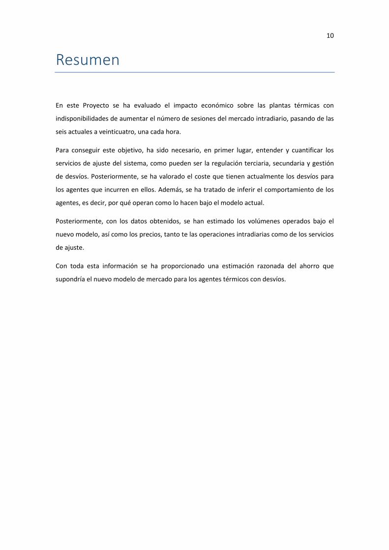
En este Proyecto se ha evaluado el impacto económico sobre las plantas térmicas con
indisponibilidades de aumentar el número de sesiones del mercado intradiario, pasando de las
seis actuales a veinticuatro, una cada hora.
Para conseguir este objetivo, ha sido necesario, en primer lugar, entender y cuantificar los
servicios de ajuste del sistema, como pueden ser la regulación terciaria, secundaria y gestión
de desvíos. Posteriormente, se ha valorado el coste que tienen actualmente los desvíos para
los agentes que incurren en ellos. Además, se ha tratado de inferir el comportamiento de los
agentes, es decir, por qué operan como lo hacen bajo el modelo actual.
Posteriormente, con los datos obtenidos, se han estimado los volúmenes operados bajo el
nuevo modelo, así como los precios, tanto te las operaciones intradiarias como de los servicios
de ajuste.
Con toda esta información se ha proporcionado una estimación razonada del ahorro que
supondría el nuevo modelo de mercado para los agentes térmicos con desvíos.


11
1. Introduction
The Iberian Electricity market, as many others in the world, allows buyers and sellers to trade
under different contracting options: the Forward Markets, as the ones managed by OMIP, Day
Ahead and Intraday markets, managed by OMIE (Iberian Market Operator), and Ancillary
services market, managed by Red Electrica de España (REE, the Spanish System Operator). The
most important one is the Day-ahead market, because it is the one in which the vast majority
of the energy is assigned. This market is not mandatory, since bilateral contracts are allowed.
The European Commission has established a Target Model for Intraday, based on continuous
energy trading where cross-zonal transmission capacity is allocated through implicit
continuous allocation, with the possibility to run regional intraday auctions. This model has
been laid down into the Framework Guidelines for Capacity Allocation and Congestion
Management (CACM).
The European Power Exchanges APX, Belpex, EPEX Spot, GME, Nord Pool and OMIE are
responding to the needs of the market by establishing a transparent and efficient continuous
intraday trading environment to enable market parties to easily trade out their intraday
positions. The possibility for market parties to trade out their imbalances will thereby be
significantly improved as they do not only benefit from the national available intraday liquidity,
but also from the available liquidity in other areas. Later on in the Iberian market there will be
national intraday sessions in order to be able to offer the net position in the continuous
trading.
In order to help to realize this goal of a continuous trading, the PXs, together with the
Transmission System Operators from 12 countries, have launched an initiative called the XBID
Market Project to create a joint integrated intraday cross-zonal market. The purpose of the
XBID Market Project is to enable continuous cross-zonal trading and increase the overall
efficiency of intraday trading on the single cross-zonal intraday market across Europe. The
wider XBID solution will create one integrated European Intraday market.
This single Intraday cross-zonal market solution will be based on a common IT system forming
the backbone of the European solution, linking the local trading systems operated by the
Power Exchanges, as well as the available cross-zonal transmission capacity provided by the
TSOs. Agents will participate in a portfolio base. Orders entered by market participants in one
country can be matched by orders similarly submitted by market participants in their own

12
country or in any other country interconnected, provided there is cross-zonal capacity
available. XBID market solution allows, apart from the continuous trading, to implement
periodic regional auctions. The Iberian scheme will be based on 24 intraday sessions, in order
to schedule a physical program for every unit instead of 6 sessions as today.
Additionally, due to the volatility of renewables, the necessity to trade these units as close to
real time as possible has become necessary. In order to do so, it is possible to increase the
number of intraday sessions even before the implementation of the continuous trading.

13
2. Objectives of the Master Thesis
The objectives of this master thesis are shown below:
To understand the ancillary services markets and its economic impact: understand
how tertiary, secondary and deviations management, are used to keep the system
balanced and how are they priced.
To assess the economic cost of thermal plants deviations, due to unexpected outages,
under current model: Once the deviation cost is calculated, it is needed to analyze the
agent’s behavior and their ability to renegotiate on Intraday Sessions and, in case of
failure, the expected deviation costs.
To estimate the impact of covering those deviations on a new scheduled intraday
market: With an increased number of intraday sessions, the agents will have more
opportunities to renegotiate their production and reduce their deviation costs.
To show the savings achieved: by comparing the current model with the proposed one.
To estimate the volume/price of transactions on this market.

14
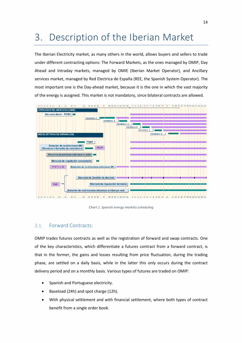
3. Description of the Iberian Market
The Iberian Electricity market, as many others in the world, allows buyers and sellers to trade
under different contracting options: The Forward Markets, as the ones managed by OMIP, Day
Ahead and Intraday markets, managed by OMIE (Iberian Market Operator), and Ancillary
services market, managed by Red Electrica de España (REE, the Spanish System Operator). The
most important one is the Day-ahead market, because it is the one in which the vast majority
of the energy is assigned. This market is not mandatory, since bilateral contracts are allowed.
Chart 1. Spanish energy markets scheduling
3.1. Forward Contracts:
OMIP trades futures contracts as well as the registration of forward and swap contracts. One
of the key characteristics, which differentiate a futures contract from a forward contract, is
that in the former, the gains and losses resulting from price fluctuation, during the trading
phase, are settled on a daily basis, while in the latter this only occurs during the contract
delivery period and on a monthly basis. Various types of futures are traded on OMIP:
Spanish and Portuguese electricity.
Baseload (24h) and spot charge (12h).
With physical settlement and with financial settlement, where both types of contract
benefit from a single order book.
15
With maturities of days, weekends, weeks, months, quarters and years.
Besides providing a registration platform for OTC transactions to be cleared on OMIClear, for
all these futures contracts, OMIP also allows the registration of forward and swap trades:
Foreseeing for the former, physical delivery and settlement of VAT and for the latter, a
purely financial settlement excluding VAT.
Both on Spanish and Portuguese electricity.
With the same maturities as futures contracts.
The size of all of these contracts is 1 MW, with a 0.01 Euros/MWh tick.
3.2. Day Ahead Market:
The daily market is the main market for contracting electricity in the Iberian Peninsula. It
operates 365 days a year and is managed by the Market Operator, OMIE. On it, buying and
selling transactions are carried out for the next day. It is a marginal market where price and
volume for each hour of programming the next day is set at the matching point between
supply and demand. This market is operated by OMIE for the Spanish and Portuguese system.
Agents must submit their offers before 12 am of the previous day to the delivery day. Each
offer consists of energy terms in MWh with their corresponding hourly prices in €/MWh. Sale
bids may be simple or incorporate complex conditions in terms of their content. Sellers for
each hour and production unit can present simple bids, indicating a price and an amount of
power. Complex bids are those that incorporate complex sale terms and conditions and those
which, in compliance with the simple bid requirements, also include one or some of the
following technical or economic conditions:
Indivisibility: The indivisibility condition enables a minimum operating value to be
fixed in the first block of each hour. This value may only be divided by applying
distribution rules if the price is other than zero.
Load gradients: The load gradient enables the maximum difference between the
energy in one hour and the energy in the following hour of the production unit to be
established, limiting maximum matchable energy by matching the previous hour and
the following hour, in order to avoid sudden changes in the production units that the
latter are unable to follow from a technical standpoint.
16
Minimum income: The minimum income condition enables bids to be presented in all
hours, provided that the production unit does not participate in the daily matching
result if the total production obtained by it in the day does not exceed an income level
above an established amount, expressed in euros, plus a variable remuneration
established in euros for every matched MWh.
Scheduled stop: The condition of scheduled stop enables production units that have
been withdrawn from the matching process because they fail to comply the stipulated
minimum income condition to carry out a scheduled stop for a maximum period of
three hours, avoiding stoppages in their schedules from the final hour of the previous
day to zero in the first hour of the following day, by accepting the first slot of first
three hours of their bids as simple bids, the only condition being that energy offered in
bids must drop in each hour.
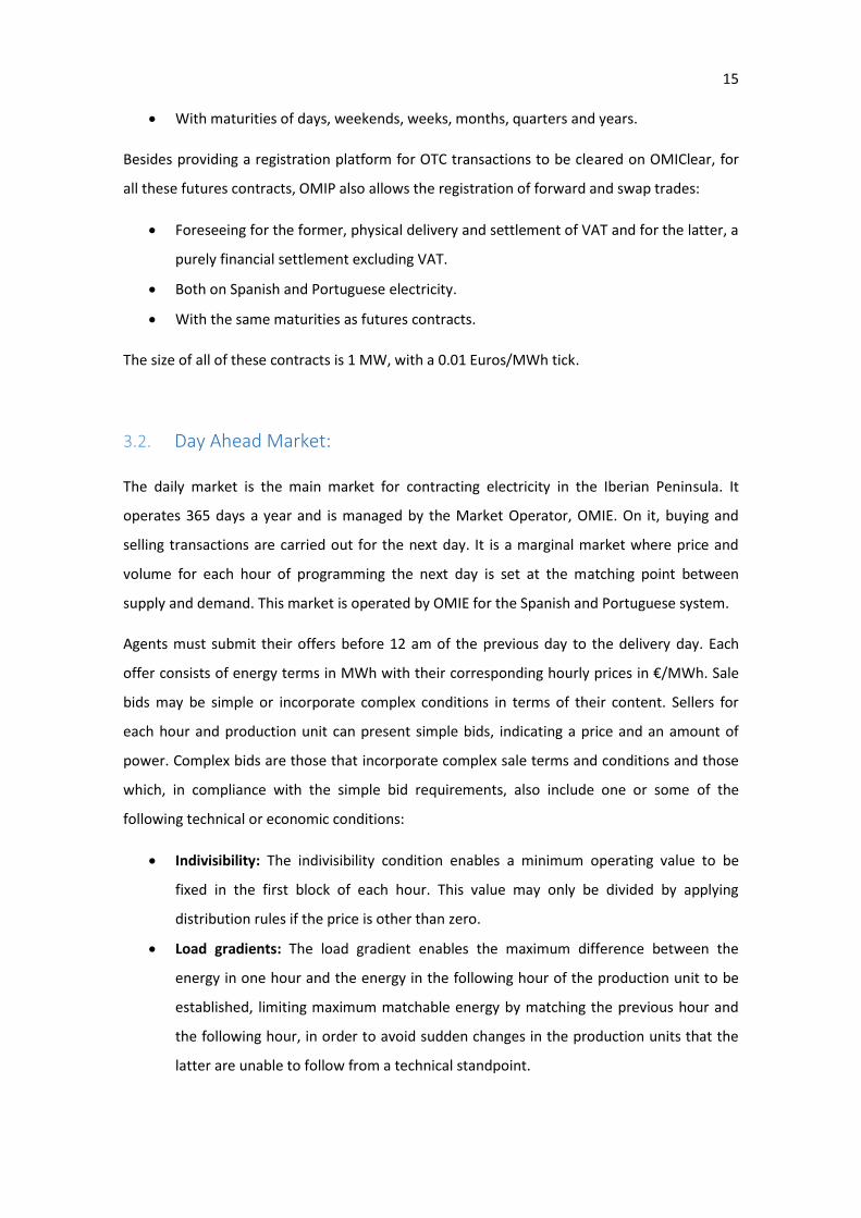
The above mentioned offers are shown jointly with bilateral contracts with physical delivery in
ascending order of bid prices thus forming the aggregate supply curve (bilateral contracts are
evaluated at 0€/MWh for sales and at 180.3 €/MWh for purchases, but only for volume issues,
since they are not really offering any energy in the Day Ahead Market).
Similarly, purchase offers curve is developed. In this case, offers are sorted by descending
price. After the bid acceptance, a matching process, run by EUPHEMIA algorithm, sets the daily
market price, which is marginal and equal to every agent on the Iberian market, unless there is
a congestion in the transmission lines connecting Spain and Portugal. When that happens,
both markets are cleared separately (market splitting).
Chart 2. Market clearing. Source: OMIE
17
This matching process is the Daily Base Operating Program (PDBF), daily energy program
programming periods breakdown of the different programming units corresponding to sales
and purchases of electricity.
Day Ahead market price
Day ahead market price varies for several reasons, as:
RES penetration: windy days are cheaper, as windfarms bid on the market as close to
zero price. A wet month, with plenty of water, brings cheaper energy to the system
and vice versa.
Day of the week: Weekdays usually are more expensive than weekends.
Hour of the day: Peak hours are more expensive than off peak hours.
System needs: If the system need energy, prices will rise and vice versa.
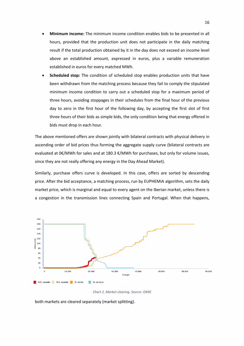
Month of the year: As can be appreciated on chart 3, there is a big difference on
monthly DAM prices. This is due to the reasons mentioned above, but also to the
average temperature. Colder and Hotter months, above and below the comfort
temperature for humans, the need of air conditioning and heating systems which
increase electricity demand and its pricing.
The average Day Ahead price for 2015 was 50.3€/MWh. Detailed monthly prices are shown
below:
Day Ahead prices (€/MWh)
Jan Feb Mar Apr May Jun
53,54 44,62 44,24 46,59 45,91 55,52
Jul Aug Sept Oct Nov Dec
60,53 56,71 52,62 50,84 52,68 54,39 Chart 3. Monthly DAM prices. Source: OMIE
3.3. Intraday Markets:
The intraday market allows different market players to make their adjustments with respect to
the Definitive Viable Daily Schedule (resulting from daily market, bilateral contract and the
resolution of technical restrictions) by submitting bids for sale and purchase of electricity. The
need to make adjustments to the program may be due to changes in the wind/sun forecast for
renewable energy, unforeseen production outages for conventional units or demand forecast
changes.
18
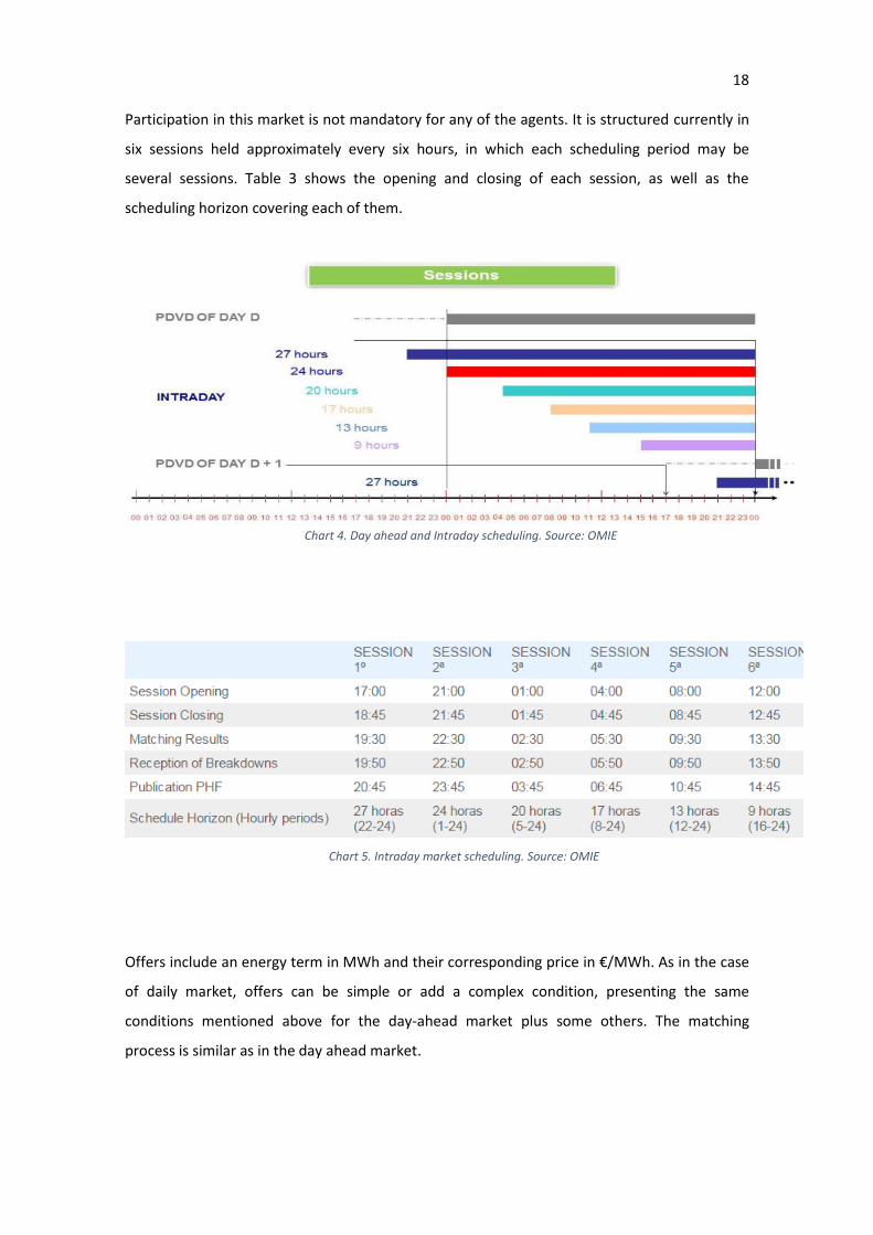
Participation in this market is not mandatory for any of the agents. It is structured currently in
six sessions held approximately every six hours, in which each scheduling period may be
several sessions. Table 3 shows the opening and closing of each session, as well as the
scheduling horizon covering each of them.
Offers include an energy term in MWh and their corresponding price in €/MWh. As in the case
of daily market, offers can be simple or add a complex condition, presenting the same
conditions mentioned above for the day-ahead market plus some others. The matching
process is similar as in the day ahead market.
Chart 4. Day ahead and Intraday scheduling. Source: OMIE
Chart 5. Intraday market scheduling. Source: OMIE
19
The sum of the day ahead and intraday offers shall not exceed the technical limitations of the
power units.
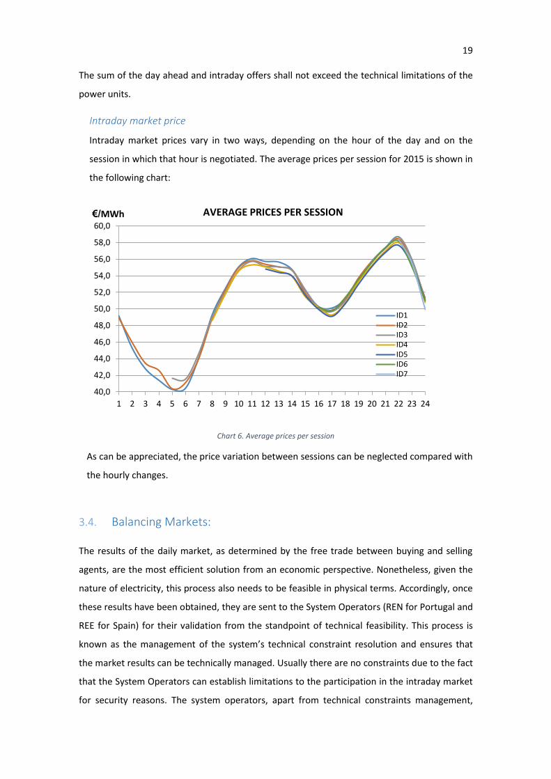
Intraday market price
Intraday market prices vary in two ways, depending on the hour of the day and on the
session in which that hour is negotiated. The average prices per session for 2015 is shown in
the following chart:
Chart 6. Average prices per session
As can be appreciated, the price variation between sessions can be neglected compared with
the hourly changes.
3.4. Balancing Markets:
The results of the daily market, as determined by the free trade between buying and selling
agents, are the most efficient solution from an economic perspective. Nonetheless, given the
nature of electricity, this process also needs to be feasible in physical terms. Accordingly, once
these results have been obtained, they are sent to the System Operators (REN for Portugal and
REE for Spain) for their validation from the standpoint of technical feasibility. This process is
known as the management of the system’s technical constraint resolution and ensures that
the market results can be technically managed. Usually there are no constraints due to the fact
that the System Operators can establish limitations to the participation in the intraday market
for security reasons. The system operators, apart from technical constraints management,
40,0
42,0
44,0
46,0
48,0
50,0
52,0
54,0
56,0
58,0
60,0
1 2 3 4 5 6 7 8 9 10 11 12 13 14 15 16 17 18 19 20 21 22 23 24
ID1ID2ID3ID4ID5ID6ID7
AVERAGE PRICES PER SESSION€/MWh
20
establish tertiary regulation, secondary regulation and deviations management markets. The
prices of these markets are usually higher than the Day ahead and Intraday ones, due to the
cost of keeping some plants on standby and ready to produce with only some minutes of
notification, or even to curtail their production to allow them some margin in order to solve
contingencies.
3.4.1 Deviations management
The purpose of this procedure is to solve the deviations between generation and
consumption that may appear between the close of each intraday market session and the
start of the horizon effectiveness of the next session. Deviation management plays a role as
a link between the intraday markets and real time management, providing the System
Operator with a competitive market service, and greater flexibility to solve imbalances
between generation and demand, identified after the intraday market, without
compromising the availability of required reserves for secondary and tertiary regulation.
Before each hour, planed/unplanned deviations within the time horizon until the next
session of the intraday market are assessed and, if the volume identified is higher than 300
MWh, held several hours, the system operator can proceed to convene the market
deviation management.
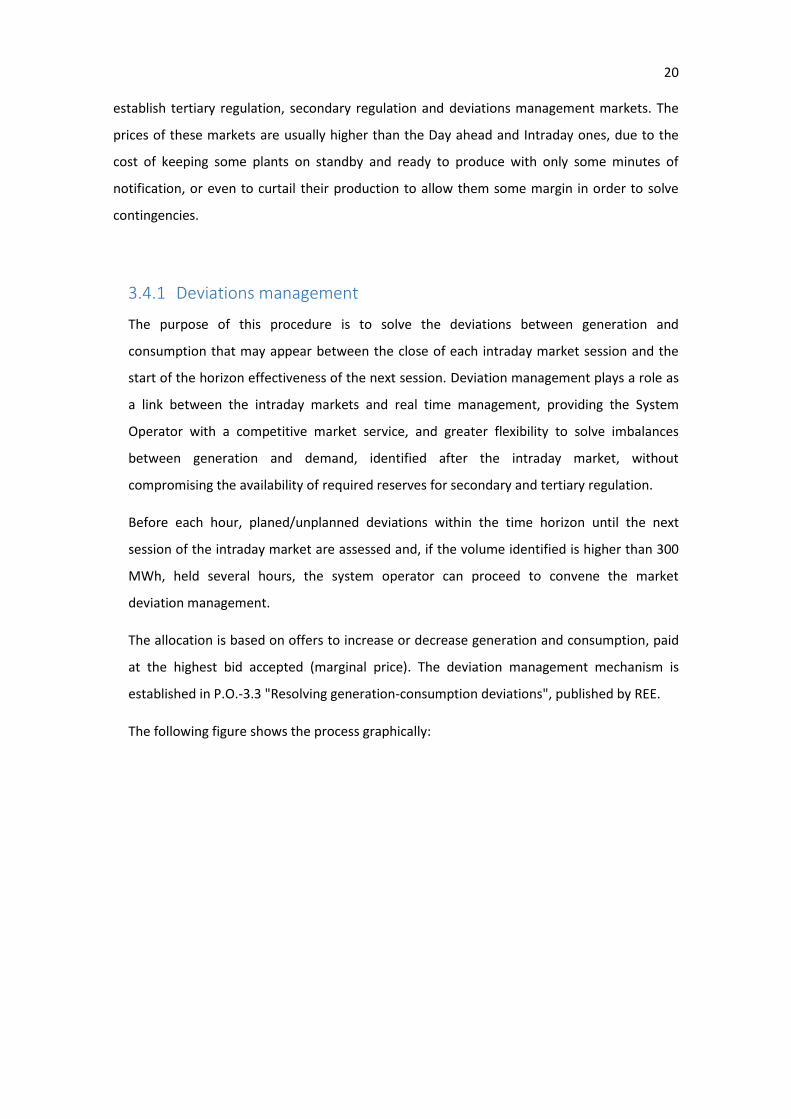
The allocation is based on offers to increase or decrease generation and consumption, paid
at the highest bid accepted (marginal price). The deviation management mechanism is
established in P.O.-3.3 "Resolving generation-consumption deviations", published by REE.
The following figure shows the process graphically:
21
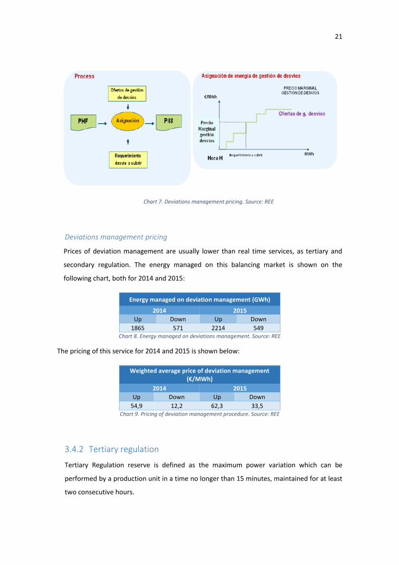
Deviations management pricing
Prices of deviation management are usually lower than real time services, as tertiary and
secondary regulation. The energy managed on this balancing market is shown on the
following chart, both for 2014 and 2015:
Energy managed on deviation management (GWh)
2014 2015
Up Down Up Down
1865 571 2214 549 Chart 8. Energy managed on deviations management. Source: REE
The pricing of this service for 2014 and 2015 is shown below:
Weighted average price of deviation management (€/MWh)
2014 2015
Up Down Up Down
54,9 12,2 62,3 33,5 Chart 9. Pricing of deviation management procedure. Source: REE
3.4.2 Tertiary regulation
Tertiary Regulation reserve is defined as the maximum power variation which can be
performed by a production unit in a time no longer than 15 minutes, maintained for at least
two consecutive hours.
Chart 7. Deviations management pricing. Source: REE
22
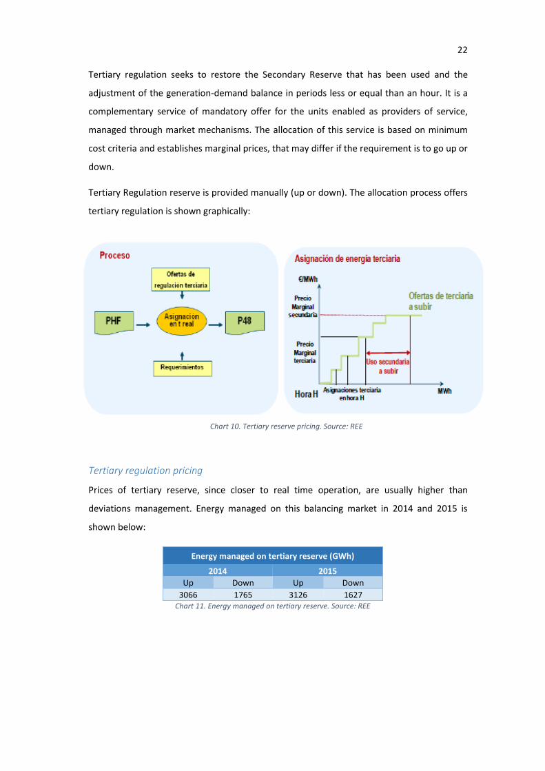
Tertiary regulation seeks to restore the Secondary Reserve that has been used and the
adjustment of the generation-demand balance in periods less or equal than an hour. It is a
complementary service of mandatory offer for the units enabled as providers of service,
managed through market mechanisms. The allocation of this service is based on minimum
cost criteria and establishes marginal prices, that may differ if the requirement is to go up or
down.
Tertiary Regulation reserve is provided manually (up or down). The allocation process offers
tertiary regulation is shown graphically:
Tertiary regulation pricing
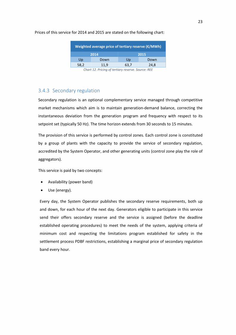
Prices of tertiary reserve, since closer to real time operation, are usually higher than
deviations management. Energy managed on this balancing market in 2014 and 2015 is
shown below:
Energy managed on tertiary reserve (GWh)
2014 2015
Up Down Up Down
3066 1765 3126 1627 Chart 11. Energy managed on tertiary reserve. Source: REE
Chart 10. Tertiary reserve pricing. Source: REE
23
Prices of this service for 2014 and 2015 are stated on the following chart:
Weighted average price of tertiary reserve (€/MWh)
2014 2015
Up Down Up Down
58,2 11,9 63,7 24,8 Chart 12. Pricing of tertiary reserve. Source: REE
3.4.3 Secondary regulation
Secondary regulation is an optional complementary service managed through competitive
market mechanisms which aim is to maintain generation-demand balance, correcting the
instantaneous deviation from the generation program and frequency with respect to its
setpoint set (typically 50 Hz). The time horizon extends from 30 seconds to 15 minutes.
The provision of this service is performed by control zones. Each control zone is constituted
by a group of plants with the capacity to provide the service of secondary regulation,
accredited by the System Operator, and other generating units (control zone play the role of
aggregators).
This service is paid by two concepts:
Availability (power band)
Use (energy).
Every day, the System Operator publishes the secondary reserve requirements, both up
and down, for each hour of the next day. Generators eligible to participate in this service
send their offers secondary reserve and the service is assigned (before the deadline
established operating procedures) to meet the needs of the system, applying criteria of
minimum cost and respecting the limitations program established for safety in the
settlement process PDBF restrictions, establishing a marginal price of secondary regulation
band every hour.
24
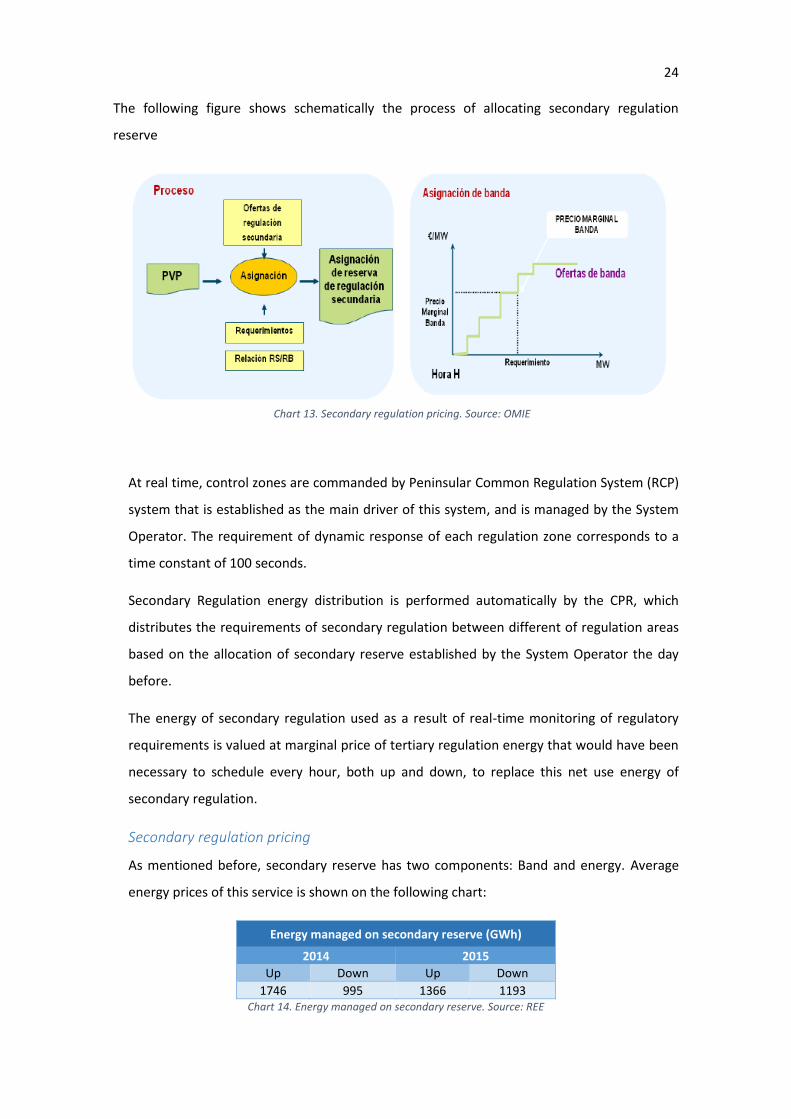
The following figure shows schematically the process of allocating secondary regulation
reserve
At real time, control zones are commanded by Peninsular Common Regulation System (RCP)
system that is established as the main driver of this system, and is managed by the System
Operator. The requirement of dynamic response of each regulation zone corresponds to a
time constant of 100 seconds.
Secondary Regulation energy distribution is performed automatically by the CPR, which
distributes the requirements of secondary regulation between different of regulation areas
based on the allocation of secondary reserve established by the System Operator the day
before.
The energy of secondary regulation used as a result of real-time monitoring of regulatory
requirements is valued at marginal price of tertiary regulation energy that would have been
necessary to schedule every hour, both up and down, to replace this net use energy of
secondary regulation.
Secondary regulation pricing
As mentioned before, secondary reserve has two components: Band and energy. Average
energy prices of this service is shown on the following chart:
Energy managed on secondary reserve (GWh)
2014 2015
Up Down Up Down
1746 995 1366 1193 Chart 14. Energy managed on secondary reserve. Source: REE
Chart 13. Secondary regulation pricing. Source: OMIE
25
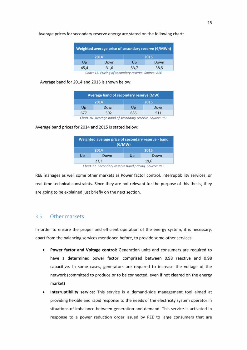
Average prices for secondary reserve energy are stated on the following chart:
Weighted average price of secondary reserve (€/MWh)
2014 2015
Up Down Up Down
45,4 31,6 53,7 38,5 Chart 15. Pricing of secondary reserve. Source: REE
Average band for 2014 and 2015 is shown below:
Average band of secondary reserve (MW)
2014 2015
Up Down Up Down
677 502 685 511 Chart 16. Average band of secondary reserve. Source: REE
Average band prices for 2014 and 2015 is stated below:
Weighted average price of secondary reserve - band (€/MW)
2014 2015
Up Down Up Down
23,3 19,6 Chart 17. Secondary reserve band pricing. Source: REE
REE manages as well some other markets as Power factor control, interruptibility services, or
real time technical constraints. Since they are not relevant for the purpose of this thesis, they
are going to be explained just briefly on the next section.
3.5. Other markets
In order to ensure the proper and efficient operation of the energy system, it is necessary,
apart from the balancing services mentioned before, to provide some other services:
Power factor and Voltage control: Generation units and consumers are required to
have a determined power factor, comprised between 0,98 reactive and 0,98
capacitive. In some cases, generators are required to increase the voltage of the
network (committed to produce or to be connected, even if not cleared on the energy
market)
Interruptibility service: This service is a demand-side management tool aimed at
providing flexible and rapid response to the needs of the electricity system operator in
situations of imbalance between generation and demand. This service is activated in
response to a power reduction order issued by REE to large consumers that are
26
providers of this service, and that are mainly large-scale industry. They are required to
disconnect under some circumstances (high demand episodes, scarcity events… and
compensated economically.
Additional upwards reserve: The aim of this service is to provide additional upwards
power in case of a sharp increase of the demand
Real time technical constraints: Some consumers or generators may be required to be
connected or disconnected if some node of the system suffers a congestion.
3.6. Final Program (P48)
This program is established at the end of the daily scheduling horizon. It contains all energy
programs: those resulting from the Daily Base Operating Program (PDBF); those resulting from
the different sessions of the intraday markets, i.e, the final hourly schedule (PHF), program
modifications associated with the processes of technical constraints and the involvement of
different services units in secondary, tertiary regulation and deviation management process.
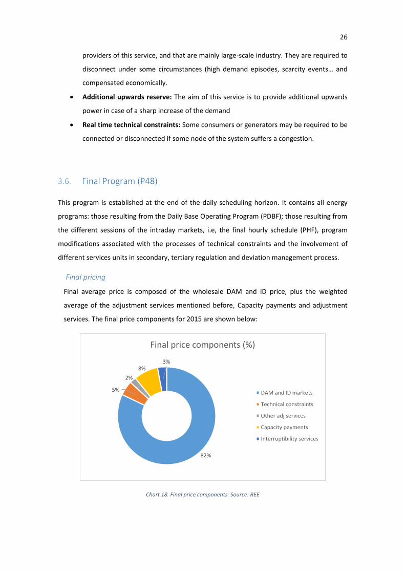
Final pricing
Final average price is composed of the wholesale DAM and ID price, plus the weighted
average of the adjustment services mentioned before, Capacity payments and adjustment
services. The final price components for 2015 are shown below:
Chart 18. Final price components. Source: REE
82%
5%
2%
8%3%
Final price components (%)
DAM and ID markets
Technical constraints
Other adj services
Capacity payments
Interruptibility services


27
4. Deviations
Deviations are stated as the difference between the energy measured at generation plants
busbars (real production) and energy scheduled in different markets established production in
the final program. Deviations may be due to an excess in generation (deviation up) or to a lack
of generation (deviation down) generally:
𝐷𝐸𝑉𝑢 = 𝑀𝐵𝐶𝑢-𝑃𝐻𝐿𝑢
where:
𝑀𝐵𝐶𝑢: Energy measured at busbars of each production / acquisition unit.
𝑃𝐻𝐿𝑢: Final program of the production / acquisition unit.
Deviations are usually caused by failures in the primary resource forecast as is the case of
renewable technologies, or unforeseen outages that could affect thermal units. Demand
forecast error may induce to an error on the acquisition units.
When they occur, deviations cause a mismatch in the system that has to be corrected by the
call for balancing markets by the System Operator. Deviations have an associated cost which
can generate a collection right or an obligation to pay, depending on the system requirements.
This cost should be paid by causing agents and is determined both for the “up” and “down”
energy by the following criteria:
System needs
“up”
System needs
“down”
DEV > 0 DAM
Min (DAM,
WAPEU)
DEV < 0 Max (DAM,
WAPED) DAM
Chart 19. Deviations pricing
Where:
DAM Daily Market Price
WAPED weighted average price per unit of energy for the system to go down,
including Deviations Management, Tertiary Regulation and Secondary Regulation
28
WAPEU weighted average price per unit of energy for the system to go up, including
Deviations Management, Tertiary Regulation and Secondary Regulation
From the upper chart we can derive that the deviations that favor the system needs are for
free, they receive or they have to pay the same amount of money that would have resulted
from the DAM operation. On the other hand, If the deviation goes against the system
requirements, the corresponding unit will incur on a loss.
Let us introduce an example, extracted from the market data published by OMIE and REE:
Date Month Hour DAM Payment
deviations down
Collection deviations
up
System Requirements
J 01 January 8 36,22 37,8 36,22 up
J 01 January 10 36,6 36,6 21,65 down
Chart 20. Example of deviations pricing
The upper chart shows the DAM price and the payment/collection price for deviations
up/down. As can be appreciated, when the system needs energy (requirements up), the DAM
coincides with the payment for deviations up. On the other hand, if the system has plenty of
energy (requirements down), the unit that deviates down is the one which losses nothing.
On the first case, if a unit incurs on a deviation up, she losses nothing, as the payment for
deviations down (36,22€/MWh) is the same as the DAM price (36,22€/MWh). On the contrary,
if the deviation is down, that unit would have to pay 37,8 €/MWh so she losses 37,8-36,22 =
1,58 €/MWh of deviation.
On the second one, if a unit incurs on a deviation down, she losses nothing, as the DAM price
(36,6€/MWh) coincides with the payment for deviations down (36,6€/MWh). However, if the
deviation is up, she losses 36,6-21,65 = 14,95 €/MWh.
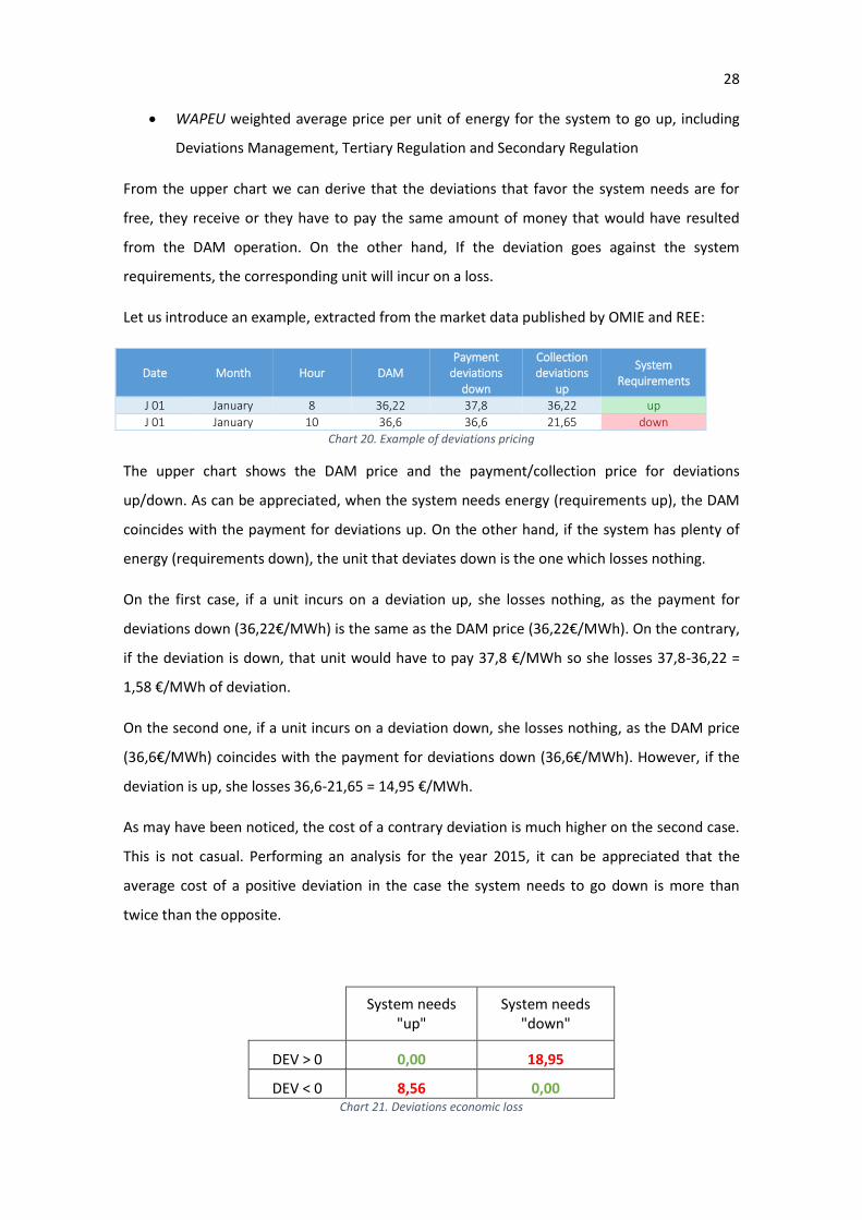
As may have been noticed, the cost of a contrary deviation is much higher on the second case.
This is not casual. Performing an analysis for the year 2015, it can be appreciated that the
average cost of a positive deviation in the case the system needs to go down is more than
twice than the opposite.
System needs "up"
System needs "down"
DEV > 0 0,00 18,95
DEV < 0 8,56 0,00 Chart 21. Deviations economic loss
29
This fact may be crucial in case of developing a strategy. When, as an example, the wind
forecast is not clear, it should be less “harmful” to plan the commitment of the unit in order to
have a slight deviation down (schedule more than the expected production) However, in the
thermal plants case, since we are studying thermal outages, which are always deviations down,
it has no further importance.
It should be noticed that those deviation cost are always calculated in comparison with the
DAM price, which is stated as the reference. Intraday markets allow more negotiations, and
the price is usually slightly different than the DAM. With that on mind, it is possible to make
money with a deviation (if the ID price is higher than the deviation cost). This will be explained
on further chapters.
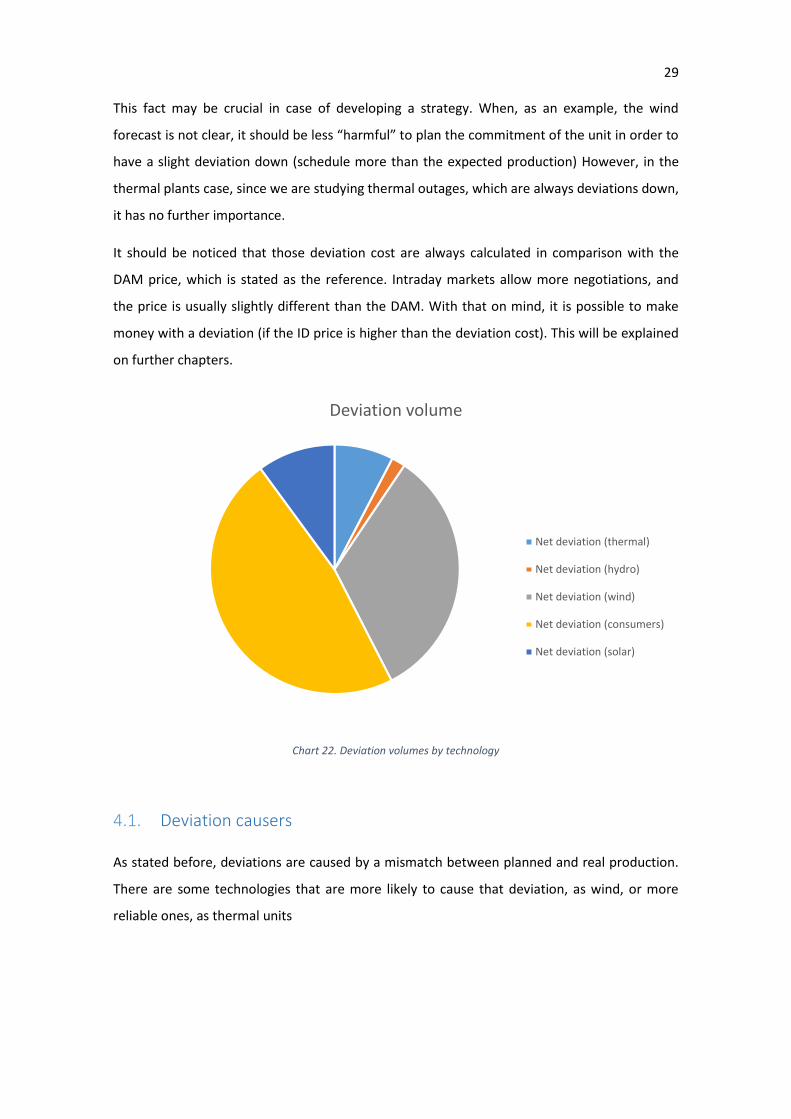
Chart 22. Deviation volumes by technology
4.1. Deviation causers
As stated before, deviations are caused by a mismatch between planned and real production.
There are some technologies that are more likely to cause that deviation, as wind, or more
reliable ones, as thermal units
Deviation volume
Net deviation (thermal)
Net deviation (hydro)
Net deviation (wind)
Net deviation (consumers)
Net deviation (solar)
30
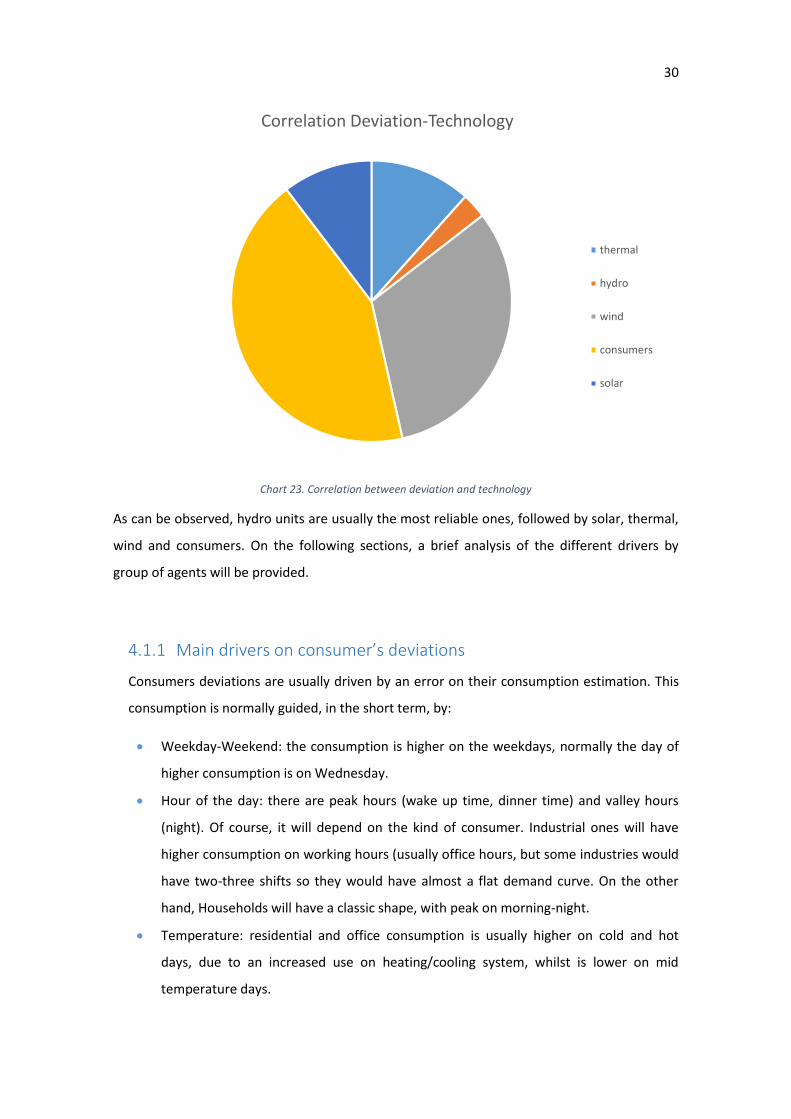
Chart 23. Correlation between deviation and technology
As can be observed, hydro units are usually the most reliable ones, followed by solar, thermal,
wind and consumers. On the following sections, a brief analysis of the different drivers by
group of agents will be provided.
4.1.1 Main drivers on consumer’s deviations
Consumers deviations are usually driven by an error on their consumption estimation. This
consumption is normally guided, in the short term, by:
Weekday-Weekend: the consumption is higher on the weekdays, normally the day of
higher consumption is on Wednesday.
Hour of the day: there are peak hours (wake up time, dinner time) and valley hours
(night). Of course, it will depend on the kind of consumer. Industrial ones will have
higher consumption on working hours (usually office hours, but some industries would
have two-three shifts so they would have almost a flat demand curve. On the other
hand, Households will have a classic shape, with peak on morning-night.
Temperature: residential and office consumption is usually higher on cold and hot
days, due to an increased use on heating/cooling system, whilst is lower on mid
temperature days.
Correlation Deviation-Technology
thermal
hydro
wind
consumers
solar
31
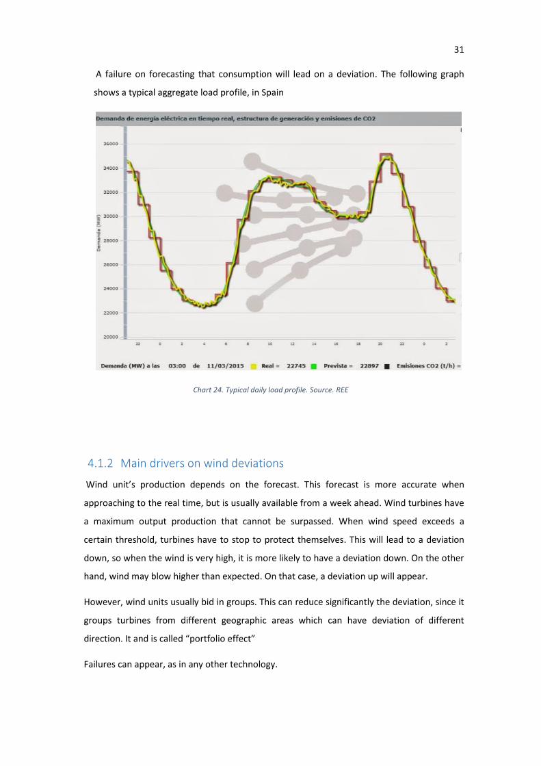
A failure on forecasting that consumption will lead on a deviation. The following graph
shows a typical aggregate load profile, in Spain
Chart 24. Typical daily load profile. Source. REE
4.1.2 Main drivers on wind deviations
Wind unit’s production depends on the forecast. This forecast is more accurate when
approaching to the real time, but is usually available from a week ahead. Wind turbines have
a maximum output production that cannot be surpassed. When wind speed exceeds a
certain threshold, turbines have to stop to protect themselves. This will lead to a deviation
down, so when the wind is very high, it is more likely to have a deviation down. On the other
hand, wind may blow higher than expected. On that case, a deviation up will appear.
However, wind units usually bid in groups. This can reduce significantly the deviation, since it
groups turbines from different geographic areas which can have deviation of different
direction. It and is called “portfolio effect”
Failures can appear, as in any other technology.

32
4.1.3 Main drivers on solar deviations
Solar units depend as well on the forecast. But also have a big seasonality. Winter days, with
less sun hours, will lead to a decreased production, and summer days, which are longer, will
lead to a higher production. However, this fact does not lead to uncertainty. On the short
term, solar production depends on the forecast: cloudy days will lead to a decrease on the
production.

33
5. Classification of ID operations
In order to assess the expected operations on the new Intraday schedule, it is necessary to
classify the ID operations. Depending on the assumed purpose of the transactions, those will
be classified and then quantified by volume and number of operations. After that, an
estimation on the increase of each type of operation will be performed and, as a result, the
expected volume under de new schedule will be obtained
5.1 Agents behavior
Unexpected outages affect thermal units on different ways. In order to assess the impact of
the increased Intraday sessions, a classification is needed:
If they notice the problem after the negotiation time and have no time to reschedule
If they notice the problem and have time to reschedule on the next ID
If they notice that they no longer have the problem and can commit the available
power on the next ID
A speculative behavior
If they expect the problem to be fixed at certain time and finally it is not possible and
they incur on a deviation
If there is no deviation
A detailed description of each case will be provided below
5.1.1 No time to renegotiate
Outages, as will be justified on later chapters, are assumed equally distributed along the
day. They may happen before the negotiating time for the next Intraday session, during or
after. If it happens on the two first cases, the reschedule will be applied on the next ID
session, with a waiting time (at which units will have to pay deviations) that depends on the
session and it is shown below
34
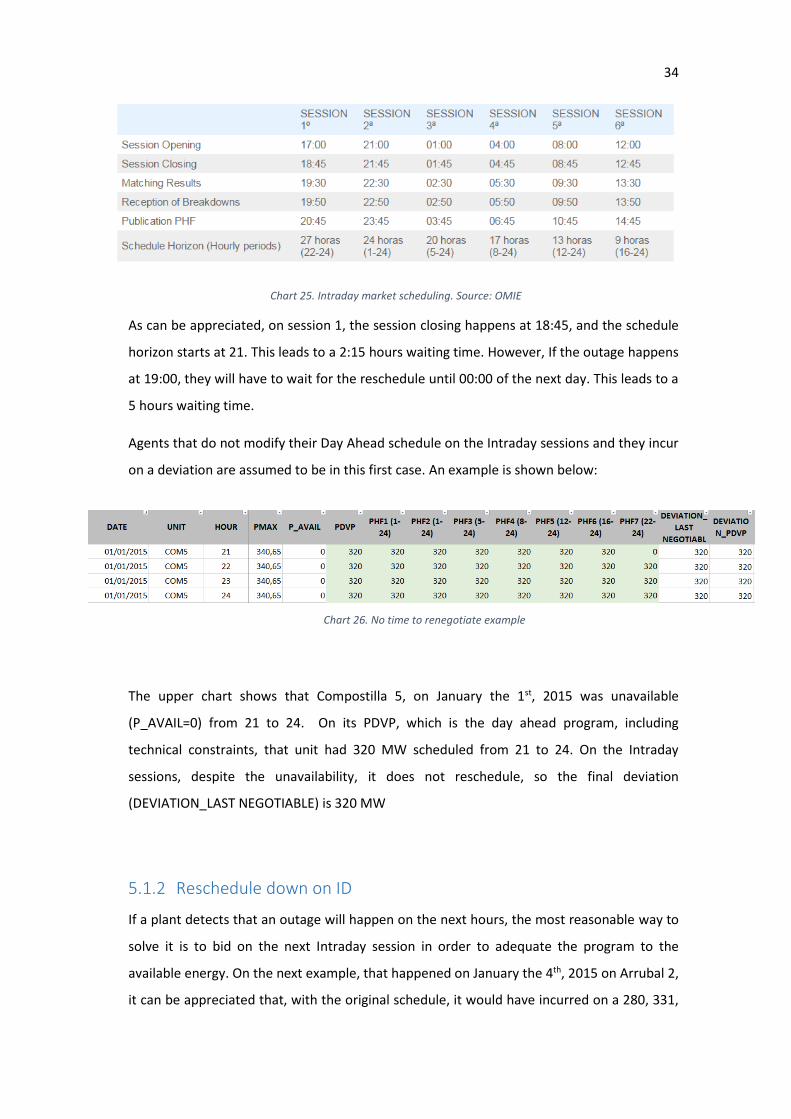
Chart 25. Intraday market scheduling. Source: OMIE
As can be appreciated, on session 1, the session closing happens at 18:45, and the schedule
horizon starts at 21. This leads to a 2:15 hours waiting time. However, If the outage happens
at 19:00, they will have to wait for the reschedule until 00:00 of the next day. This leads to a
5 hours waiting time.
Agents that do not modify their Day Ahead schedule on the Intraday sessions and they incur
on a deviation are assumed to be in this first case. An example is shown below:
The upper chart shows that Compostilla 5, on January the 1st, 2015 was unavailable
(P_AVAIL=0) from 21 to 24. On its PDVP, which is the day ahead program, including
technical constraints, that unit had 320 MW scheduled from 21 to 24. On the Intraday
sessions, despite the unavailability, it does not reschedule, so the final deviation
(DEVIATION_LAST NEGOTIABLE) is 320 MW
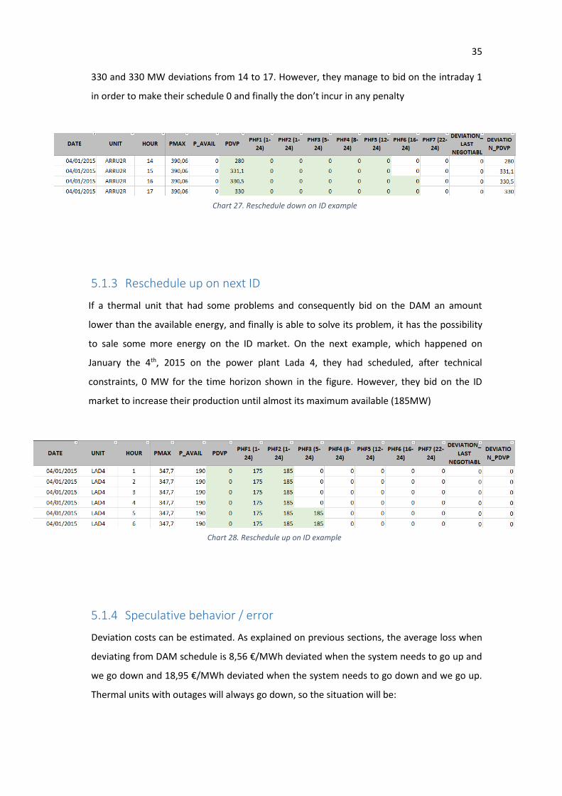
5.1.2 Reschedule down on ID
If a plant detects that an outage will happen on the next hours, the most reasonable way to
solve it is to bid on the next Intraday session in order to adequate the program to the
available energy. On the next example, that happened on January the 4th, 2015 on Arrubal 2,
it can be appreciated that, with the original schedule, it would have incurred on a 280, 331,
Chart 26. No time to renegotiate example
35
330 and 330 MW deviations from 14 to 17. However, they manage to bid on the intraday 1
in order to make their schedule 0 and finally the don’t incur in any penalty
5.1.3 Reschedule up on next ID
If a thermal unit that had some problems and consequently bid on the DAM an amount
lower than the available energy, and finally is able to solve its problem, it has the possibility
to sale some more energy on the ID market. On the next example, which happened on
January the 4th, 2015 on the power plant Lada 4, they had scheduled, after technical
constraints, 0 MW for the time horizon shown in the figure. However, they bid on the ID
market to increase their production until almost its maximum available (185MW)
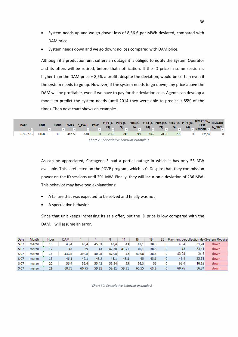
5.1.4 Speculative behavior / error
Deviation costs can be estimated. As explained on previous sections, the average loss when
deviating from DAM schedule is 8,56 €/MWh deviated when the system needs to go up and
we go down and 18,95 €/MWh deviated when the system needs to go down and we go up.
Thermal units with outages will always go down, so the situation will be:
Chart 27. Reschedule down on ID example
Chart 28. Reschedule up on ID example
36
System needs up and we go down: loss of 8,56 € per MWh deviated, compared with
DAM price
System needs down and we go down: no loss compared with DAM price.
Although if a production unit suffers an outage it is obliged to notify the System Operator
and its offers will be retired, before that notification, If the ID price in some session is
higher than the DAM price + 8,56, a profit, despite the deviation, would be certain even if
the system needs to go up. However, if the system needs to go down, any price above the
DAM will be profitable, even if we have to pay for the deviation cost. Agents can develop a
model to predict the system needs (until 2014 they were able to predict it 85% of the
time). Then next chart shows an example:
As can be appreciated, Cartagena 3 had a partial outage in which it has only 55 MW
available. This is reflected on the PDVP program, which is 0. Despite that, they commission
power on the ID sessions until 291 MW. Finally, they will incur on a deviation of 236 MW.
This behavior may have two explanations:
A failure that was expected to be solved and finally was not
A speculative behavior
Since that unit keeps increasing its sale offer, but the ID price is low compared with the
DAM, I will assume an error.
Chart 29. Speculative behavior example 1
Chart 30. Speculative behavior example 2
37
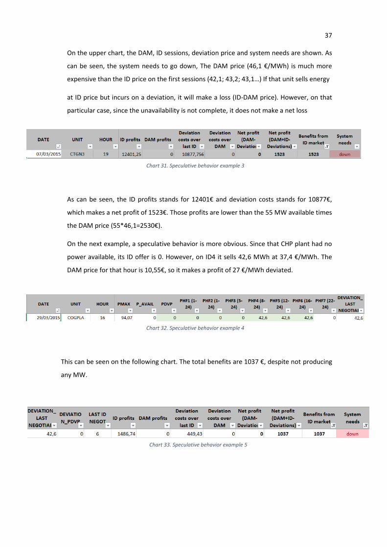
On the upper chart, the DAM, ID sessions, deviation price and system needs are shown. As
can be seen, the system needs to go down, The DAM price (46,1 €/MWh) is much more
expensive than the ID price on the first sessions (42,1; 43,2; 43,1…) If that unit sells energy
at ID price but incurs on a deviation, it will make a loss (ID-DAM price). However, on that
particular case, since the unavailability is not complete, it does not make a net loss
As can be seen, the ID profits stands for 12401€ and deviation costs stands for 10877€,
which makes a net profit of 1523€. Those profits are lower than the 55 MW available times
the DAM price (55*46,1=2530€).
On the next example, a speculative behavior is more obvious. Since that CHP plant had no
power available, its ID offer is 0. However, on ID4 it sells 42,6 MWh at 37,4 €/MWh. The
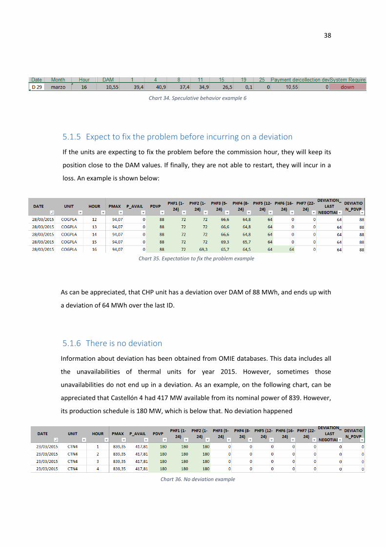
DAM price for that hour is 10,55€, so it makes a profit of 27 €/MWh deviated.
This can be seen on the following chart. The total benefits are 1037 €, despite not producing
any MW.
Chart 31. Speculative behavior example 3
Chart 32. Speculative behavior example 4
Chart 33. Speculative behavior example 5
38
5.1.5 Expect to fix the problem before incurring on a deviation
If the units are expecting to fix the problem before the commission hour, they will keep its
position close to the DAM values. If finally, they are not able to restart, they will incur in a
loss. An example is shown below:
As can be appreciated, that CHP unit has a deviation over DAM of 88 MWh, and ends up with
a deviation of 64 MWh over the last ID.
5.1.6 There is no deviation
Information about deviation has been obtained from OMIE databases. This data includes all
the unavailabilities of thermal units for year 2015. However, sometimes those
unavailabilities do not end up in a deviation. As an example, on the following chart, can be
appreciated that Castellón 4 had 417 MW available from its nominal power of 839. However,
its production schedule is 180 MW, which is below that. No deviation happened
Chart 34. Speculative behavior example 6
Chart 35. Expectation to fix the problem example
Chart 36. No deviation example
39
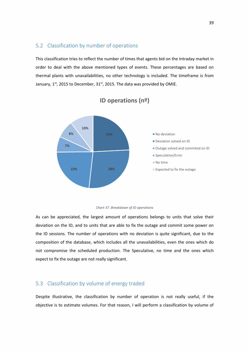
5.2 Classification by number of operations
This classification tries to reflect the number of times that agents bid on the Intraday market in
order to deal with the above mentioned types of events. These percentages are based on
thermal plants with unavailabilities, no other technology is included. The timeframe is from
January, 1st, 2015 to December, 31st, 2015. The data was provided by OMIE.
Chart 37. Breakdown of ID operations
As can be appreciated, the largest amount of operations belongs to units that solve their
deviation on the ID, and to units that are able to fix the outage and commit some power on
the ID sessions. The number of operations with no deviation is quite significant, due to the
composition of the database, which includes all the unavailabilities, even the ones which do
not compromise the scheduled production. The Speculative, no time and the ones which
expect to fix the outage are not really significant.
5.3 Classification by volume of energy traded
Despite illustrative, the classification by number of operation is not really useful, if the
objective is to estimate volumes. For that reason, I will perform a classification by volume of
24%
28%23%
7%
8%
10%
ID operations (nº)
No deviation
Deviation solved on ID
Outage solved and commited on ID
Speculative/Error
No time
Expected to fix the outage
40
energy traded. There will be a separation, in order to separate energies negotiated to increase
the production and the ones negotiated to decrease it.
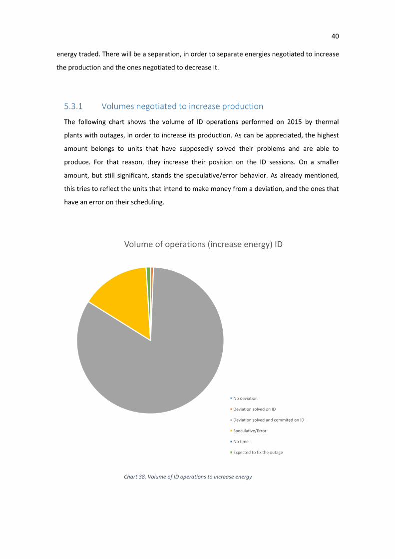
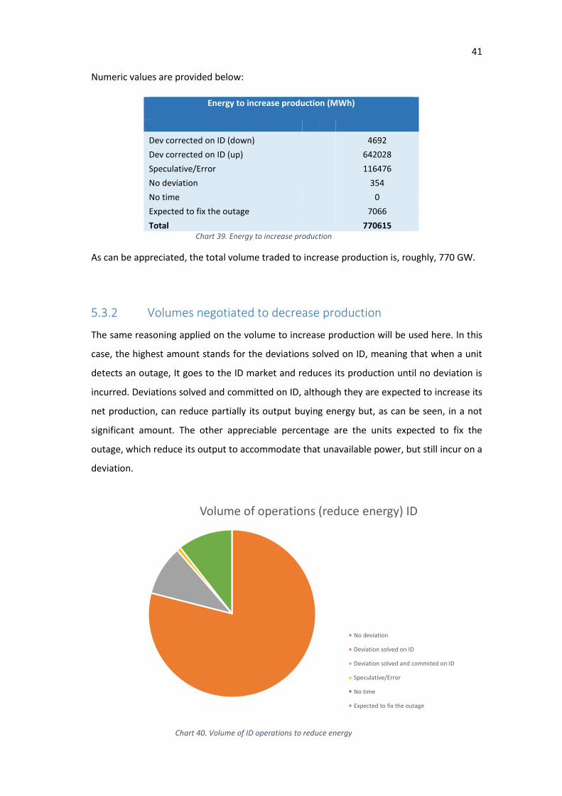
5.3.1 Volumes negotiated to increase production
The following chart shows the volume of ID operations performed on 2015 by thermal
plants with outages, in order to increase its production. As can be appreciated, the highest
amount belongs to units that have supposedly solved their problems and are able to
produce. For that reason, they increase their position on the ID sessions. On a smaller
amount, but still significant, stands the speculative/error behavior. As already mentioned,
this tries to reflect the units that intend to make money from a deviation, and the ones that
have an error on their scheduling.
Volume of operations (increase energy) ID
No deviation
Deviation solved on ID
Deviation solved and commited on ID
Speculative/Error
No time
Expected to fix the outage
Chart 38. Volume of ID operations to increase energy
41
Numeric values are provided below:
As can be appreciated, the total volume traded to increase production is, roughly, 770 GW.
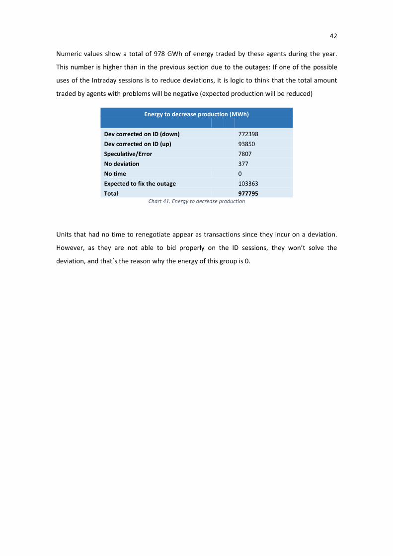
5.3.2 Volumes negotiated to decrease production
The same reasoning applied on the volume to increase production will be used here. In this
case, the highest amount stands for the deviations solved on ID, meaning that when a unit
detects an outage, It goes to the ID market and reduces its production until no deviation is
incurred. Deviations solved and committed on ID, although they are expected to increase its
net production, can reduce partially its output buying energy but, as can be seen, in a not
significant amount. The other appreciable percentage are the units expected to fix the
outage, which reduce its output to accommodate that unavailable power, but still incur on a
deviation.
Energy to increase production (MWh)
Dev corrected on ID (down) 4692
Dev corrected on ID (up) 642028
Speculative/Error 116476
No deviation 354
No time 0
Expected to fix the outage 7066
Total 770615 Chart 39. Energy to increase production
Volume of operations (reduce energy) ID
No deviation
Deviation solved on ID
Deviation solved and commited on ID
Speculative/Error
No time
Expected to fix the outage
Chart 40. Volume of ID operations to reduce energy
42
Numeric values show a total of 978 GWh of energy traded by these agents during the year.
This number is higher than in the previous section due to the outages: If one of the possible
uses of the Intraday sessions is to reduce deviations, it is logic to think that the total amount
traded by agents with problems will be negative (expected production will be reduced)
Energy to decrease production (MWh)
Dev corrected on ID (down) 772398
Dev corrected on ID (up) 93850
Speculative/Error
7807
No deviation
377
No time
0
Expected to fix the outage 103363
Total
977795 Chart 41. Energy to decrease production
Units that had no time to renegotiate appear as transactions since they incur on a deviation.
However, as they are not able to bid properly on the ID sessions, they won’t solve the
deviation, and that´s the reason why the energy of this group is 0.
43
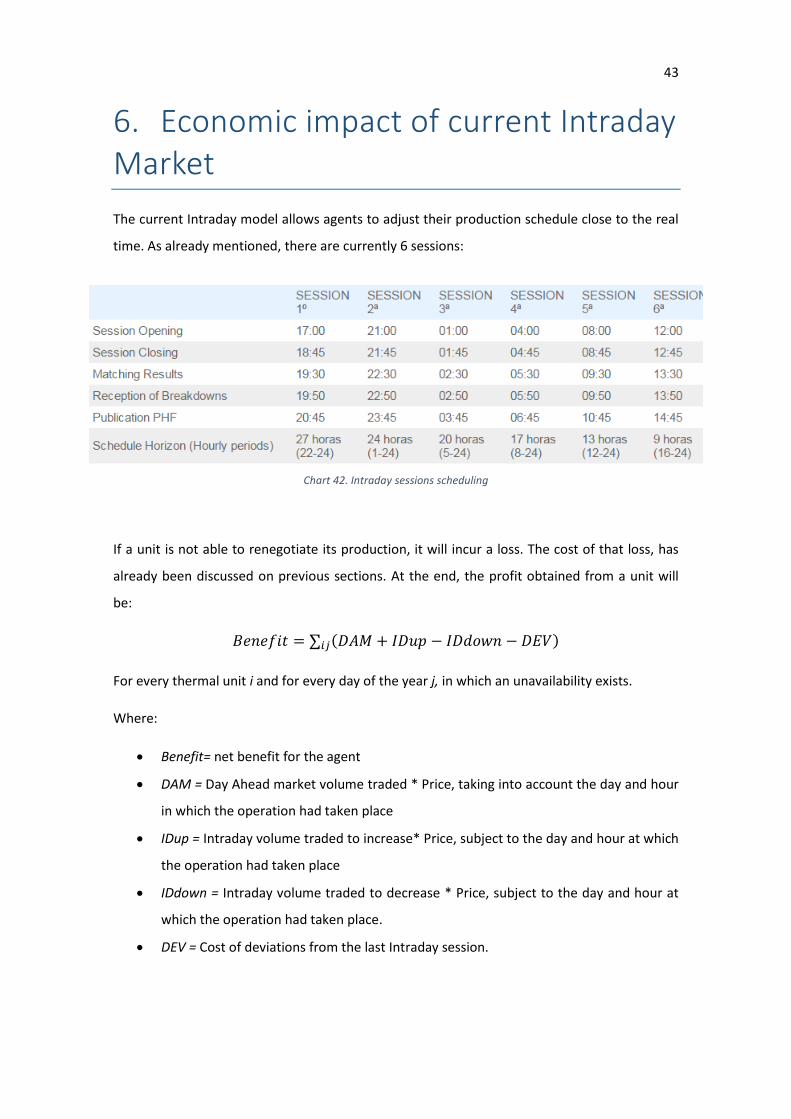
6. Economic impact of current Intraday Market
The current Intraday model allows agents to adjust their production schedule close to the real
time. As already mentioned, there are currently 6 sessions:
If a unit is not able to renegotiate its production, it will incur a loss. The cost of that loss, has
already been discussed on previous sections. At the end, the profit obtained from a unit will
be:
𝐵𝑒𝑛𝑒𝑓𝑖𝑡 = ∑𝑖𝑗(𝐷𝐴𝑀 + 𝐼𝐷𝑢𝑝 − 𝐼𝐷𝑑𝑜𝑤𝑛 − 𝐷𝐸𝑉)
For every thermal unit i and for every day of the year j, in which an unavailability exists.
Where:
Benefit= net benefit for the agent
DAM = Day Ahead market volume traded * Price, taking into account the day and hour
in which the operation had taken place
IDup = Intraday volume traded to increase* Price, subject to the day and hour at which
the operation had taken place
IDdown = Intraday volume traded to decrease * Price, subject to the day and hour at
which the operation had taken place.
DEV = Cost of deviations from the last Intraday session.
Chart 42. Intraday sessions scheduling
44
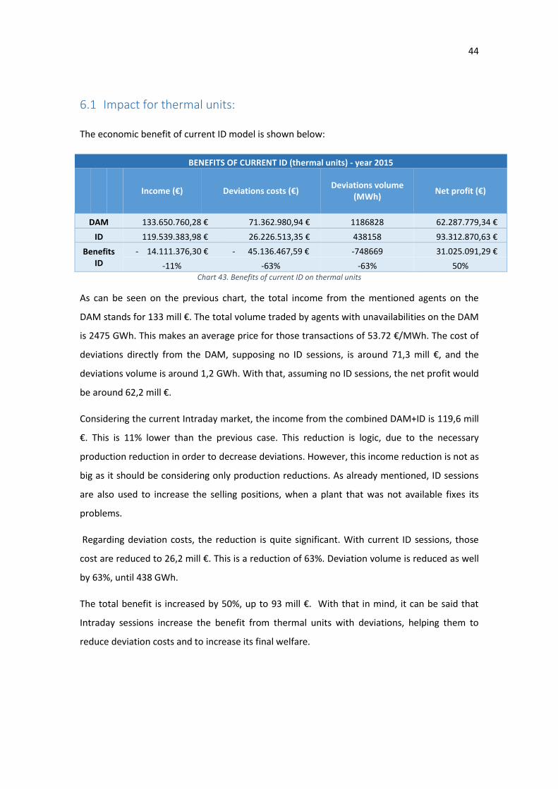
6.1 Impact for thermal units:
The economic benefit of current ID model is shown below:
BENEFITS OF CURRENT ID (thermal units) - year 2015
Income (€) Deviations costs (€) Deviations volume
(MWh) Net profit (€)
DAM 133.650.760,28 € 71.362.980,94 € 1186828 62.287.779,34 €
ID 119.539.383,98 € 26.226.513,35 € 438158 93.312.870,63 €
Benefits ID
- 14.111.376,30 € - 45.136.467,59 € -748669 31.025.091,29 €
-11% -63% -63% 50% Chart 43. Benefits of current ID on thermal units
As can be seen on the previous chart, the total income from the mentioned agents on the
DAM stands for 133 mill €. The total volume traded by agents with unavailabilities on the DAM
is 2475 GWh. This makes an average price for those transactions of 53.72 €/MWh. The cost of
deviations directly from the DAM, supposing no ID sessions, is around 71,3 mill €, and the
deviations volume is around 1,2 GWh. With that, assuming no ID sessions, the net profit would
be around 62,2 mill €.
Considering the current Intraday market, the income from the combined DAM+ID is 119,6 mill
€. This is 11% lower than the previous case. This reduction is logic, due to the necessary
production reduction in order to decrease deviations. However, this income reduction is not as
big as it should be considering only production reductions. As already mentioned, ID sessions
are also used to increase the selling positions, when a plant that was not available fixes its
problems.
Regarding deviation costs, the reduction is quite significant. With current ID sessions, those
cost are reduced to 26,2 mill €. This is a reduction of 63%. Deviation volume is reduced as well
by 63%, until 438 GWh.
The total benefit is increased by 50%, up to 93 mill €. With that in mind, it can be said that
Intraday sessions increase the benefit from thermal units with deviations, helping them to
reduce deviation costs and to increase its final welfare.
45
7. Design of the new Intraday Market
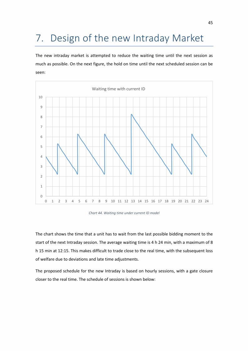
The new intraday market is attempted to reduce the waiting time until the next session as
much as possible. On the next figure, the hold on time until the next scheduled session can be
seen:
Chart 44. Waiting time under current ID model
The chart shows the time that a unit has to wait from the last possible bidding moment to the
start of the next Intraday session. The average waiting time is 4 h 24 min, with a maximum of 8
h 15 min at 12:15. This makes difficult to trade close to the real time, with the subsequent loss
of welfare due to deviations and late time adjustments.
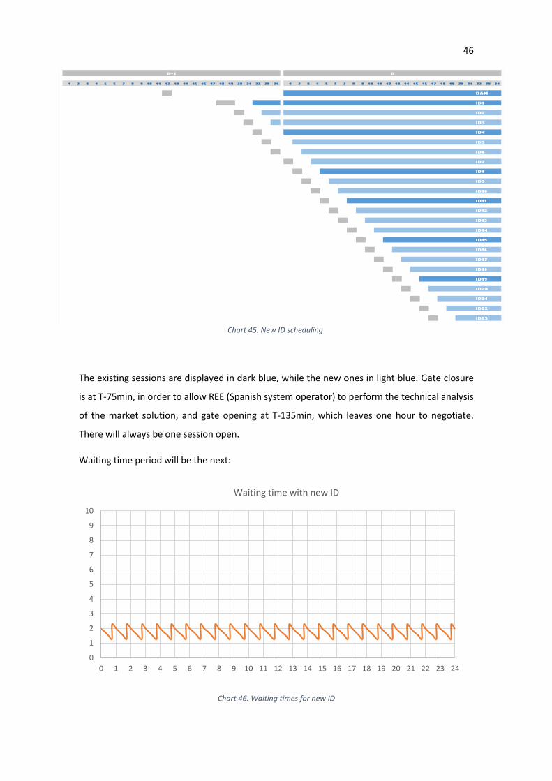
The proposed schedule for the new Intraday is based on hourly sessions, with a gate closure
closer to the real time. The schedule of sessions is shown below:
0
1
2
3
4
5
6
7
8
9
10
0 1 2 3 4 5 6 7 8 9 10 11 12 13 14 15 16 17 18 19 20 21 22 23 24
Waiting time with current ID
46
The existing sessions are displayed in dark blue, while the new ones in light blue. Gate closure
is at T-75min, in order to allow REE (Spanish system operator) to perform the technical analysis
of the market solution, and gate opening at T-135min, which leaves one hour to negotiate.
There will always be one session open.
Waiting time period will be the next:
Chart 46. Waiting times for new ID
0
1
2
3
4
5
6
7
8
9
10
0 1 2 3 4 5 6 7 8 9 10 11 12 13 14 15 16 17 18 19 20 21 22 23 24
Waiting time with new ID
Chart 45. New ID scheduling
47
As can be appreciated, the waiting time has been reduced drastically. Now, the average is 1 h
45 min, which is 2 h 40 min lower than on the original case. This will allow an operation much
closer to the real time, reducing deviations and increasing the benefits for the agents.
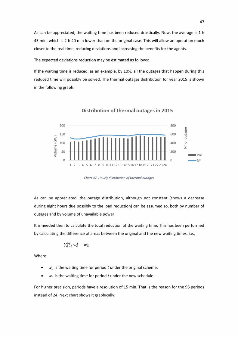
The expected deviations reduction may be estimated as follows:
If the waiting time is reduced, as an example, by 10%, all the outages that happen during this
reduced time will possibly be solved. The thermal outages distribution for year 2015 is shown
in the following graph:
Chart 47. Hourly distribution of thermal outages
As can be appreciated, the outage distribution, although not constant (shows a decrease
during night hours due possibly to the load reduction) can be assumed so, both by number of
outages and by volume of unavailable power.
It is needed then to calculate the total reduction of the waiting time. This has been performed
by calculating the difference of areas between the original and the new waiting times. i.e.,
∑ 𝑤𝑜𝑡 − 𝑤𝑛
𝑡96𝑡=1
Where:
𝑤𝑜 is the waiting time for period t under the original scheme.
𝑤𝑛 is the waiting time for period t under the new schedule.
For higher precision, periods have a resolution of 15 min. That is the reason for the 96 periods
instead of 24. Next chart shows it graphically:
0
200
400
600
800
0
50
100
150
200
1 2 3 4 5 6 7 8 9 10 11 12 13 14 15 16 17 18 19 20 21 22 23 24
Nº
of
ou
tage
s
Vo
lum
e (G
W)
Distribution of thermal outages in 2015
Vol
Nº
48
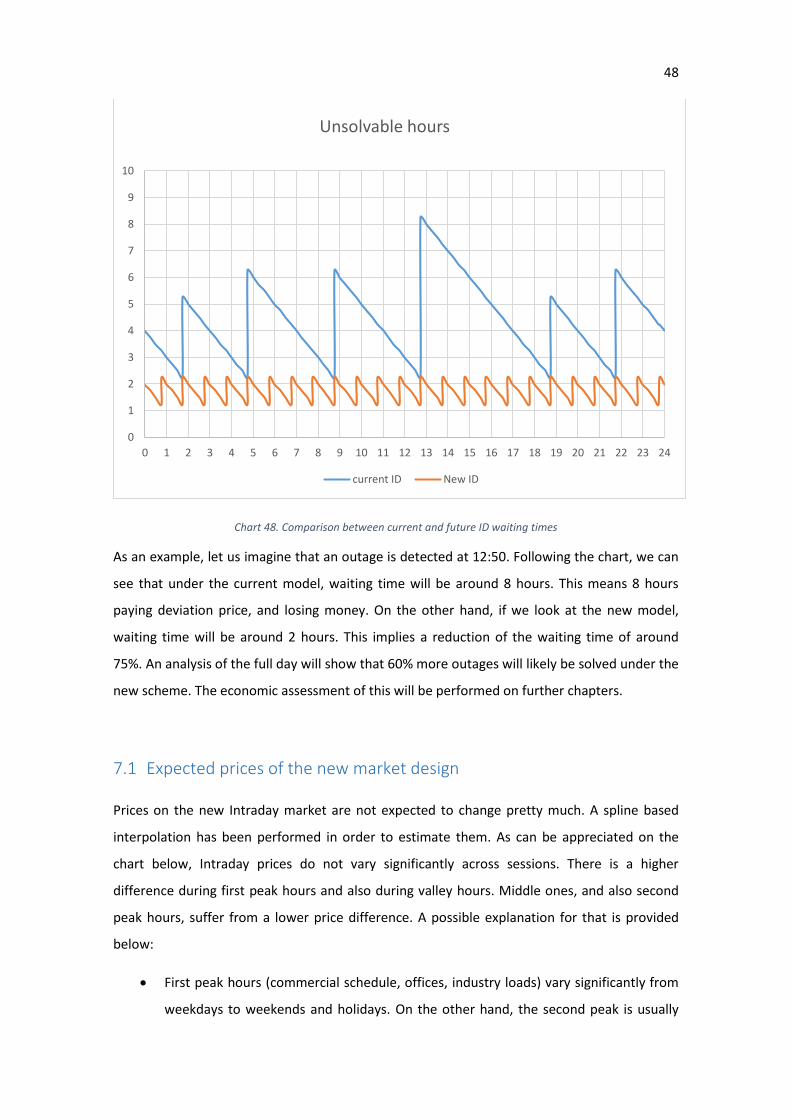
Chart 48. Comparison between current and future ID waiting times
As an example, let us imagine that an outage is detected at 12:50. Following the chart, we can
see that under the current model, waiting time will be around 8 hours. This means 8 hours
paying deviation price, and losing money. On the other hand, if we look at the new model,
waiting time will be around 2 hours. This implies a reduction of the waiting time of around
75%. An analysis of the full day will show that 60% more outages will likely be solved under the
new scheme. The economic assessment of this will be performed on further chapters.
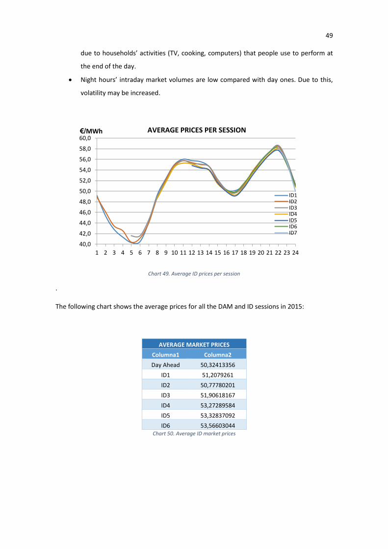
7.1 Expected prices of the new market design
Prices on the new Intraday market are not expected to change pretty much. A spline based
interpolation has been performed in order to estimate them. As can be appreciated on the
chart below, Intraday prices do not vary significantly across sessions. There is a higher
difference during first peak hours and also during valley hours. Middle ones, and also second
peak hours, suffer from a lower price difference. A possible explanation for that is provided
below:
First peak hours (commercial schedule, offices, industry loads) vary significantly from
weekdays to weekends and holidays. On the other hand, the second peak is usually
0
1
2
3
4
5
6
7
8
9
10
0 1 2 3 4 5 6 7 8 9 10 11 12 13 14 15 16 17 18 19 20 21 22 23 24
Unsolvable hours
current ID New ID
49
due to households’ activities (TV, cooking, computers) that people use to perform at
the end of the day.
Night hours’ intraday market volumes are low compared with day ones. Due to this,
volatility may be increased.
Chart 49. Average ID prices per session
.
The following chart shows the average prices for all the DAM and ID sessions in 2015:
AVERAGE MARKET PRICES
Columna1 Columna2
Day Ahead 50,32413356
ID1 51,2079261
ID2 50,77780201
ID3 51,90618167
ID4 53,27289584
ID5 53,32837092
ID6 53,56603044 Chart 50. Average ID market prices
40,0
42,0
44,0
46,0
48,0
50,0
52,0
54,0
56,0
58,0
60,0
1 2 3 4 5 6 7 8 9 10 11 12 13 14 15 16 17 18 19 20 21 22 23 24
ID1ID2ID3ID4ID5ID6ID7
AVERAGE PRICES PER SESSION€/MWh
50
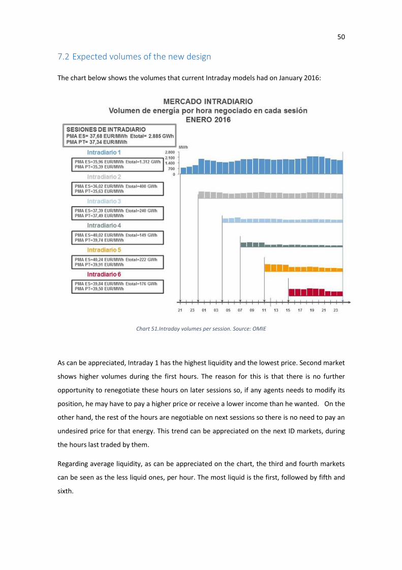
7.2 Expected volumes of the new design
The chart below shows the volumes that current Intraday models had on January 2016:
Chart 51.Intraday volumes per session. Source: OMIE
As can be appreciated, Intraday 1 has the highest liquidity and the lowest price. Second market
shows higher volumes during the first hours. The reason for this is that there is no further
opportunity to renegotiate these hours on later sessions so, if any agents needs to modify its
position, he may have to pay a higher price or receive a lower income than he wanted. On the
other hand, the rest of the hours are negotiable on next sessions so there is no need to pay an
undesired price for that energy. This trend can be appreciated on the next ID markets, during
the hours last traded by them.
Regarding average liquidity, as can be appreciated on the chart, the third and fourth markets
can be seen as the less liquid ones, per hour. The most liquid is the first, followed by fifth and
sixth.

51
Volumes under the new model are expected to suffer a higher impact. To asses that, it is
necessary to discriminate between the different types of operations performed under the
current scheme. The types of operations were already explained. The expected variation will
be:
For deviations corrected up, an increase of 60 %. The reason for that increase is that
these units’ will be able to operate much closer to real time. Due to that, as explained
previously 60% more solved outages will be detected on time to bid and produce on
the next ID session
For deviations corrected down, an increase of 60 % is expected. The reasons for that
are the same as in the previous point but applied to deviations reduction.
For Speculative behavior, no increase expected. This may not be accurate, as the
agents will surely try to get advantage of the new markets in order to make some
profit. However, as it is very difficult to assess that, we preferred to assume no
increase than to provide a non-founded value.
For no deviation, no increase expected. This kind of behavior, as mentioned before,
was included on the database due to an unavailability declared by the agents, but this,
as was lower than the program, didn´t lead to any deviation.
For the units that were expecting to fix the outage, no increase expected. Since they
were expecting to fix the problem and produce normally without deviation, no further
correction is expected. However, some of them, if they notice the impossibility to
solve the problem, would surely bid on the last session possible to adequate its
production.
For the reasons provided above, and some others provided later on, the economic assessment
of the new market has to be treated as orientative.

52
8. Economic analysis of new Intraday Market
New sessions, as mentioned before, will allow agents to bid closer to real time. This will cause
an impact on their deviations and, consequently, to its profit. The impact to each individual
agent will be difficult to assess. For this reason, a joint analysis has been performed, studying
the variation of the deviations price, deviations volume and Intraday operations. Each of the
parts will be explained individually.
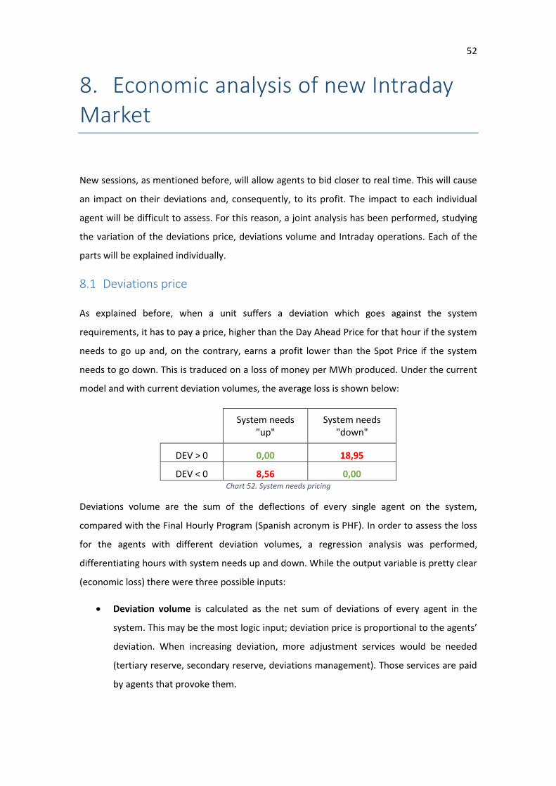
8.1 Deviations price
As explained before, when a unit suffers a deviation which goes against the system
requirements, it has to pay a price, higher than the Day Ahead Price for that hour if the system
needs to go up and, on the contrary, earns a profit lower than the Spot Price if the system
needs to go down. This is traduced on a loss of money per MWh produced. Under the current
model and with current deviation volumes, the average loss is shown below:
System needs "up"
System needs "down"
DEV > 0 0,00 18,95
DEV < 0 8,56 0,00 Chart 52. System needs pricing
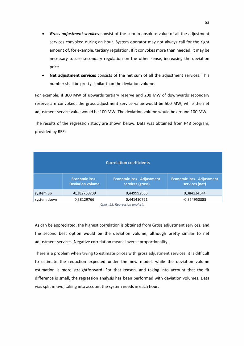
Deviations volume are the sum of the deflections of every single agent on the system,
compared with the Final Hourly Program (Spanish acronym is PHF). In order to assess the loss
for the agents with different deviation volumes, a regression analysis was performed,
differentiating hours with system needs up and down. While the output variable is pretty clear
(economic loss) there were three possible inputs:
Deviation volume is calculated as the net sum of deviations of every agent in the
system. This may be the most logic input; deviation price is proportional to the agents’
deviation. When increasing deviation, more adjustment services would be needed
(tertiary reserve, secondary reserve, deviations management). Those services are paid
by agents that provoke them.
53
Gross adjustment services consist of the sum in absolute value of all the adjustment
services convoked during an hour. System operator may not always call for the right
amount of, for example, tertiary regulation. If it convokes more than needed, it may be
necessary to use secondary regulation on the other sense, increasing the deviation
price
Net adjustment services consists of the net sum of all the adjustment services. This
number shall be pretty similar than the deviation volume.
For example, if 300 MW of upwards tertiary reserve and 200 MW of downwards secondary
reserve are convoked, the gross adjustment service value would be 500 MW, while the net
adjustment service value would be 100 MW. The deviation volume would be around 100 MW.
The results of the regression study are shown below. Data was obtained from P48 program,
provided by REE:
Correlation coefficients
Economic loss - Deviation volume
Economic loss - Adjustment services (gross)
Economic loss - Adjustment services (net)
system up -0,382768739 0,449992585 0,384124544
system down 0,38129766 0,441410721 -0,354950385 Chart 53. Regression analysis
As can be appreciated, the highest correlation is obtained from Gross adjustment services, and
the second best option would be the deviation volume, although pretty similar to net
adjustment services. Negative correlation means inverse proportionality.
There is a problem when trying to estimate prices with gross adjustment services: it is difficult
to estimate the reduction expected under the new model, while the deviation volume
estimation is more straightforward. For that reason, and taking into account that the fit
difference is small, the regression analysis has been performed with deviation volumes. Data
was split in two, taking into account the system needs in each hour.
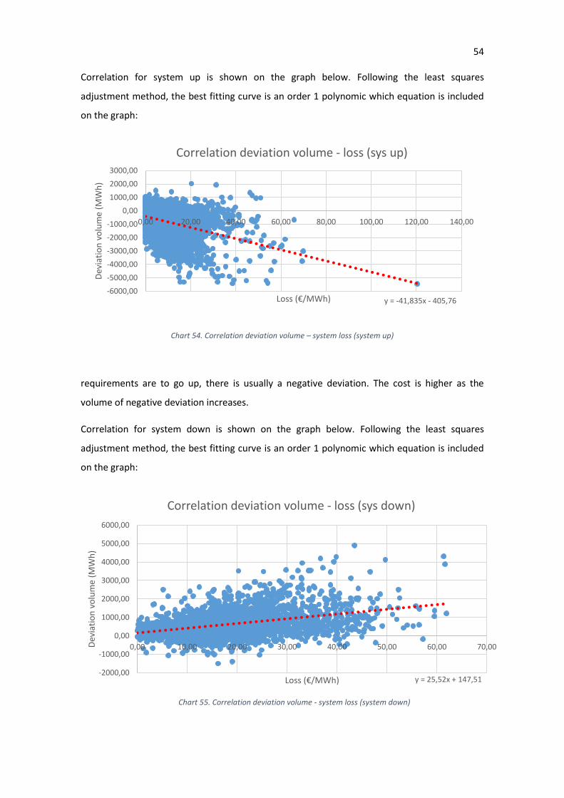
54
Correlation for system up is shown on the graph below. Following the least squares
adjustment method, the best fitting curve is an order 1 polynomic which equation is included
on the graph:
Chart 54. Correlation deviation volume – system loss (system up)
requirements are to go up, there is usually a negative deviation. The cost is higher as the
volume of negative deviation increases.
Correlation for system down is shown on the graph below. Following the least squares
adjustment method, the best fitting curve is an order 1 polynomic which equation is included
on the graph:
y = -41,835x - 405,76-6000,00
-5000,00
-4000,00
-3000,00
-2000,00
-1000,00
0,00
1000,00
2000,00
3000,00
0,00 20,00 40,00 60,00 80,00 100,00 120,00 140,00
Dev
iati
on
vo
lum
e (M
Wh
)
Loss (€/MWh)
Correlation deviation volume - loss (sys up)
y = 25,52x + 147,51-2000,00
-1000,00
0,00
1000,00
2000,00
3000,00
4000,00
5000,00
6000,00
0,00 10,00 20,00 30,00 40,00 50,00 60,00 70,00Dev
iati
on
vo
lum
e (M
Wh
)
Loss (€/MWh)
Correlation deviation volume - loss (sys down)
Chart 55. Correlation deviation volume - system loss (system down)
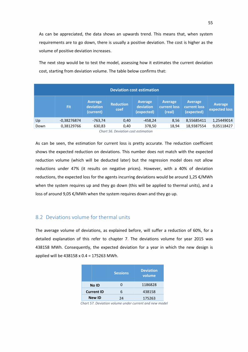
55
As can be appreciated, the data shows an upwards trend. This means that, when system
requirements are to go down, there is usually a positive deviation. The cost is higher as the
volume of positive deviation increases.
The next step would be to test the model, assessing how it estimates the current deviation
cost, starting from deviation volume. The table below confirms that:
As can be seen, the estimation for current loss is pretty accurate. The reduction coefficient
shows the expected reduction on deviations. This number does not match with the expected
reduction volume (which will be deducted later) but the regression model does not allow
reductions under 47% (it results on negative prices). However, with a 40% of deviation
reductions, the expected loss for the agents incurring deviations would be around 1,25 €/MWh
when the system requires up and they go down (this will be applied to thermal units), and a
loss of around 9,05 €/MWh when the system requires down and they go up.
8.2 Deviations volume for thermal units
The average volume of deviations, as explained before, will suffer a reduction of 60%, for a
detailed explanation of this refer to chapter 7. The deviations volume for year 2015 was
438158 MWh. Consequently, the expected deviation for a year in which the new design is
applied will be 438158 x 0.4 = 175263 MWh.
Sessions Deviation volume
No ID 0 1186828
Current ID 6 438158
New ID 24 175263 Chart 57. Deviation volume under current and new model
Deviation cost estimation
Fit Average
deviation (current)
Reduction coef
Average deviation
(expected)
Average current loss
(real)
Average current loss (expected)
Average expected loss
Up -0,38276874 -763,74 0,40 -458,24 8,56 8,55685411 1,25449014
Down 0,38129766 630,83 0,40 378,50 18,94 18,9387554 9,05118427 Chart 56. Deviation cost estimation
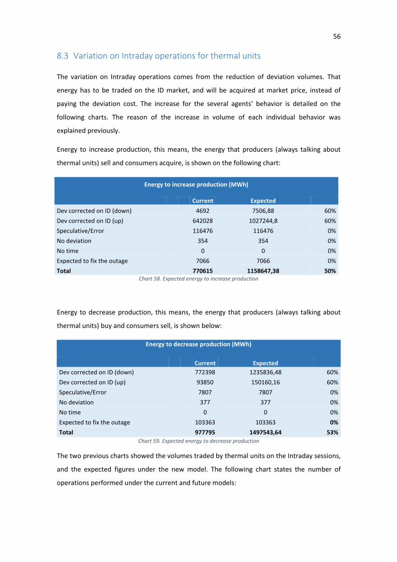
56
8.3 Variation on Intraday operations for thermal units
The variation on Intraday operations comes from the reduction of deviation volumes. That
energy has to be traded on the ID market, and will be acquired at market price, instead of
paying the deviation cost. The increase for the several agents’ behavior is detailed on the
following charts. The reason of the increase in volume of each individual behavior was
explained previously.
Energy to increase production, this means, the energy that producers (always talking about
thermal units) sell and consumers acquire, is shown on the following chart:
Energy to increase production (MWh)
Current Expected
Dev corrected on ID (down) 4692 7506,88 60%
Dev corrected on ID (up) 642028 1027244,8 60%
Speculative/Error 116476 116476 0%
No deviation 354 354 0%
No time 0 0 0%
Expected to fix the outage 7066 7066 0%
Total 770615 1158647,38 50% Chart 58. Expected energy to increase production
Energy to decrease production, this means, the energy that producers (always talking about
thermal units) buy and consumers sell, is shown below:
Energy to decrease production (MWh)
Current Expected
Dev corrected on ID (down) 772398 1235836,48 60%
Dev corrected on ID (up) 93850 150160,16 60%
Speculative/Error 7807 7807 0%
No deviation 377 377 0%
No time 0 0 0%
Expected to fix the outage 103363 103363 0%
Total 977795 1497543,64 53%
Chart 59. Expected energy to decrease production
The two previous charts showed the volumes traded by thermal units on the Intraday sessions,
and the expected figures under the new model. The following chart states the number of
operations performed under the current and future models:
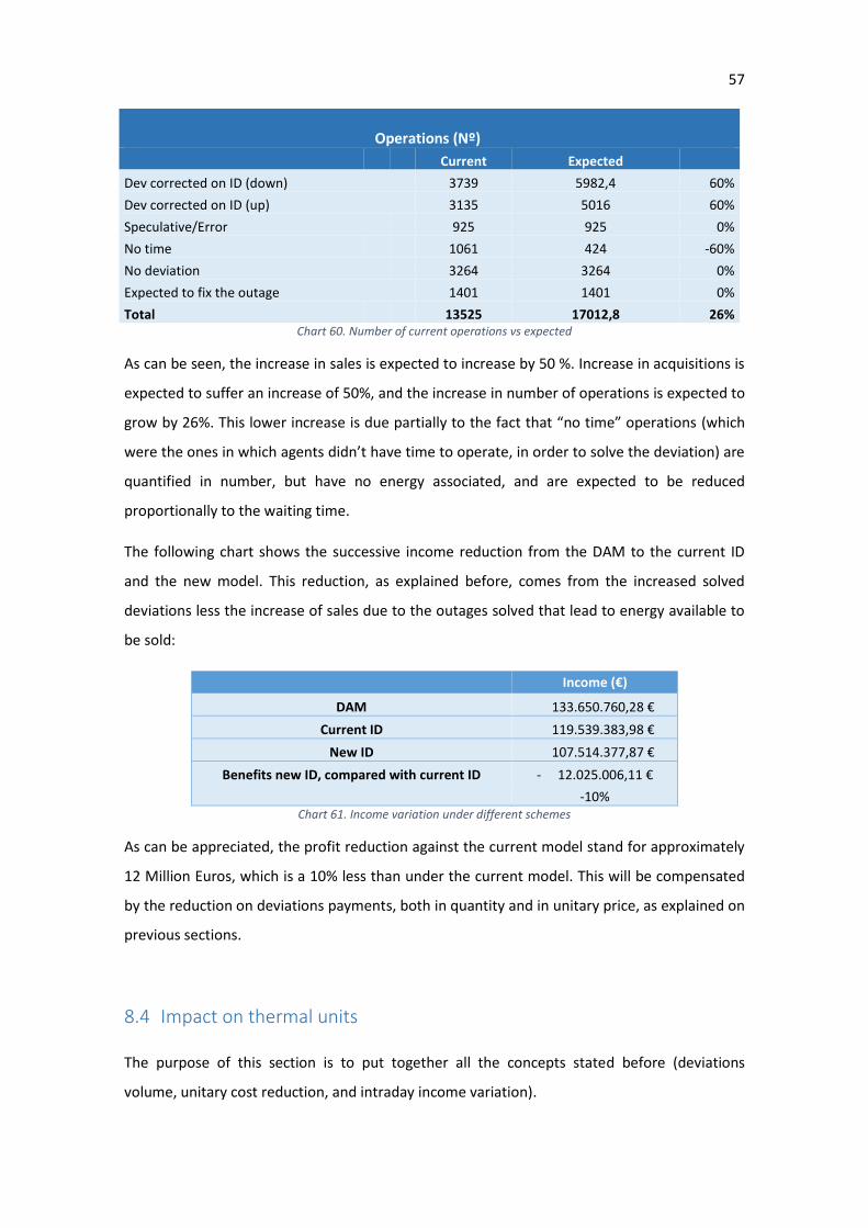
57
Operations (Nº)
Current Expected
Dev corrected on ID (down) 3739 5982,4 60%
Dev corrected on ID (up) 3135 5016 60%
Speculative/Error 925 925 0%
No time 1061 424 -60%
No deviation 3264 3264 0%
Expected to fix the outage 1401 1401 0%
Total 13525 17012,8 26% Chart 60. Number of current operations vs expected
As can be seen, the increase in sales is expected to increase by 50 %. Increase in acquisitions is
expected to suffer an increase of 50%, and the increase in number of operations is expected to
grow by 26%. This lower increase is due partially to the fact that “no time” operations (which
were the ones in which agents didn’t have time to operate, in order to solve the deviation) are
quantified in number, but have no energy associated, and are expected to be reduced
proportionally to the waiting time.
The following chart shows the successive income reduction from the DAM to the current ID
and the new model. This reduction, as explained before, comes from the increased solved
deviations less the increase of sales due to the outages solved that lead to energy available to
be sold:
Income (€)
DAM 133.650.760,28 €
Current ID 119.539.383,98 €
New ID 107.514.377,87 €
Benefits new ID, compared with current ID - 12.025.006,11 €
-10% Chart 61. Income variation under different schemes
As can be appreciated, the profit reduction against the current model stand for approximately
12 Million Euros, which is a 10% less than under the current model. This will be compensated
by the reduction on deviations payments, both in quantity and in unitary price, as explained on
previous sections.
8.4 Impact on thermal units
The purpose of this section is to put together all the concepts stated before (deviations
volume, unitary cost reduction, and intraday income variation).
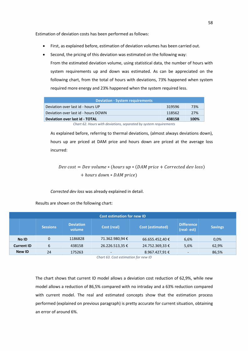
58
Estimation of deviation costs has been performed as follows:
First, as explained before, estimation of deviation volumes has been carried out.
Second, the pricing of this deviation was estimated on the following way:
From the estimated deviation volume, using statistical data, the number of hours with
system requirements up and down was estimated. As can be appreciated on the
following chart, from the total of hours with deviations, 73% happened when system
required more energy and 23% happened when the system required less.
Deviation - System requirements
Deviation over last id - hours UP 319596 73%
Deviation over last id - hours DOWN 118562 27%
Deviation over last id - TOTAL 438158 100% Chart 62. Hours with deviations, separated by system requirements
As explained before, referring to thermal deviations, (almost always deviations down),
hours up are priced at DAM price and hours down are priced at the average loss
incurred:
𝐷𝑒𝑣 𝑐𝑜𝑠𝑡 = 𝐷𝑒𝑣 𝑣𝑜𝑙𝑢𝑚𝑒 ∗ (ℎ𝑜𝑢𝑟𝑠 𝑢𝑝 ∗ (𝐷𝐴𝑀 𝑝𝑟𝑖𝑐𝑒 + 𝐶𝑜𝑟𝑟𝑒𝑐𝑡𝑒𝑑 𝑑𝑒𝑣 𝑙𝑜𝑠𝑠)
+ ℎ𝑜𝑢𝑟𝑠 𝑑𝑜𝑤𝑛 ∗ 𝐷𝐴𝑀 𝑝𝑟𝑖𝑐𝑒)
Corrected dev loss was already explained in detail.
Results are shown on the following chart:
Cost estimation for new ID
Sessions Deviation volume
Cost (real) Cost (estimated) Difference (real- est)
Savings
No ID 0 1186828 71.362.980,94 € 66.655.452,40 € 6,6% 0,0%
Current ID 6 438158 26.226.513,35 € 24.752.369,33 € 5,6% 62,9%
New ID 24 175263 - 8.967.427,91 € - 86,5% Chart 63. Cost estimation for new ID
The chart shows that current ID model allows a deviation cost reduction of 62,9%, while new
model allows a reduction of 86,5% compared with no intraday and a 63% reduction compared
with current model. The real and estimated concepts show that the estimation process
performed (explained on previous paragraph) is pretty accurate for current situation, obtaining
an error of around 6%.
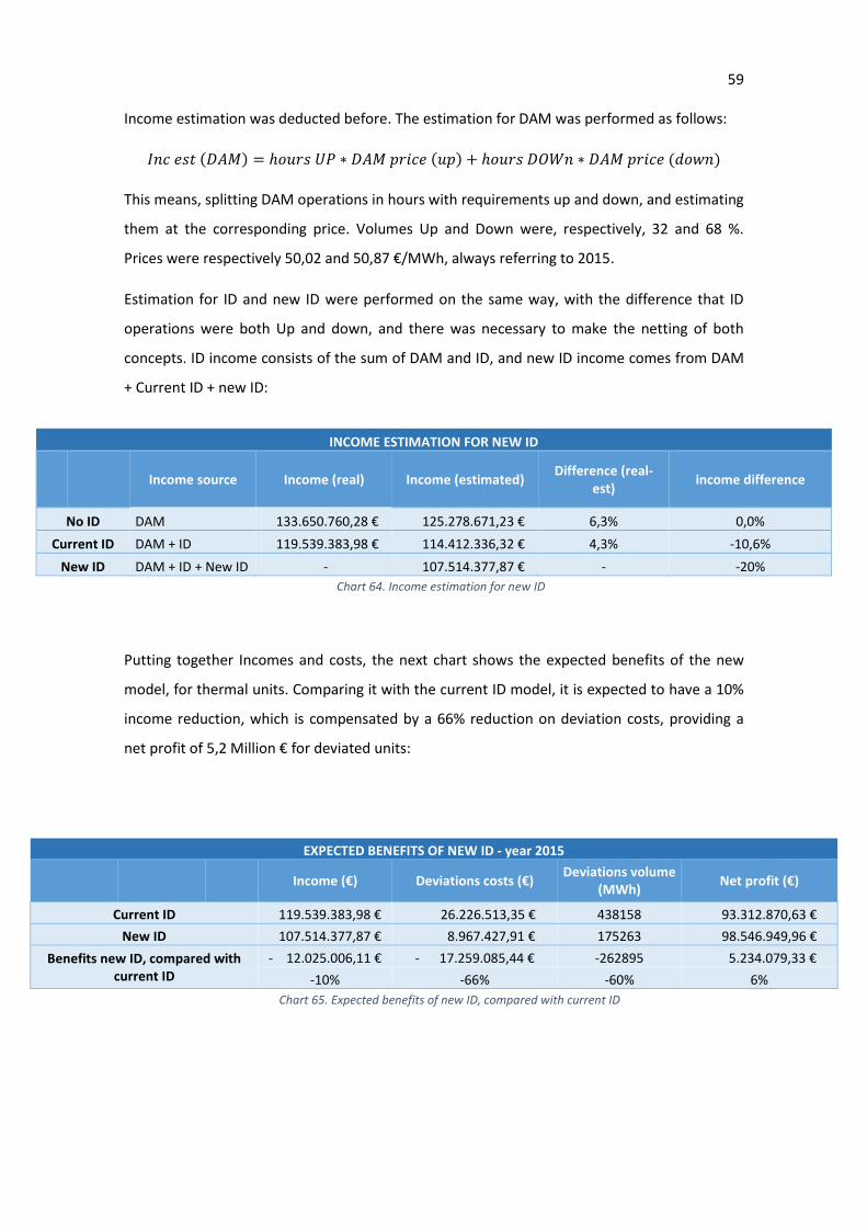
59
Income estimation was deducted before. The estimation for DAM was performed as follows:
𝐼𝑛𝑐 𝑒𝑠𝑡 (𝐷𝐴𝑀) = ℎ𝑜𝑢𝑟𝑠 𝑈𝑃 ∗ 𝐷𝐴𝑀 𝑝𝑟𝑖𝑐𝑒 (𝑢𝑝) + ℎ𝑜𝑢𝑟𝑠 𝐷𝑂𝑊𝑛 ∗ 𝐷𝐴𝑀 𝑝𝑟𝑖𝑐𝑒 (𝑑𝑜𝑤𝑛)
This means, splitting DAM operations in hours with requirements up and down, and estimating
them at the corresponding price. Volumes Up and Down were, respectively, 32 and 68 %.
Prices were respectively 50,02 and 50,87 €/MWh, always referring to 2015.
Estimation for ID and new ID were performed on the same way, with the difference that ID
operations were both Up and down, and there was necessary to make the netting of both
concepts. ID income consists of the sum of DAM and ID, and new ID income comes from DAM
+ Current ID + new ID:
Putting together Incomes and costs, the next chart shows the expected benefits of the new
model, for thermal units. Comparing it with the current ID model, it is expected to have a 10%
income reduction, which is compensated by a 66% reduction on deviation costs, providing a
net profit of 5,2 Million € for deviated units:
Chart 64. Income estimation for new ID
INCOME ESTIMATION FOR NEW ID
Income source Income (real) Income (estimated) Difference (real-
est) income difference
No ID DAM 133.650.760,28 € 125.278.671,23 € 6,3% 0,0%
Current ID DAM + ID 119.539.383,98 € 114.412.336,32 € 4,3% -10,6%
New ID DAM + ID + New ID - 107.514.377,87 € - -20%
Chart 65. Expected benefits of new ID, compared with current ID
EXPECTED BENEFITS OF NEW ID - year 2015
Income (€) Deviations costs (€)
Deviations volume (MWh)
Net profit (€)
Current ID 119.539.383,98 € 26.226.513,35 € 438158 93.312.870,63 €
New ID 107.514.377,87 € 8.967.427,91 € 175263 98.546.949,96 €
Benefits new ID, compared with current ID
- 12.025.006,11 € - 17.259.085,44 € -262895 5.234.079,33 €
-10% -66% -60% 6%
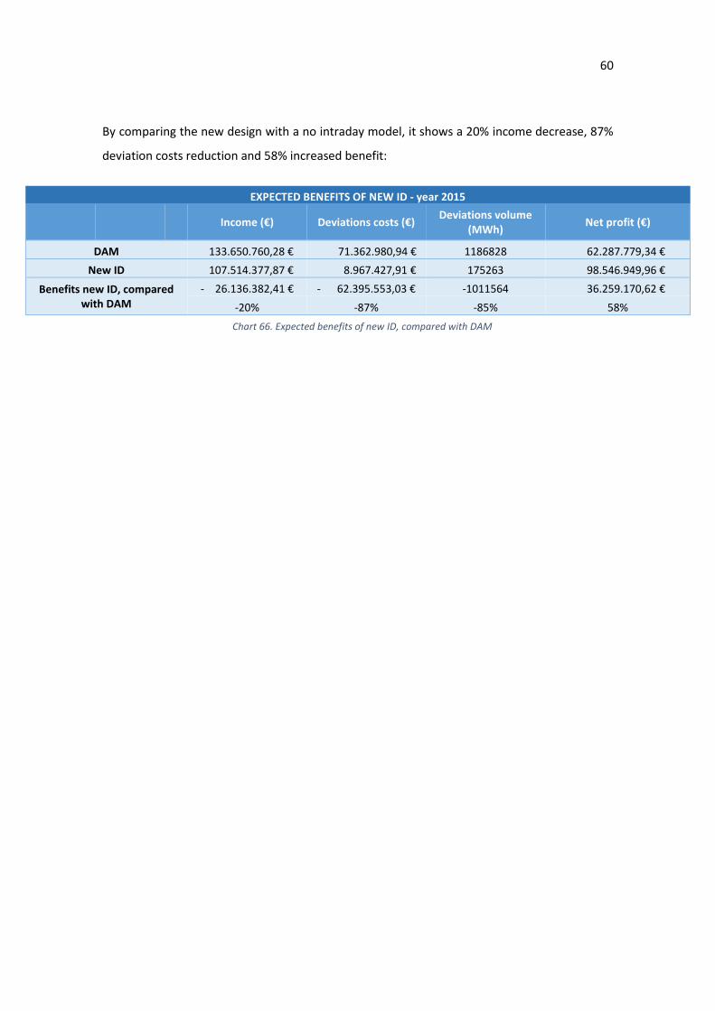
60
By comparing the new design with a no intraday model, it shows a 20% income decrease, 87%
deviation costs reduction and 58% increased benefit:
Chart 66. Expected benefits of new ID, compared with DAM
EXPECTED BENEFITS OF NEW ID - year 2015
Income (€) Deviations costs (€)
Deviations volume (MWh)
Net profit (€)
DAM 133.650.760,28 € 71.362.980,94 € 1186828 62.287.779,34 €
New ID 107.514.377,87 € 8.967.427,91 € 175263 98.546.949,96 €
Benefits new ID, compared with DAM
- 26.136.382,41 € - 62.395.553,03 € -1011564 36.259.170,62 €
-20% -87% -85% 58%

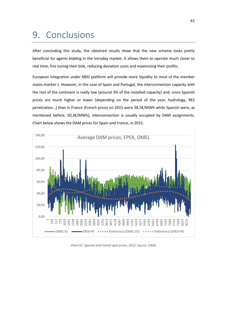
61
9. Conclusions
After concluding this study, the obtained results show that the new scheme looks pretty
beneficial for agents bidding in the Intraday market. It allows them to operate much closer to
real time, fine tuning their bids, reducing deviation costs and maximizing their profits.
European integration under XBID platform will provide more liquidity to most of the member
states market´s. However, in the case of Spain and Portugal, the interconnection capacity with
the rest of the continent is really low (around 3% of the installed capacity) and, since Spanish
prices are much higher or lower (depending on the period of the year, hydrology, RES
penetration…) than in France (French prices on 2015 were 38.5€/MWh while Spanish were, as
mentioned before, 50,3€/MWh), interconnection is usually occupied by DAM assignments.
Chart below shows the DAM prices for Spain and France, in 2015.
Chart 67. Spanish and French spot prices, 2015. Source: OMEL
0,00
20,00
40,00
60,00
80,00
100,00
120,00
140,00
12
59
51
77
75
10
33
12
91
15
49
18
07
20
65
23
23
25
81
28
39
30
97
33
55
36
13
38
71
41
29
43
87
46
45
49
03
51
61
54
19
56
77
59
35
61
93
64
51
67
09
69
67
72
25
74
83
77
41
79
99
82
57
85
15
Average DAM prices, EPEX, OMEL
OMEL ES EPEX-FR Polinómica (OMEL ES) Polinómica (EPEX-FR)
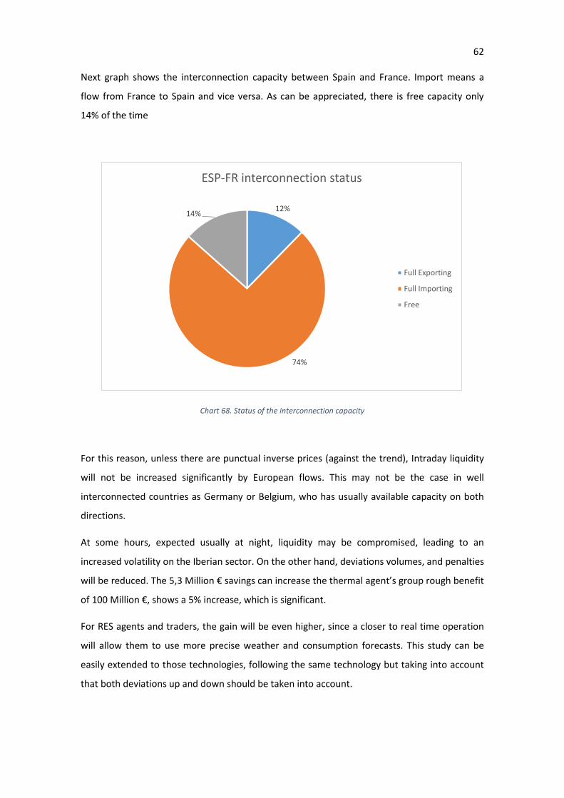
62
Next graph shows the interconnection capacity between Spain and France. Import means a
flow from France to Spain and vice versa. As can be appreciated, there is free capacity only
14% of the time
Chart 68. Status of the interconnection capacity
For this reason, unless there are punctual inverse prices (against the trend), Intraday liquidity
will not be increased significantly by European flows. This may not be the case in well
interconnected countries as Germany or Belgium, who has usually available capacity on both
directions.
At some hours, expected usually at night, liquidity may be compromised, leading to an
increased volatility on the Iberian sector. On the other hand, deviations volumes, and penalties
will be reduced. The 5,3 Million € savings can increase the thermal agent’s group rough benefit
of 100 Million €, shows a 5% increase, which is significant.
For RES agents and traders, the gain will be even higher, since a closer to real time operation
will allow them to use more precise weather and consumption forecasts. This study can be
easily extended to those technologies, following the same technology but taking into account
that both deviations up and down should be taken into account.
12%
74%
14%
ESP-FR interconnection status
Full Exporting
Full Importing
Free

63
However, this study is based on reasoned estimations. The results obtained are estimative and
subject to an error.


64
10. Bibliography
XBID Project (APX/Belpex, EPEX SPOT, NordPool Spot, OMIE and GME)
http://www.omie.es/files/160126%203rd%20UG%20presentation_final.pdf
http://www.omie.es/files/150428%20XBID_2.%20User_Group_Meeting_Slides
_final.pdf
http://www.omie.es/files/141125_user_group_meeting_final.pdf
REE Operative Procedures:
P.O. 3.3 – Deviations Management
P.O. 7.2 – Secondary Regulation
P.O. 7.3 – Tertiary Regulation
P.O. 14.4 – Payment rights/obligations derived from balancing services
OMIE Market Rules
http://www.omie.es/files/reglas_mercado_0.pdf
REE Adjustment Services Report
http://www.ree.es/sites/default/files/downloadable/ajuste_informe_sistema_
electrico_2015.pdf


![Master`s Degree Program: KINESIOLOGY Education ... [2sem].pdf · Master`s Degree Program: KINESIOLOGY Education-qualification degree: MASTER Proffessional qualification: Kinesiologist](https://img.dokumen.tips/doc/110x75/5abf482e7f8b9a5d718e133a/masters-degree-program-kinesiology-education-2sempdfmasters-degree-program.jpg)