Odour Assessment – Narrandera Poultry Project – Farm 1 F... · report odour assessment – narrandera poultry project – farm 1 proten holdings pty limited job id. 08976 5 september

A

PP

EN

DIX

F

Report

ODOUR ASSESSMENT – NARRANDERA POULTRY PROJECT – FARM 1

PROTEN HOLDINGS PTY LIMITED

Job ID. 08976

5 September 2014

8976 Proten Narrandera Poultry Project R1-1.docx ii

Job ID 08976 | QLD-AQ-002-08976

PROJECT NAME: Odour Assessment – Narrandera Poultry Project – Farm

1

JOB ID: 08976

DOCUMENT CONTROL NUMBER QLD-AQ-002-08976

PREPARED FOR: ProTen Holdings Pty Limited

APPROVED FOR RELEASE BY: R. Ormerod

DISCLAIMER & COPYRIGHT: This report is subject to the copyright statement

located at www.pacific-environment.com © Pacific

Environment Operations Pty Ltd ABN 86 127 101 642

DOCUMENT CONTROL

VERSION DATE PREPARED BY REVIEWED BY

D1-1 04.09.14 M.Wilson G.Galvin

R1-1 05.09.14 G.Galvin R. Ormerod

Pacific Environment Operations Pty Ltd: ABN 86 127 101 642

BRISBANE

Level 1, 59 Melbourne Street, South Brisbane Qld 4101

PO Box 3306, South Brisbane Qld 4101

Ph: +61 7 3004 6400

Fax: +61 7 3844 5858

Unit 1, 22 Varley Street

Yeerongpilly, Qld 4105

Ph: +61 7 3004 6460

ADELAIDE

35 Edward Street, Norwood SA 5067

PO Box 3187, Norwood SA 5067

Ph: +61 8 8332 0960

Fax: +61 7 3844 5858

SYDNEY Suite 1, Level 1, 146 Arthur Street

North Sydney, NSW 2060

Ph: +61 2 9870 0900

Fax: +61 2 9870 0999

MELBOURNE

Level 10, 224 Queen Street

Melbourne Vic 3000

Ph: +61 3 9036 2637

Fax: +61 2 9870 0999

PERTH

Level 1, Suite 3

34 Queen Street, Perth WA 6000

Ph: +61 8 9481 4961

Fax: +61 2 9870 0999

http://www.pacific-environment.com/

8976 Proten Narrandera Poultry Project R1-1.docx iii

Job ID 08976 | QLD-AQ-002-08976

DISCLAIMER

Pacific Environment acts in all professional matters as a faithful advisor to the Client and exercises all

reasonable skill and care in the provision of its professional services.

Reports are commissioned by and prepared for the exclusive use of the Client. They are subject to and

issued in accordance with the agreement between the Client and Pacific Environment. Pacific

Environment is not responsible for any liability and accepts no responsibility whatsoever arising from the

misapplication or misinterpretation by third parties of the contents of its reports.

Except where expressly stated, Pacific Environment does not attempt to verify the accuracy, validity or

comprehensiveness of any information supplied to Pacific Environment for its reports.

Reports cannot be copied or reproduced in whole or part for any purpose without the prior written

agreement of Pacific Environment.

Where site inspections, testing or fieldwork have taken place, the report is based on the information

made available by the client or their nominees during the visit, visual observations and any subsequent

discussions with regulatory authorities. The validity and comprehensiveness of supplied information has

not been independently verified and, for the purposes of this report, it is assumed that the information

provided to Pacific Environment is both complete and accurate. It is further assumed that normal

activities were being undertaken at the site on the day of the site visit(s), unless explicitly stated

otherwise.

8976 Proten Narrandera Poultry Project R1-1.docx iv

Job ID 08976 | QLD-AQ-002-08976

CONTENTS

1 INTRODUCTION 6 1.1 Background 6 1.2 Study Objectives 6 1.3 Study Approach 7

2 EMISSION ESTIMATION 8 2.1 Odour Emission Estimation 8

2.1.1 Basis of Odour Emissions Data 8 2.1.2 Analysis of Odour Data 8 2.1.3 Odour Emissions Estimation 9 2.1.4 Particulate Emissions 13

3 METEOROLOGICAL MODELLING 18 3.1 TAPM 18 3.2 CALMET 18

4 EXISTING ENVIRONMENT 19 4.1 Site Meteorology 19

4.1.1 Wind 19 4.1.2 Stability 22 4.1.3 Mixing Height 23

4.2 Existing Air Quality 24

5 DISPERSION MODELLING 26 5.1 CALPUFF 26 5.2 CALPUFF Setup 26

6 IMPACT ASSESSMENT CRITERIA 29 6.1 Particulate Matter 29 6.2 Odour 29

6.2.1 Measuring odour concentration 29 6.2.2 Odour performance criteria 29

7 RESULTS 32 7.1 Odour Impacts 32 7.2 Particulate Matter 33 7.3 Cumulative Assessment 36

7.3.1 Odour 36 7.3.2 Annual average PM10 36 7.3.3 24 hour average PM10 36

8 CONCLUSION 38

9 RECOMMENDATIONS 39

10 REFERENCES 40

8976 Proten Narrandera Poultry Project R1-1.docx v

Job ID 08976 | QLD-AQ-002-08976

LIST OF FIGURES

Figure 1-1: Subject Site and Proposed Sheds 6

Figure 1-2: Assessment methodology 7

Figure 2-1: Data used in odour emissions modelling 9

Figure 2-2: Average bird weight by age 10

Figure 2-3: Example of modelled shed OER variations over time for the proposed sheds (K=2.2) 12

Figure 2-4: Modelled Shed OER Variations Over Time for the Project (k=2.2) 13

Figure 2-5: Mirrabooka Data 14

Figure 2-6: Relationship Between Particulate Concentration and Flow Rate 14

Figure 2-7: Summary of Measured PM10 data (PE), CRC Data and Pacific Environment emissions model

data for a typical farm 16

Figure 2-8: Comparison of CRC Data and revised Pacific Environment emissions model data for a

typical farm 17

Figure 2-9: Example of Modelled Shed PM10 Variations Over Time for a Grow Out Cycle 17

Figure 4-1: Wind rose for the proposed site 20

Figure 4-2: Time of day wind roses for the proposed site 21

Figure 4-3: Wind Speed Frequency (hourly average) for 2010 22

Figure 4-4: Frequency Distribution of Estimated Pasquill- Gifford Stability Classes for 2010 23

Figure 4-5: Estimated Mixing Height versus Hour of Day for 2010 24

Figure 5-1: Shed point source locations 27

Figure 5-2: Receptor locations 28

Figure 7-1: Predicted 1-second peak-to-mean concentration 33

Figure 7-2: Predicted maximum 24-hour PM10 concentration 35

Figure 7-3: Predicted annual average PM10 concentration 36

Figure 7-4: Predicted Number of Days Over 24-Hour average PM10 Concentration 37

LIST OF TABLES

Table 2-1: Example - Shed ventilation as a percentage of maximum ventilation 11

Table 4-1: Description of Atmospheric Stability Class 23

Table 4-2: PM10 TEOM data from the EPA Albury monitoring station 25

Table 6-1: Air Quality Impact Assessment Criteria for Particulate Matter Concentrations 29

Table 6-2: Odour Performance Criteria for the Assessment of Odour 30

Table 6-3: Factors for estimating peak concentrations on flat terrain 31

Table 7-1: Predicted odour concentrations at the nearest receptors 32

Table 7-2: Predicted PM10 concentrations at the nearest receptors 34

8976 Proten Narrandera Poultry Project R1-1.docx 6

Job Number 08976 | QLD-AQ-002-08976

1 INTRODUCTION

Pacific Environment Limited was engaged by SLR Consulting Australia Pty. Ltd. (SLR) on behalf of ProTen

Holdings Pty Limited (ProTen) to prepare an odour and dust assessment of a proposed intensive poultry

broiler production complex (“Narrandera Poultry Production Complex Farm 1”) located near

Narrandera in south-western New South Wales (NSW).

1.1 Background

The proposed poultry development site will comprise two poultry production units (PPU). Each PPU will

consist of 16 tunnel-ventilated, fully-enclosed and climate-controlled poultry sheds. Each shed will have

the capacity to house a maximum of 49,000 birds (at 18 birds per square metre). As a result each PPU

will have a population of up to 784,000 birds and a potential total farm population of 1,568,000 birds.

The subject site is shown in Figure 1-1. The PPU on the west in the figure has fans facing to the west, and

the eastern PPU has fans facing to the east.

Figure 1-1: Subject Site and Proposed Sheds

1.2 Study Objectives

The objective of this assessment is to determine odour and dust impacts from the operation in

accordance with relevant methods. The study has been performed in accordance with the

Environment Protection Authority’s (EPA) “Approved methods for the modelling and assessment of air

pollutants in NSW” (NSW EPA, 2005) (herein referred to as the Approved Methods) and the EPA

document “Assessment and management of odours from stationary sources in NSW” (NSW EPA, 2006).



1.3 Study Approach

The methodology for this project included the following stages (see Figure 1-2):

information and data review

emissions estimation

meteorological data processing

plume dispersion modelling.

assessment of impacts on surroundings

reporting.

Figure 1-2: Assessment methodology



2 EMISSION ESTIMATION

2.1 Odour Emission Estimation

The odour emissions model of Ormerod and Holmes (2005) was used for this assessment. The

methodology is commonly used in Australia and New Zealand and is consistent with that

recommended in the Best Practice Guidance for the Queensland Poultry Industry - Plume Dispersion

Modelling and Meteorological Processing (PAEHolmes, 2011) as prepared for the Queensland

Government for inclusion in the Queensland Guidelines Meat Chicken Farms (DAFF, 2012).

2.1.1 Basis of Odour Emissions Data

Odour emission rates (OERs) for this assessment were based on data from a variety of meat chicken

farms in Australia, as well as theoretical considerations.

The approach generates hourly varying emission rates from meat chicken farm sheds based on the

following factors:

the number of birds, which varies later in the batch as harvesting takes place

the stocking density of birds, which is a function of bird numbers, bird age and shed size

ventilation rate, which depends on bird age and ambient temperature

design and management practices, particularly those aimed at controlling litter moisture.

Data from existing farms were gathered from tunnel-ventilated sheds (many with nipple drinkers) and

chicken batches at approximately five weeks of age or more. Given that maximum emissions occur

around 5 weeks and later, these samples represent the maximum odour generating potential.

2.1.2 Analysis of Odour Data

Odour data from various farms and under various conditions were standardised to relate the OER per

unit bird density and shed area to the ventilation rate at the time of sampling. The resulting relationship

is shown in Figure 2-1. The data can be segregated into two groups:

farms operating under typical conditions

farms that were experiencing elevated odour emissions due to problems with shed design or

management at the time of sampling.

High moisture litter is a common issue that can lead to increased odour emissions (Clarkson &

Misselbrook, 1991). High moisture litter can be caused by using foggers in heatwave conditions, which

was once common with older shed designs, and water spillage from drinkers, which can be avoided

with newer technology. More frequent changing of litter between batches also minimises odour

impacts. A vigilant approach to identifying and removing wet litter is now a well-accepted tenet of

management.

Design factors include inadequate ventilation and retrofitted sheds. Many older sheds had lower

maximum ventilation rates than newer sheds, thereby reducing the effectiveness of airflow to control

litter moisture. Retrofitted sheds also did not often have the insulation properties of new sheds and were

therefore more difficult to cool by ventilation in hot weather.

As illustrated by Figure 2-1, the degree to which these issues affect odour levels is highly variable. The

curves represent a conservative estimate of the relationship between ambient temperature and odour

emissions for tunnel ventilated sheds operating under varying degrees of management. The ’best’

curve (green) represents a well-designed and managed shed with a high level of control over (for

example) litter moisture levels. The ’worst’ curve (red) represents a shed experiencing difficulties due to

factors such as adverse weather conditions, equipment failure, poor design or management, or a

combination of these factors.



Most of the farms for which data are presented in Figure 2-1 differ significantly from the best practice

design and management criteria for modern farms which include:

efficient mechanical ventilation

nipple and cup drinkers

fully insulated sheds

impervious floors

single or dual batch litter usea

daily litter inspection and replacement (if litter becomes wet).

Figure 2-1: Data used in odour emissions modelling

2.1.3 Odour Emissions Estimation

From Figure 2-1, the relationship between the ’standardised’ OER and shed ventilation is expressed as:

OERS = 0.025 K V 0.5 (1)

where:

OERS = standardised odour emission rate (ou.m³/s) per unit shed area (m²) per unit of bird density (in

kg/m²)

V = ventilation rate (m³/s)

K = scaling factor between 1 and 5b where a value of 1 represents a very well designed and managed

shed operating with minimal odour emissions.

a The most recent research has shown no significant difference between single and dual use litter see Poultry CRC. b Note that a K factor of 4-5 would be very uncommon and would represent a shed with serious odour

management issues.



The scaling factor (K) referred to in equations 1 and 2 is essentially a scale rating for the design and

management of the sheds. The calculation of K for any given farm is based on several components of

farm management. For new farms conforming to best practice it is recommended that the value of K

be set at 2.2 (PAEHolmes, 2011).

Analysis of data for other Proten Farms (held by PE) has shown that the average K factor over time

typically is at or below K = 2.

Equation 1 can be expanded to provide a prediction of the OER from a shed at any given stage of the

growth cycle as follows:

OER = 0.025 K A D V 0.5 (2)

where:

OER = odour emission rate (ou.m³/s)

A = total shed floor area (m²)

D = average bird density (in kg/m²)

Bird density (D) is related to the age of the birds and the stocking density (i.e. the number of birds

placed per unit area). It is common practice within the meat chicken industry to vary the stocking

density with the time of year and market demands. Lower ambient temperatures during the winter

months allow for higher bird densities. For this assessment, based on proposed operations, a maximum

stocking density of 18 birds/m2 has been used. With a known stocking density, a value of the mass per

unit area can be estimated based on the relationship shown in Figure 2-2.

Figure 2-2: Average bird weight by agec

The ventilation rate (V) at any given time is a function of the age of the birds and the ambient

temperature and humidity. Table 2-1 provides an estimate of the ventilation required for a tunnel

ventilated shed as a percentage of the maximum for summertime conditions.

c Source: Ross Broiler Manual www.ross-intl.aviagen.com.

0

500

1000

1500

2000

2500

3000

3500

4000

4500

0 10 20 30 40 50 60 70

day of cycle

avera

ge b

ird

weig

ht

(g)



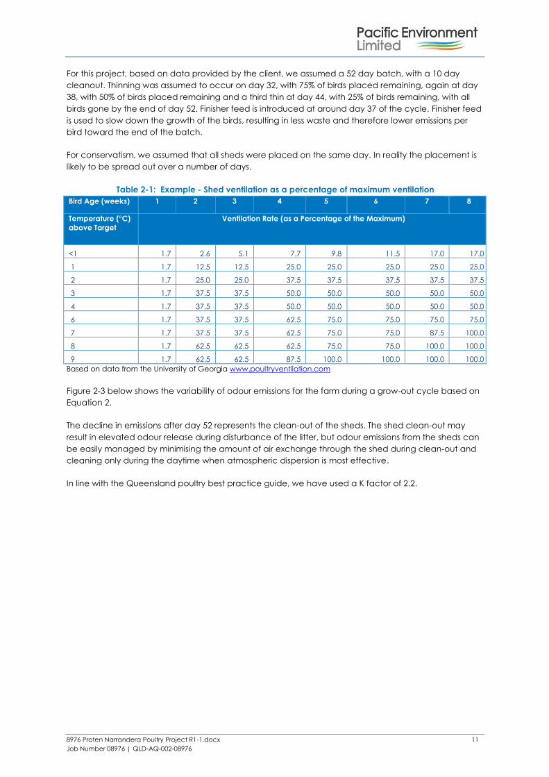
For this project, based on data provided by the client, we assumed a 52 day batch, with a 10 day

cleanout. Thinning was assumed to occur on day 32, with 75% of birds placed remaining, again at day

38, with 50% of birds placed remaining and a third thin at day 44, with 25% of birds remaining, with all

birds gone by the end of day 52. Finisher feed is introduced at around day 37 of the cycle. Finisher feed

is used to slow down the growth of the birds, resulting in less waste and therefore lower emissions per

bird toward the end of the batch.

For conservatism, we assumed that all sheds were placed on the same day. In reality the placement is

likely to be spread out over a number of days.

Table 2-1: Example - Shed ventilation as a percentage of maximum ventilation

Bird Age (weeks) 1 2 3 4 5 6 7 8

Temperature (°C)

above Target

Ventilation Rate (as a Percentage of the Maximum)

<1 1.7 2.6 5.1 7.7 9.8 11.5 17.0 17.0

1 1.7 12.5 12.5 25.0 25.0 25.0 25.0 25.0

2 1.7 25.0 25.0 37.5 37.5 37.5 37.5 37.5

3 1.7 37.5 37.5 50.0 50.0 50.0 50.0 50.0

4 1.7 37.5 37.5 50.0 50.0 50.0 50.0 50.0

6 1.7 37.5 37.5 62.5 75.0 75.0 75.0 75.0

7 1.7 37.5 37.5 62.5 75.0 75.0 87.5 100.0

8 1.7 62.5 62.5 62.5 75.0 75.0 100.0 100.0

9 1.7 62.5 62.5 87.5 100.0 100.0 100.0 100.0

Based on data from the University of Georgia www.poultryventilation.com

Figure 2-3 below shows the variability of odour emissions for the farm during a grow-out cycle based on

Equation 2.

The decline in emissions after day 52 represents the clean-out of the sheds. The shed clean-out may

result in elevated odour release during disturbance of the litter, but odour emissions from the sheds can

be easily managed by minimising the amount of air exchange through the shed during clean-out and

cleaning only during the daytime when atmospheric dispersion is most effective.

In line with the Queensland poultry best practice guide, we have used a K factor of 2.2.

http://www.poultryventilation.com/



Figure 2-3: Example of modelled shed OER variations over time for the proposed sheds (K=2.2)

Figure 2-4 below shows the variability of estimated odour emissions for the Project for a year of

operations as the emissions vary based on Equation 2. The drop in overall emissions midway through the

year corresponds to lower temperatures in the late autumn and winter months which result in lower

ventilation rates and therefore less odour emissions from the PPUs.



Figure 2-4: Modelled Shed OER Variations Over Time for the Project (k=2.2)

2.1.4 Particulate Emissions

We estimated particulate emission rates for this study using a modelling approach based on data from

meat chicken farms in NSW and Queensland as well as theoretical considerations.

The approach generates hourly varying emission rates from each shed based on the following factors:

the total weight of all of birds, which varies later in the batch as harvesting takes place

ventilation rate, which depends on bird age and ambient temperature

design and management practices.

First we examined data from an existing farm in NSW with tunnel-ventilated sheds and cup drinkers.

Data were gathered a limited number of times for chicken batches between one to eight weeks of

age. These samples represent particulate emissions over a full batch cycle.

The data detailed in Mirrabooka (2002) were standardised to relate the particulate matter

concentration to the total bird mass at the time of sampling. The resulting relationship is shown in Figure

2-5. The shed ventilation rate was also related to particulate matter concentration (as a fraction of the

maximum) and is presented in Figure 2-6.

The data were gathered between July and August and therefore may not represent all meteorological

conditions. When collected, Mirrabooka (2002) showed that the emission factors generated from these

data were comparable to Victorian EPA recommended emission rates. However since 2002 significant

improvements have been made in poultry production.



Figure 2-5: Mirrabooka Data

Figure 2-6: Relationship Between Particulate Concentration and Flow Rate

Using Figure 2-5(Mirrabooka data) a relationship between the maximum particulate emission

concentration (PEC) and bird mass, assuming a single fan operating, is expressed as:

baMPEC (3)

where:

PEC = maximum particulate emission concentration (mg/m³)

M = Total mass of birds (tonnes)

a = 0.270 for TSP or 0.115 for PM10

0.0

2.0

4.0

6.0

8.0

10.0

12.0

14.0

16.0

18.0

0 5 10 15 20 25 30 35 40 45 50

Total Bird Mass (tonnes)

Co

ncen

trati

on

(m

g/N

m3)

PM10 TSP

0.0

0.2

0.4

0.6

0.8

1.0

1.2

0 10 20 30 40 50 60 70 80 90

Flow Rate (m³/s)

Fra

cti

on

of

Maxim

um

Co

ncen

trati

on

TSP PM10



b = 0.385 for TSP or 0.917 for PM10

To account for the dilution that occurs under higher flow rates, equation (4) has been taken from Figure

2-6:

)(* d

v cVPECPEC (4)

where:

PECv = particulate emission concentration (mg/m³)


V = Ventilation rate (m³/s) and

c = 3.3 for TSP and 4.11 for PM10

d = -0.49 for TSP and –0.58 for PM10

A particulate matter emission rate (PER) can be calculated by multiplying the PEC by the ventilation

rate (V).

The ventilation rate (V) used at any given time is a function of the age of the birds and the ambient

temperature and humidity.

More recently two new datasets became available. The first was the PM10 emission data detailed in

Australian Poultry CRC (2011) and the second was data collected by Pacific Environment at a farm in

South East Queensland (PAEHolmes, 2012). These data are compared in Figure 2-7 as standardised for

number of birds and bird age. As there is a relatively consistent relationship between bird age bird mass

(across the industry) the data in Figure 2-7 are comparable from site to site. The data are presented as

follows:

Green Markers – Emissions predicted based on the data in

Red markers – Data from PAEHolmes (2012)d

Blue Markers – CRC data from Australian Poultry CRC (2011)

From the data, it can be seen that emission rates predicted using the method based on the

Mirrabooka data are much higher than those from the latest data.

d These data were collected over a period of five days every 15 minutes during summer just after first thinout. Due to

project limitations ventilation rates were unable to be measured in real time. The data shown in the figure therefore

represents the range of potential concentrations over a range of ventilation rates. The data showed a typical trend

of low concentrations overnight, corresponding with conditions where lower ventilation rates are required. During

the day the concentrations typically were consistent over the day when elevated ventilation levels were required

(as the ambient temperature was above target temperature) with some peaks from time to time corresponding with

short term ventilation changes.



Figure 2-7: Summary of Measured PM10 data (PE), CRC Data and Pacific Environment

emissions model data for a typical farm

Based on the more recent data (which is representative of current shed management) in Figure 2-7 a

revised emission equation was developed (5)

459.0058.0 MPEC (5)

where:


M = Total mass of birds (tonnes)

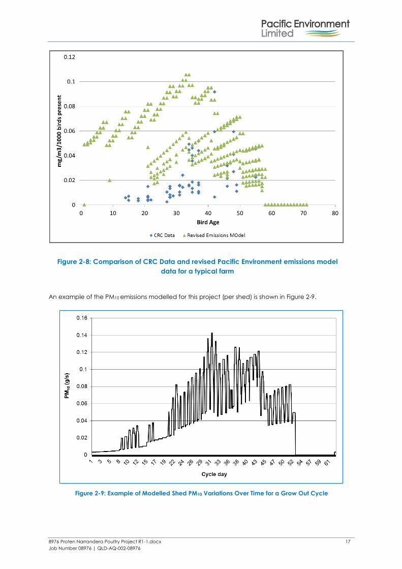
An example of the new relationship is shown in Figure 2-8. As shown in the figure, the emissions

estimation method remains conservative in that it still estimates in shed concentrations above the

maximum CRC data values.



Figure 2-8: Comparison of CRC Data and revised Pacific Environment emissions model

data for a typical farm

An example of the PM10 emissions modelled for this project (per shed) is shown in Figure 2-9.

Figure 2-9: Example of Modelled Shed PM10 Variations Over Time for a Grow Out Cycle



3 METEOROLOGICAL MODELLING

The climate and meteorology of a site are fundamentally important to the dispersion of atmospheric

emissions. A good quality meteorological dataset is therefore necessary to model the dispersion of air

emissions. A representative meteorological year of 2010 was selected for use in this project based on

long-term averagese.

The meteorological data used in the dispersion modelling was processed in two steps. Synoptic scale

meteorological data were first processed in The Air Pollution Model (TAPM) and then further processed

in CALMET to produce the wind field and weather data suitable for dispersion modelling with CALPUFF.

This method is known as the No Observation approach as detailed in the Generic Guidance and

Optimum Model Settings for the CALPUFF modelling system for inclusion into the 'Approved methods for

the Modeling and Assessment of Air Pollutants in NSW (NSW OEH, 2011). The no observation approach is

considered appropriate for regulatory screening modelling.

Prior to performing the modelling we examined hourly BOM data for the area. Based on our analysis we

concluded that 2010 was representative of long term trends for the area (in particular wind speeds).

Hence 2010 was the year modelled for the project.

3.1 TAPM

TAPM (version 4), is a three dimensional meteorological and air pollution model developed by the

CSIRO Division of Atmospheric Research. Detailed description of the TAPM model is provided in the

TAPM user manual (Hurley P, 2008a). The Technical Paper on TAPM (Hurley P, 2008b) describes technical

details of the model equations, parameterisations, and numerical methods. A summary of some

verification studies using TAPM is also available (Hurley P, 2008c).

TAPM v4 solves the fundamental fluid dynamics and scalar transport equations to predict meteorology

and (optionally) pollutant concentrations. It consists of coupled prognostic meteorological and air

pollution concentration components. The model predicts airflow important to local scale air pollution,

such as sea breezes and terrain induced flows, against a background of larger scale meteorology

provided by synoptic analyses.

The output data from TAPM was input into CALMET.

3.2 CALMET

CALMET is the meteorological pre-processor to CALPUFF and includes a wind field generator containing

objective analysis and parameterised treatments of slope flows, terrain effects, and terrain blocking

effects. The pre-processor uses the meteorological inputs in combination with land use and geophysical

information for the modelling domain to predict a gridded three dimensional meteorological field

(containing data on wind components, air temperature, relative humidity, mixing height, and other

micro meteorological variables) for the domain used in the CALPUFF dispersion model.

CALMET uses the meteorological data input in combination with land use and geophysical information

to predict a gridded meteorological field for the modelling domain. The gridded TAPM generated data

were processed in CALMET with fine terrain resolution (100 m grid point spacing) for an inner domain of

approximately 12 km x 8 km domain.

e Further details on meteorological year selection can be provided upon request.



4 EXISTING ENVIRONMENT

4.1 Site Meteorology

The primary meteorological parameters involved in modelling plume dispersion from poultry sheds are

wind direction, wind speed, turbulence (atmospheric stability) and mixing height (depth of turbulent

layer). The meteorological data for 2010 as generated by CALMET and used in the dispersion modelling

are discussed below.

4.1.1 Wind

The wind roses show the frequency of occurrence of winds by direction and strength. The bars

correspond to the 16 compass points (north, north-north-east, north-east etc). The bar at the top of

each wind rose diagram represents winds blowing from the north (i.e. northerly winds), and so on. The

length of the bar represents the frequency of occurrence of winds from that direction, and the colour

and width of the bar sections correspond to wind speed categories, as per the legend. Thus it is

possible to visualise how often winds of a certain direction and strength occur over any period of time.

The wind roses plotted from data extracted from CALMET is presented in Figure 4-1 and Figure 4-2. The

annual wind rose (Figure 4-1) shows that the most common wind directions are southwest and

northeast. In the early morning and late at night, winds are typically light (<3 m/s) and from the

southwest or northeast depending on the time of year. During the morning (7am to 12 noon) the winds

are typically stronger than overnight and from a variety of directions, but with a low frequency from the

southeast. During the early afternoon the winds are also from these directions, but are on occasion

stronger and with a higher frequency of winds from the south west.

Overall the wind data show a high frequency of calm to light winds (up to 3 m/s), occurring 48% of the

time.



Location:

Proposed Narrandera Poultry

Production Complex

Data Period:

2010

Data Type:

CALMET extract

Calm winds:

0.01%

Average wind speed:

3.1 m/s

Plot:

M.Wilson

Figure 4-1: Wind rose for the proposed site



12 AM to 6 AM

7 AM to 12 PM

1 PM to 6 PM

7 PM to 12 AM

Time of day Average wind speed

(m/s)

Calm winds frequency %

12 AM to 6 AM 2.6 0.0

7 AM to 12 PM 3.7 0.1

1 PM to 6 PM 3.6 0.0

7 PM to 12 AM 2.5 0.0

Location:

Proposed Narrandera

Poultry Production

Complex

Data Period:

2010

Data Type:

CALMET extract

Plot:

M.Wilson

Figure 4-2: Time of day wind roses for the proposed site

The wind speed frequency is shown in Figure 4-3.



Figure 4-3: Wind Speed Frequency (hourly average) for 2010

4.1.2 Stability

Atmospheric turbulence is an important factor in air dispersion. Turbulence acts to increase the cross-

sectional area of the plume due to random motions, thus diluting or diffusing a plume. As turbulence

increases, the rate of plume dilution or diffusion increases. Turbulence is related to the vertical

temperature gradient, which determines what is known as stability, or thermal stability. For traditional

dispersion modelling using Gaussian plume models, categories of atmospheric stability are used in

conjunction with other meteorological data to describe atmospheric conditions and thus dispersion.

The most well-known stability classification is the Pasquill-Gifford scheme, which denotes stability classes

from A to F. Class A is described as highly unstable and occurs in association with strong surface

heating and light winds, leading to intense convective turbulence and much enhanced plume dilution.

At the other extreme, class F denotes very stable conditions associated with strong temperature

inversions and light winds, which commonly occur under clear skies at night and in the early morning.

Under these conditions plumes can remain relatively undiluted for considerable distances downwind.

Intermediate stability classes grade from moderately unstable (B), through neutral (D) to slightly stable

(E). Whilst classes A and F are strongly associated with clear skies, class D is linked to windy and/or

cloudy weather, and short periods around sunset and sunrise when surface heating or cooling is small.

Pasquil-Gifford stability classes indicate the characteristics of the prevailing meteorological conditions

and are estimated based on a number of meteorological parameters. Pasquil-Gifford stability classes

are not specifically used as input data for the CALPUFF dispersion modelling, and are used here to help

describe conditions at the site. A summary of atmospheric stability classes is provided in Table 4-1.

0.0%0.6%

2.5%

10.0%

20.7%

14.5%

9.9%

15.1%

19.7%

6.1%

0.9%

0.0%

0%

2%

4%

6%

8%

10%

12%

14%

16%

18%

20%

22%

0 0.5 1 1.5 2 2.5 3 4 6 8 10 >10

Fre

qu

en

cy

Wind Speed (m/s)



Table 4-1: Description of Atmospheric Stability Class

Atmospheric

Stability Class

Category Description

A Very unstable Low wind, clear skies, hot daytime conditions

B Unstable Clear skies, daytime conditions

C Moderately unstable Moderate wind, slightly overcast daytime conditions

D Neutral High winds or cloudy days and nights

E Stable Moderate wind, slightly overcast night-time conditions

F Very stable Low winds, clear skies, cold night-time conditions

As a general rule, unstable (or convective) conditions dominate during the daytime and stable flows

are dominant at night. This diurnal pattern is most pronounced when there is relatively little cloud cover

and light to moderate winds.

The frequency distributions of stability classes estimated from the CALMET meteorological file are

presented in Figure 4-4. The data show that the combined frequency of E and F stability classes, the

most critical for air quality impacts, is 42%. The frequency of neutral conditions is also relatively high,

occurring 33% of the time. The data is consistent with the expectations for sites in inland southern

regions of Australia.

Figure 4-4: Frequency Distribution of Estimated Pasquill- Gifford Stability Classes for 2010

4.1.3 Mixing Height

Mixing height is the depth of the atmospheric mixing layer beneath an elevated temperature inversion.

It is an important parameter in air pollution meteorology as vertical diffusion or mixing of a plume is

generally considered to be limited by the mixing height. This is because the air above this layer tends to

be stable, with restricted vertical motions.



The estimated diurnal variation of mixing height at the site is presented in Figure 4-5. The diurnal cycle is

clear in this figure. At night, mixing height is normally relatively low. After sunrise, it increases in response

to convective mixing due to solar heating of the earth’s surface. The estimated mixing height behaviour

is consistent with what would be expected at inland locations such as Narrandera.

Figure 4-5: Estimated Mixing Height versus Hour of Day for 2010

4.2 Existing Air Quality

No air quality measurements have been made specifically for the Project and there are no EPA

monitoring sites located in the vicinity. However, as the Project Site is situated in a rural area with no

major sources of air pollution, the local air quality is likely to be good and concentrations of pollutants

are unlikely to exceed any of the air quality criteria.

Although there are no available monitoring data in the vicinity of the Project Site, it is useful to assess

the nearest available monitoring data and/or data from a similar land-use site to gain an

understanding of what current pollutant levels may be around or near the Project Site.

The air quality on and surrounding the Project Site is likely to be similar to other rural areas in NSW. The

EPA collects PM10 data in the rural areas of Albury, Bathurst and Wagga Wagga. These data were

collected using a TEOM (Tapered Element Oscillating Microbalance), which provides continuous

recordings of PM10 concentrations. PM10 concentrations in rural areas are heavily influenced by

agricultural activities and the use of solid fuel heaters. From the three rural EPA monitoring sites, the

Albury site is considered to be most representative of the Project area as the Bathurst and Wagga

Wagga EPA sites are located within densely populated towns where PM10 concentrations are likely to

be dominated by urban sources. These locations are also potentially impacted by other significant

seasonal sources such as agricultural stubble burning.

Table 4-2 presents a summary of recent PM10 data collected at the Albury EPA monitoring station. The

annual average PM10 concentrations for the last six years of monitoring are below 25 µg/m3. The

average PM10 concentration across all years is 16 g/m3 which is well below the EPA annual average

impact assessment criterion of 30 µg/m3.



Table 4-2: PM10 TEOM data from the EPA Albury monitoring station

Year Annual Average (µg/m3)

2007 21

2008 17

2009 19

2010 13

2011 12

2012 14

Annual average over all years 16

In view of the above, as well as a review of nearby sources of particulate, a cumulative assessment of

particulate (i.e. accounting for other potential sources in the vicinity) is not deemed necessary.

However, for consistency with the NSW Approved Methods, the EPA Albury TEOM data set has been

referenced in an exercise to estimate cumulative impacts.



5 DISPERSION MODELLING

5.1 CALPUFF

CALPUFF (Scire, et al., 2000) is a multi-layer, multi species, non-steady state puff dispersion model that

can simulate the effects of time and space varying meteorological conditions on pollutant transport,

transformation and removal. The model contains algorithms for near source effects such as building

downwash, partial plume penetration, sub-grid scale interactions as well as longer range effects such

as pollutant removal, chemical transformation, vertical wind shear and coastal interaction effects. The

model employs dispersion equations based on a Gaussian distribution of pollutants across released

puffs and takes into account the complex arrangement of emissions from point, area, volume and line

sources.

In addition to the three-dimensional meteorological data output from CALMET; CALPUFF requires the

following input data:

emission data and plant layout

receptor information.

CALPUFF is a USEPA regulatory model for long-range transport or for modelling in regions of complex

meteorology. It is a preferred dispersion model for use in coastal and complex terrain situations in most

parts of Australia. Detailed description of CALPUFF is provided in the user manual (TRC, 2006).

5.2 CALPUFF Setup

The receptor grid for the dispersion modelling of concentration was, as for the meteorological

modelling, at a grid spacing of 100 m with additional discrete receptors representing the nearest

houses to the site.

Each shed was represented as a pseudo point source on the western or eastern end of each shed

depending on the pad location (see Section 1 and Figure 5-1).

Each point source was assigned a diameter the same as the shed width. The source diameter and

vertical velocity were set as to ensure the momentum of the plume was maintained. The vertical

momentum of the point sources was set to zero by using the ‘rain hat’ switch in CALPUFF. This switch

accounts for the horizontal release of emissions from tunnel-ventilated poultry sheds. It then removes

the need to apply dimensional adjustments to source parameters (i.e., increasing diameter to achieve

minimal exit velocity while conserving volumetric flow rate) to achieve the same end result.

There are a number of sensitive receptors (e.g. dwellings) in the vicinity of the Project. These are shown

in Figure 5-2. These receptors were included in the CALPUFF setup and predicted concentrations at

these receptors are the focus of this study.



Figure 5-1: Shed point source locations



Figure 5-2: Receptor locations



6 IMPACT ASSESSMENT CRITERIA

6.1 Particulate Matter

NSW modelling and assessment guidelines specify air quality assessment criteria relevant for assessing

impacts from dust generating activities (NSW EPA, 2005). Table 6-1 summarises the air quality criteria for

dust that are relevant to this assessment.

Table 6-1: Air Quality Impact Assessment Criteria for Particulate Matter Concentrations

Pollutant Standard / Criteria Averaging Period Agency

Particulate matter

< 10µm (PM10)

50 µg/m3 24-hour maximum NSW EPA

30 µg/m3 Annual mean NSW EPA

6.2 Odour

6.2.1 Measuring odour concentration

There are no instrument-based methods that can measure an odour response in the same way as the

human nose. Whilst electronic noses are available, they, at present, cannot detect odour at the same

level as the human nose. Therefore “dynamic olfactometry” is typically used as the basis of odour

management by regulatory authorities.

Dynamic olfactometry (Standards Australia, 2001) is the measurement of odour by presenting a sample

of odorous air diluted to the point where a trained panel of assessors cannot detect a change

between the odour free air and the diluted sample. The concentration is then doubled until the

difference is observed with certainty where the panellist can detect the difference between clean air

and diluted air. It does not mean that the odour is recognisable. The correlations between the dilution

ratios where they cannot and can detect an odour is then used to the odour concentration as “odour

units” (ou). Odour units are dimensionless and are effectively “dilution to threshold” as used in the

United Sates.

The theoretical minimum concentration is referred to as the “odour threshold” and is the definition of 1

odour unit (ou). Therefore, an odour concentration of less than 1 ou means there is no detectable

difference between clean air and the odorous sample.

6.2.2 Odour performance criteria

6.2.2.1 Introduction

The determination of air quality criteria for odour and their use in the assessment of odour impacts is

recognised as a difficult topic in air pollution science. The topic has received considerable attention in

recent years and the procedures for assessing odour impacts using dispersion models have been

refined considerably. There is still considerable debate in the scientific community about appropriate

odour criteria as determined by dispersion modelling.

The EPA has developed odour criteria and the way in which they should be applied with dispersion

models to assess the likelihood of nuisance impact arising from the emission of odour.

There are two factors that need to be considered:

What "level of exposure" to odour is considered acceptable to meet current community

standards in NSW.

How can dispersion models be used to determine if a source of odour meets the criteria which

are based on this acceptable level of exposure.



The term "level of exposure" has been used to reflect the fact that odour impacts are determined by

several factors, the most important of which are (the so-called FIDOL factors):

The Frequency of the exposure.

The Intensity of the odour.

The Duration of the odour episodes.

The Offensiveness of the odour.

The Location of the source.

In determining the offensiveness of an odour it needs to be recognised that for most odours the context

in which an odour is perceived is also relevant. Some odours, for example the smell of sewage,

hydrogen sulfide, butyric acid, landfill gas etc., are likely to be judged offensive regardless of the

context in which they occur. Other odours such as the smell of jet fuel may be acceptable at an

airport, but not in a house, and diesel exhaust may be acceptable near a busy road, but not in a

restaurant.

In summary, whether or not an individual considers an odour to be a nuisance will depend on the FIDOL

factors outlined above and although it is possible to derive formulae for assessing odour annoyance in

a community, the response of any individual to an odour is still unpredictable. Odour criteria need to

take account of these factors.

6.2.2.2 Complex mixtures of odorous air pollutants

The Approved Methods (NSW EPA, 2005) include ground-level concentration (glc) criterion for complex

mixtures of odorous air pollutants. They have been refined by the EPA to take account of population

density in the area. Table 6-2 lists the odour glc criterion to be exceeded not more than 1% of the time,

for different population densities.

Table 6-2: Odour Performance Criteria for the Assessment of Odour

Population of affected

community

Criterion for complex mixtures of

odorous air pollutants (ou)

~2 7

~10 6

~30 5

~125 4

~500 3

Urban (2000) and/or

schools and hospitals

2

The different odour criteria are based on considerations of risk of odour impact rather than differences

in odour acceptability between urban and rural areas. For a given odour level there will be a wide

range of responses in the population exposed to the odour. In a densely populated area there will

therefore be a greater risk that some individuals within the community will find the odour unacceptable

than in a sparsely populated area.

Thirteen sensitive receptors have been identified within approximately 5 km of the site. All of these

receptors are private receptors and their locations were presented in Figure 5-2. It is noted that of

these, two receptors (R12 and R13) represent properties for which development applications (DAs)

have been lodged with Council, however it is understood that these DAs have not been determined

and as such residential dwellings have not been constructed. In addition, R8 is currently an unoccupied

house. These locations have however been conservatively assessed as possible receptors.

Based on discussions between Proten and the EPA, we have adopted an odour criterion of

C99.9 3min = 7 ou.

6.2.2.3 Peak-to-mean ratios

It is common practice to use dispersion models to determine compliance with odour criteria. This

introduces a complication because Gaussian dispersion models are only able to directly predict



concentrations over an averaging period of 3 minutes or greater. The human nose, however, responds

to odours over periods of the order of a second or so. During a 3-minute period, odour levels can

fluctuate significantly above and below the mean depending on the nature of the source.

To determine more rigorously the ratio between the one-second peak concentrations and three-

minute and longer period average concentrations (referred to as the peak-to-mean ratio) that might

be predicted by a Gaussian dispersion model, the EPA commissioned a study by (Katestone Scientific,

1995; Katestone Scientific, 1998). This study recommended peak-to-mean ratios for a range of

circumstances. The ratio is also dependent on atmospheric stability and the distance from the source.

For this assessment we have assumed a peak-to-mean ratio of 2.3 (to convert from 1 hour averaging

periods to 1 second) for all stability classes as all sources are treated as point sources. A summary of the

factors is provided in Table 6-3.

Table 6-3: Factors for estimating peak concentrations on flat terrain

Source Type Pasquil-Gifford stability class Near field P/M60* Far field P/M60

Area A, B, C, D 2.5 2.3

E, F 2.3 1.9

Line A – F 6 6

Surface point A, B, C 12 4

D, E, F 25 7

Tall wake-free point A, B, C 17 3

D, E, F 35 6

Wake-affected point A – F 2.3 2.3

Volume A – F 2.3 2.3

*Ratio of peak 1-second average concentrations to mean 1-hour average concentrations

The EPA Approved Methods take account of this peaking factor and the criteria shown in Table 6-2 are

based on nose-response time, which is effectively assumed to be 1 second.



7 RESULTS

7.1 Odour Impacts

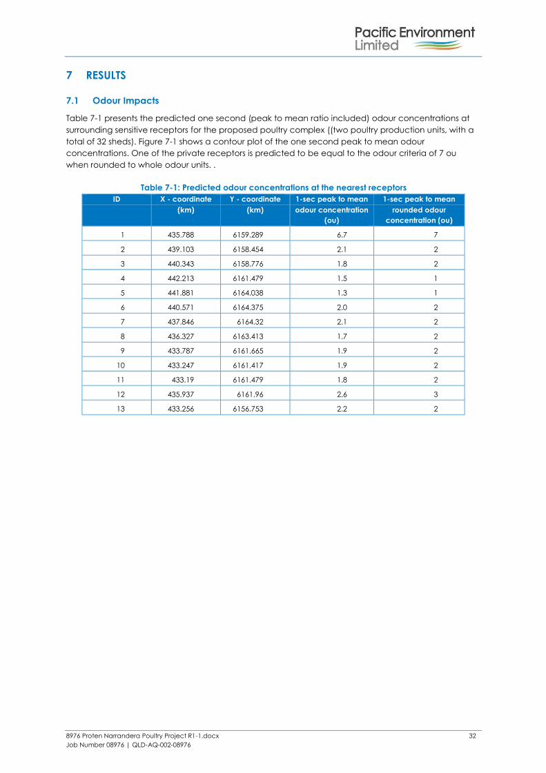
Table 7-1 presents the predicted one second (peak to mean ratio included) odour concentrations at

surrounding sensitive receptors for the proposed poultry complex ((two poultry production units, with a

total of 32 sheds). Figure 7-1 shows a contour plot of the one second peak to mean odour

concentrations. One of the private receptors is predicted to be equal to the odour criteria of 7 ou

when rounded to whole odour units. .

Table 7-1: Predicted odour concentrations at the nearest receptors

ID X - coordinate Y - coordinate 1-sec peak to mean 1-sec peak to mean

(km) (km) odour concentration

(ou)

rounded odour

concentration (ou)

1 435.788 6159.289 6.7 7

2 439.103 6158.454 2.1 2

3 440.343 6158.776 1.8 2

4 442.213 6161.479 1.5 1

5 441.881 6164.038 1.3 1

6 440.571 6164.375 2.0 2

7 437.846 6164.32 2.1 2

8 436.327 6163.413 1.7 2

9 433.787 6161.665 1.9 2

10 433.247 6161.417 1.9 2

11 433.19 6161.479 1.8 2

12 435.937 6161.96 2.6 3

13 433.256 6156.753 2.2 2



Figure 7-1: Predicted 1-second peak-to-mean concentration

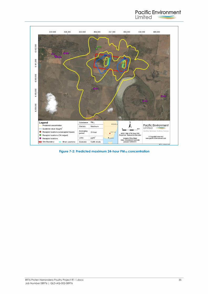
7.2 Particulate Matter

Table 7-2 presents a summary of the predicted PM10 levels at the nearest sensitive receptor, due to the

operations of the Project alone. Figure 7-2 and Figure 7-3 show the predicted 24-hour maximum and

annual average PM10 levels respectively. Modelling results show that maximum 24 hour and annual

average PM10 are below the respective assessment criterion at the sensitive receptors. At the boundary

of the property the maximum 24 hour PM10 concentration exceeds the 50 µg/m3 assessment criterion.



Table 7-2: Predicted PM10 concentrations at the nearest receptors

ID X - coordinate Y - coordinate Max 24-hr PM10 Annual avg PM10

(km) (km) (µg/m3) (µg/m3)

1 435.788 6159.289 20 0.57

2 439.103 6158.454 2.7 0.14

3 440.343 6158.776 2.2 0.11

4 442.213 6161.479 1.7 0.08

5 441.881 6164.038 2.0 0.08

6 440.571 6164.375 3.7 0.16

7 437.846 6164.320 4.2 0.18

8 436.327 6163.413 6.4 0.18

9 433.787 6161.665 5.4 0.15

10 433.247 6161.417 7.2 0.15

11 433.190 6161.479 6.6 0.14

12 435.937 6161.960 17 0.30

13 433.256 6156.753 3.3 0.14



Figure 7-2: Predicted maximum 24-hour PM10 concentration



Figure 7-3: Predicted annual average PM10 concentration

7.3 Cumulative Assessment

7.3.1 Odour

It is not always practical to assess the cumulative odour impact of all odour sources that may impact

on discrete receptors. However, it is common in odour assessments to assess the incremental increase

in odour from a proposed development against the assessment criteria, particularly where no other

sources of similar odour character are present.

As there are no farms within 10 kilometres we have not performed a cumulative assessment for odour.

7.3.2 Annual average PM10

The highest annual average PM10 concentration measured at the EPA Albury monitoring station was

recorded in 2007 with a result of 21 µg/m3 (see Section 4.2). When this value is added to the annual

average PM10 prediction at the closest receptor (R1) the cumulative value would be 22.1 µg/m3 which

is below the EPA assessment criterion of 30 µg/m3.

7.3.3 24 hour average PM10

Cumulative 24-hour PM10 impacts (i.e. assuming rural areas have other agricultural dust sources) have

been evaluated using a statistical approach (Monte Carlo Simulation) focussing on the sensitive

receptors nearest the development. The Monte Carlo Simulation is a statistical approach that

combines the frequency distribution of one data set (in this case, measured 24-hour average PM10

concentrations representative of the site) with the frequency distribution of another data set (modelled

concentrations at a given receptor). This is achieved by randomly and repeatedly sampling and



combining values within the two data sets to create a third, ‘cumulative’ data set and associated

frequency distribution. To generate greater confidence in the statistical robustness of the results, the

Monte Carlo Simulation was repeated 250,000 times for each of the chosen receptors.

Monte Carlo simulations provide results in terms of the statistical probability that an event may occur.

For this assessment, the results are the statistical probability that a certain concentration of 24-hour

average PM10 concentration will occur in a single one year period (i.e. 365 days).

The results of the Monte Carlo analysis for the six closest receptors are presented graphically in Figure

7-4. The plots show the statistical probability (presented as number of days) of 24 hour average PM10

concentrations being above the NSW EPA 24-hour average PM10 criterion of 50 µg/m3 and also

compares the cumulative probability with the measured background (dashed red line).

Figure 7-4 shows that the background levels are estimated to exceed the criterion on approximately

four days per year. It also shows that the most affected receptor, R1, is not expected to experience

any additional exceedances due to the project as the cumulative ground level concentrations are

largely indistinguishable from background at the 50 µg/m3 levels.

Figure 7-4: Predicted Number of Days Over 24-Hour average PM10 Concentration



8 CONCLUSION

This report has assessed potential odour and dust impacts associated with the proposed ProTen poultry

broiler operation (2 production units) located near Narrandera NSW. Local land use, terrain and

meteorology have been considered in the assessment and dispersion modelling was completed using

CALPUFF.

The predicted odour levels at the nearest receptors are predicted to be below the NSW EPA

assessment criterion of 7 ou.

The predicted PM10 concentrations at the aforementioned receptors are also predicted to be below

the EPA assessment criteria.



9 RECOMMENDATIONS

Based on our assessment we make the following recommendations:

The farm is to be operated and managed in line with Best Practice Management for Meat

Chicken Production in New South Wales - Manual 2 – Meat Chicken Growing Management

(Department of Primary Industries, 2012).

A vegetative buffer is to be established around the perimeter of the sheds to enhance the

dispersion of air emitted from the sheds, and to assist in filtering airborne particles.

Thought be given to installing a weather station on site at a suitable location.



10 REFERENCES

Australian Poultry CRC, 2011. Dust and odour emissions from meat chicken sheds, Armidale: Australian

Poultry CRC.

Clarkson, C. R. & Misselbrook, T. H., 1991. Odour Emissions from Broiler Chickens. in: V.C. Nielsen, J.H.

Voorburg, P. L'Hermite (Eds.), Odour and Ammonia Emissions from Livestock Farming (Proceedings of a

seminar held in Silsoe, UK 26-28 March 1990).. London, Elsevier Science Publishers.

DAFF, 2012. Queensland Guidelines Meat Chicken Farms, Brisbane: Department of Agriculture, Fisheries

and Forestry, State of Queensland.

Department of Primary Industries, 2012. Best Practice Management for Meat Chicken Production in

New South Wales - Manual 2 – Meat Chicken Growing Management, Sydney : Department of Primary

Industries.

Hurley P, 2008a. TAPM V4 User Manual - CSIRO Marine and Atmospheric Research Internal Report No.5

Aspendale, Victoria: CSIRO Marine and Atmospheric Research, s.l.: s.n.

Hurley P, 2008b. TAPM V4 Part 1: Technical Description - CSIRO Marine and Atmospheric Research

Paper No. 25 Aspendale, Victoria: CSIRO Marine and Atmospheric REsearch, Canberra: CSIRO .

Hurley P, 2008c. TAPM V4 Part 2: Summary of Some Verification Studies - CSIRO Marine and Atmospheric

Research Paper No. 26 Aspendale, Victoria: CSIRO Marine and Atmospheric Research, Canberra:

CSIRO .

Katestone Scientific, 1995. The Evaluation of peak-to-mean ratios for odour assessments, Brisbane:

Katestone Scientific .

Katestone Scientific, 1998. Report from Katestone Scientific to Environment Protection Authority of NSW,

Peak to Mean Ratios for Odour Assessments, Brisbane: Katestone Scientific.

Mirrabooka, 2002. "Silverweir" Broiler Farm Development Approval Application, Air Quality Impact

Assessment, Brisbane: Mirrabooka Consulting.

NSW EPA, 2005. Approved Methods for the Modelling and Assessment of Air Pollutants in NSW. s.l.:s.n.

NSW EPA, 2006. Assessment and management of odours from stationary sources in NSW. s.l.:s.n.

NSW OEH, 2011. Generic Guidance and Optimum Model Settings for the CALPUFF modelling system for

inclusion into the 'Approved methods for the Modeling and Assessment of Air Pollutants in NSW,

Australia', Sydney: Offices of Environment and Heritage, New South Wales.

Ormerod, R. & Holmes, G., 2005. Description of PAE Meat Chicken Farm Odour Emissions Model,

Brisbane: Pacific Air & Environment.

PAEHolmes, 2011. Best Practice Guidance for the Queensland Poultry Industry - Plume Dispersion

Modelling and Meteorological Processing, Bribane: PAEHolmes .

PAEHolmes, 2012. Environmental Evaluation - Monarch Nominees - Ford Road Farm, Brisbane:

PAEHolmes.

Scire, J. S., Strimaitis, D. G. & Yamartino, R. J., 2000. A users guide for the CALPUFF Dispersion Model

(Version 5), Concord MA: Earth Tech Inc.



Standards Australia, 2001. AS4323.3 Determination of Odour Concentration by Dynamic Olfactometry.

Sydney: Standards Australia.

TRC, 2006. CALPUFF Version 6 User's Instructions. May 2006, Lowell, MA, USA: TRC Environmental Corp.

Documents

Odour Assessment – Narrandera Poultry Project – Farm 1 F... · report odour assessment – narrandera poultry project – farm 1 proten holdings pty limited job id. 08976 5 september