Ocean Initialization for Seasonal Forecasts

M. A. Balmaseda 1, O. Alves2, A. Arribas3, T. Awaji4, D. Behringer5, N. Ferry6, Y. Fujii7 , T. Lee8, M.Rienecker9, T. Rosati10, D. Stammer11

1European Centre for Medium Range Weather Forecasts, Reading UK2 Centre for Australian Weather and Climate Research (CAWCR), Melbourne, Australia

3UK Met Office, Exeter, UK4 Japan Agency for Marine-Earth Science and Technology (JAMSTEC), Yokohama, Japan

5NCEP, Camp Springs, MD,USA6 Mercator-Ocean, Ramonville St Agne, France

7Oceanographic research Department, Meteorological Research Institute, Tsukuba, Japan8NASA Jet Propulsion Laboratory, California Institute of Technology, Pasadena, CA, USA

9Global Modeling and Assimilation Office, NASA Goddard Space Flight Center, Greenbelt, USA10NOAA/GFDL, Princeton, USA

11Institut für Meereskunde, University of Hamburg, Germany

Corresponding author: Magdalena A. Balmaseda, ECMWF, Shinfield Park, Reading RG2 9AX, UK,(Magdalena.Balmaseda@ecmwf.int)

Abstract

The potential for climate predictability at seasonal time scales resides in information provided bythe ocean initial conditions, in particular the upper thermal structure. Currently, severaloperational centres issue routine seasonal forecasts produced with coupled ocean-atmospheremodels, requiring real-time knowledge of the state of the global ocean. Seasonal forecastingneeds the calibration of the numerical output of the coupled model, which in turn requires anhistorical ocean reanalysis, as will be discussed in this paper.

Assimilation of observations into an ocean model forced by prescribed atmospheric fluxes is themost common practice for initialization of the ocean component of a coupled model. It is shownthat the assimilation of ocean data reduces the uncertainty in the ocean estimation arising fromthe uncertainty in the forcing fluxes. Although data assimilation also improves the skill ofseasonal forecasts in many cases, its impact is often overshadowed by errors in the coupledmodels. This paper offers a review of the existing ocean analysis efforts aiming at theinitialization of seasonal forecasts. The current practice, known as "uncoupled" initialization, hasoften been criticized as having several shortcomings, the initialization shock being one of them.On the other hand, the uncoupled initialization usually benefits from better knowledge of theatmospheric forcing fluxes, an advantage that should not be overlooked.

In recent years, the idea of obtaining truly "coupled" initialization, where the differentcomponents of the coupled system are well balanced, has stimulated several research activitiesthat will be reviewed in light of their application to seasonal forecasts.

Key words: Seasonal forecasts, initialization, ocean reanalysis, data assimilation.

1.IntroductionSeasonal forecasting is now a routine activity in several operational centers around the world. Seasonalforecasting systems are based on coupled ocean-atmosphere general circulation models that predict boththe lower boundary conditions (namely sea surface temperatures (SSTs)) and their impact on theatmospheric circulation. This approach is often called a one-tier approach. In a one-tier approach,forecasting the SST using a fully-coupled model is essentially an initial value problem since predictabilitylargely resides in the initial state of the ocean. The probabilistic nature of seasonal forecasting is

addressed by performing an ensemble of integrations with the aim of sampling the probability densityfunction (PDF), primarily for the atmosphere. The uncertainty in the ocean initial conditions should beconsidered in the ensemble generation (Vialard et al. 2003). Because of deficiencies in the componentmodels the coupled model drifts with forecast lead time towards the biased coupled model climate. Acommon approach is to remove the drift a posteriori: a set of historical hindcasts is performed to providean estimate of the model climatological PDF, which is then used for a-posteriori calibration of theforecast results. The quality of seasonal forecasts is determined by the various elements of the forecastingsystem (the ocean initialization, the coupled model, the ensemble generation and the calibration strategy),all of which are closely interrelated. The interdependence of the different elements becomes clear whenconsidering the calibration procedure. The a-posteriori calibration of model output requires an estimate ofthe model climatology, which is obtained by performing a series of coupled hindcasts during somehistorical period (typically 15-25 years). A historical record of hindcasts is also needed for skillassessment. Ocean initial conditions spanning the chosen calibration period, equivalent to an ocean“reanalysis” of the historical data stream, are then required. The interannual variability represented by theocean reanalysis will have an impact on both the calibration and on the assessment of the skill.

The skill of the seasonal forecasts is often used to gauge the goodness of the ocean initial conditionsalthough that may not always be an appropriate measure: the quality of the coupled model will determinethe precision of the assessment - if the major source of forecast error comes from the coupled model,changes to the ocean initial conditions would have little impact on the forecast skill. This is something tobear in mind when interpreting results of the impact of the ocean data assimilation on seasonal forecasts.

Although ocean data assimilation is now commonly used to generate ocean initial conditions for seasonalforecasts, the procedure is not without issues. For instance, the assimilation can improve the forecasts bycorrecting the mean state, but it can also introduce problems such as initialization shock. The non-stationary nature of the ocean observing system can degrade the interannual variability of the ocean initialconditions if not treated carefully (Balmaseda et al. 2007). This paper discusses the potential benefits andproblems induced by ocean data assimilation, mainly due to the existence of systematic biases in thecoupled system. The paper is organized as follows. Section 2 offers a brief description of the initializationprocedures used in operational seasonal forecasts. The impact of data assimilation in the creation of theinitial conditions and in the seasonal forecasts is presented in sections 3 and 4. A brief review of recentinitiatives towards a second generation of initialization procedures aiming at a balance initialization isoffered in section 5. The paper ends with a summary and main conclusions.

2 Overview of initialization in existing seasonal forecasting systemsMost seasonal forecast systems have a separate initialization of the ocean and atmospheric components ofthe coupled system, aiming at generating the best analyses of the atmosphere and ocean throughcomprehensive data assimilation schemes in both media. This is the strategy followed in the operationalor quasi-operational seasonal forecasting systems listed in table 1 and described briefly below. It is alsothe most common strategy followed in most of the coupled integrations in several research projects, suchas DEMETER and ENSEMBLES, which will not be described in this paper.

The production of seasonal forecasts is expensive: the need for ensembles and calibration implies theintegration of the coupled model for several hundreds of years. This computational burden limits thepractical resolution of the ocean model, which is typically of the order of 1 degree with some equatorialrefinement in the horizontal, and about 10 meters in the vertical in the upper ocean. The emphasis is onthe initialization of the upper ocean thermal structure, particularly the tropics, where the ocean has astrong driving influence on the atmospheric circulation. The atmospheric analysis in turn has very strongimpact on the quality of the ocean analysis since it provides the fluxes used to drive the ocean model inthe production of the first guess. The atmospheric fluxes are usually provided by an atmospheric re-analysis system (ERA40, JRA-25, NCEP), and as these are usually limited in duration, the fluxes fromthe operational analysis are then used (ops in table 1). A key parameter in the ocean analysis is SST. It isone of the better-observed variables and the ocean analysis usually does not modify this field greatly.

MRI-JMA http://ds.data.jma.go.jp/tcc/tcc/products/elnino/index.htmlOperationalMOVE/MRI.COM-G (1x1 +0.3eq) .50

vertical levelsMulti-variate 3DVARJRA-25(1979-2003)+JMA ops fluxes10 days assimilation cycle+IAU

COBE-SST gridded productSubsurface T&S (GTS+)SLA along track from AVISOMDT analyzed with historical T, S

Weighted mean of clim. (1%)and model fields is used for FG..

From 1979 onwardsBoth Delayed (34-38 days) and

NRT (3-7 days)Lagged ensemble

ORA-S3 (ECMWF) www.ecmwf.int/ products/forecasts/d/charts/oceanECMWF System 3 http://www.ecmwf.int/products/forecasts/d/charts/seasonal/OperationalHOPE (1x1+0.3 eq). 29 vertical levelsMultivariate OIERA40 (1959-2002)+ ECMWFops fluxes10 day assim cycle+IAU

HadISST+ Reynolds OI v2 SSTSubsurface T&S

(ENACT/ENSEMBLES+GTS)SLA maps from AVISOMDT by assimilating T,S

Bias correction (T,S andPressure)

10-year relaxation to climFrom 1959 onwardsBoth Delayed (12 days) and RT5-analyses ensemble

POAMA – PEODAS (CAWCR, Melbourne)In transition to OperationsACOM-2 Ocean Model Based on MOM2.ERA-40 (1980-2001)+NCEP2 (2002

onwards) fluxes3 Day assimilation cycleMulti-variate ensemble OI

ENACT observational data set T&SSST from NCEP re-analysisTime evolving covariances from

ensemble perturbed about mainanalysis using forcing perturbations

T&S 3D relaxation to Levituswith 2year time scale

Ensemble initial conditions fromensemble of states used forcovariance calculation

GODAS (NCEP) http://www.cpc.ncep.noaa.gov/products/GODAS/OperationalMOMv3 (1x1 + 1/3 at eq). 40 vertical

levels, 3DVarNCEP/DOE R2 atmospheric fluxes12 hour assimilation cycle+IAU

Temperature from NODC,GTSPPand GTS.

Along Track SLA from Jason-1SST from Reynolds OIv2.MDT by assimilation of T,S

From 1979 onwardsBoth 14 days and 1 day lags

relative to RTNo relaxation to climate

MERCATOR (Meteo France) http://bulletin.mercator-ocean.fr/html/welcome_en.jspOperationalOPA8.2 ORCA2 (2cosx 2° + 0.5° eq.)

reduced order Kalman Filter (SEEK)ERA-40 (1979-2001) + ops fluxes7-day assimilation cycle

Reynolds OI v2 SSTSubsurface T&S

(ENSEMBLES+CORIOLIS)SLA along track from AVISOModel MDT

10-year relaxation to climFrom 1979 onwards7 days behind RT

MO (MetOffice) http://www.metoffice.gov.uk/research/seasonal/OperationalHadOM3/OI (1x1+0.3 eq)ERA40 (1985-2002)+ ECMWFops fluxes7 days assim cycle+IAU

HadISST+ Reynolds OI v2 SSTSubsurface T&S

(ENACT/ENSEMBLES+GTS)

Bias correction (Pressure)From 1985 onwards3 days behind RT5-analyses ensemble

GMAO ODAS-1 http://gmao.gsfc.nasa.gov/research/oceanassim/ODA_vis.phpGMAO Seasonal Forecasts: http://gmao.gsfc.nasa.gov/cgi-bin/products/climateforecasts/index.cgiOperationalPoseidon/OI and EnKF (5/8 x 1/3)NCEP R1+ SSMI winds GPCP precip5 day assim cycle+IAU

Reynolds OI v2 SSTSubsurface T&S (NCEP GTS + TAO

+ GDAC Argo)SLA along-track from JPL (EnKF

only)Online bias correction for MDT

(EnKF only)

Bias correction (SLA)From 1993 onwardsDelayed (about 7 days)3-analyses ensemble

Table1: Summary of different ocean assimilation systems used in the initialization of operational andquasi-operational seasonal forecasts.

Most of the initialization systems also use subsurface temperature, most recently also salinity (mainlyfrom Argo), and altimeter derived sea-level anomalies (SLA). The latter usually needs the prescription of

an external Mean Dynamic Topography (MDT). Some of the initialization systems may use an on-linebias correction scheme or relaxation to climatology to control the mean state.

2.1 MRI-JMAThe Japan Meteorological Agency (JMA) provides operational information of the real time state of theocean and atmosphere in the tropical Pacific associated with ENSO. JMA has also forecast the anomaliesof the monthly mean SST in the NINO3 region (5ºS-5ºN, 90-150ºW) since March, 2008(http://ds.data.jma.go.jp/tcc/tcc/products/elnino/ index.html). These products are based on a dataassimilation system, MOVE/MRI.COM-G (Usui et al. 2006), and a coupled ocean-atmosphere generalcirculation model, JMA/MRI-CGCM (Yasuda et al. 2007). MOVE/MRI.COM-G is the global dataassimilation system composed of the ocean model, MRI.COM (Ishikawa et al. 2005), and the oceananalysis scheme, MOVE (Fujii and Kamachi 2003; Fujii et al. 2005). The model uses a near-globaldomain (75ºS-75ºN) and 50 levels in the vertical. The grid spacing is 1º, with meridional equatorialrefinement to 0.3º within 5ºS-5ºN. The layer thicknesses are less than 10m above 200m depth. Theanalysis scheme, MOVE, adopts a multivariate 3-Dimesional Variational (3DVAR) method with verticalcoupled Temperature-Salinity (T-S) Empirical Orthogonal Function (EOF) modes. A nonlinearobservation operator for SLA data, a constraint avoiding density inversion, and a variational qualitycontrol procedure is adopted. The optimal temperature and salinity fields analyzed in MOVE are insertedinto the model using the Incremental Analysis Updates (IAU) technique (Bloom et al. 1996), using anassimilation cycle of 10 days.

MOVE/MRI.COM-G assimilates satellite SLA data from AVISO (http://www.aviso. oceanobs.com),the gridded COBE-SST (Ishii et al. 2005), and in situ temperature and salinity profiles. In reanalyses,temperature and salinity profiles are obtained from the World Ocean Database 2001 (WOD01; Conkrightet al. 2002), the Global Temperature-Salinity Profile Program (GTSPP) database (Hamilton 1994), andthe data of the TAO/TRITON array (Hayes et al. 1991; McPhaden et al. 1998; Kuroda 2002). For the realtime analyses, the in-situ data is acquired via the GTS and some domestic sources (in Table 1)

2.2 ECMWF ORA-S3The ECMWF Ocean Reanalysis System ORA-S3 (Balmaseda et al. 2008a) has been operational sinceAugust 2006, providing ocean initial conditions for the ECMWF seasonal and monthly forecasts sinceMarch 2007. The ocean data assimilation system for ORA-S3 is based on the HOPE-OI scheme. Theocean model has a horizontal resolution of 1º with equatorial refinement ( 0.3º meridional resolutionwithin 5º of the equator).The first guess is obtained by forcing the ocean model with daily fluxes ofmomentum, heat and fresh water from the ERA-40 reanalysis (Uppala et al. 2005) for the period January1959 to June 2002 and NWP operational analyses thereafter. The ORA-S3 system uses a 3D OptimalInterpolation (OI) scheme to assimilate temperature, salinity, altimeter derived sea-level anomalies andglobal sea level trends. The assimilation of altimeter is described in Vidard et al. 2008. Physicalconstraints relate the temperature and salinity increments (Troccoli et al. 2002.), density and velocityincrements (Burgers et al. 2002) and sea level and vertical profile displacement (Cooper and Haines1996). The background temperature, salinity and pressure gradient are bias corrected following thealgorithm described in Balmaseda et al. 2007. A selection of historical and real-time ocean analysisproducts can be seen at www.ecmwf.int/ products/forecasts/d/charts/ocean. The subsurface observationscome from the quality-controlled dataset prepared for the ENACT and ENSEMBLES projects until 2004(Ingleby and Huddleston, 2006), and from the GTS thereafter (ENACT/GTS). The altimeter data used areglobal gridded weekly maps from 1993 onwards (Le Traon et al., 1998). The model SSTs are stronglyrelaxed to analyzed daily SST maps from the OIv2 SST product (Reynolds et al., 2002) from 1982onwards. Prior to that date, the same SST product as in the ERA-40 reanalysis was used.

In ORA-S3, the introduction of a bias correction algorithm with both prescribed and adaptive componentshas improved the representation of the inter-annual variability of the upper ocean heat content. However,there may still be problems with the representation of the variability in very poorly observed areas such asthe Southern Ocean and also in the salinity field. ORA-S3 consists of an ensemble of five simultaneous

reanalyses, aiming at sampling uncertainty in the ocean initial conditions, and thereby contributing to thecreation of the ensemble of forecasts for the probabilistic predictions at monthly and seasonal ranges.

2.3 MERCATOR-Meteo FranceMercator-Ocean has provided ocean initial conditions for the Météo-France ocean-atmosphere coupledsystem since September 2004. These ocean initial conditions are produced with PSY2G2 operationalocean analysis / forecasting system based on the OPA8.2 ocean model (ORCA2 model configuration,Madec et al. 1998) and on a reduced order Kalman filter data assimilation scheme. The ocean model has ahorizontal resolution of 2.cosx 2° with an equatorial meridional refinement of ~0.5° resolution near theequator.The ocean model is forced with daily fluxes of momentum, heat and fresh water from the ERA-40reanalysis for the period January 1979 to December 2001 and from the operational analysis thereafter. Itassimilates subsurface temperature and salinity, SLA data and SST maps. The subsurface data comesfrom the ENACT/ENSEMBLES data base until 2001. Afterwards, data are quality controlled andprovided by the CORIOLIS data center (http://www.coriolis.eu.org) both in delayed mode and real-time.The altimetric data are along-track SLA provided from November 1992 onwards by SSALTO/DUACS.The assimilated SST product is used as boundary conditions in the atmospheric analyses subsequentlyused to force the ocean model (ERA-40 and ECMWF operational analyses after 2001).

The data assimilation scheme is a reduced order Kalman filter based on the SEEK formulation (Pham etal. 1998). The control vector is composed of the temperature and salinity fields and the barotropic height.The forecast error covariance is based on the statistics of a collection of 3D ocean state anomalies(typically a few hundred) and is seasonally variable. In this case, the anomalies are high pass filteredocean states available over the period 1992-2001 sampled every 3 days. The analysis producestemperature and salinity as well as barotropic velocity increments. Physical balance operators are used todeduce zonal and meridional velocity fields from these increments.

2.4 POAMA – PEODAS (CAWCR)The Predictive Ocean Atmosphere Model for Australia (POAMA) is a dynamical seasonal predictionsystem developed by the Centre for Australia Weather and Climate Research (CAWCR: an adjunctcentre of the Australian Bureau of Meteorology and CSIRO). One of the major new developments inPOAMA is a new ocean data assimilation system called PEODAS (POAMA Ensemble Ocean DataAssimilation System. The system is based on multivariate ensemble Optimum Interpolation (Oke et al.2005) where the background error covariance is calculated from an ensemble of ocean states. Unlike Okeet al. (2005) which uses a static ensemble, PEODAS uses a time evolving ensemble to calculate a timedependent multivariate error covariance matrix. An ensemble is run in parallel to the main analyses byperturbing the ocean model forcing about the main analysis run, using a method developed by Alves andRobert (2005).

An ocean re-analysis has been conducted from 1977 to 2007, assimilating temperature and salinityobservations from the ENACT/ENSEMBLE project. During the assimilation, temperature and salinitywere relaxed to monthly climatology through the water column with an e-folding time scale of 2 years.The model SST was strongly nudged to the SST product from the NCEP re-analysis with a 1-day timescale.

2.5 NCEPThe NOAA/NCEP Global Ocean Data Assimilation System (GODAS) (Behringer, 2007) was developedas a replacement for the earlier Pacific Ocean system and was made operational in 2003. It has providedthe oceanic initial conditions for seasonal and interannual forecasting with the NCEP coupled ClimateForecast System (CFS) (Saha et al., 2006) since 2004. The GODAS is based a quasi-global configurationof the GFDL MOMv3. The model domain extends from 75OS to 65ON and has a resolution of 1O by 1O

enhanced to 1/3O meridionally within 10O of the equator. The model has 40 levels with a 10 meterresolution in the upper 200 meters. The GODAS is forced by momentum, heat and fresh water fluxes

from the NCEP/DOE atmospheric Reanalysis 2 (R2) (Kanamitsu et al. 2002) which is maintainedoperationally at NCEP. In addition to the R2 forcing, the temperature at the top model level is relaxed to aweekly OI analysis of sea surface temperature (Reynolds et al., 2002) and the surface salinity is relaxed toan annual climatology. The assimilation method is a 3DVAR scheme derived from the work of Derberand Rosati (1989). Some of the improvements that have been made include the incorporation of revisedbackground error covariances that allow for spatial and temporal variation of the local error variance(Behringer et al. 1998) and the assimilation of satellite altimetry data (Vossepoel and Behringer, 2000;Behringer, 2007). The GODAS assimilates temperature profiles from XBTs, from TAO, TRITON andPIRATA moorings and from Argo profiling floats (The Argo Science Team, 2001). For use in oceanreanalysis, XBT observations made prior to 1990 have been acquired from the NODC World OceanDatabase 1998 (Conkright et al., 1999), while XBTs made subsequent to 1990 have been acquired fromthe Global Temperature-Salinity Profile Project (GTSPP) (Hamilton, 1994). For use in operations,temperature profile data are acquired via the GTS. The GODAS also assimilates synthetic salinityprofiles which are computed for each temperature profile using a local T-S climatology based on theannual mean fields of temperature and salinity from the NODC World Ocean Database. Finally, theGODAS assimilates along-track Jason-1 altimetry data that NCEP receives through a direct link from theUS Naval Oceanographic Office in the form of Interim Geophysical Data Records. Only the variable partof the altimetry is assimilated. The variability of the altimetry is determined relative to the 1993-1999mean of a consolidated TOPEX/Jason-1 data set. The mean dynamic topography (MDT) of the model iscomputed for the same time period from a GODAS run that assimilates only temperature and salinity.Products derived from the GODAS can be found at www.cpc.ncep.noaa.gov/products/GODAS/.

2.6 Met OfficeThe Met Office seasonal ocean data assimilation system has been operational since March 2004 toprovide ocean initial conditions for the Met Office seasonal forecasting system (GloSea3). Theassimilation uses an optimal interpolation scheme based on the ocean component of the GloSea modelwhich has a horizontal resolution of 1º with equatorial refinement (0.3º meridional resolution within 5º ofthe equator). The first guess is obtained by forcing the ocean model with daily fluxes of momentum, heatand fresh water from the ERA-40 reanalysis for the period January 1985 to June 2002 and ECMWF’sNWP operational analysis thereafter. It assimilates subsurface temperature and salinity. The subsurfaceobservations come from the quality-controlled dataset prepared for the ENACT and ENSEMBLESprojects until 2004, and from the ENACT/GTS. The model SSTs are strongly relaxed to analyzed dailySST maps from the OIv2 SST product.

2.7 GMAOThe GMAO Ocean Data Assimilation System Version 1 (ODAS-1), using an Ensemble Kalman Filter(EnKF, Keppenne et al . 2008) has been operational since 2005, providing ocean initial conditions for theGMAO seasonal forecasts since March 2007. The ODAS-1 system using univariate OI has providedinitial conditions for seasonal forecasts since 2000. The ocean model domain is almost global, having asponge layer boundary at 72ºN and at the Strait of Gibraltar. The horizontal resolution is 5/8º zonally and1/3º meridionally, and there are 27 quasi-isopycnal vertical layers. The first guess is obtained by forcingthe ocean model with daily fluxes of heat from the NCEP CDAS1 reanalysis, with momentum from anSSM/I analysis until 2002 and a QuikSCAT analysis after September 2002, and with monthly meanfreshwater fluxes using GPCP. The ocean analyses have been generated from January 1993 to thepresent. The systems assimilate subsurface temperature and salinity, including synthetic salinity derivedfor temperature using a T-S climatology. The subsurface observations come from GTS data quality-controlled by Dr. David Behringer of NOAA/NCEP, from the TAO data portal, and from the ArgoGDAC at FNMOC. The altimeter data from the JPL/PODAAC are assimilated as along-track data from1993 onwards in the EnKF. The model SSTs are strongly relaxed to analyzed daily SST maps from theOIv2 SST product and the model sea surface salinity is relaxed to the Levitus-Boyer climatology.

The ODAS-1 OI is implemented both with a salinity correction scheme following Troccoli and Haines(1999) and with a univariate assimilation of synthetic and Argo salinity profiles in addition to the

univariate assimilation of temperature profiles (e.g., Sun et al., 2007). The ODAS-1 EnKF systemincludes an on-line bias correction algorithm for the assimilation of altimeter data (Keppenne et al.,2005). A selection of historical and real-time ocean analysis products can be seen athttp://gmao.gsfc.nasa.gov/research/oceanassim/ODA_vis.php.

The GMAO seasonal forecasts using the CGCMv1 are initialized with all three analyses. In addition,perturbed analyses are generated for the analysis with the Troccoli-Haines salinity correction, by merelyadding small perturbations according to analyses close to the central time of the forecast initialization. Anadditional multivariate analysis has also been tested based on coupled bred vectors and shows promise forcapturing the state-dependent covariances relevant to the coupled problem and for improving the forecastskill (Yang et al., 2008).

3 Impact of assimilation on the ocean initial conditions

The simplest technique for ocean initialization is to run an ocean model forced with observed wind stressand with a strong relaxation of the model SST to observations. Such stand-alone integrations are referredto as control runs (CNTL) in what follows. This technique would be satisfactory if errors in the forcingfields and ocean model were small. However, surface flux products, even wind stress, as well as oceanmodels are known to have significant errors.

Figure 1: Averaged temperature in the upper 300m in the Equatorial Atlantic region resulting from ocean modelintegrations forced by fluxes from ERA15/OPS (red) and ERA40 (blue) . The upper panel shows the results fromthe CNTL integration, i.e., without data assimilation. The large uncertainty in the ocean state can be reduced byassimilating ocean data (lower panel).

The uncertainty induced in the ocean state can be measured by using a different wind product to force thesame ocean model. Figure 1a shows the evolution of the upper heat content anomalies, as measured bythe averaged temperature in the upper 300m (T300) in the equatorial Atlantic (5N-5S) from two differentCNTL integrations using the ECMWF ocean model. The red line shows the results from the run forced byERA15/OPS winds, while the red line shows results from the run that uses ERA40 winds. The differencesin upper ocean heat content are of the same order as the interannual variability. Figure 1b shows the same

Equatorial Atlantic: T300 anomalies. No assimilation

Equatorial Atlantic: T300 anomalies. Assimilation

diagnostics when data assimilation is included. These results demonstrate that in order to constrain theinterannual variability of the ocean it is necessary to use some data assimilation.

A different question is whether the data assimilation not only constrains the solution, but improves theestimation of the ocean, both mean state and variability. A first test is to verify that the assimilationimproves the fit to the observations used. A more stringent test is to verify against independent data, suchas velocity, which is usually not assimilated. As an example, figure 2 shows how different ocean analysesfit the TAO temperature, salinity and zonal current , in terms of the root mean square (RMS) error ofinter-annual anomalies for the full period that the measurements were available (different for eachvariable). Shown are the PEODAS analysis (black line), the ECMWF ORA-S3 (red line), and a controlintegration, a re-analysis using the PEODAS configuration but without assimilating any sub-surface data(blue line). Also shown is the old POAMA ocean analysis, a predecessor of PEODAS. Both temperatureand salinity data from TAO moorings were assimilated in PEODAS and ECMWF ORA-S3. No currentdata was used in any case, so comparison with the TAO mooring measures how well a balanced state is

Figure 2. RMS error of interannualanomalies of (a) temperature, (b) salinity and(c) zonal current. Shown are the PEODASreanalysis (black), the old POAMA re-analysis (green), the ECMWF ORA-S3 (red)and the Control simulation (blue). Theverifying observations are from the TAOmooring at location 165E.

being produced by the assimilation. The control integration has the same relaxation to sub-surface T andS as PEODAS, which helps to maintain a reasonable mean state (in other studies the integrations used ascontrols that did not have this relaxation). The old POAMA ocean data assimilation system is a univariate2-dimensional OI, which assimilate temperature observations only using static Gaussian covariances as inSmith et al. (1991). There are other differences between POAMA and PEODAS: the relaxation tosubsurface climatology (none in POAMA), the forcing fluxes (NCEP-1 in POAMA and ERA40 inPEODAS), and different physics in the ocean model.

The differences between the PEODAS and POAMA in figure 2 illustrate the advances in dataassimilation in recent years. POAMA exhibits the typical behaviour of the first generation of oceananalysis: improved fit to the assimilated observations (temperature in figure 2a) compared to CNTL, butdegraded fit to the salinity and velocity data (figures 2b and c). More recent assimilation systems (allthose described in section 2, although in the figure 2 only PEODAS and ECMWF are shown) usephysical constraints between temperature and salinity, and between density and currents. Most of thecurrent analysis systems also assimilate salinity, which leads to considerable improvements in the salinityfield (figure 2b). The importance of the balance relationship between temperature and salinity for therepresentation of the barrier layer is discussed below. In the new assimilation systems, the equatorialcurrents are not particularly degraded, being comparable to the CNTL integration. This is probably theresult of several contributions: multivariate constraints, improvement in ocean models and in forcingfluxes.

3.1 Impact of assimilation in representation of the barrier layer

The impact of the assimilation scheme on the representation of the barrier layer has been discussed byFujii et al. (2008b), using the MOVE assimilation system. MOVE applies vertical coupled T-S EOFmodes as the control variables, which allows consistent correction of the model temperature and salinityfields. In particular, the model salinity field is properly modified with the information from thetemperature correction through the T-S relation even if few salinity observations are available. In order toexamine the effect of the salinity corrections, two types of data assimilation experiments (T+S and NOS)have been performed with MOVE/MRI.COM-G. Temperature and salinity corrections are applied in T+S,while in experiment NOS only the temperature increments are applied.

There is a large difference in the subsurface salinity field in the equatorial Pacific between T+S andNOS (figure 3). High salinity associated with the South Pacific Tropical Water (SPTW) is estimated

Figure 3: Vertical sections of climatological salinity fields along 160ºE (left) and 110ºW (right)between 20ºS and 20ºN in T+S (top) and NOS (bottom). Units are psu.

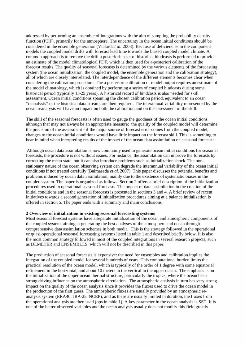
inadequately low in NOS. The moderate vertical contrast of the salinity fields in NOS implies that densityinstability is induced by forced temperature modification without proper salinity adjustment. This is thecommon feature of the conventional assimilation system where temperature field alone is modifiedwithout salinity correction (e.g., Troccoli et al. 2002). The salinity field is however properly reproducedin T+S.

The salinity bias in NOS can degrade the temperature field. Figure 4 shows the variation of the barrierlayer thickness and the difference of the warm water heat content between T+S and NOS at the equator.The warm water heat content is defined as the heat content in the water exceeding 28ºC. The thick barrierlayer is displaced according to the ENSO cycle. It moves to the eastern equatorial Pacific in the large ElNiño period (1997) and temporally disappears after that. The position of large positive difference of warmwater heat content has a good correspondence with the position of thick barrier layer. The barrier layertends to increase the heat content in the warm water by avoiding vertical mixing in T+S. The low salinitybias of SPTW, however, weakens the density stratification caused by vertical salinity gradient, andprevents the formation of a substantial barrier layer, which results in the reduction of warm water heatcontent in NOS. Thus, salinity correction improves the subsurface temperature field by estimating thevertical density stratification properly.

4 Impact of initialization on seasonal forecasts

4.1. Impact of initialization in the ECMWF seasonal forecasting system.Alves et al. (2003) found that data assimilation improved the skill of the seasonal forecasts using oneversion of the ECMWF coupled model. Since the impact of data assimilation is likely to be modeldependent, the same question is revisited in this paper using the results from other seasonal forecastingsystems. The impact of initialization on the mean state, variability and skill of coupled forecasts at

Figure 4: Left: longitude-time section of the barrier layer thickness (m) at the equator in T+S.Right: longitude-time section of the difference of the warm water heat content (kcal·cm2) betweenT+S and NOS (T+S minus NOS) at the equator.

seasonal time scale has been revisited by Balmaseda et al. (2008b), using the latest ECMWF seasonalforecasting system (S3) (Anderson et al. 2007).

There are three experiments where the initial conditions have been produced by (i) the ORA-S3 oceanreanalysis system, (ii) the ocean model forced by the same atmospheric fluxes from reanalysis winds butwithout data assimilation, and (iii) the ocean model forced by atmospheric fluxes produced by theatmospheric model forced by observed SST, as in Luo et al. (2005). In the three cases, SST analyses areused to constrain the ocean initial conditions. In method (i), the coupled system thus starts close to theobserved state but it is not obvious that this leads to the most skillful forecasts as the method can haveundesirable initialization shocks. Method (iii) can reduce the initialization shock since the atmosphere andocean models will be in closer balance at the start of the coupled integrations. The three experiments canalso be seen as observing system experiments. Differences between (i) and (ii) are indicative of theimpact of ocean observations, and comparison of (ii) and (iii) are indicative of the impact of theatmospheric observation that were used to produce the atmospheric reanalysis. In what follows we refer tothese methods as ALL, NO-OCOBS and SST-ONLY experiments.

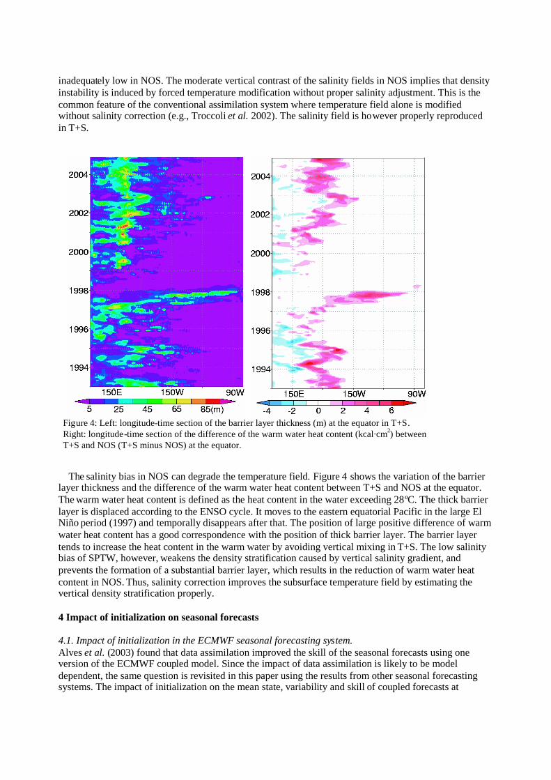
A series of 7-month, 5-member ensemble coupled hindcasts spanning the period 1987-2000, 3 monthsapart, was performed with initial conditions from each method. Figure 5 shows that both the mean stateand the interannual variability are sensitive to the initialization method. In the Eastern Pacific (NINO3,left panel), ALL shows the strongest warm bias, which is symptomatic of the existence of initializationshock: the coupled model is not able to maintain the slope of the thermocline in the initial conditions, andfast dynamic adjustment takes place through a downwelling Kelvin wave. In experiment SST-ONLY themodel drifts into a cold state, likely related to a too shallow thermocline in the initial conditions. The biasis close to zero in experiment NO-OCOBS. In the Central and Western Pacific (NINO4, right panel) thesmallest bias is obtained with experiment ALL, and the worst with experiment SST-ONLY. Theamplitude of the interannual variability seems to be related to the magnitude of the bias. In NINO3, theleast activity occurs in the presence of warm bias, suggestive of convective processes setting an upperlimit to the amplitude of SST. In NINO4 the experiment cold bias is accompanied by too muchvariability, consistent with the upwelling being overestimated in this region.

Figure 6 shows the impact on forecast skill for various regions in table 2. The relative reduction inthe monthly mean absolute error (MAE) resulting from adding information from the ocean and/oratmosphere observations for forecast range 1-3 months (left) and 4-7 months (right). The WesternPacific (EQ3) is the region where the observational information has largest impact: the combined

Figure 5. Top: forecastdrift as a function offorecast lead time for 4start months in regionsNINO3 (left) and NINO4(right) for experimentsALL (red), NO-OCOBS(blue) and SST-ONLY(green).Bottom: variance ratio asa function of lead timefor the same experimentsaveraged over all startmonths.

the information of ocean and atmospheric observations can reduce the MAE more than 50% in thefirst 3 moths. With the exception of the Equatorial Atlantic (EQATL), the best scores are achievedby experiment ALL. This means that for the ECMWF system, the benefits of the ocean dataassimilation and the use of fluxes from atmospheric (re)analyses more than offset problems arisingfrom initialization shock.

Figure 6: Impact of initialization in forecast skill for different regions, as measured by the reduction in meanabsolute error for the forecast range 1-3 months (left) and 4-7 months (right). Solid bars indicate differences areabove the 80% significance level. The comparison is done for the period 1987-2000. Blue indicates the differencesbetween strategy i and ii which differ in the use of ocean observations. Red (ATOBS) indicates differences betweenii and iii, which differ in the use of atmospheric data, while grey (OC+AT) gives differences between i and iii andrepresents the combined impact of atmospheric and oceanic data.

Table 2: Definition of area average indices

NINO12: 10-0ºS, 90-80ºWNINO3 5ºS-5ºN, 90-150ºWNINO34 5ºS-5ºN, 170-120ºWNINO4 5ºS-5ºN, 160ºE-150ºWEQ3 5ºS-5ºN, 150ºE-170ºWNINO-W 0º-15ºN, 130º-150ºE

EQPAC 5ºS-5ºN, 130ºE-80ºWEQIND 5ºS-5ºN, 40º-120ºEWTIO 10ºS-10ºN, 50º-70ºWSTIO 10ºS-0ºN, 90º-110ºEEQATL 5ºS-5ºN, 70ºW-30ºENSTRATL 5ºN-28ºN, 80ºW-20ºE

4.2. Impact of initialization in the POAMA seasonal forecasting system.

In the previous section it was shown that the PEODAS ocean re-analysis is an improvement with respectto the previous POAMA version and with respect to the Control (no data assimilation). This sectionshows that these improvements lead to better forecast skill of SST at seasonal time scales. For each re-analysis a set of hindcasts starting each month from 1980 to 2001 were produced, the individual hindcastsconsisting of three ensemble members each. For the PEODAS re-analysis a 3-member ensemble wasgenerated using the main PEODAS re-analysis and two other perturbed members. For the Control a 3-member ensemble was also generated, however this time by using the same ocean initial conditions (sinceperturbed states were not available) and taking atmospheric initial conditions six hours apart. For the oldPOAMA re-analysis a 3-member ensemble was generated by taking atmospheric initial conditions sixhours apart.

Forecast Range: 1-3 months. Period 1987-2000

-10

0

10

20

30

40

50

60

NIN

O3

NIN

O4

EQ

3

EQ

PA

C

EQ

IND

WTIO

SE

TIO

EQ

ATL

NS

TRATL

(%)

OCOBS ATOBS OC+AT

-10

-5

0

5

10

15

20

25

30

NIN

O3

NIN

O4

EQ

3

EQ

PAC

EQ

IND

WTIO

SE

TIO

EQ

ATL

NS

TRA

TL

(%)

OCOBS ATOBS OC+AT

Reduction (%) in SST forecast errorRange 1-3 months Range 4-7 months.

Figure 7 shows the NINO3 forecast skill with lead time for forecasts from each set of re-analysis. Theskill curves are base on 3-member ensemble means. Forecasts using PEODAS initial conditions showssignificantly more skill than those using the control or the old POAMA assimilation initial conditions..Forecasts using the control initial conditions show skill at least comparable, if not slightly better, thanforecasts using the old POAMA assimilation, which could be related to the results shown in figure 2,comparing the analysis with the TAO observations. While the old re-analysis had a similar fit to observedtemperature as the new re-analysis and control, the old re-analysis showed a considerably worse fit forsalinity and zonal current. This result can be taken as an indication that, for the assimilation to improveforecast skill, it is important to keep the dynamical and physical balance among variables, and thereforeall variables, not just those directly constrained by observations, should show consistent improvement.

4.3 Observing System Evaluation in MRI-JMAObserving System Evaluation (OSE) is essential to demonstrate the necessity for sustaining the

observing system. The effect of assimilating TAO/TRITON array and Argo float data inMOVE/MRI.COM-G and its impact on the JMA seasonal forecasting system has been evaluated by Fujiiet al. (2008). Three assimilation runs (ALL, NTT, NAF) were performed first. All available observationdata is assimilated in ALL. Data from the TAO/TRITON array is excluded in NTT. Data from Argo isexcluded in NAF. Sets of 11-member ensemble forecasts were then started from January 31st, April 26th,July 30th, and October 28th in 2004-2006. The ensemble is generated by adding perturbation to thegridded SST data (COBE-SST) in the last 10-day data assimilation cycle. Figure 8 shows Root MeanSquare Errors (RMSEs) of the 0-6 month forecasts of monthly SST anomalies averaged in differentregions (defined in Table 2). Here, the 0-month forecast refers to the average in the first month of theforecast, and the RMSEs are normalized by the equivalent RMSEs for persistence forecasts. It should benoted that the forecast bias is estimated for each initial month, each lead time, and each experiment, andremoved before calculating RMSEs. The differences of RMSEs between ALL and NTT show thatTAO/TRITON data has relatively large impact on the forecast of NINO3 and NINO34 regions. Thesignificance levels for the hypothesis that ALL has smaller RMSEs are about 90% for both regions. Thus,TAO/TRITON data has a potential for improving the forecast of SST in the eastern equatorial Pacific. Onthe other hand, RMSEs for CTL is smaller than those for NAF in the all regions. The significance level ismore than 70% in all areas other than WTIO, demonstrating that Argo floats are effective andindispensable observations for the prediction of the SST in the tropical Pacific and Indian Oceans. Similarresults have been obtained with the ECMWF seasonal forecasting system (Balmaseda et al. 2008).

Figure 7: Skill in NINO3 SSTforecasts. The red curves arefrom forecasts initialized by theold POAMA assimilation system(different realizations of 3-member ensembles taken fromthe full 10 member ensemble),navy blue uses the PEODAS re-analysis, green uses the controlre-analysis (with no assimilationof sub-surface data).

4.4 MERCATOR-OCEAN & Météo-France

The improvement in seasonal forecast skill is also exemplified byFigure 9 shows the anomaly correlation coefficient of the SST foMercator-Ocean/Météo-France coupled system version 2 and theimprovement between version 2 and 3 is the assimilation of in situIt should also be noted that the model SST is more realistically cowith a realistic error and not simply strongly nudged towards the oatmospheric model can also be responsible for the differences.

0

0,1

0,2

0,3

0,4

0,5

0,6

0,7

0,8

North.Hem

South.Hem.

Global Nino34 Nino3

Figure 9: Improvement of Sea Surface Temperature ACC for bsystem 2 and 3. The ACC is computed for 3 months lead time fo

2007 period.

Significance

NTT

NAF

６１％

７５％

９１％

９５％

８９％

８５％

７２％

７７％

４１％

７２％

６６％

７４％

３９％

５５％

Normarized RMSE (0- 6month)

0.45

0.5

0.55

0.6

0.65

0.7

0.75

NINO12 NINO3 NINO34 NINO4 NINO- W STIO WTIO

RM

SE

ALLNTTNAF

Significance

NTT

NAF

６１％

７５％

９１％

９５％

８９％

８５％

７２％

７７％

４１％

７２％

６６％

７４％

３９％

５５％

Normarized RMSE (0- 6month)

0.45

0.5

0.55

0.6

0.65

0.7

0.75

NINO12 NINO3 NINO34 NINO4 NINO- W STIO WTIO

RM

SE

ALLNTTNAF

Fig. 8: Impact of withholding TAO/TRITON(NTT) and Argo (NAF) from the initializationof seasonal forecasts in the skill of the JMAEl Niño forecasting system. The bars showthe RMSEs of the 0-6 month forecasts ofmonthly SST anomalies averaged in NINO12,NINO3, NINO34, NINO4, NINO-W, STIOand WTIO normalized by the RMSEs ofpersistence forecasts. The seasonal forecastsare for the period 2004-2006 The forecastbias is estimated for each initial month, eachlead time, and each experiment, and removedbefore calculating RMSEs. From Fujii et al .

the experience in Mercator-Ocean.recasts over different regions for the

more recent version 3. The majordata (temperature and salinity fields).

nstrained in system 3 as it is assimilatedbservations. Improvements in the

Nino4

system2

system3

etween Mercator-Ocean/Météo-Francerecasts in winter (D-J-F) over the 1993-

(2008).

4.5 Impact of ECCO Ocean State Estimation on ENSO Forecast

In an early attempt, Dommenget and Stammer (2004) investigated the impact of ocean state estimatesproduced by the Consortium for Estimating the Circulation and Climate of the Ocean (ECCO) onseasonal forecast of tropical Pacific SST and subsurface fields. For that purpose the MIT model was usedin two distinct settings for ENSO simulation and prediction studies. The first setup served as a control runand was a traditional but simple approach to assimilate SST and wind stress fields into a model, whichwas used subsequently for seasonal ENSO forecasts (Barnett et al. 1993). Results from this simple controlrun were compared to similar results that were obtained in a second approach by using a full ocean stateestimation procedure. This procedure used the MIT adjoint model (Marotzke et al. 1999) to obtain asolution of the time-varying ocean on a 2x2 degree grid over the period 1992 through 2000 that isconsistent with WOCE and remote-sensing datasets. As compared to similar results from a traditionalENSO simulation and forecast procedure, the hindcast of the constrained ocean state is significantlycloser to observed surface and subsurface conditions. The skill of the 12-month lead SST forecast in theequatorial Pacific is comparable in both approaches. The optimization appears to have better skill in theSST anomaly correlations, suggesting that the initial ocean conditions and forcing corrections calculatedby the ocean-state estimation do have a positive impact on the predictive skill. However, the optimizedforecast skill is currently limited by the low quality of the statistical atmosphere. Progress is expectedfrom optimizing a coupled model over a longer time interval with the coupling statistics being part of thecontrol vector.

More recently ECCO-JPL results were used to initialize a fully coupled ocean-atmosphere model. TheECCO-JPL system uses the MIT Ocean General Circulation with a near global domain (75°N-75°S). Theresolution is 1° zonally, 0.3° meridionally in the tropics, telescoped to 1° in the extratropics. There are 46vertical levels with a 10-m thickness in the upper 150 m. The model uses Gent and McWilliams and KPPmixing schemes. A Kalman filter and smoother method is used to assimilate sea level anomaly and in-situtemperature profiles into the model. More details of the model configuration and assimilation method canbe found in Lee et al. (2002) and Fukumori (2002). The UCLA atmosphere model has a resolution of4°x5° with 15 vertical layers. It is coupled to the ECCO-JPL version of the MITGCM using UCLA EarthSystem Model (ESM) and the Earth System Modeling Framework (ESMF) couplers. No flux correction isinvolved. Additional description of the coupled model and its behavior can be found in Cazes-Boezio etal. (2008). The ECCO-JPL Kalman-filter based analysis has also been used to initialize SI predictionroutinely by the Experimental Climate Prediction Center in Scripps Institution of Oceanography(http://ecpc.ucsd.edu/) where the NCEP spectral atmospheric model is coupled to the MIT OGCM(Yulaeva et al. 2008).

The impact of the ocean data assimilation on ENSO forecast is tested using the ECCO-UCLA coupledsystem (Cazes-Boezio et al. 2008) by initializing ENSO hindcasts with the states obtained from ECCO-JPL ocean model simulation and assimilation, respectively. The hindcasts initialized from the assimilationhave better skill than those initialized from the simulation in terms of RMS deviation and correlation fromobserved SST as well as persistence (example shown in Figure 10).

5 New developments on coupled model initializationIn theory, any initialization strategy for seasonal forecast should provide initial conditions which are areliable representation of the real world conditions relevant for the seasonal predictions, and which thecoupled model is able to evolve to produce as accurate forecasts as possible. In practice, due to model andinitialization deficiencies, this is difficult to achieve. For instance, depending of the sort of model errors,it is possible for an improved ocean analysis to adversely impact the forecast skill: this can happen if theso called initialization shock, due to imbalanced initial conditions, plays a role in the skill of the forecast.The a-posteriori drift correction mentioned above will work provided that the initialization shock does notproject onto the system’s non-linear regime. Alternative initialization strategies aimed at avoiding theinitialization shock are currently being explored in different institutions, and a brief discussion of theirpotential will be offered in this section.

5.1.Coupled 4D-var

Fig 10 : Improvement of seasonal climateforecast by using ECCO-JPL product as initialstate in a coupled model (UCLA atmos. Coupledto MITOGCM). Baseline is the forecastinitialized from an oceanic initial state derivedfrom the MITGCM forced by NCEP forcing.ECCO is the ECCO JPL Kalman-filter smootherassimilation product based on MITOGCM.

From Cazes-Boezio, Menemenlis, and Mechoso,2008

Figure 11. Time series of the Dipole ModeIndex of the observation (black solid curve)and the ensemble means of the model runs(black dotted: the first guess field, red: ANL,blue: IC, purple: PRM, green: IC+PRM).Hatched regions indicate ensemble spreads.From Sugiura et al. (2008).

Sugiura et al. (2008) report results from a coupled four-dimensional variational (4D-VAR) dataassimilation system for a global coupled ocean-atmosphere model. Both initial conditions, and parameterscontrolling the air-sea interaction, can be modified by the analysis system. They demonstrate thefeasibility of the 4D-VAR coupled data assimilation (CDA), and its positive impact on the estimation ofclimate processes during the 1996-1998 period. Several key events in the tropical Pacific and Indianocean sector (such as the El Nino, the Indian ocean dipole and the Asian summer monsoon) aresuccessfully represented by the CDA. Results suggest that the 4D-VAR CDA approach has the potentialto correct the initial location of the model climate attractor based on observational data. Seasonalforecasts for the period 1997-98, using initial conditions produced by the 4D-VAR CDA were successful,suggesting that the system has the potential for initialization of coupled ocean-atmosphere models forseasonal and interannual predictions.

Figure 11 shows the results of 11-member coupled experiments conducted to investigate the relativeimportance of controlling the initial conditions (IC) versus the bulk formula parameters (PRM) in therepresentation of the Indian Ocean Dipole Mode Index (DMI) during 1996-1998. In experiment IC+PRMboth the oceanic initial condition and climatological monthly mean bulk adjustment factors averaged overthe entire 1996-1998 period are optimized. The figure also shows the results from the coupled 4D-Varanalysis (ANL) and observations. The IC run (blue curve) reproduces the growth process during positiveDMI, while the PRM run (purple curve) captures the development reasonably well. However, themagnitude of the DMI in the PRM run is considerably smaller than that in the observation and in the ANLcase. This is likely the result of poor initialization. The best results are from experiment IC+PRM, wheremost of the features of the DMI time series are within the ensemble members. However, the peak valuesof the DMI in the IC+PRM run (the green curve) are somewhat smaller than the observed values (theblack curve).

5.2 GMAOThe GMAO is pursuing two approaches to improving the initialization of coupled seasonal forecasts. Thefirst uses coupled bred vectors to improve the ensemble suite by generating perturbations that are coupled,rather than using perturbations in the separate uncoupled components. The aim of bred vectors (BVs) isto capture the uncertainties related to the slowly varying coupled instabilities, especially ENSOvariability. Yang et al. (2008) shows that the BVs improve the ensemble mean SST forecasts (Figure 12)and are generally better than the set of ensembles generated in an uncoupled fashion in the currentoperational system. The study shows that these BVs also capture information on flow-dependentuncertainty that can be used for background error covariances in the ocean assimilation and improves thewater mass distribution in the analyses. One case study shows that the multivariate assimilation usingBVs improves the salinity representation in 2006 and has a positive impact of the forecasts initialized inJune 2006 when there is a saline intrusion across the equator in the eastern equatorial Pacific (not shown).The primary issue with the current implementation of BVs is that the rescaling norm is focused on theequatorial Pacific structures and this can be detrimental to the forecast SST outside the equatorial Pacificband (see Figure 12). The second thrust is to undertake the ocean assimilation within the GEOS-5 coupledmodel that will be used for the next seasonal forecast implementation. This assimilation system, ODAS-2,has been tested with MOM4 using pre-computed multivariate background error statistics and a replay ofthe GMAO atmospheric analysis at 2° resolution. The goal for the next system is to merge these twodevelopments under an EnKF framework with GEOS-5.

Figure 12: Forecast SST anomaly correlations with observations at the 9th-month lead time for forecastsinitialized from May (upper row) and November (lower row). The left-hand column shows the result fora 4-member BV ensemble; the middle column shows the single member control; and the right-handcolumn shows the difference (BV-control).

5.3. Coupled EKF at GFDLA fully coupled data assimilation (CDA) system, consisting of an Ensemble Kalman Filter (EKF) appliedto the GFDL global coupled climate model (CM2.1), has been developed to facilitate the detection andprediction of seasonal-to-multidecadal climate variability and climate trends (Zhang et al. 2007). Theassimilation provides a self-consistent, temporally continuous estimate of the coupled model state and itsuncertainty, in the form of discrete ensemble members, which can be used directly to initializeprobabilistic climate forecasts. Because all components of the CDA-estimated coupled model state areexpected to be in a dynamical balance at any instant in time, the initial shock of coupled model forecastsinitialized from CDA products is expected to be minimized. The CDA solves for a temporally varyingprobability density function (PDF) of climate state variables by combining the PDF of observations and aprior PDF derived from the dynamic coupled model. The resulting temporally varying PDF is a completesolution for the coupled data assimilation problem. Using the covariances evaluated by the ensemblecoupled integrations, the system is able to maintain the physical balance between different state variables.The system is currently configured for assimilating both atmospheric and oceanic observations although,other components (e.g., land and sea ice) can be added. The atmosphere model with a finite volumedynamical core has 24 vertical levels and 20 latitude by 2.50 longitude horizontal resolution. The oceancomponent is MOM4 configured with 50 vertical levels (22 levels of 10m thickness each in the top 220m)and 10 X 10 horizontal B-grid resolution, telescoping to 1/30 meridional spacing near the equator.An ocean analysis from 1979 – 2008 using the CDA system has been completed and may be found athttp://data1.gfdl.gov/nomads/forms/assimilation.html. Since the purpose here is to produce an oceananalysis the atmospheric data that was assimilated was taken from the NCEP reanalysis 2. The oceanassimilates temperature and salinity data from XBT, CTD, MBT, and Argo as well as SST from theReynolds SST product.

Retrospective one year forecasts initialized from the CDA system have been run starting every monthwith 10 member ensembles from 1980-2008. A nice feature of the EKF CDA is that the initial conditions

for the coupled model forecasts come naturally from the ensemble members of the CDA. Comparing theseasonal forecast results initialized from the CDA to the forecasts initialized with our 3D-VAR oceananalysis, it was found that there was a significant improvement in our ENSO forecast skill. Experimentalseasonal forecasts are run every month and the results are posted on our web site along with the historicaland current ocean analysis.

Some new and exciting work has begun on a multi-model ensemble assimilation scheme. Both GFDLCM2.0 and CM2.1 coupled models are used in a unified ensemble system in which the filtering process isbased on the error statistics from both models’ ensemble integrations. The system construction iscomplete but the analysis is ongoing. The idea here is that often the ensemble forecasts tend to look morelike each other than reality. The goal is that the ensemble spread should span the possible solution spaceand to include the true solution. Some initial OSSE imperfect twin studies using this system uncoveredsome inconsistent constraints in the upper and deep ocean due to model biases and the nature of the lowfrequency of the deep ocean circulation. Although this issue may not be important for seasonalinitialization it will most likely be for decadal initialization.

5 Summary and conclusions

The use of data assimilation for the ocean initialization in seasonal forecasts has reached a mature state,with several institutions around the world producing routine ocean (re-)analysis to initialise theiroperational seasonal forecasts. To this end, not only ocean analyses for the real time seasonal forecasts,but historically consistent ocean re-analyses are also needed for the forecast calibration and skillassessment. These ocean reanalyses are a valuable data resource for climate variability studies and havethe advantage of being continuously brought up to real time.

In contrast to atmospheric initialization where data assimilation is needed to constrain the uncertainty dueto the chaotic nature of the system, in the ocean initialization data assimilation is needed to reduce thelarge uncertainty in the forcing fluxes and ocean model formulation. In fact, ocean data assimilation has astrong impact on the representation of the ocean mean state and interannual variability. The firstgeneration of ocean initialization systems were univariate and assimilated only temperature data. Thesesystems were able to reduce the uncertainty in the thermal structure, and sometimes would improve theforecast skill. However the resultant velocity and salinity fields were often degraded. Nowadays most ofthe ocean initialization systems are second generation: they assimilate temperature, salinity and sea levelvia multivariate schemes, imposing physical and dynamical constraints among different variables. Resultsfrom several of these “second generation initialization systems” show that the assimilation of ocean datain the ocean initialization improves seasonal forecast skill. Ultimately, the impact of initialization in aseasonal forecasting system will depend on the quality of the coupled model. It can be argued that thebeneficial impact of ocean initialization on the forecast skill also demonstrates the improved quality of thecoupled models, which now are discerning enough to be sensitive to the quality of the initial conditions.

In most of the existing operational systems, the initialization of the ocean is still done in uncoupled mode,and there is no attempt to obtain ocean initial conditions that are balanced within the coupled model. Byusing forcing fluxes from atmospheric (re-)analysis, the uncoupled initialization has the advantage ofincorporating relevant atmospheric variability, such as westerly wind bursts, at intraseasonal time scales,which could be relevant for ENSO initialization. However, the unbalanced initialization can lead toinitialization shock, which is likely to be larger in those regions where model and the observed climate arefar apart. For instance, experiments carried out with the ECMWF seasonal forecasting system suggest thatthe initialization shock is damaging the seasonal forecast skill in the Equatorial Atlantic. A thirdgeneration of initialization systems is on its way, where the oceanic and atmospheric initial conditions aregenerated simultaneously using a coupled model and so have the potential of retaining the balancesrelevant for the coupled system. To cope with the different time scales in the ocean and atmosphere, thesecoupled data assimilation systems use a previous atmospheric analysis to constrain the atmospheric

component of the coupled model, while assimilating ocean data in assimilation windows appropriate forthe ocean time scales. Recent work has demonstrated the feasibility of coupled 4D-var and EnKFsystems. Knowledge of the error growth of the coupled model can also be exploited in the initializationand ensemble generation of the coupled forecasts. Experiments with the GMAO system show that the useof coupled breeding vectors to generate initial perturbations for the ensemble results in better seasonalforecast skill.

AcknowledgementThe following organisations and agencies are acknowledged for their financial and institutional support:MERCATOR-Ocean; NCEP; CAWCR ; U.K. Met Office; NOAA-GFLD; JAMSTEC; ECMWF;NASA's Modeling, Assimilation and Prediction program; NASA Jet-Propulsion Lab, JMA and theJapanese Ministry of Education, Culture, Sports, Science and Technology; University of Hamburg.

ReferencesAlves O., M. Balmaseda, D Anderson, T Stockdale (2003). Sensitivity of dynamical seasonal forecasts to ocean

initial conditions. Q. J. R. Meteorol. Soc.,130, Jan 2004, 647-668. Also ECMWF Technical Memorandum369.

Alves. O. and C. Robert (2005). Tropical Pacific ocean model error covariances from Monte Carlo simulations. Q. J.R. Meteorol. Soc., 131, 3643-3658.

Anderson, D. L. T., T. Stockdale, M. Balmaseda, L. Ferranti, F. Vitart, F. Molteni, F. Doblas-Reyes, K. Mogensenand A. Vidard , 2006. Development of the ECMWF seasonal forecast System 3. ECMWF TechnicalMemorandum 503.

Balmaseda, M.A., D. Dee, A. Vidard, and D.L.T. Anderson (2007) A multivariate treatment of bias for sequentialdata assimilation: Application to the tropical oceans. Q. J. R. Meteorol. Soc., 133,167–179.

Balmaseda, M.A., D. Anderson, and A. Vidard, (2007). Impact of Argo on analyses of the global ocean. Geophys.Res. Lett., 34, L16605, doi:10.1029/2007GL030452.

Balmaseda, M.A., Arthur Vidard and David Anderson (2008a). The ECMWF ORA-S3S oceananalysis system.Mon. Wea. Rev, 136, 3018-3034. Also see ECMWF Technical Memorandum 508.

Balmaseda, M.A. and D. Anderson (2008b). Impact on initialization strategies and observations on seasonal forecastskill. To appear in Geophys. Res. Lett.

Behringer, D. W. (2007). The Global Ocean Data Assimilation System at NCEP. 11th Symposium on IntegratedObserving and Assimilation Systems for Atmosphere,Oceans,and Land Surface, AMS 87th Annual Meeting,Henry B. Gonzales Convention Center, San Antonio, Texas, 12pp

Behringer, D.W., M. Ji, and A. Leetmaa, 1998: An improved coupled model for ENSO prediction and implicationsfor ocean initialization. Part I: The ocean data assimilation system. Mon. Wea. Rev., 126, 1013-1021.

Bloom, S. C., L. L. Takacs, A. M. Da Silva and D. Ledvina (1996) Data assimilation using incremental analysisupdates. Mon. Wea. Rev., 124, 1256-1271.

Burgers G., M.Balmaseda, F.Vossepoel, G.J.van Oldenborgh, P.J.van Leeuwen, (2002). Balanced ocean-dataassimilation near the equator. J Phys Oceanogr, 32, 2509-2519.

Cazes-Boezio, G., D. Menemenlis D, C.R. Mechoso, 2008: Impact of ECCO ocean-state estimates on theinitialization of seasonal climate forecasts. J. Clim., 21,1929-1947.

Conkright, M. E., J. I. Antonov, O. Baranova, T. P. Boyer, H. E. Garcia, R. Gelfeld, D. Johnson, R. A. Locarnini, T.D. O'Brien, I. Smolyar, and C. Stephens (2002) World Ocean Database (2001) Volume 1, introduction. Ed.Sydney Levitus, NOAA Atlas NESDIS 42, U. S. Government printing office, Washington D. C., 167pp.

Cooper, M.C. and K. Haines, (1996) Data assimilation with water property conservation, J. Geophys. Res 101,C1,1059-1077.

Derber, J.C., and A. Rosati (1989) A global oceanic data assimilation system. J. Phys. Oceanogr., 19, 1333-1347.Dommenget, D. and D. Stammer, 2004: Assessing ENSO Simulations and Predictions Using Adjoint Ocean State

Estimation. J. Climate, 17, No. 22, 4301-4315.Fujii, Y., T. Yasuda, S. Matsumoto, M. Kamachi, and K. Ando (2008a) Observing System Evaluation (OSE) using

the El Niño forecasting system in Japan Meteorological Agency. Proceedings of the oceanographic societyof Japan fall meeting., (in Japanese).

Fujii, Y., S. Matsumoto, M. Kamachi, and S. Ishizaki (2008b) Estimation of the equatorial Pacific salinity fieldusing ocean data assimilation system. To be submitted to Adv. in Geosciences.

Fujii, Y., S. Ishizaki, and M. Kamachi (2005) Application of nonlinear constraints in a three-dimensional variationalocean analysis. J. Oceanogr, 61, 655-662.

Fujii, Y., and M. Kamachi, (2003) Three-dimensional analysis of temperature and salinity in the equatorial Pacific using a variational method with vertical coupled temperature–salinity EOF modes. J. Geophys. Res.,108(C9), 3297, doi:10.1029/2002JC001745.

Fukumori, I., 2002: A partitioned Kalman filter and smoother. Mon. Wea. Rev., 130, 1370-1383.Hamilton, D., (1994) GTSPP builds an ocean temperature-salinity database. Earth System Monitor, 4(4), 4-5.Hayes, S. P., L. J. Mangum, J. Picaut, A. Sumi, and K. Takeuchi (1991) TOGA-TAO, a moored array for real-time

measurements in tropical Pacific Ocean, Bull. Amer. Meteor. Soc. , 72, 339-347.Ingleby, B. and M. Huddleston (2006). Quality control of ocean temperature and salinity profiles - historical and

real-time data. J. Mar. Sys., 65:158–175.Ishii M., A. Shouji, S. Sugimoto and T. Matsumoto (2005) Objective analyses of sea-surface temperature and

marine meteorological variables for the 20th century using ICOADS and the Kobe collection. Intl. J.Climatol., 25, 865-879.

Ishikawa, I., H. Tsujino, M. Hirabara, H. Nakano, T. Yasuda, and H. Ishizaki (2005) Meteorological ResearchInstitute Community Ocean Model (MRI.COM) manual. Technical Reports of the Meteorological ResearchInstitute, 47, MRI, Tsukuba, Japan, 189pp (in Japanese).

Kanamitsu, M., W. Ebisuzaki, J. Woolen, S.-K. Yang, J.J. Hnilo, M. Fiorino, and G.L. Potter (2002) NCEP-DOEAMIP-II reanalysis (R-2). Bull. Amer. Meteor. Soc., 83, 1631-1643.

Keppenne, C.L., M.M. Rienecker, N.P. Kurkowski, and D.A. Adamec (2005) Ensemble Kalman filter assimilationof temperature and altimeter data with bias correction and application to seasonal prediction. NonlinearProcesses in Geophysics, 12 (4), 491-503.

Keppenne, C.L., M.M. Rienecker, J.P. Jacob, and R. Kovach (2008) Error Covariance Modeling in the GMAOOcean Ensemble Kalman Filter. Mon. Wea. Rev., 136, 2964-2982, doi:10.1175/2007MWR2243.1.

Kuroda, Y. (2002) TRITON, Present status and future plan. Report for the international workshop for review of thetropical moored buoy network, JAMSTEC, Yokosuka, Japan, 77pp.

Lee, T., I. Fukumori, D. Menemenlis, Z. Xing, and L.-L. Fu (2002). Effects of the Indonesian Throughflow on thePacific and Indian Ocean. J. Phys. Oceanogr., 32, 1404-1429.

Le Traon, P.-Y., F. Nadal, and N. Ducet (1998). An improved mapping method of multisatellite altimeter data.Luo, J.J., S. Masson, S. Behera, S. Shingu, and T. Yamagata (2005). Seasonal Climate Predictability in a Coupled

OAGCM Using a Different Approach for Ensemble Forecasts. J. Clim., 18, 4474-4497. J.Atmos. OceanicTechnol., 15:522–534.

Madec G., P. Delecluse, M. Imbard, and C. Lévy (1998). OPA 8.1 ocean general circulation model referencemanual, Notes du pôle de modélisation IPSL, 91 pp. http://www.lodyc.jussieu.fr/opa/

Oke, P.R., A. Schiller, D.A. Griffin, and G.B. Brassington (2005). Ensemble data assimilation for an eddy-resolvingocean model of the Australian region. Q. J. R. Meteorol. Soc., 131, 3301-3311.

Pham D. T., J. Verron and M. C. Roubaud, (1998) A singular evolutive extended Kalman filter for data assimilationin oceanography, J. Mar.Syst., 16, 323-340.

McPhaden, M. J., A. J. Busalacchi, R. Cheney, J. Donguy, K. S. Gage, D. Halpern, M. Ji, P. Julian, G. Meyers, G. T.Mitchum, P. P. Niiler, J. Picaut, R. W. Reynolds, N. Smith, and K. Takeuchi (1998) The tropical Ocean-Global Atmosphere observing system, a decade of progress. J. Geophys. Res., 103, 14,169-14,240.

McPhaden, M. J., T. Delcroix, K. Hanawa, Y. Kuroda, G. Meyers, J. Picaut, and M. Swenson, 2001: The ElNiño/Southern Oscillation (ENSO) Observing System. Observing the Ocean in the 21st Century, C. J.Koblinsky and N. R. Smith, Eds., Australian Bureau of Meteorology, 231–246.

Reynolds, R. W., N. A. Rayner, T. M. Smith, D. C. Stokes and W. Wang, (2002) An improved in situ and satelliteSST analysis for climate. J. Climate, 15, 1609-1625.

Saha, S., S. Nadiga, C. Thiaw, J. Wang, W. Wang, Q. Zhang, H. M. van den Dool, H.-L. Pan, S. Moorthi, D.Behringer, D. Stokes, G. White, S. Lord, W. Ebisuzaki, P. Peng, P. Xie, (2006) The NCEP ClimateForecast System. J. Climate.19, 3483-3517.

Sugiura, N., T. Awaji, S. Masuda, T. Mochizuki, T. Toyoda, T. Miyama, H. Igarashi, and Y. Ishikawa (2008)Development of a 4-dimensional variational coupled data assimilation system for enhanced analysisn andprediction of seasonal to interannual climate variations. J. Geophys. Res. (in press)

Sun, C., M.M. Rienecker, A. Rosati, M. Harrison, A. Wittenberg, C.L. Keppenne, J.P. Jacob, R.M. Kovach (2007)Comparison and sensitivity of ODASI ocean analyses in the tropical Pacific. Mon. Wea. Rev. 135, 2242–2264.

Troccoli, A. and K. Haines (1999) Use of the temperature-salinity relation in a data assimilation context. J. Atmos.Oceanic. Technol., 16, 2011-2025.

Troccoli A., M. Balmaseda, J. Schneider, J. Vialard and D. Anderson (2002). Salinity adjustments in the presence oftemperature data assimilation. Mon. Wea. Rev., 130, 89- 102.

Uppala S. and coauthors. (2005)The ERA-40 reanalysis. Q. J. R. Meteorol. Soc., 131,Part B:2961–3012.Usui, N., S. Ishizaki, Y. Fujii, H. Tsujino, T. Yasuda, and M. Kamachi (2006) Meteorological Research Institute

Multivariate Ocean Variational Estimation (MOVE) System: Some early results. Adv. Spa. Res. , 37 , 806-822.

Vialard J., F Vitart,M Balmaseda, T Stockdale, D Anderson (2005). An ensemble generation method for seasonalforecasting with an ocean-atmosphere coupled model. Mon Weather Rev., 133, 441-453.

Vidard, A., M. Balmaseda and D. Anderson (2008). Assimilation of altimeter data in the ECMWF ocean analysissystem. Mon Wea Rev. Accepted. See also ECMWF Technical memorandum 546.

Yang, S.- Vossepoel, F. C. and D. W. Behringer, 2000: Impact of sea level assimilation on salinity variability in thewestern equatorial Pacific. J. Phys. Oceanogr., 30, 1706-1721.

Yang, S.-, C.C. Keppenne, M. Rienecker, and E. Kalnay (2007) Application of coupled bred vectors to seasonal-to-interannual forecasting and ocean data assimilation. J. Climate (accepted).

Yasuda, T., Y. Takaya, C. kobayashi, M. Kamachi, H. Kmahori, and T. Ose (2007) Asian monsoon predictablity inJMA/MRI seasonal forecast system. CLIVAR Exchange, 43, 18-24.

Yulaeva, E., M. Kanamitsu, J. Roads (2008) The ECPC Coupled Prediction Model. Mon. Wea. Rev., 136, 295-316.Zhang, S., M.J. Harrison, A. Rosati, and A. Wittenberg (2007) System Design and Evaluation of Coupled Ensemble

Data Assimilation for Global Oceanic Studies. Mon. Wea. Rev., 135, 3541-3564.Zhang, S., A. Rosati and M.J. Harrison, (2007) Detection of Multi-Decadal Oceanic Variability within a Coupled

Ensemble Data Assimilation System. Accepted JGR Oceans.