Object Proposal via Partial Re-ranking

Jing WangHefei University of Technology

Hefei, Chinahfutwj@gmail.com

Jie ShenRutgers University

Piscataway, NJ 08854, USAjs2007@rutgers.edu

Abstract

Object proposals are an ensemble of bounding boxeswith high potential to contain objects. Usually, the rank-ing models are utilized in order to provide a manageablenumber of candidate boxes. To obtain the rank for eachcandidate, prior ranking models generally compare eachpair of candidates. However, one may be interested in onlythe top-k candidates rather than all ones. Thus, in this pa-per, we propose a new ranking model for object proposals,which aims to produce a reliable estimation for only the top-k candidates. To this end, we compute the IoU for each can-didate and split the candidates into two subsets consistingof the top-k candidates and the others respectively. Partialranking constraints are imposed on the two subsets: anycandidate from the first subset is better than that from thesecond one. In this way, the constraints are reduced dra-matically compared to the full ranking model, which fur-ther facilitates an efficient learning procedure. Moreover,we show that our partial ranking model can be reduced intothe large margin based framework. Extensive experimentsdemonstrate that after a re-ranking step of our model, thetop-k detection rate can be significantly improved.

1. IntroductionObjectness is a new concept in the computer vision com-

munity proposed by [1], which aims to produce a set of re-gions (i.e., object proposals) that have high probability tocontain objects. The main advantage of object proposal isthat when keeping a high recall, they also can dramaticallyreduce the search space from the whole image over all po-sitions, scales and aspect ratios to only a few suggested re-gions. Therefore, it is an important technique for furthervision tasks such as object recognition and detection.

Since in most contexts, the object proposal actuallyserves as a preprocessing step, several important factorsshould be considered for a successful proposal algorithm.First, the algorithm should be fast enough. Otherwise,its superiority to the sliding window paradigm will be de-

graded. Second, it should produce a manageable number ofproposals with a high recall. There are lots of works whichfocus on such two aspects.

For example, in the work of [5], Cheng et al. designedan effective feature descriptor and proposed an acceleratedtechnique to approximate the original feature. Thus theyachieved very fast computational efficiency without loss ofmuch accuracy. In [18], Uijlings et al. started with the lowlevel superpixels and carefully designed some simple yeteffective features that can deal with a variety of image con-ditions. The proposals were then generated by grouping thesuperpixels according to the handcrafted features. As thereis not much computation cost in the grouping process, theiralgorithm is comparably efficient. Notably, their model isfully unsupervised and there is no parameter to be learnedor tuned.

There are also many works that aim at a higher recall.Typically, complicated features are designed in those works.In [4, 7, 3], for example, various visual cues, such as seg-mentation, boundary, saliency are utilized to describe a can-didate region. Subsequently, based on the similarity of re-gion features, a hierarchical grouping strategy was adoptedto form the final object proposals.

Usually, there are a large number of candidates producedby a proposal algorithm. Hence, existing algorithms alwaysprovide a confidence score for each candidate which indi-cates the probability of containing an object. Commonlyused schemes for the objectness scoring are summarizedin [21]. Among them, the large margin based SVMrank, orits variant is a popular framework [7]. Given all the candi-dates of an image, SVMrank will consider the relative ranksof all the pairs as the constraints.

However, imposing such strict rankings for each candi-date is possibly not necessary, and sometimes not reason-able. To see this, consider an extreme case that we havetwo candidates with IoU (intersection over union) 0.01 and0.001. Actually, they both can be thought as wrong pro-posals. In this case, constraining the first candidate to havea higher rank than the other does not make sense. As weonly care about the top-k candidates, a full ranking algo-

1

arX

iv:1

502.

0152

6v1

[cs

.CV

] 5

Feb

201

5

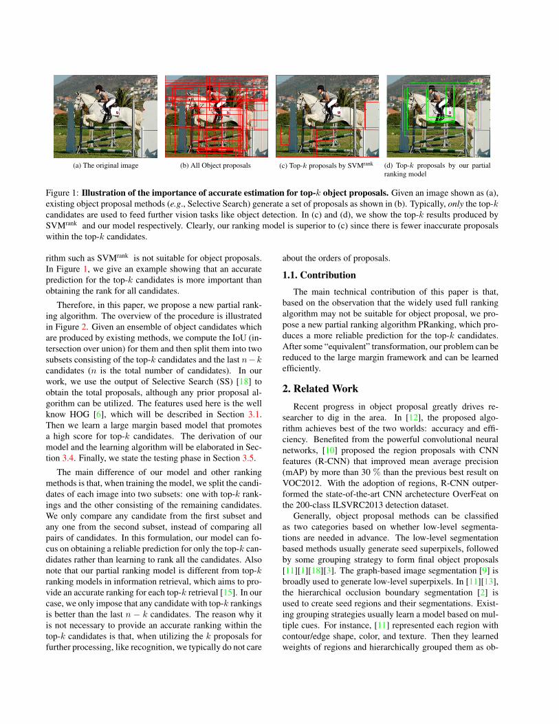
(a) The original image (b) All Object proposals (c) Top-k proposals by SVMrank (d) Top-k proposals by our partialranking model

Figure 1: Illustration of the importance of accurate estimation for top-k object proposals. Given an image shown as (a),existing object proposal methods (e.g., Selective Search) generate a set of proposals as shown in (b). Typically, only the top-kcandidates are used to feed further vision tasks like object detection. In (c) and (d), we show the top-k results produced bySVMrank and our model respectively. Clearly, our ranking model is superior to (c) since there is fewer inaccurate proposalswithin the top-k candidates.

rithm such as SVMrank is not suitable for object proposals.In Figure 1, we give an example showing that an accurateprediction for the top-k candidates is more important thanobtaining the rank for all candidates.

Therefore, in this paper, we propose a new partial rank-ing algorithm. The overview of the procedure is illustratedin Figure 2. Given an ensemble of object candidates whichare produced by existing methods, we compute the IoU (in-tersection over union) for them and then split them into twosubsets consisting of the top-k candidates and the last n−kcandidates (n is the total number of candidates). In ourwork, we use the output of Selective Search (SS) [18] toobtain the total proposals, although any prior proposal al-gorithm can be utilized. The features used here is the wellknow HOG [6], which will be described in Section 3.1.Then we learn a large margin based model that promotesa high score for top-k candidates. The derivation of ourmodel and the learning algorithm will be elaborated in Sec-tion 3.4. Finally, we state the testing phase in Section 3.5.

The main difference of our model and other rankingmethods is that, when training the model, we split the candi-dates of each image into two subsets: one with top-k rank-ings and the other consisting of the remaining candidates.We only compare any candidate from the first subset andany one from the second subset, instead of comparing allpairs of candidates. In this formulation, our model can fo-cus on obtaining a reliable prediction for only the top-k can-didates rather than learning to rank all the candidates. Alsonote that our partial ranking model is different from top-kranking models in information retrieval, which aims to pro-vide an accurate ranking for each top-k retrieval [15]. In ourcase, we only impose that any candidate with top-k rankingsis better than the last n − k candidates. The reason why itis not necessary to provide an accurate ranking within thetop-k candidates is that, when utilizing the k proposals forfurther processing, like recognition, we typically do not care

about the orders of proposals.

1.1. Contribution

The main technical contribution of this paper is that,based on the observation that the widely used full rankingalgorithm may not be suitable for object proposal, we pro-pose a new partial ranking algorithm PRanking, which pro-duces a more reliable prediction for the top-k candidates.After some “equivalent” transformation, our problem can bereduced to the large margin framework and can be learnedefficiently.

2. Related WorkRecent progress in object proposal greatly drives re-

searcher to dig in the area. In [12], the proposed algo-rithm achieves best of the two worlds: accuracy and effi-ciency. Benefited from the powerful convolutional neuralnetworks, [10] proposed the region proposals with CNNfeatures (R-CNN) that improved mean average precision(mAP) by more than 30 % than the previous best result onVOC2012. With the adoption of regions, R-CNN outper-formed the state-of-the-art CNN archetecture OverFeat onthe 200-class ILSVRC2013 detection dataset.

Generally, object proposal methods can be classifiedas two categories based on whether low-level segmenta-tions are needed in advance. The low-level segmentationbased methods usually generate seed superpixels, followedby some grouping strategy to form final object proposals[11][1][18][3]. The graph-based image segmentation [9] isbroadly used to generate low-level superpixels. In [11][13],the hierarchical occlusion boundary segmentation [2] isused to create seed regions and their segmentations. Exist-ing grouping strategies usually learn a model based on mul-tiple cues. For instance, [11] represented each region withcontour/edge shape, color, and texture. Then they learnedweights of regions and hierarchically grouped them as ob-

ject candidates. [1] presented a generic objectness measurecomposed of saliency, edge density, superpixels straddlingand so on. The measures are combined in a Bayesian frame-work to qualify how likely a window covers an object. Se-lective Search [18] exhaustively merged adjacent superpix-els based on the complementary similarity measurementsincluding colour, texture, size and so forth. Endres et al.learned cascades features to rank candidates based on edgedistributions near region boundaries [7]. Rahu et al. pro-vided new objectness features and combined hypothesis bylearning a ridge regression model [17]. Manen et al. em-ployed similar features with Selective Search and mergedsuperpixels based on a randomized version of Prim’s algo-rithm [14]. [16] greedily merged adjacent superpixels byglobal and local searches with SIFT and RGB descriptors.The RIGOR method generated a pool of overlapping seg-mentations and proposed a piecewise-linear regression treefor grouping [13]. The MCG method proposed a multi-scalehierarchical segmentation and grouped multiscale regionsby features of size/location, shape and contours [3].

There are only three methods which are not based onlow-level segmentations, including Constrained Pramamet-ric Min-Cuts (CPMC) [4], Binarized Normed Gradients(Bing) [5] and EdgeBoxes [21]. CPMC generated about104 overlapping segmentations per image by solving min-cut problems and merged regions by their mid-level cuessuch as graph partition, region and gestalt properties. Binglearned an object model by cascaded SVMs in multiplescales. It speeded up the model learning by proposing anovel binarized normed gradient feature,i.e., Bing. Edge-Boxes evaluated boxes with their enclosed number of con-tours in a sliding window fashion. Unlike previous methodsbased on the edge feature, Edgeboxes removed straddlingcontours which greatly improved the proposal quality.

Hosang et al. provided a careful analysis for the state-of-the-art object proposal methods [12]. According to [12],Bing is the fastest so far. EdgeBoxes obtains the best re-call but needs to tune the parameters at each desired overlapthreshold. Selective Search obtains relatively fast speed andhigh recall. It is also attractive as it has no parameters totune. Thus, Selective Search has been widely used in topdetection methods [19][10]. The proposal based detectionmethods, such as R-CNN, select n proposals as the searchspace. Thus, it is required to assign a high score for thoseproposals with high overlap to the groundtruth. To this end,some proposal generation methods utilized ranking algo-rithms [7][4][3]. Specifically, [7][20] ranked regions usingstructured learning based on various visual cues. CPMC [4]trained a Random Forest to regress the object overlap withthe groundtruth. MCG [3] adopted the similar ranking al-gorithm as CPMC and used Maximum Marginal Relevancemeasures to diversify the ranking. All the re-ranking meth-ods mentioned above aimed to provide an accurate full rank

for all candidates. However, it is difficult and not neces-sary to learn the difference between proposals with similarIoU. For example, the difference between boxes with sim-ilar IoU, like 0.8 or 0.81, is not easy to characterize. Thismotivates us to learn a partial ranking model in this paper.

3. Problem SetupIn this paper, we focus on a new re-ranking method for

object proposal. Assume that for each image, we havean ensemble of candidates (i.e., bounding boxes) B =(b1, · · · , bn)1. Each ensemble of candidates is associatedwith a vector y = (y1, · · · , yn), with each yi being theIoU to the groundtruth of the candidate bi. Denote the inputspace as

X = {X | X = (x1, · · · ,xn)}, (1)

where xi is some feature descriptor for bi, and the outputspace as

Y = {y | y = (y1, · · · , yn)}. (2)

We are interested in learning the prediction function

f : X → Y. (3)

To be more detailed, we assume that

yi = w · xi,∀ i = 1, · · ·n, (4)

where w is the weight vector we aim to learn and “·” de-notes the inner product. In this way, the mapping functionf is formulated as follows:

f(X) = (w · xi, · · · ,w · xn). (5)

In the following, we will elaborate the design of the fea-ture descriptor and the learning algorithm for the weightvector w.

3.1. Feature

The discipline of a successful proposal algorithm is theefficiency. Thus we handcraft some simple features forcomputational efficiency. Given a bounding box b, itsfeature descriptor used here is the well known HOG fea-tures [6]. One may extract more effective features, such asthose produced by convolutional neural networks (CNNs),whose performance was carefully studied in [10]. How-ever, in this paper we focus on the ranking model ratherthan choosing the most effective features.

3.2. Partial Ranking Model

Given a training set {(Xj ,yj)}Nj=1 where N denotes thenumber of training images, we aim to learn the weight vec-tor w, such that the top-k candidates in each Xj is bet-ter than the others. Assume without loss of generality that

1For simplicity, we assume that each image has a number of n propos-als.

1. Object proposals

Positive

Negative Large Margin based model

3. Training samples 4. Feature representation

5. Train a model

2. Training sample candidates

top k

last n-k

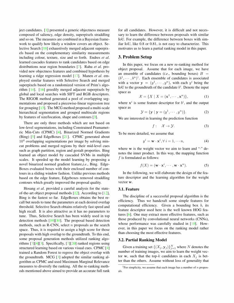
Figure 2: Overview of the learning procedure. Our system (1) takes an input image, (2) gets proposals which are producedby Selective Search, (3) split the set of candidates into the top-k subset and the last n− k subset according to the IoU to thegroundtruth, (4) computes features for each proposal, and then (5) learns a model by large-margin based model.

yj = (y1j , · · · , ynj ) is in a descending order. Thus, we actu-ally solve the following convex optimization problem:

minw

1

2‖w‖22

s.t. w · xpj ≥ w · xqj , ∀j ∈ [N ], p ∈ [k], q ∈ [n]\[k],(6)

where [N ] denotes the integer set of {1, · · · , N}.

3.3. Comparison with SVMrank

In previous work, a commonly utilized ranking model isSVMrank, which is formulated as follows:

minw

1

2‖w‖22

s.t. w · xpj ≥ w · xqj , ∀j ∈ [N ], p, q ∈ [n], p ≤ q.(7)

Note that in the formulation (6), we divide the set [n] intotwo subsets: [k] and [n]\[k]. The constraints are only im-posed between the two subsets: any candidate xpj with thetop-k ranks enjoys a higher confidence than those with thelast n−k ranks. This formulation is motivated by the practi-cal usage of object proposals: basically, proposals alleviatethe drawback of the sliding window scheme by reducing thesearch space from the whole image (over each position andscale) to a manageable number of regions (i.e., boundingboxes). After that, one may extract finer visual cues on onlythe proposals for accurate recognition and detection. Thus,essentially a good prediction for the top-k candidates is suf-ficient for a successful proposal algorithm. From this pointof view, it is more reasonable to compare the top-k candi-dates (which are of interest for the user) to the remaining

n−k ones, rather than comparing any pair from the ensem-ble of the candidates (which is the formulation of (7)).

Moreover, note that in our formulation (6), there is nocomparison between candidates within [k] nor those within[n]\[k], since when we post-process the k proposals for fur-ther recognition, we actually consider little for their ordersproduced by the ranking model.

As a matter of fact, one may have noticed that the con-straints in Problem (6) is a subset of those in Problem (7).That is, our formulation is a reasonable relaxation for theclassical SVMrank model. Besides the superiority we men-tioned above, it can be expected that the learning procedureof our problem can be more efficient than SVMrank, sincein our model, the number of constraints is reduced from12n(n− 1) to k(n− k).

At last, as we only constrain candidates belonging to dif-ferent subsets, we can transform our problem into the wellknown large margin based framework, stated as follows.

3.4. Learning

3.4.1 Large Margin Model

In practical problems, the data can be corrupted and the hardconstraints in Eq. (6) will be violated. Thus for the robust-ness of the model, it is necessary to derive a soft formula-tion. To this end, we first transform Eq. (6) to the hard largemargin based model:

minw

1

2‖w‖22

s.t. w · xpj ≥ +1,∀ p ∈ [k]

w · xqj ≤ −1,∀ q ∈ [n]\[k].

(8)

top k last n-k

(a) Formulation (6)

top k last n-k

-1

+1

(b) Formulation (8)

Figure 3: Illustration for different formulations.

The above formulation is “equivalent” to Problem (6) in thesense that the confidence of the top-k candidates producedby the model is higher than that of the last n−k candidates.In other words, the reformulation keeps the relative rank forthe subsets [k] and [n]\[k].

By introducing non-negative slack variables ξj , we ob-tain the soft margin formulation:

minw,ξ

1

2‖w‖22 + C

N∑j=1

ξj

s.t. w · xpj ≥ +1− ξj ,∀ p ∈ [k]

w · xqj ≤ −1 + ξj ,∀ q ∈ [n]\[k],

(9)

where C is a trade-off parameter. We set it as 1 for a softmargin.

3.4.2 Connection to Binary SVM

At a first sight, our soft margin formulation is similar tobinary SVM. We remark here some difference. First, forbinary SVM, the positive and negative samples are usuallypicked by some binary evaluation metric. For example, forimage classification, a sample is considered to be positive ifit contains some object. There is no ranking information inbinary SVM. In our case, we actually rank the samples andselect the top-k candidates as positive.

Also, the derivation of ours is different from binarySVM. We actually derive (9) from Eq. (6). Note that whenwe transform Eq. (6) to Eq. (8), we impose the top-k can-didates with confidence greater than 1 and the others lessthan −1. However, a more flexible way is to allow the con-fidence of the top-k candidates to be greater than some pos-itive variable δj , and the others less than −δj . In this way,we have the adaptive soft margin problem:

minw,ξ,δ

1

2‖w‖22 + C

N∑j=1

ξj

s.t. w · xpj ≥ +δj − ξj ,∀ p ∈ [k]

w · xqj ≤ −δj + ξj ,∀ q ∈ [n]\[k].

(10)

This adaptive model is of interest and we leave it for futurework.

3.5. Testing

During the testing phase, we first obtain the total n can-didates by running SS on the test sample. Then we extractthe HOG feature for each bounding box, whose confidencecan be subsequently computed by Eq. (5). After a sortingstep, we have an estimation for the top-k candidates.

4. Experiments4.1. The Dataset and Metrics

We evaluate our method on the challenging PASCAL Vi-sual Object Challenge (VOC) 2007 dataset [8]. VOC2007dataset contains 9,963 images in 20 classes and is dividedinto “train”, “val”, and “test” subsets. We conduct our ex-periments on the “train” and “test” splits. The employedevaluation metrics are Detection Rate (DR) and Mean Av-eratge Best Overlap (MABO) defined in [18]. The DR met-ric is derived from the Pascal Overlap Criterion and widelyused to evaluate the quality of proposals [1][12]. It consid-ers an object covered when the overlap (IoU) between itsground truth region and at least one proposal is larger thana threshold δ. The Average Best Overlap (ABO) calculatesthe best overlap between each ground truth region and pro-posals for each class. The MABO is the mean ABO over allclasses.

4.2. Experiment Setting

We set n = 1000 in our experiments, i.e., there are 1000candidates for re-ranking. We vary the threshold δ amongthree values 0.5, 0.7 and 0.9.

We get proposals from Selective Search (SS). That is, inthe training stage, we obtain 1000 boxes per image fromSelective Search on VOC2007 training set. k is set to be20. In case of memory bottleneck, we use the last min{n−k, 2k} candidates rather than the last n−k ones. We extractthe HOG feature [6] for all regions, each of which is resized

to 50 by 60. The cell size of HOG is 8. In the testing stage,we get 1000 proposals in sequence from Selective Searchon VOC2007 testing set. Then, we extract HOG features ofboxes and utilize our model to re-rank them.

4.3. Experiment Results

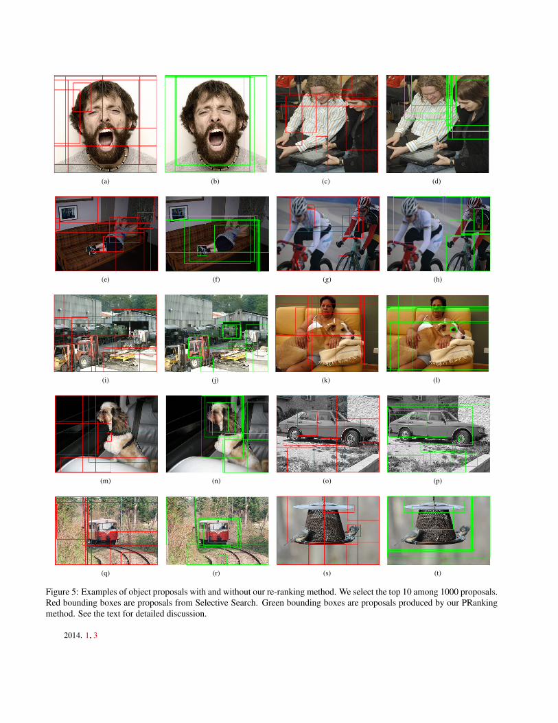
We show some exemplar results in Figure 5, where for abetter view, only the top-10 proposals are drawn on the im-age. Images with red bounding boxes are those produced bySS and results of PRanking are denoted by green boundingboxes. We can see that our method provide a more accurateestimation for the top-10 proposals. Moreover, SelectiveSearch tends to produce diverse boxes in various locations,but our top proposals are near the groundtruth. For instance,in Figure 5.(c), SS covers a pen, torso of people, while oursall contain heads which are more accurate proposals for de-tection. In Figure 5.(n), ours mainly covers the head of thedog, while no boxes from SS contain it. Our re-rankingmodel could not only select boxes covering parts of the ob-ject but also selects large boxes, such as in Figure 5.(p).

Then we report the DR produced by SS and our PRank-ing model under different threshold δ in Figure 4. Note thatwe train the model with top-20 candidates but we draw theDR curve for all top candidates. We see that our PRankingmodel generalizes really well for other top-k DR.

Specifically, as shown in Table 1 with IoU = 0.5, thedetection rate of Selective Search is less than 80.00 percentfor top-200 proposals, but PRanking reaches 84.25 percent.Our PRanking obtains an average 3.54% percent increasein detection rate compared with original proposals. Whenwe vary the δ to 0.7, i.e., a stricter evaluation metric, ourmethod achieves more improvement. As shown in Table2, the detection rate of PRanking is over 7 percent higherthan Selective Search for top-100 and top-500 proposals. Toachieve the detection rate of 78 percent, Selective Search re-quires about 1000 proposals, but our PRanking only needsabout half the number of proposals. Table 3 shows the de-tection rates with IoU of 0.9. The first proposal of SelectiveSearch is better, but our method achieves much higher de-tection rates with the increase of the number of proposals.Specifically, our PRanking reaches DR of 30.65 percent fortop-200 proposals, when Selective Search is only 22.95 per-cent. When the number of proposals reaches 1000, PRrank-ing obtains the detection rate of 45.78 when that of SelectiveSearch is still less than 40 percent.

Table 4 reports the MABO scores. The first proposal ofSelective Search is with slightly higher IoU. As the numberof proposals increases, the MABO score keeps steadily ris-ing, and our PRaning enjoys a considerable improvement inquality (about 0.0365 increase). For instance, our MABOscore reaches 0.8059 with 500 proposals, while SelectiveSearch is 0.7935.

In summary, although the proposals of Selective Search

100

101

102

103

0

20

40

60

80

100

Number of proposals

Det

ectio

n R

ate

SS−0.5PRanking−0.5SS−0.7PRanking−0.7SS−0.9PRanking−0.9

Figure 4: Detection rates w.r.t. Number of object proposals.SS-0.5, SS-0.7, and SS-0.9 represent Selective Search underIoU of 0.5, 0.7 and 0.9. Similar name usage are taken forPRanking.

are already with high quality, our model obtains a greatincrease in both detection rates and MABO scores. Thisdemonstrates that our idea of partial ranking is reasonable.We could accurately learn the margin between boundingboxes with higher IoU and low IoU. Thus, the boundingboxes with high IoU will be put in high rank by our model.

5. ConclusionIn this paper, based on the observation that it is typically

not necessary to derive a full ranking for the total candi-dates, we propose a new partial ranking model for objectproposal. The main difference of our model and other fullranking models, such as SVMrank, is that we only constrainthe relative orders of the two subsets: the top-k candidatesand the last n − k candidates. We then show that such amodel can be equivalently transformed into the large marginbased framework, in the sense of keeping the relative ranksof the two subsets. In the experiments, we show that afterthe partial re-ranking step, the detection rate of proposalsproduced by our algorithm enjoy a dramatic improvement.

References[1] B. Alexe, T. Deselaers, and V. Ferrari. What is an object? In

CVPR, pages 73–80. IEEE, 2010. 1, 2, 3, 5[2] P. Arbelaez, M. Maire, C. Fowlkes, and J. Malik. From con-

tours to regions: An empirical evaluation. In CVPR, pages2294–2301. IEEE, 2009. 2

[3] P. Arbelaez, J. Pont-Tuset, J. T. Barron, F. Marques, andJ. Malik. Multiscale combinatorial grouping. In CVPR,pages 328–335, 2014. 1, 2, 3

[4] J. Carreira and C. Sminchisescu. Constrained parametricmin-cuts for automatic object segmentation. In CVPR, pages3241–3248. IEEE, 2010. 1, 3

Table 1: Detection rate (%) w.r.t. the number of proposals for IoU threshold of 0.5. Row 1 (SS) shows Selective Searchperformance. Row 2 (SS+PRanking) shows results after applying our method on the proposals of SS.

Algorithms 1 10 50 100 200 500 800 1000SS 13.75 37.44 62.34 71.48 79.86 88.16 91.50 92.87

SS+PRanking 14.98 41.71 66.51 76.09 84.25 91.96 94.25 94.87

Table 2: Detection rate (%) w.r.t. the number of proposals for IoU threshold of 0.7. Row 1 (SS) shows Selective Searchperformance. Row 2 (SS+PRanking) shows results after applying our method on the proposals of SS.

Algorithms 1 10 50 100 200 500 800 1000SS 5.99 17.25 38.54 48.28 58.22 70.08 75.72 78.26

SS+PRanking 6.68 22.69 44.81 55.28 65.91 78.03 82.17 83.19

Table 3: Detection rate (%) w.r.t. the number of proposals for IoU threshold of 0.9. Row 1 (SS) shows Selective Searchperformance. Row 2 (SS+PRanking) shows results after applying our method on the proposals of SS.

Algorithms 1 10 50 100 200 500 800 1000SS 1.21 3.93 11.31 16.93 22.95 31.78 36.55 38.66

SS+PRanking 0.78 5.64 15.96 22.59 30.65 40.98 44.81 45.78

Table 4: Mean Average Best Overlap (MABO) w.r.t. the number of proposals. Row 1 (SS) shows the MABO scores ofSelective Search. Row 2 (SS+PRanking) shows MABO scores after applying our re-ranking method on Selective Search.

Algorithms 1 10 50 100 200 500 800 1000SS 0.1990 0.4082 0.5739 0.6393 0.6986 0.7646 0.7935 0.8062

SS+PRanking 0.1909 0.4249 0.6018 0.6718 0.7380 0.8059 0.8288 0.8342

[5] M.-M. Cheng, Z. Zhang, W.-Y. Lin, and P. Torr. Bing: Bina-rized normed gradients for objectness estimation at 300fps.In CVPR, pages 3286–3293, 2014. 1, 3

[6] N. Dalal and B. Triggs. Histograms of oriented gradients forhuman detection. In CVPR, volume 1, pages 886–893. IEEE,2005. 2, 3, 5

[7] I. Endres and D. Hoiem. Category independent object pro-posals. In ECCV, pages 575–588. Springer, 2010. 1, 3

[8] M. Everingham, L. Van Gool, C. K. Williams, J. Winn, andA. Zisserman. The pascal visual object classes (voc) chal-lenge. International journal of computer vision, 88(2):303–338, 2010. 5

[9] P. F. Felzenszwalb and D. P. Huttenlocher. Efficient graph-based image segmentation. International Journal of Com-puter Vision, 59(2):167–181, 2004. 2

[10] R. Girshick, J. Donahue, T. Darrell, and J. Malik. Rich fea-ture hierarchies for accurate object detection and semanticsegmentation. In CVPR, pages 580–587, 2014. 2, 3

[11] C. Gu, J. J. Lim, P. Arbelaez, and J. Malik. Recognitionusing regions. In CVPR, pages 1030–1037. IEEE, 2009. 2

[12] J. Hosang, R. Benenson, and B. Schiele. How good are de-tection proposals, really? arXiv preprint arXiv:1406.6962,2014. 2, 3, 5

[13] A. Humayun, F. Li, and J. M. Rehg. Rigor: Reusing in-ference in graph cuts for generating object regions. pages336–343, 2014. 2, 3

[14] S. Manen, M. Guillaumin, and L. V. Gool. Prime objectproposals with randomized prim’s algorithm. In ICCV, pages2536–2543. IEEE, 2013. 3

[15] S. Niu, J. Guo, Y. Lan, and X. Cheng. Top-k learning torank: labeling, ranking and evaluation. In Proceedings of the35th international ACM SIGIR conference on Research anddevelopment in information retrieval, pages 751–760. ACM,2012. 2

[16] R. P. and K. J. . R. E. Generating object segmentation pro-posals using global and local search. In CVPR, pages 2417–2424, 2014. 3

[17] E. Rahtu, J. Kannala, and M. Blaschko. Learning a categoryindependent object detection cascade. In ICCV, pages 1052–1059. IEEE, 2011. 3

[18] J. R. Uijlings, K. E. van de Sande, T. Gevers, and A. W.Smeulders. Selective search for object recognition. Interna-tional journal of computer vision, 104(2):154–171, 2013. 1,2, 3, 5

[19] X. Wang, M. Yang, S. Zhu, and Y. Lin. Regionlets for genericobject detection. In Computer Vision (ICCV), 2013 IEEEInternational Conference on, pages 17–24. IEEE, 2013. 3

[20] P. Yadollahpour, D. Batra, and G. Shakhnarovich. Discrimi-native re-ranking of diverse segmentations. In CVPR, pages1923–1930. IEEE, 2013. 3

[21] C. L. Zitnick and P. Dollar. Edge boxes: Locating objectproposals from edges. In ECCV, pages 391–405. Springer,

(a) (b) (c) (d)

(e) (f) (g) (h)

(i) (j) (k) (l)

(m) (n) (o) (p)

(q) (r) (s) (t)

Figure 5: Examples of object proposals with and without our re-ranking method. We select the top 10 among 1000 proposals.Red bounding boxes are proposals from Selective Search. Green bounding boxes are proposals produced by our PRankingmethod. See the text for detailed discussion.

2014. 1, 3