Embed Size (px)
Citation preview

NWChem User Documentation
Release 5.1.1
Molecular Sciences Software GroupW.R. Wiley Environmental Molecular Sciences Laboratory
Pacific Northwest National LaboratoryP.O. Box 999, Richland, WA 99352
August 2008

2

DISCLAIMER
This material was prepared as an account of work sponsored by an agency of the United States Government. Neitherthe United States Government nor the United States Department of Energy, nor Battelle, nor any of their employees,MAKES ANY WARRANTY, EXPRESS OR IMPLIED, OR ASSUMES ANY LEGAL LIABILITY OR RESPON-SIBILITY FOR THE ACCURACY, COMPLETENESS, OR USEFULNESS OF ANY INFORMATION, APPARA-TUS, PRODUCT, SOFTWARE, OR PROCESS DISCLOSED, OR REPRESENTS THAT ITS USE WOULD NOTINFRINGE PRIVATELY OWNED RIGHTS.
LIMITED USE
This software (including any documentation) is being made available to you for your internal use only, solely foruse in performance of work directly for the U.S. Federal Government or work under contracts with the U.S. Departmentof Energy or other U.S. Federal Government agencies. This software is a version which has not yet been evaluated andcleared for commercialization. Adherence to this notice may be necessary for the author, Battelle Memorial Institute,to successfully assert copyright in and commercialize this software. This software is not intended for duplication ordistribution to third parties without the permission of the Manager of Software Products at Pacific Northwest NationalLaboratory, Richland, Washington, 99352.
ACKNOWLEDGMENT
This software and its documentation were produced with Government support under Contract Number DE-AC05-76RL01830 awarded by the United States Department of Energy. The Government retains a paid-up non-exclusive,irrevocable worldwide license to reproduce, prepare derivative works, perform publicly and display publicly by or forthe Government, including the right to distribute to other Government contractors.
3

4
AUTHOR DISCLAIMER
This software contains proprietary information of the authors, Pacific Northwest National Laboratory (PNNL),and the US Department of Energy (USDOE). The information herein shall not be disclosed to others, and shall not bereproduced whole or in part, without written permission from PNNL or USDOE. The information contained in thisdocument is provided “AS IS” without guarantee of accuracy. Use of this software is prohibited without written per-mission from PNNL or USDOE. The authors, PNNL, and USDOE make no representations or warranties whatsoeverwith respect to this software, including the implied warranty of merchant-ability or fitness for a particular purpose.The user assumes all risks, including consequential loss or damage, in respect to the use of the software. In addition,PNNL and the authors shall not be obligated to correct or maintain the program, or notify the user community ofmodifications or updates that will be made over the course of time.
Contents
1 Introduction 21
1.1 Citation . . . . . . . . . . . . . . . . . . . . . . . . . . . . . . . . . . . . . . . . . . . . . . . . . . 21
1.2 User Feedback . . . . . . . . . . . . . . . . . . . . . . . . . . . . . . . . . . . . . . . . . . . . . . 22
2 Getting Started 25
2.1 Input File Structure . . . . . . . . . . . . . . . . . . . . . . . . . . . . . . . . . . . . . . . . . . . . 25
2.2 Simple Input File — SCF geometry optimization . . . . . . . . . . . . . . . . . . . . . . . . . . . . 26
2.3 Water Molecule Sample Input File . . . . . . . . . . . . . . . . . . . . . . . . . . . . . . . . . . . . 27
2.4 Input Format and Syntax for Directives . . . . . . . . . . . . . . . . . . . . . . . . . . . . . . . . . . 29
2.4.1 Input Format . . . . . . . . . . . . . . . . . . . . . . . . . . . . . . . . . . . . . . . . . . . 29
2.4.2 Format and syntax of directives . . . . . . . . . . . . . . . . . . . . . . . . . . . . . . . . . 30
3 NWChem Architecture 33
3.1 Database Structure . . . . . . . . . . . . . . . . . . . . . . . . . . . . . . . . . . . . . . . . . . . . 33
3.2 Persistence of data and restart . . . . . . . . . . . . . . . . . . . . . . . . . . . . . . . . . . . . . . . 35
4 Functionality 37
4.1 Molecular electronic structure . . . . . . . . . . . . . . . . . . . . . . . . . . . . . . . . . . . . . . 37
4.2 Relativistic effects . . . . . . . . . . . . . . . . . . . . . . . . . . . . . . . . . . . . . . . . . . . . . 39
4.3 Pseudopotential plane-wave electronic structure . . . . . . . . . . . . . . . . . . . . . . . . . . . . . 39
4.4 Molecular dynamics . . . . . . . . . . . . . . . . . . . . . . . . . . . . . . . . . . . . . . . . . . . . 40
4.5 Python . . . . . . . . . . . . . . . . . . . . . . . . . . . . . . . . . . . . . . . . . . . . . . . . . . . 40
4.6 Parallel tools and libraries (ParSoft) . . . . . . . . . . . . . . . . . . . . . . . . . . . . . . . . . . . 41
5 Top-level directives 43
5.1 START and RESTART — Start-up mode . . . . . . . . . . . . . . . . . . . . . . . . . . . . . . . . . 43
5.2 SCRATCH_DIR and PERMANENT_DIR — File directories . . . . . . . . . . . . . . . . . . . . . . . 45
5

6 CONTENTS
5.3 MEMORY — Control of memory limits . . . . . . . . . . . . . . . . . . . . . . . . . . . . . . . . . . 46
5.4 ECHO — Print input file . . . . . . . . . . . . . . . . . . . . . . . . . . . . . . . . . . . . . . . . . . 47
5.5 TITLE — Specify job title . . . . . . . . . . . . . . . . . . . . . . . . . . . . . . . . . . . . . . . . 48
5.6 PRINT and NOPRINT — Print control . . . . . . . . . . . . . . . . . . . . . . . . . . . . . . . . . . 48
5.7 SET — Enter data in the RTDB . . . . . . . . . . . . . . . . . . . . . . . . . . . . . . . . . . . . . 49
5.8 UNSET — Delete data in the RTDB . . . . . . . . . . . . . . . . . . . . . . . . . . . . . . . . . . . 51
5.9 STOP — Terminate processing . . . . . . . . . . . . . . . . . . . . . . . . . . . . . . . . . . . . . . 51
5.10 TASK — Perform a task . . . . . . . . . . . . . . . . . . . . . . . . . . . . . . . . . . . . . . . . . 51
5.10.1 TASK Directive for Electronic Structure Calculations . . . . . . . . . . . . . . . . . . . . . . 52
5.10.2 TASK Directive for Special Operations . . . . . . . . . . . . . . . . . . . . . . . . . . . . . 53
5.10.3 TASK Directive for the Bourne Shell . . . . . . . . . . . . . . . . . . . . . . . . . . . . . . . 54
5.10.4 TASK Directive for QM/MM simulations . . . . . . . . . . . . . . . . . . . . . . . . . . . . 55
5.10.5 TASK Directive for BSSE calculations . . . . . . . . . . . . . . . . . . . . . . . . . . . . . . 55
5.11 CHARGE — Total system charge . . . . . . . . . . . . . . . . . . . . . . . . . . . . . . . . . . . . . 57
5.12 ECCE_PRINT — Print information for Ecce . . . . . . . . . . . . . . . . . . . . . . . . . . . . . . 58
6 Geometries 59
6.1 Keywords on the GEOMETRY directive . . . . . . . . . . . . . . . . . . . . . . . . . . . . . . . . . . 60
6.2 SYMMETRY — Symmetry Group Input . . . . . . . . . . . . . . . . . . . . . . . . . . . . . . . . . . 62
6.3 Cartesian coordinate input . . . . . . . . . . . . . . . . . . . . . . . . . . . . . . . . . . . . . . . . 63
6.4 ZMATRIX — Z-matrix input . . . . . . . . . . . . . . . . . . . . . . . . . . . . . . . . . . . . . . . 64
6.5 ZCOORD — Forcing internal coordinates . . . . . . . . . . . . . . . . . . . . . . . . . . . . . . . . . 70
6.6 Applying constraints in geometry optimizations . . . . . . . . . . . . . . . . . . . . . . . . . . . . . 71
6.7 SYSTEM — Lattice parameters for periodic systems . . . . . . . . . . . . . . . . . . . . . . . . . . . 71
7 Basis sets 73
7.1 Basis set library . . . . . . . . . . . . . . . . . . . . . . . . . . . . . . . . . . . . . . . . . . . . . . 75
7.2 Explicit basis set definition . . . . . . . . . . . . . . . . . . . . . . . . . . . . . . . . . . . . . . . . 76
7.3 Combinations of library and explicit basis set input . . . . . . . . . . . . . . . . . . . . . . . . . . . 77
8 Effective Core Potentials 79
8.1 Scalar ECPs . . . . . . . . . . . . . . . . . . . . . . . . . . . . . . . . . . . . . . . . . . . . . . . . 80
8.2 Spin-orbit ECPs . . . . . . . . . . . . . . . . . . . . . . . . . . . . . . . . . . . . . . . . . . . . . . 82
9 Relativistic All-electron Approximations 85
9.1 Douglas-Kroll approximation . . . . . . . . . . . . . . . . . . . . . . . . . . . . . . . . . . . . . . . 86

CONTENTS 7
9.2 Zeroth Order regular approximation (ZORA) . . . . . . . . . . . . . . . . . . . . . . . . . . . . . . 87
9.3 Dyall’s Modified Dirac Hamitonian approximation . . . . . . . . . . . . . . . . . . . . . . . . . . . 87
10 Hartree-Fock or Self-consistent Field 91
10.1 Wavefunction type . . . . . . . . . . . . . . . . . . . . . . . . . . . . . . . . . . . . . . . . . . . . 91
10.2 SYM — use of symmetry . . . . . . . . . . . . . . . . . . . . . . . . . . . . . . . . . . . . . . . . . 92
10.3 ADAPT – symmetry adaptation of MOs . . . . . . . . . . . . . . . . . . . . . . . . . . . . . . . . . 92
10.4 TOL2E — integral screening threshold . . . . . . . . . . . . . . . . . . . . . . . . . . . . . . . . . . 93
10.5 VECTORS — input/output of MO vectors . . . . . . . . . . . . . . . . . . . . . . . . . . . . . . . . 93
10.5.1 Superposition of fragment molecular orbitals . . . . . . . . . . . . . . . . . . . . . . . . . . 96
10.5.2 Atomic guess orbitals with charged atoms . . . . . . . . . . . . . . . . . . . . . . . . . . . . 101
10.6 Accuracy of initial guess . . . . . . . . . . . . . . . . . . . . . . . . . . . . . . . . . . . . . . . . . 102
10.7 THRESH — convergence threshold . . . . . . . . . . . . . . . . . . . . . . . . . . . . . . . . . . . . 102
10.8 MAXITER — iteration limit . . . . . . . . . . . . . . . . . . . . . . . . . . . . . . . . . . . . . . . . 102
10.9 PROFILE — performance profile . . . . . . . . . . . . . . . . . . . . . . . . . . . . . . . . . . . . 103
10.10DIIS — DIIS convergence . . . . . . . . . . . . . . . . . . . . . . . . . . . . . . . . . . . . . . . . 103
10.11DIRECT and SEMIDIRECT — recomputation of integrals . . . . . . . . . . . . . . . . . . . . . . . 103
10.11.1 Integral File Size and Format for the SCF Module . . . . . . . . . . . . . . . . . . . . . . . . 105
10.12SCF Convergence Control Options . . . . . . . . . . . . . . . . . . . . . . . . . . . . . . . . . . . . 106
10.13NR — controlling the Newton-Raphson . . . . . . . . . . . . . . . . . . . . . . . . . . . . . . . . . 107
10.14LEVEL — level-shifting the orbital Hessian . . . . . . . . . . . . . . . . . . . . . . . . . . . . . . . 107
10.15Orbital Localization . . . . . . . . . . . . . . . . . . . . . . . . . . . . . . . . . . . . . . . . . . . . 108
10.16Printing Information from the SCF Module . . . . . . . . . . . . . . . . . . . . . . . . . . . . . . . 110
10.17Hartree-Fock or SCF, MCSCF and MP2 Gradients . . . . . . . . . . . . . . . . . . . . . . . . . . . 111
11 DFT for Molecules (DFT) 113
11.1 Specification of Basis Sets for the DFT Module . . . . . . . . . . . . . . . . . . . . . . . . . . . . . 116
11.2 VECTORS and MAX_OVL — KS-MO Vectors . . . . . . . . . . . . . . . . . . . . . . . . . . . . . . 116
11.3 XC and DECOMP — Exchange-Correlation Potentials . . . . . . . . . . . . . . . . . . . . . . . . . . 116
11.3.1 Exchange-Correlation Functionals . . . . . . . . . . . . . . . . . . . . . . . . . . . . . . . . 118
11.3.2 Combined Exchange and Correlation Functionals . . . . . . . . . . . . . . . . . . . . . . . . 118
11.3.3 Meta-GGA Functionals . . . . . . . . . . . . . . . . . . . . . . . . . . . . . . . . . . . . . . 119
11.4 LB94 and CS00 — Asymptotic correction . . . . . . . . . . . . . . . . . . . . . . . . . . . . . . . 119
11.5 Sample input file . . . . . . . . . . . . . . . . . . . . . . . . . . . . . . . . . . . . . . . . . . . . . 120
11.6 ITERATIONS — Number of SCF iterations . . . . . . . . . . . . . . . . . . . . . . . . . . . . . . . 123

8 CONTENTS
11.7 CONVERGENCE — SCF Convergence Control . . . . . . . . . . . . . . . . . . . . . . . . . . . . . . 123
11.8 CDFT — Constrained DFT . . . . . . . . . . . . . . . . . . . . . . . . . . . . . . . . . . . . . . . . 125
11.9 SMEAR — Fractional Occupation of the Molecular Orbitals . . . . . . . . . . . . . . . . . . . . . . . 126
11.10GRID — Numerical Integration of the XC Potential . . . . . . . . . . . . . . . . . . . . . . . . . . . 127
11.10.1 Angular grids . . . . . . . . . . . . . . . . . . . . . . . . . . . . . . . . . . . . . . . . . . . 129
11.10.2 Partitioning functions . . . . . . . . . . . . . . . . . . . . . . . . . . . . . . . . . . . . . . . 131
11.10.3 Radial grids . . . . . . . . . . . . . . . . . . . . . . . . . . . . . . . . . . . . . . . . . . . . 131
11.10.4 Disk usage for Grid . . . . . . . . . . . . . . . . . . . . . . . . . . . . . . . . . . . . . . . . 131
11.11TOLERANCES — Screening tolerances . . . . . . . . . . . . . . . . . . . . . . . . . . . . . . . . . 131
11.12DIRECT, SEMIDIRECT and NOIO — Hardware Resource Control . . . . . . . . . . . . . . . . . . 132
11.13ODFT and MULT — Open shell systems . . . . . . . . . . . . . . . . . . . . . . . . . . . . . . . . . 133
11.14SIC — Self-Interaction Correction . . . . . . . . . . . . . . . . . . . . . . . . . . . . . . . . . . . . 133
11.15MULLIKEN — Mulliken analysis . . . . . . . . . . . . . . . . . . . . . . . . . . . . . . . . . . . . . 134
11.16BSSE — Basis Set Superposition Error . . . . . . . . . . . . . . . . . . . . . . . . . . . . . . . . . 134
11.17DISP — Empirical Long-range Contribution (vdW) . . . . . . . . . . . . . . . . . . . . . . . . . . 134
11.18Print Control . . . . . . . . . . . . . . . . . . . . . . . . . . . . . . . . . . . . . . . . . . . . . . . 135
12 Spin-Orbit DFT (SODFT) 137
13 COSMO 141
14 CIS, TDHF, and TDDFT 145
14.1 Overview . . . . . . . . . . . . . . . . . . . . . . . . . . . . . . . . . . . . . . . . . . . . . . . . . 145
14.2 Performance of CIS, TDHF, and TDDFT methods . . . . . . . . . . . . . . . . . . . . . . . . . . . . 146
14.3 Input syntax . . . . . . . . . . . . . . . . . . . . . . . . . . . . . . . . . . . . . . . . . . . . . . . . 147
14.4 Keywords of TDDFT input block . . . . . . . . . . . . . . . . . . . . . . . . . . . . . . . . . . . . . 148
14.4.1 CIS and RPA — the Tamm–Dancoff approximation . . . . . . . . . . . . . . . . . . . . . . 148
14.4.2 NROOTS — the number of excited states . . . . . . . . . . . . . . . . . . . . . . . . . . . . 148
14.4.3 MAXVECS — the subspace size . . . . . . . . . . . . . . . . . . . . . . . . . . . . . . . . . 148
14.4.4 SINGLET and NOSINGLET — singlet excited states . . . . . . . . . . . . . . . . . . . . . . 148
14.4.5 TRIPLET and NOTRIPLET — triplet excited states . . . . . . . . . . . . . . . . . . . . . . 149
14.4.6 THRESH — the convergence threshold of Davidson iteration . . . . . . . . . . . . . . . . . . 149
14.4.7 MAXITER — the maximum number of Davidson iteration . . . . . . . . . . . . . . . . . . . 149
14.4.8 TARGET and TARGETSYM— the target root and its symmetry . . . . . . . . . . . . . . . . . 149
14.4.9 SYMMETRY — restricting the excited state symmetry . . . . . . . . . . . . . . . . . . . . . . 149

CONTENTS 9
14.4.10 ALGORITHM — algorithms for tensor contractions . . . . . . . . . . . . . . . . . . . . . . . 149
14.4.11 FREEZE — the frozen core/virtual approximation . . . . . . . . . . . . . . . . . . . . . . . 150
14.4.12 PRINT — the verbosity . . . . . . . . . . . . . . . . . . . . . . . . . . . . . . . . . . . . . 150
14.5 Sample input . . . . . . . . . . . . . . . . . . . . . . . . . . . . . . . . . . . . . . . . . . . . . . . 150
15 Tensor Contraction Engine Module: CI, MBPT, and CC 155
15.1 Overview . . . . . . . . . . . . . . . . . . . . . . . . . . . . . . . . . . . . . . . . . . . . . . . . . 155
15.2 Performance of CI, MBPT, and CC methods . . . . . . . . . . . . . . . . . . . . . . . . . . . . . . . 157
15.3 Algorithms of CI, MBPT, and CC methods . . . . . . . . . . . . . . . . . . . . . . . . . . . . . . . 158
15.3.1 Spin, spatial, and index permutation symmetry . . . . . . . . . . . . . . . . . . . . . . . . . 158
15.3.2 Runtime orbital range tiling . . . . . . . . . . . . . . . . . . . . . . . . . . . . . . . . . . . 158
15.3.3 Dynamic load balancing parallelism . . . . . . . . . . . . . . . . . . . . . . . . . . . . . . . 158
15.3.4 Parallel I/O schemes . . . . . . . . . . . . . . . . . . . . . . . . . . . . . . . . . . . . . . . 158
15.4 Input syntax . . . . . . . . . . . . . . . . . . . . . . . . . . . . . . . . . . . . . . . . . . . . . . . . 159
15.5 Keywords of TCE input block . . . . . . . . . . . . . . . . . . . . . . . . . . . . . . . . . . . . . . 160
15.5.1 HF, SCF, or DFT — the reference wave function . . . . . . . . . . . . . . . . . . . . . . . . 160
15.5.2 CCSD,CCSDT,CCSDTQ,CISD,CISDT,CISDTQ, MBPT2,MBPT3,MBPT4, etc. — the correla-tion models . . . . . . . . . . . . . . . . . . . . . . . . . . . . . . . . . . . . . . . . . . . . 161
15.5.3 THRESH — the convergence threshold of iterative solutions of amplitude equations . . . . . . 163
15.5.4 MAXITER — the maximum number of iterations . . . . . . . . . . . . . . . . . . . . . . . . 163
15.5.5 IO — parallel I/O scheme . . . . . . . . . . . . . . . . . . . . . . . . . . . . . . . . . . . . 163
15.5.6 DIIS — the convergence acceleration . . . . . . . . . . . . . . . . . . . . . . . . . . . . . . 164
15.5.7 FREEZE — the frozen core/virtual approximation . . . . . . . . . . . . . . . . . . . . . . . 164
15.5.8 NROOTS — the number of excited states . . . . . . . . . . . . . . . . . . . . . . . . . . . . 165
15.5.9 TARGET and TARGETSYM — the target root and its symmetry . . . . . . . . . . . . . . . . . 165
15.5.10 SYMMETRY — restricting the excited state symmetry . . . . . . . . . . . . . . . . . . . . . . 165
15.5.11 2EORB — alternative storage of two-electron integrals . . . . . . . . . . . . . . . . . . . . . 165
15.5.12 2EMET — alternative storage of two-electron integrals . . . . . . . . . . . . . . . . . . . . . 166
15.5.13 DIPOLE — the ground- and excited-state dipole moments . . . . . . . . . . . . . . . . . . . 167
15.5.14 (NO)FOCK — (not) recompute Fock matrix . . . . . . . . . . . . . . . . . . . . . . . . . . 167
15.5.15 PRINT — the verbosity . . . . . . . . . . . . . . . . . . . . . . . . . . . . . . . . . . . . . 167
15.6 Sample input . . . . . . . . . . . . . . . . . . . . . . . . . . . . . . . . . . . . . . . . . . . . . . . 167
15.7 TCE gradients . . . . . . . . . . . . . . . . . . . . . . . . . . . . . . . . . . . . . . . . . . . . . . . 174
15.8 TCE Response Properties . . . . . . . . . . . . . . . . . . . . . . . . . . . . . . . . . . . . . . . . . 175
15.8.1 Introduction . . . . . . . . . . . . . . . . . . . . . . . . . . . . . . . . . . . . . . . . . . . . 175

10 CONTENTS
15.8.2 Performance . . . . . . . . . . . . . . . . . . . . . . . . . . . . . . . . . . . . . . . . . . . 175
15.8.3 Input . . . . . . . . . . . . . . . . . . . . . . . . . . . . . . . . . . . . . . . . . . . . . . . 175
15.8.4 Examples . . . . . . . . . . . . . . . . . . . . . . . . . . . . . . . . . . . . . . . . . . . . . 176
15.9 TCE Restart Capability . . . . . . . . . . . . . . . . . . . . . . . . . . . . . . . . . . . . . . . . . . 177
15.9.1 Overview . . . . . . . . . . . . . . . . . . . . . . . . . . . . . . . . . . . . . . . . . . . . . 177
15.9.2 Input . . . . . . . . . . . . . . . . . . . . . . . . . . . . . . . . . . . . . . . . . . . . . . . 178
15.9.3 Examples . . . . . . . . . . . . . . . . . . . . . . . . . . . . . . . . . . . . . . . . . . . . . 178
15.10Maximizing performance . . . . . . . . . . . . . . . . . . . . . . . . . . . . . . . . . . . . . . . . . 179
15.10.1 Memory considerations and IO schemes . . . . . . . . . . . . . . . . . . . . . . . . . . . . . 179
15.10.2 Processor count . . . . . . . . . . . . . . . . . . . . . . . . . . . . . . . . . . . . . . . . . . 179
15.10.3 SCF options . . . . . . . . . . . . . . . . . . . . . . . . . . . . . . . . . . . . . . . . . . . . 179
15.10.4 Convergence criteria . . . . . . . . . . . . . . . . . . . . . . . . . . . . . . . . . . . . . . . 179
15.10.5 Integral storage, transformation algorithms and tilesizes . . . . . . . . . . . . . . . . . . . . 179
16 MP2 181
16.1 FREEZE — Freezing orbitals . . . . . . . . . . . . . . . . . . . . . . . . . . . . . . . . . . . . . . . 182
16.2 TIGHT — Increased precision . . . . . . . . . . . . . . . . . . . . . . . . . . . . . . . . . . . . . . 183
16.3 SCRATCHDISK — Limiting I/O usage . . . . . . . . . . . . . . . . . . . . . . . . . . . . . . . . . 183
16.4 PRINT and NOPRINT . . . . . . . . . . . . . . . . . . . . . . . . . . . . . . . . . . . . . . . . . . 183
16.5 VECTORS — MO vectors . . . . . . . . . . . . . . . . . . . . . . . . . . . . . . . . . . . . . . . . . 183
16.6 RI-MP2 fitting basis . . . . . . . . . . . . . . . . . . . . . . . . . . . . . . . . . . . . . . . . . . . . 184
16.7 FILE3C — RI-MP2 3-center integral filename . . . . . . . . . . . . . . . . . . . . . . . . . . . . . 185
16.8 RIAPPROX — RI-MP2 Approximation . . . . . . . . . . . . . . . . . . . . . . . . . . . . . . . . . 185
16.9 Advanced options for RI-MP2 . . . . . . . . . . . . . . . . . . . . . . . . . . . . . . . . . . . . . . 185
16.9.1 Control of linear dependence . . . . . . . . . . . . . . . . . . . . . . . . . . . . . . . . . . . 185
16.9.2 Reference Spin Mapping for RI-MP2 Calculations . . . . . . . . . . . . . . . . . . . . . . . 185
16.9.3 Batch Sizes for the RI-MP2 Calculation . . . . . . . . . . . . . . . . . . . . . . . . . . . . . 186
16.9.4 Energy Memory Allocation Mode: RI-MP2 Calculation . . . . . . . . . . . . . . . . . . . . 187
16.9.5 Local Memory Usage in Three-Center Transformation . . . . . . . . . . . . . . . . . . . . . 187
16.10One-electron properties and natural orbitals . . . . . . . . . . . . . . . . . . . . . . . . . . . . . . . 187
17 Multiconfiguration SCF 189
17.1 ACTIVE — Number of active orbitals . . . . . . . . . . . . . . . . . . . . . . . . . . . . . . . . . . 189
17.2 ACTELEC — Number of active electrons . . . . . . . . . . . . . . . . . . . . . . . . . . . . . . . . 190
17.3 MULTIPLICITY . . . . . . . . . . . . . . . . . . . . . . . . . . . . . . . . . . . . . . . . . . . . . 190
CONTENTS 11
17.4 SYMMETRY — Spatial symmetry of the wavefunction . . . . . . . . . . . . . . . . . . . . . . . . . . 190
17.5 STATE — Symmetry and multiplicity . . . . . . . . . . . . . . . . . . . . . . . . . . . . . . . . . . 190
17.6 VECTORS — Input/output of MO vectors . . . . . . . . . . . . . . . . . . . . . . . . . . . . . . . . 191
17.7 HESSIAN — Select preconditioner . . . . . . . . . . . . . . . . . . . . . . . . . . . . . . . . . . . 191
17.8 LEVEL — Level shift for convergence . . . . . . . . . . . . . . . . . . . . . . . . . . . . . . . . . . 191
17.9 PRINT and NOPRINT . . . . . . . . . . . . . . . . . . . . . . . . . . . . . . . . . . . . . . . . . . 191
18 Selected CI 193
18.1 Background . . . . . . . . . . . . . . . . . . . . . . . . . . . . . . . . . . . . . . . . . . . . . . . . 193
18.2 Files . . . . . . . . . . . . . . . . . . . . . . . . . . . . . . . . . . . . . . . . . . . . . . . . . . . . 194
18.3 Configuration Generation . . . . . . . . . . . . . . . . . . . . . . . . . . . . . . . . . . . . . . . . . 195
18.3.1 Specifying the reference occupation . . . . . . . . . . . . . . . . . . . . . . . . . . . . . . . 195
18.3.2 Applying creation-annihilation operators . . . . . . . . . . . . . . . . . . . . . . . . . . . . 196
18.3.3 Uniform excitation level . . . . . . . . . . . . . . . . . . . . . . . . . . . . . . . . . . . . . 197
18.4 Number of roots . . . . . . . . . . . . . . . . . . . . . . . . . . . . . . . . . . . . . . . . . . . . . . 197
18.5 Accuracy of diagonalization . . . . . . . . . . . . . . . . . . . . . . . . . . . . . . . . . . . . . . . 197
18.6 Selection thresholds . . . . . . . . . . . . . . . . . . . . . . . . . . . . . . . . . . . . . . . . . . . . 198
18.7 Mode . . . . . . . . . . . . . . . . . . . . . . . . . . . . . . . . . . . . . . . . . . . . . . . . . . . 198
18.8 Memory requirements . . . . . . . . . . . . . . . . . . . . . . . . . . . . . . . . . . . . . . . . . . . 198
18.9 Forcing regeneration of the MO integrals . . . . . . . . . . . . . . . . . . . . . . . . . . . . . . . . . 198
18.10Disabling update of the configuration list . . . . . . . . . . . . . . . . . . . . . . . . . . . . . . . . . 198
18.11Orbital locking in CI geometry optimization . . . . . . . . . . . . . . . . . . . . . . . . . . . . . . . 199
19 Coupled Cluster Calculations 201
19.1 MAXITER — Maximum number of iterations . . . . . . . . . . . . . . . . . . . . . . . . . . . . . . 201
19.2 THRESH — Convergence threshold . . . . . . . . . . . . . . . . . . . . . . . . . . . . . . . . . . . 202
19.3 TOL2E — integral screening threshold . . . . . . . . . . . . . . . . . . . . . . . . . . . . . . . . . . 202
19.4 DIISBAS — DIIS subspace dimension . . . . . . . . . . . . . . . . . . . . . . . . . . . . . . . . . 202
19.5 NODISK — disable integral caching . . . . . . . . . . . . . . . . . . . . . . . . . . . . . . . . . . . 202
19.6 FREEZE — Freezing orbitals . . . . . . . . . . . . . . . . . . . . . . . . . . . . . . . . . . . . . . . 202
19.7 IPRT — Debug printing . . . . . . . . . . . . . . . . . . . . . . . . . . . . . . . . . . . . . . . . . 203
19.8 PRINT and NOPRINT . . . . . . . . . . . . . . . . . . . . . . . . . . . . . . . . . . . . . . . . . . 203
19.9 NODISK . . . . . . . . . . . . . . . . . . . . . . . . . . . . . . . . . . . . . . . . . . . . . . . . . 203
19.10Methods (Tasks) Recognized . . . . . . . . . . . . . . . . . . . . . . . . . . . . . . . . . . . . . . . 203
19.11Debugging and Development Aids . . . . . . . . . . . . . . . . . . . . . . . . . . . . . . . . . . . . 204

12 CONTENTS
19.11.1 Switching On and Off Terms . . . . . . . . . . . . . . . . . . . . . . . . . . . . . . . . . . . 204
20 Geometry Optimization with DRIVER 205
20.1 Convergence criteria . . . . . . . . . . . . . . . . . . . . . . . . . . . . . . . . . . . . . . . . . . . 206
20.2 Available precision . . . . . . . . . . . . . . . . . . . . . . . . . . . . . . . . . . . . . . . . . . . . 206
20.3 Controlling the step length . . . . . . . . . . . . . . . . . . . . . . . . . . . . . . . . . . . . . . . . 207
20.4 Maximum number of steps . . . . . . . . . . . . . . . . . . . . . . . . . . . . . . . . . . . . . . . . 207
20.5 Discard restart information . . . . . . . . . . . . . . . . . . . . . . . . . . . . . . . . . . . . . . . . 207
20.6 Regenerate internal coordinates . . . . . . . . . . . . . . . . . . . . . . . . . . . . . . . . . . . . . . 207
20.7 Initial Hessian . . . . . . . . . . . . . . . . . . . . . . . . . . . . . . . . . . . . . . . . . . . . . . . 207
20.8 Mode or variable to follow to saddle point . . . . . . . . . . . . . . . . . . . . . . . . . . . . . . . . 208
20.9 Optimization history as XYZ files . . . . . . . . . . . . . . . . . . . . . . . . . . . . . . . . . . . . 208
20.10Print options . . . . . . . . . . . . . . . . . . . . . . . . . . . . . . . . . . . . . . . . . . . . . . . . 209
21 Geometry Optimization with STEPPER 211
21.1 MIN and TS — Minimum or transition state search . . . . . . . . . . . . . . . . . . . . . . . . . . . 211
21.2 TRACK — Mode selection . . . . . . . . . . . . . . . . . . . . . . . . . . . . . . . . . . . . . . . . 212
21.3 MAXITER — Maximum number of steps . . . . . . . . . . . . . . . . . . . . . . . . . . . . . . . . 212
21.4 TRUST — Trust radius . . . . . . . . . . . . . . . . . . . . . . . . . . . . . . . . . . . . . . . . . . 212
21.5 CONVGGM, CONVGG and CONVGE — Convergence criteria . . . . . . . . . . . . . . . . . . . . . . . 212
21.6 Backstepping in STEPPER . . . . . . . . . . . . . . . . . . . . . . . . . . . . . . . . . . . . . . . . 213
21.7 Initial Nuclear Hessian Options . . . . . . . . . . . . . . . . . . . . . . . . . . . . . . . . . . . . . . 213
22 Geometry Optimization with TROPT 215
22.1 Convergence criteria . . . . . . . . . . . . . . . . . . . . . . . . . . . . . . . . . . . . . . . . . . . 216
22.2 Available precision . . . . . . . . . . . . . . . . . . . . . . . . . . . . . . . . . . . . . . . . . . . . 217
22.3 Controlling the step length . . . . . . . . . . . . . . . . . . . . . . . . . . . . . . . . . . . . . . . . 217
22.4 Backstepping in TROPT . . . . . . . . . . . . . . . . . . . . . . . . . . . . . . . . . . . . . . . . . 217
22.5 Maximum number of steps . . . . . . . . . . . . . . . . . . . . . . . . . . . . . . . . . . . . . . . . 217
22.6 Discard restart information . . . . . . . . . . . . . . . . . . . . . . . . . . . . . . . . . . . . . . . . 217
22.7 Regenerate internal coordinates . . . . . . . . . . . . . . . . . . . . . . . . . . . . . . . . . . . . . . 217
22.8 Initial Hessian . . . . . . . . . . . . . . . . . . . . . . . . . . . . . . . . . . . . . . . . . . . . . . . 218
22.9 Mode or variable to follow to saddle point . . . . . . . . . . . . . . . . . . . . . . . . . . . . . . . . 218
22.10Optimization history as XYZ file . . . . . . . . . . . . . . . . . . . . . . . . . . . . . . . . . . . . . 219
22.11Print options . . . . . . . . . . . . . . . . . . . . . . . . . . . . . . . . . . . . . . . . . . . . . . . . 219

CONTENTS 13
23 Minimum Energy Path with MEPGS 221
23.1 Convergence criteria . . . . . . . . . . . . . . . . . . . . . . . . . . . . . . . . . . . . . . . . . . . 221
23.2 Available precision . . . . . . . . . . . . . . . . . . . . . . . . . . . . . . . . . . . . . . . . . . . . 222
23.3 Controlling the step length . . . . . . . . . . . . . . . . . . . . . . . . . . . . . . . . . . . . . . . . 222
23.4 Moving away from the saddle point . . . . . . . . . . . . . . . . . . . . . . . . . . . . . . . . . . . 222
23.5 Maximum number of MEPGS steps . . . . . . . . . . . . . . . . . . . . . . . . . . . . . . . . . . . 222
23.6 Maximum number of steps . . . . . . . . . . . . . . . . . . . . . . . . . . . . . . . . . . . . . . . . 222
23.7 Initial Hessian . . . . . . . . . . . . . . . . . . . . . . . . . . . . . . . . . . . . . . . . . . . . . . . 223
23.8 Selecting the side to traverse . . . . . . . . . . . . . . . . . . . . . . . . . . . . . . . . . . . . . . . 223
23.9 Using mass . . . . . . . . . . . . . . . . . . . . . . . . . . . . . . . . . . . . . . . . . . . . . . . . 223
23.10Minimum energy path saved XYZ file . . . . . . . . . . . . . . . . . . . . . . . . . . . . . . . . . . 223
23.11MEPGS usage . . . . . . . . . . . . . . . . . . . . . . . . . . . . . . . . . . . . . . . . . . . . . . . 223
24 Constraints for Geometry Optimization 225
25 Hybrid Calculations with ONIOM 227
25.1 Real, model and intermediate geometries . . . . . . . . . . . . . . . . . . . . . . . . . . . . . . . . . 228
25.1.1 Link atoms . . . . . . . . . . . . . . . . . . . . . . . . . . . . . . . . . . . . . . . . . . . . 229
25.1.2 Numbering of the link atoms . . . . . . . . . . . . . . . . . . . . . . . . . . . . . . . . . . . 230
25.2 High, medium and low theories . . . . . . . . . . . . . . . . . . . . . . . . . . . . . . . . . . . . . . 230
25.2.1 Basis specification . . . . . . . . . . . . . . . . . . . . . . . . . . . . . . . . . . . . . . . . 230
25.2.2 Effective core potentials . . . . . . . . . . . . . . . . . . . . . . . . . . . . . . . . . . . . . 230
25.2.3 General input strings . . . . . . . . . . . . . . . . . . . . . . . . . . . . . . . . . . . . . . . 230
25.3 Use of symmetry . . . . . . . . . . . . . . . . . . . . . . . . . . . . . . . . . . . . . . . . . . . . . 231
25.4 Molecular orbital files . . . . . . . . . . . . . . . . . . . . . . . . . . . . . . . . . . . . . . . . . . . 231
25.5 Restarting . . . . . . . . . . . . . . . . . . . . . . . . . . . . . . . . . . . . . . . . . . . . . . . . . 232
25.6 Examples . . . . . . . . . . . . . . . . . . . . . . . . . . . . . . . . . . . . . . . . . . . . . . . . . 232
25.6.1 Hydrocarbon bond energy . . . . . . . . . . . . . . . . . . . . . . . . . . . . . . . . . . . . 232
25.6.2 Optimization and frequencies . . . . . . . . . . . . . . . . . . . . . . . . . . . . . . . . . . 233
25.6.3 A three-layer example . . . . . . . . . . . . . . . . . . . . . . . . . . . . . . . . . . . . . . 235
25.6.4 DFT with and without charge fitting . . . . . . . . . . . . . . . . . . . . . . . . . . . . . . . 236
26 Hessians 239
26.1 Hessian Module Input . . . . . . . . . . . . . . . . . . . . . . . . . . . . . . . . . . . . . . . . . . . 239
26.1.1 Defining the wavefunction threshold . . . . . . . . . . . . . . . . . . . . . . . . . . . . . . . 239

14 CONTENTS
26.1.2 Profile . . . . . . . . . . . . . . . . . . . . . . . . . . . . . . . . . . . . . . . . . . . . . . . 240
26.1.3 Print Control . . . . . . . . . . . . . . . . . . . . . . . . . . . . . . . . . . . . . . . . . . . 240
27 Vibrational frequencies 241
27.1 Vibrational Module Input . . . . . . . . . . . . . . . . . . . . . . . . . . . . . . . . . . . . . . . . . 241
27.1.1 Hessian File Reuse . . . . . . . . . . . . . . . . . . . . . . . . . . . . . . . . . . . . . . . . 242
27.1.2 Redefining Masses of Elements . . . . . . . . . . . . . . . . . . . . . . . . . . . . . . . . . 242
27.1.3 Temp or Temperature . . . . . . . . . . . . . . . . . . . . . . . . . . . . . . . . . . . . . . . 243
27.1.4 Animation . . . . . . . . . . . . . . . . . . . . . . . . . . . . . . . . . . . . . . . . . . . . 243
27.1.5 An Example Input Deck . . . . . . . . . . . . . . . . . . . . . . . . . . . . . . . . . . . . . 244
28 DPLOT 245
28.1 GAUSSIAN — Gaussian Cube format . . . . . . . . . . . . . . . . . . . . . . . . . . . . . . . . . . 245
28.2 TITLE — Title directive . . . . . . . . . . . . . . . . . . . . . . . . . . . . . . . . . . . . . . . . . 245
28.3 LIMITXYZ — Plot limits . . . . . . . . . . . . . . . . . . . . . . . . . . . . . . . . . . . . . . . . . 245
28.4 SPIN — Density to be plotted . . . . . . . . . . . . . . . . . . . . . . . . . . . . . . . . . . . . . . 246
28.5 OUTPUT — Filename . . . . . . . . . . . . . . . . . . . . . . . . . . . . . . . . . . . . . . . . . . . 246
28.6 VECTORS — MO vector file name . . . . . . . . . . . . . . . . . . . . . . . . . . . . . . . . . . . . 246
28.7 DENSMAT — Density matrix file name . . . . . . . . . . . . . . . . . . . . . . . . . . . . . . . . . . 246
28.8 WHERE — Density evaluation . . . . . . . . . . . . . . . . . . . . . . . . . . . . . . . . . . . . . . 246
28.9 ORBITAL — Orbital sub-space . . . . . . . . . . . . . . . . . . . . . . . . . . . . . . . . . . . . . 247
28.10Examples . . . . . . . . . . . . . . . . . . . . . . . . . . . . . . . . . . . . . . . . . . . . . . . . . 247
29 Electron Transfer Calculations with ET 249
29.1 VECTORS — input of MO vectors for ET reactant and product states . . . . . . . . . . . . . . . . . . 250
29.2 FOCK/NOFOCK — method for calculating the two-electron contribution to VRP . . . . . . . . . . . . 250
29.3 TOL2E — integral screening threshold . . . . . . . . . . . . . . . . . . . . . . . . . . . . . . . . . . 250
29.4 Example . . . . . . . . . . . . . . . . . . . . . . . . . . . . . . . . . . . . . . . . . . . . . . . . . 250
30 Properties 253
30.1 Property keywords . . . . . . . . . . . . . . . . . . . . . . . . . . . . . . . . . . . . . . . . . . . . 254
30.1.1 Nbofile . . . . . . . . . . . . . . . . . . . . . . . . . . . . . . . . . . . . . . . . . . . . . . 254
31 VSCF 255
32 Pseudopotential plane-wave density functional theory (NWPW) 257
32.1 PSPW Tasks . . . . . . . . . . . . . . . . . . . . . . . . . . . . . . . . . . . . . . . . . . . . . . . . 258

CONTENTS 15
32.1.1 Simulation Cell . . . . . . . . . . . . . . . . . . . . . . . . . . . . . . . . . . . . . . . . . . 261
32.1.2 Unit Cell Optimization . . . . . . . . . . . . . . . . . . . . . . . . . . . . . . . . . 263
32.1.3 DPLOT . . . . . . . . . . . . . . . . . . . . . . . . . . . . . . . . . . . . . . . . . . . . . . 263
32.1.4 Wannier . . . . . . . . . . . . . . . . . . . . . . . . . . . . . . . . . . . . . . . . . . . . . 264
32.1.5 Self-Interaction Corrections . . . . . . . . . . . . . . . . . . . . . . . . . . . . 265
32.1.6 Point Charge Analysis . . . . . . . . . . . . . . . . . . . . . . . . . . . . . . . . . 266
32.1.7 Car-Parrinello . . . . . . . . . . . . . . . . . . . . . . . . . . . . . . . . . . . . . . . 266
32.1.8 Adding Geometry Constraints To A Car-Parrinello Simulation . . . . 269
32.1.9 QM/MM . . . . . . . . . . . . . . . . . . . . . . . . . . . . . . . . . . . . . . . . . . . . . . 270
32.1.10 PSP_GENERATOR . . . . . . . . . . . . . . . . . . . . . . . . . . . . . . . . . . . . . . . . 272
32.1.11 WAVEFUNCTION_INITIALIZER . . . . . . . . . . . . . . . . . . . . . . . . . . . . . . . 274
32.1.12 V_WAVEFUNCTION_INITIALIZER . . . . . . . . . . . . . . . . . . . . . . . . . . . . . 276
32.1.13 WAVEFUNCTION_EXPANDER . . . . . . . . . . . . . . . . . . . . . . . . . . . . . . . . . 277
32.1.14 STEEPEST_DESCENT . . . . . . . . . . . . . . . . . . . . . . . . . . . . . . . . . . . . . 278
32.2 Band Tasks . . . . . . . . . . . . . . . . . . . . . . . . . . . . . . . . . . . . . . . . . . . . . . . . 280
32.2.1 Brillouin Zone . . . . . . . . . . . . . . . . . . . . . . . . . . . . . . . . . . . . . . . . . . 282
32.2.2 BAND_DPLOT . . . . . . . . . . . . . . . . . . . . . . . . . . . . . . . . . . . . . . . . . . 282
32.2.3 SMEAR - Fractional Occupation of the Molecular Orbitals . . . . . . . . . . . . . . . . . . . 284
32.3 PAW Tasks . . . . . . . . . . . . . . . . . . . . . . . . . . . . . . . . . . . . . . . . . . . . . . . . 284
32.4 Pseudopotential and PAW basis Libraries . . . . . . . . . . . . . . . . . . . . . . . . . . . . . . . . 286
32.5 NWPW RTDB Entries and DataFiles . . . . . . . . . . . . . . . . . . . . . . . . . . . . . . . . . . . 288
32.5.1 Ion Positions . . . . . . . . . . . . . . . . . . . . . . . . . . . . . . . . . . . . . . . . . . . 289
32.5.2 Ion Velocities . . . . . . . . . . . . . . . . . . . . . . . . . . . . . . . . . . . . . . . . . . . 289
32.5.3 Wavefunction Datafile . . . . . . . . . . . . . . . . . . . . . . . . . . . . . . . . . . . . . . 289
32.5.4 Velocity Wavefunction Datafile . . . . . . . . . . . . . . . . . . . . . . . . . . . . . . . . . 289
32.5.5 Formatted Pseudopotential Datafile . . . . . . . . . . . . . . . . . . . . . . . . . . . . . . . 289
32.5.6 One-Dimensional Pseudopotential Datafile . . . . . . . . . . . . . . . . . . . . . . . . . . . 289
32.5.7 PSPW Car-Parrinello Output Datafiles . . . . . . . . . . . . . . . . . . . . . . . . . . . . . . 290
32.6 Car-Parrinello Scheme for Ab Initio Molecular Dynamics . . . . . . . . . . . . . . . . . . . . . . . . 291
32.6.1 Verlet Algorithm for Integration . . . . . . . . . . . . . . . . . . . . . . . . . . . . . . . . . 292
32.6.2 Constant Temperature Simulations: Nose-Hoover Thermostats . . . . . . . . . . . . . . . . . 293
32.7 PSPW Tutorial 1: Minimizing the geometry for a C2 molecule . . . . . . . . . . . . . . . . . . . . . 294
32.8 PSPW Tutorial 2: Running a Car-Parrinello Simulation . . . . . . . . . . . . . . . . . . . . . . . . . 295
32.9 PSPW Tutorial 3: optimizing a unit cell and geometry for Silicon-Carbide . . . . . . . . . . . . . . . 295
16 CONTENTS
32.10PSPW Tutorial 4: QM/MM simulation for CCl4 + 64H2O . . . . . . . . . . . . . . . . . . . . . . . . 296
32.11Band Tutorial 1: Minimizing the energy of a silicon-carbide crystal by running a PSPW and Bandsimulation in tandem . . . . . . . . . . . . . . . . . . . . . . . . . . . . . . . . . . . . . . . . . . . 300
32.12BAND Tutorial 2: optimizing a unit cell and geometry for Silicon-Carbide . . . . . . . . . . . . . . . 301
32.13BAND Tutorial 3: optimizing a unit cell and geometry for Aluminum with fractional occupation . . . 302
32.14PAW Tutorial . . . . . . . . . . . . . . . . . . . . . . . . . . . . . . . . . . . . . . . . . . . . . . . 303
32.15PAW Tutorial 2: optimizing a unit cell and geometry for Silicon-Carbide . . . . . . . . . . . . . . . . 304
32.16PAW Tutorial 2: Running a Car-Parrinello Simulation . . . . . . . . . . . . . . . . . . . . . . . . . . 305
32.17NWPW Capabilities and Limitations . . . . . . . . . . . . . . . . . . . . . . . . . . . . . . . . . . . 305
32.18Questions and Difficulties . . . . . . . . . . . . . . . . . . . . . . . . . . . . . . . . . . . . . . . . . 306
33 Electrostatic potentials 307
33.1 Grid specification . . . . . . . . . . . . . . . . . . . . . . . . . . . . . . . . . . . . . . . . . . . . . 307
33.2 Constraints . . . . . . . . . . . . . . . . . . . . . . . . . . . . . . . . . . . . . . . . . . . . . . . . 308
33.3 Restraints . . . . . . . . . . . . . . . . . . . . . . . . . . . . . . . . . . . . . . . . . . . . . . . . . 309
34 Prepare 311
34.1 Default database directories . . . . . . . . . . . . . . . . . . . . . . . . . . . . . . . . . . . . . . . . 313
34.2 System name and coordinate source . . . . . . . . . . . . . . . . . . . . . . . . . . . . . . . . . . . 314
34.3 Sequence file generation . . . . . . . . . . . . . . . . . . . . . . . . . . . . . . . . . . . . . . . . . 315
34.4 Topology file generation . . . . . . . . . . . . . . . . . . . . . . . . . . . . . . . . . . . . . . . . . 316
34.5 Appending to an existing topology file . . . . . . . . . . . . . . . . . . . . . . . . . . . . . . . . . . 318
34.6 Generating a restart file . . . . . . . . . . . . . . . . . . . . . . . . . . . . . . . . . . . . . . . . . . 319
35 Molecular dynamics 323
35.1 Introduction . . . . . . . . . . . . . . . . . . . . . . . . . . . . . . . . . . . . . . . . . . . . . . . . 323
35.1.1 Spacial decomposition . . . . . . . . . . . . . . . . . . . . . . . . . . . . . . . . . . . . . . 323
35.1.2 Topology . . . . . . . . . . . . . . . . . . . . . . . . . . . . . . . . . . . . . . . . . . . . . 324
35.1.3 Files . . . . . . . . . . . . . . . . . . . . . . . . . . . . . . . . . . . . . . . . . . . . . . . . 324
35.1.4 Databases . . . . . . . . . . . . . . . . . . . . . . . . . . . . . . . . . . . . . . . . . . . . . 325
35.1.5 Force fields . . . . . . . . . . . . . . . . . . . . . . . . . . . . . . . . . . . . . . . . . . . . 326
35.2 Format of fragment files . . . . . . . . . . . . . . . . . . . . . . . . . . . . . . . . . . . . . . . . . 326
35.3 Creating segment files . . . . . . . . . . . . . . . . . . . . . . . . . . . . . . . . . . . . . . . . . . . 326
35.4 Creating sequence files . . . . . . . . . . . . . . . . . . . . . . . . . . . . . . . . . . . . . . . . . . 326
35.5 Creating topology files . . . . . . . . . . . . . . . . . . . . . . . . . . . . . . . . . . . . . . . . . . 326
35.6 Creating restart files . . . . . . . . . . . . . . . . . . . . . . . . . . . . . . . . . . . . . . . . . . . . 327

CONTENTS 17
35.7 Molecular simulations . . . . . . . . . . . . . . . . . . . . . . . . . . . . . . . . . . . . . . . . . . 327
35.8 System specification . . . . . . . . . . . . . . . . . . . . . . . . . . . . . . . . . . . . . . . . . . . 327
35.9 Restarting and continuing simulations . . . . . . . . . . . . . . . . . . . . . . . . . . . . . . . . . . 328
35.10Parameter set . . . . . . . . . . . . . . . . . . . . . . . . . . . . . . . . . . . . . . . . . . . . . . . 328
35.11Energy minimization algorithms . . . . . . . . . . . . . . . . . . . . . . . . . . . . . . . . . . . . . 328
35.12Multi-configuration thermodynamic integration . . . . . . . . . . . . . . . . . . . . . . . . . . . . . 329
35.13Time and integration algorithm directives . . . . . . . . . . . . . . . . . . . . . . . . . . . . . . . . 330
35.14Ensemble selection . . . . . . . . . . . . . . . . . . . . . . . . . . . . . . . . . . . . . . . . . . . . 330
35.15Velocity reassignments . . . . . . . . . . . . . . . . . . . . . . . . . . . . . . . . . . . . . . . . . . 331
35.16Cutoff radii . . . . . . . . . . . . . . . . . . . . . . . . . . . . . . . . . . . . . . . . . . . . . . . . 331
35.17Polarization . . . . . . . . . . . . . . . . . . . . . . . . . . . . . . . . . . . . . . . . . . . . . . . . 332
35.18External electrostatic field . . . . . . . . . . . . . . . . . . . . . . . . . . . . . . . . . . . . . . . . 332
35.19Constraints . . . . . . . . . . . . . . . . . . . . . . . . . . . . . . . . . . . . . . . . . . . . . . . . 332
35.20Long range interaction corrections . . . . . . . . . . . . . . . . . . . . . . . . . . . . . . . . . . . . 332
35.21Fixing coordinates . . . . . . . . . . . . . . . . . . . . . . . . . . . . . . . . . . . . . . . . . . . . 333
35.22Special options . . . . . . . . . . . . . . . . . . . . . . . . . . . . . . . . . . . . . . . . . . . . . . 333
35.23Autocorrelation function . . . . . . . . . . . . . . . . . . . . . . . . . . . . . . . . . . . . . . . . . 334
35.24Print options . . . . . . . . . . . . . . . . . . . . . . . . . . . . . . . . . . . . . . . . . . . . . . . . 334
35.25Periodic updates . . . . . . . . . . . . . . . . . . . . . . . . . . . . . . . . . . . . . . . . . . . . . . 335
35.26Recording . . . . . . . . . . . . . . . . . . . . . . . . . . . . . . . . . . . . . . . . . . . . . . . . . 336
35.27Program control options . . . . . . . . . . . . . . . . . . . . . . . . . . . . . . . . . . . . . . . . . 337
36 Analysis 341
36.1 System specification . . . . . . . . . . . . . . . . . . . . . . . . . . . . . . . . . . . . . . . . . . . 341
36.2 Reference coordinates . . . . . . . . . . . . . . . . . . . . . . . . . . . . . . . . . . . . . . . . . . . 341
36.3 File specification . . . . . . . . . . . . . . . . . . . . . . . . . . . . . . . . . . . . . . . . . . . . . 342
36.4 Selection . . . . . . . . . . . . . . . . . . . . . . . . . . . . . . . . . . . . . . . . . . . . . . . . . 343
36.5 Coordinate analysis . . . . . . . . . . . . . . . . . . . . . . . . . . . . . . . . . . . . . . . . . . . . 344
36.6 Essential dynamics analysis . . . . . . . . . . . . . . . . . . . . . . . . . . . . . . . . . . . . . . . . 346
36.7 Trajectory format conversion . . . . . . . . . . . . . . . . . . . . . . . . . . . . . . . . . . . . . . . 346
36.8 Electrostatic potentials . . . . . . . . . . . . . . . . . . . . . . . . . . . . . . . . . . . . . . . . . . 348
37 Combined quantum and molecular mechanics 349
37.1 Preparation of the restart and topology files . . . . . . . . . . . . . . . . . . . . . . . . . . . . . . . 349
37.2 Molecular Mechanics Parameters . . . . . . . . . . . . . . . . . . . . . . . . . . . . . . . . . . . . . 352

18 CONTENTS
37.3 Quantum Mechanical Parameters . . . . . . . . . . . . . . . . . . . . . . . . . . . . . . . . . . . . . 352
37.4 QM/MM interface parameters . . . . . . . . . . . . . . . . . . . . . . . . . . . . . . . . . . . . . . 352
38 File formats 357
38.1 Format fragment file . . . . . . . . . . . . . . . . . . . . . . . . . . . . . . . . . . . . . . . . . . . 357
38.2 Format segment file . . . . . . . . . . . . . . . . . . . . . . . . . . . . . . . . . . . . . . . . . . . . 357
38.3 Format sequence file . . . . . . . . . . . . . . . . . . . . . . . . . . . . . . . . . . . . . . . . . . . 357
38.4 Format trajectory file . . . . . . . . . . . . . . . . . . . . . . . . . . . . . . . . . . . . . . . . . . . 357
38.5 Format free energy file . . . . . . . . . . . . . . . . . . . . . . . . . . . . . . . . . . . . . . . . . . 357
38.6 Format root mean square deviation file . . . . . . . . . . . . . . . . . . . . . . . . . . . . . . . . . . 357
38.7 Format property file . . . . . . . . . . . . . . . . . . . . . . . . . . . . . . . . . . . . . . . . . . . . 357
39 Dynamical Nucleation Theory Monte Carlo 367
39.1 SubGroups . . . . . . . . . . . . . . . . . . . . . . . . . . . . . . . . . . . . . . . . . . . . . . . . 367
39.2 Input Syntax . . . . . . . . . . . . . . . . . . . . . . . . . . . . . . . . . . . . . . . . . . . . . . . . 368
39.3 Definition of Monomers . . . . . . . . . . . . . . . . . . . . . . . . . . . . . . . . . . . . . . . . . 368
39.4 DNTMC runtime options . . . . . . . . . . . . . . . . . . . . . . . . . . . . . . . . . . . . . . . . . 369
39.5 Print Control . . . . . . . . . . . . . . . . . . . . . . . . . . . . . . . . . . . . . . . . . . . . . . . 370
39.6 Selected File Formats . . . . . . . . . . . . . . . . . . . . . . . . . . . . . . . . . . . . . . . . . . . 371
39.7 DNTMC Restart . . . . . . . . . . . . . . . . . . . . . . . . . . . . . . . . . . . . . . . . . . . . . . 372
39.8 Task Directives . . . . . . . . . . . . . . . . . . . . . . . . . . . . . . . . . . . . . . . . . . . . . . 372
39.9 Example . . . . . . . . . . . . . . . . . . . . . . . . . . . . . . . . . . . . . . . . . . . . . . . . . . 373
40 Controlling NWChem with Python 375
40.1 How to input and run a Python program inside NWChem . . . . . . . . . . . . . . . . . . . . . . . . 375
40.2 NWChem extensions . . . . . . . . . . . . . . . . . . . . . . . . . . . . . . . . . . . . . . . . . . . 376
40.3 Examples . . . . . . . . . . . . . . . . . . . . . . . . . . . . . . . . . . . . . . . . . . . . . . . . . 378
40.3.1 Hello world . . . . . . . . . . . . . . . . . . . . . . . . . . . . . . . . . . . . . . . . . . . . 378
40.3.2 Scanning a basis exponent . . . . . . . . . . . . . . . . . . . . . . . . . . . . . . . . . . . . 378
40.3.3 Scanning a basis exponent revisited. . . . . . . . . . . . . . . . . . . . . . . . . . . . . . . . 379
40.3.4 Scanning a geometric variable . . . . . . . . . . . . . . . . . . . . . . . . . . . . . . . . . . 380
40.3.5 Scan using the BSSE counterpoise corrected energy . . . . . . . . . . . . . . . . . . . . . . 380
40.3.6 Scan the geometry and compute the energy and gradient . . . . . . . . . . . . . . . . . . . . 381
40.3.7 Reaction energies varying the basis set . . . . . . . . . . . . . . . . . . . . . . . . . . . . . . 382
40.3.8 Using the database . . . . . . . . . . . . . . . . . . . . . . . . . . . . . . . . . . . . . . . . 383

CONTENTS 19
40.3.9 Handling exceptions from NWChem . . . . . . . . . . . . . . . . . . . . . . . . . . . . . . . 383
40.3.10 Accessing geometry information — a temporary hack . . . . . . . . . . . . . . . . . . . . . 384
40.3.11 Scaning a basis exponent yet again — plotting and handling child processes . . . . . . . . . . 385
40.4 Troubleshooting . . . . . . . . . . . . . . . . . . . . . . . . . . . . . . . . . . . . . . . . . . . . . . 386
41 Interfaces to Other Programs 387
41.1 DIRDYVTST — DIRect Dynamics for Variational Transition State Theory . . . . . . . . . . . . . . . 387
41.1.1 Introduction . . . . . . . . . . . . . . . . . . . . . . . . . . . . . . . . . . . . . . . . . . . . 388
41.1.2 Files . . . . . . . . . . . . . . . . . . . . . . . . . . . . . . . . . . . . . . . . . . . . . . . . 388
41.1.3 Detailed description of the input . . . . . . . . . . . . . . . . . . . . . . . . . . . . . . . . . 388
42 Acknowledgments 395
A Standard Basis Sets 397
B Sample input files 413
B.1 Water SCF calculation and geometry optimization in a 6-31g basis . . . . . . . . . . . . . . . . . . . 413
B.1.1 Job 1. Single point SCF energy . . . . . . . . . . . . . . . . . . . . . . . . . . . . . . . . . 413
B.1.2 Job 2. Restarting and perform a geometry optimization . . . . . . . . . . . . . . . . . . . . . 413
B.2 Compute the polarizability of Ne using finite field . . . . . . . . . . . . . . . . . . . . . . . . . . . . 414
B.2.1 Job 1. Compute the atomic energy . . . . . . . . . . . . . . . . . . . . . . . . . . . . . . . . 414
B.2.2 Job 2. Compute the energy with applied field . . . . . . . . . . . . . . . . . . . . . . . . . . 414
B.3 SCF energy of H2CO using ECPs for C and O . . . . . . . . . . . . . . . . . . . . . . . . . . . . . . 414
B.4 MP2 optimization and CCSD(T) on nitrogen . . . . . . . . . . . . . . . . . . . . . . . . . . . . . . . 416
C Examples of geometries using symmetry 419
C.1 Cs methanol . . . . . . . . . . . . . . . . . . . . . . . . . . . . . . . . . . . . . . . . . . . . . . . . 419
C.2 C2v water . . . . . . . . . . . . . . . . . . . . . . . . . . . . . . . . . . . . . . . . . . . . . . . . . 419
C.3 D2h acetylene . . . . . . . . . . . . . . . . . . . . . . . . . . . . . . . . . . . . . . . . . . . . . . . 420
C.4 D2h ethylene . . . . . . . . . . . . . . . . . . . . . . . . . . . . . . . . . . . . . . . . . . . . . . . . 420
C.5 Td methane . . . . . . . . . . . . . . . . . . . . . . . . . . . . . . . . . . . . . . . . . . . . . . . . 420
C.6 Ih buckminsterfullerene . . . . . . . . . . . . . . . . . . . . . . . . . . . . . . . . . . . . . . . . . . 420
C.7 S4 porphyrin . . . . . . . . . . . . . . . . . . . . . . . . . . . . . . . . . . . . . . . . . . . . . . . . 421
C.8 D3h iron penta-carbonyl . . . . . . . . . . . . . . . . . . . . . . . . . . . . . . . . . . . . . . . . . . 421
C.9 D3d sodium crown ether . . . . . . . . . . . . . . . . . . . . . . . . . . . . . . . . . . . . . . . . . 422
C.10 C3v ammonia . . . . . . . . . . . . . . . . . . . . . . . . . . . . . . . . . . . . . . . . . . . . . . . 422

20 CONTENTS
C.11 D6h benzene . . . . . . . . . . . . . . . . . . . . . . . . . . . . . . . . . . . . . . . . . . . . . . . . 422
C.12 C3h BO3H3 . . . . . . . . . . . . . . . . . . . . . . . . . . . . . . . . . . . . . . . . . . . . . . . . 422
C.13 D5d ferrocene . . . . . . . . . . . . . . . . . . . . . . . . . . . . . . . . . . . . . . . . . . . . . . . 423
C.14 C4v SF5Cl . . . . . . . . . . . . . . . . . . . . . . . . . . . . . . . . . . . . . . . . . . . . . . . . . 423
C.15 C2h trans-dichloroethylene . . . . . . . . . . . . . . . . . . . . . . . . . . . . . . . . . . . . . . . . 423
C.16 D2d CH2CCH2 . . . . . . . . . . . . . . . . . . . . . . . . . . . . . . . . . . . . . . . . . . . . . . 424
C.17 D5h cyclopentadiene anion . . . . . . . . . . . . . . . . . . . . . . . . . . . . . . . . . . . . . . . . 424
C.18 D4h gold tetrachloride . . . . . . . . . . . . . . . . . . . . . . . . . . . . . . . . . . . . . . . . . . . 424
D Running NWChem 425
D.1 Sequential execution . . . . . . . . . . . . . . . . . . . . . . . . . . . . . . . . . . . . . . . . . . . 425
D.2 Parallel execution on UNIX-based parallel machines including workstation clusters using TCGMSG . 425
D.3 Parallel execution on UNIX-based parallel machines including workstation clusters using MPI . . . . 426
D.4 Parallel execution on MPPs . . . . . . . . . . . . . . . . . . . . . . . . . . . . . . . . . . . . . . . . 427
D.5 IBM SP . . . . . . . . . . . . . . . . . . . . . . . . . . . . . . . . . . . . . . . . . . . . . . . . . . 427
D.6 Cray T3E . . . . . . . . . . . . . . . . . . . . . . . . . . . . . . . . . . . . . . . . . . . . . . . . . 428
D.7 Alpha systems with Quadrics switch . . . . . . . . . . . . . . . . . . . . . . . . . . . . . . . . . . . 428
D.8 Windows 98 and NT . . . . . . . . . . . . . . . . . . . . . . . . . . . . . . . . . . . . . . . . . . . 428
D.9 Tested Platforms and O/S versions . . . . . . . . . . . . . . . . . . . . . . . . . . . . . . . . . . . . 429

Chapter 1
Introduction
NWChem is a computational chemistry package designed to run on high-performance parallel supercomputers. Codecapabilities include the calculation of molecular electronic energies and analytic gradients using Hartree-Fock self-consistent field (SCF) theory, Gaussian density function theory (DFT), and second-order perturbation theory. For allmethods, geometry optimization is available to determine energy minima and transition states. Classical moleculardynamics capabilities provide for the simulation of macromolecules and solutions, including the computation of freeenergies using a variety of force fields.
NWChem is scalable, both in its ability to treat large problems efficiently, and in its utilization of available parallelcomputing resources. The code uses the parallel programming tools TCGMSG and the Global Array (GA) librarydeveloped at PNNL for the High Performance Computing and Communication (HPCC) grand-challenge softwareprogram and the Environmental Molecular Sciences Laboratory (EMSL) Project. NWChem has been optimized toperform calculations on large molecules using large parallel computers, and it is unique in this regard.
This document is intended as an aid to chemists using the code for their own applications. Users are not expectedto have a detailed understanding of the code internals, but some familiarity with the overall structure of the code,how it handles information, and the nature of the algorithms it contains will generally be helpful. The followingsections describe the structure of the input file, and give a brief overview of the code architecture. All input directivesrecognized by the code are described in detail, with options, defaults, and recommended usages, where applicable.The appendices present additional information on the molecular geometry and basis function libraries included in thecode.
1.1 Citation
The EMSL Software Agreement stipulates that the use of NWChem will be acknowledged in any publications whichuse results obtained with NWChem. The acknowledgment should be of the form:
NWChem Version 5.1.1, as developed and distributed by Pacific Northwest National Laboratory, P. O. Box999, Richland, Washington 99352 USA, and funded by the U. S. Department of Energy, was used to obtainsome of these results.
The words “A modified version of” should be added at the beginning, if appropriate. Note: Your EMSL SoftwareAgreement contains the complete specification of the required acknowledgment.
Please use the following citation when publishing results obtained with NWChem:
21

22 CHAPTER 1. INTRODUCTION
Straatsma, T.P.; Aprà, E.; Windus, T.L.; Bylaska, E.J.; de Jong, W.; Hirata, S.; Valiev, M.; Hackler, M.;Pollack, L.; Harrison, R.; Dupuis, M.; Smith, D.M.A; Nieplocha, J.; Tipparaju V.; Krishnan, M.; Auer,A.A.; Brown, E.; Cisneros, G.; Fann, G.; Früchtl, H.; Garza, J.; Hirao, K.; Kendall, R.; Nichols, J.; Tse-mekhman, K.; Wolinski, K.; Anchell, J.; Bernholdt, D.; Borowski, P.; Clark, T.; Clerc, D.; Dachsel, H.;Deegan, M.; Dyall, K.; Elwood, D.; Glendening, E.; Gutowski, M.; Hess, A.; Jaffe, J.; Johnson, B.; Ju,J.; Kobayashi, R.; Kutteh, R.; Lin, Z.; Littlefield, R.; Long, X.; Meng, B.; Nakajima, T.; Niu, S.; Rosing,M.; Sandrone, G.; Stave, M.; Taylor, H.; Thomas, G.; van Lenthe, J.; Wong, A.; Zhang, Z.; NWChem,A Computational Chemistry Package for Parallel Computers, Version 4.6 (2004), Pacific Northwest Na-tional Laboratory, Richland, Washington 99352-0999, USA.High Performance Computational Chemistry: an Overview of NWChem a Distributed Parallel Applica-tion, Kendall, R.A.; Aprà, E.; Bernholdt, D.E.; Bylaska, E.J.; Dupuis, M.; Fann, G.I.; Harrison, R.J.; Ju,J.; Nichols, J.A.; Nieplocha, J.; Straatsma, T.P.; Windus, T.L.; Wong, A.T. Computer Phys. Comm., 2000,128, 260–283 .
If you use the DIRDYVTST portion of NWChem, please also use the additional citation:
DIRDYVTST, Yao-Yuan Chuang and Donald G. Truhlar, Department of Chemistry and Super ComputerInstitute, University of Minnesota; Ricky A. Kendall,Scalable Computing Laboratory, Ames Laboratoryand Iowa State University; Bruce C. Garrett and Theresa L. Windus, Environmental Molecular SciencesLaboratory, Pacific Northwest Laboratory.
1.2 User Feedback
This software comes without warranty or guarantee of support, but we do try to meet the needs of our user community.Please send bug reports, requests for enhancement, or other comments to
When reporting problems, please provide as much information as possible, including:
• detailed description of problem
• site name
• platform you are running on, including
– vendor name
– computer model
– operating system
– compiler
• input file
• output file
Users can also subscribe to the [email protected] electronic mailing list itself. This is intendedas a general forum through which code users can contact one another and the developers, to share experience with thecode and discuss problems. Announcements of new releases and bug fixes will also be made to this list.
To subscribe to the user list, send a message to

1.2. USER FEEDBACK 23
The body of the message must contain the line
subscribe nwchem-users
The automated list manager is capable of recognizing a number of commands, including ; “subscribe”, “unsub-scribe”, “get”, “index”, “which”, “who”, “info” and “lists”. The command “end” halts processing of commands. Itwill provide some help if the message includes the line help in the body.

24 CHAPTER 1. INTRODUCTION

Chapter 2
Getting Started
This section provides an overview of NWChem input and program architecture, and the syntax used to describe theinput. See Sections 2.2 and 2.3 for examples of NWChem input files with detailed explanation.
NWChem consists of independent modules that perform the various functions of the code. Examples of modulesinclude the input parser, SCF energy, SCF analytic gradient, DFT energy, etc.. Data is passed between modules andsaved for restart using a disk-resident database or dumpfile (see Section 3).
The input to NWChem is composed of commands, called directives, which define data (such as basis sets, ge-ometries, and filenames) and the actions to be performed on that data. Directives are processed in the order presentedin the input file, with the exception of certain start-up directives (see Section 2.1) which provide critical job controlinformation, and are processed before all other input. Most directives are specific to a particular module and definedata that is used by that module only. A few directives (see Section 5) potentially affect all modules, for instance byspecifying the total electric charge on the system.
There are two types of directives. Simple directives consist of one line of input, which may contain multiple fields.Compound directives group together multiple simple directives that are in some way related and are terminated withan END directive. See the sample inputs (Sections 2.2, 2.3) and the input syntax specification (Section 2.4).
All input is free format and case is ignored except for actual data (e.g., names/tags of centers, titles). Directivesor blocks of module-specific directives (i.e., compound directives) can appear in any order, with the exception of theTASK directive (see sections 2.1 and 5.10) which is used to invoke an NWChem module. All input for a given taskmust precede the TASK directive. This input specification rule allows the concatenation of multiple tasks in a singleNWChem input file.
To make the input as short and simple as possible, most options have default values. The user needs to supplyinput only for those items that have no defaults, or for items that must be different from the defaults for the particularapplication. In the discussion of each directive, the defaults are noted, where applicable.
The input file structure is described in the following sections, and illustrated with two examples. The input formatand syntax for directives is also described in detail.
2.1 Input File Structure
The structure of an input file reflects the internal structure of NWChem. At the beginning of a calculation, NWChemneeds to determine how much memory to use, the name of the database, whether it is a new or restarted job, whereto put scratch/permanent files, etc.. It is not necessary to put this information at the top of the input file, however.
25

26 CHAPTER 2. GETTING STARTED
NWChem will read through the entire input file looking for the start-up directives. In this first pass, all other directivesare ignored.
The start-up directives are
• START
• RESTART
• SCRATCH_DIR
• PERMANENT_DIR
• MEMORY
• ECHO
After the input file has been scanned for the start-up directives, it is rewound and read sequentially. Input isprocessed either by the top-level parser (for the directives listed in Section 5, such as TITLE, SET, . . . ) or by theparsers for specific computational modules (e.g., SCF, DFT, . . . ). Any directives that have already been processed(e.g., MEMORY) are ignored. Input is read until a TASK directive (see Section 5.10) is encountered. A TASK directiverequests that a calculation be performed and specifies the level of theory and the operation to be performed. Inputprocessing then stops and the specified task is executed. The position of the TASK directive in effect marks the end ofthe input for that task. Processing of the input resumes upon the successful completion of the task, and the results ofthat task are available to subsequent tasks in the same input file.
The name of the input file is usually provided as an argument to the execute command for NWChem. That is, theexecute command looks something like the following;
nwchem input_file
The default name for the input file is nwchem.nw. If an input file name input_file is specified withoutan extension, the code assumes .nw as a default extension, and the input filename becomes input_file.nw. Ifthe code cannot locate a file named either input_file or input_file.nw (or nwchem.nw if no file name isprovided), an error is reported and execution terminates. The following section presents two input files to illustrate thedirective syntax and input file format for NWChem applications.
2.2 Simple Input File — SCF geometry optimization
A simple example of an NWChem input file is an SCF geometry optimization of the nitrogen molecule, using aDunning cc-pvdz basis set. This input file contains the bare minimum of information the user must specify to run thistype of problem — fewer than ten lines of input, as follows:
title "Nitrogen cc-pvdz SCF geometry optimization"geometry
n 0 0 0n 0 0 1.08
endbasis
n library cc-pvdzendtask scf optimize

2.3. WATER MOLECULE SAMPLE INPUT FILE 27
Examining the input line by line, it can be seen that it contains only four directives; TITLE, GEOMETRY, BASIS,and TASK. The TITLE directive is optional, and is provided as a means for the user to more easily identify out-puts from different jobs. An initial geometry is specified in Cartesian coordinates and Angstrøms by means of theGEOMETRY directive. The Dunning cc-pvdz basis is obtained from the NWChem basis library, as specified by theBASIS directive input. The TASK directive requests an SCF geometry optimization.
The GEOMETRY directive (Section 6) defaults to Cartesian coordinates and Angstrøms (options include atomicunits and Z-matrix format; see Section 6.4). The input blocks for the BASIS and GEOMETRY directives are structuredin similar fashion, i.e., name, keyword, . . . , end (In this simple example, there are no keywords). The BASIS inputblock must contain basis set information for every atom type in the geometry with which it will be used. Refer toSections 7 and 8, and Appendix A for a description of available basis sets and a discussion of how to define new ones.
The last line of this sample input file (task scf optimize) tells the program to optimize the moleculargeometry by minimizing the SCF energy. (For a description of possible tasks and the format of the TASK directive,refer to Section 5.10.)
If the input is stored in the file n2.nw, the command to run this job on a typical UNIX workstation is as follows:
nwchem n2
NWChem output is to UNIX standard output, and error messages are sent to both standard output and standarderror.
2.3 Water Molecule Sample Input File
A more complex sample problem is the optimization of a positively charged water molecule using second-orderMøller-Plesset perturbation theory (MP2), followed by a computation of frequencies at the optimized geometry. Apreliminary SCF geometry optimization is performed using a computationally inexpensive basis set (STO-3G). Thisyields a good starting guess for the optimal geometry, and any Hessian information generated will be used in the nextoptimization step. Then the optimization is finished using MP2 and a basis set with polarization functions. The finaltask is to calculate the MP2 vibrational frequencies. The input file to accomplish these three tasks is as follows:
start h2o_freq
charge 1
geometry units angstromsO 0.0 0.0 0.0H 0.0 0.0 1.0H 0.0 1.0 0.0
end
basisH library sto-3gO library sto-3g
end
scfuhf; doubletprint low

28 CHAPTER 2. GETTING STARTED
end
title "H2O+ : STO-3G UHF geometry optimization"
task scf optimize
basisH library 6-31g**O library 6-31g**
end
title "H2O+ : 6-31g** UMP2 geometry optimization"
task mp2 optimize
mp2; print none; endscf; print none; end
title "H2O+ : 6-31g** UMP2 frequencies"
task mp2 freq
The START directive (Section 5.1) tells NWChem that this run is to be started from the beginning. This directiveneed not be at the beginning of the input file, but it is commonly placed there. Existing database or vector files are tobe ignored or overwritten. The entry h2o_freq on the START line is the prefix to be used for all files created by thecalculation. This convention allows different jobs to run in the same directory or to share the same scratch directory(see Section 5.2), as long as they use different prefix names in this field.
As in the first sample problem, the geometry is given in Cartesian coordinates. In this case, the units are specifiedas Angstrøms. (Since this is the default, explicit specification of the units is not actually necessary, however.) TheCHARGE directive defines the total charge of the system. This calculation is to be done on an ion with charge +1.
A small basis set (STO-3G) is specified for the intial geometry optimization. Next, the multiple lines of the firstSCF directive in the scf ...end block specify details about the SCF calculation to be performed. UnrestrictedHartree-Fock is chosen here (by specifying the keyword uhf), rather than the default, restricted open-shell high-spin Hartree-Fock (ROHF). This is necessary for the subsequent MP2 calculation, because only UMP2 is currentlyavailable for open-shell systems (see Section 4). For open-shell systems, the spin multiplicity has to be specified(using doublet in this case), or it defaults to singlet. The print level is set to low to avoid verbose output for thestarting basis calculations.
All input up to this point affects only the settings in the runtime database. The program takes its information fromthis database, so the sequence of directives up to the first TASK directive is irrelevant. An exchange of order of thedifferent blocks or directives would not affect the result. The TASK directive, however, must be specified after allrelevant input for a given problem. The TASK directive causes the code to perform the specified calculation using theparameters set in the preceding directives. In this case, the first task is an SCF calculation with geometry optimization,specified with the input scf and optimize. (See Section 5.10 for a list of available tasks and operations.)
After the completion of any task, settings in the database are used in subsequent tasks without change, unlessthey are overridden by new input directives. In this example, before the second task (task mp2 optimize), abetter basis set (6-31G**) is defined and the title is changed. The second TASK directive invokes an MP2 geometryoptimization.

2.4. INPUT FORMAT AND SYNTAX FOR DIRECTIVES 29
Once the MP2 optimization is completed, the geometry obtained in the calculation is used to perform a frequencycalculation. This task is invoked by the keyword freq in the final TASK directive, task mp2 freq. The secondderivatives of the energy are calculated as numerical derivatives of analytical gradients. The intermediate energiesand gradients are not of interest in this case, so output from the SCF and MP2 modules is disabled with the PRINTdirectives.
2.4 Input Format and Syntax for Directives
This section describes the input format and the syntax used in the rest of this documentation to describe the formatof directives. The input format for the directives used in NWChem is similar to that of UNIX shells, which is alsoused in other chemistry packages, most notably GAMESS-UK. An input line is parsed into whitespace (blanks ortabs) separating tokens or fields. Any token that contains whitespace must be enclosed in double quotes in order to beprocessed correctly. For example, the basis set with the descriptive name modified Dunning DZ must appear ina directive as "modified Dunning DZ", since the name consists of three separate words.
2.4.1 Input Format
A (physical) line in the input file is terminated with a newline character (also known as a ‘return’ or ‘enter’ character).A semicolon (;) can be also used to indicate the end of an input line, allowing a single physical line of input to containmultiple logical lines of input. For example, five lines of input for the GEOMETRY directive can be entered as follows;
geometryO 0 0 0H 0 1.430 1.107H 0 -1.430 1.107
end
These same five lines could be entered on a single line, as
geometry; O 0 0 0; H 0 1.430 1.107; H 0 -1.430 1.107; end
This one physical input line comprises five logical input lines. Each logical or physical input line must be no longerthan 1023 characters.
In the input file:
• a string, token, or field is a sequence of ASCII characters (NOTE: if the string includes blanks or tabs (i.e., whitespace), the entire string must be enclosed in double quotes).
• \ (backslash) at the end of a line concatenates it with the next line. Note that a space character is automaticallyinserted at this point so that it is not possible to split tokens across lines. A backslash is also used to quote specialcharacters such as whitespace, semi-colons, and hash symbols so as to avoid their special meaning (NOTE: thesespecial symbols must be quoted with the backslash even when enclosed within double quotes).
• ; (semicolon) is used to mark the end of a logical input line within a physical line of input.
• # (the hash or pound symbol) is the comment character. All characters following # (up to the end of the physicalline) are ignored.

30 CHAPTER 2. GETTING STARTED
• If any input line (excluding Python programs, Section 40) begins with the string INCLUDE (ignoring case) andis followed by a valid file name, then the data in that file are read as if they were included into the currentinput file at the current line. Up to three levels of nested include files are supported. The user should note thatinputting a basis set from the standard basis library (Section 7) uses one level of include.
• Data is read from the input file until an end-of-file is detected, or until the string EOF (ignoring case) is encoun-tered at the beginning of an input line.
2.4.2 Format and syntax of directives
Directives consist of a directive name, keywords, and optional input, and may contain one line or many. Simpledirectives consist of a single line of input with one or more fields. Compound directives can have multiple input lines,and can also include other optional simple and compound directives. A compound directive is terminated with an ENDdirective. The directives START (see Section 5.1) and ECHO (see Section 5.4) are examples of simple directives. Thedirective GEOMETRY (see Section 6) is an example of a compound directive.
Some limited checking of the input for self-consistency is performed by the input module, but most defaults areimposed by the application modules at runtime. It is therefore usually impossible to determine beforehand whether ornot all selected options are consistent with each other.
In the rest of this document, the following notation and syntax conventions are used in the generic descriptions ofthe NWChem input.
• a directive name always appears in all-capitals, and in computer typeface (e.g., GEOMETRY, BASIS, SCF). Notethat the case of directives and keywords is ignored in the actual input.
• a keyword always appears in lower case, in computer typeface (e.g., swap, print, units, bqbq).
• variable names always appear in lower case, in computer typeface, and enclosed in angle brackets to distinguishthem from keywords (e.g., <input_filename>, <basisname>, <tag>).
• $variable$ is used to indicate the substitution of the value of a variable.
• () is used to group items (the parentheses and other special symbols should not appear in the input).
• || separate exclusive options, parameters, or formats.
• [ ] enclose optional entries that have a default value.
• < > enclose a type, a name of a value to be specified, or a default value, if any.
• \ is used to concatenate lines in a description.
• ... is used to indicate indefinite continuation of a list.
An input parameter is identified in the description of the directive by prefacing the name of the item with the typeof data expected, i.e.,
• string – an ASCII character string
• integer – integer value(s) for a variable or an array
• logical – true/false logical variable
• real – real floating point value(s) for a variable or an array

2.4. INPUT FORMAT AND SYNTAX FOR DIRECTIVES 31
• double – synonymous with real
If an input item is not prefaced by one of these type names, it is assumed to be of type “string”.
In addition, integer lists may be specified using Fortran triplet notation, which interprets lo:hi:inc as lo,lo+inc, lo+2*inc, . . . , hi. For example, where a list of integers is expected in the input, the following two linesare equivalent
7 10 21:27:2 1:3 997 10 21 23 25 27 1 2 3 99
(In Fortran triplet notation, the increment, if unstated, is 1; e.g., 1:3 = 1:3:1.)
The directive VECTORS (Section 10.5) is presented here as an example of an NWChem input directive. Thegeneral form of the directive is as follows:
VECTORS [input (<string input_movecs default atomic>) || \(project <string basisname> <string filename>)] \
[swap [(alpha||beta)] <integer vec1 vec2> ...] \[output <string output_movecs default $file_prefix$.movecs>]
This directive contains three optional keywords, as indicated by the three main sets of square brackets enclosing thekeywords input, swap, and output. The keyword input allows the user to specify the source of the molecularorbital vectors. There are two mutually exclusive options for specifying the vectors, as indicated by the || symbolseparating the option descriptions;
(<string input_movecs default atomic>) || \(project <string basisname> <string filename>) \
The first option, (<string input_movecs default atomic>), allows the user to specify an ASCIIcharacter string for the parameter input_movecs. If no entry is specified, the code uses the default atomic (i.e.,atomic guess). The second option, (project <string basisname> <string filename>), contains thekeyword project, which takes two string arguments. When this keyword is used, the vectors in file <filename>will be projected from the (smaller) basis <basisname> into the current atomic orbital (AO) basis.
The second keyword, swap, allows the user to re-order the starting vectors, specifying the pairs of vectors to beswapped. As many pairs as the user wishes to have swapped can be listed for <integer vec1 vec2 ... >.The optional keywords alpha and beta allow the user to swap the alpha or beta spin orbitals.
The third keyword, output, allows the user to tell the code where to store the vectors, by specifying an ASCIIstring for the parameter output_movecs. If no entry is specified for this parameter, the default is to write the vectorsback into either the user- specified MO vectors input file or, if this is not available, the file $file_prefix$.movecs.
A particular example of the VECTORS directive is shown below. It specifies both the input and output key-words, but does not use the swap option.
vectors input project "small basis" small_basis.movecs \output large_basis.movecs
This directive tells the code to generate input vectors by projecting from vectors in a smaller basis named "small basis",which is stored in the file small_basis.movecs. The output vectors will be stored in the file large_basis.movecs.
The order of keyed optional entries within a directive should not matter, unless noted otherwise in the specificinstructions for a particular directive.

32 CHAPTER 2. GETTING STARTED

Chapter 3
NWChem Architecture
As noted above, NWChem consists of independent modules that perform the various functions of the code. Examplesinclude the input parser, self-consistent field (SCF) energy, SCF analytic gradient, and density functional theory (DFT)energy modules. The independent NWChem modules can share data only through a disk-resident database, which issimilar to the GAMESS-UK dumpfile or the Gaussian checkpoint file. This allows the modules to share data, or toshare access to files containing data.
It is not necessary for the user to be intimately familiar with the contents of the database in order to run NWChem.However, a nodding acquaintance with the design of the code will help in clarifying the logic behind the input re-quirements, especially when restarting jobs or performing multiple tasks within one job. Section 3.1 gives a generaldescription of the database.
As described above (Section 2.1), all start-up directives are processed at the beginning of the job by the mainprogram, and then the input module is invoked. Each input directive usually results in one or more entries being madein the database. When a TASK directive is encountered, control is passed to the appropriate module, which extractsrelevant data from the database and any associated files. Upon completion of the task, the module will store significantresults in the database, and may also modify other database entries in order to affect the behavior of subsequentcomputations.
3.1 Database Structure
Data is shared between modules of NWChem by means of the database. Three main types of information are storedin the data base: (1) arrays of data, (2) names of files that contain data, and (3) objects. Arrays are stored directly inthe database, and contain the following information:
1. the name of the array, which is a string of ASCII characters (e.g., "reference energies")
2. the type of the data in the array (i.e., real, integer, logical, or character)
3. the number (N) of data items in the array (Note: A scalar is stored as an array of unit length.)
4. the N items of data of the specified type
It is possible to enter data directly into the database using the SET directive (see Section 5.7). For example, to storea (64-bit precision) three-element real array with the name "reference energies" in the database, the directiveis as follows:
33

34 CHAPTER 3. NWCHEM ARCHITECTURE
set "reference energies" 0.0 1.0 -76.2
NWChem determines the data to be real (based on the type of the first element, 0.0), counts the number of elementsin the array, and enters the array into the database.
Much of the data stored in the database is internally managed by NWChem and should not be modified by the user.However, other data, including some NWChem input options, can be freely modified.
Objects are built in the database by storing associated data as multiple entries, using an internally consistentnaming convention. This data is managed exclusively by the subroutines (or methods) that are associated with theobject. Currently, the code has two main objects: basis sets and geometries. Sections 6 and 7 present a completediscussion of the input to describe these objects.
As an illustration of what comprises a geometry object, the following table contains a partial listing of the databasecontents for a water molecule geometry named "test geom". Each entry contains the field test geom, which isthe unique name of the object.
Contents of RTDB h2o.db-----------------------
Entry Type[nelem]--------------------------- ----------------------geometry:test geom:efield double[3]geometry:test geom:coords double[9]geometry:test geom:ncenter int[1]geometry:test geom:charges double[3]geometry:test geom:tags char[6]...
Using this convention, multiple instances of objects may be stored with different names in the same database. Forexample, if a user needed to do calculations considering alternative geometries for the water molecule, an input filecould be constructed containing all the geometries of interest by storing them in the database under different names.
The runtime database contents for the file h2o.db listed above were generated from the user-specified inputdirective,
geometry "test geom"O 0.00000000 0.00000000 0.00000000H 0.00000000 1.43042809 -1.10715266H 0.00000000 -1.43042809 -1.10715266
end
The GEOMETRY directive allows the user to specify the coordinates of the atoms (or centers), and identify the geometrywith a unique name. (Refer to Section 6 for a complete description of the GEOMETRY directive.)
Unless a specific name is defined for the geometry, (such as the name "test geom" shown in the example), thedefault name of geometry is assigned. This is the geometry name that computational modules will look for whenexecuting a calculation. The SET directive can be used in the input to force NWChem to look for a geometry witha name other than geometry. For example, to specify use of the geometry with the name "test geom" in theexample above, the SET directive is as follows:
set geometry "test geom"

3.2. PERSISTENCE OF DATA AND RESTART 35
NWChem will automatically check for such indirections when loading geometries. Storage of data associated withbasis sets, the other database resident object, functions in a similar fashion, using the default name "ao basis".
3.2 Persistence of data and restart
The database is persistent, meaning that all input data and output data (calculation results) that are not destroyed in thecourse of execution are permanently stored. These data are therefore available to subsequent tasks or jobs. This makesthe input for restart jobs very simple, since only new or changed data must be provided. It also makes the behavior ofsuccessive restart jobs identical to that of multiple tasks within one job.
Sometimes, however, this persistence is undesirable, and it is necessary to return an NWChem module to its defaultbehavior by restoring the database to its input-free state. In such a case, the UNSET directive (see Section 5.8) can beused to delete all database entries associated with a given module (including both inputs and outputs).

36 CHAPTER 3. NWCHEM ARCHITECTURE
Chapter 4
Functionality
NWChem provides many methods to compute the properties of molecular and periodic systems using standard quan-tum mechanical descriptions of the electronic wavefunction or density. In addition, NWChem has the capability toperform classical molecular dynamics and free energy simulations. These approaches may be combined to performmixed quantum-mechanics and molecular-mechanics simulations.
NWChem is available on almost all high performance computing platforms, workstations, PCs running LINUX,as well as clusters of desktop platforms or workgroup servers. NWChem development has been devoted to provid-ing maximum efficiency on massively parallel processors. It achieves this performance on the 1960 processors HPItanium2 system in the EMSL’s MSCF. It has not been optimized for high performance on single processor desktopsystems.
4.1 Molecular electronic structure
The following quantum mechanical methods are available to calculate energies, analytic first derivatives and secondderivatives with respect to atomic coordinates.
• Self Consistent Field (SCF) or Hartree Fock (RHF, UHF).
• Gaussian Density Functional Theory (DFT), using many local, non-local (gradient-corrected), and hybrid (local,non-local, and HF) exchange-correlation potentials (spin-restricted) with formal N3 and N4 scaling.
The following methods are available to calculate energies and analytic first derivatives with respect to atomiccoordinates. Second derivatives are computed by finite difference of the first derivatives.
• Self Consistent Field (SCF) or Hartree Fock (ROHF).
• Gaussian Density Functional Theory (DFT), using many local, non-local (gradient-corrected), and hybrid (local,non-local, and HF) exchange-correlation potentials (spin-unrestricted) with formal N3 and N4 scaling.
• Spin-orbit DFT (SODFT), using many local and non-local (gradient-corrected) exchange-correlation potentials(spin-unrestricted).
• MP2 including semi-direct using frozen core and RHF and UHF reference.
• Complete active space SCF (CASSCF).
37

38 CHAPTER 4. FUNCTIONALITY
The following methods are available to compute energies only. First and second derivatives are computed by finitedifference of the energies.
• CCSD, CCSD(T), CCSD+T(CCSD), with RHF reference.
• Selected-CI with second-order perturbation correction.
• MP2 fully-direct with RHF reference.
• Resolution of the identity integral approximation MP2 (RI-MP2), with RHF and UHF reference.
• CIS, TDHF, TDDFT, and Tamm–Dancoff TDDFT for excited states with RHF, UHF, RDFT, or UDFT reference.
• CCSD(T) and CCSD[T] for closed- and open-shell systems (TCE module)
• UCCD, ULCCD, UCCSD, ULCCSD, UQCISD, UCCSDT, and UCCSDTQ with RHF, UHF, or ROHF refer-ence.
• UCISD, UCISDT, and UCISDTQ with RHF, UHF, or ROHF reference.
• Non-canonical UMP2, UMP3, and UMP4 with RHF or UHF reference.
• EOM-CCSD, EOM-CCSDT, EOM-CCSDTQ for excitation energies, transition moments, and excited-statedipole moments of closed- and open-shell systems
• CCSD, CCSDT, CCSDTQ for dipole moments of closed- and open-shell systems
For all methods, the following operations may be performed:
• Single point energy
• Geometry optimization (minimization and transition state)
• Molecular dynamics on the fully ab initio potential energy surface
• Numerical first and second derivatives automatically computed if analytic derivatives are not available
• Normal mode vibrational analysis in cartesian coordinates
• ONIOM hybrid method of Morokuma and co-workers
• Generation of the electron density file for graphical display
• Evaluation of static, one-electron properties.
• Electrostatic potential fit of atomic partial charges (CHELPG method with optional RESP restraints or chargeconstraints)
For closed and open shell SCF and DFT:
• COSMO energies - the continuum solvation ‘COnductor-like Screening MOdel’ of A. Klamt and G. Schüür-mann to describe dielectric screening effects in solvents.
In addition, automatic interfaces are provided to
• Python
• the POLYRATE direct dynamics software

4.2. RELATIVISTIC EFFECTS 39
4.2 Relativistic effects
The following methods for including relativity in quantum chemistry calculations are available:
• Spin-free and spin-orbit one-electron Douglas-Kroll and zeroth-order regular approximations (ZORA) are avail-able for all quantum mechanical methods and their gradients.
• Dyall’s spin-free Modified Dirac Hamiltonian approximation is available for the Hartree-Fock method and itsgradients.
• One-electron spin-orbit effects can be included via spin-orbit potentials. This option is available for DFT andits gradients, but has to be run without symmetry.
4.3 Pseudopotential plane-wave electronic structure
Two modules are available to compute the energy, optimize the geometry, numerical second derivatives, and performab initio molecular dynamics using pseudopotential plane-wave DFT.
• PSPW - (Pseudopotential plane-wave) A gamma point code for calculating molecules, liquids, crystals, andsurfaces.
• Band - A prototype band structure code for calculating crystals and surfaces with small band gaps (e.g. semi-conductors and metals)
With
• Conjugate gradient and limited memory BFGS minimization
• Car-Parrinello (extended Lagrangian dynamics)
• Constant energy and constant temperature Car-Parrinello simulations
• Fixed atoms in cartesian and SHAKE constraints in Car-Parrinello
• Pseudopotential libraries
• Hamann and Troullier-Martins norm-conserving pseudopotentials with optional semicore corrections
• Automated wavefunction initial guess, now with LCAO
• Vosko and PBE96 exchange-correlation potentials (spin-restricted and unrestricted)
• Orthorhombic simulation cells with periodic and free space boundary conditions.
• Modules to convert between small and large plane-wave expansions
• Interface to DRIVER, STEPPER, and VIB modules
• Polarization through the use of point charges
• Mulliken, point charge, DPLOT (wavefunction, density and electrostatic potential plotting) analysis
40 CHAPTER 4. FUNCTIONALITY
4.4 Molecular dynamics
The following functionality is available for classical molecular simulations:
• Single configuration energy evaluation
• Energy minimization
• Molecular dynamics simulation
• Free energy simulation (multistep thermodynamic perturbation (MSTP) or multiconfiguration thermodynamicintegration (MCTI) methods with options of single and/or dual topologies, double wide sampling, and separation-shifted scaling)
The classical force field includes:
• Effective pair potentials (functional form used in AMBER, GROMOS, CHARMM, etc.)
• First order polarization
• Self consistent polarization
• Smooth particle mesh Ewald (SPME)
• Twin range energy and force evaluation
• Periodic boundary conditions
• SHAKE constraints
• Consistent temperature and/or pressure ensembles
NWChem also has the capability to combine classical and quantum descriptions in order to perform:
• Mixed quantum-mechanics and molecular-mechanics (QM/MM) minimizations and molecular dynamics simu-lation , and
• Quantum molecular dynamics simulation by using any of the quantum mechanical methods capable of returninggradients.
By using the DIRDYVTST module of NWChem, the user can write an input file to the POLYRATE program, whichcan be used to calculate rate constants including quantum mechanical vibrational energies and tunneling contributions.
4.5 Python
The Python programming language has been embedded within NWChem and many of the high level capabilities ofNWChem can be easily combined and controlled by the user to perform complex operations.

4.6. PARALLEL TOOLS AND LIBRARIES (PARSOFT) 41
4.6 Parallel tools and libraries (ParSoft)
• Global arrays (GA)
• Agregate Remote Memory Copy Interface (ARMCI)
• Linear Algebra (PeIGS) and FFT
• ParIO
• Memory allocation (MA)

42 CHAPTER 4. FUNCTIONALITY

Chapter 5
Top-level directives
Top-level directives are directives that can affect all modules in the code. Some specify molecular properties (e.g.,total charge) or other data that should apply to all subsequent calculations with the current database. However, mosttop-level directives provide the user with the means to manage the resources for a calculation and to start computations.As the first step in the execution of a job, NWChem scans the entire input file looking for start-up directives, whichNWChem must process before all other input. The input file is then rewound and processed sequentially, and eachdirective is processed in the order in which it is encountered. In this second pass, start-up directives are ignored.
The following sections describe each of the top-level directives in detail, noting all keywords, options, requiredinput, and defaults.
5.1 START and RESTART — Start-up mode
A START or RESTART directive is optional. If one of these two directives is not specified explicitly, the code willinfer one, based upon the name of the input file and the availability of the database. When allowing NWChem to inferthe start-up directive, the user must be quite certain that the contents of the database will result in the desired action.It is usually more prudent to specify the directive explicitly, using the following format:
(RESTART || START) \[<string file_prefix default $input_file_prefix$>] \[rtdb <string rtdb_file_name default $file_prefix$.db>]
The START directive indicates that the calculation is one in which a new database is to be created. Any rel-evant information that already exists in a previous database of the same name is destroyed. The string variable<file_prefix> will be used as the prefix to name any files created in the course of the calculation.
E.g., to start a new calculation on water, one might specify
start water
which will make all files begin with "water.".
If the user does not specify an entry for <file_prefix> on the START directive (or omits the START directivealtogether), the code uses the base-name of the input file as the file prefix. That is, the variable <file_prefix>is assigned the name of the input file (not its full pathname), but without the last “dot-suffix”. For example, the input
43

44 CHAPTER 5. TOP-LEVEL DIRECTIVES
file name /home/dave/job.2.nw yields job.2 as the file prefix, if a name is not assigned explicitly using theSTART directive.
The user also has the option of specifying a unique name for the database, using the keyword rtdb. When thiskeyword is entered, the string entered for rtdb_file_name is used as the database name. If the keyword rtbd isomitted, the name of the database defaults to $<file_prefix>$.db in the directory for permanent files.
If a calculation is to start from a previous calculation and go on using the existing database, the RESTART directivemust be used. In such a case, the previous database must already exist. The name specified for <file_prefix>usually should not be changed when restarting a calculation. If it is changed, NWChem will not be able to find neededfiles when going on with the calculation.
In the most common situation, the previous calculation was completed (with or without an error condition), and itis desired to perform a new task or restart the previous one, perhaps with some input changes. In these instances, theRESTART directive should be used. This reuses the previous database and associated files, and reads the input file fornew input and task information.
The RESTART directive looks immediately for new input and task information, deleting information about pre-vious incomplete tasks. For example, when doing a RESTART there is no need to specify geometry or basis setdeclaration because the program will detect this information since it is stored in the run-time database.
If a calculation runs out of time, for example because it is on a queuing system, this is another instance where doinga RESTART is advisable. Simply include nothing after the RESTART directive except those tasks that are unfinished.
NOTE: Due to changes in the runtime database structure, RESTART will not work on database files generated byNWChem versions 4.0.1 and older.
To summarize the default options for this start-up directive, if the input file does not contain a START or aRESTART directive, then
• the variable <file_prefix> is assigned the name of the input file for the job, without the suffix (which isusually .nw)
• the variable <rtdb_file_name> is assigned the default name, $file_prefix$.db
If the database with name $file_prefix$.db does not already exist, the calculation is carried out as if a STARTdirective had been encountered. If the database with name $file_prefix$.db does exist, then the calculation isperformed as if a RESTART directive had been encountered.
For example, NWChem can be run using an input file with the name water.nw by typing the UNIX commandline,
nwchem water.nw
If the NWChem input file water.nw does not contain a START or RESTART directive, the code sets the vari-able <file_prefix> to water. Files created by the job will have this prefix, and the database will be namedwater.db. If the database water.db does not exist already, the code behaves as if the input file contains thedirective,
start water
If the database water.db does exist, the code behaves as if the input file contained the directive,
restart water

5.2. SCRATCH_DIR AND PERMANENT_DIR — FILE DIRECTORIES 45
5.2 SCRATCH_DIR and PERMANENT_DIR — File directories
These are start-up directives that allow the user to specify the directory location of scratch and permanent files createdby NWChem. NWChem distinguishes between permanent (or persistent) files and scratch (or temporary) files, andallows the user the option of putting them in different locations. In most installations, however, permanent and scratchfiles are all written to the current directory by default. What constitutes “local” disk space may also differ frommachine to machine.
The conventions for file storage are at the discretion of the specific installation, and are quite likely to be differenton different machines. When assigning locations for permanent and scratch files, the user must be cognizant of thecharacteristics of the installation on a particular platform. To consider just a few examples, on clusters, machine-specific or process-specific names must be supplied for both local and shared file systems, while on SMPs it is usefulto specify scratch file directories with automated striping across processors with round-robin allocation. On SMPclusters (a.k.a. constellations), both of these specifications are required.
The SCRATCH_DIR and PERMANENT_DIR directives are identical in format and capability, and enable the userto specify a single directory for all processes, or different directories for different processes. The general form of thedirective is as follows:
(PERMANENT_DIR || SCRATCH_DIR) [(<string host>||<integer process>):] \<string directory> \
[...]
Directories are extracted from the user input by executing the following steps, in sequence:
1. Look for a directory qualified by the process ID number of the invoking process. Processes are numbered fromzero. Else,
2. If there is a list of directories qualified by the name of the host machine1, then use round-robin allocation fromthe list for processes executing on the given host. Else,
3. If there is a list of directories unqualified by any hostname or process ID, then use round-robin allocation fromthis list.
If directory allocation directive(s) are not specified in the input file, or if no match is found to the directory namesspecified by input using these directives, then the steps above are executed using the installation-specific defaults. Ifthe code cannot find a valid directory name based on the input specified in either the directive(s) or the system defaults,files are automatically written to the current working directory (".").
The following is a list of examples of specific allocations of scratch directory locations:
• Put scratch files from all processes in the local scratch directory (Warning: the definition of “local scratchdirectory” may change from machine to machine):
scratch_dir /localscratch
• Put scratch files from Process 0 in /piofs/rjh, but put all other scratch files in /scratch:
scratch_dir /scratch 0:/piofs/rjh
• Put scratch files from Process 0 in directory scr1, those from Process 1 in scr2, and so forth, in a round-robinfashion, using the given list of directories:
1As returned by util_hostname() which maps to the output of the command hostname on Unix workstations.

46 CHAPTER 5. TOP-LEVEL DIRECTIVES
scratch_dir /scr1 /scr2 /scr3 /scr4 /scr5
• Allocate files in a round-robin fashion from host-specific lists for processes distributed across two SGI multi-processor machines (node names coho and bohr):
scratch_dir coho:/xfs1/rjh coho:/xfs2/rjh coho:/xfs3/rjh \bohr:/disk01/rjh bohr:/disk02/rjh bohr:/disk13/rjh
5.3 MEMORY — Control of memory limits
This is a start-up directive that allows the user to specify the amount of memory that NWChem can use for the job. Ifthis directive is not specified, memory is allocated according to installation-dependent defaults. The defaults shouldgenerally suffice for most calculations, since the defaults usually correspond to the total amount of memory availableon the machine. It should usually be unnecessary to provide a memory directive!!!
The general form of the directive is as follows:
MEMORY [[total] <integer total_size>] \[stack <integer stack_size>] \[heap <integer heap_size>] \[global <integer global_size>] \[units <string units default real>] \[(verify||noverify)] \[(nohardfail||hardfail)] \
NWChem recognizes the following memory units:
• real and double (synonyms)
• integer
• byte
• kb (kilobytes)
• mb (megabytes)
• mw (megawords, 64-bit word)
In most cases, the user need specify only the total memory limit to adjust the amount of memory used by NWChem.The following specifications all provide for eight megabytes of total memory (assuming 64-bit floating point numbers),which will be distributed according to the default partitioning:
memory 1048576memory 1048576 realmemory 1 mwmemory 8 mbmemory total 8 mbmemory total 1048576

5.4. ECHO — PRINT INPUT FILE 47
In NWChem there are three distinct regions of memory: stack, heap, and global. Stack and heap are node-private,while the union of the global region on all processors is used to provide globally-shared memory. The allowed lim-its on each category are determined from a default partitioning (currently 25% heap, 25% stack, and 50% global).Alternatively, the keywords stack, heap, and global can be used to define specific allocations for each of thesecategories. If the user sets only one of the stack, heap, or global limits by input, the limits for the other two categoriesare obtained by partitioning the remainder of the total memory available in proportion to the weight of those two cat-egories in the default memory partitioning. If two of the category limits are given, the third is obtained by subtractingthe two given limits from the total limit (which may have been specified or may be a default value). If all three categorylimits are specified, they determine the total memory allocated. However, if the total memory is also specified, it mustbe larger than the sum of all three categories. The code will abort if it detects an inconsistent memory specification.
The following memory directives also allocate 8 megabytes, but specify a complete partitioning as well:
memory total 8 stack 2 heap 2 global 4 mbmemory stack 2 heap 2 global 4 mb
The optional keywords verify and noverify in the directive give the user the option of enabling or disablingautomatic detection of corruption of allocated memory. The default is verify, which enables the feature. Thisincurs some overhead (which can be around 10% increase in walltime on some platforms), which can be eliminatedby specifying noverify.
The keywords hardfail and nohardfail give the user the option of forcing (or not forcing) the local memorymanagement routines to generate an internal fatal error if any memory operation fails. The default is nohardfail,which allows the code to continue past any memory operation failure, and perhaps generate a more meaningful errormessage before terminating the calculation. Forcing a hard-fail can be useful when poorly coded applications do notcheck the return status of memory management routines.
When assigning the specific memory allocations using the keywords stack, heap, and global in the MEMORYdirective, the user should be aware that some of the distinctions among these categories of memory have been blurred intheir actual implementation in the code. The memory allocator (MA) allocates both the heap and the stack from a singlememory region of size heap+stack, without enforcing the partition. The heap vs. stack partition is meaningful onlyto applications developers, and can be ignored by most users. Further complicating matters, the global array (GA)toolkit is allocated from within the MA space on distributed memory machines, while on shared-memory machines itis separate2.
On distributed memory platforms, the MA region is actually the total size of
stack+heap+global
All three types of memory allocation compete for the same pool of memory, with no limits except on the total availablememory. This relaxation of the memory category definitions usually benefits the user, since it can allow allocationrequests to succeed where a stricter memory model would cause the directive to fail. These implementation character-istics must be kept in mind when reading program output that relates to memory usage.
Standard default for memory is currently 400 MB.
5.4 ECHO — Print input file
This start-up directive is provided as a convenient way to include a listing of the input file in the output of a calculation.It causes the entire input file to be printed to Fortran unit six (standard output). It has no keywords, arguments, or
2This is because on true shared-memory machines there is no choice but to allocate GAs from within a shared-memory segment, which ismanaged differently by the operating system.

48 CHAPTER 5. TOP-LEVEL DIRECTIVES
options, and consists of the single line:
ECHO
The ECHO directive is processed only once, by Process 0 when the input file is read.
5.5 TITLE — Specify job title
This top-level directive allows the user to identify a job or series of jobs that use a particular database. It is an optionaldirective, and if omitted, the character string containing the input title will be empty. Multiple TITLE directives mayappear in the input file (e.g., the example file in Section 2.3) in which case a task will use the one most recentlyspecified. The format for the directive is as follows:
TITLE <string title>
The character string <title> is assigned to the contents of the string following the TITLE directive. If the stringcontains white space, it must be surrounded by double quotes. For example,
title "This is the title of my NWChem job"
The title is stored in the database and will be used in all subsequent tasks/jobs until redefined in the input.
5.6 PRINT and NOPRINT — Print control
The PRINT and NOPRINT directives allow the user to control how much output NWChem generates. These twodirectives are special in that the compound directives for all modules are supposed to recognize them. Each modulecan control both the overall print level (general verbosity) and the printing of individual items which are identified byname (see below). The standard form of the PRINT directive is as follows:
PRINT [(none || low || medium || high || debug) default medium] \[<string list_of_names ... >]
NOPRINT <string list_of_names ... >
The default print level is medium.
Every output that is printed by NWChem has a print threshold associated with it. If this threshold is equal to orlower than the print level requested by the user, then the output is generated. For example, the threshold for printingthe SCF energy at convergence is low (Section 10.16). This means that if the user-specified print level on the PRINTdirective is low, medium, high, or debug, then the SCF energy will be printed at convergence.
The overall print level specified using the PRINT directive is a convenient tool for controlling the verbosity ofNWChem. Setting the print level to high might be helpful in diagnosing convergence problems. The print level ofdebug might also be of use in evaluating problem cases, but the user should be aware that this can generate a hugeamount of output. Setting the print level to low might be the preferable choice for geometry optimizations that willperform many steps which are in themselves of little interest to the user.

5.7. SET — ENTER DATA IN THE RTDB 49
In addition, it is possible to enable the printing of specific items by naming them in the PRINT directive inthe <list_of_names>. Items identified in this way will be printed, regardless of the overall print level speci-fied. Similarly, the NOPRINT directive can be used to suppress the printing of specific items by naming them in its<list_of_names>. These items will not be printed, regardless of the overall print level, or the specific print levelof the individual items.
The list of items that can be printed for each module is documented as part of the input instructions for that module.The items recognized by the top level of the code, and their thresholds, are:
Name Print Level Description“total time” medium Print cpu and wall time at job end“task time” high Print cpu and wall time for each task“rtdb” high Print names of RTDB entries“rtdbvalues” high Print name and values of RTDB entries“ga summary” medium Summarize GA allocations at job end“ga stats” high Print GA usage statistics at job end“ma summary” medium Summarize MA allocations at job end“ma stats” high Print MA usage statistics at job end“version” debug Print version number of all compiled routines“tcgmsg” never Print TCGMSG debug information
Table 5.1: Top Level Print Control Specifications
The following example shows how a PRINT directive for the top level process can be used to limit printout to onlyessential information. The directive is
print none "ma stats" rtdb
This directive instructs the NWChem main program to print nothing, except for the memory usage statistics(ma stats) and the names of all items stored in the database at the end of the job.
The print level within a module is inherited from the calling layer. For instance, by specifying the print to be lowwithin the MP2 module will cause the SCF, CPHF and gradient modules when invoked from the MP2 to default tolow print. Explicit user input of print thresholds overrides the inherited value.
5.7 SET — Enter data in the RTDB
This top-level directive allows the user to enter data directly into the run-time database (see Section 3.1 for a descriptionof the database). The format of the directive is as follows:
SET <string name> [<string type default automatic>] <$type$ data>
The entry for variable <name> is the name of data to be entered into the database. This must be specified; thereis no default. The variable <type>, which is optional, allows the user to define a string specifying the type of data inthe array <name>. The data type can be explicitly specified as integer, real, double, logical, or string.If no entry for <type> is specified on the directive, its value is inferred from the data type of the first datum. In sucha case, floating-point data entered using this directive must include either an exponent or a decimal point, to ensurethat the correct default type will be inferred. The correct default type will be inferred for logical values if logical-true

50 CHAPTER 5. TOP-LEVEL DIRECTIVES
values are specified as .true., true, or t, and logical-false values are specified as .false., false, or f. Oneexception to the automatic detection of the data type is that the data type must be explicitly stated to input integerranges, unless the first element in the list is an integer that is not a range (c.f., 2.4). For example,
set atomid 1 3:7 21
will be interpreted as a list of integers. However,
set atomid 3:7 21
will not work since the first element will be interpreted as a string and not an integer. To work around this feature, useinstead
set atomid integer 3:7 21
which says to write three through seven, as well as twenty-one.
The SET directive is useful for providing indirection by associating the name of a basis set or geometry with thestandard object names (such as "ao basis" or geometry) used by NWChem. The following input file showsan example using the SET directive to direct different tasks to different geometries. The required input lines are asfollows:
title "Ar dimer BSSE corrected MP2 interaction energy"geometry "Ar+Ar"
Ar1 0 0 0Ar2 0 0 2
end
geometry "Ar+ghost"Ar1 0 0 0Bq2 0 0 2
end
basisAr1 library aug-cc-pvdzAr2 library aug-cc-pvdzBq2 library Ar aug-cc-pvdz
end
set geometry "Ar+Ar"task mp2
scf; vectors atomic; end
set geometry "Ar+ghost"task mp2
This input tells the code to perform MP2 energy calculations on an argon dimer in the first task, and then on theargon atom in the presence of the “ghost” basis of the other atom.
The SET directive can also be used as an indirect means of supplying input to a part of the code that does not have aseparate input module (e.g., the atomic SCF, Section 10.5.2). Additional examples of applications of this directive can
5.8. UNSET — DELETE DATA IN THE RTDB 51
be found in the sample input files (see Section 2.3), and its usage with basis sets (Section 7) and geometries (Section6). Also see Section 3.1 for an example of how to store an array in the database.
5.8 UNSET — Delete data in the RTDB
This directive gives the user a way to delete simple entries from the database. The general form of the directive is asfollows:
UNSET <string name>[*]
This directive cannot be used with complex objects such as geometries and basis sets3. A wild-card (*) specifiedat the end of the string <name> will cause all entries whose name begins with that string to be deleted. This is veryuseful as a way to reset modules to their default behavior, since modules typically store information in the databasewith names that begin with module:. For example, the SCF program can be restored to its default behavior bydeleting all database entries beginning with scf:, using the directive
unset scf:*
Section 10.5.1 has an example using unset on a water dimer calculation.
The following example makes an entry in the database using the SET directive, and then immediately deletes itusing the UNSET directive:
set mylist 1 2 3 4unset mylist
5.9 STOP — Terminate processing
This top-level directive provides a convenient way of verifying an input file without actually running the calculation.It consists of the single line,
STOP
As soon as this directive is encountered, all processing ceases and the calculation terminates with an error condi-tion.
5.10 TASK — Perform a task
The TASK directive is used to tell the code what to do. The input directives are parsed sequentially until a TASKdirective is encountered, as described in Section 2.1. At that point, the calculation or operation specified in the TASKdirective is performed. When that task is completed, the code looks for additional input to process until the next TASKdirective is encountered, which is then executed. This process continues to the end of the input file. NWChem expectsthe last directive before the end-of-file to be a TASK directive. If it is not, a warning message is printed. Since the
3Complex objects are stored using a structured naming convention that is not matched by a simple wild card.

52 CHAPTER 5. TOP-LEVEL DIRECTIVES
database is persistent, multiple tasks within one job behave exactly the same as multiple restart jobs with the samesequence of input.
There are four main forms of the the TASK directive. The most common form is used to tell the code at whatlevel of theory to perform an electronic structure calculation, and which specific calculations to perform. The secondform is used to specify tasks that do not involve electronic structure calculations or tasks that have not been fullyimplemented at all theory levels in NWChem, such as simple property evaluations. The third form is used to executeUNIX commands on machines having a Bourne shell. The fourth form is specific to combined quantum-mechanicsand molecular-mechanics (QM/MM) calculations.
By default, the program terminates when a task does not complete successfully. The keyword ignore can be usedto prevent this termination, and is recognized by all forms of the TASK directive. When a TASK directive includes thekeyword ignore, a warning message is printed if the task fails, and code execution continues with the next task. Anexample of this feature is given in the sample input file in Section 11.5.
The input options, keywords, and defaults for each of these four forms for the TASK directive are discussed in thefollowing sections.
5.10.1 TASK Directive for Electronic Structure Calculations
This is the most commonly used version of the TASK directive, and it has the following form:
TASK <string theory> [<string operation default energy>] [ignore]
The string <theory> specifies the level of theory to be used in the calculations for this task. NWChem currentlysupports ten different options. These are listed below, with the corresponding entry for the variable <theory>:
• scf — Hartree-Fock
• dft — Density functional theory for molecules
• sodft — Spin-Orbit Density functional theory
• mp2 — MP2 using a semi-direct algorithm
• direct_mp2 — MP2 using a full-direct algorithm
• rimp2 — MP2 using the RI approximation
• ccsd — Coupled-cluster single and double excitations
• ccsd(t) — Coupled-cluster linearized triples approximation
• ccsd+t(ccsd) — Fourth order triples contribution
• mcscf — Multiconfiguration SCF
• selci — Selected configuration interaction with perturbation correction
• md — Classical molecular dynamics simulation
• pspw— Pseudopotential plane-wave density functional theory for molecules and insulating solids using NWPW
• band — Pseudopotential plane-wave density functional theory for solids using NWPW
• tce — Tensor Contraction Engine (please see Section 15.4 for a complete description of this task directive

5.10. TASK — PERFORM A TASK 53
The string <operation> specifies the calculation that will be performed in the task. The default operation is asingle point energy evaluation. The following list gives the selection of operations currently available in NWChem:
• energy — Evaluate the single point energy.
• gradient — Evaluate the derivative of the energy with respect to nuclear coordinates.
• optimize — Minimize the energy by varying the molecular structure. By default, this geometry optimizationis presently driven by the Driver module (see Section 20), but the Stepper module (see Section 21) may also beused.
• saddle — Conduct a search for a transition state (or saddle point) using either Driver (Section 20, the default)or Stepper (Section 21).
• hessian — Compute second derivatives. See Section 26 for analytic hessians.
• frequencies or freq — Compute second derivatives and print out an analysis of molecular vibrations. SeeSection 27 for controls for vibration calculations.
• property — Calculate the properties for the wave function.
• dynamics — Perform classical molecular dynamics.
• thermodynamics — Perform multi-configuration thermodynamic integration using classical MD
NOTE: See Section 32.1 for the complete list of operations that accompany the NWPW module.
The user should be aware that some of these operations (gradient, optimize, dynamics, thermodynamics) requirecomputation of derivatives of the energy with respect to the molecular coordinates. If analytical derivatives are notavailable (Section 4), they must be computed numerically, which can be very computationally intensive.
Here are some examples of the TASK directive, to illustrate the input needed to specify particular calculations withthe code. To perform a single point energy evaluation using any level of theory, the directive is very simple, since theenergy evaluation is the default for the string operation. For an SCF energy calculation, the input line is simply
task scf
Equivalently, the operation can be specified explicitly, using the directive
task scf energy
Similarly, to perform a geometry optimization using density functional theory, the TASK directive is
task dft optimize
The optional keyword ignore can be used to allow execution to continue even if the task fails, as discussedabove. An example with the keyword ignore can be found in Section 11.5.
5.10.2 TASK Directive for Special Operations
This form of the TASK directive is used in instances where the task to be performed does not fit the model of theprevious version (such as execution of a Python program, Section 40), or if the operation has not yet been implementedin a fashion that applies to a wide range of theories (e.g., property evaluation). Instead of requiring theory andoperation as input, the directive needs only a string identifying the task. The form of the directive in such cases isas follows:

54 CHAPTER 5. TOP-LEVEL DIRECTIVES
TASK <string task> [ignore]
The supported tasks that can be accessed with this form of the TASK directive are listed below, with the corre-sponding entries for string variable <task>.
• python — Execute a Python program (Section 40).
• rtdbprint — Print the contents of the database.
• cphf — Invoke the CPHF module.
• property — Perform miscellaneous property calculations.
• dplot — Execute a DPLOT run (Section 28)
This directive also recognizes the keyword ignore, which allows execution to continue after a task has failed.
5.10.3 TASK Directive for the Bourne Shell
This form of the TASK directive is supported only on machines with a fully UNIX-style operating system. Thisdirective causes specified processes to be executed using the Bourne shell. This form of the task directive is:
TASK shell [(<integer-range process = 0>||all)] \<string command>
The keyword shell is required for this directive. It specifies that the given command will be executed in theBourne shell. The user can also specify which process(es) will execute this command by entering values for processon the directive. The default is for only process zero to execute the command. A range of processes may be specified,using Fortran triplet notation4. Alternatively, all processes can be specified simply by entering the keyword all. Theinput entered for command must form a single string, and must consist of valid UNIX command(s). If the stringincludes white space, it must be enclosed in double quotes.
For example, the TASK directive to tell process zero to copy the molecular orbitals file to a backup location/piofs/save can be input as follows:
task shell "cp *.movecs /piofs/save"
The TASK directive to tell all processes to list the contents of their /scratch directories is as follows:
task shell all "ls -l /scratch"
The TASK directive to tell processes 0 to 10 to remove the contents of the current directory is as follows:
task shell 0:10:1 "/bin/rm -f *"
Note that NWChem’s ability to quote special input characters is very limited when compared with that of theBourne shell. To execute all but the simplest UNIX commands, it is usually much easier to put the shell script in a fileand execute the file from within NWChem.
4The notation lo:hi:inc denotes the integers lo, lo+inc, lo+2*inc, . . . , hi

5.10. TASK — PERFORM A TASK 55
5.10.4 TASK Directive for QM/MM simulations
This is very similar to the most commonly used version of the TASK directive described in Section 5.10.1, and it hasthe following form;
TASK QMMM <string theory> [<string operation default energy>] [ignore]
The string <theory> specifies the QM theory to be used in the QM/MM simulation5. The level of theory may beany QM method that can compute gradients but those algorithms in NWChem that do not support analytic gradientsshould be avoided (c.f., Section 4).
The string <operation> is used to specify the calculation that will be performed in the QM/MM task. Thedefault operation is a single point energy evaluation. The following list gives the selection of operations currentlyavailable in the NWChem QM/MM module;
• energy — single point energy evaluation
• optimize — minimize the energy by variation of the molecular structure.
• dynamics — molecular dynamics using nwARGOS
Here are some examples of the TASK directive for QM/MM simulations. To perform a single point energy of aQM/MM system using any QM level of theory, the directive is very simple. As with the general task directive, theQM/MM energy evaluation is the default. For a DFT energy calculation the task directive input is,
task qmmm dft
or completely as
task qmmm dft energy
To do a molecular dynamics simulation of a QM/MM system using the SCF level of theory the task directive inputwould be
task qmmm scf dynamics
The optional keyword ignore can be used to allow execution to continue even if the task fails, as discussedabove.
5.10.5 TASK Directive for BSSE calculations
NWChem computes the basis set superposition error (BSSE) when two or more fragments are interacting by usingthe counterpoise method. This directive is performed if the BSSE section is present. Single point energies, energygradients, geometry optimizations, Hessians and frequencies, at the level of theory that allows these tasks, can beobtained with the BSSE correction. The input options for the BSSE section are:
BSSEMON <string monomer name> <integer natoms> \
5If theory is “md” this is not a QM/MM simulation and will result in an appropriate error

56 CHAPTER 5. TOP-LEVEL DIRECTIVES
[INPUT [<string input>]] \[INPUT_WGHOST[<string input>]] \[CHARGE [< real charge>]] \
[OFF] \[ON] \
END
MON defines the monomer’s name and its atoms; <string monomer name> defines the name of the monomer,<integer atoms> is the list of atoms corresponding to the monomer (where such a list is relative to the initial geometry).This information is needed for each monomer. With the tag INPUT the user can modify any calculation attributes foreach monomer without ghost. For example, the iterations number and the grid can be changed in a DFT calculation(see the example of the interaction between Zn2+ and water). INPUT_WGHOST is the same than INPUT but for themonomer with ghost. The input changes will be applied within this and for the following calculations, you shouldbe cautious reverting the changes for the next monomers. CHARGE assigns a charge to a monomer and it must beconsistent with the total charge in the whole system (see Section 5.11). The options OFF and ON turns off and on anyBSSE calculation.
The energy evaluation involves 1 + 2N calculations, i.e. one for the supermolecule and two for the N monomers. [S.Simon, M. Duran, J. J. Dannenberg, J. Chem. Phys., 105, 11024 (1996)] NWChem stores the vector files for each cal-culation (<string monomer name>.bsse.movecs), and one hessian file (<string monomer name>.bsse.hess).The code does not assign automatically the basis set for the ghost atoms, you must assign the corresponding bqX foreach element, instead.
Examples
The dimer (FH)2
title dimerstart dimergeometry units angstromsymmetry c1
F 1.47189 2.47463 -0.00000H 1.47206 3.29987 0.00000F 1.46367 -0.45168 0.00000H 1.45804 0.37497 -0.00000
end
basis "ao basis"F library 6-31GH library 6-31GbqF library F 6-31GbqH library H 6-31G
enddft; xc slater 1.0 vwn_5 1.0; direct; endbsse
mon first 1 2mon second 3 4
end
task dft energy

5.11. CHARGE — TOTAL SYSTEM CHARGE 57
Changing maxiter for a specific monomer: Zn2+(H2O)
title znwaterstart znwater
echogeometry noautoz units angstromsymmetry c1
Zn -1.89334 -0.72741 -0.00000O -0.20798 0.25012 0.00000H -0.14200 1.24982 -0.00000H 0.69236 -0.18874 -0.00000
end
basis "ao basis"O library 6-31GZn library 6-31GH library 6-31GbqO library O 6-31GbqZn library Zn 6-31GbqH library H 6-31G
endcharge 2scf; direct; endmp2; end
bssemon metal 1
charge 2input_wghost "scf\; maxiter 200\; end"
mon water 2 3 4end
task mp2 optimize
5.11 CHARGE — Total system charge
This is an optional top-level directive that allows the user to specify the total charge of the system. The form of thedirective is as follows:
CHARGE <real charge default 0>
The default charge6 is zero if this directive is omitted. An example of a case where the directive would be neededis for a calculation on a doubly charged cation. In such a case, the directive is simply,
6The charge directive, in conjunction with the charges of atomic nuclei (which can be changed via the geometry input, cf. Section 6.3),determines the total number of electrons in the chemical system. Therefore, a charge n specification removes "n" electrons from the chemicalsystem. Similarly, charge -n adds "n" electrons.

58 CHAPTER 5. TOP-LEVEL DIRECTIVES
charge 2
If centers with fractional charge have been specified (Section 6) the net charge of the system should be adjusted toensure that there are an integral number of electrons.
The charge may be changed between tasks, and is used by all wavefunction types. For instance, in order tocompute the first two vertical ionization energies of LiH, one might optimize the geometry of LiH using a UHF SCFwavefunction, and then perform energy calculations at the optimized geometry on LiH+ and LiH2+ in turn. This isaccomplished with the following input:
geometry; Li 0 0 0; H 0 0 1.64; endbasis; Li library 3-21g; H library 3-21g; end
scf; uhf; singlet; endtask scf optimize
charge 1scf; uhf; doublet; endtask scf
charge 2scf; uhf; singlet; endtask scf
The GEOMETRY, BASIS, and SCF directives are described below (Sections 6, 7 and 10 respectively) but their intentshould be clear. The TASK directive is described above (Section 5.10).
5.12 ECCE_PRINT — Print information for Ecce
The ECCE_PRINT directive allows the user to print out a file, usually called ecce.out, that will allow the calculationand its results to be imported into Ecce.
ECCE_PRINT <string name>
The entry for variable <name> is the name of the file that will contain the Ecce import information and shouldinclude the full path to the directory where you want that file. For example
ecce_print /home/user/job/ecce.out
If the full path is not given and only the file name is given, the file will be located in whatever directory the job isstarted in. For example, if the line
ecce_print ecce.out
is in the input file, the file could end up in the scratch directory if the user is using a batch script that copies theinput file to a local scratch directory and then launches NWChem from there. If the system then automatically removesfiles in the scratch space at the end of the job, the ecce.out file will be lost. So, the best practice is to include the fullpath name for the file.

Chapter 6
Geometries
The GEOMETRY directive is a compound directive that allows the user to define the geometry to be used for a givencalculation. The directive allows the user to specify the geometry with a relatively small amount of input, but thereare a large number of optional keywords and additional subordinate directives that the user can specify, if needed. Thedirective therefore appears to be rather long and complicated when presented in its general form, as follows:
GEOMETRY [<string name default geometry>] \[units <string units default angstroms>] \[(angstrom_to_au || ang2au) \
<real angstrom_to_au default 1.8897265>] \[print [xyz] || noprint] \[center || nocenter] \[bqbq] \[autosym [real tol default 1d-2]] \[autoz || noautoz] \[adjust] \[(nuc || nucl || nucleus) <string nucmodel>]
[SYMMETRY [group] <string group_name> [print] \[tol <real tol default 1d-2>]]
<string tag> <real x y z> [vx vy vz] [charge <real charge>] \[mass <real mass>] \[(nuc || nucl || nucleus) <string nucmodel>]
... ]
[ZMATRIX || ZMT || ZMAT<string tagn> <list_of_zmatrix_variables>...
[VARIABLES<string symbol> <real value>... ]
59

60 CHAPTER 6. GEOMETRIES
[CONSTANTS<string symbol> <real value>... ]
(END || ZEND)]
[ZCOORDCVR_SCALING <real value>BOND <integer i> <integer j> \
[<real value>] [<string name>] [constant]ANGLE <integer i> <integer j> \
[<real value>] [<string name>] [constant]TORSION <integer i> <integer j> <integer k> <integer l> \
[<real value>] [<string name>] [constant]END]
[SYSTEM surface <molecule polymer surface crystal default molecule>lat_a <real lat_a> lat_b <real lat_b> lat_c <real lat_c>alpha <real alpha> beta <real beta> gamma <real gamma>
END]
END
The three main parts of the GEOMETRY directive are:
• keywords on the first line of the directive (to specify such optional input as the geometry name, input units, andprint level for the output)
• symmetry information
• Cartesian coordinates or Z-matrix input to specify the locations of the atoms and centers
• lattice parameters (needed only for periodic systems)
The following sections present the input for this compound directive in detail, describing the options available andthe usages of the various keywords in each of the three main parts.
6.1 Keywords on the GEOMETRY directive
This section presents the options that can be specified using the keywords and optional input on the main line of theGEOMETRY directive. As described above, the first line of the directive has the general form,
GEOMETRY [<string name default geometry>] \[units <string units default angstroms>] \[bqbq] \[print [xyz] || noprint] \[center || nocenter] \

6.1. KEYWORDS ON THE GEOMETRY DIRECTIVE 61
[autosym [real tol default 1d-2]] \[autoz || noautoz] \[adjust] \[(nuc || nucl || nucleus) <string nucmodel>]
All of the keywords and input on this line are optional. The following list describes all options and their defaults.
• <name> – user-supplied name for the geometry; the default name is geometry, and all NWChem moduleslook for a geometry with this name. However, multiple geometries may be specified by using a different namefor each. Subsequently, the user can direct a module to a named geometry by using the SET directive (see theexample in Section 5.7) to associate the default name of geometry with the alternate name.
• units – keyword specifying that a value will be entered by the user for the string variable <units>. Thedefault units for the geometry input are Angstrøms (Note: atomic units or Bohr are used within the code, regard-less of the option specified for the input units. The default conversion factor used in the code to convert fromAngstrøms to Bohr is 1.8897265 which may be overidden with the angstrom_to_au keyword describedbelow.). The code recognizes the following possible values for the string variable <units>:
– angstroms or an — Angstroms (Å), the default (converts to A.U. using the Åto A.U. conversion factor)
– au or atomic or bohr — Atomic units (A.U.)
– nm or nanometers — nanometers (converts to A.U. using a conversion factor computed as 10.0 timesthe Å to A.U. conversion factor)
– pm or picometers — picometers (converts to A.U. using a conversion factor computed as 0.01 timesthe Å to A.U. conversion factor)
• angstrom_to_au – may also be specified as ang2au. This enables the user to modify the conversion factorsused to convert between Å and A.U.. The default value is 1.8897265.
• bqbq – keyword to specify the treatment of interactions between dummy centers. The default in NWChem isto ignore such interactions when computing energies or energy derivatives. These interactions will be includedif the keyword bqbq is specified.
• print and noprint – complementary keyword pair to enable or disable printing of the geometry. The defaultis to print the output associated with the geometry. In addition, the keyword print may be qualified by theadditional keyword xyz, which specifies that the coordinates should be printed in the XYZ format of moleculargraphics program XMol.
• center and nocenter – complementary keyword pair to enable or disable translation of the center of nuclearcharge to the origin. With the origin at this position, all three components of the nuclear dipole are zero. Thedefault is to move the center of nuclear charge to the origin.
• autosym – keyword to specify that the symmetry of the geometric system should be automatically determined.This option is on by default. Only groups up to and including Oh are recognized. Occasionally NWChem willbe unable to determine the full symmetry of a molecular system, but will find a proper subgroup of the fullsymmetry. The default tolerance is set to work for most cases, but may need to be decreased to find the fullsymmetry of a geometry. Note that autosym will be turned off if the SYMMETRY group input is given (Seesection 6.2).
• noautoz – by default NWChem (release 3.3 and later) will generate redundant internal coordinates from userinput Cartesian coordinates. The internal coordinates will be used in geometry optimizations. The noautozkeyword disables use of internal coordinates. The autoz keyword is provided only for backward compatibility.See Section 6.5 for a more detailed description of redundant internal coordinates, including how to force thedefinition of specific internal variables in combination with automatically generated variables.

62 CHAPTER 6. GEOMETRIES
• adjust – This indicates that an existing geometry is to be adjusted. Only new input for the redundant internalcoordinates may be provided (Section 6.5). It is not possible to define new centers or to modify the point groupusing this keyword. See Section 6.5 for an example of its usage.
• nucleus – keyword to specify the default model for the nuclear charge distribution. The following values arerecognized:
– point or pt — point nuclear charge distribution. This is the default.
– finite or fi — finite nuclear charge distribution with a Gaussian shape. The RMS radius of the Gaus-sian is determined from the nuclear mass number A by the expression rRMS = 0.836∗A1/3 +0.57 fm.
NOTE: If you specify a finite nuclear size, you should ensure that the basis set you use is contracted for a finitenuclear size. See the Section 7 for more information.
The following examples illustrate some of the various options that the user can specify on the first input line of theGEOMETRY directive, using the keywords and input options described above.
The following directives all specify the same geometry for H2 (a bond length of 0.732556 Å):
geometry geometry units nmh 0 0 0 h 0 0 0h 0 0 0.732556 h 0 0 0.0732556
end end
geometry units pm geometry units atomich 0 0 0 h 0 0 0h 0 0 73.2556 h 0 0 1.3843305
end end
6.2 SYMMETRY — Symmetry Group Input
The SYMMETRY directive is used (optionally) within the compound GEOMETRY directive to specify the point groupfor the molecular geometry. The general form of the directive, as described above within the general form of theGEOMETRY directive, is as follows:
[SYMMETRY [group] <string group_name> [print] \[tol <real tol default 1d-2>]]
The keyword group is optional, and can be omitted without affecting how the input for this directive is processed1.However, if the SYMMETRY directive is used, a group name must be specified by supplying an entry for the stringvariable <group_name>. The group name should be specified as the standard Schöflies symbol. Examples ofexpected input for the variable group_name include such entries as:
• c2v – for molecular symmetry C2v
• d2h – for molecular symmetry D2h
• Td – for molecular symmetry Td
1For periodic systems, there are additional keywords within this directive (not yet documented), so having a keyword for the group name isuseful.

6.3. CARTESIAN COORDINATE INPUT 63
• d6h – for molecular symmetry D6h
The SYMMETRY directive is optional. The default is no symmetry (i.e., C1 point group). Automatic detection ofpoint group symmetry is available through the use of autosym in the GEOMETRY directive main line (discussed inSection 6.1). Note: if the SYMMETRY directive is present the autosym keyword is ignored.
If only symmetry-unique atoms are specified, the others will be generated through the action of the point groupoperators, but the user if free to specify all atoms. The user must know the symmetry of the molecule being modeled,and be able to specify the coordinates of the atoms in a suitable orientation relative to the rotation axes and planes ofsymmetry. Appendix C lists a number of examples of the GEOMETRY directive input for specific molecules havingsymmetry patterns recognized by NWChem. The exact point group symmetry will be forced upon the molecule, andatoms within 10−3 A.U. of a symmetry element (e.g., a mirror plane or rotation axis) will be forced onto that element.Thus, it is not necessary to specify to a high precision those coordinates that are determined solely by symmetry.
The keyword print gives information concerning the point group generation, including the group generators, acharacter table, the mapping of centers, and the group operations.
The keyword tol relates to the accuracy with which the symmetry-unique atoms should be specified. When theatoms are generated, those that are within the tolerance, tol, are considered the same.
6.3 Cartesian coordinate input
The default in NWChem is to specify the geometry information entirely in Cartesian coordinates, and examples of thisformat have appeared above (e.g, Section 2.3). Each center (usually an atom) is identified on a line of the followingform:
<string tag> <real x y z> [vx vy vz] \[charge <real charge>] [mass <real mass>] \[(nuc || nucl || nucleus) <string nucmodel>]
The string <tag> is the name of the atom or center, and its case (upper or lower) is important. The tag is limitedto 16 characters and is interpreted as follows:
• If the entry for <tag> begins with either the symbol or name of an element (regardless of case), then thecenter is treated as an atom of that type. The default charge is the atomic number (adjusted for the presenceof ECPs by the ECP NELEC directive ; see Section 8). Additional characters can be added to the string, todistinguish between atoms of the same element (For example, the tags oxygen, O, o34, olonepair, andOxygen-ether, will all be interpreted as oxygen atoms.).
• If the entry for <tag> begins with the characters bq or x (regardless of case), then the center is treated as adummy center with a default zero charge (Note: a tag beginning with the characters xe will be interpreted as axenon atom rather than as a dummy center.). Dummy centers may optionally have basis functions or non-zerocharge. See Section B.2 for a sample input using dummy centers with charges.
It is important to be aware of the following points regarding the definitions and usage of the values specified forthe variable <tag> to describe the centers in a system:
• If the tag begins with characters that cannot be matched against an atom, and those characters are not BQ or X,then a fatal error is generated.
64 CHAPTER 6. GEOMETRIES
• The tag of a center is used in the BASIS (Section 7) and ECP (Section 8) directives to associate functions withcenters.
• All centers with the same tag will have the same basis functions.
• When using automatic symmetry detection, only centers with the same tag will be candidates for testing forsymmetry equivalence.
• The user-specified charges (of all centers, atomic and dummy) and any net total charge of the system (Section5.11) are used to determine the number of electrons in the system.
The Cartesian coordinates of the atom in the molecule are specified as real numbers supplied for the variables x,y, and z following the characters entered for the tag. The values supplied for the coordinates must be in the unitsspecified by the value of the variable <units> on the first line of the GEOMETRY directive input.
After the Cartesian coordinate input, optional velocities may be entered as real numbers for the variables vx, vy,and vz. The velocities should be given in atomic units and are used in QMD and PSPW calculations.
The Cartesian coordinate input line also contains the optional keywords charge, mass and nucleus, whichallow the user to specify the charge of the atom (or center) and its mass (in atomic mass units), and the nuclear model.The default charge for an atom is its atomic number, adjusted for the presence of ECPs (see Section 8). In order tospecify a different value for the charge on a particular atom, the user must enter the keyword charge, followed bythe desired value for the variable <charge>.
The default mass for an atom is taken to be the mass of its most abundant naturally occurring isotope or of theisotope with the longest half-life. To model some other isotope of the element, its mass must be defined explicitly byspecifying the keyword mass, followed by the value (in atomic mass units) for the variable <mass>.
The default nuclear model is a point nucleus. The keyword nucleus (or nucl or nuc) followed by the modelname <nucmodel> overrides this default. Allowed values of <nucmodel> are point or pt and finite or fi.The finite option is a nuclear model with a Gaussian shape. The RMS radius of the Gaussian is determined by theatomic mass number via the formula rRMS = 0.836∗A1/3 +0.57 fm. The mass number A is derived from the variable<mass>.
The geometry of the system can be specified entirely in Cartesian coordinates by supplying a <tag> line of thetype described above for each atom or center. The user has the option, however, of supplying the geometry of some orall of the atoms or centers using a Z-matrix description. In such a case, the user supplies the input tag line describedabove for any centers to be described by Cartesian coordinates, and then specifies the remainder of the system usingthe optional ZMATRIX directive described below in Section 6.4.
6.4 ZMATRIX — Z-matrix input
The ZMATRIX directive is an optional directive that can be used within the compound GEOMETRY directive to specifythe structure of the system with a Z-matrix, which can include both internal and Cartesian coordinates. The ZMATRIXdirective is itself a compound directive that can include the VARIABLES and CONSTANTS directives, depending onthe options selected. The general form of the compound ZMATRIX directive is as follows:
[ZMATRIX || ZMT || ZMAT<string tagn> <list_of_zmatrix_variables>...
[VARIABLES<string symbol> <real value>

6.4. ZMATRIX — Z-MATRIX INPUT 65
... ]
[CONSTANTS<string symbol> <real value>... ]
(END || ZEND)]
The input module recognizes three possible spellings of this directive name. It can be invoked with ZMATRIX,ZMT, or ZMAT. The user can specify the molecular structure using either Cartesian coordinates or internal coordinates(bond lengths, bond angles and dihedral angles. The Z-matrix input for a center defines connectivity, bond length,and bond or torsion angles. Cartesian coordinate input for a center consists of three real numbers defining the x,y,zcoordinates of the atom.
Within the Z-matrix input, bond lengths and Cartesian coordinates must be input in the user-specified units, asdefined by the value specified for the variable <units> on the first line of the GEOMETRY directive. All angles arespecified in degrees.
The individual centers (denoted as i, j, and k below) used to specify Z-matrix connectivity may be designatedeither as integers (identifying each center by number) or as tags (If tags are used, the tag must be unique for eachcenter.) The use of “dummy” atoms is possible, by using X or BQ at the start of the tag.
Bond lengths, bond angles and dihedral angles (denoted below as R, alpha, and beta, respectively) may bespecified either as numerical values or as symbolic strings that must be subsequently defined using the VARIABLESor CONSTANTS directives. The numerical values of the symbolic strings labeled VARIABLES may be subject tochanges during a geometry optimization say, while the numerical values of the symbolic strings labeled CONSTANTSwill stay frozen to the value given in the input. The same symbolic string can be used more than once, and any mixtureof numeric data and symbols is acceptable. Bond angles (α) must be in the range 0 < α < 180.
The Z-matrix input is specified sequentially as follows:
tag1tag2 i Rtag3 i R j alphatag4 i R j alpha k beta [orient]...
The structure of this input is described in more detail below. In the following discussion, the tag or number of thecenter being currently defined is labeled as C (“C” for current). The values entered for these tags for centers defined inthe Z-matrix input are interpreted in the same way as the <tag> entries for Cartesian coordinates described above (seeSection 6.3). Figures 6.1, 6.2 and 6.3 display the relationships between the input data and the definitions of centersand angles.
The Z-matrix input shown above is interpreted as follows:
1. tag1
Only a tag is required for the first center.
2. tag2 i R
The second center requires specification of its tag and the bond length (RCi) distance to a previous atom, whichis identified by i.
3. tag3 i R j alpha

66 CHAPTER 6. GEOMETRIES
��������
����
����
����
����
i
α
j
k
C��������
��������
��������R
β
C
i
j
k
Input line: C i R j alpha k beta
Figure 6.1: Relationships between the centers, bond angle and dihedral angle in Z-matrix input.
The third center requires specification of its tag, its bond length distance (RCi) to one of the two previous centers(identified by the value of i), and the bond angle α = Ci j.
4. tag i R j alpha k beta [<integer orient default 0>]
The fourth, and all subsequent centers, require the tag, a bond length (RCi) relative to center i, the bond anglewith centers i and j (α = Ci j), and either
(a) the dihedral angle (β) between the current center and centers i, j, and k (Figure 6.1), or
(b) a second bond angle β = Cik and an orientation to the plane containing the other three centers (Figure 6.2and 6.3).
By default, β is interpreted as a dihedral angle (see Figure 6.1), but if the optional final parameter (<orient>)is specified with the value ±1, then β is interpreted as the angle Cik. The sign of <orient> specifies thedirection of the bond angle relative to the plane containing the three reference atoms. If <orient> is +1, thenthe new center (C) is above the plane (Figure 6.2); and if <orient> is −1, then C is below the plane (Figure6.3).
Following the Z-matrix center definitions described above, the user can specify initial values for any symbolicvariables used to define the Z-matrix tags. This is done using the optional VARIABLES directive, which has thegeneral form:
VARIABLES<string symbol> <real value>...
Each line contains the name of a variable followed by its value. Optionally, an equals sign (=) can be included betweenthe symbol and its value, for clarity in reading the input file.
Following the VARIABLES directive, the CONSTANTS directive may be used to define any Z-matrix symbolicvariables that remain unchanged during geometry optimizations. To freeze the Cartesian coordinates of an atom, referto Section 6.6. The general form of this directive is as follows:
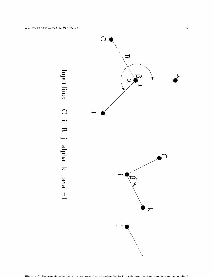
6.4. ZMATRIX — Z-MATRIX INPUT 67
������������
���
���
��
��
��
��
��
��
�� ���� ��
������������
�� ���� ��
i
kβ
�� ���� ��C
j
αR
j
k
C
i β
Input line: C i R
j alpha k beta +1
Figure 6.2: Relationships between the centers and two bond angles in Z-matrix input with optional parameter specifiedas +1.

68 CHAPTER 6. GEOMETRIES
������������
������������
�� ���� ��
����
��
��
��
��
���
���
���
���
��
��
��
��
i
kβ
�� ���� ��C
j
αR
j
k
i
β
C
Input line: C i R
j alpha k beta -1
Figure 6.3: Relationships between the centers and two bond angles in Z-matrix input with optional parameter specifiedas −1.

6.4. ZMATRIX — Z-MATRIX INPUT 69
CONSTANTS<string symbol> <real value>...
Each line contains the name of a variable followed by its value. As with the VARIABLES directive, an equals sign (=)can be included between the symbol and its value.
The end of the Z-matrix input using the compound ZMATRIX directive is signaled by a line containing either ENDor ZEND, following all input for the directive itself and its associated optional directives.
A simple example is presented for water. All Z-matrix parameters are specified numerically, and symbolic tags areused to specify connectivity information. This requires that all tags be unique, and therefore different tags are used forthe two hydrogen atoms, which may or may not be identical.
geometryzmatrix
OH1 O 0.95H2 O 0.95 H1 108.0
endend
The following example illustrates the Z-matrix input for the molecule CH3CF3. This input uses the numbers ofcenters to specify the connectivity information (i, j, and k), and uses symbolic variables for the Z-matrix parametersR, alpha, and beta, which are defined in the inputs for the VARIABLES and CONSTANTS directives.
geometryzmatrix
CC 1 CCH 1 CH1 2 HCH1H 1 CH2 2 HCH2 3 TOR1H 1 CH3 2 HCH3 3 -TOR2F 2 CF1 1 CCF1 3 TOR3F 2 CF2 1 CCF2 6 FCH1F 2 CF3 1 CCF3 6 -FCH1variables
CC 1.4888CH1 1.0790CH2 1.0789CH3 1.0789CF1 1.3667CF2 1.3669CF3 1.3669
constantsHCH1 104.28HCH2 104.74HCH3 104.7CCF1 112.0713CCF2 112.0341CCF3 112.0340TOR1 109.3996

70 CHAPTER 6. GEOMETRIES
TOR2 109.3997TOR3 180.0000FCH1 106.7846
endend
The input for any centers specified with Cartesian coordinates must be specified using the format of the <tag>lines described in Section 6.3 above. However, in order to correctly specify these Cartesian coordinates within theZ-matrix, the user must understand the orientation of centers specified using internal coordinates. These are arrangedas follows:
• The first center is placed at the origin.
• The second center is placed along the positive z-axis.
• The third center is placed in the z-x plane.
6.5 ZCOORD — Forcing internal coordinates
By default redundant internal coordinates are generated for use in geometry optimizations. Connectivity is inferredby comparing inter-atomic distances with the sum of the van der Waals radii of the two atoms involved in a possiblebond, times a scaling factor. The scaling factor is an input parameter of ZCOORDwhich maybe changed from its defaultvalue of 1.3. Under some circumstances (unusual bonding, bond dissociation, . . . ) it will be necessary to augmentthe automatically generated list of internal coordinates to force some specific internal coordinates to be included inamong the internal coordinates. This is accomplished by including the optional directive ZCOORD within the geometrydirective. The general form of the ZCOORD directive is as follows:
ZCOORDCVR_SCALING <real value>BOND <integer i> <integer j> \
[<real value>] [<string name>] [constant]ANGLE <integer i> <integer j> <integer k> \
[<real value>] [<string name>] [constant]TORSION <integer i> <integer j> <integer k> <integer l> \
[<real value>] [<string name>] [constant]END
The centers i, j, k and l must be specified using the numbers of the centers, as supplied in the input for theCartesian coordinates. The ZCOORD input parameters are defined as follows:
• cvr_scaling — scaling factor applied to van der Waals radii.
• bond — a bond between the two centers.
• angle — a bond angle i jk.
• torsion — a torsion (or dihedral) angle. The angle between the planes i-j-k and j-k-l.
A value may be specified for a user-defined internal coordinate, in which case it is forced upon the input Cartesiancoordinates while attempting to make only small changes in the other internal coordinates. If no value is provided the

6.6. APPLYING CONSTRAINTS IN GEOMETRY OPTIMIZATIONS 71
value implicit in the input coordinates is kept. If the keyword constant is specified, then that internal variable is notmodified during a geometry optimization with DRIVER (Section 20). Each internal coordinate may also be namedeither for easy identification in the output, or for the application of constraints (Section 6.6).
If the keyword adjust is specified on the main GEOMETRY directive, only ZCOORD data may be specified and itcan be used to change the user-defined internal coordinates, including adding/removing constraints and changing theirvalues.
6.6 Applying constraints in geometry optimizations
Internal coordinates specified as constant in a ZCOORD directive or in the constants section of a ZMATRIX directive,will be frozen at their initial values if a geometry optimization is performed with DRIVER (Section 20).
If internal coordinates have the same name (give or take an optional sign for torsions) then they are forced to havethe same value. This may be used to force bonds or angles to be equal even if they are not related by symmetry.
When atoms have been specified by their Cartesian coordinates, and internal coordinates are not being used, it ispossible to freeze the cartesian position of selected atoms. This is useful for such purposes as optimizing a moleculeabsorbed on the surface of a cluster with fixed geometry. Only the gradients associated with the active atoms arecomputed. This can result in a big computational saving, since gradients associated with frozen atoms are forced tozero (Note, however, that this destroys the translational and rotational invariance of the gradient. This is not yet fullyaccommodated by the STEPPER geometry optimization software, and can sometimes result in slower convergence ofthe optimization. The DRIVER optimization package does not suffer from this problem).
The SET directive (Section 5.7) is used to freeze atoms, by specifying a directive of the form:
set geometry:actlist <integer list_of_center_numbers>
This defines only the centers in the list as active. All other centers will have zero force assigned to them, and willremain frozen at their starting coordinates during a geometry optimization.
For example, the following directive specifies that atoms numbered 1, 5, 6, 7, 8, and 15 are active and all otheratoms are frozen:
set geometry:actlist 1 5:8 15
or equivalently,
set geometry:actlist 1 5 6 7 8 15
If this option is not specified by entering a SET directive, the default behavior in the code is to treat all atoms asactive. To revert to this default behavior after the option to define frozen atoms has been invoked, the UNSET directivemust be used (since the database is persistent, see Section 3.2). The form of the UNSET directive is as follows:
unset geometry:actlist
6.7 SYSTEM — Lattice parameters for periodic systems
This keyword is needed only for for 1-, 2-, and 3-dimensional periodic systems.
The system keyword can assume the following values

72 CHAPTER 6. GEOMETRIES
• polymer — system with 1-d translational symmetry.
• surface — system with 2-d translational symmetry.
• crystal — system with 3-d translational symmetry.
• molecule — no translational symmetry (this is the default)
When the system possess translational symmetry, fractional coordinates are used in the directions where trans-lational symmetry exists. This means that for crystals x, y and z are fractional, for surfaces x and y are fractional,whereas for polymers only z is fractional. For example, in the following H2O layer input (a 2-d periodic system), xand y coordinates are fractional, whereas z is expressed in Å.
geometry units angstromO 0.353553 0.353553 2.100000000H 0.263094 0.353553 2.663590000H 0.444007 0.353553 2.663590000
Since no space group symmetry is available yet other than P1, input of cell parameters is relative to the primitivecell. For example, this is the input required for the cubic face-centered type structure of bulk MgO.
system crystallat_a 2.97692 lat_b 2.97692 lat_c 2.97692alpha 60.00 beta 60.00 gamma 60.00
end

Chapter 7
Basis sets
NWChem currently supports basis sets consisting of generally contracted1 Cartesian Gaussian functions up to a max-imum angular momentum of six (h functions), and also sp (or L) functions2 . The BASIS directive is used to definethese, and also to specify use of an effective core potential (ECP) that is associated with a basis set; see Section 8.
The basis functions to be used for a given calculation can be drawn from a standard set in the EMSL basis setlibrary that is included in the release of NWChem (See Appendix A for a list of the standard basis sets currentlysupplied with the release of the code). Alternatively, the user can specify particular functions explicitly in the input, todefine a particular basis set.
The general form of the BASIS directive is as follows:
BASIS [<string name default "ao basis">] \[(spherical || cartesian) default cartesian] \[(segment || nosegment) default segment] \[(print || noprint) default print][rel]
<string tag> library [<string tag_in_lib>] \<string standard_set> [file <filename>] \[except <string tag list>] [rel]
...
<string tag> <string shell_type> [rel]<real exponent> <real list_of_coefficients>...
END
Examining the keywords on the first line of the BASIS directive:
• name1Generally contracted meaning that the same primitive, Gaussian functions are contracted into multiple contracted functions using different
contraction coefficients. Reuse of the radial functions increases the efficiency of integral generation.2An sp shell is two-component general contraction. However, the first component specifies an s shell and the second a p shell. Again, reuse of
the radial functions increases the efficiency of integral generation.
73

74 CHAPTER 7. BASIS SETS
By default, the basis set is stored in the database with the name "ao basis". Another name may be specifiedin the BASIS directive, thus, multiple basis sets may be stored simultaneously in the database. Also, the DFT(Section 11) and RI-MP2 (Section 16) modules and the Dyall-modified-Dirac relativistic method (Section 9.3)require multiple basis sets with specific names.
The user can associate the "ao basis" with another named basis using the SET directive (see Section 5.7).
• SPHERICAL or CARTESIAN
The keywords spherical and cartesian offer the option of using either spherical-harmonic (5 d, 7 f, 9 g,. . . ) or Cartesian (6 d, 10 f, 15 g, . . . ) angular functions. The default is Cartesian.
Note that the correlation-consistent basis sets were designed using spherical harmonics and to use these, thespherical keyword should be present in the BASIS directive. The use of spherical functions also helpseliminate problems with linear dependence.
• SEGMENT or NOSEGMENT
By default, NWChem forces all basis sets to be segmented, even if they are input with general contractions orL or sp shells. This is because the current derivative integral program cannot handle general contractions. If acalculation is computing energies only, a performance gain can result from exploiting generally contracted basissets, in which case NOSEGMENT should be specified.
• PRINT or NOPRINT
The default is for the input module to print all basis sets encountered. Specifying the keyword noprint allowsthe user to suppress this output.
• REL
This keyword marks the entire basis as a relativistic basis for the purposes of the Dyall-modified-Dirac rela-tivistic integral code. The marking of the basis set is necessary for the code to make the proper associationbetween the relativistic shells in the ao basis and the shells in the large and/or small component basis. This isonly necessary for basis sets which are to be used as the ao basis. The user is referred to Section 9.3 for moredetails.
Basis sets are associated with centers by using the tag of a center in a geometry that has either been input by theuser (Section 6) or is available elsewhere. Each atom or center with the same tag will have the same basis set. Allatoms must have basis functions assigned to them — only dummy centers (X or Bq) may have no basis functions. Tofacilitate the specification of the geometry and the basis set for any chemical system, the matching process of a basisset tag to a geometry tag first looks for an exact match. If no match is found, NWChem will attempt to match, ignoringcase, the name or symbol of the element. E.g., all hydrogen atoms in a system could be labeled “H1”, “H2”, . . . , inthe geometry but only one basis set specification for “H” or “hydrogen” is necessary. If desired, a special basis maybe added to one or more centers (e.g., “H1”) by providing a basis for that tag. If the matching mechanism fails thenNWChem stops with an appropriate error message.
A special set of tags, “*” and tags ending with a “*” (E.g. “H*”) can be used in combination with the keywordlibrary (see section below). These tags facilitate the definition of a certain type of basis set of all atoms, or a groupof atoms, in a geometry using only a single or very few basis set entries. The “*” tag will not place basis sets ondummy atoms, Bq* can be used for that if necessary.
Examined next is how to reference standard basis sets in the basis set library, and finally, how to define a basis setusing exponents and coefficients.

7.1. BASIS SET LIBRARY 75
7.1 Basis set library
The keyword library associated with each specific tag entry specifies that the calculation will use the standardbasis set in NWChem for that center. The variable <standard_set> is the name that identifies the functions in thelibrary. The names of standard basis sets are not case sensitive. See Appendix A for a complete list of the basis sets inthe NWChem library and their specifications.
The general form of the input line requesting basis sets from the NWChem basis set library is:
<string tag> library [<string tag_in_lib>] \<string standard set> [file < filename> \[except <string tag list>] [rel]
...
For example, the NWChem basis set library contains the Dunning cc-pvdz basis set. These may be used as follows
basisoxygen library cc-pvdzhydrogen library cc-pvdz
end
A default path of the NWChem basis set libraries is provided on installation of the code, but a different path can bedefined by specifying the keyword file, and one can explicitly name the file to be accessed for the basis functions.For example,
basiso library 3-21g file /usr/d3g681/nwchem/librarysi library 6-31g file /usr/d3g681/nwchem/libraries/
end
This directive tells the code to use the basis set 3-21g in the file /usr/d3g681/nwchem/library for atom oand to use the basis set 6-31g in the directory /usr/d3g681/nwchem/libraries/ for atom si, rather thanlook for them in the default libraries. When a directory is defined the code will search for the basis set in a file withthe name 6-31g.
The “*” tag can be used to efficiently define basis set input directives for large numbers of atoms. An example is:
basis
* library 3-21gend
This directive tells the code to assign the basis sets 3-21g to all the atom tags defined in the geometry. If one wantsto place a different basis set on one of the atoms defined in the geometry, the following directive can be used:
basis
* library 3-21g except Hend
This directive tells the code to assign the basis sets 3-21g to all the atoms in the geometry, except the hydrogenatoms. Remember that the user will have to explicitly define the hydrogen basis set in this directive! One may alsodefine tags that end with a “*”:

76 CHAPTER 7. BASIS SETS
basisoxy* library 3-21g
end
This directive tells the code to assign the basis sets 3-21g to all atom tags in the geometry that start with “oxy”.
If standard basis sets are to be placed upon a dummy center, the variable <tag_in_lib> must also be entered onthis line, to identify the correct atom type to use from the basis function library (see the ghost atom example in Section5.7 and below). For example: To specify the cc-pvdz basis for a calculation on the water monomer in the dimer basis,where the dummy oxygen and dummy hydrogen centers have been identified as bqo and bqh respectively, the BASISdirective is as follows:
basiso library cc-pvdzh library cc-pvdzbqo library o cc-pvdzbqh library h cc-pvdz
end
A special dummy center tag is bq*, which will assign the same basis set to all bq centers in the geometry. Just as withthe “*” tag, the except list can be used to assign basis sets to unique dummy centers.
The library basis sets can also be marked as relativistic by adding the rel keyword to the tag line. See Section 9.3for more details. The correlation consistent basis sets have been contracted for relativistic effects and are included inthe standard library.
There are also contractions in the standard library for both a point nucleus and a finite nucleus of Gaussian shape.These are usually distinguished by the suffixex _pt and _fi. It is the user’s responsibility to ensure that the con-traction matches the nuclear type specified in the geometry object. The specification of a finite nucleus basis set doesNOT automatically set the nuclear type for that atom to be finite. See Section 6 for information.
7.2 Explicit basis set definition
If the basis sets in the library or available in other external files are not suitable for a given calculation, the basis setmay be explicitly defined. A generally contracted Gaussian basis function is associated with a center using an inputline of the following form:
<string tag> <string shell_type> [rel]<real exponent> <real list_of_coefficients>...
The variable <shell_type> identifies the angular momentum of the shell, s, p, d, . . . . NWChem is configuredto handle up to h shells. The keyword rel marks the shell as relativistic — see Section 9.3 for more details. Subse-quent lines define the primitive function exponents and contraction coefficients. General contractions are specified byincluding multiple columns of coefficients.
The following example defines basis sets for the water molecule:
basis spherical nosegmentoxygen s

7.3. COMBINATIONS OF LIBRARY AND EXPLICIT BASIS SET INPUT 77
11720.0000 0.000710 -0.0001601759.0000 0.005470 -0.001263400.8000 0.027837 -0.006267113.7000 0.104800 -0.02571637.0300 0.283062 -0.07092413.2700 0.448719 -0.1654115.0250 0.270952 -0.1169551.0130 0.015458 0.5573680.3023 -0.002585 0.572759
oxygen s0.3023 1.000000
oxygen p17.7000 0.0430183.8540 0.2289131.0460 0.5087280.2753 0.460531
oxygen p0.2753 1.000000
oxygen d1.1850 1.000000
hydrogen s13.0100 0.0196851.9620 0.1379770.4446 0.4781480.1220 0.501240
hydrogen s0.1220 1.000000
hydrogen p0.7270 1.000000
oxygen s0.01 1.0
hydrogen s0.02974 1.0
hydrogen p0.141 1.0
end
7.3 Combinations of library and explicit basis set input
The user can use a mixture of library basis and explicit basis set input to define the basis sets used on the variousatoms.
For example, the following BASIS directive augments the Dunning cc-pvdz basis set for the water molecule witha diffuse s-shell on oxygen and adds the aug-cc-pVDZ diffuse functions onto the hydrogen.
basis spherical nosegmentoxygen library cc-pvdzhydrogen library cc-pvdzoxygen s
0.01 1.0

78 CHAPTER 7. BASIS SETS
hydrogen library "aug-cc-pVDZ Diffuse"end
The resulting basis set defined is identical to the one defined above in the explicit basis set input.

Chapter 8
Effective Core Potentials
Effective core potentials (ECPs) are a useful means of replacing the core electrons in a calculation with an effectivepotential, thereby eliminating the need for the core basis functions, which usually require a large set of Gaussians todescribe them. In addition to replacing the core, they may be used to represent relativistic effects, which are largelyconfined to the core. In this context, both the scalar (spin-free) relativistic effects and spin-orbit (spin-dependent)relativistic effects may be included in effective potentials. NWChem has the facility to use both, and these are describedin the next two sections.
A brief recapitulation of the development of RECPs is given here, following Pacios and Christiansen1. The processcan be viewed as starting from an atomic Dirac-Hartree-Fock calculation, done in jj coupling, and producing relativisticeffective potentials (REPs) for each l and j value, UREP
l j . From these, a local potential is extracted, which for examplecontains the Coulomb potential of the core electrons balanced by the part of the nuclear attraction which cancels thecore electron charge. The residue is expressed in a semi-local form,
UREP =UREPLJ (r)+
L−1
∑l=0
l+1/2
∑j=|l−1/2
[UREP
l j (r)−UREPLJ (r)
]∑m|l jm〉〈l jm| (8.1)
where L is one larger than the maximum angular momentum in the atom. The scalar potential is obtained by averagingthe REPs for each j for a given l to give an averaged relativistic effective potential, or AREP,
UAREPl (r) =
12l +1
[lUREP
l−1/2(r)+(l +1)UREPl+1/2(r)
]. (8.2)
These are summed into the full potential.
The spin-orbit potential is obtained from the difference between the REPs for the two j values for a given l, andmay be represented in terms of an effective spin-orbit operator,
HSO = s ·L−1
∑l=1
22l +1
∆UREPl ∑
mm′|lm〉〈lm|l|lm′〉〈lm′|. (8.3)
where
∆UREPl =UREP
l+1/2(r)−UREPl−1/2(r). (8.4)
1l. F. Pacios and P. A. Christiansen, J. Chem. Phys. 82, 2664 (1985)
79
80 CHAPTER 8. EFFECTIVE CORE POTENTIALS
The spin-orbit integrals generated by NWChem are the integrals over the sum, including the factor of 2/(2l + 1), sothat they may be treated as an effective spin-orbit operator without further factors introduced.
The effective potentials, both scalar and spin-orbit, are fitted to Gaussians with the form
r2Ul(r) = ∑k
Alkrnlk e−Blkr2
where Alk is the contraction coefficient, nlk is the exponent of the “r” term (r-exponent), and Blk is the Gaussianexponent. The nlk is shifted by 2, in accordance with most of the ECP literature and implementations, i.e., an nlk = 0implies r−2. The current implementation allows nlk values of only 0, 1, or 2.
8.1 Scalar ECPs
The optional directive ECP allows the user to describe an effective core potential (ECP) in terms of contracted Gaussianfunctions as given above. Potentials using these functions must be specified explicitly by user input in the ECPdirective. This directive has essentially the same form and properties as the standard BASIS directive, except foressential differences required for ECPs. Because of this, the ECP is treated internally as a basis set. The form of theinput for the ECP directive is as follows:
ECP [<string name default "ecp basis">] \[print || noprint default print]
<string tag> library [<string tag_in_lib>] \<string standard_set> [file <filename>] \[except <string tag list>]
<string tag> [nelec] <integer number_of_electrons_replaced>
...
<string tag> <string shell_type><real r-exponent> <real Gaussian-exponent> <real list_of_coefficients>
...
END
ECPs are automatically segmented, even if general contractions are input. The projection operators defined in anECP are spherical by default, so there is no need to include the CARTESIAN or SPHERICAL keyword as there is fora standard basis set. ECPs are associated with centers in geometries through tags or names of centers. These tags mustmatch in the same manner as for basis sets the tags in a GEOMETRY and ECP directives, and are limited to sixteen(16) characters. Each center with the same tag will have the same ECP. By default, the input module prints each ECPthat it encounters. The NOPRINT option can be used to disable printing. There can be only one active ECP, eventhough several may exist in the input deck. The ECP modules load “ecp basis” inputs along with any “ao basis” inputspresent. ECPs may be used in both energy and gradient calculations.
ECPs are named in the same fashion as geometries or regular basis sets, with the default name being "ecp basis".It should be clear from the above discussion on geometries and database entries how indirection is supported. All di-rectives that are in common with the standard Gaussian basis set input have the same function and syntax.

8.1. SCALAR ECPS 81
As for regular basis sets, ECPs may be obtained from the standard library. The names of the sets of ECPs availablein the standard library (their coverage is described in Appendix A) are
• "Hay-Wadt MB (n+1) ECP"
• "Hay-Wadt VDZ (n+1) ECP"
• "LANL2DZ ECP"
• "SBKJC VDZ ECP"
• "Stuttgart RLC ECP"
• "Stuttgart RSC ECP"
• "CRENBL ECP"
• "CRENBS ECP"
The keyword nelec allows the user to specify the number of core electrons replaced by the ECP. Additional inputlines define the specific coefficients and exponents. The variable <shell_type> is used to specify the componentsof the ECP. The keyword ul entered for <shell_type> denotes the local part of the ECP. This is equivalent to thehighest angular momentum functions specified in the literature for most ECPs. The standard entries (s, p, d, etc.)for shell_type specify the angular momentum projector onto the local function. The shell type label of s indicatesthe ul-s projector input, p indicates the ul-p, etc.
For example, the Christiansen, Ross and Ermler ARECPs are available in the standard basis set libary named{crenbl_ecp}. To perform a calculation on uranyl (UO2+
2 ) with all-electron oxygen (aug-cc-pvdz basis), anduranium with an ARECP and using the corresponding basis the following input can be used
geometryU 0 0 0O 0 0 1.65O 0 0 -1.65
endbasis
U library crenbl_ecpO library aug-cc-pvdz
endecp
U library crenbl_ecpend
The following is an example of explicit input of an ECP for H2CO. It defines an ECP for the carbon and oxygenatoms in the molecule.
ecpC nelec 2 # ecp replaces 2 electrons on CC ul # d
1 80.0000000 -1.600000001 30.0000000 -0.400000002 0.5498205 -0.03990210
C s # s - d

82 CHAPTER 8. EFFECTIVE CORE POTENTIALS
0 0.7374760 0.638108320 135.2354832 11.009162302 8.5605569 20.13797020
C p # p - d2 10.6863587 -3.246842802 23.4979897 0.78505765
O nelec 2 # ecp replaces 2 electrons on OO ul # d
1 80.0000000 -1.600000001 30.0000000 -0.400000002 1.0953760 -0.06623814
O s # s - d0 0.9212952 0.395521790 28.6481971 2.516548432 9.3033500 17.04478500
O p # p - s2 52.3427019 27.977907702 30.7220233 -16.49630500
end
Various ECPs without a local function are available, including those of the Stuttgart group. For those, no "ul" partneeds to be defined. To define the absence of the local potential, simply specify one contraction with a zero coefficient:
<string tag> ul2 1.00000 0.00000
8.2 Spin-orbit ECPs
The Spin-orbit ECPs can be used with the Density Functional Approach, but one has to run the calculations withoutsymmetry. Note: when a Hartree-Fock method is specified the spin-orbit input will be ignored.
Spin-orbit ECPs are fitted in precisely the same functional form as the scalar RECPs and have the same properties,with the exception that there is no local potential ul, no s potential and no effective charge has to be defined. Spin-orbitpotentials are specified in the same way as ECPs except that the directive SO is used instead of ECP. Note that therecurrently are no spin-orbit ECPs defined in the standard NWChem library. The SO directive is as follows:
SO [<string name default "so basis">] \[print || noprint default print]
<string tag> library [<string tag_in_lib>] \<string standard_set> [file <filename>][except <string tag list>]
...
<string tag> <string shell_type><real r-exponent> <real Gaussian-exponent> <real list_of_coefficients>
...
END

8.2. SPIN-ORBIT ECPS 83
Note: in the literature the coefficients of the spin-orbit potentials are NOT always defined in the same manner. TheNWChem code assumes that the spin-orbit potential defined in the input is of the form:
∆UNWCheml =
22l +1
∆Ul (8.5)
For example, in the literature the Stuttgart potentials are defined as ∆Ul and, hence, have to be multiplied by 2/(2l+1).On the other hand, the CRENBL potentials in the published papers are defined as l
2l+1 ∆Ul and, hence, have to bemultiplied by 2/l (Warning: on the CRENBL website the spin-orbit potentials already have been corrected with the2/l factor).

84 CHAPTER 8. EFFECTIVE CORE POTENTIALS

Chapter 9
Relativistic All-electron Approximations
All methods which include treatment of relativistic effects are ultimately based on the Dirac equation, which has a fourcomponent wave function. The solutions to the Dirac equation describe both positrons (the “negative energy” states)and electrons (the “positive energy” states), as well as both spin orientations, hence the four components. The wavefunction may be broken down into two-component functions traditionally known as the large and small components;these may further be broken down into the spin components.
The implementation of approximate all-electron relativistic methods in quantum chemical codes requires the re-moval of the negative energy states and the factoring out of the spin-free terms. Both of these may be achieved using atransformation of the Dirac Hamiltonian known in general as a Foldy-Wouthuysen transformation. Unfortunately thistransformation cannot be represented in closed form for a general potential, and must be approximated. One popularapproach is that originally formulated by Douglas and Kroll1 and developed by Hess2. This approach decouples thepositive and negative energy parts to second order in the external potential (and also fourth order in the fine structureconstant, α). Other approaches include the Zeroth Order Regular Approximation (ZORA)3 and modification of theDirac equation by Dyall4, and involves an exact FW transformation on the atomic basis set level5.
Since these approximations only modify the integrals, they can in principle be used at all levels of theory. Atpresent the Douglas-Kroll and ZORA implementations can be used at all levels of theory whereas Dyall’s approachis currently available at the Hartree-Fock level. The derivatives have been implemented, allowing both methods to beused in geometry optimizations and frequency calculations.
The RELATIVISTIC directive provides input for the implemented relativistic approximations and is a compounddirective that encloses additional directives specific to the approximations:
RELATIVISTIC[DOUGLAS-KROLL [<string (ON||OFF) default ON> \
<string (FPP||DKH||DKFULL||DK3||DK3FULL) default DKH>] ||ZORA [ (ON || OFF) default ON ] ||DYALL-MOD-DIRAC [ (ON || OFF) default ON ]
[ (NESC1E || NESC2E) default NESC1E ] ][CLIGHT <real clight default 137.0359895>]
END
1M. Douglas and N. M. Kroll, Ann. Phys. (N.Y.) 82, 89 (1974)2B.A. Hess, Phys. Rev. A 32, 756 (1985); 33, 3742 (1986)3C. Chang, M. Pelissier, M. Durand, Physica Scripta 34, 294 (1986); E. van Lenthe, The ZORA Equation, doctoral thesis, Vrije Universiteit,
Amsterdam (1996); S. Faas, J.G. Snijders, J.H. van Lenthe, E. van Lenthe, and E.J. Baerends, Chem. Phys. Lett. 246, 632 (1995).4K. G. Dyall, J. Chem. Phys. 100, 2118 (1994)5K. G. Dyall, J. Chem. Phys. 106, 9618 (1997); K. G. Dyall and T. Enevoldsen, J. Chem. Phys. 111, 10000 (1999).
85
86 CHAPTER 9. RELATIVISTIC ALL-ELECTRON APPROXIMATIONS
Only one of the methods may be chosen at a time. If both methods are found to be on in the input block, NWChemwill stop and print an error message. There is one general option for both methods, the definition of the speed of lightin atomic units:
CLIGHT <real clight default 137.0359895>
The following sections describe the optional sub-directives that can be specified within the RELATIVISTICblock.
9.1 Douglas-Kroll approximation
The spin-free and spin-orbit one-electron Douglas-Kroll approximation have been implemented. The use of relativisticeffects from this Douglas-Kroll approximation can be invoked by specifying:
DOUGLAS-KROLL [<string (ON||OFF) default ON> \<string (FPP||DKH||DKFULL|DK3|DK3FULL) default DKH>]
The ON|OFF string is used to turn on or off the Douglas-Kroll approximation. By default, if the DOUGLAS-KROLLkeyword is found, the approximation will be used in the calculation. If the user wishes to calculate a non-relativisticquantity after turning on Douglas-Kroll, the user will need to define a new RELATIVISTIC block and turn the ap-proximation OFF. The user could also simply put a blank RELATIVISTIC block in the input file and all options willbe turned off.
The FPP is the approximation based on free-particle projection operators6 whereas the DKH and DKFULL approx-imations are based on external-field projection operators7. The latter two are considerably better approximations thanthe former. DKH is the Douglas-Kroll-Hess approach and is the approach that is generally implemented in quantumchemistry codes. DKFULL includes certain cross-product integral terms ignored in the DKH approach (see for exampleHäberlen and Rösch8). The third-order Douglas-Kroll approximation has been implemented by T. Nakajima and K.Hirao9. This approximation can be called using DK3 (DK3 without cross-product integral terms) or DK3FULL (DK3with cross-product integral terms).
The contracted basis sets used in the calculations should reflect the relativistic effects, i.e. one should use con-tracted basis sets which were generated using the Douglas-Kroll Hamiltonian. Basis sets that were contracted usingthe non-relativistic (Schödinger) Hamiltonian WILL PRODUCE ERRONEOUS RESULTS for elements beyond thefirst row. See appendix A for available basis sets and their naming convention.
NOTE: we suggest that spherical basis sets are used in the calculation. The use of high quality cartesian basis setscan lead to numerical inaccuracies.
In order to compute the integrals needed for the Douglas-Kroll approximation the implementation makes use of afitting basis set (see literature given above for details). The current code will create this fitting basis set based on thegiven "ao basis" by simply uncontracting that basis. This again is what is commonly implemented in quantumchemistry codes that include the Douglas-Kroll method. Additional flexibility is available to the user by explicitlyspecifying a Douglas-Kroll fitting basis set. This basis set must be named "D-K basis" (see Chapter 7).
6B.A. Hess, Phys. Rev. A 32, 756 (1985)7B.A. Hess, Phys. Rev. A 33, 3742 (1986)8O.D. Häberlen, N. Rösch, Chem. Phys. Lett. 199, 491 (1992)9T. Nakajima and K. Hirao, Chem. Phys. Lett. 329, 5111 (2000); T. Nakajima and K. Hirao, J. Chem. Phys. 113, 7786 (2000)

9.2. ZEROTH ORDER REGULAR APPROXIMATION (ZORA) 87
9.2 Zeroth Order regular approximation (ZORA)
The spin-free and spin-orbit one-electron zeroth-order regular approximation (ZORA) have been implemented. Theuse of relativistic effects with ZORA can be invoked by specifying:
ZORA [<string (ON||OFF) default ON>
The ON|OFF string is used to turn on or off ZORA. By default, if the ZORA keyword is found, the approximationwill be used in the calculation. If the user wishes to calculate a non-relativistic quantity after turning on ZORA, theuser will need to define a new RELATIVISTIC block and turn the approximation OFF. The user can also simply puta blank RELATIVISTIC block in the input file and all options will be turned off.
9.3 Dyall’s Modified Dirac Hamitonian approximation
The approximate methods described in this section are all based on Dyall’s modified Dirac Hamiltonian. This Hamil-tonian is entirely equivalent to the original Dirac Hamiltonian, and its solutions have the same properties. The modifi-cation is achieved by a transformation on the small component, extracting out σ ·p/2mc. This gives the modified smallcomponent the same symmetry as the large component, and in fact it differs from the large component only at orderα2. The advantage of the modification is that the operators now resemble the operators of the Breit-Pauli Hamiltonian,and can be classified in a similar fashion into spin-free, spin-orbit and spin-spin terms. It is the spin-free terms whichhave been implemented in NWChem, with a number of further approximations.
The first is that the negative energy states are removed by a normalized elimination of the small component(NESC), which is equivalent to an exact Foldy-Wouthuysen (EFW) transformation. The number of components inthe wave function is thereby effectively reduced from 4 to 2. NESC on its own does not provide any advantages, andin fact complicates things because the transformation is energy-dependent. The second approximation therefore per-forms the elimination on an atom-by-atom basis, which is equivalent to neglecting blocks which couple different atomsin the EFW transformation. The advantage of this approximation is that all the energy dependence can be included inthe contraction coefficients of the basis set. The tests which have been done show that this approximation gives resultswell within chemical accuracy. The third approximation neglects the commutator of the EFW transformation with thetwo-electron Coulomb interaction, so that the only corrections that need to be made are in the one-electron integrals.This is the equivalent of the Douglas-Kroll(-Hess) approximation as it is usually applied.
The use of these approximations can be invoked with the use of the DYALL-MOD-DIRAC directive in the RELATIVISTICdirective block. The syntax is as follows.
DYALL-MOD-DIRAC [ (ON || OFF) default ON ][ (NESC1E || NESC2E) default NESC1E ]
The ON|OFF string is used to turn on or off the Dyall’s modified Dirac approximation. By default, if theDYALL-MOD-DIRAC keyword is found, the approximation will be used in the calculation. If the user wishesto calculate a non-relativistic quantity after turning on Dyall’s modified Dirac, the user will need to define a newRELATIVISTIC block and turn the approximation OFF. The user could also simply put a blank RELATIVISTICblock in the input file and all options will be turned off.
Both one- and two-electron approximations are available NESC1E || NESC2E, and both have analytic gradi-ents. The one-electron approximation is the default. The two-electron approximation specified by NESC2E has somesub options which are placed on the same logical line as the DYALL-MOD-DIRAC directive, with the following syntax:
NESC2E [ (SS1CENT [ (ON || OFF) default ON ] || SSALL) default SSALL ]

88 CHAPTER 9. RELATIVISTIC ALL-ELECTRON APPROXIMATIONS
[ (SSSS [ (ON || OFF) default ON ] || NOSSSS) default SSSS ]
The first sub-option gives the capability to limit the two-electron corrections to those in which the small com-ponents in any density must be on the same center. This reduces the (LL|SS) contributions to at most three-centerintegrals and the (SS|SS) contributions to two centers. For a case with only one relativistic atom this option is redun-dant. The second controls the inclusion of the (SS|SS) integrals which are of order α4. For light atoms they may safelybe neglected, but for heavy atoms they should be included.
In addition to the selection of this keyword in the RELATIVISTIC directive block, it is necessary to supplybasis sets in addition to the ao basis. For the one-electron approximation, three basis sets are needed: the atomicFW basis set, the large component basis set and the small component basis set. The atomic FW basis set should beincluded in the ao basis. The large and small components should similarly be incorporated in basis sets namedlarge component and small component, respectively. For the two-electron approximation, only two basissets are needed. These are the large component and the small component. The large component should be includedin the ao basis and the small component is specified separately as small component, as for the one-electronapproximation. This means that the two approximations can not be run correctly without changing the ao basis,and it is up to the user to ensure that the basis sets are correctly specified.
There is one further requirement in the specification of the basis sets. In the ao basis, it is necessary to addthe rel keyword either to the basis directive or the library tag line (See below for examples). The former marksthe basis functions specified by the tag as relativistic, the latter marks the whole basis as relativistic. The markingis actually done at the unique shell level, so that it is possible not only to have relativistic and nonrelativistic atoms,it is also possible to have relativistic and nonrelativistic shells on a given atom. This would be useful, for example,for diffuse functions or for high angular momentum correlating functions, where the influence of relativity was small.The marking of shells as relativistic is necessary to set up a mapping between the ao basis and the large and/or smallcomponent basis sets. For the one-electron approximation the large and small component basis sets MUST be of thesame size and construction, i.e. differing only in the contraction coefficients.
It should also be noted that the relativistic code will NOT work with basis sets that contain sp shells, nor will itwork with ECPs. Both of these are tested and flagged as an error.
Some examples follow. The first example sets up the data for relativistic calculations on water with the one-electronapproximation and the two-electron approximation, using the library basis sets.
start h2o-dmd
geometry units bohrsymmetry c2v
O 0.000000000 0.000000000 -0.009000000H 1.515260000 0.000000000 -1.058900000H -1.515260000 0.000000000 -1.058900000
end
basis "fw" reloxygen library cc-pvdz_pt_sf_fwhydrogen library cc-pvdz_pt_sf_fw
end
basis "large"oxygen library cc-pvdz_pt_sf_lchydrogen library cc-pvdz_pt_sf_lc
end

9.3. DYALL’S MODIFIED DIRAC HAMITONIAN APPROXIMATION 89
basis "large2" reloxygen library cc-pvdz_pt_sf_lchydrogen library cc-pvdz_pt_sf_lc
end
basis "small"oxygen library cc-pvdz_pt_sf_schydrogen library cc-pvdz_pt_sf_sc
end
set "ao basis" fwset "large component" largeset "small component" small
relativisticdyall-mod-dirac
end
task scf
set "ao basis" large2unset "large component"set "small component" small
relativisticdyall-mod-dirac nesc2e
end
task scf
The second example has oxygen as a relativistic atom and hydrogen nonrelativistic.
start h2o-dmd2
geometry units bohrsymmetry c2v
O 0.000000000 0.000000000 -0.009000000H 1.515260000 0.000000000 -1.058900000H -1.515260000 0.000000000 -1.058900000
end
basis "ao basis"oxygen library cc-pvdz_pt_sf_fw relhydrogen library cc-pvdz
end
basis "large component"oxygen library cc-pvdz_pt_sf_lc
end
basis "small component"

90 CHAPTER 9. RELATIVISTIC ALL-ELECTRON APPROXIMATIONS
oxygen library cc-pvdz_pt_sf_scend
relativisticdyall-mod-dirac
end
task scf
Chapter 10
Hartree-Fock or Self-consistent Field
The NWChem self-consistent field (SCF) module computes closed-shell restricted Hartree-Fock (RHF) wavefunc-tions, restricted high-spin open-shell Hartree-Fock (ROHF) wavefunctions, and spin-unrestricted Hartree-Fock (UHF)wavefunctions.
The SCF directive provides input to the SCF module and is a compound directive that encloses additional directivesspecific to the SCF module:
SCF...
END
10.1 Wavefunction type
A spin-restricted, closed shell RHF calculation is performed by default. An error results if the number of electrons isinconsistent with this assumption. The number of electrons is inferred from the total charge on the system and the sumof the effective nuclear charges of all centers (atoms and dummy atoms, Section 6). The total charge on the system iszero by default, unless specified at some value by input on the CHARGE directive (Section 5).
The options available to define the SCF wavefunction and multiplicity are as follows:
SINGLETDOUBLETTRIPLETQUARTETQUINTETSEXTETSEPTETOCTETNOPEN <integer nopen default 0>RHFROHFUHF
The optional keywords SINGLET, DOUBLET, . . . , OCTET and NOPEN allow the user to specify the number of
91

92 CHAPTER 10. HARTREE-FOCK OR SELF-CONSISTENT FIELD
singly occupied orbitals for a particular calculation. SINGLET is the default, and specifies a closed shell; DOUBLETspecifies one singly occupied orbital; TRIPLET specifies two singly occupied orbitals; and so forth. If there are morethan seven singly occupied orbitals, the keyword NOPEN must be used, with the integer nopen defining the numberof singly occupied orbitals (sometimes referred to as open shells).
If the multiplicity is any value other than SINGLET, the default calculation will be a spin-restricted, high-spin,open-shell SCF calculation (keyword ROHF). The open-shell orbitals must be the highest occupied orbitals. If nec-essary, any starting vectors may be rearranged through the use of the SWAP keyword on the VECTORS directive (seeSection 10.5) to accomplish this.
A spin-unrestricted solution can also be performed by specifying the keyword UHF. In UHF calculations, it isassumed that the number of singly occupied orbitals corresponds to the difference between the number of alpha-spinand beta-spin orbitals. For example, a UHF calculation with 2 more alpha-spin orbitals than beta-spin orbitals can beobtained by specifying
scftriplet ; uhf # (Note: two logical lines of input)...
end
The user should be aware that, by default, molecular orbitals are symmetry adapted in NWChem. This may notbe desirable for fully unrestricted wavefunctions. In such cases, the user has the option of defeating the defaults byspecifying the keywords ADAPT OFF (see Section 10.3) and SYM OFF (see Section 10.2).
The keywords RHF and ROHF are provided in the code for completeness. It may be necessary to specify these inorder to modify the behavior of a previous calculation (see Section 3.2 for restart behavior).
10.2 SYM — use of symmetry
SYM <string (ON||OFF) default ON>
This directive enables/disables the use of symmetry to speed up Fock matrix construction (via the petite-list orskeleton algorithm) in the SCF, if symmetry was used in the specification of the geometry. Symmetry adaptation ofthe molecular orbitals is not affected by this option. The default is to use symmetry if it is specified in the geometrydirective (Section 6).
For example, to disable use of symmetry in Fock matrix construction:
sym off
10.3 ADAPT – symmetry adaptation of MOs
ADAPT <string (ON||OFF) default ON>
The default in the SCF module calculation is to force symmetry adaption of the molecular orbitals. This does notaffect the speed of the calculation, but without explicit adaption the resulting orbitals may be symmetry contaminatedfor some problems. This is especially likely if the calculation is started using orbitals from a distorted geometry.

10.4. TOL2E — INTEGRAL SCREENING THRESHOLD 93
The underlying assumption in the use of symmetry in Fock matrix construction is that the density is totally sym-metric. If the orbitals are symmetry contaminated, this assumption may not be valid — which could result in incorrectenergies and poor convergence of the calculation. It is thus advisable when specifying ADAPT OFF to also specifySYM OFF (Section 10.2).
10.4 TOL2E — integral screening threshold
TOL2E <real tol2e default min(10e-7 , 0.01*$thresh$)>
The variable tol2e is used in determining the integral screening threshold for the evaluation of the energy andrelated Fock-like matrices. The Schwarz inequality is used to screen the product of integrals and density matrices in amanner that results in an accuracy in the energy and Fock matrices that approximates the value specified for tol2e.
It is generally not necessary to set this parameter directly. Specify instead the required precision in the wavefunc-tion, using the THRESH directive (Section 10.7). The default threshold is the minimum of 10−7 and 0.01 times therequested convergence threshold for the SCF calculation (Section 10.7).
The input to specify the threshold explicitly within the SCF directive is, for example:
tol2e 1e-9
For very diffuse basis sets, or for high-accuracy calculations it might be necessary to set this parameter. A valueof 10−12 is sufficient for nearly all such purposes.
10.5 VECTORS — input/output of MO vectors
VECTORS [[input] (<string input_movecs default atomic>) || \(project <string basisname> <string filename>) || \(fragment <string file1> [<string file2> ...])] \
[swap [alpha||beta] <integer vec1 vec2> ...] \[reorder <integer atom1 atom2> ...] \[output <string output_filename default input_movecs>] \[lock][rotate <string input_geometry> <string input_movecs>]
The VECTORS directive allows the user to specify the source and destination of the molecular orbital vectors. Ina startup calculation (see Section 5.1), the default source for guess vectors is a diagonalized Fock matrix constructedfrom a superposition of the atomic density matrices for the particular problem. This is usually a very good guess. Fora restarted calculation, the default is to use the previous MO vectors.
The optional keyword INPUT allows the user to specify the source of the input molecular orbital vectors as any ofthe following:
• ATOMIC — eigenvectors of a Fock-like matrix formed from a superposition of the atomic densities (the defaultguess). See Sections 10.5.2 and 10.6.
• HCORE — eigenvectors of the bare-nucleus Hamiltonian or the one-electron Hamiltonian.

94 CHAPTER 10. HARTREE-FOCK OR SELF-CONSISTENT FIELD
• filename — the name of a file containing the MO vectors from a previous calculation. Note that unless thepath is fully qualified, or begins with a dot (“.”), then it is assumed to reside in the directory for permanent files(see Section 5.2).
• PROJECT basisname filename — projects the existing MO vectors in the file filename from thesmaller basis with name basisname into the current basis. The definition of the basis basisname must beavailable in the current database, and the basis must be smaller than the current basis. In addition, the geometryused for the previous calculations must have the atoms in the same order and in the same orientation as thecurrent geometry.
• FRAGMENT file1 ... — assembles starting MO vectors from previously performed calculations on frag-ments of the system and is described in more detail in Section 10.5.1. Even though there are some significantrestrictions in the use of the initial implementation of this method (see Section 10.5.1), this is the most powerfulinitial guess option within the code. It is particularly indispensable for open shell metallic systems.
• ROTATE input_geometry input_movecs — rotates MO vectors generated at a previous geometry tothe current active geometry.
The molecular orbitals are saved every iteration if more than 600 seconds have elapsed, and also at the end of thecalculation. At completion (converged or not), the SCF module always canonically transforms the molecular orbitalsby separately diagonalizing the closed–closed, open–open, and virtual–virtual blocks of the Fock matrix.
The name of the file used to store the MO vectors is determined as follows:
• if the OUTPUT keyword was specified on the VECTORS directive, then the filename that follows this keywordis used, or
• if the input vectors were read from a file, this file is reused for the output vectors (overwriting the input vectors);else,
• a default file name is generated in the directory for permanent files (Section 5.2) by prepending ".movecs"with the file prefix, i.e., "<file_prefix>.movecs".
The name of this file is stored in the database so that a subsequent SCF calculation will automatically restart fromthese MO vectors.
Applications of this directive are illustrated in the following examples.
Example 1:
vectors output h2o.movecs
Assuming a start-up calculation, this directive will result in use of the default atomic density guess, and will outputthe vectors to the file h2o.movecs.
Example 2:
vectors input initial.movecs output final.movecs
This directive will result in the initial vectors being read from the file "initial.movecs". The results will bewritten to the file final.movecs. The contents of "initial.movecs" will not be changed.
Example 3:
vectors input project "small basis" small.movecs

10.5. VECTORS — INPUT/OUTPUT OF MO VECTORS 95
This directive will cause the calculation to start from vectors in the file "small.movecs" which are in a basisnamed "small basis". The output vectors will be written to the default file "<file_prefix.movecs>".
Once starting vectors have been obtained using any of the possible options, they may be reordered through use ofthe SWAP keyword. This optional keyword requires a list of orbital pairs that will be swapped. For UHF calculations,separate SWAP keywords may be provided for the alpha and beta orbitals, as necessary.
An example of use of the SWAP directive:
vectors input try1.movecs swap 173 175 174 176 output try2.movecs
This directive will cause the initial orbitals to be read from the file "try1.movecs". The vectors for the orbitalswithin the pairs 173–175 will be swapped with those within 174–176, so the resulting order is 175, 176, 173, 174. Thefinal orbitals obtained in the calculation will be written to the file "try2.movecs".
The swapping of orbitals occurs as a sequential process in the order (left to right) input by the user. Thus, regardingeach pair as an elementary transposition it is possible to construct arbitrary permutations of the orbitals. For instance,to apply the permutation (6789)1 we note that this permutation is equal to (67)(78)(89), and thus may be specified as
vectors swap 8 9 7 8 6 7
Another example, now illustrating this feature for a UHF calculation, is the directive
vectors swap beta 4 5 swap alpha 5 6
This input will result in the swapping of the 5–6 alpha orbital pair and the 4–5 beta orbital pair. (All other items in theinput use the default values.)
The LOCK keyword allows the user to specify that the ordering of orbitals will be locked to that of the initial vectors,insofar as possible. The default is to order by ascending orbital energies within each orbital space. One applicationwhere locking might be desirable is a calculation where it is necessary to preserve the ordering of a previous geometry,despite flipping of the orbital energies. For such a case, the LOCK directive can be used to prevent the SCF calculationfrom changing the ordering, even if the orbital energies change.
The mapping of the MO’s to the nuclei can be changed using the REORDER keyword. Once starting vectors havebeen obtained using any of the possible options, the REORDER keyword moves the MO coefficients between atomslisted in the integer list. This keyword is particularly useful for calculating localized electron and hole states.
This optional keyword requires a list containing the new atom ordering. It is not necessary to provide separate listsfor alpha and beta orbitals.
An example of use of the REORDER keyword:
vectors input try1.movecs reorder 2 1 output try2.movecs
This directive will cause the initial orbitals to be read from the file "try1.movecs". The MO coefficients for thebasis functions on atom 2 will be swapped with those on atom 1. The final orbitals obtained in the calculation will bewritten to the file "try2.movecs".
The following example shows how the ROTATE keyword can be used to rotate MO vectors calculated at geometrygeom1 to geometry geom2, which has a different rotational orientation:
set geometry geom1
1The cyclic permutation (6789) maps the ordered list 6 7 8 9 into 9 6 7 8.

96 CHAPTER 10. HARTREE-FOCK OR SELF-CONSISTENT FIELD
dftvectors input atomic output geom1.mo
endtask dft
set geometry geom2dftvectors input rotate geom1 geom1.mo output geom2.mo
endtask dft
10.5.1 Superposition of fragment molecular orbitals
The fragment initial guess is particularly useful in the following instances:
• The system naturally decomposes into molecules that can be treated individually, e.g., a cluster.
• One or more fragments are particularly hard to converge and therefore much time can be saved by convergingthem independently.
• A fragment (e.g., a metal atom) must be prepared with a specific occupation. This can often be readily accom-plished with a calculation on the fragment using dummy charges to model a ligand field.
• The molecular occupation predicted by the atomic initial guess is often wrong for systems with heavy metalswhich may have partially occupied orbitals with lower energy than some doubly occupied orbitals. The fragmentinitial guess avoids this problem.
VECTORS [input] fragment <string file1> [<string file2> ...]
The molecular orbitals are formed by superimposing the previously generated orbitals of fragments of the moleculebeing studied. These fragment molecular orbitals must be in the same basis as the current calculation. The inputspecifies the files containing the fragment molecular orbitals. For instance, in a calculation on the water dimer, onemight specify
vectors fragment h2o1.movecs h2o2.movecs
where h2o1.movecs contains the orbitals for the first fragment, and h2o2.movecs contains the orbitals for thesecond fragment.
A complete example of the input for a calculation on the water dimer using the fragment guess is as follows:
start dimer
title "Water dimer SCF using fragment initial guess"
geometry dimerO -0.595 1.165 -0.048H 0.110 1.812 -0.170H -1.452 1.598 -0.154O 0.724 -1.284 0.034

10.5. VECTORS — INPUT/OUTPUT OF MO VECTORS 97
H 0.175 -2.013 0.348H 0.177 -0.480 0.010
end
geometry h2o1O -0.595 1.165 -0.048H 0.110 1.812 -0.170H -1.452 1.598 -0.154
end
geometry h2o2O 0.724 -1.284 0.034H 0.175 -2.013 0.348H 0.177 -0.480 0.010
end
basiso library 3-21gh library 3-21g
end
set geometry h2o1scf; vectors input atomic output h2o1.movecs; endtask scf
set geometry h2o2scf; vectors input atomic output h2o2.movecs; endtask scf
set geometry dimerscfvectors input fragment h2o1.movecs h2o2.movecs \
output dimer.movecsendtask scf
First, the geometry of the dimer and the two monomers are specified and given names. Then, after the basis specifi-cation, calculations are performed on the fragments by setting the geometry to the appropriate fragment (Section 5.7)and redirecting the output molecular orbitals to an appropriately named file. Note also that use of the atomic initialguess is forced, since the default initial guess is to use any existing MOs which would not be appropriate for the secondfragment calculation. Finally, the dimer calculation is performed by specifying the dimer geometry, indicating use ofthe fragment guess, and redirecting the output MOs.
The following points are important in using the fragment initial guess:
1. The fragment calculations must be in the same basis set as the full calculation.
2. The order of atoms in the fragments and the order in which the fragment files are specified must be such thatwhen the fragment basis sets are concatenated all the basis functions are in the same order as in the full system.This is readily accomplished by first generating the full geometry with atoms for each fragment contiguous, split-ting this into numbered fragments and specifying the fragment MO files in the correct order on the VECTORSdirective.

98 CHAPTER 10. HARTREE-FOCK OR SELF-CONSISTENT FIELD
3. The occupation of orbitals is preserved when they are merged from the fragments to the full molecule and theresulting occupation must match the requested occupation for the full molecule. E.g., a triplet ROHF calculationmust be comprised of fragments that have a total of exactly two open-shell orbitals.
4. Because of these restrictions, it is not possible to introduce additional atoms (or basis functions) into fragmentsfor the purpose of cleanly breaking real bonds. However, it is possible, and highly recommended, to introduceadditional point charges to simulate the presence of other fragments.
5. MO vectors of partially occupied or strongly polarized systems are very sensitive to orientation. While it ispossible to specify the same fragment MO vector file multiple times in the VECTORS directive, it is usuallymuch better to do a separate calculation for each fragment.
6. Linear dependencies which were present in a fragment calculation may be magnified in the full calculation.When this occurs, some of the fragment’s highest virtual orbitals will not be copied to the full system, and awarning will be printed.
A more involved example is now presented. We wish to model the sextet state of Fe(III) complexed with water,imidazole and a heme with a net unit positive charge. The default atomic guess does not give the correct d5 occupationfor the metal and also gives an incorrect state for the double anion of the heme. The following performs calculationson all of the fragments. Things to note are:
1. The use of a dummy +2 charge in the initial guess on the heme which in part simulates the presence of the metalion, and also automatically forces an additional two electrons to be added to the system (the default net chargebeing zero).
2. The iron fragment calculation (charge +3, d5, sextet) will yield the correct open-shell occupation for the fullsystem. If, instead, the d-orbitals were partially occupied (e.g., the doublet state) it would be useful to introducedummy charges around the iron to model the ligand field and thereby lift the degeneracy to obtain the correctoccupation.
3. Cs symmetry is used for all of the calculations. It is not necessary that the same symmetry be used in all of thecalculations, provided that the order and orientation of the atoms is preserved.
4. The unset scf:* directive is used immediately before the calculation on the full system so that the defaultname for the output MO vector file can be used, rather than having to specify it explicitly.
start heme6a1title "heme-H2O (6A1) from M.Dupuis"
############################################################# Define the geometry of the full system and the fragments #############################################################
geometry full-systemsymmetry cs
H 0.438 -0.002 4.549C 0.443 -0.001 3.457C 0.451 -1.251 2.828C 0.452 1.250 2.828H 0.455 2.652 4.586H 0.461 -2.649 4.586N1 0.455 -1.461 1.441

10.5. VECTORS — INPUT/OUTPUT OF MO VECTORS 99
N1 0.458 1.458 1.443C 0.460 2.530 3.505C 0.462 -2.530 3.506C 0.478 2.844 1.249C 0.478 3.510 2.534C 0.478 -2.848 1.248C 0.480 -3.513 2.536C 0.484 3.480 0.000C 0.485 -3.484 0.000H 0.489 4.590 2.664H 0.496 -4.592 2.669
H 0.498 4.573 0.000H 0.503 -4.577 0.000H -4.925 1.235 0.000H -4.729 -1.338 0.000C -3.987 0.685 0.000N -3.930 -0.703 0.000C -2.678 1.111 0.000C -2.622 -1.076 0.000H -2.284 2.126 0.000H -2.277 -2.108 0.000N -1.838 0.007 0.000
Fe 0.307 0.000 0.000
O 2.673 -0.009 0.000H 3.238 -0.804 0.000H 3.254 0.777 0.000
end
geometry ring-onlysymmetry csH 0.438 -0.002 4.549C 0.443 -0.001 3.457C 0.451 -1.251 2.828C 0.452 1.250 2.828H 0.455 2.652 4.586H 0.461 -2.649 4.586N1 0.455 -1.461 1.441N1 0.458 1.458 1.443C 0.460 2.530 3.505C 0.462 -2.530 3.506C 0.478 2.844 1.249C 0.478 3.510 2.534C 0.478 -2.848 1.248C 0.480 -3.513 2.536C 0.484 3.480 0.000C 0.485 -3.484 0.000H 0.489 4.590 2.664H 0.496 -4.592 2.669

100 CHAPTER 10. HARTREE-FOCK OR SELF-CONSISTENT FIELD
Bq 0.307 0.0 0.0 charge 2 # simulate the ironend
geometry imid-onlysymmetry csH 0.498 4.573 0.000H 0.503 -4.577 0.000H -4.925 1.235 0.000H -4.729 -1.338 0.000C -3.987 0.685 0.000N -3.930 -0.703 0.000C -2.678 1.111 0.000C -2.622 -1.076 0.000H -2.284 2.126 0.000H -2.277 -2.108 0.000N -1.838 0.007 0.000
end
geometry fe-onlysymmetry csFe .307 0.000 0.000
end
geometry water-onlysymmetry csO 2.673 -0.009 0.000H 3.238 -0.804 0.000H 3.254 0.777 0.000
end
############################# Basis set for everything #############################
basis nosegmentO library 6-31g*N library 6-31g*C library 6-31g*H library 6-31g*Fe library "Ahlrichs pVDZ"
end
########################################################### SCF on the fragments for initial guess for full system ###########################################################
scf; thresh 1e-2; end
set geometry ring-onlyscf; vectors atomic swap 80 81 output ring.mo; end

10.5. VECTORS — INPUT/OUTPUT OF MO VECTORS 101
task scf
set geometry water-onlyscf; vectors atomic output water.mo; endtask scf
set geometry imid-onlyscf; vectors atomic output imid.mo; endtask scf
charge 3set geometry fe-onlyscf; sextet; vectors atomic output fe.mo; endtask scf
########################### SCF on the full system ###########################
unset scf:* # This restores the defaults
charge 1
set geometry full-system
scfsextetvectors fragment ring.mo imid.mo fe.mo water.momaxiter 50
end
task scf
10.5.2 Atomic guess orbitals with charged atoms
As noted above, the default guess vectors are based on superimposing the density matrices of the neutral atoms. Ifsome atoms are significantly charged, this default guess may be improved upon by modifying the atomic densities.This is done by setting parameters that add fractional charges to the occupation of the valence atomic orbitals. Sincethe atomic SCF program does not have its own input block, the SET directive (Section 5.7) must be used to set theseparameters.
The input specifies a list of tags (i.e., names of atoms in a geometry, see Section 6) and the charges to be added tothose centers. Two parameters must be set as follows:
set atomscf:tags_z <string list_of_tags>set atomscf:z <real list_of_charges>
The array of strings atomscf:tags_z should be set to the list of tags, and the array atomscf:z should be setto the list of charges which must be real numbers (not integers). All atoms that have a tag specified in the list of tagswill be assigned the corresponding charge from the list of charges.
102 CHAPTER 10. HARTREE-FOCK OR SELF-CONSISTENT FIELD
For example, the following specifies that all oxygen atoms with tag O be assigned a charge of -1 and all iron atomswith tag Fe be assigned a charge of +2
set atomscf:z -1 2.0set atomscf:tags_z O Fe
There are some limitations to this feature. It is not possible to add electrons to closed shell atoms, nor is it possibleto remove all electrons from a given atom. Attempts to do so will cause the code to report an error, and it will notreport further errors in the input for modifying the charge even when they are detected.
Finally, recall that the database is persistent (Section 3.2) and that the modified settings will be used in subsequentatomic guess calculations unless the data is deleted from the database with the UNSET directive (Section 5.8).
10.6 Accuracy of initial guess
For SCF, the initial Fock-matrix construction from the atomic guess is now (staring from version 3.3) performed to adefault precision of 1e-7. However, other wavefunctions, notably DFT, use a lower precision. In charged, or diffusebasis sets, this precision may not be sufficient and could result in incorrect ordering of the initial orbitals. The accuracymay be increased with the following directive which should be inserted in the top-level of input (i.e., outside of theSCF input block) and before the TASK directive.
set tolguess 1e-7
10.7 THRESH — convergence threshold
THRESH <real thresh default 1.0e-4>
This directive specifies the convergence threshold for the calculation. The convergence threshold is the norm ofthe orbital gradient, and has a default value in the code of 10−4.
The norm of the orbital gradient corresponds roughly to the precision available in the wavefunction, and the energyshould be converged to approximately the square of this number. It should be noted, however, that the precision in theenergy will not exceed that of the integral screening tolerance. This tolerance (Section 10.4) is automatically set fromthe convergence threshold, so that sufficient precision is usually available by default.
The default convergence threshold suffices for most SCF energy and geometry optimization calculations, provid-ing about 6–8 decimal places in the energy, and about four significant figures in the density and energy derivativewith respect to nuclear coordinates. However, greater precision may be required for calculations involving weakly in-teracting systems, floppy molecules, finite-difference of gradients to compute the Hessian, and for post-Hartree-Fockcalculations. A threshold of 10−6 is adequate for most such purposes, and a threshold of 10−8 might be necessary forvery high accuracy or very weak interactions. A threshold of 10−10 should be regarded as the best that can be attainedin most circumstances.
10.8 MAXITER — iteration limit
MAXITER <integer maxiter default 8>

10.9. PROFILE — PERFORMANCE PROFILE 103
The maximum number of iterations for the SCF calculation defaults to 20 for both ROHF/RHF and UHF calcu-lations. For most molecules, this number of iterations is more than sufficient for the quadratically convergent SCFalgorithm to obtain a solution converged to the default threshold (see Section 10.7 above). If the SCF program detectsthat the quadratically convergent algorithm is not efficient, then it will resort to a linearly convergent algorithm andincrease the maximum number of iterations by 10.
Convergence may not be reached in the maximum number of iterations for many reasons, including input error(e.g., an incorrect geometry or a linearly dependent basis), a very low convergence threshold, a poor initial guess, orthe fact that the system is intrinsically hard to converge due to the presence of many states with similar energies.
The following sets the maximum number of SCF iterations to 50:
maxiter 50
10.9 PROFILE — performance profile
This directive allows the user to obtain timing and parallel execution information about the SCF module. It is specifiedby the simple keyword
PROFILE
This option can be helpful in understanding the computational performance of an SCF calculation. However, itcan introduce a significant overhead on machines that have expensive timing routines, such as the SUN.
10.10 DIIS — DIIS convergence
This directive allows the user to specify DIIS convergence rather than second-order convergence for the SCF calcula-tion. The form of the directive is as follows:
DIIS
The implementation of this option is currently fairly rudimentary. It does not have level-shifting and damping, anddoes not support open shells or UHF. It is provided on an “as is” basis, and should be used with caution.
When the DIIS directive is specified in the input, the user has the additional option of specifying the size of thesubspace for the DIIS extrapolation. This is accomplished with the DIISBAS directive, which is of the form:
DIISBAS <integer diisbas default 5>
The default of 5 should be adequate for most applications, but may be increased if convergence is poor. On largesystems, it may be necessary to specify a lower value for diisbas, to conserve memory.
10.11 DIRECT and SEMIDIRECT — recomputation of integrals
In the context of SCF calculations direct means that all integrals are recomputed as required and none are stored.The other extreme are disk- or memory-resident (sometimes termed conventional) calculations in which all integrals

104 CHAPTER 10. HARTREE-FOCK OR SELF-CONSISTENT FIELD
are computed once and stored. Semi-direct calculations are between these two extremes with some integrals beingprecomputed and stored, and all other integrals being recomputed as necessary.
The default behavior of the SCF module is
• If enough memory is available, the integrals are computed once and are cached in memory.
• If there is not enough memory to store all the integrals at once, then 95% of the available disk space in thescratch directory (see Section 5.2) is assumed to be available for this purpose, and as many integrals as possibleare cached on disk (with no memory being used for caching). Some attempt is made to store the most expensiveintegrals in the cache.
• If there is not enough room in memory or on disk for all the integrals, then the ones that are not cached arerecomputed in a semidirect fashion.
The integral file is deleted at the end of a calculation, so it is not possible to restart a semidirect calculation whenthe integrals are cached in memory or on disk. Many computer systems (e.g., the EMSL IBM SP) clear the fastscratch space at the end of each job, adding a further complication to the problem of restarting a parallel semidirectcalculation.
On the IBM SP or any other computer with fast disks local to each processor, semidirect calculation offers the bestbehavior. It can result in quadratic speedup as more processors are added.
A fully direct calculation (with recomputation of the integrals at each iteration) is forced by specifying the directive
DIRECT
Alternatively, the SEMIDIRECT directive can be used to control the default semidirect calculation by defining theamount of disk space and the cache memory size. The form of this directive is as follows:
SEMIDIRECT [filesize <integer filesize default disksize>][memsize <integer memsize default available>][filename <string filename default $file_prefix.aoints$>]
The keyword FILESIZE allows the user to specify the amount of disk space to be used per process for storingthe integrals in 64-bit words. Similarly, the keyword MEMSIZE allows the user to specify the number of 64-bit wordsto be used per process for caching integrals in memory. (Note: If the amount of storage space specified by the entryfor memsize is not available, the code cuts the value in half and checks again for available space. This process isrepeated until the request is satisfied.)
By default, the integral files are placed into the scratch directory (see Section 5.2). Specifying the keywordFILENAME overrides this default. The user-specified name entered in the string filename has the process numberappended to it, so that each process has a distinct file but with a common base-name and directory. Therefore, it isnot possible to use this keyword to specify different disks for different processes. The SCRATCH_DIR directive (seeSection 5.2) can be used for this purpose.
For example, to force full recomputation of all integrals:
direct
Exactly the same result could be obtained by entering the directive:
semidirect filesize 0 memsize 0

10.11. DIRECT AND SEMIDIRECT — RECOMPUTATION OF INTEGRALS 105
To disable the use of memory for caching integrals and limit disk usage by each process to 100 megawords (MW):
semidirect memsize 0 filesize 100000000
The integral records are typically 32769 words long and any non-zero value for filesize or memsize shouldbe enough to hold at least one record.
10.11.1 Integral File Size and Format for the SCF Module
The file format is rather complex, since it accommodates a variety of packing and compression options and the dis-tribution of data. This section presents some information that may help the user understand the output, and illustrateshow to use the output information to estimate file sizes.
If integrals are stored with a threshold of greater than 10−10, then the integrals are stored in a 32-bit fixed-pointformat (with appropriate treatment for large values to retain precision). If integrals are stored with a threshold lessthan 10−10, however, the values are stored in 64-bit floating-point format. If a replicated-data calculation is being run,then 8 bits are used for each basis function label, unless there are more than 256 functions, in which case 16 bits areused. If distributed data is being used, then the labels are always packed to 8 bits (the distributed blocks always beingless than 256; labels are relative to the start of the block).
Thus, the number (W ) of 64-bit words required to store N integrals, may be computed as
W =
N , 8-bit labels and 32-bit values
32 N , 16-bit labels and 32-bit values32 N , 8-bit labels and 64-bit values
2N , 16-bit labels and 64-bit values
The actual number of words required can exceed this computed value by up to one percent, due to bookkeepingoverhead, and because the file itself is organized into fixed-size records.
With at least the default print level, all semidirect (not direct) calculations will print out information about theintegral file and the number of integrals computed. The form of this output is as follows:
Integral file = ./c6h6.aoints.0Record size in doubles = 32769 No. of integs per rec = 32768Max. records in memory = 3 Max. records in file = 5No. of bits per label = 8 No. of bits per value = 32
#quartets = 2.0D+04 #integrals = 7.9D+05 direct = 63.6% cached = 36.4%
The file information above relates only to process 0. The line of information about the number of quartets, integrals,etc., is a sum over all processes.
When the integral file is closed, additional information of the following form is printed:
------------------------------------------------------------EAF file 0: "./c6h6.aoints.0" size=262152 bytes------------------------------------------------------------
write read awrite aread wait----- ---- ------ ----- ----
calls: 6 12 0 0 0

106 CHAPTER 10. HARTREE-FOCK OR SELF-CONSISTENT FIELD
data(b): 1.57e+06 3.15e+06 0.00e+00 0.00e+00time(s): 1.09e-01 3.12e-02 0.00e+00
rate(mb/s): 1.44e+01 1.01e+02------------------------------------------------------------
Parallel integral file used 4 records with 0 large values
Again, the detailed file information relates just to process 0, but the final line indicates the total number of integralrecords stored by all processes.
This information may be used to optimize subsequent calculations, for instance by assigning more memory or diskspace.
10.12 SCF Convergence Control Options
Note to users: It is desired that the SCF program converge reliably with the default options for a wide variety ofmolecules. In addition, it should be guaranteed to converge for any system, with sufficient iterations. Please reportsignificant convergence problems to [email protected], and include the input file.
The SCF program uses a preconditioned conjugate gradient (PCG) method that is unconditionally convergent. Ba-sically, a search direction is generated by multiplying the orbital gradient (the derivative of the energy with respect tothe orbital rotations) by an approximation to the inverse of the level-shifted orbital Hessian. In the initial iterations (seeSection 10.13), an inexpensive one-electron approximation to the inverse orbital Hessian is used. Closer to conver-gence, the full orbital Hessian is used, which should provide quadratic convergence. For both the full or one-electronorbital Hessians, the inverse-Hessian matrix-vector product is formed iteratively. Subsequently, an approximate linesearch is performed along the new search direction. If the exact Hessian is being employed, then the line search shouldrequire a single step (of unity). Preconditioning with approximate Hessians may require additional steps, especiallyin the initial iterations. It is the (approximate) line search that provides the convergence guarantee. The iterationsrequired to solve the linear equations are referred to as micro-iterations. A macro-iteration comprises both the iterativesolution and a line search.
Level-shifting plays the same role in this algorithm as it does in the conventional iterative solution of the SCFequations. The approximate Hessian used for preconditioning should be positive definite. If this is not the case, thenlevel-shifting by a positive constant (∆) serves to make the preconditioning matrix positive definite, by adding ∆ to allof its eigenvalues. The level-shifts employed for the RHF orbital Hessian should be approximately four times (onlytwice for UHF) the value that one would employ in a conventional SCF2. Level-shifting is automatically enabled inthe early iterations, and the default options suffice for most test cases.
So why do things go wrong and what can be done to fix convergence problems? Most problems encountered sofar arise either poor initial guesses or from small or negative eigenvalues of the orbital Hessian. The atomic orbitalguess is usually very good. However, in calculations on charged systems, especially with open shells, incorrect initialoccupations may result. The SCF might then converge very slowly since very large orbital rotations might be requiredto achieve the correct occupation or move charge large distances in the molecule. Possible actions are
• Modify the atomic guess by assigning charges to the atoms known to carry substantial charges (Section 10.5.2)
• Examining an analysis of the initial orbitals (Section 10.16) and then swapping them to attain the desired occu-pation (Section 10.5).
2This can be seen by considering a one-electron approximation to the closed-shell RHF Hessian in canonical orbitals, Aia, jb = 4δi jδab(εa− εi).Similarly, the level shift should be twice as large for UHF.

10.13. NR — CONTROLLING THE NEWTON-RAPHSON 107
• Converging the calculation in a minimal basis set, which is usually easier, and then projecting into a larger basisset (Section 10.5).
• Using the fragment orbital initial guess (Section 10.5.1).
Small or negative Hessian eigenvalues can occur even though the calculation seem to be close to convergence (asmeasured by the gradient norm, or the off-diagonal Fock matrix elements). Small eigenvalues will cause the iterativelinear equation solver to converge slowly, resulting in an excessive number of micro-iterations. This makes the SCFexpensive in terms of computation time, and it is possible to exceed the maximum number of iterations withoutachieving the accuracy required for quadratic convergence — which causes more macro-iterations to be performed.
Two main options are available when a problem will not converge: Newton-Raphson can be disabled temporarilyor permanently (see Section 10.13), and level-shifting can be applied to the matrix (see Section 10.14). In some cases,both options may be necessary to achieve final convergence.
If there is reason to suspect a negative eigenvalue, the first course is to disable the Newton-Raphson iteration untilthe solution is closer to convergence. It may be necessary to disable it completely. At some point close to convergence,the Hessian will be positive definite, so disabling Newton-Raphson should yield a solution with approximately thesame convergence rate as DIIS.
If temporarily disabling Newton-Raphson is not sufficient to achieve convergence, it may be necessary to disableit entirely and apply a small level-shift to the approximate Hessian. This should improve the convergence rate of themicro-iterations and stabilize the macro-iterations. The level-shifting will destroy exact quadratic convergence, butthe optimization process is automatically adjusted to reflect this by enforcing conjugacy and reducing the accuracy towhich the linear equations are solved. The net result of this is that the solution will do more macro-iterations, but eachone should take less time than it would with the unshifted Hessian.
The following sections describe the directives needed to disable the Newton-Raphson iteration and specify level-shifting.
10.13 NR — controlling the Newton-Raphson
NR <real nr_switch default 0.1>
The exact orbital Hessian is adopted as the preconditioner when the maximum element of the orbital gradientis below the value specified for nr_switch. The default value is 0.1, which means that Newton-Raphson will bedisabled until the maximum value of the orbital gradient (twice the largest off-diagonal Fock matrix element) is lessthan 0.1. To disable the Newton-Raphson entirely, the value of nr_switch must be set to zero. The directive toaccomplish this is as follows:
nr 0
10.14 LEVEL — level-shifting the orbital Hessian
This directive allows the user to specify level-shifting to obtain a positive-definite preconditioning matrix for theSCF solution procedure. Separate level shifts can be set for the first-order convergent one-electron approximation tothe Hessian used with the preconditioned conjugate gradient (PCG) method, and for the full Hessian used with theNewton-Raphson (NR) approach. It is also possible to change the level-shift automatically as the solution attains somespecified accuracy. The form of the directive is as follows:

108 CHAPTER 10. HARTREE-FOCK OR SELF-CONSISTENT FIELD
LEVEL [pcg <real initial default 20.0> \[<real tol default 0.5> <real final default 0.0>]] \
[nr <real initial default 0.0> \[<real tol default 0.0> <real final default 0.0>]]
This directive contains only two keywords: one for the PCG method and the other for the exact Hessian (NewtonRaphson, or NR). Use of PCG or NR is determined by the input specified for nr_switch on the NR directive, Section10.13 above.
Specifying the keyword pcg on the LEVEL directive allows the user to define the level shifting for the approximate(i.e., PCG) method. Specifying the keyword nr allows the user to define the level shifting for the exact Hessians. Inboth options, the initial level shift is defined by the value specified for the variable initial. Optionally, tol can bespecified independently with each keyword to define the level of accuracy that must be attained in the solution beforethe level shifting is changed to the value specified by input in the real variable final. Level shifts and gradientthresholds are specified in atomic units.
For the PCG method (as specified using the keyword pcg), the defaults for this input are 20.0 for initial, 0.5for tol, and 0.0 for final. This means that the approximate Hessian will be shifted by 20.0 until the maximumelement of the gradient falls below 0.5, at which point the shift will be set to zero.
For the exact Hessian (as specified using the keyword nr), the defaults are all zero. The exact Hessian is usuallynot shifted since this destroys quadratic convergence. An example of an input directive that applies a shift of 0.2 to theexact Hessian is as follows:
level nr 0.2
To apply this shift to the exact Hessian only until the maximum element of the gradient falls below 0.005, therequired input directive is as follows:
level nr 0.2 0.005 0
Note that in both of these examples, the parameters for the PCG method are at the default values. To obtain valuesdifferent from the defaults, the keyword pcg must also be specified. For example, to specify the level shifting in theabove example for the exact Hessian and non-default shifting for the PCG method, the directive would be somethinglike the following:
level pcg 20 0.3 0.0 nr 0.2 0.005 0.0
This input will cause the PCG method to be level-shifted by 20.0 until the maximum element of the gradient fallsbelow 0.3, then the shift will be zero. For the exact Hessian, the level shifting is initially 0.2, until the maximumelement falls below 0.005, after which the shift is zero.
The default options correspond to
level pcg 20 0.5 0 nr 0 0 0
10.15 Orbital Localization
The SCF module includes an experimental implementation of orbital localization, including Foster-Boys and Pipek-Mezey which only works for closed-shell (RHF) wavefunctions. There is currently no input in the SCF block to controlthis so the SET directive (Section 5.7) must be used.
The directive

10.15. ORBITAL LOCALIZATION 109
set scf:localize t
will separately localize the core, valence, and virtual orbital spaces using the Pipek-Mezey algorithm. If the additionaldirective
set scf:loctype FB
is included, then the Foster-boys algorithm is used. The partitioning of core-orbitals is performed using the atomicinformation described in Section 16.1.
In the next release, this functionality will be extended to included all wavefunctions using molecular orbitals.

110 CHAPTER 10. HARTREE-FOCK OR SELF-CONSISTENT FIELD
10.16 Printing Information from the SCF Module
All output from the SCF module is controlled using the PRINT directive described in Section 5.6. The following listdescribes the items from SCF that are currently under direct print control, along with the print level for each one.
Name Print Level Description“atomic guess density” debug guess density matrix“atomic scf” debug details of atomic SCF“mo guess” default brief info from mo guess“information” low results“initial vectors” debug“intermediate vectors” debug“final vectors” debug“final vectors analysis” default“initial vectors analysis” never“intermediate evals” debug“final evals” default“schwarz” high integral screening info & stats at completion“screening statistics” debug display stats after every Fock build“geometry” high“symmetry” debug detailed symmetry info“basis” high“geombas” debug detailed basis map info“vectors i/o” default report vectors I/O“parameters” default convergence parameters“convergence” default info each iteration“mulliken ao” never Mulliken population of basis functions
Table 10.1: SCF Print Control Specifications

10.17. HARTREE-FOCK OR SCF, MCSCF AND MP2 GRADIENTS 111
10.17 Hartree-Fock or SCF, MCSCF and MP2 Gradients
The input for this directive allows the user to adjust the print control for the SCF, UHF, ROHF, MCSCF and MP2gradients. The form of the directive is as follows:
GRADIENTS[print || noprint] ...
END
The complementary keyword pair print and noprint allows the user some additional control on the informa-tion that can be included in the print output from the SCF calculation. Currently, only a few items can be explicitlyinvoked via print control. These are as follows:
Name Print Level Description“information” low calculation info“geometry” high geometry information“basis” high basis set(s) used“forces” low details of force components“timing” default timing for each phase
Table 10.2: Gradient Print Control Specifications

112 CHAPTER 10. HARTREE-FOCK OR SELF-CONSISTENT FIELD

Chapter 11
DFT for Molecules (DFT)
The NWChem density functional theory (DFT) module uses the Gaussian basis set approach to compute closed shelland open shell densities and Kohn-Sham orbitals in the:
• local density approximation (LDA),
• non-local density approximation (NLDA),
• local spin-density approximation (LSD),
• non-local spin-density approximation (NLSD),
• non-local meta-GGA approximation (metaGGA),
• any empirical mixture of local and non-local approximations (including exact exchange), and
• asymptotically corrected exchange-correlation potentials.
The formal scaling of the DFT computation can be reduced by choosing to use auxiliary Gaussian basis sets to fitthe charge density (CD) and/or fit the exchange-correlation (XC) potential.
DFT input is provided using the compound DFT directive
DFT...
END
The actual DFT calculation will be performed when the input module encounters the TASK directive (Section 5.10).
TASK DFT
Once a user has specified a geometry and a Kohn-Sham orbital basis set the DFT module can be invoked with noinput directives (defaults invoked throughout). There are sub-directives which allow for customized application; thosecurrently provided as options for the DFT module are:
VECTORS [[input] (<string input_movecs default atomic>) || \(project <string basisname> <string filename>)] \
[swap [alpha||beta] <integer vec1 vec2> ...] \
113

114 CHAPTER 11. DFT FOR MOLECULES (DFT)
[output <string output_filename default input_movecs>] \
XC [[acm] [b3lyp] [beckehandh] [pbe0]\[becke97] [becke97-1] [becke97-2] [becke97-3] [becke97-d] [becke98] \[hcth] [hcth120] [hcth147]\[hcth407] [becke97gga1] [hcth407p]\[mpw91] [mpw1k] [xft97] [cft97] [ft97] [op] [bop] [pbeop]\[xpkzb99] [cpkzb99] [xtpss03] [ctpss03] [xctpssh]\[b1b95] [bb1k] [mpw1b95] [mpwb1k] [pw6b95] [pwb6k] [m05] [m05-2x] [vs98] \[m06] [m06-hf] [m06-L] [m06-2x] \[HFexch <real prefactor default 1.0>] \[becke88 [nonlocal] <real prefactor default 1.0>] \[xperdew91 [nonlocal] <real prefactor default 1.0>] \[xpbe96 [nonlocal] <real prefactor default 1.0>] \[gill96 [nonlocal] <real prefactor default 1.0>] \[lyp <real prefactor default 1.0>] \[perdew81 <real prefactor default 1.0>] \[perdew86 [nonlocal] <real prefactor default 1.0>] \[perdew91 [nonlocal] <real prefactor default 1.0>] \[cpbe96 [nonlocal] <real prefactor default 1.0>] \[pw91lda <real prefactor default 1.0>] \[slater <real prefactor default 1.0>] \[vwn_1 <real prefactor default 1.0>] \[vwn_2 <real prefactor default 1.0>] \[vwn_3 <real prefactor default 1.0>] \[vwn_4 <real prefactor default 1.0>] \[vwn_5 <real prefactor default 1.0>] \[vwn_1_rpa <real prefactor default 1.0>] \[xtpss03 [nonlocal] <real prefactor default 1.0>] \[ctpss03 [nonlocal] <real prefactor default 1.0>] \[bc95 [nonlocal] <real prefactor default 1.0>] \[xpw6b95 [nonlocal] <real prefactor default 1.0>] \[xpwb6k [nonlocal] <real prefactor default 1.0>] \[xm05 [nonlocal] <real prefactor default 1.0>] \[xm05-2x [nonlocal] <real prefactor default 1.0>] \[cpw6b95 [nonlocal] <real prefactor default 1.0>] \[cpwb6k [nonlocal] <real prefactor default 1.0>] \[cm05 [nonlocal] <real prefactor default 1.0>] \[cm05-2x [nonlocal] <real prefactor default 1.0>]] \[xvs98 [nonlocal] <real prefactor default 1.0>]] \[cvs98 [nonlocal] <real prefactor default 1.0>]] \[xm06-L [nonlocal] <real prefactor default 1.0>]] \[xm06-hf [nonlocal] <real prefactor default 1.0>]] \[xm06 [nonlocal] <real prefactor default 1.0>]] \[xm06-2x [nonlocal] <real prefactor default 1.0>]] \[cm06-L [nonlocal] <real prefactor default 1.0>]] \[cm06-hf [nonlocal] <real prefactor default 1.0>]] \[cm06 [nonlocal] <real prefactor default 1.0>]] \[cm06-2x [nonlocal] <real prefactor default 1.0>]]

115
CONVERGENCE [[energy <real energy default 1e-7>] \[density <real density default 1e-5>] \[gradient <real gradient default 5e-4>] \[dampon <real dampon default 0.0>] \[dampoff <real dampoff default 0.0>] \[diison <real diison default 0.0>] \[diisoff <real diisoff default 0.0>] \[levlon <real levlon default 0.0>] \[levloff <real levloff default 0.0>] \[ncydp <integer ncydp default 2>] \[ncyds <integer ncyds default 30>] \[ncysh <integer ncysh default 30>] \[damp <integer ndamp default 0>] [nodamping] \[diis [nfock <integer nfock default 10>]] \[nodiis] [lshift <real lshift default 0.5>] \[nolevelshifting] \[hl_tol <real hl_tol default 0.1>] \[rabuck [n_rabuck <integer n_rabuck default 25>]]
GRID [(xcoarse||coarse||medium||fine||xfine) default medium] \[(gausleg||lebedev ) default lebedev ] \[(becke||erf1||erf2||ssf) default erf1] \[(euler||mura||treutler) default mura] \[rm <real rm default 2.0>] \[nodisk]
TOLERANCES [[tight] [tol_rho <real tol_rho default 1e-10>] \[accCoul <integer accCoul default 8>] \[radius <real radius default 25.0>]]
[(LB94||CS00 <real shift default none>)]
DECOMPODFTDIRECTSEMIDIRECT [filesize <integer filesize default disksize>]
[memsize <integer memsize default available>][filename <string filename default $file_prefix.aoints$>]
INCOREITERATIONS <integer iterations default 30>MAX_OVLMULLIKENDISPMULT <integer mult default 1>NOIOPRINT||NOPRINT
116 CHAPTER 11. DFT FOR MOLECULES (DFT)
The following sections describe these keywords and optional sub-directives that can be specified for a DFT calcu-lation in NWChem.
11.1 Specification of Basis Sets for the DFT Module
The DFT module requires at a minimum the basis set for the Kohn-Sham molecular orbitals. This basis set must bein the default basis set named "ao basis", or it must be assigned to this default name using the SET directive (seeSection 5.7).
In addition to the basis set for the Kohn-Sham orbitals, the charge density fitting basis set can also be specifiedin the input directives for the DFT module. This basis set is used for the evaluation of the Coulomb potential in theDunlap scheme1. The charge density fitting basis set must have the name "cd basis". This can be the actual nameof a basis set, or a basis set can be assigned this name using the SET directive, as described in Section 5.7. If this basisset is not defined by input, the O(N4) exact Coulomb contribution is computed.
The user also has the option of specifying a third basis set for the evaluation of the exchange-correlation potential.This basis set must have the name "xc basis". If this basis set is not specified by input, the exchange contribu-tion (XC) is evaluated by numerical quadrature. In most applications, this approach is efficient enough, so the "xcbasis" basis set is not generally required.
For the DFT module, the input options for defining the basis sets in a given calculation can be summarized asfollows;
• "ao basis" – Kohn-Sham molecular orbitals; required for all calculations
• "cd basis" – charge density fitting basis set; optional, but recommended for evaluation of the Coulombpotential
• "xc basis" – exchange-correlation (XC) fitting basis set; optional, and usually not recommended
11.2 VECTORS and MAX_OVL — KS-MO Vectors
The VECTORS directive is the same as that in the SCF module (Section 10.5). Currently, the LOCK keyword is notsupported by the DFT module, however the directive
MAX_OVL
has the same effect.
11.3 XC and DECOMP — Exchange-Correlation Potentials
XC [[acm] [b3lyp] [beckehandh] [pbe0]\[becke97] [becke97-1] [becke97-2] [becke97-3] [becke98] [hcth] [hcth120] [hcth147] \[hcth407] [becke97gga1] [hcth407p] \[optx] [hcthp14] [mpw91] [mpw1k] [xft97] [cft97] [ft97] [op] [bop] [pbeop]\[HFexch <real prefactor default 1.0>] \
1B.I. Dunlap, J.W.D. Connolly and J.R. Sabin, J. Chem. Phys. 71, 4993 (1979)

11.3. XC AND DECOMP — EXCHANGE-CORRELATION POTENTIALS 117
[becke88 [nonlocal] <real prefactor default 1.0>] \[xperdew91 [nonlocal] <real prefactor default 1.0>] \[xpbe96 [nonlocal] <real prefactor default 1.0>] \[gill96 [nonlocal] <real prefactor default 1.0>] \[lyp <real prefactor default 1.0>] \[perdew81 <real prefactor default 1.0>] \[perdew86 [nonlocal] <real prefactor default 1.0>] \[perdew91 [nonlocal] <real prefactor default 1.0>] \[cpbe96 [nonlocal] <real prefactor default 1.0>] \[pw91lda <real prefactor default 1.0>] \[slater <real prefactor default 1.0>] \[vwn_1 <real prefactor default 1.0>] \[vwn_2 <real prefactor default 1.0>] \[vwn_3 <real prefactor default 1.0>] \[vwn_4 <real prefactor default 1.0>] \[vwn_5 <real prefactor default 1.0>] \[vwn_1_rpa <real prefactor default 1.0>]]
The user has the option of specifying the exchange-correlation treatment in the DFT Module (see table 11.1). Thedefault exchange-correlation functional is defined as the local density approximation (LDA) for closed shell systemsand its counterpart the local spin-density (LSD) approximation for open shell systems. Within this approximation theexchange functional is the Slater ρ1/3 functional (from J.C. Slater, Quantum Theory of Molecules and Solids, Vol. 4:The Self-Consistent Field for Molecules and Solids (McGraw-Hill, New York, 1974)), and the correlation functionalis the Vosko-Wilk-Nusair (VWN) functional (functional V) (S.J. Vosko, L. Wilk and M. Nusair, Can. J. Phys. 58, 1200(1980)). The parameters used in this formula are obtained by fitting to the Ceperley and Alder2 Quantum Monte-Carlosolution of the homogeneous electron gas.
These defaults can be invoked explicitly by specifying the following keywords within the DFT module inputdirective, XC slater vwn_5.
That is, this statement in the input file
dftXC slater vwn_5
endtask dft
is equivalent to the simple line
task dft
The DECOMP directive causes the components of the energy corresponding to each functional to be printed, ratherthan just the total exchange-correlation energy which is the default. You can see an example of this directive in thesample input in Section 11.5.
Many alternative exchange and correlation functionals are available to the user as listed in table 11.1. The followingsections describe how to use these options.
2D.M. Ceperley and B.J. Alder, Phys. Rev. Lett. 45, 566 (1980).

118 CHAPTER 11. DFT FOR MOLECULES (DFT)
11.3.1 Exchange-Correlation Functionals
There are several Exchange and Correlation functionals in addition to the default slater and vwn_5 functionals.These are either local or gradient-corrected functionals (GCA); a full list can be found in table 11.1.
The Hartree-Fock exact exchange functional, (which has O(N4) computation expense), is invoked by specifying
XC HFexch
Note that the user also has the ability to include only the local or nonlocal contributions of a given functional. Inaddition the user can specify a multiplicative prefactor (the variable <prefactor> in the input) for the local/nonlocalcomponent or total. An example of this might be,
XC becke88 nonlocal 0.72
The user should be aware that the Becke88 local component is simply the Slater exchange and should be input as such.
Any combination of the supported exchange functional options can be used. For example the popular Gaussian B3exchange could be specified as:
XC slater 0.8 becke88 nonlocal 0.72 HFexch 0.2
Any combination of the supported correlation functional options can be used. For example B3LYP could bespecified as:
XC vwn_1_rpa 0.19 lyp 0.81 HFexch 0.20 slater 0.80 becke88 nonlocal 0.72
and X3LYP as:
xc vwn_1_rpa 0.129 lyp 0.871 hfexch 0.218 slater 0.782 \becke88 nonlocal 0.542 xperdew91 nonlocal 0.167
11.3.2 Combined Exchange and Correlation Functionals
In addition to the options listed above for the exchange and correlation functionals, the user has the alternative ofspecifying combined exchange and correlation functionals. A complete list of the available functionals appears intable 11.1.
The available hybrid functionals (where a Hartree-Fock Exchange component is present) consist of the Becke“half and half” (see A.D. Becke, J. Chem. Phys. 98, 1372 (1992)), the adiabatic connection method (see A.D. Becke,J. Chem. Phys. 98, 5648 (1993)), B3LYP (popularized by Gaussian9X), Becke 1997 (“Becke V” paper: A.D.Becke,J. Chem. Phys., 107, 8554 (1997)).
The keyword beckehandh specifies that the exchange-correlation energy will be computed as
EXC ≈12
EHFX +
12
ESlaterX +
12
EPW91LDAC
We know this is NOT the correct Becke prescribed implementation which requires the XC potential in the energyexpression. But this is what is currently implemented as an approximation to it.
11.4. LB94 AND CS00 — ASYMPTOTIC CORRECTION 119
The keyword acm specifies that the exchange-correlation energy is computed as
EXC = a0EHFX +(1−a0)ESlater
X +aX ∆EBecke88X +EVWN
C +aC∆EPerdew91C
wherea0 = 0.20, aX = 0.72, aC = 0.81
and ∆ stands for a non-local component.
The keyword b3lyp specifies that the exchange-correlation energy is computed as
EXC = a0EHFX +(1−a0)ESlater
X +aX ∆EBecke88X +(1−aC)E
VWN_1_RPAC +aCELY P
C
wherea0 = 0.20, aX = 0.72, aC = 0.81
11.3.3 Meta-GGA Functionals
One way to calculate meta-GGA energies is to use orbitals and densities from fully self-consistent GGA or LDAcalculations and run them in one iteration in the meta-GGA functional. It is expected that meta-GGA energies obtainedthis way will be close to fully self consistent meta-GGA calculations.
It is possible to calculate metaGGA energies both ways in NWChem, that is, self-consistently or with GGA/LDAorbitals and densities. However, since second derivatives are not available for metaGGAs, in order to calculate fre-quencies, one must use task dft freq numerical. A sample file with this is shown below, in 11.5. In thisinstance, the energy is calculated self-consistently and geometry is optimized using the analytical gradients.
(For more information on metaGGAs, see S. Kurth, J. Perdew, P. Blaha, Int. J. Quant. Chem 75, 889 (1999) for abrief description of meta-GGAs, and citations 14-27 therein for thorough background )
Note: both TPSS and PKZB correlation require the PBE GGA CORRELATION (which is itself dependent on anLDA). The decision has been made to use these functionals with the accompanying local PW91LDA. The user doesnot have the ability to set the local part of these metaGGA functionals.
11.4 LB94 and CS00 — Asymptotic correction
The keyword LB94 will correct the asymptotic region of the XC definition of exchange-correlation potential by thevan-Leeuwen–Baerends exchange-correlation potential that has the correct −1/r asymptotic behavior. The total en-ergy will be computed by the XC definition of exchange-correlation functional. This scheme is known to tend toovercorrect the deficiency of most uncorrected exchange-correlation potentials.
The keyword CS00, when supplied with a real value of shift (in atomic units), will perform Casida–Salahub’00 asymptotic correction. This is primarily intended for use in conjunction with TDDFT and the background of thismethod is given in more detail in Chapter 14. The shift is normally positive (which means that the original uncorrectedexchange-correlation potential must be shifted down).
When the keyword CS00 is specified without the value of shift, the program will automatically supply it accordingto the semi-empirical formula of Zhan, Nichols, and Dixon (again, see Chapter 14 for more details and references).As the Zhan’s formula is calibrated against B3LYP results, it is most meaningful to use this in conjunction with theB3LYP functional, although the program does not prohibit (or even warn) the use of any other functional.
Sample input files of asymptotically corrected TDDFT calculations can be found in Chapter 14.

120 CHAPTER 11. DFT FOR MOLECULES (DFT)
11.5 Sample input file
A simple example calculates the geometry of water, using the metaGGA functionals xtpss03 and ctpss03. Thisalso highlights some of the print features in the DFT module. Note that you must use the line task dft freq numericalbecause analytic hessians are not available for the metaGGAs:
title "WATER 6-311G* meta-GGA XC geometry"echogeometry units angstroms
O 0.0 0.0 0.0H 0.0 0.0 1.0H 0.0 1.0 0.0
endbasis
H library 6-311G*O library 6-311G*
enddftiterations 50print kinetic_energyxc xtpss03 ctpss03decomp
endtask dft optimize
task dft freq numerical

11.5. SAMPLE INPUT FILE 121
1. J.C. Slater and K. H. Johnson, Phys. Rev. B 5, 844 (1972)2. S.J. Vosko, L. Wilk and M. Nusair, Can. J. Phys. 58, 1200 (1980)3. J. P. Perdew and A. Zunger, Phys. Rev. B 23, 5048 (1981).4. J.P. Perdew and Y. Wang, Phys. Rev. B 45, 13244 (1992)5. A.D. Becke, Phys. Rev. A 88, 3098 (1988)6. J.P. Perdew, J.A. Chevary, S.H. Vosko, K.A. Jackson, M.R. Ped-
erson, D.J. Singh and C. Fiolhais, Phys. Rev. B 46, 6671 (1992)7. J.P. Perdew, K. Burke and M. Ernzerhof, Phys. Rev. Lett. 77,
3865 (1996); 78 , 1396 (1997)8. P.W.Gill , Mol. Phys. 89, 433 (1996)9. J. P. Perdew, Phys. Rev. B 33, 8822 (1986)
10. C. Lee, W. Yang and R. G. Parr, Phys. Rev. B 37, 785 (1988)11. F.A.Hamprecht, A.J.Cohen, D.J.Tozer and N.C
Handy, J. Chem. Phys. 109, 6264 (1998)12. A.D.Boese, N.L.Doltsinis, N.C.Handy and M.Sprik. J. Chem.
Phys. 112, 1670 (2000)13. A.D. Becke, J. Chem. Phys. 98, 1372 (1992)14. A.D. Becke, J. Chem. Phys. 98, 5648 (1993)15. A.D.Becke, J. Chem. Phys. 107, 8554 (1997)16. H.L.Schmider and A.D. Becke, J. Chem. Phys. 108, 9624 (1998)17. C.Adamo and V.Barone, J. Chem. Phys. 110, 6158 (1998)18. A.J.Cohen and N.C. Handy, Chem. Phys. Lett. 316, 160 (2000)19. A.D.Boese, N.C.Handy, J. Chem. Phys. 114, 5497 (2001)20. N.C.Handy, A.J. Cohen, Mol. Phys. 99, 403 (2001)21. G. Menconi, P.J. Wilson, D.J. Tozer, J. Chem. Phys 114, 3958
(2001)22. P.J. Wilson, T.J. Bradley, D.J. Tozer, J. Chem. Phys 115, 9233
(2001)23. C. Adamo and V. Barone, J. Chem. Phys. 108, 664 (1998); Y.
Zhao and D.G. Truhlar, J. Phys. Chem. A 109, 5656 (2005)24. M.Filatov and W.Thiel, Mol.Phys. 91, 847 (1997). M.Filatov
and W.Thiel, Int.J.Quantum Chem. 62, 603 (1997)25. B.J. Lynch, P.L. Fast, M. Harris and D.G. Truhlar, J. Phys. Chem.
A 104, 4811(2000)26. J.P. Perdew, S. Kurth, A. Zupan and P. Blaha, Phys. Rev. Lett.
82, 2544 (1999)27. A. D. Boese, A. Chandra, J. M. L. Martin and D. Marx, J. Chem.
Phys. 119, 5965 (2003)28. J. Tao,J.Perdew, V. Staroverov and G. Scuseria, Phys. Rev. Let.
91, 146401-1 (2003)29. V. Staroverov, G. Scuseria, J. Tao and J.Perdew, J. Chem.Phys.
119, 12129 (2003)30. T.W. Keal, D.J. Tozer, J. Chem. Phys 123, 121103 (2005)31. T. Tsuneda, T. Suzumura and K. Hirao, J. Chem Phys. 110,
10664 (1999)32. T. Tsuneda, T. Suzumura and K. Hirao, J. Chem Phys. 111, 5656
(1999)33. B. Hammer, L. B. Hansen and J. Nørskov , Phys. Rev. B 58,
7413 (1999)34. Y. Zhang and W. Yang, Phys. Rev. Letters 80, 890 (1998)35. A. D. Becke, J. Chem. Phys. 104, 1040 (1996)36. Y. Zhao and D. G. Truhlar, J. Phys. Chem. A 108, 2715 (2004)37. Y. Zhao and D. G. Truhlar, J. Phys. Chem. A 108, 6908 (2004)38. Y. Zhao and D. G. Truhlar, J. Phys. Chem. A 109, 5656 (2005)39. Y. Zhao, N. E. Schultz and D. G. Truhlar, J. Chem. Phys. 123,
161103 (2005)
Keyword X C GGA Meta Hybr. 2nd Ref.slater ? Y [1]vwn_1 ? Y [2]vwn_2 ? Y [2]vwn_3 ? Y [2]vwn_4 ? Y [2]vwn_5 ? Y [2]vwn_1_rpa ? Y [2]perdew81 ? Y [3]pw91lda ? Y [4]becke88 ? ? Y [5]xperdew91 ? ? Y [6]xpbe96 ? ? Y [7]gill96 ? ? Y [8]optx ? ? N [20]mpw91 ? ? Y [23]xft97 ? ? N [24]rpbe ? ? Y [33]revpbe ? ? Y [34]xpw6b95 ? ? N [36]xpwb6k ? ? N [36]perdew86 ? ? Y [9]lyp ? ? Y [10]perdew91 ? ? Y [6]cpbe96 ? ? Y [7]cft97 ? ? N [24]op ? ? N [31]hcth ? ? ? N [11]hcth120 ? ? ? N [12]hcth147 ? ? ? N [12]hcth407 ? ? ? N [19]becke97gga1 ? ? ? N [18]hcthp14 ? ? ? N [21]ft97 ? ? ? N [24]htch407p ? ? ? N [27]bop ? ? ? N [31]pbeop ? ? ? N [32]xpkzb99 ? ? N [26]cpkzb99 ? ? N [26]xtpss03 ? ? N [28]ctpss03 ? ? N [28]bc95 ? ? N [33]cpw6b95 ? ? N [36]cpwb6k ? ? N [36]xm05 ? ? N [37]cm05 ? ? N [37]xm05-2x ? ? N [38]cm05-2x ? ? N [38]xctpssh ? ? N [29]bb1k ? ? N [34]mpw1b95 ? ? N [35]mpwb1k ? ? N [35]pw6b95 ? ? N [36]pwb6k ? ? N [36]m05 ? ? N [37]vsxc ? ? N [39]xvsxc ? ? N [39]cvsxc ? ? N [39]m06-L ? ? ? ? N [40]xm06-L ? N [40]cm06-L ? ? N [40]m06-hf ? ? N [41]xm06-hf ? ? N [41]cm06-hf ? ? N [41]m06 ? ? N [42]xm06 ? ? N [42]cm06 ? ? N [42]m06-2x ? ? N [42]xm06-2x ? ? N [42]cm06-2x ? ? N [42]beckehandh ? ? ? Y [13]b3lyp ? ? ? ? Y [14]acm ? ? ? ? Y [14]becke97 ? ? ? ? N [15]becke97-1 ? ? ? ? N [11]becke97-2 ? ? ? ? N [22]becke97-3 ? ? ? ? N [30]becke97-d ? ? ? ? N [45]becke98 ? ? ? ? N [16]pbe0 ? ? ? ? Y [17]mpw1k ? ? ? ? Y [25]
Table 11.1: Table of available Exchange (X) and Corre-lation (C) functionals. GGA is the Generalized GradientApproximation, and Meta refers to Meta-GGAs. The col-umn 2nd refers to second derivatives of the energy withrespect to nuclear position.

122 CHAPTER 11. DFT FOR MOLECULES (DFT)
40. Y. Zhao, N. E. Schultz and D. G. Truhlar, J. Chem. Theory Com-put. 2, 364 (2006)
41. T. Van Voorhis, G. E. Scuseria, J. Chem. Phys. 109, 400 (1998)42. Y. Zhao, D. G. Truhlar, J. Chem. Phys. 125, 194101 (2006)43. Y. Zhao, D. G. Truhlar, J. Phys. Chem. A. 110, 13126 (2006)44. Y. Zhao, D. G. Truhlar, Theor. Chem. Acc. (2006)45. S. Grimme, J. Comp. Chem. 27, 1787 (2006).

11.6. ITERATIONS — NUMBER OF SCF ITERATIONS 123
11.6 ITERATIONS — Number of SCF iterations
ITERATIONS <integer iterations default 30>
The default optimization in the DFT module is to iterate on the Kohn-Sham (SCF) equations for a specified numberof iterations (default 30). The keyword that controls this optimization is ITERATIONS, and has the following generalform,
iterations <integer iterations default 30>
The optimization procedure will stop when the specified number of iterations is reached or convergence is met.See an example that uses this directive in section 11.5.
11.7 CONVERGENCE — SCF Convergence Control
CONVERGENCE [energy <real energy default 1e-6>] \[density <real density default 1e-5>] \[gradient <real gradient default 5e-4>] \[hl_tol <real hl_tol default 0.1>][dampon <real dampon default 0.0>] \[dampoff <real dampoff default 0.0>] \[ncydp <integer ncydp default 2>] \[ncyds <integer ncyds default 30>] \[ncysh <integer ncysh default 30>] \[damp <integer ndamp default 0>] [nodamping] \[diison <real diison default 0.0>] \[diisoff <real diisoff default 0.0>] \[(diis [nfock <integer nfock default 10>]) || nodiis] \[levlon <real levlon default 0.0>] \[levloff <real levloff default 0.0>] \[(lshift <real lshift default 0.5>) || nolevelshifting] \[rabuck [n_rabuck <integer n_rabuck default 25>]]
Convergence is satisfied by meeting any or all of three criteria;
• convergence of the total energy; this is defined to be when the total DFT energy at iteration N and at iterationN-1 differ by a value less than some value (the default is 1e-6). This value can be modified using the key word,
CONVERGENCE energy <real energy default 1e-6>
• convergence of the total density; this is defined to be when the total DFT density matrix at iteration N and atiteration N-1 have a RMS difference less than some value (the default is 1e-5). This value can be modified usingthe key word,
CONVERGENCE density <real density default 1e-5>
• convergence of the orbital gradient; this is defined to be when the DIIS error vector becomes less than somevalue (the default is 5e-4). This value can be modified using the key word,

124 CHAPTER 11. DFT FOR MOLECULES (DFT)
CONVERGENCE gradient <real gradient default 5e-4>
The default optimization strategy is to immediately begin direct inversion of the iterative subspace3. Damping isalso initiated (using 70% of the previous density) for the first 2 iteration. In addition, if the HOMO - LUMO gap issmall and the Fock matrix somewhat diagonally dominant, then level-shifting is automatically initiated. There are avariety of ways to customize this procedure to whatever is desired.
An alternative optimization strategy is to specify, by using the change in total energy (from iterations when N andN-1), when to turn damping, level-shifting, and/or DIIS on/off. Start and stop keywords for each of these is availableas,
CONVERGENCE [dampon <real dampon default 0.0>] \[dampoff <real dampoff default 0.0>] \[diison <real diison default 0.0>] \[diisoff <real diisoff default 0.0>] \[levlon <real levlon default 0.0>] \[levloff <real levloff default 0.0>]
So, for example, damping, DIIS, and/or level-shifting can be turned on/off as desired.
Another strategy can be to simply specify how many iterations (cycles) you wish each type of procedure to beused. The necessary keywords to control the number of damping cycles (ncydp), the number of DIIS cycles (ncyds),and the number of level-shifting cycles (ncysh) are input as,
CONVERGENCE [ncydp <integer ncydp default 2>] \[ncyds <integer ncyds default 30>] \[ncysh <integer ncysh default 0>]
The amount of damping, level-shifting, time at which level-shifting is automatically imposed, and Fock matricesused in the DIIS extrapolation can be modified by the following keywords
CONVERGENCE [damp <integer ndamp default 0>] \[diis [nfock <integer nfock default 10>]] \[lshift <real lshift default 0.5>] \[hl_tol <real hl_tol default 0.1>]]
Damping is defined to be the percentage of the previous iterations density mixed with the current iterations density.So, for example
CONVERGENCE damp 70
would mix 30% of the current iteration density with 70% of the previous iteration density.
Level-Shifting4 is defined as the amount of shift applied to the diagonal elements of the unoccupied block of theFock matrix. The shift is specified by the keyword lshift. For example the directive,
CONVERGENCE lshift 0.5
causes the diagonal elements of the Fock matrix corresponding to the virtual orbitals to be shifted by 0.5 a.u. Bydefault, this level-shifting procedure is switched on whenever the HOMO-LUMO gap is small. Small is defined by
3P. Pulay, Chem. Phys. Lett. 73, 393 (1980) and P. Pulay, J. Comp. Chem. 3, 566 (1982)4M.F. Guest and V.R. Saunders, Mol. Phys. 28, 819 (1974)

11.8. CDFT — CONSTRAINED DFT 125
default to be 0.05 au but can be modified by the directive hl_tol. An example of changing the HOMO-LUMO gaptolerance to 0.01 would be,
CONVERGENCE hl_tol 0.01
Direct inversion of the iterative subspace with extrapolation of up to 10 Fock matrices is a default optimizationprocedure. For large molecular systems the amount of available memory may preclude the ability to store this numberof N**2 arrays in global memory. The user may then specify the number of Fock matrices to be used in the extrap-olation (must be greater than three (3) to be effective). To set the number of Fock matrices stored and used in theextrapolation procedure to 3 would take the form,
CONVERGENCE diis 3
The user has the ability to simply turn off any optimization procedures deemed undesirable with the obviouskeywords,
CONVERGENCE [nodamping] [nodiis] [nolevelshifting]
For systems where the initial guess is very poor, the user can try the method described in 5 that makes use of frac-tional occupation of the orbital levels during the initial cycles of the SCF convergence. The input has the followingform
CONVERGENCE rabuck [n_rabuck <integer n_rabuck default 25>]]
where the optional value n_rabuck determines the number of SCF cycles during which the method will be active.For example, to set equal to 30 the number of cycles where the Rabuck method is active, you need to use the followingline
CONVERGENCE rabuck 30
11.8 CDFT — Constrained DFT
This option enables the constrained DFT formalism by Wu and Van Voorhis described in the paper: Q. Wu, T. VanVoorhis, Phys. Rev. A 72, 024502 (2005).
CDFT <integer fatom1 latom1> [<integer fatom2 latom2>] (charge||spin <real constaint_value>) \[pop (becke||mulliken||lowdin) default lowdin]
Variables fatom1 and latom1 define the first and last atom of the group of atoms to which the constaint will beapplied. Therefore the atoms in the same group should be placed continuously in the geometry input. If fatom2 andlatom2 are specified, the difference between group 1 and 2 (i.e. 1-2) is constrained.
The constraint can be either on the charge or the spin density (# of alpha - beta electrons) with a user specifiedconstaint_value. Note: No gradients have been implemented for the spin constaints case. Geometry optimizations canonly be performed using the charge constaint.
5A. D. Rabuck and G. E. Scuseria, J. Chem. Phys 110,695 (1999)

126 CHAPTER 11. DFT FOR MOLECULES (DFT)
To calculate the charge or spin density, the Becke, Mulliken, and Lowdin population schemes can be used. TheLowdin scheme is default while the Mulliken scheme is not recommended. If basis sets with many diffuse functionsare used, the Becke population scheme is recommended.
Multiple constaints can be defined simultaniously by defining multiple cdft lines in the input. The same popu-lation scheme will be used for all constaints and only needs to be specified once. If multiple population options aredefined, the last one will be used. When there are convergence problems with multiple constaints, the user is advisedto do one constraint first and to use the resulting orbitals for the next step of the constained calculations.
It is best to put "convergence nolevelshifting" in the dft directive to avoid issues with gradient calculations andconvergence in CDFT. Use orbital swap to get a broken-symmetry solution.
An input example is given below.
geometrysymmetryC 0.0 0.0 0.0O 1.2 0.0 0.0C 0.0 0.0 2.0O 1.2 0.0 2.0end
basis
* library 6-31G*end
dftxc b3lypconvergence nolevelshiftingodftmult 1vectors swap beta 14 15cdft 1 2 charge 1.0
endtask dft
11.9 SMEAR — Fractional Occupation of the Molecular Orbitals
The SMEAR keyword is useful in cases with many degenerate states near the HOMO (eg metallic clusters)
SMEAR <real smear default 0.001>
This option allows fractional occupation of the molecular orbitals. A Gaussian broadening function of exponentsmear is used as described in the paper: R.W. Warren and B.I. Dunlap, Chem. Phys. Letters 262, 384 (1996).The user must be aware that an additional energy term is added to the total energy in order to have energies andgradients consistent.

11.10. GRID — NUMERICAL INTEGRATION OF THE XC POTENTIAL 127
11.10 GRID — Numerical Integration of the XC Potential
GRID [(xcoarse||coarse||medium||fine||xfine) default medium] \[(gausleg||lebedev ) default lebedev ] \[(becke||erf1||erf2||ssf) default erf1] \[(euler||mura||treutler) default mura] \[rm <real rm default 2.0>] \[nodisk]
A numerical integration is necessary for the evaluation of the exchange-correlation contribution to the densityfunctional. The default quadrature used for the numerical integration is an Euler-MacLaurin scheme for the radialcomponents (with a modified Mura-Knowles transformation) and a Lebedev scheme for the angular components.Within this numerical integration procedure various levels of accuracy have been defined and are available to the user.The user can specify the level of accuracy with the keywords; xcoarse, coarse, medium, fine, and xfine. The default ismedium.
GRID [xcoarse||coarse||medium||fine||xfine]
Our intent is to have a numerical integration scheme which would give us approximately the accuracy definedbelow regardless of molecular composition.
Keyword Total Energy Target Accuracyxcoarse 1x10⁻⁴
coarse 1x10⁻⁵
medium 1x10⁻⁶
fine 1x10⁻⁷
xfine 1x10⁻⁸
In order to determine the level of radial and angular quadrature needed to give us the target accuracy we computedtotal DFT energies at the LDA level of theory for many homonuclear atomic, diatomic and triatomic systems in rows1-4 of the periodic table. In each case all bond lengths were set to twice the Bragg-Slater radius. The total DFT energyof the system was computed using the converged SCF density with atoms having radial shells ranging from 35-235 (atfixed 48/96 angular quadratures) and angular quadratures of 12/24-48/96 (at fixed 235 radial shells). The error of thenumerical integration was determined by comparison to a “best” or most accurate calculation in which a grid of 235radial points 48 theta and 96 phi angular points on each atom was used. This corresponds to approximately 1 millionpoints per atom. The following tables were empirically determined to give the desired target accuracy for DFT totalenergies. These tables below show the number of radial and angular shells which the DFT module will use for for agiven atom depending on the row it is in (in the periodic table) and the desired accuracy. Note, differing atom typesin a given molecular system will most likely have differing associated numerical grids. The intent is to generate thedesired energy accuracy (with utter disregard for speed).

128 CHAPTER 11. DFT FOR MOLECULES (DFT)
Table 11.2: Program default number of radial and angular shells empirically determined for Row 1 atoms (Li→ F) toreach the desired accuracies.
Keyword Radial Angularxcoarse 21 194coarse 35 302medium 49 434fine 70 590xfine 100 1202
Table 11.3: Program default number of radial and angular shells empirically determined for Row 2 atoms (Na→ Cl)to reach the desired accuracies.
Keyword Radial Angularxcoarse 42 194coarse 70 302medium 88 434fine 123 770xfine 125 1454
Table 11.4: Program default number of radial and angular shells empirically determined for Row 3 atoms (K→ Br) toreach the desired accuracies.
Keyword Radial Angularxcoarse 75 194coarse 95 302medium 112 590fine 130 974xfine 160 1454
Table 11.5: Program default number of radial and angular shells empirically determined for Row 4 atoms (Rb→ I) toreach the desired accuracies.
Keyword Radial Angularxcoarse 84 194coarse 104 302medium 123 590fine 141 974xfine 205 1454

11.10. GRID — NUMERICAL INTEGRATION OF THE XC POTENTIAL 129
11.10.1 Angular grids
In addition to the simple keyword specifying the desired accuracy as described above, the user has the option ofspecifying a custom quadrature of this type in which ALL atoms have the same grid specification. This is accomplishedby using the gausleg keyword.
Gauss-Legendre angular grid
GRID gausleg <integer nradpts default 50> <integer nagrid default 10>
In this type of grid, the number of phi points is twice the number of theta points. So, for example, a specificationof,
GRID gausleg 80 20
would be interpreted as 80 radial points, 20 theta points, and 40 phi points per center (or 64000 points per center beforepruning).
Lebedev angular grid A second quadrature is the Lebedev scheme for the angular components6. Within this nu-merical integration procedure various levels of accuracy have also been defined and are available to the user. The inputfor this type of grid takes the form,
GRID lebedev <integer radpts > <integer iangquad >
In this context the variable iangquad specifies a certain number of angular points as indicated by the table below.7
Therefore the user can specify any number of radial points along with the level of angular quadrature (1-29).
The user can also specify grid parameters specific for a given atom type: parameters that must be supplied are:atom tag and number of radial points. As an example, here is a grid input line for the water molecule
grid lebedev 80 11 H 70 8 O 90 11
6The subroutine for the Lebedev grid was derived from a routine supplied by M. Causà of the University of Torino and from the grid pointssupplied by D.N. Laikov from Moscow State University.
7 V.I. Lebedev and D.N. Laikov, Doklady Mathematics 366, 741 (1999).

130 CHAPTER 11. DFT FOR MOLECULES (DFT)
IANGQUAD Nangular l1 38 92 50 113 74 134 86 155 110 176 146 197 170 218 194 239 230 2510 266 2711 302 2912 350 3113 434 3514 590 4115 770 4716 974 5317 1202 5918 1454 6519 1730 7120 2030 7721 2354 8322 2702 8923 3074 9524 3470 10125 3890 10726 4334 11327 4802 11928 5294 12529 5810 131
Table 11.6: List of Lebedev quadratures

11.11. TOLERANCES — SCREENING TOLERANCES 131
11.10.2 Partitioning functions
GRID [(becke||erf1||erf2||ssf) default erf1]
becke A. D. Becke, J. Chem. Phys. 88, 1053 (1988).
ssf R.E.Stratmann, G.Scuseria and M.J.Frisch, Chem. Phys. Lett. 257, 213 (1996).
erf1 modified ssf
erf2 modified ssf
Erfn partioning functions
wA(r) = ∏B6=A
12[1 − er f (µ′AB)
]µ′AB =
1α
µAB
(1−µ2AB)
n
µAB =rA− rB
|rA− rB|
11.10.3 Radial grids
GRID [[euler||mura||treutler] default mura]
euler Euler-McLaurin quadrature wih the transformation devised by C.W. Murray, N.C. Handy, and G.L. Laming,Mol. Phys.78, 997 (1993).
mura Modification of the Murray-Handy-Laming scheme by M.E.Mura and P.J.Knowles, J Chem Phys 104, 9848(1996) (we are not using the scaling factors proposed in this paper).
treutler Gauss-Chebyshev using the transformation suggested by O.Treutler and R.Alrhichs, J.Chem.Phys 102,346 (1995).
11.10.4 Disk usage for Grid
NODISK
This keyword turns off storage of grid points and weights on disk.
11.11 TOLERANCES — Screening tolerances
TOLERANCES [[tight] [tol_rho <real tol_rho default 1e-10>] \[accCoul <integer accCoul default 8>] \[radius <real radius default 25.0>]]

132 CHAPTER 11. DFT FOR MOLECULES (DFT)
The user has the option of controlling screening for the tolerances in the integral evaluations for the DFT module. Inmost applications, the default values will be adequate for the calculation, but different values can be specified in theinput for the DFT module using the keywords described below.
The input parameter accCoul is used to define the tolerance in Schwarz screening for the Coulomb integrals.Only integrals with estimated values greater than 10(−accCoul) are evaluated.
TOLERANCES accCoul <integer accCoul default 8>
Screening away needless computation of the XC functional (on the grid) due to negligible density is also possiblewith the use of,
TOLERANCES tol_rho <real tol_rho default 1e-10>
XC functional computation is bypassed if the corresponding density elements are less than tol_rho.
A screening parameter, radius, used in the screening of the Becke or Delley spatial weights is also available as,
TOLERANCES radius <real radius default 25.0>
where radius is the cutoff value in bohr.
The tolerances as discussed previously are insured at convergence. More sleazy tolerances are invoked early inthe iterative process which can speed things up a bit. This can also be problematic at times because it introduces adiscontinuity in the convergence process. To avoid use of initial sleazy tolerances the user can invoke the tightoption:
TOLERANCES tight
This option sets all tolerances to their default/user specified values at the very first iteration.
11.12 DIRECT, SEMIDIRECT and NOIO — Hardware Resource Control
DIRECT||INCORESEMIDIRECT [filesize <integer filesize default disksize>]
[memsize <integer memsize default available>][filename <string filename default $file_prefix.aoints$>]
NOIO
The inverted charge-density and exchange-correlation matrices for a DFT calculation are normally written to diskstorage. The user can prevent this by specifying the keyword noio within the input for the DFT directive. The inputto exercise this option is as follows,
noio
If this keyword is encountered, then the two matrices (inverted charge-density and exchange-correlation) are computed“on-the-fly” whenever needed.
The INCORE option is always assumed to be true but can be overridden with the option DIRECT in which case allintegrals are computed “on-the-fly”.

11.13. ODFT AND MULT — OPEN SHELL SYSTEMS 133
The SEMIDIRECT option controls caching of integrals. A full description of this option is described in UserManual 10.8. Some functionality which is only compatible with the DIRECT option will not, at present, work whenusing SEMIDIRECT.
11.13 ODFT and MULT — Open shell systems
ODFTMULT <integer mult default 1>
Both closed-shell and open-shell systems can be studied using the DFT module. Specifying the keyword MULTwithin the DFT directive allows the user to define the spin multiplicity of the system. The form of the input line is asfollows;
MULT <integer mult default 1>
When the keyword MULT is specified, the user can define the integer variable mult, where mult is equal to thenumber of alpha electrons minus beta electrons, plus 1.
The keyword ODFT is unnecessary except in the context of forcing a singlet system to be computed as an openshell system (i.e., using a spin-unrestricted wavefunction).
11.14 SIC — Self-Interaction Correction
sic [perturbative || oep || oep-loc <default perturbative>]
The Perdew and Zunger (see J. P. Perdew and A. Zunger, Phys. Rev. B 23, 5048 (1981)) method to remove the self-interaction contained in many exchange-correlation functionals has been implemented with the Optimized EffectivePotential method (see R. T. Sharp and G. K. Horton, Phys. Rev. 90, 317 (1953), J. D. Talman and W. F. Shadwick,Phys. Rev. A 14, 36 (1976)) within the Krieger-Li-Iafrate approximation (J. B. Krieger, Y. Li, and G. J. Iafrate, Phys.Rev. A 45, 101 (1992); 46, 5453 (1992); 47, 165 (1993)) Three variants of these methods are included in NWChem:
• sic perturbative This is the default option for the sic directive. After a self-consistent calculation, theKohn-Sham orbitals are localized with the Foster-Boys algorithm (see section 10.15) and the self-interactionenergy is added to the total energy. All exchange-correlation functionals implemented in the NWChem can beused with this option.
• sic oep With this option the optimized effective potential is built in each step of the self-consistent process.Because the electrostatic potential generated for each orbital involves a numerical integration, this method canbe expensive.
• sic oep-loc This option is similar to the oep option with the addition of localization of the Kohn-Shamorbitals in each step of the self-consistent process.
With oep and oep-loc options a xfine grid (see section 11.10) must be used in order to avoid numerical noise, further-more the hybrid functionals can not be used with these options. More details of the implementation of this method canbe found in J. Garza, J. A. Nichols and D. A. Dixon, J. Chem. Phys. 112, 7880 (2000). The components of the sicenergy can be printed out using:
print "SIC information"

134 CHAPTER 11. DFT FOR MOLECULES (DFT)
11.15 MULLIKEN — Mulliken analysis
Mulliken analysis of the charge distribution is invoked by the keyword:
MULLIKEN
When this keyword is encountered, Mulliken analysis of both the input density as well as the output density will occur.For example, to perform a mulliken analysis and print the explicit population analysis of the basis functions, use thefollowing
dftmullikenprint "mulliken ao"
endtask dft
11.16 BSSE — Basis Set Superposition Error
Particular care is required to compute BSSE by the counter-poise method for the DFT module. In order to includeterms deriving from the numerical grid used in the XC integration, the user must label the ghost atoms not just bq, butbq followed by the given atomic symbol. For example, the first component needed to compute the BSSE for the waterdimer, should be written as follows
geometry h2o autosym units auO 0.00000000 0.00000000 0.22143139H 1.43042868 0.00000000 -0.88572555H -1.43042868 0.00000000 -0.88572555bqH 0.71521434 0.00000000 -0.33214708bqH -0.71521434 0.00000000 -0.33214708bqO 0.00000000 0.00000000 -0.88572555
end
basisH library aug-cc-pvdzO library aug-cc-pvdzbqH library H aug-cc-pvdzbqO library O aug-cc-pvdz
end
Please note that the “ghost” oxygen atom has been labeled bqO, and not just bq.
11.17 DISP — Empirical Long-range Contribution (vdW)
DISP[ vdw <real vdw integer default 2]][[s6 <real s6 default depends on XC functional>] \[ alpha <real s6 default 20.0d0] \[ off ] \
11.18. PRINT CONTROL 135
When systems with high dependence on van der Waals interactions are computed, the dispersion term may beadded empirically through long-range contribution DFT-D, i.e.EDFT−D = EDFT−KS +Edisp, where:
Edisp =−s6
Natom−1
∑i=1
Natom
∑j=i+1
Ci j6
R6i j
(1+ e−α(Ri j/Rvdw−1)
)−1
In this equation, the s6 term depends in the functional and basis set used, Ci j6 is the dispersion coefficient between
pairs of atoms. Rvdw and Ri j are related with van der Waals atom radii and the nucleus distance respectively. The α
value contributes to control the corrections at intermediate distances.
There are available three ways to compute Ci j6 :
1. Ci j6 =
2(Ci6C j
6)2/3(Ne f f iNe f f j)
1/3
Ci6(N
2e f f i)
1/3+(Ci6N2
e f f j)1/3 where Ne f f and C6 are obtained from Q. Wu and W. Yang, J. Chem. Phys. 116 515
(2002) and U. Zimmerli, M Parrinello and P. Koumoutsakos J. Chem. Phys. 120 2693 (2004). (Use vdw 0)
2. Ci j6 = 2 Ci
6C j6
Ci6+C j
6. See details in S. Grimme J. Comp. Chem. 25 1463 (2004). (Use vdw 1)
3. Ci j6 =
√Ci
6C j6 See details in S. Grimme J. Comp. Chem. 271787 (2006). (Use vdw 2)
Note that in each option there is a certain set of C6 and Rvdw.
For options vdw 1 and vdw 2 , there are s6 values by default for some functionals and triple-zeta plus doublepolarization basis set (TZV2P):
• vdw 1. BLYP 1.40, PBE 0.70 and BP86 1.30.
• vdw 2. BLYP 1.20, PBE 0.75, BP86 1.05, B3LYP 1.05, Becke97-D 1.25 and TPSS 1.00.
This capability is also supported for energy gradients and Hessian. Is possible to be deactivated with OFF.
11.18 Print Control
PRINT||NOPRINT
The PRINT||NOPRINT options control the level of output in the DFT. Please see some examples using thisdirective in section 11.5, a sample input file. Known controllable print options are:

136 CHAPTER 11. DFT FOR MOLECULES (DFT)
Name Print Level Description“all vector symmetries” high symmetries of all molecular orbitals“alpha partner info” high unpaired alpha orbital analysis“common” debug dump of common blocks“convergence” default convergence of SCF procedure“coulomb fit” high fitting electronic charge density“dft timings” high“final vectors” high“final vector symmetries” default symmetries of final molecular orbitals“information” low general information“initial vectors” high“intermediate energy info” high“intermediate evals” high intermediate orbital energies“intermediate fock matrix” high“intermediate overlap” high overlaps between the alpha and beta sets“intermediate S2” high values of S2“intermediate vectors” high intermediate molecular orbitals“interm vector symm” high symmetries of intermediate orbitals“io info” debug reading from and writing to disk“kinetic_energy” high kinetic energy“mulliken ao” high mulliken atomic orbital population“multipole” default moments of alpha, beta, and nuclear charge densities“parameters” default input parameters“quadrature” high numerical quadrature“schwarz” high integral screening info & stats at completion“screening parameters” high integral accuracies“semi-direct info” default semi direct algorithm
Table 11.7: DFT Print Control Specifications

Chapter 12
Spin-Orbit DFT (SODFT)
The spin-orbit DFT module (SODFT) in the NWChem code allows for the variational treatment of the one-electronspin-orbit operator within the DFT framework. The implementation requires the definition of an effective core poten-tial (ECP) and a matching spin-orbit potential (SO). The current implementation does NOT use symmetry.
The actual SODFT calculation will be performed when the input module encounters the TASK directive (Section5.10).
TASK SODFT
Input parameters are the same as for the DFT, see section 11 for specifications. Some of the DFT options are notavailable in the SODFT. These are max_ovl and sic.
Besides using the standard ECP and basis sets, see Section 8 for details, one also has to specify a spin-orbit (SO)potential. The input specification for the SO potential can be found in section 8.2. At this time we have not includedany spin-orbit potentials in the basis set library.
Note: One should use a combination of ECP and SO potentials that were designed for the same size core, i.e. don’tuse a small core ECP potential with a large core SO potential (it will produce erroneous results).
Also, note that charge fitting basis sets will not work with spin-orbit calculations.
The following is an example of a calculation of UO2:
start uo2_sodftecho
Memory 32 mw
charge 2
geometry noautoz noautosym units angstromU 0.00000 0.00000 0.00000O 0.00000 0.00000 1.68000O 0.00000 0.00000 -1.68000
end
basis "ao basis" cartesian print
137

138 CHAPTER 12. SPIN-ORBIT DFT (SODFT)
U S12.12525300 0.021921007.16154500 -0.225160004.77483600 0.560299002.01169300 -1.07120900
U S0.58685200 1.00000000
U S0.27911500 1.00000000
U S0.06337200 1.00000000
U S0.02561100 1.00000000
U P17.25477000 0.001398007.73535600 -0.033346005.15587800 0.110578002.24167000 -0.31726800
U P0.58185800 1.00000000
U P0.26790800 1.00000000
U P0.08344200 1.00000000
U P0.03213000 1.00000000
U D4.84107000 0.005731002.16016200 -0.057236000.57563000 0.23882800
U D0.27813600 1.00000000
U D0.12487900 1.00000000
U D0.05154800 1.00000000
U F2.43644100 0.355011001.14468200 0.400846000.52969300 0.30467900
U F0.24059600 1.00000000
U F0.10186700 1.00000000
O S47.10551800 -0.014408005.91134600 0.129568000.97648300 -0.56311800
O S0.29607000 1.00000000
O P

139
16.69221900 0.044856003.90070200 0.222613001.07825300 0.50018800
O P0.28418900 1.00000000
O P0.07020000 1.00000000
END
ECPU nelec 78
U s2 4.06365300 112.920103002 1.88399500 15.647500002 0.88656700 -3.68997100
U p2 3.98618100 118.758016002 2.00016000 15.077228002 0.96084100 0.55672000
U d2 4.14797200 60.855892002 2.23456300 29.280047002 0.91369500 4.99802900
U f2 3.99893800 49.924035002 1.99884000 -24.674042002 0.99564100 1.38948000
O nelec 2O s
2 10.44567000 50.77106900O p
2 18.04517400 -4.90355100O d
2 8.16479800 -3.31212400END
SOU p2 3.986181 1.8163502 2.000160 11.5439402 0.960841 0.794644U d2 4.147972 0.3536832 2.234563 3.4992822 0.913695 0.514635U f2 3.998938 4.7442142 1.998840 -5.2117312 0.995641 1.867860
END

140 CHAPTER 12. SPIN-ORBIT DFT (SODFT)
dftmult 1xc hfexchodftgrid fineconvergence energy 1.000000E-06convergence density 1.000000E-05convergence gradient 1E-05iterations 100mulliken
end
task sodft

Chapter 13
COSMO
COSMO is the continuum solvation ‘COnductor-like Screening MOdel’ of A. Klamt and G. Schüürmann to describedielectric screening effects in solvents.
1. A. Klamt and G. Schüürmann, J. Chem. Soc. Perkin Trans. 2, 1993 799 (1993).
The NWChem COSMO module implements algorithm for calculation of the energy for the following methods:
1. Restricted Hartree-Fock (RHF),
2. Restricted open-shell Hartree-Fock (ROHF),
3. Restricted Kohn-Sham DFT (DFT),
4. Unrestricted Kohn-Sham DFT (ODFT),
by determining the solvent reaction field self-consistently with the solute charge distribution from the respective meth-ods. Note that COSMO for unrestricted Hartree-Fock (UHF) method can also be performed by invoking the DFTmodule with appropriate keywords.
Correlation energy of solvent molecules may also be evaluated at
1. MP2,
2. CCSD,
3. CCSD+T(CCSD),
4. CCSD(T),
levels of theory. It is cautioned, however, that these correlated COSMO calculations determine the solvent reactionfield using the HF charge distribution of the solute rather than the charge distribution of the correlation theory and arenot entirely self consistent in that respect. In other words, these calculations assume that the correlation effect andsolvation effect are largely additive, and the combination effect thereof is neglected. COSMO for MCSCF has notbeen implemented yet.
In the current implementation the code calculates the gas-phase energy of the system followed by the solution-phase energy, and returns the electrostatic contribution to the solvation free energy. At the present gradients are
141

142 CHAPTER 13. COSMO
calculated by finite difference of the energy. Known problems include that the code does not work with sphericalbasis functions. The code does not calculate the non-electrostatic contributions to the free energy, except for thecavitation/dispersion contribution to the solvation free energy, which is computed and printed. It should be noted thatone must in general take into account the standard state correction besides the electrostatic and cavitation/dispersioncontribution to the solvation free energy, when a comparison to experimental data is made.
Invoking the COSMO solvation model is done by specifying the input COSMO input block with the input optionsas:
cosmo[off][dielec <real dielec default 78.4>][radius <real atom1>
<real atom2>. . .
<real atomN>][rsolv <real rsolv default 0.00>][iscren <integer iscren default 0>][minbem <integer minbem default 2>][maxbem <integer maxbem default 3>][ificos <integer ificos default 0>][lineq <integer lineq default 1>]
end
followed by the task directive specifying the wavefunction and type of calculation, e.g., task scf energy,task mp2 energy, task dft optimize, etc.
off can be used to turn off COSMO in a compound (multiple task) run. By default, once the COSMO solvationmodel has been defined it will be used in subsequent calculations. Add the keyword off if COSMO is not needed insubsequent calculations.
Dielec is the value of the dielectric constant of the medium, with a default value of 78.4 (the dielectric constantfor water).
Radius is an array that specifies the radius of the spheres associated with each atom and that make up themolecule-shaped cavity. Default values are Van der Waals radii. Values are in units of angstroms. The codes uses thefollowing Van der Waals radii by default:
data vdwr(103) /1 0.80,0.49,0.00,0.00,0.00,1.65,1.55,1.50,1.50,0.00,2 2.30,1.70,2.05,2.10,1.85,1.80,1.80,0.00,2.80,2.75,3 0.00,0.00,1.20,0.00,0.00,0.00,2.70,0.00,0.00,0.00,4 0.00,0.00,0.00,1.90,1.90,0.00,0.00,0.00,0.00,1.55,5 0.00,1.64,0.00,0.00,0.00,0.00,0.00,0.00,0.00,0.00,6 0.00,0.00,0.00,0.00,0.00,0.00,0.00,0.00,0.00,0.00,7 0.00,0.00,0.00,0.00,0.00,0.00,0.00,0.00,0.00,0.00,8 0.00,0.00,0.00,0.00,0.00,0.00,0.00,0.00,0.00,0.00,9 0.00,0.00,0.00,0.00,0.00,0.00,0.00,0.00,0.00,0.00,1 0.00,0.00,0.00,0.00,0.00,0.00,0.00,0.00,0.00,1.65,2 0.00,0.00,0.00/
with 0.0 values replaced by 1.80. Other radii can be used as well. See for examples:
1. E. V. Stefanovich and T. N. Truong, Chem. Phys. Lett. 244, 65 (1995).

143
2. V. Barone, M. Cossi, and J. Tomasi, J. Chem. Phys. 107, 3210 (1997).
Rsolv is a parameter used to define the solvent accessible surface. See the original reference of Klamt andSchuurmann for a description. The default value is 0.00 (in angstroms).
Iscren is a flag to define the dielectric charge scaling option. “iscren 1” implies the original scaling fromKlamt and Schüürmann, mainly “(ε− 1)/(ε+ 1/2)”, where ε is the dielectric constant. “iscren 0” implies themodified scaling suggested by Stefanovich and Truong, mainly “(ε− 1)/ε”. Default is to use the modified scaling.For high dielectric the difference between the scaling is not significant.
The next three parameters define the tesselation of the unit sphere. The approach follows the original proposalby Klamt and Schüürmann. A very fine tesselation is generated from maxbem refining passes starting from eitheran octahedron or an icosahedron. The boundary elements created with the fine tesselation are condensed down to acoarser tesselation based on minbem. The induced point charges from the polarization of the medium are assigned tothe centers of the coarser tesselation. Default values are “minbem 2” and “maxbem 3”. The flag ificos serves toselect the original tesselation, “ificos 0” for an octahedron (default) and “ificos 1” for an icoshedron. Startingfrom an icosahedron yields a somewhat finer tesselation that converges somewhat faster. Solvation energies are notreally sensitive to this choice for sufficiently fine tesselations.
The lineq parameter serves to select the numerical algorithm to solve the linear equations yielding the effectivecharges that represent the polarization of the medium. “lineq 0” selects an iterative method (default), “lineq 1”selects a dense matrix linear equation solver. For large molecules where the number of effective charges is large, thecodes selects the iterative method.
The following example is for a water molecule in ‘water’, using the HF/6-31G** level of theory:
startechotitle "h2o"
geometryo .0000000000 .0000000000 -.0486020332h .7545655371 .0000000000 .5243010666h -.7545655371 .0000000000 .5243010666endbasis segment cartesian
o library 6-31g**h library 6-31g**
endcosmo
dielec 78.0radius 1.40
1.161.16
rsolv 0.50lineq 0
endtask scf energy

144 CHAPTER 13. COSMO

Chapter 14
CIS, TDHF, and TDDFT
14.1 Overview
NWChem supports a spectrum of single excitation theories for vertical excitation energy calculations, namely, configu-ration interaction singles (CIS),1 time-dependent Hartree–Fock (TDHF or also known as random-phase approximationRPA), time-dependent density functional theory (TDDFT),2 and Tamm–Dancoff approximation to TDDFT.3 Thesemethods are implemented in a single framework that invokes Davidson’s trial vector algorithm (or its modification fora non-Hermitian eigenvalue problem).4 The capabilities of the module are summarized as follows:
• Vertical excitation energies,
• Spin-restricted singlet and triplet excited states for closed-shell systems,
• Spin-unrestricted doublet, etc., excited states for open-shell systems,
• Tamm–Dancoff and full time-dependent linear response theories,
• Davidson’s trial vector algorithm,
• Symmetry (irreducible representation) characterization and specification,
• Spin multiplicity characterization and specification,
• Transition moments and oscillator strengths,
• Geometrical first and second derivatives of vertical excitation energies by numerical differentiation,
• Disk-based and fully incore algorithms,
• Multiple and single trial-vector processing algorithms,
• Frozen core and virtual approximation.
New capability added in the latest version (4.6) is:
1J. B. Foreman, M. Head-Gordon, J. A. Pople, and M. J. Frisch, J. Phys. Chem. 96, 135 (1992).2C. Jamorski, M. E. Casida, and D. R. Salahub, J. Chem. Phys. 104, 5134 (1996); R. Bauernschmitt and R. Ahlrichs, Chem. Phys. Lett. 256,
454 (1996); R. Bauernschmitt, M. Häser, O. Treutler, and R. Ahlrichs, Chem. Phys. Lett. 264, 573 (1997).3 S. Hirata and M. Head-Gordon, Chem. Phys. Lett. 314, 291 (1999).4E. R. Davidson, J. Comput. Phys. 17, 87 (1975); J. Olsen, H. J. Aa. Jensen, and P. Jørgensen, J. Comput. Phys. 74, 265 (1988).
145

146 CHAPTER 14. CIS, TDHF, AND TDDFT
• Asymptotically correct exchange-correlation potential by van Leeuwen and Baerends,5
• Asymptotic correction by Casida and Salahub,6
• Asymptotic correction by Hirata, Zhan, Aprà, Windus, and Dixon.7
These are very effective way to rectify the shortcomings of TDDFT when applied to Rydberg excited states (seebelow).
14.2 Performance of CIS, TDHF, and TDDFT methods
The accuracy of CIS and TDHF for excitation energies of closed-shell systems are comparable to each other, and arenormally considered a zeroth-order description of the excitation process. These methods are particularly well balancedin describing Rydberg excited states, in contrast to TDDFT. However, for open-shell systems, the errors in the CIS andTDHF excitation energies are often excessive, primarily due to the multi-determinantal character of the ground andexcited state wave functions of open-shell systems in a HF reference.8 The scaling of the computational cost of a CISor TDHF calculation per state with respect to the system size is the same as that for a HF calculation for the groundstate, since the critical step of the both methods are the Fock build, namely, the contraction of two-electron integralswith density matrices. It is usually necessary to include two sets of diffuse exponents in the basis set to properlyaccount for the diffuse Rydberg excited states of neutral species.
The accuracy of TDDFT may vary depending on the exchange-correlation functional. In general, the exchange-correlation functionals that are widely used today and are implemented in NWChem work well for low-lying valenceexcited states. However, for high-lying diffuse excited states and Rydberg excited states in particular, TDDFT employ-ing these conventional functionals breaks down and the excitation energies are substantially underestimated. This isbecause of the fact that the exchange-correlation potentials generated from these functionals decay too rapidly (expo-nentially) as opposed to the slow−1/r asymptotic decay of the true potential. A rough but useful index is the negativeof the highest occupied KS orbital energy; when the calculated excitation energies become close to this threshold,these numbers are most likely underestimated relative to experimental results.9 It appears that TDDFT provides abetter-balanced description of radical excited states.10 This may be traced to the fact that, in DFT, the ground statewave function is represented well as a single KS determinant, with less multi-determinantal character and less spincontamination, and hence the excitation thereof is described well as a simple one electron transition. The compu-tational cost per state of TDDFT calculations scales as the same as the ground state DFT calculations, although theprefactor of the scaling may be much greater in the former.
A very simple and effecive way to rectify the TDDFT’s failure for Rydberg excited states has been proposed byTozer and Handy11 and by Casida and Salahub (see previous reference). They proposed to splice a −1/r asymptotictail to an exchange-correlation potential that does not have the correct asymptotic behavior. Because the approximateexchange-correlation potentials are too shallow everywhere, a negative constant must be added to them before theycan be spliced to the −1/r tail seamlessly in a region that is not sensitive to chemical effects or to the long-rangebehavior. The negative constant or the shift is usually taken to be the difference of the HOMO energy from thetrue ionization potential, which can be obtained either from experiment or from a ∆SCF calculation. Recently, weproposed a new, expedient, and self-contained asymptotic correction that does not require an ionization potential (orshift) as an external parameter from a separate calculation.12 In this scheme, the shift is computed by a semi-empirical
5R. van Leeuwen and E. J. Baerends, Phys. Rev. A 49, 2421 (1994).6M. E. Casida, C. Jamorski, K. C. Casida, and D. R. Salahub, J. Chem. Phys. 108, 4439 (1998).7S. Hirata, C.-G. Zhan, E. Aprà, T. L. Windus, and D. A. Dixon, J. Phys. Chem. A 107, 10154 (2003).8D. Maurice and M. Head-Gordon, J. Phys. Chem. 100, 6131 (1996).9M. E. Casida, C. Jamorski, K. C. Casida, and D. R. Salahub, J. Chem. Phys. 108, 4439 (1998).
10S. Hirata and M. Head-Gordon, Chem. Phys. Lett. 302, 375 (1999).11D. J. Tozer and N. C. Handy, J. Chem. Phys. 109, 10180 (1998).12S. Hirata, C.-G. Zhan, E. Aprà, T. L. Windus, and D. A. Dixon, J. Phys. Chem. A 107, 10154 (2003).

14.3. INPUT SYNTAX 147
formula proposed by Zhan, Nichols, and Dixon.13 Both Casida-Salahub scheme and this new asymptotic correctionscheme give considerably improved (Koopmans type) ionization potentials and Rydberg excitation energies. Thelatter, however, supply the shift by itself unlike to former.
14.3 Input syntax
The module is called TDDFT as TDDFT employing a hybrid HF-DFT functional encompasses all of the above-mentioned methods implemented. To use this module, one needs to specify TDDFT on the task directive, e.g.,
TASK TDDFT ENERGY
for a single-point excitation energy calculation, and
TASK TDDFT OPTIMIZE
for an excited-state geometry optimization (and perhaps an adiabatic excitation energy calculation), and
TASK TDDFT FREQUENCIES
for an excited-state vibrational frequency calculation. The TDDFT module first invokes DFT module for a ground-state calculation (regardless of whether the calculations uses a HF reference as in CIS or TDHF or a DFT functional),and hence there is no need to perform a separate ground-state DFT calculation prior to calling a TDDFT task. Whenno second argument of the task directive is given, a single-point excitation energy calculation will be assumed. Forgeometry optimizations, it is usually necessary to specify the target excited state and its irreducible representation itbelongs to. See the subsections TARGET and TARGETSYM for more detail.
Individual parameters and keywords may be supplied in the TDDFT input block. The syntax is:
TDDFT[(CIS||RPA) default RPA][NROOTS <integer nroots default 1>][MAXVECS <integer maxvecs default 1000>][(SINGLET||NOSINGLET) default SINGLET][(TRIPLET||NOTRIPLET) default TRIPLET][THRESH <double thresh default 1e-4>][MAXITER <integer maxiter default 100>][TARGET <integer target default 1>][TARGETSYM <character targetsym default ’none’>][SYMMETRY][ALGORITHM <integer algorithm default 0>][FREEZE [[core] (atomic || <integer nfzc default 0>)] \
[virtual <integer nfzv default 0>]][PRINT (none||low||medium||high||debug)
<string list_of_names ...>]END
The user can also specify the reference wave function in the DFT input block (even when CIS and TDHF calcula-tions are requested). See the section of Sample input and output for more details.
Since each keyword has a default value, a minimal input file will be13C.-G. Zhan, J. A. Nichols, and D. A. Dixon, J. Phys. Chem. A 107, 4184 (2003).

148 CHAPTER 14. CIS, TDHF, AND TDDFT
GEOMETRYBe 0.0 0.0 0.0END
BASISBe library 6-31G**END
TASK TDDFT ENERGY
Note that the keyword for the asymptotic correction must be given in the DFT input block, since all the effectsof the correction (and also changes in the computer program) occur in the SCF calculation stage. See Chapter 11(keyword CS00 and LB94) for details.
14.4 Keywords of TDDFT input block
14.4.1 CIS and RPA — the Tamm–Dancoff approximation
These keywords toggle the Tamm–Dancoff approximation. CIS means that the Tamm–Dancoff approximation is usedand the CIS or Tamm–Dancoff TDDFT calculation is requested. RPA, which is the default, requests TDHF (RPA) orTDDFT calculation.
The performance of CIS (Tamm–Dancoff TDDFT) and RPA (TDDFT) are comparable in accuracy. However, thecomputational cost is slightly greater in the latter due to the fact that the latter involves a non-Hermitian eigenvalueproblem and requires left and right eigenvectors while the former needs just one set of eigenvectors of a Hermitianeigenvalue problem. The latter has much greater chance of aborting the calculation due to triplet near instability orother instability problems.
14.4.2 NROOTS — the number of excited states
One can specify the number of excited state roots to be determined. The default value is 1. It is advised that the usersrequest several more roots than actually needed, since owing to the nature of the trial vector algorithm, some low-lyingroots can be missed when they do not have sufficient overlap with the initial guess vectors.
14.4.3 MAXVECS — the subspace size
This keyword limits the subspace size of Davidson’s algorithm; in other words, it is the maximum number of trialvectors that the calculation is allowed to hold. Typically, 10 to 20 trial vectors are needed for each excited state root tobe converged. However, it need not exceed the product of the number of occupied orbitals and the number of virtualorbitals. The default value is 1000.
14.4.4 SINGLET and NOSINGLET — singlet excited states
SINGLET (NOSINGLET) requests (suppresses) the calculation of singlet excited states when the reference wavefunction is closed shell. The default is SINGLET.

14.4. KEYWORDS OF TDDFT INPUT BLOCK 149
14.4.5 TRIPLET and NOTRIPLET — triplet excited states
TRIPLET (NOTRIPLET) requests (suppresses) the calculation of triplet excited states when the reference wave func-tion is closed shell. The default is TRIPLET.
14.4.6 THRESH — the convergence threshold of Davidson iteration
This keyword specifies the convergence threshold of Davidson’s iterative algorithm to solve a matrix eigenvalue prob-lem. The threshold refers to the norm of residual, namely, the difference between the left-hand side and right-handside of the matrix eigenvalue equation with the current solution vector. With the default value of 1e-4, the excitationenergies are usually converged to 1e-5 hartree.
14.4.7 MAXITER — the maximum number of Davidson iteration
It typically takes 10–30 iterations for the Davidson algorithm to get converged results. The default value is 100.
14.4.8 TARGET and TARGETSYM— the target root and its symmetry
At the moment, the first and second geometrical derivatives of excitation energies that are needed in force, geome-try, and frequency calculations are obtained by numerical differentiation. These keywords may be used to specifywhich excited state root is being used for the geometrical derivative calculation. For instance, when TARGET 3 andTARGETSYM a1g are included in the input block, the total energy (ground state energy plus excitation energy) ofthe third lowest excited state root (excluding the ground state) transforming as the irreducible representation a1g willbe passed to the module which performs the derivative calculations. The default values of these keywords are 1 andnone, respectively.
The keyword TARGETSYM is essential in excited state geometry optimization, since it is very common that theorder of excited states changes due to the geometry changes in the course of optimization. Without specifying theTARGETSYM, the optimizer could (and would likely) be optimizing the geometry of an excited state that is differentfrom the one the user had intended to optimize at the starting geometry. On the other hand, in the frequency calcula-tions, TARGETSYM must be none, since the finite displacements given in the course of frequency calculations willlift the spatial symmetry of the equilibrium geometry. When these finite displacements can alter the order of excitedstates including the target state, the frequency calculation is not be feasible.
14.4.9 SYMMETRY — restricting the excited state symmetry
By adding this keyword to the input block, the user can request the module to generate the initial guess vectorstransforming as the same irreducible representation as TARGETSYM. This causes the final excited state roots be (ex-clusively) dominated by those with the specified irreducible representation. This may be useful, when the user isinterested in just the optically allowed transitions, or in the geometry optimization of an excited state root with a par-ticular irreducible representation. By default, this option is not set. TARGETSYM must be specified when SYMMETRYis invoked.
14.4.10 ALGORITHM — algorithms for tensor contractions
There are four distinct algorithms to choose from, and the default value of 0 (optimal) means that the program makesan optimal choice from the four algorithms on the basis of available memory. In the order of decreasing memory

150 CHAPTER 14. CIS, TDHF, AND TDDFT
requirement, the four algorithms are:
• ALGORITHM 1 : Incore, multiple tensor contraction,
• ALGORITHM 2 : Incore, single tensor contraction,
• ALGORITHM 3 : Disk-based, multiple tensor contraction,
• ALGORITHM 4 : Disk-based, single tensor contraction.
The incore algorithm stores all the trial and product vectors in memory across different nodes with the GA, and oftendecreases the MAXITER value to accommodate them. The disk-based algorithm stores the vectors on disks acrossdifferent nodes with the DRA, and retrieves each vector one at a time when it is needed. The multiple and singletensor contraction refers to whether just one or more than one trial vectors are contracted with integrals. The multipletensor contraction algorithm is particularly effective (in terms of speed) for CIS and TDHF, since the number of thedirect evaluations of two-electron integrals is diminished substantially.
14.4.11 FREEZE — the frozen core/virtual approximation
Some of the lowest-lying core orbitals and/or some of the highest-lying virtual orbitals may be excluded in the CIS,TDHF, and TDDFT calculations by this keyword (this does not affect the ground state HF or DFT calculation). Noorbitals are frozen by default. To exclude the atom-like core regions altogether, one may request
FREEZE atomic
To specify the number of lowest-lying occupied orbitals be excluded, one may use
FREEZE 10
which causes 10 lowest-lying occupied orbitals excluded. This is equivalent to writing
FREEZE core 10
To freeze the highest virtual orbitals, use the virtual keyword. For instance, to freeze the top 5 virtuals
FREEZE virtual 5
14.4.12 PRINT — the verbosity
This keyword changes the level of output verbosity. One may also request some particular items in Table 14.1 printed.
14.5 Sample input
The following is a sample input for a spin-restricted TDDFT calculation of singlet excitation energies for the watermolecule at the B3LYP/6-31G*.

14.5. SAMPLE INPUT 151
Table 14.1: Printable items in the TDDFT modules and their default print levels.Item Print Level Description“timings” high CPU and wall times spent in each step“trial vectors” high Trial CI vectors“initial guess” debug Initial guess CI vectors“general information” default General information“xc information” default HF/DFT information“memory information” default Memory information“convergence” debug Convergence“subspace” debug Subspace representation of CI matrices“transform” debug MO to AO and AO to MO transformation of CI vectors“diagonalization” debug Diagonalization of CI matrices“iteration” default Davidson iteration update“contract” debug Integral transition density contraction“ground state” default Final result for ground state“excited state” low Final result for target excited state
START h2o
TITLE "B3LYP/6-31G* H2O"
GEOMETRYO 0.00000000 0.00000000 0.12982363H 0.75933475 0.00000000 -0.46621158H -0.75933475 0.00000000 -0.46621158END
BASIS
* library 6-31G*END
DFTXC B3LYPEND
TDDFTRPANROOTS 20END
TASK TDDFT ENERGY
To perform a spin-unrestricted TDHF/aug-cc-pVDZ calculation for the CO+ radical,
START co
TITLE "TDHF/aug-cc-pVDZ CO+"
CHARGE 1
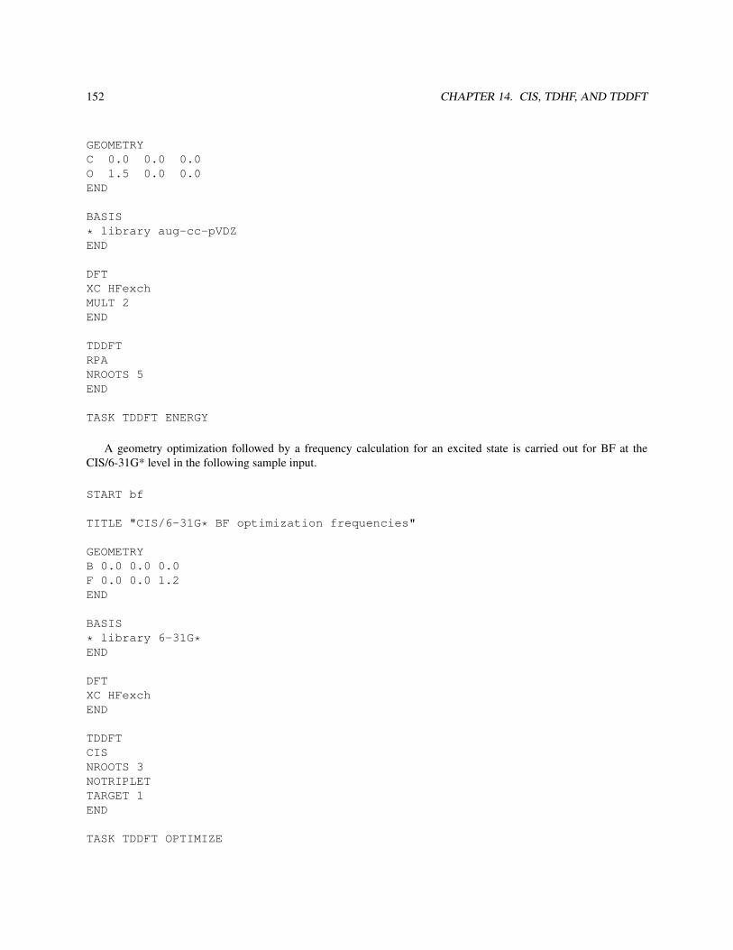
152 CHAPTER 14. CIS, TDHF, AND TDDFT
GEOMETRYC 0.0 0.0 0.0O 1.5 0.0 0.0END
BASIS
* library aug-cc-pVDZEND
DFTXC HFexchMULT 2END
TDDFTRPANROOTS 5END
TASK TDDFT ENERGY
A geometry optimization followed by a frequency calculation for an excited state is carried out for BF at theCIS/6-31G* level in the following sample input.
START bf
TITLE "CIS/6-31G* BF optimization frequencies"
GEOMETRYB 0.0 0.0 0.0F 0.0 0.0 1.2END
BASIS
* library 6-31G*END
DFTXC HFexchEND
TDDFTCISNROOTS 3NOTRIPLETTARGET 1END
TASK TDDFT OPTIMIZE

14.5. SAMPLE INPUT 153
TASK TDDFT FREQUENCIES
TDDFT with an asymptotically corrected SVWN exchange-correlation potential. Casida-Salahub scheme has beenused with the shift value of 0.1837 a.u. supplied as an input parameter.
START tddft_ac_co
GEOMETRYO 0.0 0.0 0.0000C 0.0 0.0 1.1283END
BASIS SPHERICALC library aug-cc-pVDZO library aug-cc-pVDZEND
DFTXC Slater VWN_5CS00 0.1837END
TDDFTNROOTS 12END
TASK TDDFT ENERGY
TDDFT with an asymptotically corrected B3LYP exchange-correlation potential. Hirata-Zhan-Apra-Windus-Dixon scheme has been used (this is only meaningful with B3LYP functional).
START tddft_ac_co
GEOMETRYO 0.0 0.0 0.0000C 0.0 0.0 1.1283END
BASIS SPHERICALC library aug-cc-pVDZO library aug-cc-pVDZEND
DFTXC B3LYPCS00END
TDDFTNROOTS 12END

154 CHAPTER 14. CIS, TDHF, AND TDDFT
TASK TDDFT ENERGY

Chapter 15
Tensor Contraction Engine Module: CI,MBPT, and CC
15.1 Overview
The Tensor Contraction Engine (TCE) Module of NWChem implements a variety of approximations that convergeat the exact solutions of Schrödinger equation. They include configuration interaction theory through singles, dou-bles, triples, and quadruples substitutions, coupled-cluster theory through connected singles, doubles, triples, andquadruples substitutions, and many-body perturbation theory through fourth order in its tensor formulation. Not onlyoptimized parallel programs of some of these high-end correlation theories are new, but also the way in which theyhave been developed is unique. The working equations of all of these methods have been derived completely auto-matically by a symbolic manipulation program called a Tensor Contraction Engine (TCE), and the optimized parallelprograms have also been computer-generated by the same program, which were interfaced to NWChem. The devel-opment of the TCE program and this portion of the NWChem program has been financially supported by the UnitedStates Department of Energy, Office of Science, Office of Basic Energy Science, through the SciDAC program.
The capabilities of the module include:
• Restricted Hartree–Fock, unrestricted Hartree–Fock, and restricted open-shell Hartree–Fock references,
• Restricted KS DFT and unrestricted KS DFT references,
• Unrestricted configuration interaction theory (CISD, CISDT, and CISDTQ),
• Unrestricted coupled-cluster theory (LCCD, CCD, LCCSD, CCSD, QCISD, CCSDT, CCSDTQ),
• Unrestricted iterative many-body perturbation theory [MBPT(2), MBPT(3), MBPT(4)] in its tensor formulation,
New capabilities added in the version 4.6 are:
• Unrestricted coupled-cluster singles and doubles with perturbative connected triples {CCSD(T), CCSD[T]},
• Unrestricted equation-of-motion coupled-cluster theory (EOM-CCSD, EOM-CCSDT, EOM-CCSDTQ) for ex-citation energies, transition moments and oscillator strengths, and excited-state dipole moments,
• Unrestricted coupled-cluster theory (CCSD, CCSDT, CCSDTQ) for dipole moments.
155

156 CHAPTER 15. TENSOR CONTRACTION ENGINE MODULE: CI, MBPT, AND CC
Version 4.6 and onwards the distributed binary executables do not contain CCSDTQ and its derivative methods, owingto their large volume. The source code includes them, so a user can reinstate them by setenv CCSDTQ yes andrecompile TCE module. The following optimizations have been used in the module:
• Spin symmetry (spin integration is performed wherever possible within the unrestricted framework, making thepresent unrestricted program optimal for an open-shell system. The spin adaption was not performed, althoughin a restricted calculation for a closed-shell system, certain spin blocks of integrals and amplitudes are furtheromitted by symmetry, and consequently, the present unrestricted CCSD requires only twice as many operationsas a spin-adapted restricted CCSD for a closed-shell system),
• Point-group symmetry,
• Index permutation symmetry,
• Runtime orbital range tiling for memory management,
• Dynamic load balancing (local index sort and matrix multiplications) parallelism,
• Multiple parallel I/O schemes including fully in-core algorithm using Global Arrays,
• Frozen core and virtual approximation.
• DIIS extrapolation and Jacobi update of excitation amplitudes
In addition to changes made in the 4.7 version the most essential component of the 5.0 release include:
• Several variants of active-space CCSDt and EOMCCSDt methods that employ limited set of triply excitedcluster amplitudes defined by active orbitals.
• Ground-state non-iterative CC approaches that account for the effect of triply and/or quadruply excited con-nected clusters: the perturbative approaches based on the similarity transformed Hamiltonian: CCSD(2), CCSD(2)T ,CCSDT(2)Q, the completely and locally renormalized methods: CR-CCSD(T), LR-CCSD(T), LR-CCSD(TQ)-1.
• Excited-state non-iterative corrections due to triples to the EOMCCSD excitation energies: the completelyrenormalized EOMCCSD(T) method (CR-EOMCCSD(T)).
• Improved DIIS solver.
• New form of the offset tables for files that store cluster amplitudes, recursive intermediates, and one- and two-electron integrals.
• More efficient storage of two-electron integrals for CC calculations based on the RHF or ROHF references.
• Improved scalability of the CCSD and CCSD(T) codes.
New features in the 5.1 release included:
• Dynamic dipole polarizabilities at the CCSD and CCSDT levels using the linear response formalism.
• Ground- and excited- states the iterative second-order model CC2.
• Improved algorithms for the 2-e integral transformation.
• Improvements in time-to-solution and memory use for commonly used methods.
15.2. PERFORMANCE OF CI, MBPT, AND CC METHODS 157
New features in the 5.2 release include:
• Additional algorithms for the 2-e integral transformation, including efficient and scalable spin-free out-of-coreN5 algorithms.
• Hybrid I/O schemes for both spin-orbital and spin-free calculations which eliminate the memory bottleneck ofthe 2-e integrals in favor of disk storage. Calculations with nearly 400 basis functions at the CCSD(T) can beperformed on workstation using this method.
• Parallel check-pointing and restart for ground-state (including property) calculations at the CCSD, CCSDT andCCSDTQ levels of theory.
• Dynamic dipole polarizabilities at the CCSDTQ level using the linear response formalism.
15.2 Performance of CI, MBPT, and CC methods
For reviews or tutorials of these highly-accurate correlation methods, the user is referred to:
• Trygve Helgaker, Poul JÃÿrgensen and Jeppe Olsen, Molecular Electronic-Structure Theory.
• A. Szabo and N. S. Ostlund, Modern Quantum Chemistry: Introduction to Advanced Electronic Structure The-ory.
• B. O. Roos (editor), Lecture Notes in Quantum Chemistry.
For background on development of the symbolic algebra tools which help create the code used in this model see:
• S. Hirata, J. Phys. Chem. A 107, 9887 (2003).
• S. Hirata, J. Chem. Phys. 121, 51 (2004).
• S. Hirata, Theor. Chem. Acc. 116, 2 (2006).
For details of the CC algorithms implemented in 5.0 version, see:
• S. Hirata, P.-D. Fan, A.A. Auer, M. Nooijen, P. Piecuch, J. Chem. Phys. 121, 12197 (2004).
• K. Kowalski, S. Hirata, M. Włoch, P. Piecuch, T.L. Windus, J. Chem. Phys. 123, 074319 (2005).
• K. Kowalski, P. Piecuch, J. Chem. Phys. 115, 643 (2001).
• K. Kowalski, P. Piecuch, Chem. Phys. Lett. 347, 237 (2001).
• P. Piecuch, S.A. Kucharski, and R.J. Bartlett, J. Chem. Phys. 110, 6103 (1999).
• P. Piecuch, N. Oliphant, and L. Adamowicz, J. Chem. Phys. 99, 1875 (1993).
• N. Oliphant and L. Adamowicz, Int. Rev. Phys. Chem. 12, 339 (1993).
• P. Piecuch, N. Oliphant, and L. Adamowicz, J. Chem. Phys. 99, 1875 (1993).
• K. Kowalski, P. Piecuch, J. Chem. Phys. 120, 1715 (2004).
• K. Kowalski, J. Chem. Phys. 123, 014102 (2005).

158 CHAPTER 15. TENSOR CONTRACTION ENGINE MODULE: CI, MBPT, AND CC
• P. Piecuch, K. Kowalski, I.S.O. Pimienta, M.J. McGuire, Int. Rev. Phys. Chem. 21, 527 (2002).
• K. Kowalski, P. Piecuch, J. Chem. Phys. 122, 074107 (2005)
• K. Kowalski, W. de Jong, J. Mol. Struct.: THEOCHEM, 768, 45 (2006).
and references therein.
For details of the CC methods implemented in 5.1 version, see:
• O. Christiansen, H. Koch, P. Jørgensen, Chem. Phys. Lett. 243, 409 (1995).
• K. Kowalski, J. Chem. Phys. 125, 124101 (2006)
and references therein.
15.3 Algorithms of CI, MBPT, and CC methods
15.3.1 Spin, spatial, and index permutation symmetry
The TCE thoroughly analyzes the working equation of many-electron theory models and automatically generates aprogram that takes full advantage of these symmetries at the same time. To do so, the TCE first recognizes the indexpermutation symmetries among the working equations, and perform strength reduction and factorization by carefullymonitoring the index permutation symmetries of intermediate tensors. Accordingly, every input and output tensor(such as integrals, excitation amplitudes, residuals) has just two independent but strictly ordered index strings, andeach intermediate tensor has just four independent but strictly ordered index strings. The operation cost and storagesize of tensor contraction is minimized by using the index range restriction arising from these index permutationsymmetries and also spin and spatial symmetry integration.
15.3.2 Runtime orbital range tiling
To maintain the peak local memory usage at a manageable level, in the beginning of the calculation, the orbitalsare rearranged into tiles (blocks) that contains orbitals with the same spin and spatial symmetries. So the tensorcontractions in these methods are carried out at the tile level; the spin, spatial, and index permutation symmetry isemployed to reduce the operation and storage cost at the tile level also.
15.3.3 Dynamic load balancing parallelism
In a parallel execution, dynamic load balancing of tile-level local tensor index sorting and local tensor contraction(matrix multiplication) will be invoked.
15.3.4 Parallel I/O schemes
Each process is assigned a local tensor index sorting and tensor contraction dynamically. It must first retrieve thetiles of input tensors, and perform these local operations, and accumulate the output tensors to the storage. We havedeveloped a uniform interface for these I/O operations to either (1) a global file on a global file system, (2) a globalmemory on a global or distributed memory system, and (3) semi-replicated files on a distributed file systems. Some ofthese operations depend on the ParSoft library.

15.4. INPUT SYNTAX 159
15.4 Input syntax
The keyword to invoke the many-electron theories in the module is TCE. To perform a single-point energy calculation,include
TASK TCE ENERGY
in the input file, which may be preceeded by the TCE input block that details the calculations:
TCE[(DFT||HF||SCF) default HF=SCF][FREEZE [[core] (atomic || <integer nfzc default 0>)] \
[virtual <integer nfzv default 0>]][(LCCD||CCD||CCSD||CC2||LR-CCSD||LCCSD||CCSDT||CCSDTA||CCSDTQ|| \
CCSD(T)||CCSD[T]||CCSD(2)_T||CCSD(2)||CCSDT(2)_Q|| \CR-CCSD[T]||CR-CCSD(T)|| \LR-CCSD(T)||LR-CCSD(TQ)-1||CREOMSD(T)|| \QCISD||CISD||CISDT||CISDTQ|| \MBPT2||MBPT3||MBPT4||MP2||MP3||MP4) default CCSD]
[THRESH <double thresh default 1e-6>][MAXITER <integer maxiter default 100>][PRINT (none||low||medium||high||debug)
<string list_of_names ...>][IO (fortran||eaf||ga||sf||replicated||dra||ga_eaf) default ga][DIIS <integer diis default 5>][LSHIFT <double lshift default is 0.0d0>][NROOTS <integer nroots default 0>][TARGET <integer target default 1>][TARGETSYM <character targetsym default ’none’>][SYMMETRY][2EORB][2EMET <integer fast2e default 1>][T3A_LVL][ACTIVE_OA][ACTIVE_OB][ACTIVE_VA][ACTIVE_VB][DIPOLE][TILESIZE <no default (automatically adjusted)>][(NO)FOCK <logical recompf default .true.>][FRAGMENT <default -1 (off)>][DENSMAT <filename>]
END
Also supported are energy gradient calculation, geometry optimization, and vibrational frequency (or hessian) calcu-lation, on the basis of numerical differentiation. To perform these calculations, use
TASK TCE GRADIENT
or

160 CHAPTER 15. TENSOR CONTRACTION ENGINE MODULE: CI, MBPT, AND CC
TASK TCE OPTIMIZE
or
TASK TCE FREQUENCIES
The user may also specify the parameters of reference wave function calculation in a separate block for either HF(SCF) or DFT, depending on the first keyword in the above syntax.
Since every keyword except the model has a default value, a minimal input file will be
GEOMETRYBe 0.0 0.0 0.0END
BASISBe library cc-pVDZEND
TCEccsdEND
TASK TCE ENERGY
which performs a CCSD/cc-pVDZ calculation of the Be atom in its singlet ground state with a spin-restricted HFreference.
15.5 Keywords of TCE input block
15.5.1 HF, SCF, or DFT — the reference wave function
This keyword tells the module which of the HF (SCF) or DFT module is going to be used for the calculation of areference wave function. The keyword HF and SCF are one and the same keyword internally, and are default. Whenthese are used, the details of the HF (SCF) calculation can be specified in the SCF input block, whereas if DFT ischosen, DFT input block may be provided.
For instance, RHF-RCCSDT calculation (R standing for spin-restricted) can be performed with the following inputblocks:
SCFSINGLETRHFEND
TCESCFCCSDTEND
TASK TCE ENERGY

15.5. KEYWORDS OF TCE INPUT BLOCK 161
This calculation (and any correlation calculation in the TCE module using a RHF or RDFT reference for a closed-shellsystem) skips the storage and computation of all β spin blocks of integrals and excitation amplitudes. ROHF-UCCSDT(U standing for spin-unrestricted) for an open-shell doublet system can be requested by
SCFDOUBLETROHFEND
TCESCFCCSDTEND
TASK TCE ENERGY
and likewise, UHF-UCCSDT for an open-shell doublet system can be specified with
SCFDOUBLETUHFEND
TCESCFCCSDTEND
TASK TCE ENERGY
The operation and storage costs of the last two calculations are identical. To use the KS DFT reference wave functionfor a UCCSD calculation of an open-shell doublet system,
DFTODFTMULT 2END
TCEDFTCCSDEND
TASK TCE ENERGY
Note that the default model of the DFT module is LDA.
15.5.2 CCSD,CCSDT,CCSDTQ,CISD,CISDT,CISDTQ, MBPT2,MBPT3,MBPT4, etc. — the cor-relation models
These keywords stand for the following models:

162 CHAPTER 15. TENSOR CONTRACTION ENGINE MODULE: CI, MBPT, AND CC
• LCCD: linearized coupled-cluster doubles,
• CCD: coupled-cluster doubles,
• LCCSD: linearized coupled-cluster singles & doubles,
• CCSD: coupled-cluster singles & doubles (also EOM-CCSD),
• LR-CCSD: locally renormalized EOMCCSD method,
• CC2: second-order approximate coupled cluster with singles and doubles model
• CCSDT: coupled-cluster singles, doubles, & triples (also EOM-CCSDT),
• CCSDTA: coupled-cluster singles, doubles, & active triples (also EOM-CCSDT). Three variants of the active-space CCSDt and EOMCCSDt approaches can be selected based on various definitions of triply excited clusters:(1) version I (keyword T3A_LVL 1) uses the largest set of triply excited amplitudes defined by at least oneoccupied and one unoccupied active spinorbital labels. (2) Version II (keyword T3A_LVL 2) uses triply excitedamplitudes that carry at least two occupied and unoccupied active spinorbital labels. (3) Version III (keywordT3A_LVL 3) uses triply excited amplitudes that are defined by active indices only. Each version requiresdefining relevant set of occupied active α and β spinorbitals (ACTIVE_OA and ACTIVE_OB) as well as activeunoccupied α and β spinorbitals (ACTIVE_VA and ACTIVE_VB).
• CCSDTQ: coupled-cluster singles, doubles, triples, & quadruples (also EOM-CCSDTQ),
• CCSD(T): CCSD and perturbative connected triples,
• CCSD[T]: CCSD and perturbative connected triples,
• CR-CCSD[T]: completely renormalized CCSD[T] method,
• CR-CCSD(T): completely renormalized CCSD(T) method,
• CCSD(2)_T: CCSD and perturbative CCSD(T)T correction,
• CCSD(2)_TQ: CCSD and perturbative CCSD(2) correction,
• CCSDT(2)_Q: CCSDT and perturbative CCSDT(2)Q correction.
• LR-CCSD(T): CCSD and perturbative locally renormalized CCSD(T) correction,
• LR-CCSD(TQ)-1: CCSD and perturbative locally renormalized CCSD(TQ) (LR-CCSD(TQ)-1) correction,
• CREOMSD(T): EOMCCSD energies and completely renormalized EOMCCSD(T)(IA) correction. In this op-tion NWCHEM prints two components: (1) total energy of the K-th state EK =EEOMCCSD
K +δCR−EOMCCSD(T),IAK (T )
and (2) the so-called δ-corrected EOMCCSD excitation energy ωCR−EOMCCSD(T),IAK =ωEOMCCSD
K +δCR−EOMCCSD(T),IAK (T ).
• QCISD: quadratic configuration interaction singles & doubles,
• CISD: configuration interaction singles & doubles,
• CISDT: configuration interaction singles, doubles, & triples,
• CISDTQ: configuration interaction singles, doubles, triples, & quadruples,
• MBPT2=MP2: iterative tensor second-order many-body or Møller–Plesset perturbation theory,
• MBPT3=MP3: iterative tensor third-order many-body or Møller–Plesset perturbation theory,
• MBPT4=MP4: iterative tensor fourth-order many-body or Møller–Plesset perturbation theory,

15.5. KEYWORDS OF TCE INPUT BLOCK 163
All of these models are based on spin-orbital expressions of the amplitude and energy equations, and designedprimarily for spin-unrestricted reference wave functions. However, for a restricted reference wave function of a closed-shell system, some further reduction of operation and storage cost will be made. Within the unrestricted framework,all these methods take full advantage of spin, spatial, and index permutation symmetries to save operation and storagecosts at every stage of the calculation. Consequently, these computer-generated programs will perform significantlyfaster than, for instance, a hand-written spin-adapted CCSD program in NWChem, although the nominal operationcost for a spin-adapted CCSD is just one half of that for spin-unrestricted CCSD (in spin-unrestricted CCSD there arethree independent sets of excitation amplitudes, whereas in spin-adapted CCSD there is only one set, so the nominaloperation cost for the latter is one third of that of the former. For a restricted reference wave function of a closed-shellsystem, all β spin block of the excitation amplitudes and integrals can be trivially mapped to the all α spin block,reducing the ratio to one half).
While the MBPT (MP) models implemented in the TCE module give identical correlation energies as conventionalimplementation for a canonical HF reference of a closed-shell system, the former are intrinsically more general andtheoretically robust for other less standard reference wave functions and open-shell systems. This is because the zerothorder of Hamiltonian is chosen to be the full Fock operatior (not just the diagonal part), and no further approximationwas invoked. So unlike the conventional implementation where the Fock matrix is assumed to be diagonal and acorrelation energy is evaluated in a single analytical formula that involves orbital energies (or diagonal Fock matrixelements), the present tensor MBPT requires the iterative solution of amplitude equations and subsequent energyevaluation and is generally more expensive than the former. For example, the operation cost of many conventionalimplementation of MBPT(2) scales as the fourth power of the system size, but the cost of the present tensor MBPT(2)scales as the fifth power of the system size, as the latter permits non-canonical HF reference and the former does not(to reinstate the non-canonical HF reference in the former makes it also scale as the fifth power of the system size).
15.5.3 THRESH — the convergence threshold of iterative solutions of amplitude equations
This keyword specifies the convergence threshold of iterative solutions of amplitude equations, and applies to all ofthe CI, CC, and MBPT models. The threshold refers to the norm of residual, namely, the deviation from the amplitudeequations. The default value is 1e-6.
15.5.4 MAXITER — the maximum number of iterations
It sets the maximum allowed number iterations for the iterative solutions of amplitude equations. The default value is100.
15.5.5 IO — parallel I/O scheme
There are five parallel I/O schemes implemented for all the models, which need to be wisely chosen for a particularproblem and computer architecture.
• fortran : Fortran77 direct access,
• eaf : Exclusive Access File library,
• ga : Fully incore, Global Array virtual file,
• sf : Shared File library,
• replicated : Semi-replicated file on distributed file system with EAF library.
• dra : Distributed file on distributed file system with DRA library.

164 CHAPTER 15. TENSOR CONTRACTION ENGINE MODULE: CI, MBPT, AND CC
• ga_eaf : Semi-replicated file on distributed file system with EAF library. GA is used to speedup the filereconciliation.
The GA algorithm, which is default, stores all input (integrals and excitation amplitudes), output (residuals), andintermediate tensors in the shared memory area across all nodes by virtue of GA library. This fully incore algorithmreplaces disk I/O by inter-process communications. This is a recommended algorithm whenever feasible. Note that thememory management through runtime orbital range tiling described above applies to local (unshared) memory of eachnode, which may be separately allocated from the shared memory space for GA. So when there is not enough sharedmemory space (either physically or due to software limitations, in particular, shmmax setting), the GA algorithmcan crash due to an out-of-memory error. The replicated scheme is the currently the only disk-based algorithm fora genuinely distributed file system. This means that each node keeps an identical copy of input tensors and it holdsnon-identical overlapping segments of intermediate and output tensors in its local disk. Whenever data coherency isrequired, a file reconcilation process will take place to make the intermediate and output data identical throughout thenodes. This algorithm, while requiring redundant data space on local disk, performs reasonably efficiently in parallel.For sequential execution, this reduces to the EAF scheme. For a global file system, the SF scheme is recommended.This together with the Fortran77 direct access scheme does not usually exhibit scalability unless shared files on theglobal file system also share the same I/O buffer. For sequential executions, the SF, EAF, and replicated schemes areinterchangeable, while the Fortran77 scheme is appreciably slower.
Two new I/O algorithms dra and ga_eaf combines GA and DRA or EAF based replicated algorithm. In theformer, arrays that are not active (e.g., prior T amplitudes used in DIIS or EOM-CC trial vectors) in GA algorithmwill be moved to DRA. In the latter, the intermediates that are formed by tensor contractions are initially stored inGA, thereby avoiding the need to accumulate the fragments of the intermediate scattered in EAFs in the original EAFalgorithm. Once the intermediate is formed completely, then it will be replicated as EAFs.
The spin-free 4-index transformation algorithms are exclusively compatible with the GA I/O scheme, althoughout-of-core algorithms for the 4-index transformation are accessible using the 2emet options. See 15.5.12 for details.
15.5.6 DIIS — the convergence acceleration
It sets the number iterations in which a DIIS extrapolation is performed to accelerate the convergence of excitationamplitudes. The default value is 5, which means in every five iteration, one DIIS extrapolation is performed (and inthe rest of the iterations, Jacobi rotation is used). When zero or negative value is specified, the DIIS is turned off. It isnot recommended to perform DIIS every iteration, whereas setting a large value for this parameter necessitates a largememory (disk) space to keep the excitation amplitudes of previous iterations. In 5.0 version we significantly improvedthe DIIS solver by re-organizing the itrative process and by introducing the level shift option (lshift) that enableto increase small orbital energy differences used in calculating the up-dates for cluster amplitudes. Typical valuesfor lshift oscillates between 0.3 and 0.5 for CC calculations for ground states of multi-configurational character.Otherwise, the value of lshift is by default set equal to 0.
15.5.7 FREEZE — the frozen core/virtual approximation
Some of the lowest-lying core orbitals and/or some of the highest-lying virtual orbitals may be excluded in the calcula-tions by this keyword (this does not affect the ground state HF or DFT calculation). No orbitals are frozen by default.To exclude the atom-like core regions altogether, one may request
FREEZE atomic
To specify the number of lowest-lying occupied orbitals be excluded, one may use

15.5. KEYWORDS OF TCE INPUT BLOCK 165
FREEZE 10
which causes 10 lowest-lying occupied orbitals excluded. This is equivalent to writing
FREEZE core 10
To freeze the highest virtual orbitals, use the virtual keyword. For instance, to freeze the top 5 virtuals
FREEZE virtual 5
15.5.8 NROOTS — the number of excited states
One can specify the number of excited state roots to be determined. The default value is 1. It is advised that the usersrequest several more roots than actually needed, since owing to the nature of the trial vector algorithm, some low-lyingroots can be missed when they do not have sufficient overlap with the initial guess vectors.
15.5.9 TARGET and TARGETSYM — the target root and its symmetry
At the moment, the first and second geometrical derivatives of excitation energies that are needed in force, geome-try, and frequency calculations are obtained by numerical differentiation. These keywords may be used to specifywhich excited state root is being used for the geometrical derivative calculation. For instance, when TARGET 3 andTARGETSYM a1g are included in the input block, the total energy (ground state energy plus excitation energy) ofthe third lowest excited state root (excluding the ground state) transforming as the irreducible representation a1g willbe passed to the module which performs the derivative calculations. The default values of these keywords are 1 andnone, respectively.
The keyword TARGETSYM is essential in excited state geometry optimization, since it is very common that theorder of excited states changes due to the geometry changes in the course of optimization. Without specifying theTARGETSYM, the optimizer could (and would likely) be optimizing the geometry of an excited state that is differentfrom the one the user had intended to optimize at the starting geometry. On the other hand, in the frequency calcula-tions, TARGETSYM must be none, since the finite displacements given in the course of frequency calculations willlift the spatial symmetry of the equilibrium geometry. When these finite displacements can alter the order of excitedstates including the target state, the frequency calculation is not be feasible.
15.5.10 SYMMETRY — restricting the excited state symmetry
By adding this keyword to the input block, the user can request the module to seek just the roots of the specifiedirreducible representation as TARGETSYM. By default, this option is not set. TARGETSYM must be specified whenSYMMETRY is invoked.
15.5.11 2EORB — alternative storage of two-electron integrals
In the 5.0 version a new option has been added in order to provide more economical way of storing two-electronintegrals used in CC calculations based on the RHF and ROHF references. The 2EORB keyword can be used for all CCmethods except for those using an active-space (CCSDt). All two-electron integrals are transformed and subsequentlystored in a way which is compatible with assumed tiling scheme. The transformation from orbital to spinorbital formof the two-electron integrals is performed on-the-fly during execution of the CC module. This option, although slower,

166 CHAPTER 15. TENSOR CONTRACTION ENGINE MODULE: CI, MBPT, AND CC
allows to significantly reduce the memory requirements needed by the first half of 4-index transformation and final filewith fully transformed two-electron integrals . Savings in the memory requirements on the order of magnitude (andmore) have been observed for large-scale open-shell calculations.
15.5.12 2EMET — alternative storage of two-electron integrals
In addition to the algorithm implemented in the 5.0 version, several new computation-intensive algorithms has beenadded to the 5.1 version with the purpose of improving scalability and overcoming local memory bottleneck of the 5.02EORB 4-index transformation. In order to give the user a full control over this part of the TCE code several keywordswere designed to define the most vital parameters that determine the perfromance of 4-index transformation. All newkeywords must be used with the 2EORB keyword. The 2emet keyword (default value 1 or "2emet 1", refers to the5.0 version of the 4-index transformation), defines the algorithm to be used. By putting "2emet 2" the TCE codewill execute the algoritm based on the two step procedure with two intermediate files. In some instances this algorithmis characterized by better timings compared to algorithms 3 and 4, although it is more memory demanding. In contrastto algorithms nr 1,3, and 4 this approach can make use of a disk to store intermediate files. For this purpose oneshould use the keyword idiskx ("idiskx 0" causes that all intermediate files are stored on global arrays, while"idiskx 1" tells the code to use a disk to store intermediates; default value of idiskx is equal 0). Algorithm nr3 ("2emet 3") uses only one intermediate file whereas algorithm nr 4 ("2emet 4") is a version of algorithm 3 withthe option of reducing the memory requirements. For example, by using new keyword "split 4" we will reducethe size of only intermediate file by factor of 4 (the split keyword can be only used in the context of algorithmnr 4). All new algorithms (i.e. 2emet 2+) use the attilesize setting to define the size of the atomic tile. Bydefault attilesize is set equal 30. For larger systems the use of larger values of attilesize is recommended(typically between 40-60).
Additional algorithms for version 5.2 are numbers 5, 6 and 9. Other values of 2emet are not supported and referto methods which do not function properly. Algorithms 5 and 6 were written as out-of-core N5 methods (idiskx1) and are the most efficient algorithms at the present time. The corresponding in-core variants (idiskx 0) areavailable but require excessive memory with respect to the methods discussed above, although they may be faster ifsufficient memory is available (to get enough memory often requires excessive nodes, which decreases performancein the later stages of the calculation). The difference between 5 and 6 is that 5 writes to a single file (SF or GA) while6 uses multiple files. For smaller calculations, particularly single-node jobs, 5 is faster than 6, but for more than ahandful of processors, algorithm 6 should be used. The perforance discrepancy depends on the hardware used butin algorithm eliminates simulataneous disk access on parallel file systems or memory mutexes for the in-core case.For NFS filesystems attached to parallel clusters, no performance differences have been observed, but for Lustre andPVFS they are signficant. Using algorithm 5 for large parallel file systems will make the file system inaccessible toother users, invoking the wrath of system administrators.
Algorithm 9 is an out-of-core solution to the memory bottleneck of the 2-e integrals. In this approach, the inter-mediates of the 4-index transformation as well as the MO integrals are stored in an SF file. As before, this requires ashared file system. The primary purpose of algorithm 9 is to make the performance of the NWChem coupled-clustercodes competive with fast serial codes on workstations. It does not work in parallel for all machines and thus shouldonly be used in serial. It succeeds in this purpose when corresponding functionality is compared. A more scalableversion of this algorithm is possible, but the utility is limited since large parallel computers do not permit the walltimes necessary to use an out-of-core method, which is necessarily slower than the in-core variant. An extensiblesolution to these issues using complex heterogeneous I/O is in development.
New to 5.2 is the inclusion of multiple 2emet options for the spin-orbital transformations, which are the defaultwhen 2eorb is not set and are mandatory for UHF and KS references. The are currently three algorithms 1, 2 and3 available. The numbering scheme does not correspond in any way to the numbering scheme for the 2eorb case,except that 2emet 1 corresponds to the default algorithm present in previous releases, which uses the user-definedI/O scheme. Algorithm 2 (2emet 2) writes an SF file for the half-transformed integrals, which is at least an order-of-

15.6. SAMPLE INPUT 167
magnitude larger than the fully-transformed integrals, but stores the fully-transformed integrals in core. Thus, once the4-index transformation is complete, this algorithm will perform exactly as when algorithm 1 is used. Unfortuntely, thespin-orbital 2-e fully-transformed integrals are still quite large and an algorithm corresponding to 2eorb/2emet=9is available with 2emet 3. Algorithm 3 is also limited in its scalability, but it permits relatively large UHF-basedcalculations using single workstations for patient users.
In cases where the user has access to both shared and local filesystems for parallel calculations, the permanent_dirsetting refers to the location of SF files. The file system for scratch_dir will not be used for any of the 4-indextransformation algorithms which are compatible with io=ga.
In the later part of this manual several examples illustrate the use of the newly introduced keywords.
15.5.13 DIPOLE — the ground- and excited-state dipole moments
When this is set, the ground-state CC calculation will enter another round of iterative step for the so-called Λ equationto obtain the one-particle density matrix and dipole moments. Likewise, for excited-states (EOM-CC), the transitionmoments and dipole moments will be computed when (and only when) this option is set. In the latter case, EOM-CCleft hand side solutions will be sought incurring approximately three times the computational cost of excitation energiesalone (note that the EOM-CC effective Hamiltonian is not Hermitian and has distinct left and right eigenvectors).
15.5.14 (NO)FOCK — (not) recompute Fock matrix
The default is FOCK meaning that the Fock matrix will be reconstructed (as opposed to using the orbital energiesas the diagonal part of Fock). This is essential in getting correct correlation energies with ROHF or DFT referencewave functions. However, currently, this module cannot reconstruct the Fock matrix when one-component relativisticeffects are operative. So when a user wishes to run TCE’s correlation methods with DK or other relativistic reference,NOFOCK must be set and orbital energies must be used for the Fock matrix.
15.5.15 PRINT — the verbosity
This keyword changes the level of output verbosity. One may also request some particular items in Table 15.1 printed.
15.6 Sample input
The following is a sample input for a ROHF-UCCSD energy calculation of a water radical cation.
START h2o
TITLE "ROHF-UCCSD/cc-pVTZ H2O"
CHARGE 1
GEOMETRYO 0.00000000 0.00000000 0.12982363H 0.75933475 0.00000000 -0.46621158H -0.75933475 0.00000000 -0.46621158END
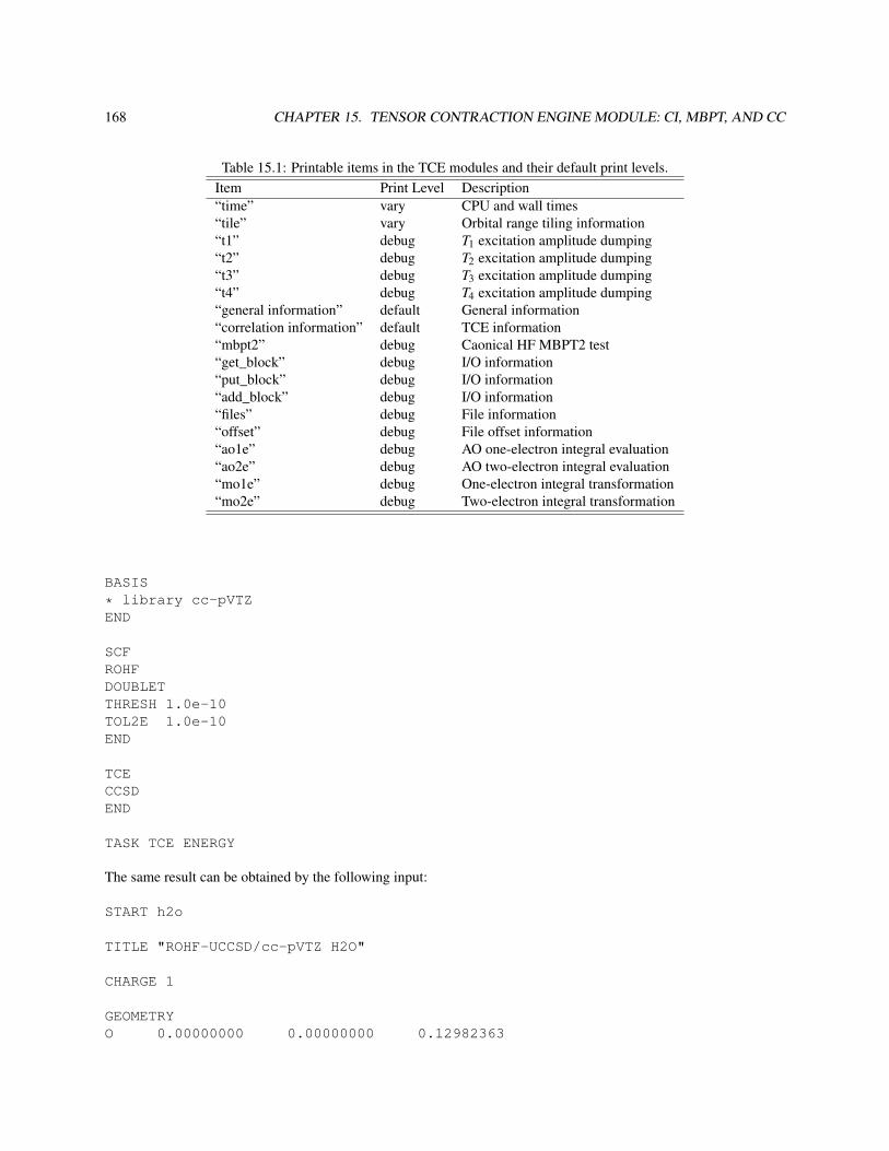
168 CHAPTER 15. TENSOR CONTRACTION ENGINE MODULE: CI, MBPT, AND CC
Table 15.1: Printable items in the TCE modules and their default print levels.Item Print Level Description“time” vary CPU and wall times“tile” vary Orbital range tiling information“t1” debug T1 excitation amplitude dumping“t2” debug T2 excitation amplitude dumping“t3” debug T3 excitation amplitude dumping“t4” debug T4 excitation amplitude dumping“general information” default General information“correlation information” default TCE information“mbpt2” debug Caonical HF MBPT2 test“get_block” debug I/O information“put_block” debug I/O information“add_block” debug I/O information“files” debug File information“offset” debug File offset information“ao1e” debug AO one-electron integral evaluation“ao2e” debug AO two-electron integral evaluation“mo1e” debug One-electron integral transformation“mo2e” debug Two-electron integral transformation
BASIS
* library cc-pVTZEND
SCFROHFDOUBLETTHRESH 1.0e-10TOL2E 1.0e-10END
TCECCSDEND
TASK TCE ENERGY
The same result can be obtained by the following input:
START h2o
TITLE "ROHF-UCCSD/cc-pVTZ H2O"
CHARGE 1
GEOMETRYO 0.00000000 0.00000000 0.12982363

15.6. SAMPLE INPUT 169
H 0.75933475 0.00000000 -0.46621158H -0.75933475 0.00000000 -0.46621158END
BASIS
* library cc-pVTZEND
SCFROHFDOUBLETTHRESH 1.0e-10TOL2E 1.0e-10END
TASK UCCSD ENERGY
EOM-CCSDT calculation for excitation energies, excited-state dipole, and transition moments.
START tce_h2o_eomcc
GEOMETRY UNITS BOHRH 1.474611052297904 0.000000000000000 0.863401706825835O 0.000000000000000 0.000000000000000 -0.215850436155089H -1.474611052297904 0.000000000000000 0.863401706825835END
BASIS
* library sto-3gEND
SCFSINGLETRHFEND
TCECCSDTDIPOLEFREEZE CORE ATOMICNROOTS 1END
TASK TCE ENERGY
Active-space CCSDt/EOMCCSDt calculations (version I) of several excited states of the Be3 molecule. Threehighest-lying occupied α and β orbitals (active_oa and active_ob) and nine lowest-lying unoccupied α and β
orbitals (active_va and active_vb) define the active space.
START TCE_ACTIVE_CCSDT

170 CHAPTER 15. TENSOR CONTRACTION ENGINE MODULE: CI, MBPT, AND CC
ECHO
GEOMETRY UNITS ANGSTROMSYMMETRY C2VBE 0.00 0.00 0.00BE 0.00 1.137090 -1.96949end
BASIS spherical# --- DEFINE YOUR BASIS SET ---END
SCFTHRESH 1.0e-10TOL2E 1.0e-10SINGLETRHFEND
TCEFREEZE ATOMICCCSDTATILESIZE 15THRESH 1.0d-5ACTIVE_OA 3ACTIVE_OB 3ACTIVE_VA 9ACTIVE_VB 9T3A_LVL 1NROOTS 2END
TASK TCE ENERGY
Completely renormalized EOMCCSD(T) (CR-EOMCCSD(T)) calculations for the ozone molecule as described bythe POL1 basis set. The CREOMSD(T) directive automatically initialize three-step procedure: (1) CCSD calculations;(2) EOMCCSD calculations; (3) non-iterative CR-EOMCCSD(T) corrections.
START TCE_CR_EOM_T_OZONE
ECHO
GEOMETRY UNITS BOHRSYMMETRY C2VO 0.0000000000 0.0000000000 0.0000000000O 0.0000000000 -2.0473224350 -1.2595211660O 0.0000000000 2.0473224350 -1.2595211660END

15.6. SAMPLE INPUT 171
BASIS SPHERICALO S
10662.285000000 0.000799001599.709700000 0.00615300364.725260000 0.03115700103.651790000 0.1155960033.905805000 0.30155200
O S12.287469000 0.444870004.756805000 0.24317200
O S1.004271000 1.00000000
O S0.300686000 1.00000000
O S0.090030000 1.00000000
O P34.856463000 0.015648007.843131000 0.098197002.306249000 0.307768000.723164000 0.49247000
O P0.214882000 1.00000000
O P0.063850000 1.00000000
O D2.306200000 0.202700000.723200000 0.57910000
O D0.214900000 0.785450000.063900000 0.53387000
END
SCFTHRESH 1.0e-10TOL2E 1.0e-10SINGLETRHFEND
TCEFREEZE ATOMICCREOMSD(T)TILESIZE 20THRESH 1.0d-6NROOTS 2END
TASK TCE ENERGY

172 CHAPTER 15. TENSOR CONTRACTION ENGINE MODULE: CI, MBPT, AND CC
The LR-CCSD(T) calculations for the glycine molecule in the aug-cc-pVTZ basis set. Option 2EORB is used inorder to minimize memory requirements associated with the storage of two-electron integrals.
START TCE_LR_CCSD_T
ECHO
GEOMETRY UNITS BOHRO -2.8770919486 1.5073755650 0.3989960497C -0.9993929716 0.2223265108 -0.0939400216C 1.6330980507 1.1263991128 -0.7236778647O -1.3167079358 -2.3304840070 -0.1955378962N 3.5887721300 -0.1900460352 0.6355723246H 1.7384347574 3.1922914768 -0.2011420479H 1.8051078216 0.9725472539 -2.8503867814H 3.3674278149 -2.0653924379 0.5211399625H 5.2887327108 0.3011058554 -0.0285088728H -3.0501350657 -2.7557071585 0.2342441831END
BASIS
* library aug-cc-pVTZEND
SCFTHRESH 1.0e-10TOL2E 1.0e-10SINGLETRHFEND
TCEFREEZE ATOMIC2EORBTILESIZE 15LR-CCSD(T)THRESH 1.0d-7END
TASK TCE ENERGY
The CCSD calculations for the triplet state of the C20 molecule. New algorithms for 4-index tranformation areused.
title "c20_cage"echostart c20_cagememory stack 2320 mb heap 180 mb global 2000 mb noverify

15.6. SAMPLE INPUT 173
geometry print xyz units bohrsymmetry c2C -0.761732 -1.112760 3.451966C 0.761732 1.112760 3.451966C 0.543308 -3.054565 2.168328C -0.543308 3.054565 2.168328C 3.190553 0.632819 2.242986C -3.190553 -0.632819 2.242986C 2.896910 -1.982251 1.260270C -2.896910 1.982251 1.260270C -0.951060 -3.770169 0.026589C 0.951060 3.770169 0.026589C 3.113776 2.128908 0.076756C -3.113776 -2.128908 0.076756C 3.012003 -2.087494 -1.347695C -3.012003 2.087494 -1.347695C 0.535910 -2.990532 -2.103427C -0.535910 2.990532 -2.103427C 3.334106 0.574125 -2.322563C -3.334106 -0.574125 -2.322563C -0.764522 -1.081362 -3.453211C 0.764522 1.081362 -3.453211
end
basis spherical
* library cc-pvtzend
scftripletrohfthresh 1.e-8maxiter 200
end
tceccsdmaxiter 60diis 5thresh 1.e-62eorb2emet 3attilesize 40tilesize 30freeze atomic
end
task tce energy

174 CHAPTER 15. TENSOR CONTRACTION ENGINE MODULE: CI, MBPT, AND CC
15.7 TCE gradients
Analytic gradients for CCSD and EOM-CCSD can be calculated for closed shell and C1 symmetry within the TCE.The input syntax to perform energy gradient calculation is
task tce gradient
One example of the input file is the following,
title waterechostart h2omemory 1500 mb
geometry units bohrO 0.000000000000 0.000000000000 -0.123909374404H 0.000000000000 1.429936611037 0.983265845431H 0.000000000000 -1.429936611037 0.983265845431symmetry c1end
basisH library sto-3gO library sto-3gend
scfthresh 1.0e-10tol2e 1.0e-10singletrhfend
tceccsdend
task tce gradient
tceccsdnroots 1end
task tce gradient

15.8. TCE RESPONSE PROPERTIES 175
15.8 TCE Response Properties
15.8.1 Introduction
Response properties can be calculated within the TCE. Ground-state dipole polarizabilities can be performed at theCCSD, CCSDT and CCSDTQ levels of theory. Neither CCSDT-LR nor CCSDTQ-LR are compiled by default. Likethe rest of the TCE, properties can be calculated with RHF, UHF, ROHF and DFT reference wavefunctions.
Specific details for the implementation of CCSD-LR and CCSDT-LR can be found in the following papers:
• J. R. Hammond, M. Valiev, W. A. deJong and K. Kowalski, J. Phys. Chem. A, 111, 5492 (2007).
• J. R. Hammond, K. Kowalski and W. A. de Jong, J. Chem. Phys., 127, 144105 (2007).
• J. R. Hammond, W. A. de Jong and K. Kowalski , J. Chem. Phys., 128, 224102 (2008).
An appropriate background on coupled-cluster linear response (CC-LR) can be found in the references of those papers.
15.8.2 Performance
The coupled-cluster response codes were generated in the same manner as the rest of the TCE, thus all previouscomments on performance apply here as well. The improved offsets available in the CCSD and EOM-CCSD codes isnow also available in the CCSD-Λ and CCSD-LR codes. The bottleneck for CCSD-LR is the same as EOM-CCSD,likewise for CCSDT-LR and EOM-CCSDT. The CCSD-LR code has been tested on as many as 1024 processors forsystems with more than 2000 spin-orbitals, while the CCSDT-LR code has been run on as many as 1024 processors.The CCSDTQ-LR code is not particularly useful due to the extreme memory requirements of quadruples amplitudes,limited scalability and poor convergence in the CCSDTQ equations in general.
15.8.3 Input
The input commands for TCE response properties exclusively use set directives (see Section 5.7) instead of TCE inputblock keywords. There are currently only three commands available:
set tce:lineresp <logical lineresp default: F>set tce:afreq <double precision afreq(9) default: 0.0>set tce:respaxis <logical respaxis(3) default: T T T>
The boolean variable lineresp invokes the linear response equations for the corresponding coupled-clustermethod (only CCSD and CCSDT possess this feature) and evaluates the dipole polarizability. When lineresp istrue, the Λ-equations will also be solved, so the dipole moment is also calculated. If no other options are set, the com-plete dipole polarizability tensor will be calculated at zero frequency (static). Up to nine real frequencies can be set;adding more should not crash the code but it will calculate meaningless quanities. If one desires to calculate more fre-quencies at one time, merely change the line double precision afreq(9) in $(NWCHEM_TOP)/src/tce/include/tce.fhappropriately and recompile.
The user can choose to calculate response amplitudes only for certain axis, either because of redundancy due tosymmetry or because of memory limitations. The boolean vector of length three respaxis is used to determinewhether or not a given set of response amplitudes are allocated, solved for, and used in the polarizability tensorevaluation. The logical variables represent the X, Y, Z axes, respectively. If respaxis is set to T F T, for example,the responses with respect to the X and Z dipoles will be calculated, and the four (three unique) tensor components

176 CHAPTER 15. TENSOR CONTRACTION ENGINE MODULE: CI, MBPT, AND CC
will be evaluated. This feature is also useful for conserving memory. By calculating only one axis at a time, memoryrequirements can be reduced by 25% or more, depending on the number of DIIS vectors used. Reducing the numberof DIIS vectors also reduces the memory requirements.
It is strongly advised that when calculating polarizabilities at high-frequencies, that user set the frequencies inincreasing order, preferably starting with zero or other small value. This approach is computationally efficient (theinitial guess for subsequent responses is the previously converged value) and mitigates starting from a zero vector forthe response amplitudes.
15.8.4 Examples
This example runs in-core on a large workstation.
geometry units angstromsymmetry d2hC 0.000 1.390 0.000H 0.000 2.470 0.000C 1.204 0.695 0.000H 2.139 1.235 0.000C 0.000 -1.390 0.000H 0.000 -2.470 0.000C -1.204 -0.695 0.000H -2.139 -1.235 0.000C 1.204 -0.695 0.000H 2.139 -1.235 0.000C -1.204 0.695 0.000H -2.139 1.235 0.000
end
basis spherical
* library aug-cc-pvdzend
tcefreeze atomicccsdio ga2eorbtilesize 16
end
set tce:lineresp Tset tce:afreq 0.000 0.072set tce:respaxis T T T
task tce energy
This is a relatively simple example for CCSDT-LR.
geometry units au

15.9. TCE RESTART CAPABILITY 177
symmetry c2vH 0 0 0F 0 0 1.7328795
end
basis spherical
* library aug-cc-pvdzend
tceccsdtio ga2eorb
end
set tce:lineresp Tset tce:afreq 0.0 0.1 0.2 0.3 0.4set tce:respaxis T F T
task tce energy
15.9 TCE Restart Capability
15.9.1 Overview
Check-pointing and restart are critical for computational chemistry applications of any scale, but particularly thosedone on supercomputers, or run for an extended period on workstations and clusters. The TCE supports parallelcheck-pointing and restart using the Shared Files (SF) library in the Global Arrays Tools. The SF library requires thatthe file system be accessible by every node, so reading and writing restart files can only be performed on a shared filesystem. For workstations, this condition is trivially met. Restart files must be persistent to be useful, so volatile filesystems or those which are periodicly erased should not be used for check-pointing.
Restart is possible for all ground-state amplitudes (T , Λ and T (1)) but not for excited-state amplitudes, as in anEOM-CC calculation. The latter functionality is under development.
Restart capability is useful in the following situations:
• The total run time is limited, as is the case for most supercomputing facilities.
• The system is volatile and jobs die randomly.
• When doing property calculations which require a large number of responses which cannot all be stored in-coresimultaneously.
At the present time, restarting the amplitudes during a potential energy surface scan or numerical geometry opt-mization/frequency calculation is not advised due to the phase issue in the molecular orbital coefficients. If the phasechanges, the amplitudes will no longer be a useful guess and may lead to nonsense results. Expert users may be ableto use restart when the geometry varies using careful choices in the SCF input by using the “rotate” and “lock” optionsbut this use of restart is not supported.
If SF encounters a failure during restart I/O, the job will fail. The capability to ignore a subset of failures, such aswhen saving the amplitudes prior to convergence, will be available in the future. This is useful on some large machines

178 CHAPTER 15. TENSOR CONTRACTION ENGINE MODULE: CI, MBPT, AND CC
when the filesystem is being taxed by another job and may be appear unavailable at the moment a check-point write isattempted.
The performance of SF I/O for restart is excellent and the wall time for reading and writing integrals and ampli-tudes is negligible, even on a supercomputer (such systems have very fast parallel file systems in most cases). Theonly platform for which restart may cause I/O problems is BlueGene, due to ratio of compute to I/O nodes (64 onBlueGene/P).
15.9.2 Input
set tce:read_integrals <logical read_integrals default: F F F F F>set tce:read_t <logical read_t default: F F F F>set tce:read_l <logical read_l default: F F F F>set tce:read_tr <logical read_tr default: F F F F>set tce:save_integrals <logical save_integrals default: F F F F F>set tce:save_t <logical save_t default: F F F F>set tce:save_l <logical save_l default: F F F F>set tce:save_tr <logical save_tr default: F F F F>set tce:save_interval <integer save_interval default: 100000>
The boolean variables read_integrals and save_integrals control which integrals are read/saved. Thefirst location is the 1-e integrals, the second is for the 2-e integrals, and the third is for dipole integrals. The fourth andfifth positions are reserved for quadrupole and octupole integrals but this functionality is not available. The read_t,read_l, read_tr, save_t, save_l and save_tr variables control the reading/saving of the T , Λ and T (1)
(response) amplitudes. Restart control on the response amplitudes is implicitly controlled by the value of respaxis(see above). Requesting amplitudes that are beyond the scope of a given calculation, such as T3 in a CCSD calculation,does not produce an error as these commands will never be processed.
Attempting to restart with a set of amplitudes without the corresponding integrals is ill-advised, due to the phaseissue discussed above. For the same reason, one cannot save a subset of the integrals, so if it is even remotelypossible that the dipole moment or polarizabilities will be desired for a given molecule, the dipole integrals shouldbe saved as well. It is possible to save the dipole integrals without setting dipole in the TCE input block; settingsave_integrals(3) true is sufficient for this to occur.
The save_interval variable controls the frequency with which amplitudes are saved. By default, the ampli-tudes are saved only when the iterative process has converged, meaning that if the iterations do not converge in lessthan the maximum, one must start the calculation again from scratch. The solution is to set save_interval to asmaller value, such as the number of DIIS cycles being used.
The user shall not change the tilesize when reading in saved amplitudes. The results of this are catastrophic andunder no circumstance will this lead to physically meaningful results.
15.9.3 Examples
geometry units ausymmetry c2vH 0 0 0F 0 0 1.7328795
end
basis spherical

15.10. MAXIMIZING PERFORMANCE 179
* library aug-cc-pvdzend
tceccsdtio ga
end
set tce:lineresp Tset tce:afreq 0.0 0.1 0.2 0.3 0.4set tce:respaxis T F T
task tce energy
15.10 Maximizing performance
The following are recommended parameters for getting the best performance and efficiency for common methods onvarious hardware configurations. The optimal settings are far from extensible and it is extremely important that userstake care in how they apply these recommendations. Testing a variety of settings on a simple example is recommendedwhen optimal settings are desired. Nonetheless, a few guiding principles will improve the performance of TCE jobsmarkedly, including making otherwise impossible jobs possible.
15.10.1 Memory considerations and IO schemes
15.10.2 Processor count
15.10.3 SCF options
15.10.4 Convergence criteria
15.10.5 Integral storage, transformation algorithms and tilesizes

180 CHAPTER 15. TENSOR CONTRACTION ENGINE MODULE: CI, MBPT, AND CC

Chapter 16
MP2
There are (at least) three algorithms within NWChem that compute the Møller-Plesset (or many-body) perturbationtheory second-order correction to the Hartree-Fock energy (MP2). They vary in capability, the size of system that canbe treated and use of other approximations
• Semi-direct — this is recommended for most large applications (up to about 2800 basis functions), especiallyon the IBM SP and other machines with significant disk I/O capability. Partially transformed integrals are storedon disk, multi-passing as necessary. RHF and UHF references may be treated including computation of analyticderivatives. This is selected by specifying mp2 on the task directive, e.g.
TASK MP2
• Fully-direct — this is of utility if only limited I/O resources are available (up to about 2800 functions). OnlyRHF references and energies are available. This is selected by specifying direct_mp2 on the task directive,e.g.
TASK DIRECT_MP2
• Resolution of the identity (RI) approximation MP2 (RI-MP2) — this uses the RI approximation and is thereforeonly exact in the limit of a complete fitting basis. However, with some care, high accuracy may be obtained withrelatively modest fitting basis sets. An RI-MP2 calculation can cost over 40 times less than the correspondingexact MP2 calculation. RHF and UHF references with only energies are available. This is selected by specifyingrimp2 on the task directive, e.g.,
TASK RIMP2
All three MP2 tasks share the same input block.
MP2[FREEZE [[core] (atomic || <integer nfzc default 0>)] \
[virtual <integer nfzv default 0>]][TIGHT][PRINT][NOPRINT][VECTORS <string filename default scf-output-vectors> \
[swap [(alpha||beta)] <integer pair-list>] ]
181

182 CHAPTER 16. MP2
[RIAPPROX <string riapprox default V>][FILE3C <string filename default $file_prefix$.mo3cint">][SCRATCHDISK <integer>]
END
16.1 FREEZE — Freezing orbitals
All MP2 modules support frozen core orbitals, however, only the direct MP2 and RI-MP2 modules support frozenvirtual orbitals.
By default, no orbitals are frozen. The atomic keyword causes orbitals to be frozen according to the rules inTable 16.1. Note that no orbitals are frozen on atoms on which the nuclear charge has been modified either by the useror due to the presence of an ECP. The actual input would be
freeze atomic
For example, in a calculation on Si(OH)2, by default the lowest seven orbitals would be frozen (the oxygen 1s, andthe silicon 1s, 2s and 2p).
Period Elements Core Orbitals Number of Core0 H – He — 01 Li – Ne 1s 12 Na – Ar 1s2s2p 53 K – Kr 1s2s2p3s3p 94 Rb – Xe 1s2s2p3s3p4s3d4p 185 Cs – Rn 1s2s2p3s3p4s3d4p5s4d5p 276 Fr – Lr 1s2s2p3s3p4s3d4p5s4d5p6s4 f 5d6p 43
Table 16.1: Number of orbitals considered “core” in the “freeze by atoms” algorithm.
Caution: The rule for freezing orbitals “by atoms” are rather unsophisticated: the number of orbitals to be frozenis computed from the Table 16.1 by summing the number of core orbitals in each atom present. The correspondingnumber of lowest-energy orbitals are frozen — if for some reason the actual core orbitals are not the lowest lying, thencorrect results will not be obtained. From limited experience, it seems that special attention should be paid to systemsincluding third- and higher- period atoms.
The user may also specify the number of orbitals to be frozen by atom. Following the Si(OH)2 example, the usercould specify
freeze atomic O 1 Si 3
In this case only the lowest four orbitals would be frozen. If the user does not specify the orbitals by atom, the rulesdefault to Table 16.1.
Caution: The system does not check for a valid number of orbitals per atom. If the user specifies to freeze moreorbitals then are available for the atom, the system will not catch the error. The user must specify a logical number oforbitals to be frozen for the atom.
The FREEZE directive may also be used to specify the number of core orbitals to freeze. For instance, to freezethe first 10 orbitals
freeze 10

16.2. TIGHT — INCREASED PRECISION 183
or equivalently, using the optional keyword core
freeze core 10
Again, note that if the 10 orbitals to be frozen do not correspond to the first 10 orbitals, then the swap keyword of theVECTORS directive must be used to order the input orbitals correctly (Section 16.5).
To freeze the highest virtual orbitals, use the virtual keyword. For instance, to freeze the top 5 virtuals
freeze virtual 5
Again, note that this only works for the direct-MP2 and RI-MP2 energy codes.
16.2 TIGHT — Increased precision
The TIGHT directive can be used to increase the precision in the MP2 energy and gradients.
By default the MP2 gradient package should compute energies accurate to better than a micro-Hartree, and gra-dients accurate to about five decimal places (atomic units). However, if there is significant linear dependence in thebasis set the precision might not be this good. Also, for computing very accurate geometries or numerical frequencies,greater precision may be desirable.
This option increases the precision to which both the SCF (from 10−6 to 10−8) and CPHF (from 10−4 to 10−6)are solved, and also tightens thresholds for computation of the AO and MO integrals (from 10−9 to 10−11) within theMP2 code.
16.3 SCRATCHDISK — Limiting I/O usage
This directive – used only in the semi-direct algorithm – allows to limit the per process disk usage. Mandatoryargument for this keyword is the maximum number of MBytes. For example, the following input line
scratchdisk 512
puts an upper limit of 512 MBytes to the semi-direct MP2 usage of disk (again, on a per process base).
16.4 PRINT and NOPRINT
The standard print control options are recognized. The list of recognized names are given in Table 16.2.
16.5 VECTORS — MO vectors
All of the (supported) MP2 modules require use of converged canonical SCF (RHF or UHF) orbitals for correct results.The vectors are by default obtained from the preceding SCF calculation, but it is possible to specify a different sourceusing the VECTORS directive. For instance, to obtain vectors from the file /tmp/h2o.movecs, use the directive
vectors /tmp/h2o.movecs

184 CHAPTER 16. MP2
Table 16.2: Printable items in the MP2 modules and their default print levels.Item Print Level Description
RI-MP2
“2/3 ints” debug Partial 3-center integrals“3c ints” debug MO 3-center integrals“4c ints b” debug “B” matrix with approx. 4c integrals“4c ints” debug Approximate 4-center integrals“amplitudes” debug “B” matrix with denominators“basis” high“fit xf” debug Transformation for fitting basis“geombas” debug Detailed basis map info“geometry” high“information” low General information about calc.“integral i/o” high File size information“mo ints” debug“pair energies” debug (working only in direct_mp2)“partial pair energies” debug Pair energy matrix each time it is updated“progress reports” default Report completion of time-consuming steps“reference” high Details about reference wavefunction“warnings” low Non-fatal warnings
As noted above (Section 16.1) if the SCF orbitals are not in the correct order, it is necessary to permute theinput orbitals using the swap keyword of the VECTORS directive. For instance, if it is desired to freeze a total sixorbitals corresponding to the SCF orbitals 1–5, and 7, it is necessary to swap orbital 7 into the 6th position. This isaccomplished by
vectors swap 6 7
The swap capability is examined in more detail in Section 10.5.
16.6 RI-MP2 fitting basis
The RI-MP2 method requires a fitting basis, which must be specified with the name "ri-mp2 basis" (see Section7). For instance,
basis "ri-mp2 basis"O s; 10000.0 1O s; 1000.0 1O s; 100.0 1...
end
Alternatively, using a standard capability of basis sets (Section 7) another named basis may be associated with thefitting basis. For instance, the following input specifies a basis with the name "small fitting basis" and thendefines this to be the "ri-mp2 basis".

16.7. FILE3C — RI-MP2 3-CENTER INTEGRAL FILENAME 185
basis "small fitting basis"H s; 10 1H s; 3 1H s; 1 1H s; 0.1 1H s; 0.01 1
end
set "ri-mp2 basis" "small fitting basis"
16.7 FILE3C — RI-MP2 3-center integral filename
The default name for the file used to store the transformed 3-center integrals is "$file_prefix$.mo3cint"in the scratch directory. This may be overridden using the FILE3C directive. For instance, to specify the file/scratch/h2o.3c, use this directive
file3c /scratch/h2o.3c
16.8 RIAPPROX — RI-MP2 Approximation
The type of RI approximation used in the RI-MP2 calculation is controlled by means of the RIAPPROX directive.The two possible values are V and SVS (case sensitive), which correspond to the approximations with the same namesdescribed in O. Vahtras, J Almlöf, and M. W. Feyereisen, Chem. Phys. Lett. 213, 514–518 (1993). The default is V.
16.9 Advanced options for RI-MP2
These options, which functioned at the time of writing, are not currently supported.
16.9.1 Control of linear dependence
Construction of the RI fit requires the inversion of a matrix of fitting basis integrals which is carried out via diago-nalization. If the fitting basis includes near linear dependencies, there will be small eigenvalues which can ultimatelylead to non-physical RI-MP2 correlation energies. Eigenvectors of the fitting matrix are discarded if the correspond-ing eigenvalue is less than $mineval$ which defaults to 10−8. This parameter may be changed by setting the aparameter in the database. For instance, to set it to 10−10
set "mp2:fit min eval" 1e-10
16.9.2 Reference Spin Mapping for RI-MP2 Calculations
The user has the option of specifying that the RI-MP2 calculations are to be done with variations of the SCF referencewavefunction. This is accomplished with a SET directive of the form,
set "mp2:reference spin mapping" <integer array default 0>

186 CHAPTER 16. MP2
Each element specified for array is the SCF spin case to be used for the corresponding spin case of the correlatedcalculation. The number of elements set determines the overall type of correlated calculation to be performed. Thedefault is to use the unadulterated SCF reference wavefunction.
For example, to perform a spin-unrestricted calculation (two elements) using the alpha spin orbitals (spin case 1)from the reference for both of the correlated reference spin cases, the SET directive would be as follows,
set "mp2:reference spin mapping" 1 1
The SCF calculation to produce the reference wavefunction could be either RHF or UHF in this case.
The SET directive for a similar case, but this time using the beta-spin SCF orbitals for both correlated spin cases,is as follows,
set "mp2:reference spin mapping" 2 2
The SCF reference calculation must be UHF in this case.
The SET directive for a spin-restricted calculation (one element) from the beta-spin SCF orbitals using this optionis as follows,
set "mp2:reference spin mapping" 2
The SET directive for a spin-unrestricted calculation with the spins flipped from the original SCF reference wave-function is as follows,
set "mp2:reference spin mapping" 2 1
16.9.3 Batch Sizes for the RI-MP2 Calculation
The user can control the size of each batch in the transformation and energy evaluation in the MP2 calculation, andconsequently the memory requirements and number of passes required. This is done using two SET directives of thefollowing form,
set "mp2:transformation batch size" <integer size default -1>set "mp2:energy batch size" <integer isize jsize default -1 -1>
The default is for the code to determine the batch size based on the available memory. Should there be problemswith the program-determined batch sizes, these variables allow the user to override them. The program will alwaysuse the smaller of the user’s value of these entries and the internally computed batch size.
The transformation batch size computed in the code is the number of occupied orbitals in the (occ vir| f it) three-center integrals to be produced at a time. If this entry is less than the number of occupied orbitals in the system, thetransformation will require multiple passes through the two-electron integrals. The memory requirements of this stageare two global arrays of dimension < batchsize >×vir× f it with the “fit” dimension distributed across all processors(on shell-block boundaries). The compromise here is memory space versus multiple integral evaluations.
The energy evaluation batch sizes are computed in the code from the number of occupied orbitals in the two sets ofthree-center integrals to be multiplied together to produce a matrix of approximate four-center integrals. Two blocksof integrals of dimension (< batchisize >×vir) and (< batch jsize >×vir) by fit are read in from disk and multipliedtogether to produce < batchisize >< batch jsize > vir2 approximate integrals. The compromise here is performanceof the distributed matrix multiplication (which requires large matrices) versus memory space.
16.10. ONE-ELECTRON PROPERTIES AND NATURAL ORBITALS 187
16.9.4 Energy Memory Allocation Mode: RI-MP2 Calculation
The user must choose a strategy for the memory allocation in the energy evaluation phase of the RI-MP2 calculation,either by minimizing the amount of I/O, or minimizing the amount of computation. This can be accomplished using aSET directive of the form,
set "mp2:energy mem minimize" <string mem_opt default I>
A value of I entered for the string mem_opt means that a strategy to minimize I/O will be employed. A value ofC tells the code to use a strategy that minimizes computation.
When the option to minimize I/O is selected, the block sizes are made as large as possible so that the total numberof passes through the integral files is as small as possible. When the option to minimize computation is selected, theblocks are chosen as close to square as possible so that permutational symmetry in the energy evaluation can be usedmost effectively.
16.9.5 Local Memory Usage in Three-Center Transformation
For most applications, the code will be able to size the blocks without help from the user. Therefore, it is unlikelythat users will have any reason to specify values for these entries except when doing very particular performancemeasurements.
The size of xf3ci:AO 1 batch size is the most important of the three, in terms of the effect on performance.
Local memory usage in the first two steps of the transformation is controlled in the RI-MP2 calculation using thefollowing SET directives,
set "xf3ci:AO 1 batch size" <integer max>set "xf3ci:AO 2 batch size" <integer max>set "xf3ci:fit batch size" <integer max>
The size of the local arrays determines the sizes of the two matrix multiplications. These entries set limits on thesize of blocks to be used in each index. The listing above is in order of importance of the parameters to performance,with xf3ci:AO 1 batch size being most important.
Note that these entries are only upper bounds and that the program will size the blocks according to what itdetermines as the best usage of the available local memory. The absolute maximum for a block size is the number offunctions in the AO basis, or the number of fitting basis functions on a node. The absolute minimum value for blocksize is the size of the largest shell in the appropriate basis. Batch size entries specified for max that are larger thanthese limits are automatically reset to an appropriate value.
16.10 One-electron properties and natural orbitals
If an MP2 energy gradient is computed, all contributions are available to form the MP2 linear-response density. Thisis the density that when contracted with any spin-free, one-electron operator yields the associated property defined asthe derivative of the energy. Thus, the reported MP2 dipole moment is the derivative of the energy w.r.t. an externalmagnetic field and is not the expectation value of the operator over the wavefunction. Only dipole moments are printedby the MP2 gradient code, but natural orbitals are produced and stored in the permanent directory with a file extensionof ".mp2nos". These may be fed into the property package (see Section 30) to compute more general properties.

188 CHAPTER 16. MP2
Note that the MP2 linear response density matrix is not necessarily positive definite so it is not unusual to see a fewsmall negative natural orbital occupation numbers.

Chapter 17
Multiconfiguration SCF
The NWChem multiconfiguration SCF (MCSCF) module can currently perform complete active space SCF (CASSCF)calculations with at most 20 active orbitals and about 500 basis functions. It is planned to extend it to handle 1000+basis functions.
MCSCFSTATE <string state>ACTIVE <integer nactive>ACTELEC <integer nactelec>MULTIPLICITY <integer multiplicity>[SYMMETRY <integer symmetry default 1>][VECTORS [[input] <string input_file default $file_prefix$.movecs>]
[swap <integer vec1 vec2> ...] \[output <string output_file default input_file>] \[lock]
[HESSIAN (exact||onel)][MAXITER <integer maxiter default 20>][THRESH <real thresh default 1.0e-4>][TOL2E <real tol2e default 1.0e-9>][LEVEL <real shift default 0.1d0>]
END
Note that the ACTIVE, ACTELEC, and MULTIPLICITY directives are required. The symmetry and multiplicity mayalternatively be entered using the STATE directive.
17.1 ACTIVE — Number of active orbitals
The number of orbitals in the CASSCF active space must be specified using the ACTIVE directive.
E.g.,
active 10
The input molecular orbitals (see the vectors directive, Sections 17.6 and 10.5) must be arranged in order
189

190 CHAPTER 17. MULTICONFIGURATION SCF
1. doubly occupied orbitals,
2. active orbitals, and
3. unoccupied orbitals.
17.2 ACTELEC — Number of active electrons
The number of electrons in the CASSCF active space must be specified using the the ACTELEC directive. An error isreported if the number of active electrons and the multiplicity are inconsistent.
The number of closed shells is determined by subtracting the number of active electrons from the total number ofelectrons (which in turn is derived from the sum of the nuclear charges minus the total system charge).
17.3 MULTIPLICITY
The spin multiplicity must be specified and is enforced by projection of the determinant wavefunction.
E.g., to obtain a triplet state
multiplicity 3
17.4 SYMMETRY — Spatial symmetry of the wavefunction
This species the irreducible representation of the wavefunction as an integer in the range 1—8 using the same num-bering of representations as output by the SCF program. Note that only Abelian point groups are supported.
E.g., to specify a B1 state when using the C2v group
symmetry 3
17.5 STATE — Symmetry and multiplicity
The electronic state (spatial symmetry and multiplicity) may alternatively be specified using the conventional notationfor an electronic state, such as 3B2 for a triplet state of B2 symmetry. This would be accomplished with the input
state 3b2
which is equivalent to
symmetry 4multiplicity 3

17.6. VECTORS — INPUT/OUTPUT OF MO VECTORS 191
17.6 VECTORS — Input/output of MO vectors
Calculations are best started from RHF/ROHF molecular orbitals (see Section 10), and by default vectors are takenfrom the previous MCSCF or SCF calculation. To specify another input file use the VECTORS directive. Vectorsare by default output to the input file, and may be redirected using the output keyword. The swap keyword of theVECTORS directive may be used to reorder orbitals to obtain the correct active space. See Section 10.5 for an example.
The LOCK keyword allows the user to specify that the ordering of orbitals will be locked to that of the initial vectors,insofar as possible. The default is to order by ascending orbital energies within each orbital space. One applicationwhere locking might be desirable is a calculation where it is necessary to preserve the ordering of a previous geometry,despite flipping of the orbital energies. For such a case, the LOCK directive can be used to prevent the SCF calculationfrom changing the ordering, even if the orbital energies change.
Output orbitals of a converged MCSCF calculation are canonicalized as follows:
• Doubly occupied and unoccupied orbitals diagonalize the corresponding blocks of an effective Fock operator.Note that in the case of degenerate orbital energies this does not fully determine the orbtials.
• Active-space orbitals are chosen as natural orbitals by diagonalization of the active space 1-particle densitymatrix. Note that in the case of degenerate occupations that this does not fully determine the orbitals.
17.7 HESSIAN — Select preconditioner
The MCSCF will use a one-electron approximation to the orbital-orbital Hessian until some degree of convergenceis obtained, whereupon it will attempt to use the exact orbital-orbital Hessian which makes the micro iterations moreexpensive but potentially reduces the total number of macro iterations. Either choice may be forced throughout thecalculation by specifying the appropriate keyword on the HESSIAN directive.
E.g., to specify the one-electron approximation throughout
hessian onel
17.8 LEVEL — Level shift for convergence
The Hessian (Section 17.7) used in the MCSCF optimization is by default level shifted by 0.1 until the orbital gradientnorm falls below 0.01, at which point the level shift is reduced to zero. The initial value of 0.1 may be changed usingthe LEVEL directive. Increasing the level shift may make convergence more stable in some instances.
E.g., to set the initial level shift to 0.5
level 0.5
17.9 PRINT and NOPRINT
Specific output items can be selectively enabled or disabled using the print control mechanism (5.6) with the avail-able print options listed in table(17.9).

192 CHAPTER 17. MULTICONFIGURATION SCF
Option Class Synopsisci energy default CI energy eigenvaluefock energy default Energy derived from Fock matricesgradient norm default Gradient normmovecs default Converged occupied MO vectorstrace energy high Trace Energyconverge info high Convergence data and monitoringprecondition high Orbital preconditioner iterationsmicroci high CI iterations in line searchcanonical high Canonicalization informationnew movecs debug MO vectors at each macro-iterationci guess debug Initial guess CI vectordensity matrix debug One- and Two-particle density matrices
Table 17.1: MCSCF Print Options

Chapter 18
Selected CI
The selected CI module is integrated into NWChem but as yet no input module has been written. The input thusconsists of setting the appropriate variables in the database.
It is assumed that an initial SCF/MCSCF calculation has completed, and that MO vectors are available. These willbe used to perform a four-index transformation, if this has not already been performed.
18.1 Background
This is a general spin-adapted, configuration-driven CI program which can perform arbitrary CI calculations, the onlyrestriction being that all spin functions are present for each orbital occupation. CI wavefunctions may be specifiedusing a simple configuration generation program, but the prime usage is intended to be in combination with pertur-bation correction and selection of new configurations. The second-order correction (Epstein-Nesbet) to the CI energymay be computed, and at the same time configurations that interact greater than a certain threshold with the currentCI wavefunction may be chosen for inclusion in subsequent calculations. By repeating this process (typically twice isadequate) with the same threshold until no new configurations are added, the CI expansion may be made consistentwith the selection threshold, enabling tentative extrapolation to the full-CI limit.
A typical sequence of calculations is as follows:
1. Pick as an initial CI reference the previously executed SCF/MCSCF.
2. Define an initial selection threshold.
3. Determine the roots of interest in the current reference space.
4. Compute the perturbation correction and select additional configurations that interact greater than the currentthreshold.
5. Repeat steps 3 and 4.
6. Lower the threshold (a factor of 10 is common) and repeat steps 3, 4, and 5. The first pass through step 4 willyield the approximately self-consistent CI and CI+PT energies from the previous selection threshold.
To illustrate this, below is some abbreviated output from a calculation on water in an augmented cc-PVDZ basisset with one frozen core orbital. The SCF was converged to high precision in C2v symmetry with the following input
193

194 CHAPTER 18. SELECTED CI
start h2ogeometry; symmetry c2v
O 0 0 0; H 0 1.43042809 -1.10715266endbasis
H library aug-cc-pvdz; O library aug-cc-pvdzendtask scfscf; thresh 1d-8; end
The following input restarts from the SCF to perform a sequence of selected CI calculations with the specifiedtolerances, starting with the SCF reference.
restart h2oset fourindex:occ_frozen 1set selci:mode selectset "selci:selection thresholds" \
0.001 0.001 0.0001 0.0001 0.00001 0.00001 0.000001task selci
Table 18.1 summarizes the output from each of the major computational steps that were performed.
CIStep Description dimension Energy
1 Four-index, one frozen-core2 Config. generator, SCF default 1
3+4 CI diagonalization 1 ECI =−76.0419835 PT selection T=0.001 1 ECI+PT =−76.304797
6+7 CI diagonalization 75 ECI =−76.1108948 PT selection T=0.001 75 ECI+PT =−76.277912
9+10 CI diagonalization 75 ECI(T = 0.001) =−76.11089411 PT selection T=0.0001 75 ECI+PT (T = 0.001) =−76.277912
12+13 CI diagonalization 823 ECI =−76.22841914 PT selection T=0.0001 823 ECI+PT =−76.273751
15+16 CI diagonalization 841 ECI(T = 0.0001) =−76.230054417 PT selection T=0.00001 841 ECI+PT (T = 0.0001) =−76.274073
18+19 CI diagonalization 2180 ECI =−76.25928520 PT selection T=0.00001 2180 ECI+PT =−76.276418
21+22 CI diagonalization 2235 ECI(T = 0.00001) =−76.25981823 PT selection T=0.000001 2235 ECI+PT (T = 0.00001) =−76.27647824 CI diagonalization 11489
Table 18.1: Summary of steps performed in a selected CI calculation on water.
18.2 Files
Currently, no direct control is provided over filenames. All files are prefixed with the standard file-prefix, and any filesgenerated by all nodes are also postfixed with the processor number. Thus, for example the molecular integrals file,

18.3. CONFIGURATION GENERATION 195
used only by process zero, might be called h2o.moints whereas the off-diagonal Hamiltonian matrix element fileused by process number eight would be called h2o.hamil.8.
ciconf — the CI configuration file, which holds information about the current CI expansion, indexing vectors, etc.This is the most important file and is required for all restarts. Note that the CI configuration generator is onlyrun if this file does not exist. Referenced only by process zero.
moints— the molecular integrals, generated by the four-index transformation. As noted above these must currentlybe manually deleted, or the database entry selci:moints:force set, to force regeneration. Referencedonly by process zero.
civecs — the CI vectors. Referenced only by process zero.
wmatrx— temporary file used to hold coupling coefficients. Deleted at calculation end. Referenced only by processzero.
rtname, roname — restart information for the PT selection. Should be automatically deleted if no restart isnecessary. Referenced only by process zero.
hamdg — diagonal elements of the Hamiltonian. Deleted at calculation end. Referenced only by process zero.
hamil — off-diagonal Hamiltonian matrix elements. All processes generate a file containing a subset of theseelements. These files can become very large. Deleted at calculation end.
18.3 Configuration Generation
If no configuration is explicitly specified then the previous SCF/MCSCF wavefunction is used, adjusting for anyorbitals frozen in the four-index transformation. The four-index transformation must have completed successfullybefore this can execute. Orbital configurations for use as reference functions may also be explicitly specified.
Once the default/user-input reference configurations have been determined additional reference functions may begenerated by applying multiple sets of creation-annihilation operators, permitting for instance, the ready specificationof complete or restricted active spaces.
Finally, a uniform level of excitation from the current set of configurations into all orbitals may be applied, en-abling, for instance, the simple creation of single or single+double excitation spaces from an MCSCF reference.
18.3.1 Specifying the reference occupation
A single orbital configuration or occupation is specified by
ns (socc(i),i=1,ns) (docc(i),i=1,nd)
where ns specifies the number of singly occupied orbitals, socc() is the list of singly occupied orbitals, and docc()is the list of doubly occupied orbitals (the number of doubly occupied orbitals, nd, is inferred from ns and the totalnumber of electrons). All occupations may be strung together and inserted into the database as a single integer arraywith name "selci:conf". For example, the input
set "selci:conf" \0 1 2 3 4 \0 1 2 3 27 \

196 CHAPTER 18. SELECTED CI
0 1 3 4 19 \2 11 19 1 3 4 \2 8 27 1 2 3 \0 1 2 4 25 \4 3 4 25 27 1 2 \4 2 3 19 20 1 4 \4 2 4 20 23 1 3
specifies the following nine orbital configurations
1(2) 2(2) 3(2) 4(2)1(2) 2(2) 3(2) 27(2)1(2) 3(2) 4(2) 19(2)1(2) 3(2) 4(2) 11(1) 19(1)1(2) 2(2) 3(2) 8(1) 27(1)1(2) 2(2) 4(2) 25(2)1(2) 2(2) 3(1) 4(1) 25(1) 27(1)1(2) 2(1) 3(1) 4(2) 19(1) 20(1)1(2) 2(1) 3(2) 4(1) 20(1) 23(1)
The optional formatting of the input is just to make this arcane notation easier to read. Relatively few configurationscan be currently specified in this fashion because of the input line limit of 1024 characters.
18.3.2 Applying creation-annihilation operators
Up to 10 sets of creation-annihilation operator pairs may be specified, each set containing up to 255 pairs. This sufficesto specify complete active spaces with up to ten electrons.
The number of sets is specified as follows,
set selci:ngen 4
which indicates that there will be four sets. Each set is then specified as a separate integer array
set "selci:refgen 1" 5 4 6 4 5 3 6 3set "selci:refgen 2" 5 4 6 4 5 3 6 3set "selci:refgen 3" 5 4 6 4 5 3 6 3set "selci:refgen 4" 5 4 6 4 5 3 6 3
In the absence of friendly, input note that the names "selci:refgen n" must be formatted with n in I2 format.Each set specifies a list of creation-annihilation operator pairs (in that order). So for instance, in the above exampleeach set is the same and causes the excitations
4->5 4->6 3->5 3->6
If orbitals 3 and 4 were initially doubly occupied, and orbitals 5 and 6 initially unoccupied, then the application of thisset of operators four times in succession is sufficient to generate the four electron in four orbital complete active space.
The precise sequence in which operators are applied is
1. loop through sets of operators

18.4. NUMBER OF ROOTS 197
2. loop through reference configurations
3. loop through operators in the set
4. apply the operator to the configuration, if the result is new add it to the new list
5. end the loop over operators
6. end the loop over reference configurations
7. augment the configuration list with the new list
8. end the loop over sets of operators
18.3.3 Uniform excitation level
By default no excitation is applied to the reference configurations. If, for instance, you wanted to generate a singleexcitation CI space from the current configuration list, specify
set selci:exci 1
Any excitation level may be applied, but since the list of configurations is explicitly generated, as is the CI Hamiltonianmatrix, you will run out of disk space if you attempt to use more than a few tens of thousands of configurations.
18.4 Number of roots
By default, only one root is generated in the CI diagonalization or perturbation selection. The following requests that2 roots be generated
set selci:nroot 2
There is no imposed upper limit. If many roots are required, then, to minimize root skipping problems, it helps toperform an initial approximate diagonalization with several more roots than required, and then resetting this parameteronce satisfied that the desired states are obtained.
18.5 Accuracy of diagonalization
By default, the CI wavefunctions are converged to a residual norm of 10−6 which provides similar accuracy in theperturbation corrections to the energy, and much higher accuracy in the CI eigenvalues. This may be adjusted with
set "selci:diag tol" 1d-3
the example setting much lower precision, appropriate for the approximate diagonalization discussed in the precedingsection.

198 CHAPTER 18. SELECTED CI
18.6 Selection thresholds
When running in the selected-CI mode the program will loop through a list of selection thresholds (T ), performing theCI diagonalization, computing the perturbation correction, and augmenting the CI expansion with configurations thatmake an energy lowering to any root greater than T . The list of selection thresholds is specified as follows
set "selci:selection thresholds" \0.001 0.001 0.0001 0.0001 0.00001 0.00001 0.000001
There is no default for this parameter.
18.7 Mode
By default the program runs in "ci+davids" mode and just determines the CI eigenvectors/values in the currentconfiguration space. To perform a selected-CI with perturbation correction use the following
set selci:mode select
and remember to define the selection thresholds.
18.8 Memory requirements
No global arrays are used inside the selected-CI, though the four-index transformation can be automatically invokedand it does use GAs. The selected CI replicates inside each process
• all unique two-electron integrals in the MO basis that are non-zero by symmetry, and
• all CI information, including the CI vectors.
These large data structures are allocated on the local stack. A fatal error will result if insufficient memory is available.
18.9 Forcing regeneration of the MO integrals
When scanning a potential energy surface or optimizing a geometry the MO integrals need to be regenerated eachtime. Specify
set selci:moints:force logical .true.
to accomplish this.
18.10 Disabling update of the configuration list
When computing CI+PT energy the reference configuration list is normally updated to reflect all configurations thatinteract more than the specified threshold. This is usually desirable. But when scanning a potential energy surface or

18.11. ORBITAL LOCKING IN CI GEOMETRY OPTIMIZATION 199
optimizing a geometry the reference list must be kept fixed to keep the potential energy surface continuous and welldefined. To do this specify
set selci:update logical .false.
18.11 Orbital locking in CI geometry optimization
The selected CI wavefunction is not invariant to orbital rotations or to swapping two or more orbitals. Orbitals couldbe swapped or rotated when the geometry is changed in a geometry optimization step. The keyword lock has to be setin the SCF/MCSCF (vectors) input block to keep the orbitals in the same order throughout the geometry optimization.

200 CHAPTER 18. SELECTED CI

Chapter 19
Coupled Cluster Calculations
The NWChem coupled cluster energy module is primarily the work of Alistair Rendell and Rika Kobayashi, withcontributions from David Bernholdt.
The coupled cluster code can perform calculations with full iterative treatment of single and double excitationsand non-iterative inclusion of triple excitation effects. It is presently limited to closed-shell (RHF) references.
Note that symmetry is not used within most of the CCSD(T) code. This can have a profound impact on performancesince the speed-up from symmetry is roughly the square of the number of irreducible representations. In the absenceof symmetry, the performance of this code is competitive with other programs.
The operation of the coupled cluster code is controlled by the input block
CCSD[MAXITER <integer maxiter default 20>][THRESH <real thresh default 10e-6>][TOL2E <real tol2e default min(10e-12 , 0.01*$thresh$)>][DIISBAS <integer diisbas default 5>][NODISK][FREEZE [[core] (atomic || <integer nfzc default 0>)] \
[virtual <integer nfzv default 0>]][IPRT <integer IPRT default 0>][PRINT ...][NOPRINT ...][NODISK]
END
Note that the keyword CCSD is used for the input block regardless of the actual level of theory desired (specified withthe TASK directive). The following directives are recognized within the CCSD group.
19.1 MAXITER — Maximum number of iterations
The maximum number of iterations is set to 20 by default. This should be quite enough for most calculations, althoughparticularly troublesome cases may require more.
MAXITER <integer maxiter default 20>
201

202 CHAPTER 19. COUPLED CLUSTER CALCULATIONS
19.2 THRESH — Convergence threshold
Controls the convergence threshold for the iterative part of the calculation. Both the RMS error in the amplitudes andthe change in energy must be less than thresh.
THRESH <real thresh default 10e-6>
19.3 TOL2E — integral screening threshold
TOL2E <real tol2e default min(10e-12 , 0.01*$thresh$)>
The variable tol2e is used in determining the integral screening threshold for the evaluation of the energy andrelated quantities.
CAUTION! At the present time, the tol2e parameter only affects the three- and four-virtual contributions, andthe triples, all of which are done “on the fly”. The transformations used for the other parts of the code currently havea hard-wired threshold of 10−12. The default for tol2e is set to match this, and since user input can only make thethreshold smaller, setting this parameter can only make calculations take longer.
19.4 DIISBAS — DIIS subspace dimension
Specifies the maximum size of the subspace used in DIIS convergence acceleration. Note that DIIS requires theamplitudes and errors be stored for each iteration in the subspace. Obviously this can significantly increase memoryrequirements, and could force the user to reduce DIISBAS for large calculations.
Measures to alleviate this problem, including more compact storage of the quantities involved, and the possibilityof disk storage are being considered, but have not yet been implemented.
DIISBAS <integer diisbas default 5>
19.5 NODISK — disable integral caching
Disables integral caching on disk during the CCSD iterations. The effect of this keywork upon performance varieswith the chemical system, basis set and hardware parameters. If the time for the first CCSD iteration exceeds thetime for subsequent iterations, this may be indication that writing to disk is not useful and that NODISK will improveperformance.
NODISK
19.6 FREEZE — Freezing orbitals
[FREEZE [[core] (atomic || <integer nfzc default 0>)] \[virtual <integer nfzv default 0>]]
This directive is idential to that used in the MP2 module, Section 16.1.

19.7. IPRT — DEBUG PRINTING 203
19.7 IPRT — Debug printing
This directive controls the level of output from the code, mostly to facilitate debugging and the like. The larger thevalue, the more output printed. From looking at the source code, the interesting values seem to be IPRT > 5, 10, and50.
IPRT <integer IPRT default 0>
19.8 PRINT and NOPRINT
The coupled cluster module supports the standard NWChem print control keywords, although very little in the code isactually hooked into this mechanism yet.
Item Print Level Description“reference” high Wavefunction information“guess pair energies” debug MP2 pair energies“byproduct energies” default Intermediate energies“term debugging switches” debug Switches for individual terms
19.9 NODISK
Turns off disk based storing of 2-electron integrals during CCSD iterations (on by default).
19.10 Methods (Tasks) Recognized
Currently available methods are
• CCSD – Full iterative inclusion of single and double excitations
• CCSD+T(CCSD) – The fourth order triples contribution computed with converged singles and doubles ampli-tudes
• CCSD(T) – The linearized triples approximation due to Raghavachari.
The calculation is invoked using the the TASK directive, so to perform a CCSD+T(CCSD) calculation, for example,the input file should include the directive
TASK CCSD+T(CCSD)
Lower-level results which come as by-products (such as MP3/MP4) of the requested calculation are generallyalso printed in the output file and stored on the run-time database, but the method specified in the TASK directive isconsidered the primary result.

204 CHAPTER 19. COUPLED CLUSTER CALCULATIONS
19.11 Debugging and Development Aids
The information in this section is intended for use by experts (both with the methodology and with the code), primarilyfor debugging and development work. Messing with stuff in listed in this section will probably make your calculationquantitatively wrong! Consider yourself warned!
19.11.1 Switching On and Off Terms
The /DEBUG/ common block contains a number of arrays which control the calculation of particular terms in theprogram. These are 15-element integer arrays (although from the code only a few elements actually effect anything)which can be set from the input deck. See the code for details of how the arrays are interpreted.
Printing of this data at run-time is controlled by the "term debugging switches" print option. The valuesare checked against the defaults at run-time and a warning is printed to draw attention to the fact that the calculationdoes not correspond precisely to the requested method.
DOA <integer array default 2 2 2 2 2 2 2 2 2 2 2 2 2 2 2>DOB <integer array default 2 2 2 2 2 2 2 2 2 2 2 2 2 2 2>DOG <integer array default 1 1 1 1 1 1 1 1 1 1 1 1 1 1 1>DOH <integer array default 1 1 1 1 1 1 1 1 1 1 1 1 1 1 1>DOJK <integer array default 2 2 2 2 2 2 2 2 2 2 2 2 2 2 2>DOS <integer array default 1 1 1 1 1 1 1 1 1 1 1 1 1 1 1>DOD <integer array default 1 1 1 1 1 1 1 1 1 1 1 1 1 1 1>

Chapter 20
Geometry Optimization with DRIVER
The DRIVER module is one of two drivers (see Section 21 for documentation on STEPPER) to perform a geometryoptimization function on the molecule defined by input using the GEOMETRY directive (see Section 6). Geometry op-timization is either an energy minimization or a transition state optimization. The algorithm programmed in DRIVERis a quasi-newton optimization with line searches and approximate energy Hessian updates.
DRIVER is selected by default out of the two available modules to perform geometry optimization. In order toforce use of DRIVER (e.g., because a previous optimization used STEPPER) provide a DRIVER input block (below)— even an empty block will force use of DRIVER.
Optional input for this module is specified within the compound directive,
DRIVER(LOOSE || DEFAULT || TIGHT)GMAX <real value>GRMS <real value>XMAX <real value>XRMS <real value>
EPREC <real eprec default 1e-7>
TRUST <real trust default 0.3>SADSTP <real sadstp default 0.1>
CLEARREDOAUTOZ
INHESS <integer inhess default 0>
(MODDIR || VARDIR) <integer dir default 0>(FIRSTNEG || NOFIRSTNEG)
MAXITER <integer maxiter default 20>
BSCALE <real BSCALE default 1.0>ASCALE <real ASCALE default 0.25>TSCALE <real TSCALE default 0.1>
205

206 CHAPTER 20. GEOMETRY OPTIMIZATION WITH DRIVER
HSCALE <real HSCALE default 1.0>
PRINT ...
XYZ [<string xyz default $file_prefix$>]NOXYZ
END
On each optimization step a line search is performed. To speed up calculations (up to two times), it may bebeneficial to turn off the line search using following directive:
set driver:linopt 0
20.1 Convergence criteria
(LOOSE || DEFAULT || TIGHT)GMAX <real value>GRMS <real value>XMAX <real value>XRMS <real value>
In version 3.3 Gaussian-style convergence criteria have been adopted. The defaults may be used, or the directivesLOOSE, DEFAULT, or TIGHT specified to use standard sets of values, or the individual criteria adjusted. All criteriaare in atomic units. GMAX and GRMS control the maximum and root mean square gradient in the coordinates beingused (Z-matrix, redundant internals, or Cartesian). XMAX and XRMS control the maximum and root mean square ofthe Cartesian step.
LOOSE DEFAULT TIGHTGMAX 0.0045d0 0.00045 0.000015GRMS 0.0030d0 0.00030 0.00001XMAX 0.0054d0 0.00180 0.00006XRMS 0.0036d0 0.00120 0.00004
Note that GMAX and GRMS used for convergence of geometry may significantly vary in different coordinatesystems such as Z-matrix, redundant internals, or Cartesian. The coordinate system is defined in the input file (defaultis Z-matrix). Therefore the choice of coordinate system may slightly affect converged energy. Although in most casesXMAX and XRMS are last to converge which are always done in Cartesian coordinates, which insures convergenceto the same geometry in different coordinate systems.
The old criterion may be recovered with the input
gmax 0.0008; grms 1; xrms 1; xmax 1
20.2 Available precision
EPREC <real eprec default 1e-7>

20.3. CONTROLLING THE STEP LENGTH 207
In performing a line search the optimizer must know the precision of the energy (this has nothing to do withconvergence criteria). The default value of 1e-7 should be adjusted if less, or more, precision is available. Note thatthe default EPREC for DFT calculations is 5e-6 instead of 1e-7.
20.3 Controlling the step length
TRUST <real trust default 0.3>SADSTP <real sadstp default 0.1>
A fixed trust radius (trust) is used to control the step during minimizations, and is also used for modes beingminimized during saddle-point searches. It defaults to 0.3 for minimizations and 0.1 for saddle-point searches. Theparameter sadstp is the trust radius used for the mode being maximized during a saddle-point search and defaults to0.1.
20.4 Maximum number of steps
MAXITER <integer maxiter default 20>
By default at most 20 geometry optimization steps will be taken, but this may be modified with this directive.
20.5 Discard restart information
CLEAR
By default Driver reuses Hessian information from a previous optimization, and, to facilitate a restart also storeswhich mode is being followed for a saddle-point search. This option deletes all restart data.
20.6 Regenerate internal coordinates
REDOAUTOZ
Deletes Hessian data and regenerates internal coordinates at the current geometry. Useful if there has been a largechange in the geometry that has rendered the current set of coordinates invalid or non-optimal.
20.7 Initial Hessian
INHESS <integer inhess default 0>
• 0 = Default ... use restart data if available, otherwise use diagonal guess.
• 1 = Use diagonal initial guess.

208 CHAPTER 20. GEOMETRY OPTIMIZATION WITH DRIVER
• 2 = Use restart data if available, otherwise transform Cartesian Hessian from previous frequency calculation.
In addition, the diagonal elements of the initial Hessian for internal coordinates may be scaled using separatefactors for bonds, angles and torsions with the following
BSCALE <real bscale default 1.0>ASCALE <real ascale default 0.25>TSCALE <real tscale default 0.1>
These values typically give a two-fold speedup over unit values, based on about 100 test cases up to 15 atoms using3-21g and 6-31g* SCF. However, if doing many optimizations on physically similar systems it may be worth finetuning these parameters.
Finally, the entire Hessian from any source may be scaled by a factor using the directive
HSCALE <real hscale default 1.0>
It might be of utility, for instance, when computing an initial Hessian using SCF to start a large MP2 optimization.The SCF vibrational modes are expected to be stiffer than the MP2, so scaling the initial Hessian by a number lessthan one might be beneficial.
20.8 Mode or variable to follow to saddle point
(MODDIR || VARDIR) <integer dir default 0>(FIRSTNEG || NOFIRSTNEG)
When searching for a transition state the program, by default, will take an initial step uphill and then do modefollowing using a fuzzy maximum overlap (the lowest eigen-mode with an overlap with the previous search directionof 0.7 times the maximum overlap is selected). Once a negative eigen-value is found, that mode is followed regardlessof overlap.
The initial uphill step is appropriate if the gradient points roughly in the direction of the saddle point, such asmight be the case if a constrained optimization was performed at the starting geometry. Alternatively, the initial searchdirection may be chosen to be along a specific internal variable (using the directive VARDIR) or along a specific eigen-mode (using MODDIR). Following a variable might be valuable if the initial gradient is either very small or very large.Note that the eigen-modes in the optimizer have next-to-nothing to do with the output from a frequency calculation.You can examine the eigen-modes used by the optimizer with
driver; print hvecs; end
The selection of the first negative mode is usually a good choice if the search is started in the vicinity of thetransition state and the initial search direction is satisfactory. However, sometimes the first negative mode might notbe the one of interest (e.g., transverse to the reaction direction). If NOFIRSTNEG is specified, the code will not takethe first negative direction and will continue doing mode-following until that mode goes negative.
20.9 Optimization history as XYZ files
XYZ [<string xyz default $fileprefix>]NOXYZ

20.10. PRINT OPTIONS 209
The XYZ directive causes the geometry at each step (but not intermediate points of a line search) to be output intoseparate files in the permanent directory in XYZ format. The optional string will prefix the filename. The NOXYZdirective turns this off.
For example, the input
driver; xyz test; end
will cause files test-000.xyz, test-001.xyz, . . . to be created in the permanent directory.
The script rasmolmovie in the NWChem contrib directory can be used to turn these into an animated GIFmovie.
20.10 Print options
The UNIX command "egrep ’^@’ < output" will extract a pretty table summarizing the optimization.
If you specify the NWChem input
scf; print none; enddriver; print low; endtask scf optimize
you’ll obtain a pleasantly terse output.
For more control, these options for the standard print directive are recognized
• debug - prints a large amount of data. Don’t use in parallel.
• high - print the search direction in internals
• default - prints geometry for each major step (not during the line search), gradient in internals (before andafter application of constraints)
• low - prints convergence and energy information. At convergence prints final geometry, change in internalsfrom initial geometry
and these specific print options
• finish (low) - print geometry data at end of calculation
• bonds (default) - print bonds at end of calculation
• angles (default) - print angles at end of calculation
• hvecs (never) - print eigen-values/vectors of the Hessian
• searchdir (high) - print the search direction in internals
• ‘internal gradient’ (default) - print the gradient in internals
• sadmode (default) - print the mode being followed to the saddle point

210 CHAPTER 20. GEOMETRY OPTIMIZATION WITH DRIVER

Chapter 21
Geometry Optimization with STEPPER
The STEPPER module performs a search for critical points on the potential energy surface of the molecule definedby input using the GEOMETRY directive (see Section 6). Since STEPPER is not the primary geometry optimizationmodule in NWChem the compound directive is required; the DRIVER module is the default (see Section 20). Inputfor this module is specified within the compound directive,
STEPPER...
END
The presence of the STEPPER compound directive automatically turns off the default geometry optimization toolDRIVER. Input specified for the STEPPER module must appear in the input file after the GEOMETRY directive, sinceit must know the number of atoms that are to be used in the geometry optimization. In the current version of NWChem,STEPPER can be used only with geometries that are defined in Cartesian coordinates. STEPPER removes translationaland rotational components before determining the step direction (5 components for linear systems and 6 for others)using a standard Eckart algorithm. The default initial guess nuclear Hessian is the identity matrix.
The default in STEPPER is to minimize the energy as a function of the geometry with a maximum of 20 geometryoptimization iterations. When this is the desired calculation, no input is required other than the STEPPER compounddirective. However, the user also has the option of defining different tasks for the STEPPER module, and can vary thenumber of iterations and the convergence criteria from the default values. The input for these options is described inthe following sections.
21.1 MIN and TS — Minimum or transition state search
The default is for STEPPER to minimize the energy with respect to the geometry of the system. This default behaviormay be forced with the directive
MIN
STEPPER can also be used to find the transition state by following the lowest eigenvector of the nuclear Hessian.This is usually invoked by using the saddle keyword on the TASK directive (Section 5.10), but it may also beselected by specifying the directive
TS
211

212 CHAPTER 21. GEOMETRY OPTIMIZATION WITH STEPPER
in the STEPPER input.
21.2 TRACK — Mode selection
STEPPER has the ability to “track” a specific mode during an optimization for a transition state search, the user canalso have the module track the eigenvector corresponding to a specific mode. This is done by specifying the directive
TRACK [nmode <integer nmode default 1>]
The keyword TRACK tells STEPPER to track the eigenvector corresponding to the integer value of <nmode> during atransition state walk. (Note: this input is invalid for a minimization walk since following a specific eigenvector will notnecessarily give the desired local minimum.) The step is constructed to go up in energy along the nmode eigenvectorand down in all other degrees of freedom.
21.3 MAXITER — Maximum number of steps
In most applications, 20 stepper iterations will be sufficient to obtain the energy minimization. However, the user hasthe option of specifying the maximum number of iterations allowed, using the input line,
MAXITER <integer maxiter default 20>
The value specified for the integer <maxiter> defines the maximum number of geometry optimization steps. Thegeometry optimization will restart automatically.
21.4 TRUST — Trust radius
The size of steps that can be taken in STEPPER is controlled by the trust radius which has a default value of 0.1.Steps are constrained to be no larger than the trust radius. The user has the option of overriding this default using thekeyword TRUST, with the following input line,
TRUST <real radius default 0.1>
The larger the value specified for the variable radius, the larger the steps that can be taken by STEPPER.Experience has shown that for larger systems (i.e., those with 20 or more atoms), a value of 0.5, or greater, usuallyshould be entered for <radius>.
21.5 CONVGGM, CONVGG and CONVGE — Convergence criteria
Three convergence criteria can be specified explicitly for the STEPPER calculations. The keyword CONVGGM allowsthe user to specify the convergence tolerance for the largest component of the gradient. This is the primary convergencecriterion, as per the default settings, although all three criteria are in effect. this default setting is consistent with theother optimizer module DRIVER. The input line for CONVGGM has the following form,
CONVGGM <real convggm default 8.0d-04>
21.6. BACKSTEPPING IN STEPPER 213
The keyword CONVGG allows the user to specify the convergence tolerance for the gradient norm for all degrees offreedom. The input line is of the following form,
CONVGG <real convgg default 1.0d-02>
The entry for the real variable <convgg> should be approximately equal to the square root of the energy convergencetolerance.
The energy convergence tolerance is the convergence criterion for the energy difference in the geometry optimiza-tion in STEPPER. It can be specified by input using a line of the following form,
CONVGE <real convge default 1.0d-04>
21.6 Backstepping in STEPPER
If a step taken during the optimization is too large (e.g., the step causes the energy to go up for a minimization ordown for a transition state search), the STEPPER optimizer will automatically “backstep” and correct the step basedon information prior to the faulty step. If you have an optimization that “backsteps” frequently then the initial trustradius should most likely be decreased.
21.7 Initial Nuclear Hessian Options
Stepper uses a modified Fletcher-Powell algorithm to find the transition state or energy minimum on the potentialenergy hypersurface. There are two files left in the user’s permanent directory that are used to provide an initialhessian to the critical point search algorithm. If these files do not exist then the default is to use a unit matrix as theinitial hessian. Once Stepper executes it generates a binary dump file by the name of name.stpr41 which willbe used on all subsequent stepper runs and modified with the current updated hessian. The default file prefix is the“name” that is used (c.f., 5.1). It also stores the information for the last valid step in case the algorithm must take a“backstep” (c.f., 21.6). This file is the working data store for all stepper-based optimizations. This file is never deletedby default and is the first source of an initial hessian. The second source of an inital hessian is an ascii file that containsthe lower triangular values of the initial hessian. This is stored in file name.hess, where “name” is again the defaultfile prefix. This is the second source of an initial hessian and is the method used to incorporate an initial hessian fromany other source (e.g., another ab initio code, a molecular mechanics code, etc.,). To get a decent starting hessian at agiven point you can use the task specification task scf hessian, with a smaller basis set, which will by defaultgenerate the name.hess file. Then you may define your basis set of choice and proceed with the optimization youdesire.1
1If you have done a geometry optimization and hessian generation in the same input deck using a small basis set, you must make sure you deletethe name.stpr41 file since stepper will by default use that hessian and not the one in the name.hess file

214 CHAPTER 21. GEOMETRY OPTIMIZATION WITH STEPPER

Chapter 22
Geometry Optimization with TROPT
The TROPT module is one of three drivers (see Section 21 for documentation on STEPPER and Section 20 fordocumentation on DRIVER) to perform a geometry optimization function on the molecule defined by input using theGEOMETRY directive (see Section 6). Geometry optimization is either an energy minimization or a transition stateoptimization. The algorithm programmed in TROPT is a trust region quasi-newton optimization and approximateenergy Hessian updates.
TROPT is not selected by default out of the two available modules to perform geometry optimization. In orderto force use of TROPT (e.g., because a previous optimization used STEPPER or DRIVER) provide a TROPT inputblock (below) — even an empty block will force use of TROPT.
Optional input for this module is specified within the compound directive,
TROPT(LOOSE || DEFAULT || TIGHT)GMAX <real value>GRMS <real value>XMAX <real value>XRMS <real value>
OPTTOL <real opttol default 3e-4>
EPREC <real eprec default 1e-7>
TRUST <real trust default 0.3>
CLEARREDOAUTOZ
INHESS <integer inhess default 0>
(MODDIR || VARDIR) <integer dir default 0>(FIRSTNEG || NOFIRSTNEG)
MAXITER <integer maxiter default 20>
BSCALE <real BSCALE default 1.0>
215

216 CHAPTER 22. GEOMETRY OPTIMIZATION WITH TROPT
ASCALE <real ASCALE default 0.25>TSCALE <real TSCALE default 0.1>HSCALE <real HSCALE default 1.0>
PRINT ...
XYZ [<string xyz default $file_prefix$>]NOXYZ
END
22.1 Convergence criteria
(LOOSE || DEFAULT || TIGHT)GMAX <real value>GRMS <real value>XMAX <real value>XRMS <real value>
OPTTOL <real value>
The defaults may be used, or the directives LOOSE, DEFAULT, or TIGHT specified to use standard sets of values,or the individual criteria adjusted. All criteria are in atomic units. GMAX and GRMS control the maximum and rootmean square gradient in the coordinates being used (Z-matrix, redundant internals, or Cartesian). XMAX and XRMScontrol the maximum and root mean square of the Cartesian step.
LOOSE DEFAULT TIGHTGMAX 0.0045d0 0.00045 0.000015GRMS 0.0030d0 0.00030 0.00001XMAX 0.0054d0 0.00180 0.00006XRMS 0.0036d0 0.00120 0.00004
Additionally the user may request a specific value for the tolerance with the keyword OPTTOL which will coupleall the convergence criteria in the following way:
GRMS 1.0*OPTTOLGMAX 1.5*OPTTOLXRMS 4.0*OPTTOLXMAX 6.0*OPTTOL
Note that GMAX and GRMS used for convergence of geometry may significantly vary in different coordinatesystems such as Z-matrix, redundant internals, or Cartesian. The coordinate system is defined in the input file (defaultis Z-matrix). Therefore the choice of coordinate system may slightly affect converged energy. Although in most casesXMAX and XRMS are last to converge which are always done in Cartesian coordinates, which insures convergenceto the same geometry in different coordinate systems.
The old criterion may be recovered with the input
gmax 0.0008; grms 1; xrms 1; xmax 1
22.2. AVAILABLE PRECISION 217
22.2 Available precision
EPREC <real eprec default 1e-7>
In performing a trust region optimization the precision of the energy is coupled to the convergence criteria. Asmentioned above in most cases XMAX and XRMS are last to converge, thus, an accelerated converge is triggeredin TROPT when GMAX and GRMS are already converged and the corresponding energy change with respect to theprevious point is below the EPREC threshold, then, the structure is treated as optimized. This is used as an acceleratedconvergence criteria to avoid long tail in the optimization process. This will increase the speed of an optimization inmost of the cases but it will be somehow cumbersome when dealing with flat energy surfaces, in this case a more tightEPREC value is recommended. Note that the default EPREC for DFT calculations is 5e-6 instead of 1e-7.
22.3 Controlling the step length
TRUST <real trust default 0.3>
A dynamic trust radius (trust) is used to control the step during optimization processes both minimization andsaddle-point searches. It defaults to 0.3 for minimizations and 0.1 for saddle-point searches.
22.4 Backstepping in TROPT
If a step taken during the optimization is too large or in the wrong direction (e.g., the step causes the energy to goup for a minimization), the TROPT optimizer will automatically “backstep” and reduce the current value of the trustradius in order to avoid a permanent “backsteping”.
22.5 Maximum number of steps
MAXITER <integer maxiter default 20>
By default at most 20 geometry optimization steps will be taken, but this may be modified with this directive.
22.6 Discard restart information
CLEAR
By default TROPT reuses Hessian information from a previous optimization, and, to facilitate a restart also storeswhich mode is being followed for a saddle-point search. This option deletes all restart data.
22.7 Regenerate internal coordinates
REDOAUTOZ

218 CHAPTER 22. GEOMETRY OPTIMIZATION WITH TROPT
Deletes Hessian data and regenerates internal coordinates at the current geometry. Useful if there has been a largechange in the geometry that has rendered the current set of coordinates invalid or non-optimal.
22.8 Initial Hessian
INHESS <integer inhess default 0>
• 0 = Default ... use restart data if available, otherwise use diagonal guess.
• 1 = Use diagonal initial guess.
• 2 = Use restart data if available, otherwise transform Cartesian Hessian from previous frequency calculation.
In addition, the diagonal elements of the initial Hessian for internal coordinates may be scaled using separatefactors for bonds, angles and torsions with the following
BSCALE <real bscale default 1.0>ASCALE <real ascale default 0.25>TSCALE <real tscale default 0.1>
These values typically give a two-fold speedup over unit values, based on about 100 test cases up to 15 atoms using3-21g and 6-31g* SCF. However, if doing many optimizations on physically similar systems it may be worth finetuning these parameters.
Finally, the entire Hessian from any source may be scaled by a factor using the directive
HSCALE <real hscale default 1.0>
It might be of utility, for instance, when computing an initial Hessian using SCF to start a large MP2 optimization.The SCF vibrational modes are expected to be stiffer than the MP2, so scaling the initial Hessian by a number lessthan one might be beneficial.
22.9 Mode or variable to follow to saddle point
(MODDIR || VARDIR) <integer dir default 0>(FIRSTNEG || NOFIRSTNEG)
When searching for a transition state the program, by default, will take an initial step uphill and then do modefollowing using a fuzzy maximum overlap (the lowest eigen-mode with an overlap with the previous search directionof 0.7 times the maximum overlap is selected). Once a negative eigen-value is found, that mode is followed regardlessof overlap.
The initial uphill step is appropriate if the gradient points roughly in the direction of the saddle point, such asmight be the case if a constrained optimization was performed at the starting geometry. Alternatively, the initial searchdirection may be chosen to be along a specific internal variable (using the directive VARDIR) or along a specific eigen-mode (using MODDIR). Following a variable might be valuable if the initial gradient is either very small or very large.Note that the eigen-modes in the optimizer have next-to-nothing to do with the output from a frequency calculation.You can examine the eigen-modes used by the optimizer with

22.10. OPTIMIZATION HISTORY AS XYZ FILE 219
tropt; print hvecs; end
The selection of the first negative mode is usually a good choice if the search is started in the vicinity of thetransition state and the initial search direction is satisfactory. However, sometimes the first negative mode might notbe the one of interest (e.g., transverse to the reaction direction). If NOFIRSTNEG is specified, the code will not takethe first negative direction and will continue doing mode-following until that mode goes negative.
22.10 Optimization history as XYZ file
XYZ [<string xyz default $fileprefix>]NOXYZ
The XYZ directive causes the geometry at each step to be output into file in the permanent directory in XYZ format.The optional string will prefix the filename. The NOXYZ directive turns this off.
For example, the input
tropt; xyz ; end
will cause a trajectory file filename.xyz to be created in the permanent directory.
22.11 Print options
The UNIX command "egrep ’^@’ < output" will extract a pretty table summarizing the optimization.
If you specify the NWChem input
scf; print none; endtropt; print low; endtask scf optimize
you’ll obtain a pleasantly terse output.
For more control, these options for the standard print directive are recognized
• debug - prints a large amount of data. Don’t use in parallel.
• high - print the search direction in internals
• default - prints geometry for each major step (not during the line search), gradient in internals (before andafter application of constraints)
• low - prints convergence and energy information. At convergence prints final geometry, change in internalsfrom initial geometry
and these specific print options
• finish (low) - print geometry data at end of calculation
• bonds (default) - print bonds at end of calculation

220 CHAPTER 22. GEOMETRY OPTIMIZATION WITH TROPT
• angles (default) - print angles at end of calculation
• hvecs (never) - print eigen-values/vectors of the Hessian
• searchdir (high) - print the search direction in internals
• ‘internal gradient’ (default) - print the gradient in internals
• sadmode (default) - print the mode being followed to the saddle point

Chapter 23
Minimum Energy Path with MEPGS
The MEPGS module performs a search for the two critical points on the potential energy surface connected to a saddlepoint of the molecule defined by input using the GEOMETRY directive (see Section 6). The algorithm programmed inMEPGS is a constrained trust region quasi-newton optimization and approximate energy Hessian updates.
Optional input for this module is specified within the compound directive,
MEPGS
OPTTOL <real opttol default 3e-4>
EPREC <real eprec default 1e-7>
STRIDE <real stride default 0.1>
EVIB <real evib default 1e-4>
MAXMEP <integer maxiter default 250>
MAXITER <integer maxiter default 20>
INHESS <integer inhess default 2>
(BACKWARD || FORWARD) <string default both>
(MSWG || NOMSWG) <string default NOMSWG>
(XYZ || NOXYZ)
END
23.1 Convergence criteria
The user may request a specific value for the tolerance with the keyword OPTTOL which will couple all the conver-gence criteria in the following way:
221

222 CHAPTER 23. MINIMUM ENERGY PATH WITH MEPGS
GRMS 1.0*OPTTOLGMAX 1.5*OPTTOLXRMS 4.0*OPTTOLXMAX 6.0*OPTTOL
23.2 Available precision
EPREC <real eprec default 1e-7>
In performing a constrained trust region optimization the precision of the energy is coupled to the convergencecriteria (see Section 22.2). Note that the default EPREC for DFT calculations is 5e-6 instead of 1e-7.
23.3 Controlling the step length
STRIDE <real stride default 0.1>
A dynamic stride (stride) is used to control the step length during the minimum energy path walking whentaking the Euler step as starting point.
23.4 Moving away from the saddle point
EVIB <real evib default 1e-4>
The expected decrease in energy (evib) assuming a quadratic approximation around the saddle structure to beobtained.
23.5 Maximum number of MEPGS steps
MAXMEP <integer maxmep default 250>
By default at most 250 minimum energy path steps will be taken, but this may be modified with this directive.
23.6 Maximum number of steps
MAXITER <integer maxiter default 20>
By default at most 20 constrained geometry optimization steps will be taken, but this may be modified with thisdirective.

23.7. INITIAL HESSIAN 223
23.7 Initial Hessian
INHESS <integer inhess default 2>
With this option the MEPGS module will be able to transform Cartesian Hessian from previous frequency calcu-lation.
23.8 Selecting the side to traverse
(BACKWARD || FORWARD) <string default both>
With this option the MEPGS module will select which side of the minimum energy path to explore. By defaultboth sides are explored for a MEPGS run.
23.9 Using mass
(MSWG || NOMSWG) <string default NOMSWG>
With this option the MEPGS will trigger the use of mass when following the minimum energy path. Mass is notused as default, if mass is used then this formally becomes an intrinsic reaction coordinate.
23.10 Minimum energy path saved XYZ file
XYZ [<string xyz default $fileprefix>]NOXYZ
The XYZ directive causes the geometry at each calculated structure on the minimum energy path to be output intofile in the permanent directory in XYZ format. The optional string will prefix the filename. The NOXYZ directive turnsthis off.
For example, the input
mepgs; xyz ; end
will cause a trajectory file filename.xyz to be created in the permanent directory.
23.11 MEPGS usage
start somenamegeometry; <saddle point body > ; endtask theory freqfreq; reuse somename.hess ; endmepgs; <mepgs options> ; endtask theory mepgs

224 CHAPTER 23. MINIMUM ENERGY PATH WITH MEPGS
In the above example, after performing a frequency analysis for the saddle point, the information of the forceconstant matrix is reused (freq directive) in order to be able to follow the transition state mode.

Chapter 24
Constraints for Geometry Optimization
The constraints directive allows the user to specify which constraints should be imposed on the system during thegeometry optimization. Currently such constraints are limited to fixed atom positions and harmonic restraints (springs)on the distance between the two atoms. The general form of constraints block is presented below:
CONSTRAINTS [string name ] \[clear] \[enable||disable] \[fix atom <integer list>] \[spring bond <integer atom1> <integer atom2> <real k> <real r0> ]
END
The keywords are described below
• name – optional keyword that associates a name with a given set of constraints. Any unnamed set of constraintswill be given a name ”default” and will be automatically loaded prior to a calculation. Any constraints with thename other than ”default” will have to be loaded manually using SET directive. For example,
CONSTRAINTS onespring bond 1 3 5.0 1.3fix atom 1
END
#the above constraints can be loaded using set directiveset constraints one....task ....
• clear – destroys any prior constraint information. This may be useful when the same constraints have to beredefined or completely removed from the runtime database.
• enable||disable – enables or disables particular set of constraints without actually removing the informationfrom the runtime database.
• fix atom – fixes atom positions during geometry optimization. This directive requires an integer list that specifieswhich atoms are to be fixed. This directive can be repeated within a given constraints block. To illustrate the use
225

226 CHAPTER 24. CONSTRAINTS FOR GEOMETRY OPTIMIZATION
"fix atom" directive let us consider a situation where we would like to fix atoms 1, 3, 4, 5, 6 while performingan optimization on some hypothetical system. There are actually several ways to enter this particular constraint.There is a straightforward option which requires the most typing
constraintsfix atom 1 3 4 5 6
end
Second method uses list input
constraintsfix atom 1 3:6
end
Third approach illustrates the use of multiple fix atom directives
constraintsfix atom 1fix atom 3:6
end
• spring bond <i jkr0> – places a spring with a spring constant k and equilibrium length r0 between atoms i and j(all in atomic units). Please note that this type of constraint adds an additional term to the total energy expression
E = Etotal +12
k(ri j− r0)2
This additional term forces the distance between atoms i and j to be in the vicinity of r0 but never exactly that.In general the spring energy term will always have some nonzero residual value, and this has to be accountedfor when comparing total energies. The "spring bond" directive can be repeated within a given constraintsblock. If the spring between the same pair of atoms is defined more than once, it will be replaced by the latestspecification in the order it appears in the input block.

Chapter 25
Hybrid Calculations with ONIOM
ONIOM is the hybrid method of Morokuma and co-workers that enables different levels of theory to be applied todifferent parts of a molecule/system and combined to produce a consistent energy expression. The objective is toperform a high-level calculation on just a small part of the system and to include the effects of the remainder at lowerlevels of theory, with the end result being of similar accuracy to a high-level calculation on the full system.
1. M. Svensson, S. Humbel, R.D.J. Froese, T. Mastubara, S. Sieber, and K. Morokuma, J. Phys. Chem., 100, 19357(1996).
2. S. Dapprich, I. Komaromi, K.S. Byun, K. Morokuma, and M.J. Frisch, J. Mol. Struct. (Theochem), 461-462, 1(1999).
3. R.D.J. Froese and K. Morokuma in “Encylopedia of Computational Chemistry,” volume 2, pp.1244-1257, (ed.P. von Rague Schleyer, John Wiley and Sons, Chichester, Sussex, 1998).
The NWChem ONIOM module implements two- and three-layer ONIOM models for use in energy, gradient,geometry optimization, and vibrational frequency calculations with any of the pure quantum mechanical methodswithin NWChem. At the present time, it is not possible to perform ONIOM calculations with either solvation modelsor classical force fields. Nor is it yet possible to compute properties except as derivatives of the total energy.
Using the terminology of Morokuma et al., the full molecular geometry including all atoms is referred to as the“real” geometry and it is treated using a “low”-level of theory. A subset of these atoms (referred to as the “model”geometry) are treated using both the “low”-level and a “high”-level of theory. A three-layer model also introduces an“intermediate” model geometry and a “medium” level of theory.
The two-layer model requires a high and low level of theory and a real and model molecular geometry. The energyat the high-level of theory for the real geometry is estimated as
E(High,Real) = E(Low,Real) + [E(High,Model) - E(Low,Model)].
The three-layer model requires high, medium and low levels of theory, and real, intermediate and model geometriesand the corresponding energy estimate is
E(High,Real) = E(Low,Real) + [E(High,Model) - E(Medium,Model)]+ [E(Medium,Inter) - E(Low,Inter)].
When does ONIOM work well? The approximation for a two-layer model will be good if
227

228 CHAPTER 25. HYBRID CALCULATIONS WITH ONIOM
• the model system includes the interactions that dominate the energy difference being computed and the high-level of theory describes these to the required precision, and
• the interactions between the model and the rest of the real system (substitution effects) are described to sufficientaccuracy at the lower level of theory.
ONIOM is used to compute energy differences and the absolute energies are not all that meaningful even though theyare well defined. Due to cancellation of errors, ONIOM actually works better than you might expect, but a poorlydesigned calculation can yield very bad results. Please read and heed the caution at the end of the article by Dapprichet al.
The input options are as follows
ONIOMHIGH <string theory> [basis <string basis default "ao basis">] \
[ecp <string ecp>] [input <string input>][MEDIUM <string theory> [basis <string basis default "ao basis">] \
[ecp <string ecp>] [input <string input>]]LOW <string theory> [basis <string basis default "ao basis">] \
[ecp <string ecp>] [input <string input>]MODEL <integer natoms> [charge <double charge>] \
[<integer i1 j1> <real g1> [<string tag1>] ...][INTER <integer natoms> [charge <double charge>] \
[<integer i1 j1> <real g1> [<string tag1>] ...]][VECTORS [low-real <string mofile>] [low-model <string mofile>] \
[high-model <string mofile>] [medium-model <string mofile]\[medium-inter <string mofile>] [low-inter <string mofile>]]
[PRINT ...][NOPRINT ...]
END
which are described in detail below.
For better validation of user input, the HIGH, LOW and MODEL directives must always be specified. If the one ofthe MEDIUM or INTER directives are specified, then so must the other.
25.1 Real, model and intermediate geometries
The geometry and total charge of the full or real system should be specified as normal using the geometry directive(see Section 6). If Nmodel of the atoms are to be included in the model system, then these should be specified firstin the geometry. Similarly, in a three-layer calculation, if there are Ninter atoms to be included in the intermediatesystem, then these should also be arranged together at the beginning of the geometry. The implict assumption is thatthe model system is a subset of the intermediate system which is a subset of the real system. The number of atoms tobe included in the model and intemediate systems are specified using the MODEL and INTER directives. Optionally,the total charge of the model and intermediate systems may be adjusted. The default is that all three systems have thesame total charge.
Example 1. A two-layer calculation on K+(H2O) taking the potassium ion as the model system. Note that nobonds are broken so no link atoms are introduced. The real geometry would be specified with potassium (the model)first.

25.1. REAL, MODEL AND INTERMEDIATE GEOMETRIES 229
geometry autosymK 0 0.00 1.37O 0 0.00 -1.07H 0 -0.76 -1.68H 0 0.76 -1.68
end
and the following directive in the ONIOM input block indicates that one atom (implicitly the first in the geometry) isin the model system
model 1
25.1.1 Link atoms
Link atoms for bonds spanning two regions are automatically generated from the bond information. The additionalparameters on the MODEL and INTER directives describe the broken bonds including scale factors for placement ofthe link atom and, optionally, the type of link atom. The type of link atom defaults to hydrogen, but any type maybe specified (actually here you are specifying a geometry tag which is used to associate a geometrical center with anatom type and basis sets, etc.. See section 6.3). For each broken bond specify the numbers of the two atoms (i and j),the scale factor (g) and optionally the tag of the link atom. Link atoms are placed along the vector connecting the thefirst to the second atom of the bond according to the equation
Rlink = (1−g)R1 +g∗R2
where g is the scale factor. If the scale factor is one, then the link atom is placed where the second atom was. Moreusually, the scale factor is less than one, in which case the link atom is placed between the original two atoms. Thescale factor should be chosen so that the link atom (usually hydrogen) is placed near its equilibrium bond length fromthe model atom. E.g., when breaking a single carbon-carbon bond (typical length 1.528 Angstrøms) using a hydrogenlink atom we will want a carbon-hydrogen bond length of about 1.084 Angstrøms, so the scale factor should be chosenas 1.084/1.528≈ 0.709.
Example 2. A calculation on acetaldehyde (H3C−CHO) using aldehyde (H−CHO) as the model system. Thecovalent bond between the two carbon atoms is broken and a link atom must be introduced to replace the methyl group.The link atom is automatically generated — all you need to do is specify the atoms in the model system that are alsoin the real system (here CHO) and the broken bonds. Here is the geometry of acetaldehyde with the CHO of aldehydefirst
geometryC -0.383 0.288 0.021H -1.425 0.381 0.376O 0.259 1.263 -0.321
H 0.115 -1.570 1.007H -0.465 -1.768 -0.642H 1.176 -1.171 -0.352C 0.152 -1.150 0.005
end
There are three atoms (the first three) of the real geometry included in the model geometry, and we are breaking thebond between atoms 1 and 7, replacing atom 7 with a hydrogen link atom. This is all accomplished by the directive

230 CHAPTER 25. HYBRID CALCULATIONS WITH ONIOM
model 3 1 7 0.709 H
Since the default link atom is hydrogen there is actually no need to specify the “H”.
See also Section 25.6.3 for a more complex example.
25.1.2 Numbering of the link atoms
The link atoms are appended to the atoms of the model or intermediate systems in the order that the broken bonds arespecified in the input. This is of importance only if manually constructing an initial guess.
25.2 High, medium and low theories
The two-layer model requires both the high-level and low-level theories be specified. The three-layer model alsorequires the medium-level theory. Each of these includes a theory (such as SCF, MP2, DFT, CCSD, CCSD(T), etc.),an optional basis set, an optional ECP, and an optional string containing general NWChem input.
25.2.1 Basis specification
The basis name on the theory directive (high, medium, or low) is that specified on a basis set directive (see Section 7)and not the name of a standard basis in the library. If not specified, the basis set for the high-level theory defaults to thestandard "ao basis". That for the medium level defaults to the high-level basis, and the low-level basis defaultsto the medium-level basis. Other wavefunction parameters are obtained from the standard wavefunction input blocks.See 25.6.2 for an example.
25.2.2 Effective core potentials
If an effective core potential is specified in the usual fashion (see Section 8) outside of the ONIOM input then this willbe used in all calculations. If an alternative ECP name (the name specified on the ECP directive in the same manner asdone for basis sets) is specified on one of the theory directives, then this ECP will be used in preference for that levelof theory. See Section 25.6.2 for sample input.
25.2.3 General input strings
For many purposes, the ability to specify the theory, basis and effective core potential is adequate. All of the optionsfor each theory are determined from their independent input blocks. However, if the same theory (e.g., DFT) is tobe used with different options for the ONIOM theoretical models, then the general input strings must be used. Thesestrings are processed as NWChem input each time the theoretical model is invoked. The strings may contain anyNWChem input, except for options pertaining to ONIOM and the task directive. The intent that the strings be usedjust to control the options pertaining to the theory being used.
A word of caution. Be sure to check that the options are producing the desired results. Since the NWChemdatabase is persistent and the ONIOM calculations happen in an undefined order, the input strings should fully definethe calculation you wish to have happen.
For instance, if the high model is DFT/B3LYP/6-311g** and the low model is DFT/LDA/3-21g, the ONIOM inputmight look like this

25.3. USE OF SYMMETRY 231
oniommodel 3low dft basis 3-21g input "dft\; xc\; end"high dft basis 6-311g** input "dft\; xc b3lyp\; end"
end
The empty XC directive restores the default LDA exchange-correlation option (see Section 11.3). Note that semi-colons and other quotation marks inside the input string must be preceded by a backslash to avoid special interpretation.
See Section 25.6.4 for another example.
25.3 Use of symmetry
Symmetry should work just fine as long as the model and intermediate regions respect the symmetry — i.e., symmetryequivalent atoms need to be treated equivalently. If symmetry equivalent atoms must be treated in separate regionsthen the symmetry must be lowered (or completely switched off).
25.4 Molecular orbital files
The VECTORS directive in the ONIOM block is different to that elsewhere in NWChem. For each of the necessarycombinations of theory and geometry you can specify a different file for the molecular orbitals. By default eachcombination will store the MO vectors in the permanent directory using a file name created by appending to the nameof the calculation the following string
• low-real — ".lrmos"
• low-inter — ".limos"
• low-model — ".lmmos"
• medium-inter — ".mimos"
• medium-model — ".mmmos"
• high-model — ".hmmos"
Each calculation will utilize the appropriate vectors which is more efficient during geometry optimizations and fre-quency calculations, and is also useful for the initial calculation. In the absence of existing MO vectors files, thedefault atomic guess is used (see Section 10.5).
If special measures must be taken to converge the initial SCF, DFT or MCSCF calculation for one or more of thesystems, then initial vectors may be saved in a file with the default name, or another name may be specified using theVECTORS directive. Note that subsequent vectors (e.g., from a geometry optimization) will be written back to thisfile, so take a copy if you wish to preserve it. To generate the initial guess for the model or intermediate systems it isnecessary to generate the geometries which is most readily done, if there are link atoms, by just running NWChem onthe input for the ONIOM calculation on your workstation. It will print these geometries before starting any calculationswhich you can then terminate.
E.g., in a calculation on Fe(III) surrounded by some ligands, it is hard to converge the full (real) system from theatomic guess so as to obtain a d5 configuration for the iron atom since the d orbitals are often nominally lower inenergy than some of the ligand orbitals. The most effective mechanism is to converge the isolated Fe(III) and then to

232 CHAPTER 25. HYBRID CALCULATIONS WITH ONIOM
use the fragment guess (see Section 10.5.1) as a starting guess for the real system. The resulting converged molecularorbitals can be saved either with the default name (as described above in this section), in which case no additionalinput is necessary. If an alternative name is desired, then the VECTORS directive may be used as follows
vectors low-real /u/rjh/jobs/fe_ether_water.mos
25.5 Restarting
Restart of ONIOM calculations does not currently work as smoothly as we would like. For geometry optimizationsthat terminated gracefully by running out of iterations, the restart will work as normal. Otherwise, specify in the inputof the restart job the last geometry of the optimization. The Hessian information will be reused and the calculationshould proceed losing at most the cost of one ONIOM gradient evaluation. For energy or frequency calculations,restart may not currently be possible.
25.6 Examples
25.6.1 Hydrocarbon bond energy
A simple two-layer model changing just the wavefunction with one link atom.
This reproduces the two-layer ONIOM (MP2:HF) result from Dapprich et al. for the reaction R−CH3 = R−CH2 +H with R =CH3 using CH4 as the model . The geometries of R−CH3 and R−CH2 are optimized at the DFT-B3LYP/6-311++G** level of theory, and then ONIOM is used to compute the binding energy using UMP2 for themodel system and HF for the real system. The results, including MP2 calculations on the full system for comparison,are as given in Table 25.1
Theory Me-CH2 Me-Me H De(Hartree) De(kcal/mol)B3LYP -79.185062 -79.856575 -0.502256 0.169257 106.2HF -78.620141 -79.251701 -0.499817 0.131741 82.7MP2 -78.904716 -79.571654 -0.499817 0.167120 104.9MP2:HF -78.755223 -79.422559 -0.499817 0.167518 105.1
Table 25.1: Energies for ONIOM example 1, hydrocarbon bond energy using MP2:HF two-layer model.
The following input first performs a calculation on CH3−CH2, and then on CH3−CH3. Note that in the secondcalculation we cannot use the full symmetry since we are breaking the C-C bond in forming the model system (thenon-equivalence of the methyl groups is perhaps more apparent if we write R−CH3).
start
basis sphericalH library 6-311++G**; C library 6-311++G**
end
title "ONIOM Me-CH2"
geometry autosym

25.6. EXAMPLES 233
H -0.23429328 1.32498565 0.92634814H -0.23429328 1.32498565 -0.92634814C -0.13064265 0.77330370 0.00000000H -1.01618703 -1.19260361 0.00000000H 0.49856072 -1.08196901 -0.88665533H 0.49856072 -1.08196901 0.88665533C -0.02434414 -0.71063687 0.00000000
end
scf; uhf; doublet; thresh 1e-6; endmp2; freeze atomic; end
oniomhigh mp2low scfmodel 3 3 7 0.724
end
task oniom
title "ONIOM Me-Me"
geometry # Note cannot use full D3D symmetry hereH -0.72023641 0.72023641 -1.16373235H 0.98386124 0.26362482 -1.16373235H -0.26362482 -0.98386124 -1.16373235C 0.00000000 0.00000000 -0.76537515H 0.72023641 -0.72023641 1.16373235H -0.98386124 -0.26362482 1.16373235H 0.26362482 0.98386124 1.16373235C 0.00000000 0.00000000 0.76537515
end
scf; rhf; singlet; end
oniomhigh mp2low scfmodel 4 4 8 0.724
end
task oniom
25.6.2 Optimization and frequencies
A two-layer model including modification of theory, basis, ECP and total charge and no link atoms.
This input reproduces the ONIOM optimization and vibrational frequency calculation of Rh(CO)2Cp of Dapprichet al. The model system is Rh(CO)+2 . The low theory is the Gaussian LANL2MB model (Hay-Wadt n+1 ECP withminimal basis on Rh, STO-3G on others) with SCF. The high theory is the Gaussian LANL2DZ model (another Hay-
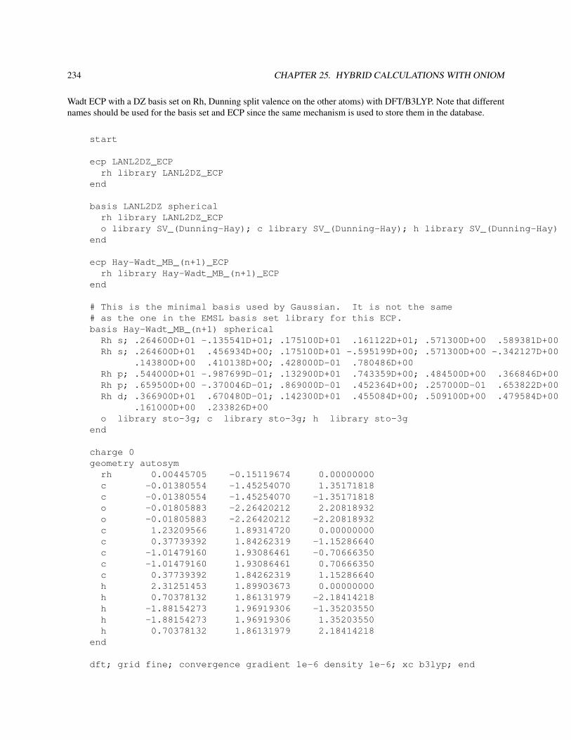
234 CHAPTER 25. HYBRID CALCULATIONS WITH ONIOM
Wadt ECP with a DZ basis set on Rh, Dunning split valence on the other atoms) with DFT/B3LYP. Note that differentnames should be used for the basis set and ECP since the same mechanism is used to store them in the database.
start
ecp LANL2DZ_ECPrh library LANL2DZ_ECP
end
basis LANL2DZ sphericalrh library LANL2DZ_ECPo library SV_(Dunning-Hay); c library SV_(Dunning-Hay); h library SV_(Dunning-Hay)
end
ecp Hay-Wadt_MB_(n+1)_ECPrh library Hay-Wadt_MB_(n+1)_ECP
end
# This is the minimal basis used by Gaussian. It is not the same# as the one in the EMSL basis set library for this ECP.basis Hay-Wadt_MB_(n+1) spherical
Rh s; .264600D+01 -.135541D+01; .175100D+01 .161122D+01; .571300D+00 .589381D+00Rh s; .264600D+01 .456934D+00; .175100D+01 -.595199D+00; .571300D+00 -.342127D+00
.143800D+00 .410138D+00; .428000D-01 .780486D+00Rh p; .544000D+01 -.987699D-01; .132900D+01 .743359D+00; .484500D+00 .366846D+00Rh p; .659500D+00 -.370046D-01; .869000D-01 .452364D+00; .257000D-01 .653822D+00Rh d; .366900D+01 .670480D-01; .142300D+01 .455084D+00; .509100D+00 .479584D+00
.161000D+00 .233826D+00o library sto-3g; c library sto-3g; h library sto-3g
end
charge 0geometry autosym
rh 0.00445705 -0.15119674 0.00000000c -0.01380554 -1.45254070 1.35171818c -0.01380554 -1.45254070 -1.35171818o -0.01805883 -2.26420212 2.20818932o -0.01805883 -2.26420212 -2.20818932c 1.23209566 1.89314720 0.00000000c 0.37739392 1.84262319 -1.15286640c -1.01479160 1.93086461 -0.70666350c -1.01479160 1.93086461 0.70666350c 0.37739392 1.84262319 1.15286640h 2.31251453 1.89903673 0.00000000h 0.70378132 1.86131979 -2.18414218h -1.88154273 1.96919306 -1.35203550h -1.88154273 1.96919306 1.35203550h 0.70378132 1.86131979 2.18414218
end
dft; grid fine; convergence gradient 1e-6 density 1e-6; xc b3lyp; end

25.6. EXAMPLES 235
scf; thresh 1e-6; end
oniomlow scf basis Hay-Wadt_MB_(n+1) ecp Hay-Wadt_MB_(n+1)_ECPhigh dft basis LANL2DZ ecp LANL2DZ_ECPmodel 5 charge 1print low
end
task oniom optimizetask oniom freq
25.6.3 A three-layer example
A three layer example combining CCSD(T), and MP2 with two different quality basis sets, and using multiple linkatoms.
The full system is tetra-dimethyl-amino-ethylene (TAME) or (N(Me)2)2-C=C-(N(Me)2)2. The intermediate sys-tem is (NH2)2-C=C-(NH2)2 and H2C=CH2 is the model system. CCSD(T)+aug-cc-pvtz is used for the model region,MP2+aug-cc-pvtz for the intermediate region, and MP2+aug-cc-pvdz for everything.
In the real geometry the first two atoms (C, C) are the model system (link atoms will be added automatically). Thefirst six atoms (C, C, N, N, N, N) describe the intermediate system (again with link atoms to be added automatically).The atoms have been numbered using comments to make the bonding input easier to generate.
To make the model system, four C-N bonds are broken between the ethylene fragment and the dimethyl-aminogroups and replaced with C-H bonds. To make the intermediate system, eight C-N bonds are broken between thenitrogens and the methyl groups and replaced with N-H bonds. The scaling factor could be chosen differently for eachof the bonds.
start
geometryC 0.40337795 -0.17516305 -0.51505208 # 1C -0.40328664 0.17555927 0.51466084 # 2N 1.87154979 -0.17516305 -0.51505208 # 3N -0.18694782 -0.60488524 -1.79258692 # 4N 0.18692927 0.60488318 1.79247594 # 5N -1.87148219 0.17564718 0.51496494 # 6C 2.46636552 1.18039452 -0.51505208 # 7C 2.48067731 -1.10425355 0.46161675 # 8C -2.46642715 -1.17982091 0.51473105 # 9C -2.48054940 1.10495864 -0.46156202 # 10C 0.30027136 0.14582197 -2.97072148 # 11C -0.14245927 -2.07576980 -1.96730852 # 12C -0.29948109 -0.14689874 2.97021079 # 13C 0.14140463 2.07558249 1.96815181 # 14H 0.78955302 2.52533887 1.19760764H -0.86543435 2.50958894 1.88075113... and 22 other hydrogen atoms on the methyl groups
end
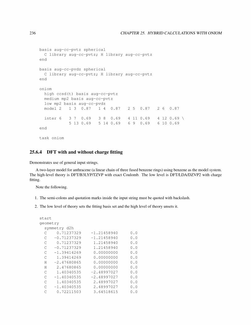
236 CHAPTER 25. HYBRID CALCULATIONS WITH ONIOM
basis aug-cc-pvtz sphericalC library aug-cc-pvtz; H library aug-cc-pvtz
end
basis aug-cc-pvdz sphericalC library aug-cc-pvtz; H library aug-cc-pvtz
end
oniomhigh ccsd(t) basis aug-cc-pvtzmedium mp2 basis aug-cc-pvtzlow mp2 basis aug-cc-pvdzmodel 2 1 3 0.87 1 4 0.87 2 5 0.87 2 6 0.87
inter 6 3 7 0.69 3 8 0.69 4 11 0.69 4 12 0.69 \5 13 0.69 5 14 0.69 6 9 0.69 6 10 0.69
end
task oniom
25.6.4 DFT with and without charge fitting
Demonstrates use of general input strings.
A two-layer model for anthracene (a linear chain of three fused benzene rings) using benzene as the model system.The high-level theory is DFT/B3LYP/TZVP with exact Coulomb. The low level is DFT/LDA/DZVP2 with chargefitting.
Note the following.
1. The semi-colons and quotation marks inside the input string must be quoted with backslash.
2. The low level of theory sets the fitting basis set and the high level of theory unsets it.
startgeometry
symmetry d2hC 0.71237329 -1.21458940 0.0C -0.71237329 -1.21458940 0.0C 0.71237329 1.21458940 0.0C -0.71237329 1.21458940 0.0C -1.39414269 0.00000000 0.0C 1.39414269 0.00000000 0.0H -2.47680865 0.00000000 0.0H 2.47680865 0.00000000 0.0C 1.40340535 -2.48997027 0.0C -1.40340535 -2.48997027 0.0C 1.40340535 2.48997027 0.0C -1.40340535 2.48997027 0.0C 0.72211503 3.64518615 0.0

25.6. EXAMPLES 237
C -0.72211503 3.64518615 0.0C 0.72211503 -3.64518615 0.0C -0.72211503 -3.64518615 0.0H 2.48612947 2.48094825 0.0H 1.24157357 4.59507342 0.0H -1.24157357 4.59507342 0.0H -2.48612947 2.48094825 0.0H 2.48612947 -2.48094825 0.0H 1.24157357 -4.59507342 0.0H -1.24157357 -4.59507342 0.0H -2.48612947 -2.48094825 0.0
end
basis smallh library DZVP_(DFT_Orbital)c library DZVP_(DFT_Orbital)
end
basis fittingh library DGauss_A1_DFT_Coulomb_Fittingc library DGauss_A1_DFT_Coulomb_Fitting
end
basis bigh library TZVP_(DFT_Orbital)c library TZVP_(DFT_Orbital)
end
oniommodel 8 1 9 0.75 2 10 0.75 3 11 0.75 4 12 0.75high dft basis big input "unset \"cd basis\"\; dft\; xc b3lyp\; end"low dft basis small input "set \"cd basis\" fitting\; dft\; xc\; end"
end
task oniom

238 CHAPTER 25. HYBRID CALCULATIONS WITH ONIOM

Chapter 26
Hessians
This section relates to the computation of analytic hessians which are available for open and closed shell SCF, exceptROHF and for closed shell DFT. Analytic hessians are not currently available for SCF or DFT calculations relativisticall-electron methodologies or for charge fitting with DFT. The current algorithm is fully in-core and does not usesymmetry. This will be changed in the next release.
There is no required input for the Hessian module. This module only impacts the hessian calculation. For optionsfor calculating the frequencies, please see Section 27, the Vibrational module.
26.1 Hessian Module Input
All input for the Hessian Module is optional since the default definitions are usually correct for most purposes. Thegeneric module input begins with hessian and has the form:
hessianthresh <real tol default 1d-6>print ...profile
end
26.1.1 Defining the wavefunction threshold
You may modify the default threshold for the wavefunction. This keyword is identical to THRESH in the SCF, Section10.7, and the CONVERGENCE gradient in the DFT, Section 11.7. The usual defaults for the convergence of thewavefunction for single point and gradient calculations is generally not tight enough for analytic hessians. Therefore,the hessian, by default, tightens these up to 1d-6 and runs an additional energy point if needed. If, during an analytichessian calculation, you encounter an error:
cphf_solve:the available MOs do not satisfy the SCF equations
the convergence criteria of the wavefunction generally needs to be tightened.
239

240 CHAPTER 26. HESSIANS
26.1.2 Profile
The PROFILE keyword provides additional information concerning the computation times of different sections of thehessian code. Summary information is given about the maximum, minimum and average times that a particular sectionof the code took to complete. This is normally only useful for developers.
26.1.3 Print Control
Known controllable print options are:
Name Print Level Description“hess_follow” high more information about where the calculation is“cphf_cont” debug detailed CPHF information“nucdd_cont” debug detailed nuclear contribution information“onedd_cont” debug detailed one electron contribution information“twodd_cont” debug detailed two electron contribution information“fock_xc” debug detailed XC information during the fock builds
Table 26.1: Hessian Print Control Specifications

Chapter 27
Vibrational frequencies
The nuclear hessian which is used to compute the vibrational frequencies can be computed by finite differencefor any ab initio wave-function that has analytic gradients or by analytic methods for SCF and DFT (see Sec-tion 26 for details). The appropriate nuclear hessian generation algorithm is chosen based on the user input whenTASK <theory> frequencies is the task directive.
The vibrational package was integrated from the Utah Messkit and can use any nuclear hessian generated fromthe driver routines, finite difference routines or any analytic hessian modules. There is no required input for the“VIB” package. VIB computes the Infra Red frequencies and intensities1 for the computed nuclear hessian and the“projected” nuclear hessian. The VIB module projects out the translations and rotations of the nuclear hessian usingthe standard Eckart projection algorithm. It also computes the zero point energy for the molecular system based onthe frequencies obtained from the projected hessian.
The default mass of each atom is used unless an alternative mass is provided via the geometry input, (c.f., 6)or redefined using the vibrational module input. The default mass is the mass of the most abundant isotope of eachelement.2 If the abundance was roughly equal, the mass of the isotope with the longest half life was used.
In addition, the vibrational analysis is given at the default standard temperature of 298.15 degrees.
27.1 Vibrational Module Input
All input for the Vibrational Module is optional since the default definitions will compute the frequencies and IRintensities3. The generic module input can begin with vib, freq, frequency and has the form:
{freq || vib || frequency}[reuse [<string hessian_filename>]][mass <integer lexical_index> <real new_mass>][mass <string tag_identifier> <real new_mass>][{temp || temperature} <integer number_of_temperatures> \
<real temperature1 temperature2 ...>][animate [<real step_size_for_animation>]]
1Intensities are only computed if the dipole derivatives are available; these are computed by default for most methods that use the finite differencedriver routines
2c.f., "The Elements" by John Emsley, Oxford University Press, (C) 1989, ISBN 0-19-855237-8.3The geometry specification at the point where the hessian is computed must be the default “geometry” on the current run-time-data-base for
the projection to work properly.
241

242 CHAPTER 27. VIBRATIONAL FREQUENCIES
end
27.1.1 Hessian File Reuse
By default the task <theory> frequencies directive will recompute the hessian. To reuse the previouslycomputed hessian you need only specify reuse in the module input block. If you have stored the hessian in analternate place you may redirect the reuse directive to that file by specifying the path to that file.
reuse /path_to_hessian_file
This will reuse your saved Hessian data but one caveat is that the geometry specification at the point where the hessianis computed must be the default “geometry” on the current run-time-data-base for the projection to work properly.
27.1.2 Redefining Masses of Elements
You may also modify the mass of a specific center or a group of centers via the input.
To modify the mass of a specific center you can simply use:
mass 3 4.00260324
which will set the mass of center 3 to 4.00260324 AMUs. The lexical index of centers is determined by the geometryobject.
To modify all Hydrogen atoms in a molecule you may use the tag based mechanism:
mass hydrogen 2.014101779
The mass redefinitions always start with the default masses and change the masses in the order given in the input.Care must be taken to change the masses properly. For example, if you want all hydrogens to have the mass ofDeuterium and the third hydrogen (which is the 6th atomic center) to have the mass of Tritium you must set theDeuterium masses first with the tag based mechanism and then set the 6th center’s mass to that of Tritium using thelexical center index mechanism.
The mass redefinitions are not fully persistent on the run-time-data-base. Each input block that redefines masseswill invalidate the mass definitions of the previous input block. For example,
freqreusemass hydrogen 2.014101779
endtask scf frequenciesfreq
reusemass oxygen 17.9991603
endtask scf frequencies
will use the new mass for all hydrogens in the first frequency analysis. The mass of the oxygen atoms will be redefinedin the second frequency analysis but the hydrogen atoms will use the default mass. To get a modified oxygen andhydrogen analysis you would have to use:

27.1. VIBRATIONAL MODULE INPUT 243
freqreusemass hydrogen 2.014101779
endtask scf frequenciesfreq
reusemass hydrogen 2.014101779mass oxygen 17.9991603
endtask scf frequencies
27.1.3 Temp or Temperature
The “VIB” module can generate the vibrational analysis at various temperatures other than at standard room tempera-ture. Either temp or temperature can be used to initiate this command.
To modify the temperature of the computation you can simply use:
temp 4 298.15 300.0 350.0 400.0
At this point, the temperatures are persistant and so the user must "reset" the temperature if the standard behavioris required after setting the temperatures in a previous “VIB” command, i.e.
temp 1 298.15
27.1.4 Animation
The “VIB” module also can generate mode animation input files in the standard xyz file format for graphics packageslike RasMol or XMol There are scripts to automate this for RasMol in $NWCHEM_TOP/contrib/rasmolmovie.Each mode will have 20 xyz files generated that cycle from the equilibrium geometry to 5 steps in the positive directionof the mode vector, back to 5 steps in the negative direction of the mode vector, and finally back to the equilibriumgeometry. By default these files are not generated. To activate this mechanism simply use the following input directive
animate
anywhere in the frequency/vib input block.
Controlling the Step Size Along the Mode Vector
By default, the step size used is 0.15 a.u. which will give reliable animations for most systems. This can be changedvia the input directive
animate real <step_size>
where <step_size> is the real number that is the magnitude of each step along the eigenvector of each nuclearhessian mode in atomic units.

244 CHAPTER 27. VIBRATIONAL FREQUENCIES
27.1.5 An Example Input Deck
This example input deck will optimize the geometry for the given basis set, compute the frequencies for H2O, H2O atdifferent temperatures, D2O, HDO, and TDO.
start h2otitle Watergeometry units au autosym
O 0.00000000 0.00000000 0.00000000H 0.00000000 1.93042809 -1.10715266H 0.00000000 -1.93042809 -1.10715266
endbasis noprint
H library sto-3gO library sto-3g
endscf; thresh 1e-6; enddriver; tight; endtask scf optimize
scf; thresh 1e-8; print none; endtask scf freq
freqreuse; temp 4 298.15 300.0 350.0 400.0
endtask scf freq
freqreuse; mass H 2.014101779temp 1 298.15
endtask scf freq
freqreuse; mass 2 2.014101779
endtask scf freq
freqreuse; mass 2 2.014101779 ; mass 3 3.01604927
endtask scf freq

Chapter 28
DPLOT
DPLOT...
END
This directive is used to obtain the plots of various types of electron densities (or orbitals) of the molecule. Theelectron density is calculated on a specified set of grid points using the molecular orbitals from SCF or DFT calculation.The output file is either in MSI Insight II contour format (default) or in the Gaussian Cube format. DPLOT is notexecuted until the “task dplot” directive is given. Different sub-directives are described below.
28.1 GAUSSIAN — Gaussian Cube format
GAUSSIAN
A outputfile is generate in Gaussian Cube format. You can visualize this file using gOpenMol (after converting theGaussian Cube file with gcube2plt), Molden or Molekel.
28.2 TITLE — Title directive
TITLE <string Title default Unknown Title>
This sub-directive specifies a title line for the generated input to the Insight program or for the Gaussian cube file.Only one line is allowed.
28.3 LIMITXYZ — Plot limits
LIMITXYZ [units <string Units default angstroms>]<real X_From> <real X_To> <integer No_Of_Spacings_X><real Y_From> <real Y_To> <integer No_Of_Spacings_Y><real Z_From> <real Z_To> <integer No_Of_Spacings_Z>
245

246 CHAPTER 28. DPLOT
This sub-directive specifies the limits of the cell to be plotted. The grid is generated using No_Of_Spacings + 1points along each direction. The known names for Units are angstroms, au and bohr.
28.4 SPIN — Density to be plotted
SPIN <string Spin default total>
This sub-directive specifies, what kind of density is to be computed. The known names for Spin are total,alpha, beta and spindens, the last being computed as the difference between α and β electron densities.
28.5 OUTPUT — Filename
OUTPUT <string File_Name default dplot>
This sub-directive specifies the name of the generated input to the Insight program or the generated Gaussian cubefile. The name OUTPUT is reserved for the standard NWChem output.
28.6 VECTORS — MO vector file name
VECTORS <string File_Name default movecs> [<string File_Name2>]
This sub-directive specifies the name of the molecular orbital file. If the second file is optionally given the densityis computed as the difference between the corresponding electron densities. The vector files have to match.
28.7 DENSMAT — Density matrix file name
DENSMAT <string File_Name> [<string File_Name2>]
This sub-directive specifies the name of density matrix file, and used for plotting the density generated by correla-tion methods, such as CCSD for ground state and EOM-CCSD for excited states.
The second file is optional. When it is given, the difference of the densities, specified by the two density matrixfiles, is computed and plotted.
28.8 WHERE — Density evaluation
WHERE <string Where default grid>
This sub-directive specifies where the density is to be computed. The known names for Where are grid (thecalculation of the density is performed on the set of a grid points specified by the sub-directive LimitXYZ and the filespecified by the sub-directive Output is generated), nuclei (the density is computed at the position of the nucleiand written to the NWChem output) and g+n (both).

28.9. ORBITAL — ORBITAL SUB-SPACE 247
28.9 ORBITAL — Orbital sub-space
ORBITALS [<string Option default density>]<integer No_Of_Orbitals><integer Orb_No_1 Orb_No_2 ...>
This sub-directive specifies the subset of the orbital space for the calculation of the electron density. The density iscomputed using the occupation numbers from the orbital file modified according to the Spin directive. If the contoursof the orbitals are to be plotted Option should be set to view. Note, that in this case No_Of_Orbitals should beset to 1 and sub-directive Where is automatically set to grid. Also specification of two orbital files conflicts withthe view option. α orbitals are always plotted unless Spin is set to beta.
28.10 Examples
Charge Density
Example of charge density plot (with Gaussian Cube output):
start n2geometry
n 0 0 0.53879155n 0 0 -0.53879155
endbasis; n library cc-pvdz;endscfvectors output n2.movecsenddplot
TITLE HOMOvectors n2.movecsLimitXYZ
-3.0 3.0 10-3.0 3.0 10-3.0 3.0 10
spin totalgaussianoutput lumo.cube
endtask scftask dplot
start n2geometry
n 0 0 0.53879155n 0 0 -0.53879155
endbasis; n library cc-pvdz;endscf

248 CHAPTER 28. DPLOT
vectors output n2.movecsend
tceccsddensmat n2.densmatend
task tce energy
dplotTITLE HOMOLimitXYZ
-3.0 3.0 10-3.0 3.0 10-3.0 3.0 10
spin totalgaussiandensmat n2.densmatoutput lumo.cube
endtask dplot
Molecular Orbital
Example of orbital plot (with Insight II contour output):
start n2geometry
n 0 0 0.53879155n 0 0 -0.53879155
endbasis; n library cc-pvdz;endscfvectors output n2.movecsenddplot
TITLE HOMOvectors n2.movecsLimitXYZ
-3.0 3.0 10-3.0 3.0 10-3.0 3.0 10
spin totalorbitals view; 1; 7output homo.grd
endtask scftask dplot

Chapter 29
Electron Transfer Calculations with ET
The NWChem electron transfer (ET) module calculates the electronic coupling energy (also called the electron transfermatrix element) between ET reactant and product states. The electronic coupling (VRP), activation energy (∆G∗), andnuclear reorganization energy (λ) are all components of the electron transfer rate defined by Marcus’ theory, whichalso depends on the temperature (reference 1):
kET =2π
hV 2
RP1√
4πλkBTexp(−∆G∗
kBT
)(29.1)
The ET module utilizes the method of Corresponding Orbital Transformation to calculate VRP. The only inputrequired are the names of the files containing the open-shell (UHF) MO vectors for the ET reactant and product states(R and P).
The basis set used in the calculation of VRP must be the same as the basis set used to calculate the MO vectors of Rand P. The magnitude of VRP depends on the amount of overlap between R and P, which is important to consider whenchoosing the basis set. Diffuse functions may be necessary to fill in the overlap, particularly when the ET distance islong.
The MO’s of R and P must correspond to localized states. for instance, in the reaction A− B→ A B− the transferringelectron is localized on A in the reactant state and is localized on B in the product state. To verify the localizationof the electron in the calculation of the vectors, carefully examine the Mulliken population analysis. In order todetermine which orbitals are involved in the electron transfer, use the print keyword "mulliken ao" which printsthe Mulliken population of each basis function.
An effective core potential (ECP) basis can be used to replace core electrons. However, there is one caveat: theorbitals involved in electron transfer must not be replaced with ECP’s. Since the ET orbitals are valence orbitals, thisis not usually a problem, but the user should use ECP’s with care.
Suggested references are listed below. The first two references gives a good description of Marcus’ two-state ETmodel, and the appendix of the third reference details the method used in the ET module.
1. R.A. Marcus, N. Sutin, Biochimica Biophysica Acta 35, 437, (1985).
2. J.R. Bolton, N. Mataga, and G. McLendon in “Electron Transfer in Inorganic, Organic and Biological Systems"(American Chemical Society, Washington, D.C., 1991)
3. A. Farazdel, M. Dupuis, E. Clementi, and A. Aviram, J. Am. Chem. Soc., 112, 4206 (1990).
249

250 CHAPTER 29. ELECTRON TRANSFER CALCULATIONS WITH ET
29.1 VECTORS — input of MO vectors for ET reactant and product states
VECTORS [reactants] <string reactants_filename>VECTORS [products ] <string products_filename>
In the VECTORS directive the user specifies the source of the molecular orbital vectors for the ET reactant andproduct states. This is required input, as no default filename will be set by the program. In fact, this is the only requiredinput in the ET module, although there are other optional keywords described below.
29.2 FOCK/NOFOCK — method for calculating the two-electron contribu-tion to VRP
<string (FOCK||NOFOCK) default FOCK>
This directive enables/disables the use of the NWChem’s Fock matrix routine in the calculation of the two-electronportion of the ET Hamiltonian. Since the Fock matrix routine has been optimized for speed, accuracy and parallelperformance, it is the most efficient choice.
Alternatively, the user can calculate the two-electron contribution to the ET Hamiltonian with another subroutinewhich may be more accurate for systems with a small number of basis functions, although it is slower.
29.3 TOL2E — integral screening threshold
TOL2E <real tol2e default max(10e-12,min(10e-7, S(RP)*10e-7 )>
The variable tol2e is used in determining the integral screening threshold for the evaluation of the two-electroncontribution to the Hamiltonian between the electron transfer reactant and product states. As a default, tol2e isset depending on the magnitude of the overlap between the ET reactant and product states (SRP), and is not less than1.0d-12 or greater than 1.0d-7.
The input to specify the threshold explicitly within the ET directive is, for example:
tol2e 1e-9
29.4 Example
The following example is for a simple electron transfer reaction, He → He+. The ET calculation is easy to execute,but it is crucial that ET reactant and product wavefunctions reflect localized states. This can be accomplished usingeither a fragment guess (shown in the example, see 10.5.1), or a charged atomic density guess (see 10.5.2). For self-exchange ET reactions such as this one, you can use the REORDER keyword to move the electron from the first heliumto the second (see 10.5).
Example input :

29.4. EXAMPLE 251
#ET reactants:charge 1scf
doublet; uhf; vectors input fragment HeP.mo He.mo output HeA.mo# HeP.mo are the vectors for He(+),# He.mo are the vectors for neutral He.endtask scf
#ET products:charge 1scf
doublet; uhf; vectors input HeA.mo reorder 2 1 output HeB.moendtask scf
etvectors reactants HeA.movectors products HeB.mo
endtask scf et
Here is what the output looks like for this example:
Electron Transfer Calculation-----------------------------
MO vectors for reactants: HeA.moMO vectors for products : HeB.mo
Electronic energy of reactants H(RR) -5.3402392824Electronic energy of products H(PP) -5.3402392824
Reactants/Products overlap S(RP) -0.0006033839
Reactants/Products interaction energy:-------------------------------------One-electron contribution H1(RP) 0.0040314092
Beginning calculation of 2e contributionTwo-electron integral screening (tol2e) : 6.03E-11
Two-electron contribution H2(RP) -0.0007837138Total interaction energy H(RP) 0.0032476955
Electron Transfer Coupling Energy |V(RP)| 0.00002548105.592 cm-1
0.000693 eV0.016 kcal/mol

252 CHAPTER 29. ELECTRON TRANSFER CALCULATIONS WITH ET
The overlap between the ET reactant and product states (SRP) is small, so the magnitude of the coupling betweenthe states is also small. If the fragment guess or charged atomic density guess were not used, the Mulliken spinpopulation would be 0.5 on both He atoms, the overlap between the ET reactant and product states would be 100 %and an infinite VRP would result.

Chapter 30
Properties
Properties can be calculated for both the Hartree-Fock and DFT wave functions. The properties that are available are:
• Natural bond analysis
• Dipole, quadrupole, and octupole moment
• Mulliken population analysis and bond order analysis
• Electrostatic potential (diamagnetic shielding) at nuclei
• Electric field and field gradient at nuclei
• Electron and spin density at nuclei
• NMR shielding (GIAO method)
• NMR hyperfine coupling (Fermi-Contact and Spin-Dipole expectation values)
• NMR indirect spin-spin coupling
The properties module is started when the task directive TASK <theory> property is defined in the userinput file. The input format has the form:
PROPERTY[property keyword][CENTER ((com || coc || origin || arb <real x y z>) default coc)]
END
Most of the properties can be computed for Hartree-Fock (closed-shell RHF, open-shell ROHF, and open-shellUHF), and DFT (closed-shell and open-shell spin unrestricted) wavefunctions. The NMR chemical shift is limitedto closed-shell wave functions, whereas the NMR hyperfine and indirect spin-spin coupling require a UHF or ODFTwave function.
253

254 CHAPTER 30. PROPERTIES
30.1 Property keywords
Each property can be requested by defining one of the following keywords:
NBOFILEDIPOLEQUADRUPOLEOCTUPOLEMULLIKENESPEFIELDEFIELDGRADELECTRONDENSITYHYPERFINESHIELDING [<integer> number_of_atoms <integer> atom_list]SPINSPIN [<integer> number_of_pairs <integer> pair_list]ALL
The “ALL” keyword generates all currently available properties.
Both the NMR shielding and spin-spin coupling have additional optional parameters that can be defined in theinput. For the shielding the user can define the number of atoms for which the shielding tensor should be calculated,followed by the list of specific atom centers. In the case of spin-spin coupling the number of atom pairs, followed bythe atom pairs, can be defined (i.e., spinspin 1 1 2 will calculate the coupling for one pair, and the coupling will bebetween atoms 1 and 2).
For both the NMR spin-spin and hyperfine coupling the isotope that has the highest abundance and has spin, willbe choosen for each atom under consideration.
The user also has the option to choose the center of expansion for the dipole, quadrupole, and octupole calculations.
[CENTER ((com || coc || origin || arb <real x y z>) default coc)]
com is the center of mass, coc is the center of charge, origin is (0.0, 0.0, 0.0) and arb is any arbitrary pointwhich must be accompanied by the coordinated to be used. Currently the x, y, and z coordinates must be given in thesame units as UNITS in GEOMETRY (See Section 6.1).
30.1.1 Nbofile
The keyword NBOFILE does not execute the Natural Bond Analysis code, but simply creates an input file to be usedas input to the stand-alone NBO code. All other properties are calculated upon request.
Following the successful completion of an electronic structure calculation, a Natural Bond Orbital (NBO) analysismay be carried out by providing the keyword NBOFILE in the PROPERTY directive. NWChem will query the rtdband construct an ASCII file, <file_prefix>.gen, that may be used as input to the stand alone version of the NBOprogram, gennbo. <file_prefix> is equal to string following the START directive. The input deck may be editedto provide additional options to the NBO calculation, (see the NBO user’s manual for details.)

Chapter 31
VSCF
The VSCF module can be used to calculate the anharmonic contributions to the vibrational modes of the molecule ofinterest. Energies are calculated on a one-dimensional grid along each normal mode, on a two-dimensional grid alongeach pair of normal modes, and optionally on a three-dimensional grid along each triplet of normal modes. Theseenergies are then used to calculate the vibrational nuclear wavefunction at an SCF- (VSCF) and MP2-like (cc-VSCF)level of theory.
VSCF can be used at all levels of theory, SCF and correlated methods, and DFT. For correlated methods, only theSCF level dipole is evaluated and used to calculate the IR intensity values.
The VSCF module is started when the task directive TASK <theory> vscf is defined in the user input file.The input format has the form:
VSCF[coupling <string couplelevel default "pair">][ngrid <integer default 16 >][iexcite <integer default 1 >][vcfct <real default 1.0>]
END
The order of coupling of the harmonic normal modes included in the calculation is controlled by the specifying:
coupling <string couplelevel default "pair">
For coupling=diagonal a one-dimensional grid along each normal mode is computed. For coupling=paira two-dimensional grid along each pair of normal modes is computed. For coupling=triplet a three-dimensionalgrid along each triplet of normal modes is computed.
The number of grid points along each normal mode, or pair of modes can be defined by specifying:
ngrid <integer default 16>
This VSCF module by default calculates the ground state (v=0), but can also calculate excited states (such as v=1).The number of excited states calculated is defined by specifying:
iexcite <integer default 1>
255

256 CHAPTER 31. VSCF
With iexcite=1 the fundamental frequencies are calculated. With iexcite=2 the first overtones are calcu-lated. With iexcite=3 the second overtones are calculated.
In certain cases the pair coupling potentials can become larger than those for a single normal mode. In this casethe pair potentials need to be scaled down. The scaling factor used can be defined by specifying:
vcfct <real default 1.0>

Chapter 32
Pseudopotential plane-wave densityfunctional theory (NWPW)
The NWChem plane-wave (NWPW) module uses pseudopotentials and plane-wave basis sets to perform DensityFunctional Theory calculations. This module complements the capabilities of the more traditional Gaussian functionbased approaches by having an accuracy at least as good for many applications, yet is still fast enough to treat systemscontaining hundreds of atoms. Another significant advantage is its ability to simulate dynamics on a ground statepotential surface directly at run-time using the Car-Parrinello algorithm. This method’s efficiency and accuracy makeit a desirable first principles method of simulation in the study of complex molecular, liquid, and solid state systems.Applications for this first principles method include the calculation of free energies, search for global minima, explicitsimulation of solvated molecules, and simulations of complex vibrational modes that cannot be described within theharmonic approximation.
The NWPW module is a collection of three modules.
• PSPW - (PSeudopotential Plane-Wave) A gamma point code for calculating molecules, liquids, crystals, andsurfaces.
• Band - A band structure code for calculating crystals and surfaces with small band gaps (e.g. semi-conductorsand metals).
• PAW - a (gamma point) projector augmented plane-wave code for calculating molecules, crystals, and surfaces
The PSPW, Band, and PAW modules can be used to compute the energy and optimize the geometry. Both the PSPWand Band modules can also be used to find saddle points, and compute numerical second derivatives. In addition thePSPW module can also be used to perform Car-Parrinello molecular dynamics.
Section 32.1 describes the tasks contained within the PSPW module, section 32.2 describes the tasks containedwithin the Band module, section 32.3 describes the tasks contained within the PAW module, and section 32.4 de-scribes the pseudopotential library included with NWChem. The datafiles used by the PSPW module are described insection 32.5. Car-Parrinello output data files are described in section 32.5.7, and the minimization and Car-Parrinelloalgorithms are described in section 32.6. Examples of how to setup and run a PSPW geometry optimization, a Car-Parrinello simulation, a band structure minimization, and a PAW geometry optimization are presented in sections32.7, 32.16, and 32.11, and 32.14. Finally in section 32.17 the capabilities and limitations of the NWPW module arediscussed.
If you are a first time user of this module it is recommended that you skip the next five sections and proceed directlyto the tutorials in sections 32.7-32.14.
257

258 CHAPTER 32. PSEUDOPOTENTIAL PLANE-WAVE DENSITY FUNCTIONAL THEORY (NWPW)
32.1 PSPW Tasks
All input to the PSPW Tasks is contained within the compound PSPW block,
PSPW...
END
To perform an actual calculation a TASK PSPW directive is used (Section 5.10).
TASK PSPW
In addition to the directives listed in Section 5.10, i.e.
TASK pspw energyTASK pspw gradientTASK pspw optimizeTASK pspw saddleTASK pspw freqenciesTASK pspw vib
there are additional directives that are specific to the PSPW module, which are:
TASK PSPW [Car-Parrinello ||pspw_dplot ||wannier ||psp_generator ||steepest_descent ||psp_formatter ||wavefunction_initializer ||v_wavefunction_initializer ||wavefunction_expander ]
Once a user has specified a geometry, the PSPW module can be invoked with no input directives (defaults invokedthroughout). However, the user will probably always specify the simulation cell used in the computation, since thedefault simulation cell is not well suited for most systems. There are sub-directives which allow for customizedapplication; those currently provided as options for the PSPW module are:
PSPWCELL_NAME <string cell_name default ’cell_default’>INPUT_WAVEFUNCTION_FILENAME <string input_wavefunctions default input_movecs>OUTPUT_WAVEFUNCTION_FILENAME <string output_wavefunctions default input_movecs>FAKE_MASS <real fake_mass default 400000.0>TIME_STEP <real time_step default 5.8>LOOP <integer inner_iteration outer_iteration default 10 100>TOLERANCES <real tole tolc default 1.0e-7 1.0e-7>CUTOFF <real cutoff>ENERGY_CUTOFF <real ecut default (see input description)>WAVEFUNCTION_CUTOFF <real wcut default (see input description)>EWALD_NCUT <integer ncut default 1>]

32.1. PSPW TASKS 259
EWALD_RCUT <real rcut default (see input description)>XC (Vosko || LDA || PBE96 || revPBE || HF || PBE0 || revPBE0 ||
LDA-SIC || LDA-SIC/2 || LDA-0.4SIC || LDA-SIC/4 || LDA-0.2SIC ||PBE96-SIC || PBE96-SIC/2 || PBE96-0.4SIC || PBE96-SIC/4 || PBE96-0.2SIC ||revPBE-SIC || revPBE-SIC/2 || revPBE-0.4SIC || revPBE-SIC/4 || revPBE-0.2SIC ||default Vosko)
DFT||ODFT||RESTRICTED||UNRESTRICTEDMULT <integer mult default 1>MULLIKENEFIELDALLOW_TRANSLATIONCGLMBFGSSCF [Anderson|| simple || Broyden]
[CG || RMM-DIIS][density || potential][ALPHA real alpha default 0.25][ITERATIONS integer inner_iterations default 5][OUTER_ITERATIONS integer outer_iterations default 0]
SIMULATION_CELL ... (see input description) ENDDPLOT ... (see input description) ENDWANNIER ... (see input description) ENDCAR-PARRINELLO ... (see input description) ENDPSP_GENERATOR ... (see input description) ENDWAVEFUNCTION_INITIALIZER ... (see input description) ENDV_WAVEFUNCTION_INITIATIZER ... (see input description) ENDWAVEFUNCTION_EXPANDER ... (see input description) ENDSTEEPEST_DESCENT ... (see input description) END
MAPPING <integer mapping default 1>
ROTATION (ON || OFF)TRANSLATION (ON || OFF)
END
The following list describes the keywords contained in the PSPW input block.
• <cell_name> - name of the simulation_cell named <cell_name>. See section 32.1.1.
• <input_wavefunctions> - name of the file containing one-electron orbitals
• <output_wavefunctions> - name of the file that will contain the one-electron orbitals at the end of the run.
• <fake_mass> - value for the electronic fake mass (µ). This parameter is not presently used in a conjugategradient simulation
• <time_step> - value for the time step (∆t). This parameter is not presently used in a conjugate gradient simu-lation.
• <inner_iteration> - number of iterations between the printing out of energies and tolerances

260 CHAPTER 32. PSEUDOPOTENTIAL PLANE-WAVE DENSITY FUNCTIONAL THEORY (NWPW)
• <outer_iteration> - number of outer iterations
• <tole> - value for the energy tolerance.
• <tolc> - value for the one-electron orbital tolerance.
• <cutoff> - value for the cutoff energy used to define the wavefunction. In addition using the CUTOFF keywordautomatically sets the cutoff energy for the density to be twice the wavefunction cutoff.
• <ecut> - value for the cutoff energy used to define the density. Default is set to be the maximum value that willfit within the simulation_cell <cell_name>.
• <wcut> - value for the cutoff energy used to define the one-electron orbitals. Default is set to be the maximumvalue that will fit within the simulation_cell <cell_name>.
• <ncut> - value for the number of unit cells to sum over (in each direction) for the real space part of the Ewaldsummation. Note Ewald summation is only used if the simulation_cell is periodic.
• <rcut> - value for the cutoff radius used in the Ewald summation. Note Ewald summation is only used if thesimulation_cell is periodic.Default set to be MIN(|~ai|)
π, i = 1,2,3.
• (Vosko || PBE96 || revPBE || ...) - Choose between Vosko et al’s LDA parameterization or the orginal andrevised Perdew, Burke, and Ernzerhof GGA functional. In addition, several hybrid options.
• MULT - optional keyword which if specified allows the user to define the spin multiplicity of the system
• MULLIKEN - optional keyword which if specified causes a Mulliken analysis to be performed at the end of thesimulation.
• ALLOW_TRANSLATION - By default the the center of mass forces are projected out of the computed forces.This optional keyword if specified allows the center of mass forces to not be zero.
• CG - optional keyword which sets the minimizer to 1
• LMBFGS - optional keyword which sets the minimizer to 2
• SCF - optional keyword which sets the minimizer to be a band by band minimizer. Several options are availablefor setting the density or potential mixing, and the type of Kohn-Sham minimizer.
• SIMULATION_CELL (see section 32.1.1)
• DPLOT (see section 32.2.2)
• WANNIER (see section 32.1.4)
• CAR-PARRINELLO(see section 32.1.7)
• PSP_GENERATOR (see section 32.1.10)
• WAVEFUNCTION_INITIALIZER (see section 32.1.11)
• V_WAVEFUNCTION_INITIALIZER (see section 32.1.12)
• WAVEFUNCTION_EXPANDER (see section 32.1.13).
• STEEPEST_DESCENT (see section 32.1.14)
• <mapping> - for a value of 1 slab FFT is used, for a value of 2 a 2d-hilbert FFT is used.

32.1. PSPW TASKS 261
A prototype limited memory BFGS (LMBFGS) minimizer can be used to minimize the energy. To use this newoptimizer the following SET directive needs to be specified:
set nwpw:mimimizer 1 # Default - Grassman conjugate gradient minimizer is used to minimize the energy.set nwpw:mimimizer 2 # Grassman LMBFGS minimimzer is used to minimize the energy.set nwpw:minimizer 4 # Stiefel conjugate gradient minimizer is used to minimize the energy.set nwpw:minimizer 5 # Band-by-band minimizer is used to minimize the energy.
Limited testing suggests that the Grassman LMBFGS minimizer is about twice as fast as the conjugate gradientminimizer. However, there are several known cases where this optimizer fails, so it is currently not a default option,and should be used with caution.
In addition the following SET directives can be specified:
set nwpw:lcao_skip .false. # Default - initial wavefunctions generated using an LCAO guess.set nwpw:lcao_skip .true. # Initial wavefunctions generated using a random plane-wave guess.
set nwpw:lcao_print .false. # Default - Ouput not produced during the generation of the LCAO guess.set nwpw:lcao_print .true. # Output produced during the generation of the LCAO guess.
set nwpw:lcao_iterations 2 #specifies the number of LCAO iterations
32.1.1 Simulation Cell
The simulation cell parameters are entered by defining a simulation_cell sub-block within the PSPW block. Listedbelow is the format of a simulation_cell sub-block.
PSPW...
SIMULATION_CELLCELL_NAME <string name default ’cell_default’>BOUNDARY_CONDITIONS (periodic || aperiodic default periodic)LATTICE_VECTORS
<real a1.x a1.y a1.z default 20.0 0.0 0.0><real a2.x a2.y a2.z default 0.0 20.0 0.0><real a3.x a3.y a3.z default 0.0 0.0 20.0>
NGRID <integer na1 na2 na3 default 32 32 32>END
...END
Basically, the user needs to enter the dimensions, gridding and boundary conditions of the simulation cell. Thefollowing list describes the input in detail.
• <name> - user-supplied name for the simulation block.
• periodic - keyword specifying that the simulation cell has periodic boundary conditions.
• aperiodic - keyword specifying that the simulation cell has free-space boundary conditions.
• <a1.x a1.y a1.z> - user-supplied values for the first lattice vector

262 CHAPTER 32. PSEUDOPOTENTIAL PLANE-WAVE DENSITY FUNCTIONAL THEORY (NWPW)
• <a2.x a2.y a2.z> - user-supplied values for the second lattice vector
• <a3.x a3.y a3.z> - user-supplied values for the third lattice vector
• <na1 na2 na3> - user-supplied values for discretization along lattice vector directions.
Alternatively, instead of explicitly entering lattice vectors, users can enter the unit cell using the standard cellparameters, a, b, c, α, β, and γ, by using the LATTICE block. The format for input is as follows:
PSPW...
SIMULATION_CELL...LATTICE
[lat_a <real a default 20.0>][lat_b <real b default 20.0>][lat_c <real c default 20.0>][alpha <real alpha default 90.0>][beta <real beta default 90.0>][gamma <real gamma default 90.0>]
END...
END...END
The user can also enter the lattice vectors of standard unit cells using the keywords SC, FCC, BCC, for simplecubic, face-centered cubic, and body-centered cubic respectively. Listed below is an example of the format of this typeof input.
PSPW...
SIMULATION_CELLSC 20.0....
END...END
Finally, the lattice vectors from the unit cell can also be defined using the fractional coordinate input in the GE-OMETRY input (see section 6.7). Listed below is an example of the format of this type of input for an 8 atom siliconcarbide unit cell.
geometry units ausystem crystal
lat_a 8.277d0lat_b 8.277d0lat_c 8.277d0alpha 90.0d0beta 90.0d0gamma 90.0d0

32.1. PSPW TASKS 263
endSi -0.50000d0 -0.50000d0 -0.50000d0Si 0.00000d0 0.00000d0 -0.50000d0Si 0.00000d0 -0.50000d0 0.00000d0Si -0.50000d0 0.00000d0 0.00000d0C -0.25000d0 -0.25000d0 -0.25000d0C 0.25000d0 0.25000d0 -0.25000d0C 0.25000d0 -0.25000d0 0.25000d0C -0.25000d0 0.25000d0 0.25000d0end
32.1.2 Unit Cell Optimization
The PSPW module using the DRIVER geometry optimizer can optimize a crystal unit cell. Currently this type ofoptimization works only if the geometry is specified in fractional coordinates. The following SET directive is used totell the DRIVER geometry optimizer to optimize the crystal unit cell in addition to the geometry.
set includestress .true.
32.1.3 DPLOT
The pspw dplot task is used to generate plots of various types of electron densities (or orbitals) of a molecule. Theelectron density is calculated on the specified set of grid points from a PSPW calculation. The output file generated isin the Gaussian Cube format. Input to the DPLOT task is contained within the DPLOT sub-block.
PSPW...DPLOT
...END...
END
To run a DPLOT calculation the following directive is used:
TASK PSPW PSPW_DPLOT
Listed below is the format of a DPLOT sub-block.
PSPW...
DPLOTVECTORS <string input_wavefunctions default input_movecs>DENSITY [total||difference||alpha||beta||laplacian||potential default total] <string density_name no default>ELF [restricted|alpha|beta] <string elf_name no default>ORBITAL <integer orbital_number no default> <string orbital_name no default>
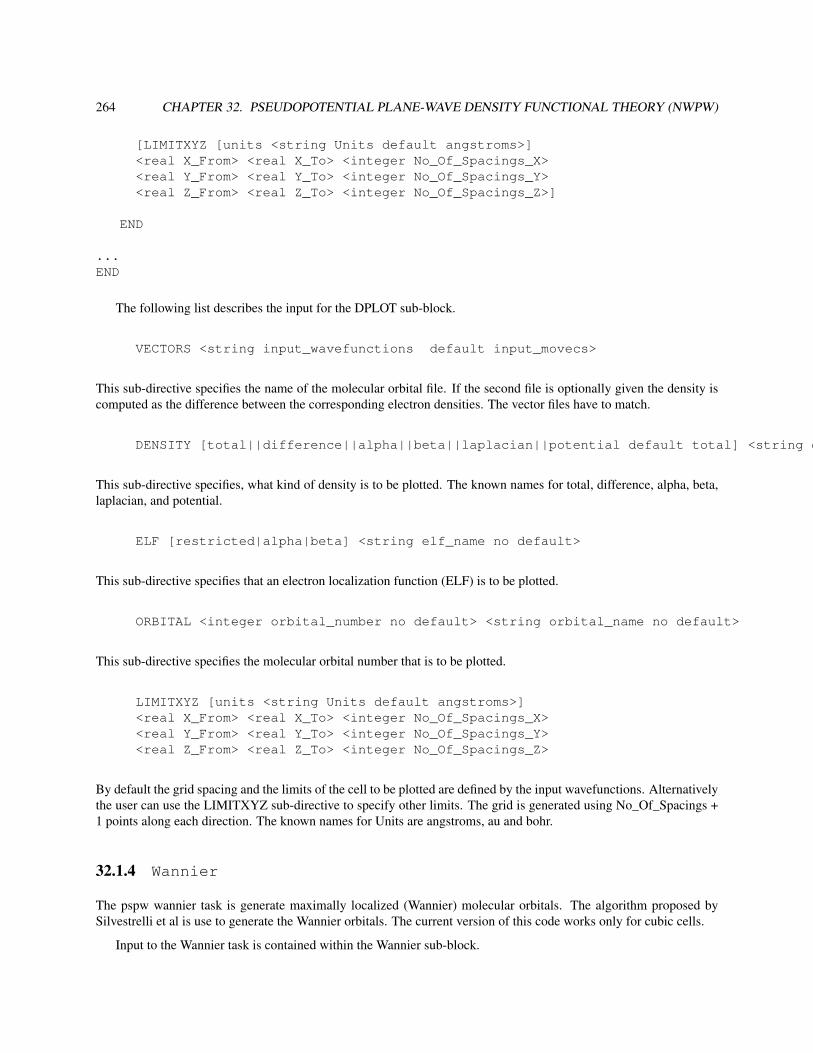
264 CHAPTER 32. PSEUDOPOTENTIAL PLANE-WAVE DENSITY FUNCTIONAL THEORY (NWPW)
[LIMITXYZ [units <string Units default angstroms>]<real X_From> <real X_To> <integer No_Of_Spacings_X><real Y_From> <real Y_To> <integer No_Of_Spacings_Y><real Z_From> <real Z_To> <integer No_Of_Spacings_Z>]
END
...END
The following list describes the input for the DPLOT sub-block.
VECTORS <string input_wavefunctions default input_movecs>
This sub-directive specifies the name of the molecular orbital file. If the second file is optionally given the density iscomputed as the difference between the corresponding electron densities. The vector files have to match.
DENSITY [total||difference||alpha||beta||laplacian||potential default total] <string density_name no default>
This sub-directive specifies, what kind of density is to be plotted. The known names for total, difference, alpha, beta,laplacian, and potential.
ELF [restricted|alpha|beta] <string elf_name no default>
This sub-directive specifies that an electron localization function (ELF) is to be plotted.
ORBITAL <integer orbital_number no default> <string orbital_name no default>
This sub-directive specifies the molecular orbital number that is to be plotted.
LIMITXYZ [units <string Units default angstroms>]<real X_From> <real X_To> <integer No_Of_Spacings_X><real Y_From> <real Y_To> <integer No_Of_Spacings_Y><real Z_From> <real Z_To> <integer No_Of_Spacings_Z>
By default the grid spacing and the limits of the cell to be plotted are defined by the input wavefunctions. Alternativelythe user can use the LIMITXYZ sub-directive to specify other limits. The grid is generated using No_Of_Spacings +1 points along each direction. The known names for Units are angstroms, au and bohr.
32.1.4 Wannier
The pspw wannier task is generate maximally localized (Wannier) molecular orbitals. The algorithm proposed bySilvestrelli et al is use to generate the Wannier orbitals. The current version of this code works only for cubic cells.
Input to the Wannier task is contained within the Wannier sub-block.

32.1. PSPW TASKS 265
PSPW...Wannier
...END...
END
To run a Wannier calculation the following directive is used:
TASK PSPW Wannier
Listed below is the format of a Wannier sub-block.
PSPW...
WannierOLD_WAVEFUNCTION_FILENAME <string input_wavefunctions default input_movecs>NEW_WAVEFUNCTION_FILENAME <string output_wavefunctions default input_movecs>
END...END
The following list describes the input for the Wannier sub-block.
• <input_wavefunctions> - name of pspw wavefunction file.
• <output_wavefunctions> - name of pspw wavefunction file that will contain the Wannier orbitals.
32.1.5 Self-Interaction Corrections
The SET directive is used to specify the molecular orbitals contribute to the self-interaction-correction (SIC) term.
set pspw:SIC_orbitals <integer list_of_molecular_orbital_numbers>
This defines only the molecular orbitals in the list as SIC active. All other molecular orbitals will not contribute to theSIC term.
For example the following directive specifies that the molecular orbitals numbered 1,5,6,7,8, and 15 are SIC active.
set pspw:SIC_orbitals 1 5:8 15
or equivalently
set pspw:SIC_orbitals 1 5 6 7 8 15
The following directive turns on self-consistent SIC.
set pspw:SIC_relax .false. # Default - Perturbative SIC calculationset pspw:SIC_relax .true. # Self-consistent SIC calculation

266 CHAPTER 32. PSEUDOPOTENTIAL PLANE-WAVE DENSITY FUNCTIONAL THEORY (NWPW)
Two types of solvers can be used and they are specified using the following SET directive
set pspw:SIC_solver_type 1 # Default - cutoff coulomb kernelset pspw:SIC_solver_type 2 # Free-space boundary condition kernel
The parameters for the cutoff coulomb kernel are defined by the following SET directives:
set pspw:SIC_screening_radius <real rcut>set pspw:SIC_screening_power <real rpower>
32.1.6 Point Charge Analysis
The MULLIKEN option can be used to generate derived atomic point charges from a plane-wave density. Thisanalysis is based on a strategy suggested in the work of P.E. Blochl, J. Chem. Phys. vol. 103, page 7422 (1995).In this strategy the low-frequency components a plane-wave density are fit to a linear combination of atom centeredGaussian functions.
The following SET directives are used to define the fitting.
set pspw_APC:Gc <real Gc_cutoff> # specifies the maximum frequency component of the density to be used in the fitting in units of au.
set pspw_APC:nga <integer number_gauss> # specifies the the number of Gaussian functions peratom.
set pspw_APC:gamma <real gamma_list> # specifies the decay lengths of each atom centered Gaussian.
We suggest using the following parameters.
set pspw_APC:Gc 2.5set pspw_APC:nga 3set pspw_APC:gamma 0.6 0.9 1.35
32.1.7 Car-Parrinello
The Car-Parrinello task is used to perform ab initio molecular dynamics using the scheme developed by Car andParrinello. In this unified ab initio molecular dynamics scheme the motion of the ion cores is coupled to a fictitiousmotion for the Kohn-Sham orbitals of density functional theory. Constant energy or constant temperature simulationscan be performed. A detailed description of this method is described in section 32.6.
Input to the Car-Parrinello simulation is contained within the Car-Parrinello sub-block.
PSPW...Car-Parrinello
...END...
END
To run a Car-Parrinello calculation the following directive is used:

32.1. PSPW TASKS 267
TASK PSPW Car-Parrinello
The Car-Parrinello sub-block contains a great deal of input, including pointers to data, as well as parameter input.Listed below is the format of a Car-Parrinello sub-block.
PSPW...
Car-ParrinelloCELL_NAME <string cell_name default ’cell_default’>INPUT_WAVEFUNCTION_FILENAME <string input_wavefunctions default input_movecs>OUTPUT_WAVEFUNCTION_FILENAME <string output_wavefunctions default input_movecs>INPUT_V_WAVEFUNCTION_FILENAME <string input_v_wavefunctions default input_vmovecs>OUTPUT_V_WAVEFUNCTION_FILENAME <string output_v_wavefunctions default input_vmovecs>FAKE_MASS <real fake_mass default default 1000.0>TIME_STEP <real time_step default 5.0>LOOP <integer inner_iteration outer_iteration default 10 1>SCALING <real scale_c scale_r default 1.0 1.0>ENERGY_CUTOFF <real ecut default (see input description)>WAVEFUNCTION_CUTOFF <real wcut default (see input description)>EWALD_NCUT <integer ncut default 1>EWALD_RCUT <real rcut default (see input description)>XC (Vosko || LDA || PBE96 || revPBE || HF || PBE0 || revPBE0 ||
LDA-SIC || LDA-SIC/2 || LDA-0.4SIC || LDA-SIC/4 || LDA-0.2SIC ||PBE96-SIC || PBE96-SIC/2 || PBE96-0.4SIC || PBE96-SIC/4 || PBE96-0.2SIC ||revPBE-SIC || revPBE-SIC/2 || revPBE-0.4SIC || revPBE-SIC/4 || revPBE-0.2SIC ||default Vosko)
[Nose-Hoover <real Period_electron Temperature_electrion Period_ion Temperature_iondefault 100.0 298.15 100.0 298.15>]
[SA_decay <real sa_scale_c sa_scale_r default 1.0 1.0>]XYZ_FILENAME <string xyz_filename default XYZ>EMOTION_FILENAME <string emotion_filename default EMOTION>HMOTION_FILENAME <string hmotion_filename default HMOTION>OMOTION_FILENAME <string omotion_filename default OMOTION>EIGMOTION_FILENAME <string eigmotion_filename default EIGMOTION>ION_MOTION_FILENAME <string ion_motion_filename default MOTION>
END...
END
The following list describes the input for the Car-Parrinello sub-block.
• <cell_name> - name of the the simulation_cell named <cell_name>. See section 32.1.1.
• <input_wavefunctions> - name of the file containing one-electron orbitals
• <output_wavefunctions> - name of the file that will contain the one-electron orbitals at the end of the run.
• <input_v_wavefunctions> - name of the file containing one-electron orbital velocities.
• <output_v_wavefunctions> - name of the file that will contain the one-electron orbital velocities at the end ofthe run.

268 CHAPTER 32. PSEUDOPOTENTIAL PLANE-WAVE DENSITY FUNCTIONAL THEORY (NWPW)
• <fake_mass> - value for the electronic fake mass (µ).
• <time_step> - value for the Verlet integration time step (∆t).
• <inner_iteration> - number of iterations between the printing out of energies.
• <outer_iteration> - number of outer iterations
• <scale_c> - value for the initial velocity scaling of the one-electron orbital velocities.
• <scale_r> - value for the initial velocity scaling of the ion velocities.
• <ecut> - value for the cutoff energy used to define the density. Default is set to be the maximum value that willfit within the simulation_cell <cell_name>.
• <wcut> - value for the cutoff energy used to define the one-electron orbitals. Default is set to be the maximumvalue that will fit within the simulation_cell <cell_name>.
• <ncut> - value for the number of unit cells to sum over (in each direction) for the real space part of the Ewaldsummation. Note Ewald summation is only used if the simulation_cell is periodic.
• <rcut> - value for the cutoff radius used in the Ewald summation. Note Ewald summation is only used if thesimulation_cell is periodic.Default set to be MIN(|~ai|)
π, i = 1,2,3.
• (Vosko || PBE96 || revPBE || ...) - Choose between Vosko et al’s LDA parameterization or the orginal andrevised Perdew, Burke, and Ernzerhof GGA functional. In addition, several hybrid options.
• Nose-Hoover - optional subblock which if specified causes the simulation to perform Nose-Hoover dynamics.If this subblock is not specified the simulation performs constant energy dynamics. See section 32.6.2 for adescription of the parameters.
– <Period_electron> ≡ Pelectron - estimated period for fictitious electron thermostat.
– <Temperature_electron> ≡ Telectron - temperature for fictitious electron motion
– <Period_ion> ≡ Pion - estimated period for ionic thermostat
– <Temperature_ion> ≡ Tion - temperature for ion motion
• SA_decay - optional subblock which if specified causes the simulation to run a simulated annealing simulation.For simulated annealing to work the Nose-Hoover subblock needs to be specified. The initial temperature aretaken from the Nose-Hoover subblock. See section 32.6.2 for a description of the parameters.
– <sa_scale_c> ≡ τelectron - decay rate in atomic units for electronic temperature.
– <sa_scale_r> ≡ τionic - decay rate in atomic units for the ionic temperature.
• <xyz_filename> - name of the XYZ motion file generated
• <emotion_filename> - name of the emotion motion file. See section 32.5.7 for a description of the datafile.
• <hmotion_filename> - name of the hmotion motion file. See section 32.5.7 for a description of the datafile.
• <eigmotion_filename> - name of the eigmotion motion file. See section 32.5.7 for a description of the datafile.
• <ion_motion_filename> - name of the ion_motion motion file. See section 32.5.7 for a description of thedatafile.
• MULLIKEN - optional keyword which if specified causes an omotion motion file to be created.

32.1. PSPW TASKS 269
• <omotion_filename> - name of the omotion motion file. See section 32.5.7 for a description of the datafile.
When a DPLOT sub-block is specified the following SET directive can be used to output dplot data during aCar-Parrinello simulation:
set pspw_dplot:iteration_list <integer list_of_iteration_numbers>
The Gaussian cube files specified in the DPLOT sub-block are appended with the specified iteration number.
For example, the following directive specifies that at the 3,10,11,12,13,14,15, and 50 iterations Gaussian cube filesare to be produced.
set pspw_dplot:iteration_list 3,10:15,50
32.1.8 Adding Geometry Constraints To A Car-Parrinello Simulation
The Car-Parrinello module allows users to freeze the cartesian coordinates in a simulation (Note - the Car-Parrinellocode recognizes Cartesian constraints, but it does not recognize internal coordinate constraints). The SET directive(Section 6.6) is used to freeze atoms, by specifying a directive of the form:
set geometry:actlist <integer list_of_center_numbers>
This defines only the centers in the list as active. All other centers will have zero force assigned to them, and willremain frozen at their starting coordinates during a Car-Parrinello simulation.
For example, the following directive specifies that atoms numbered 1, 5, 6, 7, 8, and 15 are active and all otheratoms are frozen:
set geometry:actlist 1 5:8 15
or equivalently,
set geometry:actlist 1 5 6 7 8 15
If this option is not specified by entering a SET directive, the default behavior in the code is to treat all atoms asactive. To revert to this default behavior after the option to define frozen atoms has been invoked, the UNSET directivemust be used (since the database is persistent, see Section 3.2). The form of the UNSET directive is as follows:
unset geometry:actlist
In addition, the Car-Parrinello module allows users to freeze bond lengths via a Shake algorithm. The followingSET directive shows how to do this.
set nwpw:shake_constraint "2 6 L 6.9334"
This input fixes the bond length between atoms 2 and 6 to be 6.9334 bohrs. Note that this input only recognizes bohrs.
When using constraints it is usually necessary to turn off center of mass shifting. This can be done by the followingSET directive.
set nwpw:com_shift .false.

270 CHAPTER 32. PSEUDOPOTENTIAL PLANE-WAVE DENSITY FUNCTIONAL THEORY (NWPW)
32.1.9 QM/MM
A preliminary QM/MM capability that can run Car-Parrinello molecular dynamics has been integrated into the PSPWmodule. Currently, the input is not very robust but it is straightforward. The first step to run a QM/MM simulations isto define the MM atoms in the geometry block. The MM atoms must be at the end of the geometry and a carat, " ˆ ",must be appended to the end of the atom name, e.g.
geometry units angstrom nocenter noautosym noautoz print xyzC -0.000283 0.000106 0.000047Cl -0.868403 1.549888 0.254229Cl 0.834043 -0.474413 1.517103Cl -1.175480 -1.275747 -0.460606Cl 1.209940 0.200235 -1.310743
O^ 0.3226E+01 -0.4419E+01 -0.5952E+01H^ 0.3193E+01 -0.4836E+01 -0.5043E+01H^ 0.4167E+01 -0.4428E+01 -0.6289E+01O^ 0.5318E+01 -0.3334E+01 -0.1220E+01H^ 0.4978E+01 -0.3040E+01 -0.2113E+01H^ 0.5654E+01 -0.2540E+01 -0.7127E+00end
Next the pseudopotentials have be defined for the every type of MM atom contained in the geometry blocks. Thefollowing local pseudopotential suggested by Laio, VandeVondele and Rothlisberger can be automatically generated.
V (~r) =−Zionrc
nσ − rnσ
−sign(Zion)∗ rcnσ+1− rnσ+1 (32.1)
The following input To define this pseudopo the Oˆ MM atom using the following input
NWPWQMMM
mm_psp O^ -0.8476 4 0.70END
END
defines the local pseudopotential for the Oˆ MM atom , where Zion = −0.8476, nσ = 4, and rc = 0.7. The followinginput can be used to define the local pseudopotentials for all the MM atoms in the geometry block defined above
NWPWQMMM
mm_psp O^ -0.8476 4 0.70mm_psp H^ 0.4238 4 0.40
ENDEND
Next the Lenard-Jones potentials for the QM and MM atoms need to be defined. This is done as as follows
NWPWQMMM

32.1. PSPW TASKS 271
lj_ion_parameters C 3.41000000d0 0.10d0lj_ion_parameters Cl 3.45000000d0 0.16d0lj_ion_parameters O^ 3.16555789d0 0.15539425d0
ENDEND
Note that the Lenard-Jones potential is not defined for the MM H atoms in this example. The final step is to definethe MM fragments in the simulation. MM fragments are a set of atoms in which bonds and angle harmonic potentialsare defined, or alternatively shake constraints are defined. The following input defines the fragments for the two watermolecules in the above geometry,
NWPWQMMM
fragment spcsize 3 #size of fragmentindex_start 6:9:3 #atom index list that defines the start of
# the fragments (start:final:stride)
bond_spring 1 2 0.467307856 1.889726878 #bond i j Kspring r0bond_spring 1 3 0.467307856 1.889726878 #bond i j Kspring r0angle_spring 2 1 3 0.07293966 1.910611932 #angle i j k Kspring theta0
endEND
END
The fragments can be defined using shake constraints as
NWPWQMMM
fragment spcsize 3 #size of fragmentindex_start 6:9:3 #atom index list that defines the start of
# the fragments (start:final:stride)
shake units angstroms 1 2 3 cyclic 1.0 1.632993125 1.0end
ENDEND
Alternatively, each water could be defined independently as follows.
NWPWQMMM
fragment spc1size 3 #size of fragmentindex_start 6 #atom index list that defines the start of
#the fragments
bond_spring 1 2 0.467307856 1.889726878 #bond i j Kspring r0bond_spring 1 3 0.467307856 1.889726878 #bond i j Kspring r0angle_spring 2 1 3 0.07293966 1.910611932 #angle i j k Kspring theta0

272 CHAPTER 32. PSEUDOPOTENTIAL PLANE-WAVE DENSITY FUNCTIONAL THEORY (NWPW)
endfragment spc2
size 3 #size of fragmentindex_start 9 #atom index list that defines the start of
#the fragmentsshake units angstroms 1 2 3 cyclic 1.0 1.632993125 1.0
endEND
END
32.1.10 PSP_GENERATOR
A one-dimensional pseudopotential code has been integrated into NWChem. This code allows the user to modify anddevelop pseudopotentials. Currently, only the Hamann and Troullier-Martins norm-conserving pseudopotentials canbe generated. In future releases, the pseudopotential library (section 32.4) will be more complete, so that the user willnot have explicitly generate pseudopotentials using this module.
Input to the PSP_GENERATOR task is contained within the PSP_GENERATOR sub-block.
PSPW...PSP_GENERATOR
...END...
END
To run a PSP_GENERATOR calculation the following directive is used:
TASK PSPW PSP_GENERATOR
Listed below is the format of a PSP_GENERATOR sub-block.
PSPW...
PSP_GENERATORPSEUDOPOTENTIAL_FILENAME: <string psp_name>ELEMENT: <string element>CHARGE: <real charge>MASS_NUMBER: <real mass_number>ATOMIC_FILLING: <integer ncore nvalence>( (1||2||...) (s||p||d||f||...) <real filling> \
...)
[CUTOFF: <integer lmax>( (s||p||d||f||g) <real rcut>\...)
]PSEUDOPOTENTIAL_TYPE: (TROULLIER-MARTINS || HAMANN default HAMANN)SOLVER_TYPE: (PAULI || SCRHODINGER default PAULI)
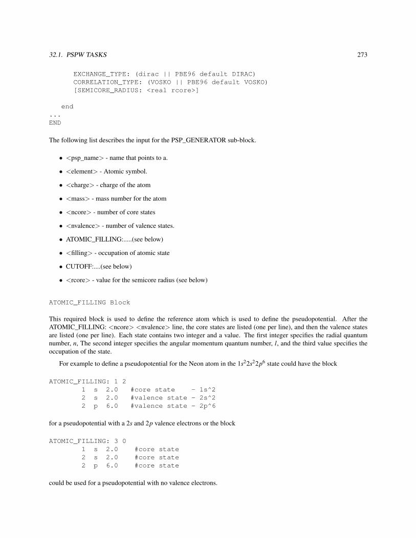
32.1. PSPW TASKS 273
EXCHANGE_TYPE: (dirac || PBE96 default DIRAC)CORRELATION_TYPE: (VOSKO || PBE96 default VOSKO)[SEMICORE_RADIUS: <real rcore>]
end...END
The following list describes the input for the PSP_GENERATOR sub-block.
• <psp_name> - name that points to a.
• <element> - Atomic symbol.
• <charge> - charge of the atom
• <mass> - mass number for the atom
• <ncore> - number of core states
• <nvalence> - number of valence states.
• ATOMIC_FILLING:.....(see below)
• <filling> - occupation of atomic state
• CUTOFF:....(see below)
• <rcore> - value for the semicore radius (see below)
ATOMIC_FILLING Block
This required block is used to define the reference atom which is used to define the pseudopotential. After theATOMIC_FILLING: <ncore> <nvalence> line, the core states are listed (one per line), and then the valence statesare listed (one per line). Each state contains two integer and a value. The first integer specifies the radial quantumnumber, n, The second integer specifies the angular momentum quantum number, l, and the third value specifies theoccupation of the state.
For example to define a pseudopotential for the Neon atom in the 1s22s22p6 state could have the block
ATOMIC_FILLING: 1 21 s 2.0 #core state - 1s^22 s 2.0 #valence state - 2s^22 p 6.0 #valence state - 2p^6
for a pseudopotential with a 2s and 2p valence electrons or the block
ATOMIC_FILLING: 3 01 s 2.0 #core state2 s 2.0 #core state2 p 6.0 #core state
could be used for a pseudopotential with no valence electrons.

274 CHAPTER 32. PSEUDOPOTENTIAL PLANE-WAVE DENSITY FUNCTIONAL THEORY (NWPW)
CUTOFF Block
This optional block specifies the cutoff distances used to match the all-electron atom to the pseudopotential atom. ForHamann pseudopotentials rcut(l) defines the distance where the all-electron potential is matched to the pseudopotential,and for Troullier-Martins pseudopotentials rcut(l) defines the distance where the all-electron orbital is matched to thepseudowavefunctions. Thus the definition of the radii depends on the type of pseudopotential. The cutoff radii used inHamann pseudopotentials will be smaller than the cutoff radii used in Troullier-Martins pseudopotentials.
For example to define a softened Hamann pseudopotential for Carbon would be
ATOMIC_FILLING: 1 21 s 2.02 s 2.02 p 2.0
CUTOFF: 2s 0.8p 0.85d 0.85
while a similarly softened Troullier-Marting pseudopotential for Carbon would be
ATOMIC_FILLING: 1 21 s 2.02 s 2.02 p 2.0
CUTOFF: 2s 1.200p 1.275d 1.275
SEMICORE_RADIUS Option
Specifying the SEMICORE_RADIUS option turns on the semicore correction approximation proposed by Louie etal (S.G. Louie, S. Froyen, and M.L. Cohen, Phys. Rev. B, 26, 1738, (1982)). This approximation is known todramatically improve results for systems containing alkali and transition metal atoms.
The implementation in the PSPW module defines the semi-core density, ρsemicore in terms of the core density, ρcore,by using the sixth-order polynomial
ρsemicore(r) ={
ρcore if r ≥ rsemicorec0 + c3r3 + c4r4 + c5r5 + c6r6 if r < rsemicore
(32.2)
This expansion was suggested by Fuchs and Scheffler (M. Fuchs, and M. Scheffler, Comp. Phys. Comm.,119,67(1999)), and is better behaved for taking derivatives (i.e. calculating ionic forces) than the expansion suggested byLouie et al.
32.1.11 WAVEFUNCTION_INITIALIZER
The functionality of this task is now performed automatically. For backward compatibility, we provide a descriptionof the input to this task.

32.1. PSPW TASKS 275
The wavefunction_initializer task is used to generate an initial wavefunction datafile. Input to the WAVEFUNC-TION_INITIALIZER task is contained within the WAVEFUNCTION_INITIALIZER sub-block.
PSPW...WAVEFUNCTION_INITIALIZER
...END...
END
To run a WAVEFUNCTION_INITIALIZER calculation the following directive is used:
TASK PSPW WAVEFUNCTION_INITIALIZER
Listed below is the format of a WAVEFUNCTION_INITIALIZER sub-block.
PSPW...
WAVEFUNCTION_INITIALIZERCELL_NAME: <string cell_name>WAVEFUNCTION_FILENAME: <string wavefunction_name default input_movecs>(RESTRICTED||UNRESTRICTED)if (RESTRICTED)
RESTRICTED_ELECTRONS: <integer restricted electrons>if (UNRESTRICTED)
UP_ELECTRONS: <integer up_electrons>DOWN_ELECTRONS: <integer down_electrons>
END...END
The following list describes the input for the WAVEFUNCTION_INITIALIZER sub-block.
• <cell_name> - name of the simulation_cell named <cell_name>. See section 32.1.1.
• <wavefunction_name> - name that will point to a wavefunction file.
• RESTRICTED - keyword specifying that the calculation is restricted.
• UNRESTRICTED - keyword specifying that the calculation is unrestricted.
• <restricted_electrons> - number of restricted electrons. Not used if an UNRESTRICTED calculation.
• <up_electrons> - number of spin-up electrons. Not used if a RESTRICTED calculation.
• <down_electrons> - number of spin-down electrons. Not used if a RESTRICTED calculation.
Old Style Input (version 3.3) to WAVEFUNCTION_INITIALIZER
For backward compatibility, the input to the WAVEFUNCTION_INITIALIZER sub-block can also be of the form

276 CHAPTER 32. PSEUDOPOTENTIAL PLANE-WAVE DENSITY FUNCTIONAL THEORY (NWPW)
PSPW...
WAVEFUNCTION_INITIALIZERCELL_NAME: <string cell_name>WAVEFUNCTION_FILENAME: <string wavefunction_name default input_movecs>(RESTRICTED||UNRESTRICTED)
[UP_FILLING: <integer up_filling>[0 0 0 0]{<integer kx ky kz> (-2||-1||1||2)}]
[DOWN_FILLING: <integer down_filling>[0 0 0 0]{<integer kx ky kz> (-2||-1||1||2)}]
END...END
where
• <cell_name> - name of the simulation_cell named <cell_name>. See section 32.1.1.
• <wavefunction_name> - name that will point to a wavefunction file.
• RESTRICTED - keyword specifying that the calculation is restricted.
• UNRESTRICTED - keyword specifying that the calculation is unrestricted.
• <up_filling> - number of restricted molecular orbitals if RESTRICTED and number of spin-up molecularorbitals if UNRESTRICTED.
• <down_filling> - number of spin-down molecular orbitals if UNRESTRICTED. Not used if a RESTRICTEDcalculation.
• <kx ky kz> - specifies which planewave is to be filled.
The values for the planewave (−2|| − 1||1||2) are used to represent whether the specified planewave is a cosineor a sine function, in addition random noise can be added to these base functions. That is +1 represents a cosinefunction, and −1 represents a sine function. The +2 and −2 values are used to represent a cosine function withrandom components added and a sine function with random components added respectively.
32.1.12 V_WAVEFUNCTION_INITIALIZER
The functionality of this task is now performed automatically. For backward compatibility, we provide a descriptionof the input to this task.
The v_wavefunction_initializer task is used to generate an initial velocity wavefunction datafile. Input to theV_WAVEFUNCTION_INITIALIZER task is contained within the V_WAVEFUNCTION_INITIALIZER sub-block.
PSPW...V_WAVEFUNCTION_INITIALIZER
...

32.1. PSPW TASKS 277
END...
END
To run a V_WAVEFUNCTION_INITIALIZER calculation the following directive is used:
TASK PSPW WAVEFUNCTION_INITIALIZER
Listed below is the format of a V_WAVEFUNCTION_INITIALIZER sub-block.
PSPW...
V_WAVEFUNCTION_INITIALIZERV_WAVEFUNCTION_FILENAME: <string v_wavefunction_name default input_vmovecs>CELL_NAME: <string cell_name>(RESTRICTED||UNRESTRICTED)UP_FILLING: <integer up_filling>DOWN_FILLING: <integer down_filling>
END...END
The following list describes the input for the V_WAVEFUNCTION_INITIALIZER sub-block.
• <cell_name> - name of the simulation_cell named <cell_name>. See section 32.1.1.
• <wavefunction_name> - name that will point to a velocity wavefunction file.
• RESTRICTED - keyword specifying that the calculation is restricted.
• UNRESTRICTED - keyword specifying that the calculation is unrestricted.
• <up_filling> - number of restricted velocity molecular orbitals if RESTRICTED and number of spin-up velocitymolecular orbitals if UNRESTRICTED.
• <down_filling> - number of spin-down velocity molecular orbitals if UNRESTRICTED. Not used if a RE-STRICTED calculation.
32.1.13 WAVEFUNCTION_EXPANDER
The functionality of this task is now performed automatically. For backward compatibility, we provide a descriptionof the input to this task.
The wavefunction_expander task is used to convert a new wavefunction file that spans a larger grid space froman old wavefunction file. Input to the WAVEFUNCTION_EXPANDER task is contained within the WAVEFUNC-TION_EXPANDER sub-block.
PSPW...WAVEFUNCTION_EXPANDER
...END...
END
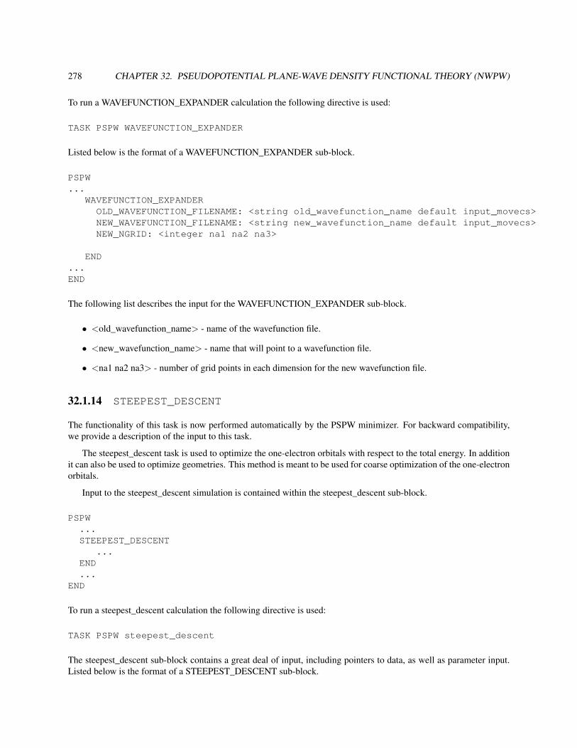
278 CHAPTER 32. PSEUDOPOTENTIAL PLANE-WAVE DENSITY FUNCTIONAL THEORY (NWPW)
To run a WAVEFUNCTION_EXPANDER calculation the following directive is used:
TASK PSPW WAVEFUNCTION_EXPANDER
Listed below is the format of a WAVEFUNCTION_EXPANDER sub-block.
PSPW...
WAVEFUNCTION_EXPANDEROLD_WAVEFUNCTION_FILENAME: <string old_wavefunction_name default input_movecs>NEW_WAVEFUNCTION_FILENAME: <string new_wavefunction_name default input_movecs>NEW_NGRID: <integer na1 na2 na3>
END...END
The following list describes the input for the WAVEFUNCTION_EXPANDER sub-block.
• <old_wavefunction_name> - name of the wavefunction file.
• <new_wavefunction_name> - name that will point to a wavefunction file.
• <na1 na2 na3> - number of grid points in each dimension for the new wavefunction file.
32.1.14 STEEPEST_DESCENT
The functionality of this task is now performed automatically by the PSPW minimizer. For backward compatibility,we provide a description of the input to this task.
The steepest_descent task is used to optimize the one-electron orbitals with respect to the total energy. In additionit can also be used to optimize geometries. This method is meant to be used for coarse optimization of the one-electronorbitals.
Input to the steepest_descent simulation is contained within the steepest_descent sub-block.
PSPW...STEEPEST_DESCENT
...END...
END
To run a steepest_descent calculation the following directive is used:
TASK PSPW steepest_descent
The steepest_descent sub-block contains a great deal of input, including pointers to data, as well as parameter input.Listed below is the format of a STEEPEST_DESCENT sub-block.

32.1. PSPW TASKS 279
PSPW...
STEEPEST_DESCENTCELL_NAME <string cell_name>[GEOMETRY_OPTIMIZE]INPUT_WAVEFUNCTION_FILENAME <string input_wavefunctions default input_movecs>OUTPUT_WAVEFUNCTION_FILENAME <string output_wavefunctions default input_movecs>FAKE_MASS <real fake_mass default 400000.0>TIME_STEP <real time_step default 5.8>LOOP <integer inner_iteration outer_iteration default 10 1>TOLERANCES <real tole tolc tolr default 1.0d-9 1.0d-9 1.0d-4>ENERGY_CUTOFF <real ecut default (see input desciption)>WAVEFUNCTION_CUTOFF <real wcut default (see input description)>EWALD_NCUT <integer ncut default 1>EWALD_RCUT <real rcut default (see input description)>XC (Vosko || LDA || PBE96 || revPBE || HF || PBE0 || revPBE0 ||
LDA-SIC || LDA-SIC/2 || LDA-0.4SIC || LDA-SIC/4 || LDA-0.2SIC ||PBE96-SIC || PBE96-SIC/2 || PBE96-0.4SIC || PBE96-SIC/4 || PBE96-0.2SIC ||revPBE-SIC || revPBE-SIC/2 || revPBE-0.4SIC || revPBE-SIC/4 || revPBE-0.2SIC ||default Vosko)
[MULLIKEN]
END...
END
The following list describes the input for the STEEPEST_DESCENT sub-block.
• <cell_name> - name of the simulation_cell named <cell_name>. See section 32.1.1.
• GEOMETRY_OPTIMIZE - optional keyword which if specified turns on geometry optimization.
• <input_wavefunctions> - name of the file containing one-electron orbitals
• <output_wavefunctions> - name of the file tha will contain the one-electron orbitals at the end of the run.
• <fake_mass> - value for the electronic fake mass (µ).
• <time_step> - value for the time step (∆t).
• <inner_iteration> - number of iterations between the printing out of energies and tolerances
• <outer_iteration> - number of outer iterations
• <tole> - value for the energy tolerance.
• <tolc> - value for the one-electron orbital tolerance.
• <tolr> - value for the ion position tolerance.
• <ecut> - value for the cutoff energy used to define the density. Default is set to be the maximum value that willfit within the simulation_cell <cell_name>.
• <wcut> - value for the cutoff energy used to define the one-electron orbitals. Default is set to be the maximumvalue that will fit within the simulation_cell <cell_name>.

280 CHAPTER 32. PSEUDOPOTENTIAL PLANE-WAVE DENSITY FUNCTIONAL THEORY (NWPW)
• <ncut> - value for the number of unit cells to sum over (in each direction) for the real space part of the Ewaldsummation. Note Ewald summation is only used if the simulation_cell is periodic.
• <rcut> - value for the cutoff radius used in the Ewald summation. Note Ewald summation is only used if thesimulation_cell is periodic.Default set to be MIN(|~ai|)
π, i = 1,2,3.
• (Vosko || PBE96 || revPBE || ...) - Choose between Vosko et al’s LDA parameterization or the orginal andrevised Perdew, Burke, and Ernzerhof GGA functional. In addition, several hybrid options.
• MULLIKEN - optional keyword which if specified causes a Mulliken analysis to be performed at the end of thesimulation.
32.2 Band Tasks
All input to the Band Tasks is contained within the compound NWPW block,
NWPW...
END
To perform an actual calculation a TASK Band directive is used (Section 5.10).
TASK Band
Once a user has specified a geometry, the Band module can be invoked with no input directives (defaults invokedthroughout). There are sub-directives which allow for customized application; those currently provided as options forthe Band module are:
NWPWCELL_NAME <string cell_name default ’cell_default’>ZONE_NAME <string zone_name default ’zone_default’>INPUT_WAVEFUNCTION_FILENAME <string input_wavefunctions default input_movecs>OUTPUT_WAVEFUNCTION_FILENAME <string output_wavefunctions default input_movecs>FAKE_MASS <real fake_mass default 400000.0>TIME_STEP <real time_step default 5.8>LOOP <integer inner_iteration outer_iteration default 10 100>TOLERANCES <real tole tolc default 1.0e-7 1.0e-7>CUTOFF <real cutoff>ENERGY_CUTOFF <real ecut default (see input description)>WAVEFUNCTION_CUTOFF <real wcut default (see input description)>EWALD_NCUT <integer ncut default 1>]EWALD_RCUT <real rcut default (see input description)>XC (Vosko || PBE96 || revPBE default Vosko)DFT||ODFT||RESTRICTED||UNRESTRICTEDMULT <integer mult default 1>CGLMBFGSSCF [Anderson|| simple || Broyden]
[CG || RMM-DIIS]

32.2. BAND TASKS 281
[density || potential][ALPHA real alpha default 0.25][ITERATIONS integer inner_iterations default 5][OUTER_ITERATIONS integer outer_iterations default 0]
SIMULATION_CELL ... (see input description) ENDBRILLOUIN_ZONE ... (see input description) ENDMONKHORST-PACK <real n1 n2 n3 default 1 1 1>
BAND_DPLOT ... (see input description) END
MAPPING <integer mapping default 1>SMEAR <sigma default 0.001> [TEMPERATURE <temperature>] [FERMI || GAUSSIAN default FERMI]
[ORBITALS <integer orbitals default 4>]
END
The following list describes these keywords.
• <cell_name> - name of the simulation_cell named <cell_name>. See section 32.1.1.
• <input_wavefunctions> - name of the file containing one-electron orbitals
• <output_wavefunctions> - name that will point to file containing the one-electron orbitals at the end of the run.
• <fake_mass> - value for the electronic fake mass (µ). This parameter is not presently used in a conjugategradient simulation
• <time_step> - value for the time step (∆t). This parameter is not presently used in a conjugate gradient simu-lation.
• <inner_iteration> - number of iterations between the printing out of energies and tolerances
• <outer_iteration> - number of outer iterations
• <tole> - value for the energy tolerance.
• <tolc> - value for the one-electron orbital tolerance.
• <cutoff> - value for the cutoff energy used to define the wavefunction. In addition using the CUTOFF keywordautomatically sets the cutoff energy for the density to be twice the wavefunction cutoff.
• <ecut> - value for the cutoff energy used to define the density. Default is set to be the maximum value that willfit within the simulation_cell <cell_name>.
• <wcut> - value for the cutoff energy used to define the one-electron orbitals. Default is set to be the maximumvalue that will fix within the simulation_cell <cell_name>.
• <ncut> - value for the number of unit cells to sum over (in each direction) for the real space part of the Ewaldsummation. Note Ewald summation is only used if the simulation_cell is periodic.
• <rcut> - value for the cutoff radius used in the Ewald summation. Note Ewald summation is only used if thesimulation_cell is periodic.Default set to be MIN(|~ai|)
π, i = 1,2,3.

282 CHAPTER 32. PSEUDOPOTENTIAL PLANE-WAVE DENSITY FUNCTIONAL THEORY (NWPW)
• (Vosko || PBE96 || revPBE) - Choose between Vosko et al’s LDA parameterization or the orginal and revisedPerdew, Burke, and Ernzerhof GGA functional.
• SIMULATION_CELL (see section 32.1.1)
• BRILLOUIN_ZONE (see section 32.2.1)
• MONKHORST-PACK - Alternatively, the MONKHORST-PACK keyword can be used to enter a MONKHORST-PACK sampling of the Brillouin zone.
• <smear> - value for smearing broadending
• <temperature> - same as smear but in units of K.
• CG - optional keyword which sets the minimizer to 1
• LMBFGS - optional keyword which sets the minimizer to 2
• SCF - optional keyword which sets the minimizer to be a band by band minimizer. Several options are availablefor setting the density or potential mixing, and the type of Kohn-Sham minimizer.
32.2.1 Brillouin Zone
To supply the special points of the Brillouin zone, the user defines a brillouin_zone sub-block within the NWPWblock. Listed below is the format of a brillouin_zone sub-block.
NWPW...
BRILLOUIN_ZONEZONE_NAME <string name default ’zone_default’>(KVECTOR <real k1 k2 k3 no default> <real weight default (see input description)>...)
END...END
The user enters the special points and weights of the Brillouin zone. The following list describes the input in detail.
• <name> - user-supplied name for the simulation block.
• <k1 k2 k3> - user-supplied values for a special point in the Brillouin zone.
• <weight> - user-supplied weight. Default is to set the weight so that the sum of all the weights for the enteredspecial points adds up to unity.
32.2.2 BAND_DPLOT
The BAND BAND_DPLOT task is used to generate plots of various types of electron densities (or orbitals) of a crystal.The electron density is calculated on the specified set of grid points from a Band calculation. The output file generatedis in the Gaussian Cube format. Input to the BAND_DPLOT task is contained within the BAND_DPLOT sub-block.
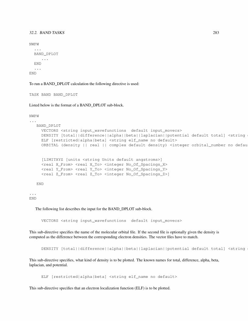
32.2. BAND TASKS 283
NWPW...BAND_DPLOT
...END...
END
To run a BAND_DPLOT calculation the following directive is used:
TASK BAND BAND_DPLOT
Listed below is the format of a BAND_DPLOT sub-block.
NWPW...
BAND_DPLOTVECTORS <string input_wavefunctions default input_movecs>DENSITY [total||difference||alpha||beta||laplacian||potential default total] <string density_name no default>ELF [restricted|alpha|beta] <string elf_name no default>ORBITAL (density || real || complex default density) <integer orbital_number no default> <integer brillion_number default 1> <string orbital_name no default>
[LIMITXYZ [units <string Units default angstroms>]<real X_From> <real X_To> <integer No_Of_Spacings_X><real Y_From> <real Y_To> <integer No_Of_Spacings_Y><real Z_From> <real Z_To> <integer No_Of_Spacings_Z>]
END
...END
The following list describes the input for the BAND_DPLOT sub-block.
VECTORS <string input_wavefunctions default input_movecs>
This sub-directive specifies the name of the molecular orbital file. If the second file is optionally given the density iscomputed as the difference between the corresponding electron densities. The vector files have to match.
DENSITY [total||difference||alpha||beta||laplacian||potential default total] <string density_name no default>
This sub-directive specifies, what kind of density is to be plotted. The known names for total, difference, alpha, beta,laplacian, and potential.
ELF [restricted|alpha|beta] <string elf_name no default>
This sub-directive specifies that an electron localization function (ELF) is to be plotted.
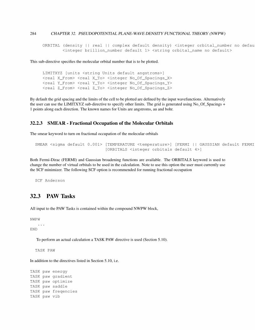
284 CHAPTER 32. PSEUDOPOTENTIAL PLANE-WAVE DENSITY FUNCTIONAL THEORY (NWPW)
ORBITAL (density || real || complex default density) <integer orbital_number no default> \<integer brillion_number default 1> <string orbital_name no default>
This sub-directive specifies the molecular orbital number that is to be plotted.
LIMITXYZ [units <string Units default angstroms>]<real X_From> <real X_To> <integer No_Of_Spacings_X><real Y_From> <real Y_To> <integer No_Of_Spacings_Y><real Z_From> <real Z_To> <integer No_Of_Spacings_Z>
By default the grid spacing and the limits of the cell to be plotted are defined by the input wavefunctions. Alternativelythe user can use the LIMITXYZ sub-directive to specify other limits. The grid is generated using No_Of_Spacings +1 points along each direction. The known names for Units are angstroms, au and bohr.
32.2.3 SMEAR - Fractional Occupation of the Molecular Orbitals
The smear keyword to turn on fractional occupation of the molecular orbitals
SMEAR <sigma default 0.001> [TEMPERATURE <temperature>] [FERMI || GAUSSIAN default FERMI][ORBITALS <integer orbitals default 4>]
Both Fermi-Dirac (FERMI) and Gaussian broadening functions are available. The ORBITALS keyword is used tochange the number of virtual orbitals to be used in the calculation. Note to use this option the user must currently usethe SCF minimizer. The following SCF option is recommended for running fractional occupation
SCF Anderson
32.3 PAW Tasks
All input to the PAW Tasks is contained within the compound NWPW block,
NWPW...
END
To perform an actual calculation a TASK PAW directive is used (Section 5.10).
TASK PAW
In addition to the directives listed in Section 5.10, i.e.
TASK paw energyTASK paw gradientTASK paw optimizeTASK paw saddleTASK paw freqenciesTASK paw vib

32.3. PAW TASKS 285
there are additional directives that are specific to the PSPW module, which are:
TASK PAW [Car-Parrinello ||steepest_descent ]
Once a user has specified a geometry, the PAW module can be invoked with no input directives (defaults invokedthroughout). There are sub-directives which allow for customized application; those currently provided as options forthe PAW module are:
NWPWCELL_NAME <string cell_name default ’cell_default’>[GEOMETRY_OPTIMIZE]INPUT_WAVEFUNCTION_FILENAME <string input_wavefunctions default input_movecs>OUTPUT_WAVEFUNCTION_FILENAME <string output_wavefunctions default input_movecs>FAKE_MASS <real fake_mass default 400000.0>TIME_STEP <real time_step default 5.8>LOOP <integer inner_iteration outer_iteration default 10 100>TOLERANCES <real tole tolc default 1.0e-7 1.0e-7>CUTOFF <real cutoff>ENERGY_CUTOFF <real ecut default (see input description)>WAVEFUNCTION_CUTOFF <real wcut default (see input description)>EWALD_NCUT <integer ncut default 1>]EWALD_RCUT <real rcut default (see input description)>XC (Vosko || PBE96 || revPBE default Vosko)DFT||ODFT||RESTRICTED||UNRESTRICTEDMULT <integer mult default 1>INTEGRATE_MULT_L <integer imult default 1>
SIMULATION_CELL ... (see input description) ENDCAR-PARRINELLO ... (see input description) END
MAPPING <integer mapping default 1>END
END
The following list describes these keywords.
• <cell_name> - name of the the simulation_cell named <cell_name>. The current version of PAW only acceptsperiodic unit cells. See section 32.1.1.
• GEOMETRY_OPTIMIZE - optional keyword which if specified turns on geometry optimization.
• <input_wavefunctions> - name of the file containing one-electron orbitals
• <output_wavefunctions> - name of the file that will contain the one-electron orbitals at the end of the run.
• <fake_mass> - value for the electronic fake mass (µ). This parameter is not presently used in a conjugategradient simulation
• <time_step> - value for the time step (∆t). This parameter is not presently used in a conjugate gradient simu-lation.

286 CHAPTER 32. PSEUDOPOTENTIAL PLANE-WAVE DENSITY FUNCTIONAL THEORY (NWPW)
• <inner_iteration> - number of iterations between the printing out of energies and tolerances
• <outer_iteration> - number of outer iterations
• <tole> - value for the energy tolerance.
• <tolc> - value for the one-electron orbital tolerance.
• <cutoff> - value for the cutoff energy used to define the wavefunction. In addition using the CUTOFF keywordautomatically sets the cutoff energy for the density to be twice the wavefunction cutoff.
• <ecut> - value for the cutoff energy used to define the density. Default is set to be the maximum value that willfit within the simulation_cell <cell_name>.
• <wcut> - value for the cutoff energy used to define the one-electron orbitals. Default is set to be the maximumvalue that will fix within the simulation_cell <cell_name>.
• <ncut> - value for the number of unit cells to sum over (in each direction) for the real space part of the smoothcompensation summation.
• <rcut> - value for the cutoff radius used in the smooth compensation summation.Default set to be MIN(|~ai|)
π, i = 1,2,3.
• (Vosko || PBE96 || revPBE) - Choose between Vosko et al’s LDA parameterization or the orginal and revisedPerdew, Burke, and Ernzerhof GGA functional.
• MULT - optional keyword which if specified allows the user to define the spin multiplicity of the system
• INTEGRATE_MULT_L - optional keyword which if specified allows the user to define the angular XC integra-tion of the augmented region
• SIMULATION_CELL (see section 32.1.1)
• CAR-PARRINELLO(see section 32.1.7)
• <mapping> - for a value of 1 slab FFT is used, for a value of 2 a 2d-hilbert FFT is used.
32.4 Pseudopotential and PAW basis Libraries
A library of pseudopotentials used by PSPW and BAND is currently available in the directory$NWCHEM_TOP/src/nwpw/libraryps/pspw_default
The elements listed in the following table are present:
H He------- ------------------Li Be B C N O F Ne------- -------------------Na Mg Al Si P S Cl Ar-------------------------------------------------------K Ca Sc Ti V Cr Mn Fe Co Ni Cu Zn Ga Ge As Se Br Kr-------------------------------------------------------Rb Sr Y Zr Nb Mo Tc Ru Rh Pd Ag Cd In Sn Sb Te I Xe-------------------------------------------------------

32.4. PSEUDOPOTENTIAL AND PAW BASIS LIBRARIES 287
Cs Ba La Hf Ta W Re Os Ir Pt Au Hg Tl Pb Bi Po At Rn-------------------------------------------------------Fr Ra .-----------------
------------------------------------------. . . . . . Gd . . . . . . .------------------------------------------. . U . Pu . . . . . . . . .------------------------------------------
The pseudopotential libraries are continually being tested and added. Also, the PSPW program can read in pseudopo-tentials in CPI and TETER format generated with pseudopotential generation programs such as the OPIUM packageof Rappe et al. The user can request additional pseudopotentials from Eric J. Bylaska at ([email protected]).
Similarly, a library of PAW basis used by PAW is currently available in the directory$NWCHEM_TOP/src/nwpw/libraryps/paw_default
H He------- -----------------Li Be B C N O F Ne------- ------------------Na Mg Al Si P S Cl Ar------------------------------------------------------K Ca Sc Ti V Cr Mn Fe Co Ni Cu Zn Ga Ge As Se Br Kr------------------------------------------------------. . . . . . . . . . . . . . . . . .------------------------------------------------------. . . . . . . . . . . . . . . . . .------------------------------------------------------. . .-----------------
------------------------------------------. . . . . . . . . . . . . .------------------------------------------. . . . . . . . . . . . . .------------------------------------------
Currently there are not very many elements available for PAW. However, the user can request additional basis setsfrom Eric J. Bylaska at ([email protected]).
A preliminary implementation of the HGH pseudopotentials (Hartwigsen, Goedecker, and Hutter) has been imple-mented into the PSPW module. To access the pseudopotentials the pseudopotentials input block is used. For example,to redirect the code to use HGH pseudopotentials for carbon and hydrogen, the following input would be used.
nwpw...

288 CHAPTER 32. PSEUDOPOTENTIAL PLANE-WAVE DENSITY FUNCTIONAL THEORY (NWPW)
pseudopotentialsC library HGH_LDAH library HGH_LDAend...
end
The implementation of HGH pseudopotentials is rather limited in this release. HGH pseudopotentials cannot be usedto optimize unit cells, and they do not work with the MULLIKEN option. They also have not yet been implementedinto the BAND structure code.
To read in pseudopotentials in CPI format the following input would be used.
nwpw...pseudopotentialsC CPI c.cpiH CPI h.cpiend...
end
In order for the program to recognize the CPI format the CPI files, e.g. c.cpi have to be prepended with the “<CPI>”keyword.
To read in pseudopotentials in TETER format the following input would be used.
nwpw...pseudopotentialsC TETER c.teterH TETER h.teterend...
end
In order for the program to recognize the TETER format the TETER files, e.g. c.teter have to be prepended with the“<TETER>” keyword.
If you wish to redirect the code to a different directory other than the default one, you need to set the environmentalvariable NWCHEM_NWPW_LIBRARY to the new location of the libraryps directory.
32.5 NWPW RTDB Entries and DataFiles
Input to the PSPW and Band modules are contained in both the RTDB and datafiles. The RTDB is used to store inputthat the user will need to directly specify. Input of this kind includes ion positions, ion velocities, and simulationcell parameters. The datafiles are used to store input, such the one-electron orbitals, one-electron orbital velocities,formatted pseudopotentials, and one-dimensional pseudopotentials, that the user will in most cases run a program togenerate.

32.5. NWPW RTDB ENTRIES AND DATAFILES 289
32.5.1 Ion Positions
The positions of the ions are stored in the default geometry structure in the RTDB and must be specified using theGEOMETRY directive.
32.5.2 Ion Velocities
The velocities of the ions are stored in the default geometry structure in the RTDB, and must be specified using theGEOMETRY directive.
32.5.3 Wavefunction Datafile
The one-electron orbitals are stored in a wavefunction datafile. This is a binary file and cannot be directly edited. Thisdatafile is used by steepest_descent and Car-Parrinello tasks and can be generated using the wavefunction_initializeror wavefunction_expander tasks.
32.5.4 Velocity Wavefunction Datafile
The one-electron orbital velocities are stored in a velocity wavefunction datafile. This is a binary file and cannot be di-rectly edited. This datafile is used by the Car-Parrinello task and can be generated using the v_wavefunction_initializertask.
32.5.5 Formatted Pseudopotential Datafile
The pseudopotentials in Kleinman-Bylander form expanded on a simulation cell (3d grid) are stored in a formattedpseudopotential datafile. This is a binary file and cannot be directly edited. This datafile is used by steepest_descentand Car-Parrinello tasks and can be generated using the pseudopotential_formatter task.
32.5.6 One-Dimensional Pseudopotential Datafile
The one-dimensional pseudopotentials are stored in a one-dimensional pseudopotential file. This is an ASCII file andcan be directly edited with a text editor. However, the user will usually use the psp_generator task to generate thisdatafile.
The data stored in the one-dimensional pseudopotential file is
character*2 element :: element nameinteger charge :: valence charge of ionreal mass :: mass of ioninteger lmax :: maximum angular componentreal rcut(lmax) :: cutoff radii used to define pseudopotentialsinteger nr :: number of points in the radial gridreal dr :: linear spacing of the radial gridreal r(nr) :: one-dimensional radial gridreal Vpsp(nr,lmax) :: one-dimensional pseudopotentialsreal psi(nr,lmax) :: one-dimensional pseudowavefunctionsreal r_semicore :: semicore radius

290 CHAPTER 32. PSEUDOPOTENTIAL PLANE-WAVE DENSITY FUNCTIONAL THEORY (NWPW)
real rho_semicore(nr) :: semicore density
and the format of it is:
[line 1: ] element[line 2: ] charge mass lmax[line 3: ] (rcut(l), l=1,lmax)[line 4: ] nr dr[line 5: ] r(1) (Vpsp(1,l), l=1,lmax)[line 6: ] ....[line nr+4: ] r(nr) (Vpsp(nr,l), l=1,lmax)[line nr+5: ] r(1) (psi(1,l), l=1,lmax)[line nr+6: ] ....[line 2*nr+4:] r(nr) (psi(nr,l), l=1,lmax)[line 2*nr+5:] r_semicoreif (r_semicore read) then[line 2*nr+6:] r(1) rho_semicore(1)[line 2*nr+7:] ....[line 3*nr+5:] r(nr) rho_semicore(nr)end if
32.5.7 PSPW Car-Parrinello Output Datafiles
XYZ motion file
Data file that stores ion positions and velocities as a function of time in XYZ format.
[line 1: ] n_ion[line 2: ]do ii=1,n_ion[line 2+ii: ] atom_name(ii), x(ii),y(ii),z(ii),vx(ii),vy(ii),vz(ii)end do[line n_ion+3 ] n_nion
do ii=1,n_ion[line n_ion+3+ii: ] atom_name(ii), x(ii),y(ii),z(ii), vx(ii),vy(ii),vz(ii)end do[line 2*n_ion+4: ] ....
ION_MOTION motion file
Datafile that stores ion positions and velocities as a function of time
[line 1: ] it_out, n_ion, omega[line 2: ] timedo ii=1,n_ion[line 2+ii: ] x(ii),y(ii),z(ii), vx(ii),vy(ii),vz(ii)end do[line n_ion+3 ] time

32.6. CAR-PARRINELLO SCHEME FOR AB INITIO MOLECULAR DYNAMICS 291
dodo ii=1,n_ion[line n_ion+3+ii: ] x(ii),y(ii),z(ii), vx(ii),vy(ii),vz(ii)end do[line 2*n_ion+4: ] ....
EMOTION motion file
Datafile that store energies as a function of time
[line 1: ] time, E1,E2,E3,E4,E5,E6,E7,E8, (E9,E10, if Nose-Hoover)[line 2: ] ...
HMOTION motion file
Datafile that stores the rotation matrix as a function of time.
[line 1: ] time[line 2: ] ms,ne(ms),ne(ms)do i=1,ne(ms)[line 2+i: ] (hml(i,j), j=1,ne(ms)end do[line 3+ne(ms): ] time[line 4+ne(ms): ] ....
EIGMOTION motion file
Datafile that stores the eigenvalues for the one-electron orbitals as a function of time.
[line 1: ] time, (eig(i), i=1,number_orbitals)[line 2: ] ...
OMOTION motion file
Datafile that stores a reduced representation of the one-electron orbitals. To be used with a molecular orbital viewerthat will be ported to NWChem in the near future.
32.6 Car-Parrinello Scheme for Ab Initio Molecular Dynamics
Car and Parrinello developed a unified scheme for doing ab initio molecular dynamics by combining the motion of theion cores and a fictitious motion for the Kohn-Sham orbitals of density-functional theory (R. Car and M. Parrinello,Phys. Rev. Lett. 55, 2471, (1985)). At the heart of this method they introduced a fictitious kinetic energy functionalfor the Kohn-Sham orbitals.

292 CHAPTER 32. PSEUDOPOTENTIAL PLANE-WAVE DENSITY FUNCTIONAL THEORY (NWPW)
KE({ψi,σ(~r)}) =occ
∑i,σ
∫d~r µ |ψi,σ(~r)|2 (32.3)
Given this kinetic energy the constrained equations of motion are found by taking the first variation of the auxiliaryLagrangian.
L =occ
∑i,σ
∫d~r µ |ψi,σ(~r)|2 +
12 ∑
IMI
∣∣∣~RI
∣∣∣2−E[{ψi,σ(~r)} ,
{~RI
}]+∑
i j,σΛi j,σ
(∫d~r ψ
∗i,σ(~r)ψ j,σ(~r)−δi j,σ
)(32.4)
Which generates a dynamics for the wavefunctions ψi,σ(~r) and atoms positions ~RI through the constrained equationsof motion:
µψi,σ(~r, t) = − δEδψ∗i,σ (~r, t)
+∑j
Λi j,σψ j,σ (~r, t) (32.5)
MI~RI = − ∂E∂~RI
(32.6)
where µ is the fictitious mass for the electronic degrees of freedom and MI are the ionic masses. The adjustable pa-rameter µ is used to describe the relative rate at which the wavefunctions change with time. Λi j,σ are the Lagrangianmultipliers for the orthonormalization of the single-particle orbitals ψi,σ(~r). They are defined by the orthonormaliza-tion constraint conditions and can be rigorously found. However, the equations of motion for the Lagrange multipliersdepend on the specific algorithm used to integrate Eqs. 32.5-32.6.
For this method to give ionic motions that are physically meaningful the kinetic energy of the Kohn-Sham orbitalsmust be relatively small when compared to the kinetic energy of the ions. There are two ways where this criterion canfail. First, the numerical integrations for the Car-Parrinello equations of motion can often lead to large relative valuesof the kinetic energy of the Kohn-Sham orbitals relative to the kinetic energy of the ions. This kind of failure is easilyfixed by requiring a more accurate numerical integration, i.e. use a smaller time step for the numerical integration.Second, during the motion of the system a the ions can be in locations where there is an Kohn-Sham orbital levelcrossing, i.e. the density-functional energy can have two states that are nearly degenerate. This kind of failure oftenoccurs in the study of chemical reactions. This kind of failure is not easily fixed and requires the use of a moresophisticated density-functional energy that accounts for low-lying excited electronic states.
32.6.1 Verlet Algorithm for Integration
Eqs. 32.5-32.6 integrated using the Verlet algorithm results in
ψt+∆ti,σ ← 2ψ
ti,σ−ψ
t−∆ti,σ +
(∆t)2
µ
[δE
δψ∗i,σ+∑
jψ j,σΛ ji,σ
]t
(32.7)

32.6. CAR-PARRINELLO SCHEME FOR AB INITIO MOLECULAR DYNAMICS 293
~Rt+∆tI ← 2~Rt
I−~Rt−∆tI +
(∆t)2
MI
∂E∂~RI
(32.8)
In this molecular dynamic procedure we have to know variational derivative δEδψ∗i,σ
and the matrix Λi j,σ. The
variational derivative δEδψ∗i,σ
can be analytically found and is
δEδψ∗i,σ
= −12
∇2ψi,σ(~r)
+∫
d~r′Wext(~r,~r′)ψi,σ(~r′)
+∫
d~r′n(~r′)
|~r−~r′|ψi,σ(~r)
+ µσxc(~r)ψi,σ(~r)
≡ Hψi,σ (32.9)
To find the matrix Λi j,σ we impose the orthonormality constraint on ψt+∆ti,σ to obtain a matrix Riccatti equation, and
then Riccatti equation is solved by an iterative solution
32.6.2 Constant Temperature Simulations: Nose-Hoover Thermostats
Nose-Hoover Thermostats for the electrons and ions can also be added to the Car-Parrinello simulation. In this typeof simulation thermostats variables xe and xR are added to the simulation by adding the auxiliary energy functionals tothe total energy.
ION_T HERMOSTAT (xR) =12
QRxR +ER0xR (32.10)
ELECT RON_T HERMOSTAT (xe) =12
Qexe +Ee0xe (32.11)
In these equations, the average kinetic energy for the ions is
ER0 =12
f kBT (32.12)
where f is the number of atomic degrees of freedom, kB is Boltzmann’s constant, and T is the desired temperature.Defining the average fictitious kinetic energy of the electrons is not as straightforward. Blöchl and Parrinello (P.E.Blöchl and M. Parrinello, Phys. Rev. B, 45, 9413, (1992)) have suggested the following formula for determining theaverage fictitious kinetic energy
Ee0 = 4kBTµM ∑
i< ψi|−
12
∇2|ψi > (32.13)
where µ is the fictitious electronic mass, M is average mass of one atom, and ∑i < ψi|− 12 ∇2|ψi > is the kinetic energy
of the electrons.
Blöchl and Parrinello suggested that the choice of mass parameters, Qe, and QR should be made such that the periodof oscillating thermostats should be chosen larger than the typical time scale for the dynamical events of interest but

294 CHAPTER 32. PSEUDOPOTENTIAL PLANE-WAVE DENSITY FUNCTIONAL THEORY (NWPW)
shorter than the simulation time.
Pion = 2π
√QR
4ER0(32.14)
Pelectron = 2π
√Qe
4Ee0(32.15)
where Pion and Pelectron are the periods of oscillation for the ionic and fictitious electronic thermostats.
In simulated annealing simulations the electronic and ionic Temperatures are scaled according to an exponentialcooling schedule,
Te(t) = T 0e exp−
tτe (32.16)
Tionic(t) = T 0ionic exp−
tτionic (32.17)
where T 0e and T 0
ionic are the initial temperatures, and τe and τionic are the cooling rates in atomic units.
32.7 PSPW Tutorial 1: Minimizing the geometry for a C2 molecule
In this section we show how use the PSPW module to optimize the geometry for a C2 molecule at the PBE96 levels.
In the following example we show the input needed to optimize the geometry for a C2 molecule at the LDA level.In this example, default pseudopotentials from the pseudopotential library are used for C, the boundary condition isfree-space, the exchange correlation functional is PBE96, The boundary condition is free-space, and the simulationcell cell is aperiodic and cubic with a side length of 10.0 Angstroms and has 40 grid points in each direction (cutoffenergy is 44 Ry).
start c2_pspw_pbe96title "C2 restricted singlet dimer optimization - PBE96/44Ry"
geometryC -0.62 0.0 0.0C 0.62 0.0 0.0end
pspwsimulation_cell units angstroms
boundary_conditions aperiodicSC 10.0ngrid 40 40 40
endxc pbe96
endset nwpw:minimizer 2task pspw optimize
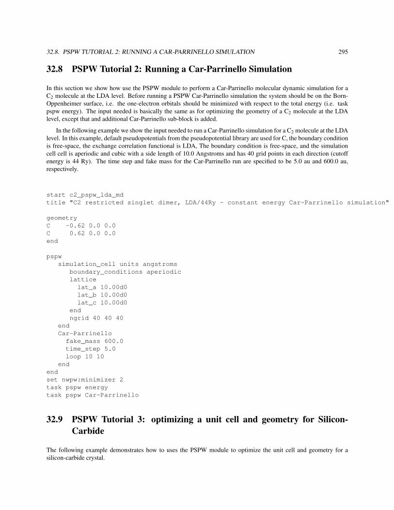
32.8. PSPW TUTORIAL 2: RUNNING A CAR-PARRINELLO SIMULATION 295
32.8 PSPW Tutorial 2: Running a Car-Parrinello Simulation
In this section we show how use the PSPW module to perform a Car-Parrinello molecular dynamic simulation for aC2 molecule at the LDA level. Before running a PSPW Car-Parrinello simulation the system should be on the Born-Oppenheimer surface, i.e. the one-electron orbitals should be minimized with respect to the total energy (i.e. taskpspw energy). The input needed is basically the same as for optimizing the geometry of a C2 molecule at the LDAlevel, except that and additional Car-Parrinello sub-block is added.
In the following example we show the input needed to run a Car-Parrinello simulation for a C2 molecule at the LDAlevel. In this example, default pseudopotentials from the pseudopotential library are used for C, the boundary conditionis free-space, the exchange correlation functional is LDA, The boundary condition is free-space, and the simulationcell cell is aperiodic and cubic with a side length of 10.0 Angstroms and has 40 grid points in each direction (cutoffenergy is 44 Ry). The time step and fake mass for the Car-Parrinello run are specified to be 5.0 au and 600.0 au,respectively.
start c2_pspw_lda_mdtitle "C2 restricted singlet dimer, LDA/44Ry - constant energy Car-Parrinello simulation"
geometryC -0.62 0.0 0.0C 0.62 0.0 0.0end
pspwsimulation_cell units angstroms
boundary_conditions aperiodiclattice
lat_a 10.00d0lat_b 10.00d0lat_c 10.00d0
endngrid 40 40 40
endCar-Parrinello
fake_mass 600.0time_step 5.0loop 10 10
endendset nwpw:minimizer 2task pspw energytask pspw Car-Parrinello
32.9 PSPW Tutorial 3: optimizing a unit cell and geometry for Silicon-Carbide
The following example demonstrates how to uses the PSPW module to optimize the unit cell and geometry for asilicon-carbide crystal.

296 CHAPTER 32. PSEUDOPOTENTIAL PLANE-WAVE DENSITY FUNCTIONAL THEORY (NWPW)
title "SiC 8 atom cubic cell - geometry and unit cell optimization"
start SiC
#**** Enter the geometry using fractional coordinates ****geometry units au center noautosym noautoz print
system crystallat_a 8.277d0lat_b 8.277d0lat_c 8.277d0alpha 90.0d0beta 90.0d0gamma 90.0d0
endSi -0.50000d0 -0.50000d0 -0.50000d0Si 0.00000d0 0.00000d0 -0.50000d0Si 0.00000d0 -0.50000d0 0.00000d0Si -0.50000d0 0.00000d0 0.00000d0C -0.25000d0 -0.25000d0 -0.25000d0C 0.25000d0 0.25000d0 -0.25000d0C 0.25000d0 -0.25000d0 0.25000d0C -0.25000d0 0.25000d0 0.25000d0end
#***** setup the nwpw gamma point code ****nwpw
simulation_cellngrid 16 16 16
endewald_ncut 8
endset nwpw:minimizer 2set nwpw:psi_nolattice .true. # turns of unit cell checking for wavefunctions
driverclearmaxiter 40
endset includestress .true. # this option tells driver to optimize the unit cell
task pspw optimize
32.10 PSPW Tutorial 4: QM/MM simulation for CCl4 + 64H2O
In this section we show how use the PSPW module to perform a Car-Parrinello QM/MM simulation for a CCl4molecule in a box of 64 H2O. Before running a PSPW Car-Parrinello simulation the system should be on the Born-Oppenheimer surface, i.e. the one-electron orbitals should be minimized with respect to the total energy (i.e. taskpspw energy).

32.10. PSPW TUTORIAL 4: QM/MM SIMULATION FOR CCL4 + 64H2O 297
In the following example we show the input needed to run a Car-Parrinello QM/MM simulation for a CCl4molecule in a box of 64 H2O. In this example, default pseudopotentials from the pseudopotential library are usedfor C, Cl, Oˆ and Hˆ exchange correlation functional is PBE96, The boundary condition is periodic, and with a sidelength of 23.577 Bohrs and has a cutoff energy is 50 Ry). The time step and fake mass for the Car-Parrinello run arespecified to be 5.0 au and 600.0 au, respectively.
title "CCl4 + water64 QM/MM simulation- 195 atom cell"
memory 1500 mbstart CCl4-water64
#scratch_dir ./perm#permanent_dir ./perm
geometry nocenter noautoz noautosymC 0.7804E-02 -0.2897E-02 0.1420E-02 -0.2910E-07 -0.1055E-07 -0.2001E-07Cl -0.8603E+00 0.1547E+01 0.2556E+00 -0.2910E-07 -0.1055E-07 -0.2001E-07Cl 0.8421E+00 -0.4774E+00 0.1518E+01 -0.2910E-07 -0.1055E-07 -0.2001E-07Cl -0.1167E+01 -0.1279E+01 -0.4592E+00 -0.2910E-07 -0.1055E-07 -0.2001E-07Cl 0.1218E+01 0.1972E+00 -0.1309E+01 -0.2910E-07 -0.1055E-07 -0.2001E-07
O^ 0.1545E+01 -0.3640E+01 -0.2558E+01 0.1675E-03 -0.2134E-03 0.2608E-03H^ 0.6377E+00 -0.4054E+01 -0.2486E+01 -0.8467E-05 -0.6710E-04 -0.1101E-02H^ 0.1860E+01 -0.3690E+01 -0.3506E+01 0.9734E-03 0.1042E-02 0.4566E-03O^ -0.6138E+01 -0.4627E+01 -0.1181E+01 -0.1477E-03 -0.1616E-03 -0.1670E-03H^ -0.7068E+01 -0.4458E+01 -0.8549E+00 -0.6948E-03 -0.5435E-03 -0.1521E-02H^ -0.5628E+01 -0.5133E+01 -0.4858E+00 -0.8855E-03 0.2768E-03 0.6961E-03O^ 0.3808E+01 0.2935E+01 0.2147E+01 -0.6374E-04 0.1081E-03 -0.3184E-04H^ 0.4187E+01 0.2253E+01 0.2772E+01 0.5832E-03 0.5155E-03 0.2134E-04H^ 0.4511E+01 0.3612E+01 0.1926E+01 -0.4943E-03 0.3230E-03 -0.7034E-03O^ -0.6210E+00 -0.5260E+01 -0.2842E+01 0.1727E-03 0.9623E-04 0.8184E-04H^ -0.2750E+00 -0.5523E+01 -0.3742E+01 0.1119E-03 0.7072E-03 -0.1203E-03H^ -0.7042E+00 -0.6073E+01 -0.2266E+01 -0.6331E-03 -0.4150E-03 -0.7442E-03O^ 0.2760E+01 0.2730E+01 -0.4774E+01 -0.1327E-03 0.3354E-03 -0.1366E-03H^ 0.3676E+01 0.2570E+01 -0.5142E+01 -0.5941E-04 0.5145E-03 -0.3057E-04H^ 0.2828E+01 0.2989E+01 -0.3811E+01 -0.2370E-03 0.1001E-02 -0.3029E-03O^ -0.2387E+01 0.5716E+01 0.3965E+01 -0.6296E-04 -0.1405E-04 -0.2853E-04H^ -0.1694E+01 0.5121E+01 0.3558E+01 0.5787E-04 -0.5014E-03 0.9024E-03H^ -0.1939E+01 0.6465E+01 0.4453E+01 -0.2046E-03 0.6948E-04 -0.2150E-04O^ -0.3456E+01 0.5123E+01 -0.2154E+01 -0.3714E-04 -0.1948E-03 0.4699E-05H^ -0.3043E+01 0.4342E+01 -0.2622E+01 -0.1119E-05 -0.3220E-03 0.2734E-03H^ -0.3693E+01 0.5826E+01 -0.2825E+01 -0.2085E-03 -0.4813E-03 -0.2351E-03O^ 0.5940E+00 0.1399E+01 0.3463E+01 -0.1288E-03 -0.9776E-04 -0.1409E-03H^ 0.1245E+01 0.1913E+01 0.2904E+01 -0.3790E-03 -0.4010E-03 -0.6948E-03H^ -0.3201E+00 0.1790E+01 0.3355E+01 -0.1070E-03 0.6148E-04 0.3431E-03O^ 0.4845E+01 0.4936E+01 0.4088E+01 0.2876E-03 -0.2625E-03 -0.7661E-04H^ 0.4098E+01 0.5168E+01 0.3465E+01 -0.1301E-03 -0.5756E-04 0.4909E-03H^ 0.4740E+01 0.3991E+01 0.4397E+01 0.1202E-02 -0.7660E-03 -0.1345E-02O^ -0.7209E+00 0.4285E+01 0.1237E+01 -0.1519E-03 0.6569E-04 0.1096E-03H^ 0.1958E-01 0.4499E+01 0.6000E+00 -0.5731E-04 -0.2919E-03 0.9929E-04H^ -0.1597E+01 0.4541E+01 0.8281E+00 -0.1117E-03 -0.3977E-03 -0.2666E-03O^ 0.3836E+01 0.2390E-01 -0.6670E+00 0.2697E-04 -0.6474E-05 -0.4852E-03H^ 0.4335E+01 -0.5028E+00 0.2166E-01 -0.1127E-02 0.1144E-02 0.1230E-02H^ 0.2962E+01 -0.4225E+00 -0.8598E+00 -0.1721E-03 0.3171E-03 -0.3321E-03O^ -0.7034E+00 -0.2120E+01 -0.3538E+01 0.1292E-03 -0.1072E-03 -0.1333E-03H^ -0.7567E+00 -0.3086E+01 -0.3284E+01 0.5037E-03 -0.2660E-03 -0.6455E-03H^ 0.2369E+00 -0.1894E+01 -0.3793E+01 0.2452E-03 0.6329E-03 0.9344E-03O^ 0.1465E+01 -0.4009E+01 0.4737E+01 0.3828E-03 -0.5067E-04 0.2649E-03H^ 0.4923E+00 -0.3944E+01 0.4958E+01 0.3572E-03 0.1205E-02 -0.2187E-03H^ 0.1582E+01 -0.4544E+01 0.3901E+01 0.1254E-03 -0.4486E-03 0.4761E-03O^ -0.3224E+01 -0.3091E+00 0.1701E+01 -0.2499E-03 -0.2643E-03 -0.1442E-03H^ -0.2950E+01 -0.9626E+00 0.9949E+00 -0.4237E-03 -0.8809E-04 -0.3749E-03H^ -0.3005E+01 0.6188E+00 0.1398E+01 -0.6682E-03 -0.1587E-03 -0.1246E-03O^ 0.5321E+01 0.3728E+01 -0.5992E+01 0.1243E-03 0.1407E-03 0.3011E-04H^ 0.5383E+01 0.3541E+01 -0.5012E+01 0.2175E-03 -0.4499E-04 0.4888E-05H^ 0.5850E+01 0.3045E+01 -0.6496E+01 -0.1043E-03 0.1021E-03 -0.1441E-03O^ -0.3365E+01 -0.2780E+01 0.3200E+01 0.2012E-03 -0.1310E-03 -0.1047E-04H^ -0.4036E+01 -0.2193E+01 0.3653E+01 -0.5141E-03 -0.4867E-03 -0.6379E-03H^ -0.3029E+01 -0.2327E+01 0.2375E+01 0.8564E-03 0.1057E-03 0.3940E-03O^ -0.6115E+01 0.4096E+01 -0.1385E+01 -0.2067E-03 -0.2544E-03 0.9568E-04H^ -0.6740E+01 0.3315E+01 -0.1402E+01 -0.7231E-04 -0.3492E-03 -0.2122E-03H^ -0.5445E+01 0.4002E+01 -0.2121E+01 -0.1573E-03 0.1356E-03 0.9095E-04O^ -0.1742E+01 0.5855E+01 -0.5125E+01 -0.4122E-03 -0.4759E-04 -0.3874E-04H^ -0.1849E+01 0.6848E+01 -0.5063E+01 0.6007E-03 0.8115E-04 -0.2854E-03H^ -0.9641E+00 0.5640E+01 -0.5716E+01 -0.3814E-03 -0.9778E-03 0.3468E-03O^ 0.3739E+01 0.4907E+01 -0.2428E+00 -0.1192E-05 -0.2368E-03 0.6724E-04H^ 0.3792E+01 0.3995E+01 0.1643E+00 -0.1132E-02 -0.3235E-03 0.1695E-04H^ 0.4347E+01 0.4954E+01 -0.1035E+01 -0.9395E-03 -0.1354E-02 -0.7298E-03O^ 0.2987E+00 -0.5628E+01 -0.8431E-01 -0.1166E-03 0.1187E-03 -0.7732E-04H^ 0.1276E+01 -0.5804E+01 0.3260E-01 -0.1801E-03 0.3589E-04 0.3022E-03H^ 0.5558E-01 -0.4777E+01 0.3824E+00 -0.2238E-03 0.1517E-03 -0.1903E-03O^ 0.1671E+01 -0.3048E+00 -0.4287E+01 -0.8597E-04 0.3502E-04 0.1369E-03H^ 0.2286E+01 -0.1088E+01 -0.4380E+01 0.2453E-03 0.3302E-03 -0.1838E-03H^ 0.1079E+01 -0.2489E+00 -0.5091E+01 0.4959E-03 0.6558E-03 -0.2504E-03O^ -0.2941E-01 0.2661E+01 -0.4082E+01 0.1756E-03 -0.5742E-04 -0.1573E-03H^ -0.8858E+00 0.2586E+01 -0.3571E+01 0.9848E-03 -0.7154E-04 0.1212E-02H^ 0.2989E+00 0.1746E+01 -0.4318E+01 0.2778E-03 -0.9530E-04 0.1150E-03O^ -0.1659E+01 0.3915E+00 -0.2844E+01 -0.1270E-04 -0.1120E-03 -0.9166E-04

298 CHAPTER 32. PSEUDOPOTENTIAL PLANE-WAVE DENSITY FUNCTIONAL THEORY (NWPW)
H^ -0.1204E+01 0.8157E+00 -0.2061E+01 -0.1351E-02 0.1320E-02 -0.9371E-04H^ -0.1101E+01 -0.3654E+00 -0.3184E+01 0.1361E-02 0.3184E-03 0.1229E-02O^ 0.2089E+01 0.5535E+01 -0.3917E+01 0.1204E-04 -0.7803E-04 0.8825E-04H^ 0.2792E+01 0.6204E+01 -0.4157E+01 0.3230E-03 -0.4625E-03 -0.6275E-04H^ 0.2250E+01 0.4687E+01 -0.4423E+01 -0.8063E-03 -0.1769E-04 -0.2737E-03O^ -0.3593E+01 0.4433E+01 0.9266E+00 0.1739E-03 -0.3290E-04 -0.3843E-04H^ -0.4481E+01 0.4653E+01 0.1330E+01 0.7439E-04 0.3872E-03 -0.4940E-03H^ -0.3441E+01 0.5007E+01 0.1217E+00 0.4864E-03 -0.6984E-03 -0.4424E-03O^ 0.5367E+01 -0.2126E+01 -0.1991E+01 -0.2551E-03 0.1323E-04 0.1464E-03H^ 0.4615E+01 -0.2084E+01 -0.1333E+01 -0.9232E-03 -0.8571E-03 -0.5616E-03H^ 0.6028E+01 -0.2817E+01 -0.1698E+01 -0.9047E-03 -0.8682E-03 -0.4681E-03O^ -0.5302E+01 0.2831E+01 0.3682E+01 -0.8660E-05 0.1412E-03 0.1894E-06H^ -0.5277E+01 0.3688E+01 0.3167E+01 0.1207E-02 0.1614E-03 0.9149E-04H^ -0.5660E+01 0.2102E+01 0.3099E+01 -0.2688E-03 0.5247E-03 -0.3316E-03O^ -0.4788E+01 -0.5922E+01 -0.4919E+01 -0.3929E-03 -0.9853E-05 0.3585E-03H^ -0.4466E+01 -0.4994E+01 -0.5108E+01 0.2628E-03 -0.1497E-03 0.8332E-03H^ -0.5586E+01 -0.6120E+01 -0.5489E+01 -0.1623E-03 0.6350E-03 -0.1750E-03O^ 0.2449E+01 0.5722E+01 0.2217E+01 0.1955E-03 0.6679E-06 0.1909E-03H^ 0.1457E+01 0.5804E+01 0.2318E+01 0.1783E-03 -0.2907E-03 0.2435E-03H^ 0.2696E+01 0.4757E+01 0.2130E+01 0.5892E-03 -0.2071E-04 0.1586E-02O^ 0.5651E+01 0.8176E+00 -0.2769E+01 -0.5866E-04 -0.1602E-04 -0.5855E-04H^ 0.4741E+01 0.1046E+01 -0.2421E+01 -0.1450E-04 -0.4401E-03 0.3128E-03H^ 0.5700E+01 -0.1641E+00 -0.2953E+01 0.2489E-03 0.4500E-04 -0.2890E-03O^ 0.2231E+01 -0.2461E+01 -0.6899E-01 -0.1876E-04 0.7416E-04 0.1305E-03H^ 0.2029E+01 -0.2779E+01 -0.9952E+00 0.1240E-02 -0.7506E-03 0.1383E-03H^ 0.1687E+01 -0.2982E+01 0.5886E+00 0.7330E-03 -0.8484E-03 0.8706E-05O^ 0.2294E+01 0.3375E+01 0.4716E+01 -0.1652E-03 0.2400E-03 -0.1586E-04H^ 0.1550E+01 0.2835E+01 0.5111E+01 0.4246E-03 -0.1052E-02 -0.6720E-03H^ 0.3160E+01 0.3107E+01 0.5138E+01 0.1669E-04 0.1270E-02 0.2646E-03O^ 0.7453E+00 0.4511E+01 -0.1428E+01 0.3864E-05 0.1202E-03 -0.1956E-04H^ 0.1116E+01 0.5421E+01 -0.1241E+01 0.2420E-03 0.3195E-06 0.1360E-03H^ 0.4066E+00 0.4476E+01 -0.2368E+01 0.5441E-03 0.1747E-03 -0.2138E-03O^ 0.3229E+01 0.2523E+01 -0.1702E+01 0.8684E-04 0.1770E-03 -0.1302E-03H^ 0.2367E+01 0.3024E+01 -0.1626E+01 0.1473E-03 0.2022E-03 0.3857E-03H^ 0.3259E+01 0.1803E+01 -0.1008E+01 0.2618E-03 -0.1686E-03 -0.4964E-03O^ -0.4696E+01 0.1761E+01 -0.5781E+01 -0.1399E-03 0.5263E-04 -0.1977E-04H^ -0.4285E+01 0.1469E+01 -0.4918E+01 -0.2145E-03 0.4890E-03 0.1638E-03H^ -0.4401E+01 0.2692E+01 -0.5993E+01 0.4905E-03 -0.3279E-03 -0.8519E-03O^ -0.1324E+01 0.8348E+00 0.5926E+01 -0.4021E-03 -0.2283E-03 0.1866E-03H^ -0.9165E+00 0.1419E+01 0.5224E+01 0.6640E-03 -0.3537E-03 0.7015E-03H^ -0.1446E+01 -0.8850E-01 0.5561E+01 0.6728E-04 -0.2690E-03 0.1331E-03O^ 0.3599E+01 -0.4806E+01 0.5923E+01 0.2240E-03 0.1057E-03 -0.1705E-06H^ 0.2749E+01 -0.4798E+01 0.5396E+01 0.7639E-03 0.1003E-02 -0.8568E-03H^ 0.3835E+01 -0.5749E+01 0.6158E+01 -0.8554E-03 -0.1746E-03 -0.3717E-04O^ 0.3944E+01 0.1279E+01 0.4873E+01 -0.1309E-04 0.2875E-03 -0.3979E-03H^ 0.4210E+01 0.1174E+01 0.5831E+01 0.1066E-02 0.1745E-02 -0.5234E-03H^ 0.3429E+01 0.4734E+00 0.4579E+01 -0.2975E-03 -0.1943E-03 0.1395E-02O^ 0.5483E+01 -0.7180E+00 -0.5757E+01 0.1312E-03 0.1083E-03 0.7991E-04H^ 0.6244E+01 -0.1590E+00 -0.6085E+01 -0.2745E-03 0.5021E-03 -0.1907E-03H^ 0.5629E+01 -0.9484E+00 -0.4795E+01 0.4035E-03 0.4934E-03 0.1307E-03O^ -0.3287E+00 0.3790E+01 0.5524E+01 -0.7176E-05 0.1175E-03 0.2084E-04H^ 0.3281E+00 0.3309E+01 0.4943E+01 0.4936E-04 0.5155E-04 0.1453E-03H^ -0.5608E+00 0.3217E+01 0.6310E+01 0.1927E-03 0.3956E-03 0.2736E-03O^ -0.4527E+01 -0.7948E+00 -0.3582E+01 -0.5240E-04 0.1526E-03 0.1337E-03H^ -0.3613E+01 -0.3987E+00 -0.3669E+01 -0.1226E-03 0.1632E-03 -0.5451E-03H^ -0.4999E+01 -0.3775E+00 -0.2804E+01 0.5636E-03 0.5893E-04 0.5571E-03O^ -0.6007E+01 -0.5060E+01 0.4881E+01 -0.1087E-04 0.3392E-03 0.9991E-04H^ -0.5573E+01 -0.4743E+01 0.4038E+01 -0.1440E-03 -0.6469E-03 -0.3565E-03H^ -0.6934E+01 -0.4690E+01 0.4939E+01 -0.3791E-03 -0.4391E-03 -0.7065E-03O^ 0.2677E+01 -0.3981E+01 0.2476E+01 0.1089E-03 -0.1054E-03 0.1375E-03H^ 0.3493E+01 -0.3506E+01 0.2147E+01 -0.6883E-04 0.1734E-03 0.8114E-04H^ 0.2947E+01 -0.4819E+01 0.2949E+01 0.4465E-03 0.2834E-03 0.6339E-03O^ -0.5289E+01 0.1887E+01 0.8394E+00 0.9633E-04 -0.1890E-04 -0.1561E-03H^ -0.5106E+01 0.1824E+01 -0.1418E+00 0.5279E-03 -0.4110E-03 -0.5213E-04H^ -0.5189E+01 0.9829E+00 0.1255E+01 0.4782E-03 0.2522E-03 0.3444E-03O^ -0.2867E+01 -0.3827E+01 -0.4340E+01 0.3624E-03 -0.4131E-03 -0.1321E-03H^ -0.2075E+01 -0.3938E+01 -0.3739E+01 0.3156E-03 0.3721E-03 0.8843E-04H^ -0.3635E+01 -0.3461E+01 -0.3814E+01 0.6431E-03 0.1311E-02 -0.9227E-03O^ -0.3108E+01 -0.5334E+01 -0.4502E+00 0.1643E-03 0.8922E-04 -0.6109E-04H^ -0.3192E+01 -0.5798E+01 -0.1332E+01 -0.7280E-03 0.6552E-03 -0.2814E-03H^ -0.3767E+01 -0.4583E+01 -0.4035E+00 -0.1942E-04 -0.1519E-03 0.1222E-02O^ -0.4554E+01 -0.2685E+01 -0.1490E+01 -0.1628E-03 0.1207E-03 -0.5201E-04H^ -0.4735E+01 -0.2235E+01 -0.2365E+01 -0.7933E-03 0.5578E-04 0.5343E-04H^ -0.5002E+01 -0.2175E+01 -0.7554E+00 -0.7371E-03 -0.5704E-03 0.7546E-04O^ 0.3475E+01 -0.4761E+01 -0.1158E+01 0.4877E-04 0.1059E-04 -0.5547E-04H^ 0.3973E+01 -0.5628E+01 -0.1186E+01 0.4343E-03 0.2527E-03 -0.6376E-03H^ 0.2590E+01 -0.4871E+01 -0.1610E+01 0.9492E-04 -0.8052E-04 -0.1260E-03O^ 0.3854E+01 -0.3250E+01 -0.4023E+01 0.1560E-03 -0.1082E-03 0.5321E-04H^ 0.3588E+01 -0.3599E+01 -0.4922E+01 0.9956E-03 -0.1719E-03 -0.1793E-03H^ 0.4732E+01 -0.2777E+01 -0.4097E+01 0.5500E-03 -0.7001E-03 0.9756E-03O^ 0.5345E+01 -0.2101E+01 0.4132E+01 -0.2089E-03 -0.2574E-03 0.1618E-04H^ 0.6127E+01 -0.2332E+01 0.4711E+01 -0.9618E-03 -0.1658E-03 0.1067E-02H^ 0.4498E+01 -0.2226E+01 0.4648E+01 -0.8397E-03 0.5189E-03 -0.8292E-03O^ 0.1412E+00 -0.6149E+01 0.3138E+01 0.2892E-03 0.5036E-03 0.3292E-04H^ -0.7153E+00 -0.6083E+01 0.2626E+01 0.1289E-03 0.4802E-03 0.3119E-03H^ -0.2587E-01 -0.6612E+01 0.4008E+01 0.3628E-03 0.1494E-02 0.5832E-03O^ -0.3946E+00 -0.1042E+01 0.4471E+01 -0.1576E-04 -0.2368E-03 0.1489E-03H^ 0.9542E-03 -0.3942E+00 0.3820E+01 -0.3498E-03 0.1869E-03 0.3694E-03H^ -0.1312E+01 -0.1300E+01 0.4169E+01 0.4445E-03 -0.1244E-02 -0.3945E-03O^ 0.5287E+01 -0.5793E+01 0.1490E+01 -0.7884E-04 -0.1027E-03 -0.2446E-03H^ 0.5544E+01 -0.5748E+01 0.2455E+01 0.2712E-03 -0.1871E-03 -0.3382E-03H^ 0.4354E+01 -0.5449E+01 0.1377E+01 0.1098E-03 0.5129E-03 0.2576E-04O^ -0.1759E+01 0.2460E+01 0.3320E+01 -0.7676E-04 -0.2161E-03 -0.1200E-03H^ -0.2739E+01 0.2657E+01 0.3343E+01 -0.8392E-04 -0.2861E-03 -0.1401E-03H^ -0.1350E+01 0.2896E+01 0.2518E+01 0.1772E-03 0.9790E-03 0.6584E-03O^ -0.3269E+01 0.3863E+01 -0.6091E+01 -0.1391E-03 0.5335E-04 0.6947E-04H^ -0.3641E+01 0.4123E+01 -0.6982E+01 -0.1000E-02 0.3166E-03 0.5059E-03H^ -0.2735E+01 0.4622E+01 -0.5719E+01 -0.3032E-03 0.1718E-03 0.6328E-04O^ -0.1995E+01 -0.3980E+01 0.5500E+01 -0.2062E-03 0.5484E-04 -0.1547E-03H^ -0.1956E+01 -0.3408E+01 0.6320E+01 0.2765E-03 -0.4418E-03 0.1804E-03H^ -0.2256E+01 -0.3419E+01 0.4714E+01 -0.9111E-03 0.4974E-03 0.3954E-03

32.10. PSPW TUTORIAL 4: QM/MM SIMULATION FOR CCL4 + 64H2O 299
O^ 0.4884E+01 0.6075E+01 -0.3080E+01 0.7152E-05 0.2327E-03 -0.1652E-05H^ 0.5552E+01 0.5525E+01 -0.2578E+01 -0.1376E-04 -0.1713E-03 -0.4170E-03H^ 0.5056E+01 0.7045E+01 -0.2906E+01 0.7043E-03 0.1266E-03 -0.1535E-03O^ 0.2615E+01 -0.1474E+01 0.4779E+01 0.2480E-03 0.2773E-03 0.6476E-04H^ 0.3294E+01 -0.7726E+00 0.4997E+01 0.6977E-03 -0.5022E-03 0.1176E-02H^ 0.2248E+01 -0.1858E+01 0.5626E+01 -0.5883E-03 -0.2609E-03 -0.5399E-03O^ -0.3116E+01 -0.1271E+01 0.5862E+01 0.4484E-04 -0.4921E-03 -0.2958E-03H^ -0.3824E+01 -0.1292E+01 0.6568E+01 0.4160E-03 -0.1014E-02 0.6119E-04H^ -0.3115E+01 -0.3749E+00 0.5417E+01 0.2101E-03 0.3728E-04 0.7720E-03O^ -0.3732E+01 0.4587E+00 -0.1024E+01 0.1530E-04 0.1409E-03 0.2144E-03H^ -0.3291E+01 0.6710E+00 -0.1521E+00 0.4425E-03 0.2528E-04 0.2437E-04H^ -0.3039E+01 0.3972E+00 -0.1742E+01 -0.2884E-03 -0.8982E-04 -0.6985E-04O^ -0.6022E+01 -0.2054E+01 0.9880E+00 0.1148E-03 0.2240E-04 -0.6860E-04H^ -0.5613E+01 -0.2820E+01 0.1483E+01 -0.8247E-03 -0.3674E-03 0.1037E-03H^ -0.6561E+01 -0.1498E+01 0.1621E+01 -0.9049E-03 -0.3507E-03 -0.6107E-03O^ 0.5388E+01 -0.6596E-01 0.2375E+01 0.1300E-03 0.7636E-04 0.9649E-04H^ 0.4393E+01 0.2216E-01 0.2323E+01 0.8852E-05 -0.9209E-03 0.5667E-03H^ 0.5638E+01 -0.5050E+00 0.3238E+01 0.9431E-03 -0.1611E-03 -0.2704E-03O^ -0.3777E+00 -0.3378E+01 0.1384E+01 -0.1187E-03 0.6597E-04 -0.9305E-04H^ 0.3137E+00 -0.3344E+01 0.2106E+01 0.6941E-04 -0.1725E-03 -0.2510E-03H^ -0.2333E+00 -0.2620E+01 0.7483E+00 -0.1763E-03 0.1878E-03 0.5338E-04O^ -0.5167E+01 0.9137E-01 0.4518E+01 -0.7764E-04 -0.2549E-04 0.4651E-03H^ -0.4490E+01 0.2494E+00 0.3799E+01 -0.5003E-03 -0.3149E-03 0.3790E-05H^ -0.5695E+01 0.9276E+00 0.4669E+01 -0.8687E-03 -0.3647E-03 -0.4836E-03end
#set up the QM/MM simulation and cellNWPW
SIMULATION_CELLSC 23.577
ENDQMMM
lj_ion_parameters C 3.41000000d0 0.10000000d0lj_ion_parameters Cl 3.45000000d0 0.16d0lj_ion_parameters O^ 3.16555789d0 0.15539425d0
# new input formatfragment spc
size 3index_start 6:195:3shake units angstroms 1 2 3 cyclic 1.0 1.632993125 1.0
endEND
END
#***** Setup conjugate gradient code ****nwpw
cutoff 25.0xc pbe96lmbfgsewald_ncut 1
endset nwpw:lcao_skip .true.task pspw energy
#***** Setup Car-Parrinello code ****nwpw
car-parrinelloNose-Hoover 1200.0 300.0 1200.0 300.0time_step 5.00fake_mass 750.0loop 10 2000
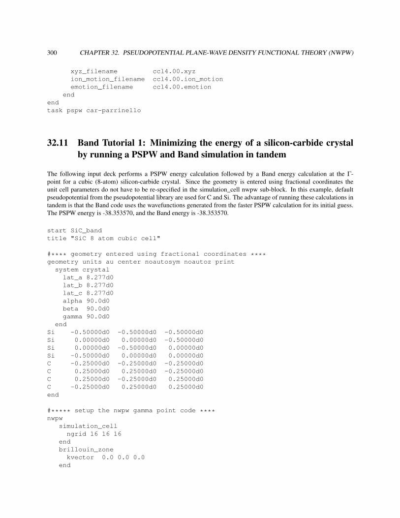
300 CHAPTER 32. PSEUDOPOTENTIAL PLANE-WAVE DENSITY FUNCTIONAL THEORY (NWPW)
xyz_filename ccl4.00.xyzion_motion_filename ccl4.00.ion_motionemotion_filename ccl4.00.emotion
endendtask pspw car-parrinello
32.11 Band Tutorial 1: Minimizing the energy of a silicon-carbide crystalby running a PSPW and Band simulation in tandem
The following input deck performs a PSPW energy calculation followed by a Band energy calculation at the Γ-point for a cubic (8-atom) silicon-carbide crystal. Since the geometry is entered using fractional coordinates theunit cell parameters do not have to be re-specified in the simulation_cell nwpw sub-block. In this example, defaultpseudopotential from the pseudopotential library are used for C and Si. The advantage of running these calculations intandem is that the Band code uses the wavefunctions generated from the faster PSPW calculation for its initial guess.The PSPW energy is -38.353570, and the Band energy is -38.353570.
start SiC_bandtitle "SiC 8 atom cubic cell"
#**** geometry entered using fractional coordinates ****geometry units au center noautosym noautoz print
system crystallat_a 8.277d0lat_b 8.277d0lat_c 8.277d0alpha 90.0d0beta 90.0d0gamma 90.0d0
endSi -0.50000d0 -0.50000d0 -0.50000d0Si 0.00000d0 0.00000d0 -0.50000d0Si 0.00000d0 -0.50000d0 0.00000d0Si -0.50000d0 0.00000d0 0.00000d0C -0.25000d0 -0.25000d0 -0.25000d0C 0.25000d0 0.25000d0 -0.25000d0C 0.25000d0 -0.25000d0 0.25000d0C -0.25000d0 0.25000d0 0.25000d0end
#***** setup the nwpw gamma point code ****nwpw
simulation_cellngrid 16 16 16
endbrillouin_zone
kvector 0.0 0.0 0.0end

32.12. BAND TUTORIAL 2: OPTIMIZING A UNIT CELL AND GEOMETRY FOR SILICON-CARBIDE 301
ewald_ncut 8endset nwpw:minimizer 2set nwpw:psi_brillioun_check .false.task pspw energytask band energy
32.12 BAND Tutorial 2: optimizing a unit cell and geometry for Silicon-Carbide
The following example demonstrates how to uses the BAND module to optimize the unit cell and geometry for asilicon-carbide crystal.
title "SiC 8 atom cubic cell - geometry and unit cell optimization"
start SiC
#**** Enter the geometry using fractional coordinates ****geometry units au center noautosym noautoz print
system crystallat_a 8.277d0lat_b 8.277d0lat_c 8.277d0alpha 90.0d0beta 90.0d0gamma 90.0d0
endSi -0.50000d0 -0.50000d0 -0.50000d0Si 0.00000d0 0.00000d0 -0.50000d0Si 0.00000d0 -0.50000d0 0.00000d0Si -0.50000d0 0.00000d0 0.00000d0C -0.25000d0 -0.25000d0 -0.25000d0C 0.25000d0 0.25000d0 -0.25000d0C 0.25000d0 -0.25000d0 0.25000d0C -0.25000d0 0.25000d0 0.25000d0end
#***** setup the nwpw gamma point code ****nwpw
simulation_cellngrid 16 16 16
endewald_ncut 8monkhorst-pack 2 2 2lmbfgs
end
driverclear

302 CHAPTER 32. PSEUDOPOTENTIAL PLANE-WAVE DENSITY FUNCTIONAL THEORY (NWPW)
maxiter 40endset includestress .true. # this option tells driver to optimize the unit cell#set nwpw:stress_numerical .true. #option to use numerical stresses
task band optimize
32.13 BAND Tutorial 3: optimizing a unit cell and geometry for Aluminumwith fractional occupation
The following example demonstrates how to uses the BAND module to optimize the unit cell and geometry for aAluminum.
title "Aluminum optimization with fractional occupation"
start aluminumfrac
memory 900 mb
geometry noautozsystem crystal
lat_a 3.0lat_b 3.0lat_c 3.0alpha 90.0beta 90.0gamma 90.0
endAl 0.0 0.0 0.0Al 0.0 0.5 0.5Al 0.5 0.5 0.0Al 0.5 0.0 0.5endset nwpw:cif_filename aluminum
nwpwscf andersonmult 1smear temperature 3500.0 fermicutoff 15.0monkhorst-pack 3 3 3ewald_ncut 8mapping 2
endset nwpw:lcao_skip .true.
set includestress .true.#set nwpw:stress_numerical .true.

32.14. PAW TUTORIAL 303
driverclear
endtask band optimize ignore
32.14 PAW Tutorial
The following input deck performs for a water molecule a PSPW energy calculation followed by a PAW energycalculation and a PAW geometry optimization calculation. The default unit cell parameters are used (SC=20.0, ngrid32 32 32). In this simulation, the first PAW run optimizes the wavefunction and the second PAW run optimizes thewavefunction and geometry in tandem.
title "paw steepest descent test"
start paw_test
charge 0
geometry units au nocenter noautoz noautosymO 0.00000 0.00000 0.01390H -1.49490 0.00000 -1.18710H 1.49490 0.00000 -1.18710end
nwpwtime_step 15.8ewald_rcut 1.50tolerances 1.0d-8 1.0d-8
endset nwpw:lcao_iterations 1set nwpw:minimizer 2task pspw energy
task paw energy
nwpwtime_step 5.8geometry_optimizeewald_rcut 1.50tolerances 1.0d-7 1.0d-7 1.0d-4
endtask paw steepest_descent
task paw optimize

304 CHAPTER 32. PSEUDOPOTENTIAL PLANE-WAVE DENSITY FUNCTIONAL THEORY (NWPW)
32.15 PAW Tutorial 2: optimizing a unit cell and geometry for Silicon-Carbide
The following example demonstrates how to uses the PAW module to optimize the unit cell and geometry for a silicon-carbide crystal.
title "SiC 8 atom cubic cell - geometry and unit cell optimization"
start SiC
#**** Enter the geometry using fractional coordinates ****geometry units au center noautosym noautoz print
system crystallat_a 8.277d0lat_b 8.277d0lat_c 8.277d0alpha 90.0d0beta 90.0d0gamma 90.0d0
endSi -0.50000d0 -0.50000d0 -0.50000d0Si 0.00000d0 0.00000d0 -0.50000d0Si 0.00000d0 -0.50000d0 0.00000d0Si -0.50000d0 0.00000d0 0.00000d0C -0.25000d0 -0.25000d0 -0.25000d0C 0.25000d0 0.25000d0 -0.25000d0C 0.25000d0 -0.25000d0 0.25000d0C -0.25000d0 0.25000d0 0.25000d0end
#***** setup the nwpw gamma point code ****nwpw
simulation_cellngrid 16 16 16
endewald_ncut 8
endset nwpw:minimizer 2set nwpw:psi_nolattice .true. # turns of unit cell checking for wavefunctions
driverclearmaxiter 40
endset includestress .true. # this option tells driver to optimize the unit cellset nwpw:stress_numerical .true. #currently only numerical stresses implemented in paw
task paw optimize

32.16. PAW TUTORIAL 2: RUNNING A CAR-PARRINELLO SIMULATION 305
32.16 PAW Tutorial 2: Running a Car-Parrinello Simulation
In this section we show how use the PAW module to perform a Car-Parrinello molecular dynamic simulation for aC2 molecule at the LDA level. Before running a PAW Car-Parrinello simulation the system should be on the Born-Oppenheimer surface, i.e. the one-electron orbitals should be minimized with respect to the total energy (i.e. taskpspw energy). The input needed is basically the same as for optimizing the geometry of a C2 molecule at the LDAlevel, except that and additional Car-Parrinello sub-block is added.
In the following example we show the input needed to run a Car-Parrinello simulation for a C2 molecule at the LDAlevel. In this example, default pseudopotentials from the pseudopotential library are used for C, the boundary conditionis free-space, the exchange correlation functional is LDA, The boundary condition is free-space, and the simulationcell cell is aperiodic and cubic with a side length of 10.0 Angstroms and has 40 grid points in each direction (cutoffenergy is 44 Ry). The time step and fake mass for the Car-Parrinello run are specified to be 5.0 au and 600.0 au,respectively.
start c2_paw_lda_mdtitle "C2 restricted singlet dimer, LDA/44Ry - constant energy Car-Parrinello simulation"
geometryC -0.62 0.0 0.0C 0.62 0.0 0.0end
pspwsimulation_cell units angstroms
boundary_conditions aperiodiclattice
lat_a 10.00d0lat_b 10.00d0lat_c 10.00d0
endngrid 40 40 40
endCar-Parrinello
fake_mass 600.0time_step 5.0loop 10 10
endendset nwpw:minimizer 2task paw energytask paw Car-Parrinello
32.17 NWPW Capabilities and Limitations
• Hybrid Functionals (e.g. PBE0, LDA-SIC) only work in PSPW.
• Car-Parrinello QM/MM simulation only work with PSPW.

306 CHAPTER 32. PSEUDOPOTENTIAL PLANE-WAVE DENSITY FUNCTIONAL THEORY (NWPW)
• Fractional occupations only work for BAND simulations.
32.18 Questions and Difficulties
Questions and encountered problems should be reported to [email protected] or to Eric J. Bylaska, [email protected]

Chapter 33
Electrostatic potentials
The NWChem Electrostatic Potential (ESP) module derives partial atomic charges that fit the quantum mechanicalelectrostatic potential on selected grid points.
The ESP module is specified by the NWChem task directive
task esp
The input for the module is taken from the ESP input block
ESP...
END
33.1 Grid specification
The grid points for which the quantum mechanical electrostatic potential is evaluated and used in the fitting procedureof the partial atomic charges all lie outside the van der Waals radius of the atoms and within a cutoff distance from theatomic centers. The following input parameters determine the selection of grid points.
• If a grid file is found, the grid will be read from that file. If no grid file is found, or the keyword
recalculate
is given, the grid and the electrostatic potential is recalculated.
• The extent of the grid is determined by
range <real rcut>
where rcut is the maximum distance in nm between a grid point and any of the atomic centers. When omitted,a default value for rcut of 0.3 nm is used.
• The grid spacing is specified by
spacing <real spac>
307

308 CHAPTER 33. ELECTROSTATIC POTENTIALS
where spac is the grid spacing in nm for the regularly spaced grid points. If not specified, a default spacing of0.05 nm is used.
• The van der Waals radius of an element can be specified by
radius <integer iatnum> <real atrad>
where iatnum is the atomic number for which a van der Waals radius of atrad in nm will be used in the gridpoint determination. Default values will be used for atoms not specified.
• The probe radius in nm determining the envelope around the molecule is specified by
probe <real probe default 0.07>
• The distance between atomic center and probe center can be multiplied by a constant factor specified by
factor <real factor default 1.0>
All grid points are discarded that lie within a distance factor*(radius(i)+probe) from any atom i.
• Schwarz screening is applied using
screen [<real scrtol default 1.0D-5>]
33.2 Constraints
Additional constraints to the partial atomic charges can be imposed during the fitting procedure. Since point groupsymmetry is ignored during the fitting, contrains must be applied to maintain a symmetric charge.
• The net charge of a subset of atoms can be constrained using
constrain <real charge> {<integer iatom>}
where charge is the net charge of the set of atoms {iatom}. A negative atom number iatom can be used tospecify that the partial charge of that atom is substracted in the sum for the set.
• The net charge of a sequence of atoms can be constrained using
constrain <real charge> <integer iatom> through <integer jatom>
where charge is the net charge of the set of atoms {[iatom:jatom]}.
• A group of atoms can be constrained to have the same charge with
constrain equal {<integer iatom>}
• The individual charge of a group of atoms can be constrained to be equal to those of a second group of atomswith
constrain group <integer iatom> <integer jatom> to <integer katom> <integer latom>

33.3. RESTRAINTS 309
resulting in the same charge for atoms iatom and katom, for atoms iatom+1 and katom+1, ... for atomsjatom and latom.
• A special constraint
constrain xhn <integer iatom> {<integer jatom>}
can be used to constrain the set {iatom,{jatom}} to zero charge, and constrain all atoms in {jatom} tohave the same charge. This can be used, for example, to restrain a methyl group to zero charge, and have allhydrogen carrying identical charges.
33.3 Restraints
Restraints can be applied to each partial charge using the RESP charge fitting procedure.
• The directive for charge restraining is
restrain [hfree] (harmonic [<real scale>] | \hyperbolic [<real scale> [<real tight>]] \[maxiter <integer maxit>] [tolerance <real toler>])
where hfree can be specified to exclude hydrogen atoms from the restaining procecure. Variable scale isthe strength of the restraint potential, with a default of 0.005au for the harmonic restraint and a default valueof 0.001au for the hyperbolic restraint. For the hyperbolic restraints the tightness tight can be specified tochange the default value of 0.1e. The iteration count that needs to be carried out for the hyperbolic restraintis determined by the maximum number of allowed iterations maxiter, with a default value of 25, and thetolerance in the convergence of the partial charges toler, with a default of 0.001e.

310 CHAPTER 33. ELECTROSTATIC POTENTIALS

Chapter 34
Prepare
The prepare module is used to set up the necessary files for a molecular dynamics simulation with NWChem. Usersupplied coordinates can be used to generate topology and restart files. The topology file contains all static informationabout a molecular system, such as lists of atoms, bonded interactions and force field parameters. The restart filecontains all dynamic information about a molecular system, such as coordinates, velocities and properties.
Without any input, the prepare module checks the existence of a topology and restart file for the molecular systems.If these files exist, the module returns to the main task level without action. The module will generate these files whenthey do not exist. Without any input to the module, the generated system will be for a non-solvated isolated solutesystem.
To update existing files, including solvation, the module requires input directives read from an input deck,
prepare...
end
The prepare module performs three sub-tasks:
* sequence generationThis sub-task analyzes the supplied coordinates from a PDB-formatted file or from the input geometry, andgenerates a sequence file, containing the description of the system in terms of basic building blocks found asfragment or segment files in the database directories for the force field used. If these files do not exist, theyare generated based on the supplied coordinates. This process constists of generating a fragment file with thelist of atoms with their force field dependent atom types, partial atomic charges calculated from a Hartree Fockcalculation for the fragment, followed by a restrained electrostatic potential fit, and a connectivity list. Fromthe information on this fragment file the lists of all bonded interactions are generated, and the complete lists arewritten to a segment file.
* topology generationBased on the generated or user-supplied sequence file and the force field specific segment database files, thissub-task compiles the lists of atoms, bonded interactions, excluded pairs, and substitutes the force field param-eters. Special commands may be given to specify interaction parameters that will be changing in a free energyevaluation.
* restart generationUsing the user supplied coordinates and the topology file for the chemical system, this sub-task generates a
311

312 CHAPTER 34. PREPARE
restart file for the system with coordinates, velocities and other dynamic information. This step may includesolvation of the chemical system and specifying periodic boundary conditions.
Files involved in the preparation phase exist in the following hierarchy:
* standardsThe standard database files contain the original force field information. These files are to reside in a directorythat is specified in the file $HOME/.nwchemrc. There will be such a directory for each supported force field.These directories contain fragment files (with extension frg), segment files (with extension sgm) and a parameterfile (with the name of the force field and with extension par).
* extensionsThese database files contain generally accepted extensions to the original force field and are to reside in aseparate directory that is specified in the file $HOME/.nwchemrc. There will be such a directory for eachsupported force field. These directories contain fragment files (with extension frg), segment files (with extensionsgm) and a parameter file (with the name of the force field and with extension par).
* contributedThese database files contain contributed definitions, also required for the quality assurance tests and are to residein a separate directory that is specified in the file $HOME/.nwchemrc. There will be such a directory for eachsupported force field. These directories contain fragment files (with extension frg), segment files (with extensionsgm) and a parameter file (with the name of the force field and with extension par).
* user preferencesThese database files contain user preferred extensions to the original force field and are to reside in a separatedirectory that is specified in the file $HOME/.nwchemrc. Separate directories of this type should be defined foreach supported force field. This directory may contain fragment files (with extension frg), segment files (withextension sgm) and a parameter file (with the name of the force field and with extension par).
* temporary filesTemporary database files contain user preferred extensions to the original force field and are to reside in a sepa-rate directory that is specified in the file $HOME/.nwchemrc. There may be such a directory for each supportedforce field. This directory may contain fragment files (with extension frg), segment files (with extension sgm)and a parameter file (with the name of the force field and with extension par).
* current filesDatabase files that contain user preferred extensions to the original force field and are to reside in a separatedirectory that is specified in the file $HOME/.nwchemrc. Typically this will be the current working directory,although it may be defined as a specific directory. This directory may contain fragment files (with extensionfrg), segment files (with extension sgm) and a parameter file (with the name of the force field and with extensionpar). If not specified, files will be taken from the current directory.
Data is taken from the database files searched in the above order. If data is specified more than once, the last foundvalues are used. For example, if some standard segment is redefined in a temporary file, the latter one will be used.This allows the user to redefine standards or extensions without having to modify those database files, which mayreside in a generally available, non-modifyable directory. If a filename is specified rather than a directory, the filenameindicates the parameter file definition. All other files (frg and sgm files) will be take from the specified directory.
The most common problems with the prepare module are
The format of the pdb file does not conform to the pdb standard. In particular, atom names need to correspondwith definitions in the fragment and segment database files, and should adhere to IUPAC recommendations asadopted by the pdb standard. If this problem occurs, the pdb file will need to be corrected.

34.1. DEFAULT DATABASE DIRECTORIES 313
Non-standard segments may contain atoms that could not be atom typed with the existing typing rules in theforce field parameter files. When this happens, additional typing rules can be included in the parameter file, orthe fragment file may be manually typed.
Parameters for atom types or bonded interactions do not exist in the force field. When this happens, additionalparameters may be defined in the parameter files, or the segment file may be edited to include explicit parameters.
The atoms names in the pdb file do not match the names in the already existing frg or sgm file. NWChem willremove the unknown atoms and replace them with the ones it expects, but the geometry will be changed. It isbest to run the prepare module the first time with the print level set to debug, and to look for messages like “Notfound: atom”. Of course, this is to be expected when using PDB files without explicit hydrogen atoms.
34.1 Default database directories
The file $HOME/.nwchemrc may contain the following entries that determine which files are used by the preparemodule.
ffield <string ffname>
This entry specifies the default force field. Database files supplied with NWChem currently support values forffname of amber, referring to AMBER95, and charmm, referring to the academic CHARMM22 force field.
<string ffname>_(1-9) <string ffdir>[\{<string parfile>\}]
Entries of this type specify the directory ffdir in which force field database files can be found. Optionally theparameterfile in this directory may be specified as parfile. The prepare module will only use files in directoriesspecified here. One exception is that files in the current work directory will be used if no directory with current filesis specified. The directories are read in the order 1-9 with duplicate parameters taken from the last occurrence found.Note that multiple parameter files may be specified that will be read in the order in which they are specified.
<string solvnam> <string solvfil>
This entry may be used to identify a pure solvent restart file solvfil by a name solvnam
An example file $HOME/.nwchemrc is:
ffield amberamber_1 /home/svc-nwchem/nwchem-5.1.1/src/data/amber_s/amber_2 /home/svc-nwchem/nwchem-5.1.1/src/data/amber_x/amber.par,glycam.paramber_3 /home/svc-nwchem/nwchem-5.1.1/src/data/amber_q/spce /home/svc-nwchem/nwchem-5.1.1/src/data/solvents/spce.rstthfs /home/svc-nwchem/nwchem-5.1.1/src/data/solvents/thfs.rstclfm /home/svc-nwchem/nwchem-5.1.1/src/data/solvents/clfm.rstmeoh /home/svc-nwchem/nwchem-5.1.1/src/data/solvents/meoh.rstcharmm_1 /home/svc-nwchem/nwchem-5.1.1/src/data/charmm_s/charmm.parcharmm_2 /home/svc-nwchem/nwchem-5.1.1/src/data/charmm_x/

314 CHAPTER 34. PREPARE
34.2 System name and coordinate source
system <string sys_calc>
The system name can be explicitly specified for the prepare module. If not specified, the system name will betaken from a specification in a previous md input block, or derived from the run time database name.
source ( pdb | rtdb )
The source of the coordinates can be explicitly specified to be from a PDB formatted file sys.pdb, or from ageometry object in the run time database. If not specified, a pdb file will be used when it exists in the current directoryor the rtdb geometry otherwise.
model <integer modpdb default 0>
If a PDB formatted source file contains different MODELs, the model keyword can be used to specify whichMODEL will be used to generate the topology and restart file. If not specified, the first MODEL found on the PDBfile will be read.
altloc <character locpdb default ’ ’>
The altloc keyword may be used to specify the use of alternate location coordinates on a PDB file.
chain <character chnpdb default ’ ’>
The chain keyword may be used to specify the chain identifier for coordinates on a PDB file.
histidine ( hid | hie | hip )
specifies the default protonation state of histidine.
sscyx
Keyword sscyx may be used to rename cysteine residues that form sulphur bridges to CYX.
hbuild
Keyword hbuild may be used to add hydrogen atoms to the unknown segments of the structure found on the pdbfile. Placement of hydrogen atoms is based on geometric criteria, and the resulting fragment and segment files shouldbe carefully examined for correctness.
The database directories are used as specified in the file .nwchemrc. Specific definitions for the force field usedmay be changed in the input file using
directory_(1-9) <string ffdir>[<string parfile>]

34.3. SEQUENCE FILE GENERATION 315
34.3 Sequence file generation
If no existing sequence file is present in the current directory, or if the new_seq keyword was specified in the prepareinput deck, a new sequence file is generated from information from the pdb file, and the following input directives.
maxscf <integer maxscf default 20>
Variable maxscf specifies the maximum number of atoms in a segment for which partial atomic charges will bedetermined from an SCF calculation followed by RESP charge fitting. For larger segments a crude partial chargeguestimation will be done.
qscale <real qscale default 1.0>
Variable qscale specifies the factor with which SCF/RESP determined charges will be multiplied.
modify sequence { <integer sgmnum>:<string sgmnam> }
This command specifies that segment sgmnam should be used for segment with number sgmnum. This commandcan be used to specify a particular protonation state. For example, the following command specifies that residue 114is a hystidine protonated at the Nε site and residue 202 is a hystidine protonated at the Nδ site:
modify sequence 114:HIE 202:HID
Links between atoms can be enforced with
link <string atomname> <string atomname>
For example, to link atom SG in segment 20 with atom FE in segment 55, use:
link 20:_SG 55:FE
The format of the sequence file is given in Table 38.9. In addition to the list of segments this file also includeslinks between non-standard segments or other non-standard links. These links are generated based on distances foundbetween atoms on the pdb file. When atoms are involved in such non-standard links that have not been identified inthe fragment of segment files as a non-chain link atom, the prepare module will ignore these links and report them asskipped. If one or more of these links are required, the user has to include them with explicit link directives in thesequence file, making them forced links. Alternatively, these links can be made forced-links by changing link intoLINK in the sequence file.
fraction { <integer imol> }
Directive fraction can be used to separate solute molecules into fractions for which energies will be separatelyreported during molecular dynamics simulations. The listed molecules will be the last molecule in a fraction. Up to10 molecules may be specified in this directive.
counter <integer num> <string ion>

316 CHAPTER 34. PREPARE
Directive counter adds num counter ions of type ion to the sequence file. Up to 10 counter directives mayappear in the input block.
counter <real factor>
This directive scales the counter ion charge by the specified factor in the determination of counter ions positions.
34.4 Topology file generation
new_top [ new_seq ]
Keyword new_top is used to force the generation of a new topology file. An existing topology file for the systemin the current directory will be overwritten. If keyword new_seq is also specified, an existing sequence file will alsobe overwritten with a newly generated file.
amber | charmm
The prepare module generates force field specific fragment, segment and topology files. The force field may beexplicitly specified in the prepare input block by specifying its name. Currently AMBER and CHARMM are thesupported force fields. A default force field may be specified in the file $HOME/.nwchemrc.
standard <string dir_s>[<string par_s>]extensions <string dir_x>[<string par_x>]contributed <string dir_q>[<string par_q>]user <string dir_u>[<string par_u>]temporary <string dir_t>[<string par_t>]current <string dir_c>[<string par_c>]
The user can explicitly specify the directories where force field specific databases can be found. These includeforce field standards, extensions, quality assurance tests, user preferences, temporary , and current database files.Defaults for the directories where database files reside may be specified in the file $HOME/.nwchemrc for each ofthe supported force fields. Fragment, segment and sequence files generated by the prepare module are written in thetemporary directory. When not specified, the current directory will be used. Topology and restart files are alwayscreated in the current directory.
The following directives control the modifications of a topology file. These directives are executed in the orderin which they appear in the prepare input deck. The topology modifying commands are not stored on the run-timedatabase and are, therefor, not persistent.
modify atom <string atomname> [set <integer mset> | initial | final] \( type <string atomtyp> | charge <real atomcharge> | \
polar <real atompolar> | dummy | self | quantum | quantum_high )
These modify commands change the atom type, partial atomic charge, atomic polarizability, specify a dummy,self-interaction and quantum atom, respectively. If mset is specified, the modification will only apply to the spec-ified set, which has to be 1, 2 or 3. If not specified, the modification will be applied to all three sets. The quan-tum region in QM/MM simulations is defined by specifying atoms with the quantum or quantum_high label.

34.4. TOPOLOGY FILE GENERATION 317
For atoms defined quantum_high basis sets labeled X_H will be used. The atomnam should be specified as<integer isgm>:<string name>, where isgm is the segment number, and name is the atom name. A lead-ing blank in an atom name should be substituted with an underscore. The modify commands may be combined. Forexample, the following directive changes for the specified atom the charge and atom type in set 2 and specifies theatom to be a dummy in set 3.
modify atom 12:_C1 set 2 charge 0.12 type CA set 3 dummy
With the following directives modifications can be made for entire segments.
modify segment <integer isgm> \[protonation <integer iprot> | set <integer mset> | initial | final] \( dummy | self | uncharged | quantum | quantum_high )
where protonation specifies a modification of the default protonation state of the segment as specified in thesegment file. This option only applies to Q-HOP simulations.
Modifications to bonded interaction parameters can be made with the following modify commands.
modify ( bond <string atomtyp> <string atomtyp> | \angle <string atomtyp> <string atomtyp> <string atomtyp> | \
torsion <string atomtyp> <string atomtyp> <string atomtyp> \<string atomtyp> [ multiplicity <integer multip> ] | \plane <string atomtyp> <string atomtyp> <string atomtyp> \<string atomtyp> ) [set <integer mset> | initial | final] \<real value> <real forcon>
where atomtyp and mset are defined as above, multip is the torsion ultiplicity for which the modification isto be applied, value is the reference bond, angle, torsion angle of out-of-plane angle value respectively, and forconis the force constant for bond, angle, torsion angle of out-of-plane angle. When multip or mset are not defined themodification will be applied to all multiplicities and sets, respectively, for the identified bonded interaction.
After modifying atoms to quantum atoms the bonded interactions in which only quantum atoms are involved areremoved from the bonded lists using
update lists
Error messages resulting from parameters not being defined for bonded interaction in which only quantum atomsare involved are ignored using
ignore
To specify that a free energy calculation will be carried out using the topology file, the following keyword needsto be specified,
free
To specify that a Q-HOP simulation will be carried out using the topology file, the following keyword needs to bespecified,

318 CHAPTER 34. PREPARE
qhop
To specify that only the first set of parameters should be used, even if multiple sets have been defined in thefragment or segment files, the following keyword needs to be specified,
first
Note that keywords free, qhop and qhop are mutually exclusive.
34.5 Appending to an existing topology file
noe <string atom1> <string atom3> \<real dist1> <real dist2> <real dist3> <real forc1> <real forc2>
This directive specifies a distance restraint potential between atoms atom1 and atom2, with a harmonic functionwith force constant f orc1 between dist1 and dist2, and a harmonic function with force constant f orc2 between dist2and dist3. For distances shorter than dist1 or larger than dist3, a constant force is applied such that force and energyare continuous at dist1 and dist3, respectively. Distances are given in nm, force constants in kJ mol−1 nm−2.
select <integer isel> { <string atoms> }
Directive select specifies a group of atoms used in the definition of potential of mean force potentials.
The selected atoms are specified by the string atoms which takes the form
[{isgm [ - jsgm ] [,]} [:] [{aname[,]}]
For example, all carbon and oxygen atoms in segments 3 and 6 through 12 are selected for group 1 by
3,6-12:_C????,_O????
pmf [all] [bias] zalign <integer isel> <real forcon1> <real forcon2>pmf [combine] [bias] xyplane <integer isel> <real forcon1> <real forcon2>pmf [constraint] [bias] (distance | zdistance) <integer isel> <integer jsel> \
<real dist1> <real dist2> <real forcon1> <real forcon2>pmf [bias] angle <integer isel> <integer jsel> <integer ksel> \
<real angle1> <real angle2> <real forcon1> <real forcon2>pmf [bias] torsion <integer isel> <integer jsel> <integer ksel> <integer lsel> \
<real angle1> <real angle2> <real forcon1> <real forcon2>pmf [bias] basepair <integer isel> <integer jsel> \
<real dist1> <real dist2> <real forcon1> <real forcon2>pmf [bias] (zaxis | zaxis-cog) <integer isel> <integer jsel> <integer ksel> \
<real dist1> <real dist2> <real forcon1> <real forcon2>
Directive pmf specifies a potential of mean force potential in terms of the specified atom selection. Optionzalign specifies the atoms in the selection to be restrained to a line parallel to the z-axis. Option xyplane specifiesthe atoms in the selection to be restrained to a plane perpendicular to the z-axis. Options distance, angle and

34.6. GENERATING A RESTART FILE 319
torsion, are defined in terms of the center of geometry of the specified atom selections. Keyword basepair isused to specify a harmonic potential between residues isel and jsel. Keywords zaxis and zaxis-cog can beused to pull atoms toward the z-axis. Option all may be specified to apply an equivalent pmf to each of the equiv-alent solute molecules in the system. Option combine may be specified to apply the specified pmf to the atoms inall of the equivalent solute molecules. Option constraint may be specified to a distance pmf to treat the distanceas a contraint. Option bias may be specified to indicate that this function should be treated as a biasing potential.Appropriate corrections to free energy results will be evaluated.
34.6 Generating a restart file
new_rst
Keyword new_rst will cause an existing restart file to be overwritten with a new file.
The follwing directives control the manipulation of restart files, and are executed in the order in which they appearin the prepare input deck.
solvent name <string*3 slvnam default ‘‘HOH’’> \model <string slvmdl default ‘‘spce’’>
The solvent keyword can be used to specify the three letter solvent name as expected on the PDB formatted file,and the name of the solvent model for which solvent coordinates will be used.
solvate [ < real rshell default 1.2 > ] \( [ cube [ <real edge> ]] | \[ box [ <real xedge> [ <real xedge> [ <real xedge> ]]]] | \[ sphere <real radius> ] |[ troct <real edge> ])
Solvation can be specified to be in a cubic box with specified edge, rectangular box with specified edges, or ina sphere with specified radius. Solvation in a cube or rectangular box will automatically also set periodic boundaryconditions. Solvation in a sphere will only allow simulations without periodic boundary conditions. The size of thecubic and rectangular boxes will be expanded by a length specified by the expand variable. If no shape is specified,solvation will be done for a cubic box with an edge that leaves rshell nm between any solute atom and a periodic imageof any solute atom after the solute has been centered. An explicit write is not needed to write the restart file. Thesolvate will write out a file sys_calc.rst. If not specified, the dimension of the solvation cell will be as large asto have at least a distance of rshell nm between any solute atom and the edge of the cell. The experimental troctdirective generates a truncated octrahedral box.
touch <real touch default 0.23>
The variable touch specifies the minimum distance between a solvent and solute atom for which a solventmolecule will be accepted for solvation.
envelope <real xpndw default 0.0>
sets the expand vealues to be used in solvate operations.
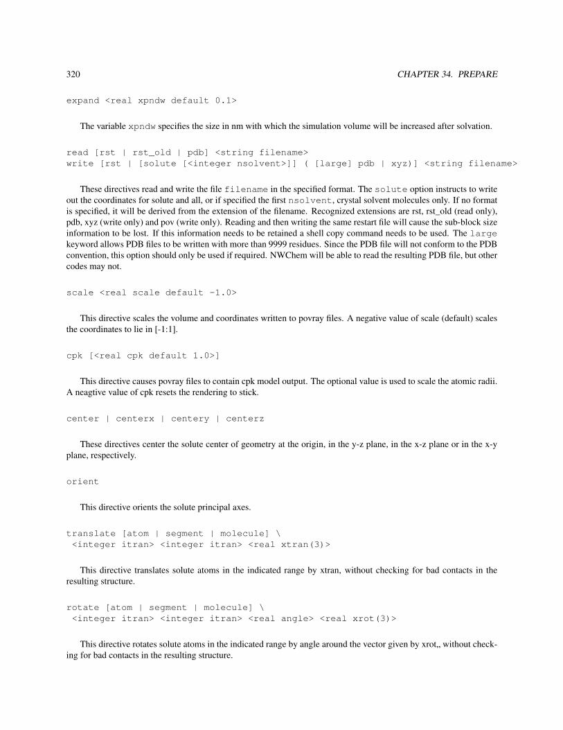
320 CHAPTER 34. PREPARE
expand <real xpndw default 0.1>
The variable xpndw specifies the size in nm with which the simulation volume will be increased after solvation.
read [rst | rst_old | pdb] <string filename>write [rst | [solute [<integer nsolvent>]] ( [large] pdb | xyz)] <string filename>
These directives read and write the file filename in the specified format. The solute option instructs to writeout the coordinates for solute and all, or if specified the first nsolvent, crystal solvent molecules only. If no formatis specified, it will be derived from the extension of the filename. Recognized extensions are rst, rst_old (read only),pdb, xyz (write only) and pov (write only). Reading and then writing the same restart file will cause the sub-block sizeinformation to be lost. If this information needs to be retained a shell copy command needs to be used. The largekeyword allows PDB files to be written with more than 9999 residues. Since the PDB file will not conform to the PDBconvention, this option should only be used if required. NWChem will be able to read the resulting PDB file, but othercodes may not.
scale <real scale default -1.0>
This directive scales the volume and coordinates written to povray files. A negative value of scale (default) scalesthe coordinates to lie in [-1:1].
cpk [<real cpk default 1.0>]
This directive causes povray files to contain cpk model output. The optional value is used to scale the atomic radii.A neagtive value of cpk resets the rendering to stick.
center | centerx | centery | centerz
These directives center the solute center of geometry at the origin, in the y-z plane, in the x-z plane or in the x-yplane, respectively.
orient
This directive orients the solute principal axes.
translate [atom | segment | molecule] \<integer itran> <integer itran> <real xtran(3)>
This directive translates solute atoms in the indicated range by xtran, without checking for bad contacts in theresulting structure.
rotate [atom | segment | molecule] \<integer itran> <integer itran> <real angle> <real xrot(3)>
This directive rotates solute atoms in the indicated range by angle around the vector given by xrot„ without check-ing for bad contacts in the resulting structure.

34.6. GENERATING A RESTART FILE 321
remove solvent [inside | outside] [x <real xmin> <real xmax>] \[y <real ymin> <real ymax>] [z <real zmin> <real zmax>]
This directive removes solvent molecules inside or outside the specified coordinate range.
periodic
This directive enables periodic boundary conditions.
vacuo
This directive disables periodic boundary conditions.
grid <integer mgrid default 24> <real rgrid default 0.2>
This directive specifies the grid size of trial counter-ion positions and minimum distance between an atom in thesystem and a counter-ion.
crop
prints minimum and maximum solute coordinates.
boxsize
specifies to redetermine the box size.
cube
specifies to redetermine the smallest cubic box size.
box <real xsize> <real ysize> <real zsize>
The box directive resets the box size.
align <string atomi> <string atomj> <string atomk>
The align directive orients the system such that atomi and atomj are on the z-axis, and atomk in the x=yplane.
repeat [randomx | randomy | randomz] [chains | molecules | fractions ] \<integer nx> <integer ny> <integer nz> [<real dist>] [<real zdist>]
The repeat directive causes a subsequent write pdb directive to write out multiple copies of the system, withnx copies in the x, ny copies in the y, and nz copies in the z-direction, with a minimum distance of dist betweenany pair of atoms from different copies. If nz is -2, an inverted copy is placed in the z direction, with a separationof zdist nm. If dist is negative, the box dimensions will be used. For systems with solvent, this directive shouldbe used with a negative dist. Optional keywords chains, molecules and fractions specify to write eachrepeating solute unit as a chain, to repeat each solute molecule, or each solute fraction separately. Optional keywordsrandomx, randomy, and randomz can be used to apply random rotations for each repeat unit around a vectorthrough the center of geometry of the solute in the x, y or z direction.

322 CHAPTER 34. PREPARE
skip <integer ix> <integer iy> <integer iz>
The skip directive can be used to skip single repeat unit from the repeat directive. Up to 100 skip directivesmay be specified, and will only apply to the previously specified repeat directive.
(collapsexy | collapsez) [ <integer nmoves>]
specifies to move all solute molecules toward the z-axis or x=y-plane, respectively, to within a distance of touchnm between any pair of atoms from different solute molecules. Parameter nmoves specifies the number of collapsemoves that will be made. Monatomic ions will move with the nearest multi-atom molecule.
collapse_group <integer imol> <integer jmol>
specifies that molecule jmol will move together with molecule imol in collapse operations.
merge <real xtran(3)> <string pdbfile>
specifies to merge the coordinates found on the specified pdb file into the current structure after translation by xtran(3).

Chapter 35
Molecular dynamics
35.1 Introduction
35.1.1 Spacial decomposition
The molecular dynamics module of NWChem uses a distribution of data based on a spacial decomposition of themolecular system, offering an efficient parallel implementation in terms of both memory requirements and communi-cation costs, especially for simulations of large molecular systems.
Inter-processor communication using the global array tools and the design of a data structure allowing distributionbased on spacial decomposition are the key elements in taking advantage of the distribution of memory requirementsand computational work with minimal communication.
In the spacial decomposition approach, the physical simulation volume is divided into rectangular cells, eachof which is assigned to a processor. Depending on the conditions of the calculation and the number of availableprocessors, each processor contains one or more of these spacially grouped cells. The most important aspects of thisdecomposition are the dependence of the cell sizes and communication cost on the number of processors and theshape of the cells, the frequent reassignment of atoms to cells leading to a fluctuating number of atoms per cell, andthe locality of communication which is the main reason for the efficiency of this approach for very large molecularsystems.
To improve efficiency, molecular systems are broken up into separately treated solvent and solute parts. Solventmolecules are assigned to the domains according to their center of geometry and are always owned by a one node. Thisavoids solvent–solvent bonded interactions crossing node boundaries. Solute molecules are broken up into segments,with each segment assigned to a processor based on its center of geometry. This limits the number of solute bondedinteractions that cross node boundaries. The processor to which a particular cell is assigned is responsible for thecalculation of all interactions between atoms within that cell. For the calculation of forces and energies in whichatoms in cells assigned to different processors are involved, data are exchanged between processors. The number ofneighboring cells is determined by the size and shape of the cells and the range of interaction. The data exchange thattakes place every simulation time step represents the main communication requirements. Consequently, one of themain efforts is to design algorithms and data structures to minimize the cost of this communication. However, for verylarge molecular systems, memory requirements also need to be taken into account.
To compromise between these requirements exchange of data is performed in successive point to point communi-cations rather than using the shift algorithm which reduces the number of communication calls for the same amountof communicated data.
323

324 CHAPTER 35. MOLECULAR DYNAMICS
For inhomogeneous systems, the computational load of evaluating atomic interactions will generally differ betweencell pairs. This will lead to load imbalance between processors. Two algorithms have been implemented that allowfor dynamically balancing the workload of each processor. One method is the dynamic resizing of cells such that cellsgradually become smaller on the busiest node, thereby reducing the computational load of that node. Disadvantagesof this method are that the efficiency depends on the solute distribution in the simulation volume and the redistributionof work depends on the number of nodes which could lead to results that depend on the number of nodes used. Thesecond method is based on the dynamic redistribution of intra-node cell-cell interactions. This method represents amore coarse load balancing scheme, but does not have the disadvantages of the cell resizing algorithm. For mostmolecular systems the cell pair redistribution is the more efficient and preferred method.
The description of a molecular system consists of static and dynamic information. The static information doesnot change during a simulation and includes items such as connectivity, excluded and third neighbor lists, equilibriumvalues and force constants for all bonded and non-bonded interactions. The static information is called the topologyof the molecular system, and is kept on a separate topology file. The dynamic information includes coordinates andvelocities for all atoms in the molecular system, and is kept in a so-called restart file.
35.1.2 Topology
The static information about a molecular system that is needed for a molecular simulation is provided to the simulationmodule in a topology file. Items in this file include, among many other things, a list of atoms, their non-bondedparameters for van der Waals and electrostatic interactions, and the complete connectivity in terms of bonds, anglesand dihedrals.
In molecular systems, a distinction is made between solvent and solute, which are treated separately. A solventmolecule is defined only once in the topology file, even though many solvent molecules usually are included in theactual molecular system. In the current implementation only one solvent can be defined. Everything that is not solventin the molecular system is solute. Each solute atom in the system must be explicitly defined in the topology.
Molecules are defined in terms of one or more segments. Typically, repetitive parts of a molecule are each definedas a single segment, such as the amino acid residues in a protein. Segments can be quite complicated to define and are,therefore, collected in a set of database files. The definition of a molecular system in terms of segments is a sequence.
Topology files are created using the prepare module.
35.1.3 Files
File names used have the form $system$_$calc$.$ext$, with exception of the topology file (Section 35.1.2),which is named $system$.top. Anything that refers to the definition of the chemical system can be used for$system$, as long as no periods or underlines are used. The identifier $calc$ can be anything that refers to thetype of calculation to be performed for the system with the topology defined. This file naming convention allowsfor the creation of a single topology file $system$.top that can be used for a number of different calculations,each identified with a different $calc$. For example, if crown.top is the name of the topology file for a crownether, crown_em, crown_md, crown_ti could be used with appropriate extensions for the filenames for energyminimization, molecular dynamics simulation and multi-configuration thermodynamic integration, respectively. Allof these calculations would use the same topology file crown.top.
The extensions <ext> identify the kind of information on a file, and are pre-determined.

35.1. INTRODUCTION 325
dbg debug filefrg fragment filegib free energy data filemri free energy multiple run input filemro free energy multiple run output filenw NWChem input filenwout NWChem output fileout molecular dynamics output filepdb PDB formatted coordinate fileprp property fileqrs quenched restart file, resulting from an energy minimizationrst restart file, used to start or restart a simulationseq sequence file, describing the system in segmentssgm segment file, describing segmentssyn synchronization time filetst test filetim timing analysis filetop topology file, contains the static description of a systemtrj trajectory file
Table 35.1: List of file extensions for nwchem chemical system files.
35.1.4 Databases
Database file supplied with NWChem and used by the prepare module are found in directories with name $ffield$_$level$,where $ffield$ is any of the supported force fields (Section 35.1.5). The source of the data is identified by$level$, and can be
level Descriptions original published datax additional published dataq contributed datau user preferred datat user defined temporary data
The user is can replace these directories or add additional database files by specifying them in the .nwchemrc file.or in the prepare input file.
The extension 1-9 defines the priority of database file.
frg fragmentspar parametersseq sequencessgm segments
Table 35.2: List of database file extensions.
The paths of the different database directories should be defined in a file .nwchemrc in a user’s home directory,and provides the user the option to select which database files are scanned.

326 CHAPTER 35. MOLECULAR DYNAMICS
35.1.5 Force fields
Force fields recognized are
Keyword Force field Statusamber AMBER99 AMBER95,GLYCAM also availablecharmm CHARMM
The units for lengths, angles, and energies are correspondingly nanometers, radians, and kJ/mol.
35.2 Format of fragment files
Fragment files contain the basic information needed to specify all interactions that need to be considered in a molecularsimulation. The format of the fragment files is described in Table 38.1. Normally these files are created by the preparemodule. Manual editing is needed when, for example, the prepare module could not complete atom typing, or whenmodified charges are required.
35.3 Creating segment files
The prepare module is used to generate segment files from corresponding fragment files. A segment file contains allinformation for the calculation of bonded and non-bonded interactions for a given chemical system using a specificforce field.
Which atoms form a fragment is specified in the coordinate file, currently only in PDB format. the restriction isthat bonded interactions may only involve atoms on at most two segments does no longer exist as of NWChem release3.2.1. The segment entries define three sets of parameters for each interaction.
Free energy perturbations can be performed using set 1 for the generation of the ensemble while using sets 2and/or 3 as perturbations. Free energy multiconfiguration thermodynamic integration and multistep thermodynamicperturbation calculations are performed by gradually changing the interactions in the system from parameter set 2 toparameter set 3. These modifications can be edited into the segment files manually, or introduced directly into thetopology file using the modify commands in the input for the prepare module.
The format of a segment is described in Tables 38.2–38.7.
35.4 Creating sequence files
A sequence file describes a molecular system in terms of segments. This file is generated by the prepare module forthe molecular system provided on a PDB-formatted coordinate file. The file format is given in Table 38.9
35.5 Creating topology files
The topology (Section 35.1.2) describes all static information that describes a molecular system. This includes theconnectivity in terms of bond-stretching, angle-bending and torsional interactions, as well as the non-bonded van derWaals and Coulombic interactions.

35.6. CREATING RESTART FILES 327
The topology of a molecular system is generated by the prepare module from the sequence in terms of segments asspecified on the PDB file. For each unique segment specified in this file the segment database directories are searchedfor the segment definition. For segments not found in one of the database directories a segment definition is generatedin the temporary directory if a fragment file was found. If a fragment file could not be found, it is generated by theprepare module base on what is found on the PDB file.
When all segments are found or created, the parameter substitutions are performed, using force field parameterstaken from the parameter databases. After all lists have been generated the topology is written to a local topology file$system$.top.
35.6 Creating restart files
Restart files contain all dynamical information about a molecular system and are created by the prepare moduleif a topology file is available. The prepare module will automatically generate coordinates for hydrogen atoms andmonatomic counter ions not found on the PDB formatted coordinate file, if no fragment or segment files were generatedusing that PDB file.
The prepare module has a number of other optional input command, including solvation.
35.7 Molecular simulations
The type of molecular dynamics simulation is specified by the NWChem task directive.
task md [ energy | optimize | dynamics | thermodynamics ]
where the theory keyword md specifies use of the molecular dynamics module, and the operation keyword is one of
energy for single configuration energy evaluation
optimize for energy minimization
dynamics for molecular dynamics simulations and single step thermodynamic perturbation free energy moleculardynamics simulations
thermodynamics for combined multi-configuration thermodynamic integration and multiple step thermodynamicperturbation free energy molecular dynamics simulations.
35.8 System specification
The chemical system for a calculation is specified in the topology and restart files. These files should be created usingthe utilities nwtop and nwrst before a simulation can be performed. The names of these files are determined from therequired system directive.
system <string systemid>_<string calcid>
where the strings systemid and calcid are user defined names for the chemical system and the type of cal-culation to ber performed, respectively. These names are used to derive the filenames used for the calculation. Thetopoly file used will be systemid.top, while all other files are named systemid_calcid.ext.

328 CHAPTER 35. MOLECULAR DYNAMICS
35.9 Restarting and continuing simulations
finish
specifies that the current job will finish a previous, incomplete simulation, using the input data that have beenrecorded by that previous run in the restart file. Most of the input in the current md input block will be ignored.
resume
specifies that the current job will be an extension of a previous simulation, using most of the input data that havebeen recorded by that previous run in the restart file. Typically the input in the current md input block defines alarger number of steps than the previous job.
35.10 Parameter set
set <integer iset>
specifies the use of parameter set <iset> for the molecular dynamics simulation. The topology file containsthree separate parameters sets that can be used. The default for <iset> is 1.
lambda <integer ilambda> <integer ilambda>
specifies the use of parameter set for the ilambda-th of mlambda steps.
pset <integer isetp1> [<integer isetp2>]
specifies the parameter sets to be used as perturbation potentials in single step thermodynamic perturbation freeenergy evaluations, where <isetp1> specifies the first perturbation parameter set and <isetp2> specifiesthe second perturbation parameter set. Legal values for <isetp1> are 2 and 3. Legal value for <isetp2> is3, in which case <isetp1> can only be 2. If specified, <iset> is automatically set to 1.
pmf [ equilharm <integer npmfc> | scale <real facpmf>]
specifies that any potential of mean force functions defined in the topology files are to be used. If equilharmis specified, the first npmfc dynamics steps will use a harmonic potential in stead of any pmf constraint. Ifscale is specified, all pmf force constants are scaled by a factor facpmf.
distar [draver [<integer ndaver default 1>]][scale <real drsscl>][after <integer nfdrss>]
specifies that any distance restraint functions defined in the topology files are to be used.
qhop [<integer nfhop default 10>][<real rhop default 0.35>][<real thop default 0.02>]
specifies that a Q-HOP simulation is to be carried out with attempted proton hops every n f hop steps, a cutofffor the donor-acceptor pair distance of rhop nm, and a minimum time before back hopping can occur of thopps.
35.11 Energy minimization algorithms
The energy minimization of the system as found in the restart file is performed with the following directives. If bothare specified, steepest descent energy minimization precedes conjugate gradient minimization.

35.12. MULTI-CONFIGURATION THERMODYNAMIC INTEGRATION 329
sd <integer msdit> [init <real dx0sd>] [min <real dxsdmx>] \[max <real dxmsd>]
specifies the variables for steepest descent energy minimizations, where <msdit> is the maximum number ofsteepest descent steps taken, for which the default is 100, <dx0sd> is the initial step size in nm for whichthe default is 0.001, <dxsdmx> is the threshold for the step size in nm for which the default is 0.0001, and<dxmsd> is the maximum allowed step size in nm for which the default is 0.05.
cg <integer mcgit> [init <real dx0cg>] [min <real dxcgmx>] \[cy <integer ncgcy>]
specifies the variables for conjugate gradient energy minimizations, where <mcgit> is the maximum numberof conjugate gradient steps taken, for which the default is 100, <dx0cg> is the initial search interval size innm for which the default is 0.001, <dxcgmx> is the threshold for the step size in nm for which the default is0.0001, and <ncgcy> is the number of conjugate gradient steps after which the gradient history is discardedfor which the default is 10. If conjugate gradient energy minimization is preceded by steepest descent energyminimization, the search interval is set to twice the final step of the steepest descent energy minimization.
35.12 Multi-configuration thermodynamic integration
The following keywords control free energy difference simulations. Multi-configuration thermodynamic integrationsare always combined with multiple step thermodynamic perturbations.
(forward | reverse) [[<integer mrun> of] <integer maxlam>]
specifies the direction and number of integration steps in free energy evaluations, with forward being thedefault direction. <mrun> is the number of ensembles that will be generated in this calculation, and <maxlam>is the total number of ensembles to complete the thermodynamic integration. The default value for <maxlam>is 21. The default value of <mrun> is the value of <maxlam>.
error <real edacq>
specifies the maximum allowed statistical error in each generated ensemble, where <edacq> is the maximumerror allowed in the ensemble average derivative of the Hamiltonian with respect to λ with a default of 5.0kJ mol−1.
drift <real ddacq>
specifies the maximum allowed drift in the free energy result, where <ddacq> is the maximum drift allowedin the ensemble average derivative of the Hamiltonian with respect to λwith a default of 5.0 kJ mol−1ps−1.
factor <real fdacq>
specifies the maximum allowed change in ensemble size where <fdacq> is the minimum size of an ensemblerelative to the previous ensemble in the calculation with a default value of 0.75.
decomp
specifies that a free energy decomposition is to be carried out. Since free energy contributions are path de-pendent, results from a decomposition analysis can no be unambiguously interpreted, and the default is not toperform this decomposition.
sss [delta <real delta>]
specifies that atomic non-bonded interactions describe a dummy atom in either the initial or final state of the ther-modynamic calculation will be calculated using separation-shifted scaling, where <delta> is the separation-shifted scaling factor with a default of 0.075 nm2. This scaling method prevents problems associated withsingularities in the interaction potentials.
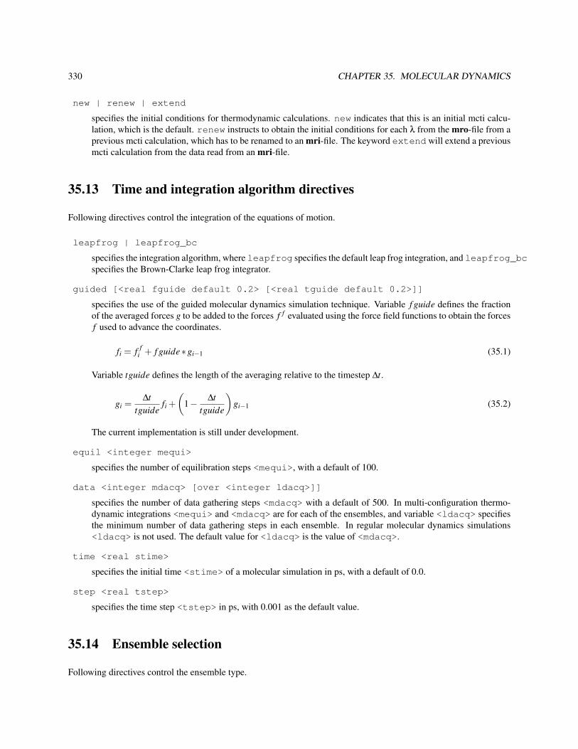
330 CHAPTER 35. MOLECULAR DYNAMICS
new | renew | extend
specifies the initial conditions for thermodynamic calculations. new indicates that this is an initial mcti calcu-lation, which is the default. renew instructs to obtain the initial conditions for each λ from the mro-file from aprevious mcti calculation, which has to be renamed to an mri-file. The keyword extend will extend a previousmcti calculation from the data read from an mri-file.
35.13 Time and integration algorithm directives
Following directives control the integration of the equations of motion.
leapfrog | leapfrog_bc
specifies the integration algorithm, where leapfrog specifies the default leap frog integration, and leapfrog_bcspecifies the Brown-Clarke leap frog integrator.
guided [<real fguide default 0.2> [<real tguide default 0.2>]]
specifies the use of the guided molecular dynamics simulation technique. Variable f guide defines the fractionof the averaged forces g to be added to the forces f f evaluated using the force field functions to obtain the forcesf used to advance the coordinates.
fi = f fi + f guide∗gi−1 (35.1)
Variable tguide defines the length of the averaging relative to the timestep ∆t.
gi =∆t
tguidefi +
(1− ∆t
tguide
)gi−1 (35.2)
The current implementation is still under development.
equil <integer mequi>
specifies the number of equilibration steps <mequi>, with a default of 100.
data <integer mdacq> [over <integer ldacq>]]
specifies the number of data gathering steps <mdacq> with a default of 500. In multi-configuration thermo-dynamic integrations <mequi> and <mdacq> are for each of the ensembles, and variable <ldacq> specifiesthe minimum number of data gathering steps in each ensemble. In regular molecular dynamics simulations<ldacq> is not used. The default value for <ldacq> is the value of <mdacq>.
time <real stime>
specifies the initial time <stime> of a molecular simulation in ps, with a default of 0.0.
step <real tstep>
specifies the time step <tstep> in ps, with 0.001 as the default value.
35.14 Ensemble selection
Following directives control the ensemble type.

35.15. VELOCITY REASSIGNMENTS 331
isotherm [<real tmpext> [<real tmpext2>]] [trelax <real tmprlx> [<real tmsrlx>]] \[anneal [<real tann1>] <real tann2>]
specifies a constant temperature ensemble using Berendsen’s thermostat, where <tmpext> is the externaltemperature with a default of 298.15 K, and <tmprlx> and <tmsrlx> are temperature relaxation times in pswith a default of 0.1. If only <tmprlx> is given the complete system is coupled to the heat bath with relaxationtime <tmprlx>. If both relaxation times are supplied, solvent and solute are independently coupled to the heatbath with relaxation times <tmprlx> and <tmsrlx>, respectively. If keyword anneal is specified, theexternal temperature will change from tmpext to tempext2 between simulation time tann1 and tann2
isobar [<real prsext>] [trelax <real prsrlx> ] \[compress <real compr>] [anisotropic] [xy | z | xy-z]
specifies a constant pressure ensemble using Berendsen’s piston, where <prsext> is the external pressure witha default of 1.025 105 Pa, <prsrlx> is the pressure relaxation time in ps with a default of 0.5, and <compr>is the system compressibility in m2N−1 with a default of 4.53E-10. Optional keywords xy, z and xy-z may beused to specify that pressure scaling is to be applied in the x and y dimension only, the z dimension only, or, in allthree dimensions with identical scaling in the x and y dimension. The last option requires that anisotropicis also specified.
35.15 Velocity reassignments
Velocities can be periodically reassigned to reflect a certain temperature.
vreass <integer nfgaus> <real tgauss>[fraction [<real frgaus default 0.5]][once][(first | initial)] [(last | final)]
specifies that velocities will be reassigned every <nfgaus> molecular dynamics steps, reflecting a temperatureof <tgauss> K. The default is not to reassign velocities, i.e. <nfgaus> is 0. Keyword fraction allowsthe specification of the fraction of the new velocities are random. Keyword once specifies that velocity reas-signment only should be done in the first step. Keywords first or initial and last or final specifythat velocity reassigment should only be applied in the first and last window of multiple run simulations.
35.16 Cutoff radii
Cutoff radii can be specified for short range and long range interactions.
cutoff [short] <real rshort> [long <real rlong>] \[qmmm <real rqmmm>]
specifies the short range cutoff radius <rshort>, and the long range cutoff radius <rlong> in nm. If thelong range cutoff radius is larger than the short range cutoff radius the twin range method will be used, in whichshort range forces and energies are evaluated every molecular dynamics step, and long range forces and energieswith a frequency of <nflong> molecular dynamics steps. Keyword qmmm specifies the radius of the zonearound quantum atoms defining the QM/MM bare charges. The default value for <rshort>, <rlong> and<rqmmm> is 0.9 nm.

332 CHAPTER 35. MOLECULAR DYNAMICS
35.17 Polarization
First order and self consistent electronic polarization models have been implemented.
polar (first | scf [[<integer mpolit>] <real ptol>])
specifies the use of polarization potentials, where the keyword first specifies the first order polarizationmodel, and scf specifies the self consistent polarization field model, iteratively determined with a maximum of<mpolit> iterations to within a tolerance of <ptol> D in the generated induced dipoles. The default is notto use polarization models.
35.18 External electrostatic field
field <real xfield> [freq <real xffreq>] [vector <real xfvect(1:3)>]
specifies an external electrostatic field, where <xfield> is the field strength, <xffreq> is the frequency inMHz and <xfvect> is the external field vector.
35.19 Constraints
Constraints are satisfied using the SHAKE coordinate resetting procedure.
shake [<integer mshitw> [<integer mshits>]] \[<real tlwsha> [<real tlssha>]]
specifies the use of SHAKE constraints, where <mshitw> is the maximum number of solvent SHAKE iter-ations, and <mshits> is the maximum number of solute SHAKE iterations. If only <mshitw> is speci-fied, the value will also be used for <mshits>. The default maximum number of iterations is 100 for both.<tlwsha> is the solvent SHAKE tolerance in nm, and <tlssha> is the solute SHAKE tolerance in nm.If only <tlwsha> is specified, the value given will also be used for <tlssha>. The default tolerance is0.001 nm for both.
noshake (solvent | solute)
disables SHAKE and treats the bonded interaction according to the force field.
35.20 Long range interaction corrections
Long range electrostatic interactions are implemented using the smooth particle mesh Ewald technique, for neutralperiodic cubic systems in the constant volume ensemble, using pair interaction potentials. Particle-mesh Ewald longrange interactions can only be used in molecular dynamics simulations using effective pair potentials, and not in freeenergy simulations, QMD or QM/MM simulations.
pme [grid <integer ng>] [alpha <real ealpha>] \[order <integer morder>] [fft <integer imfft>]\[procs <integer nprocs>] [solvent]
specifies the use of smooth particle-mesh Ewald long range interaction treatment, where ng is the number ofgrid points per dimension, ealpha is the Ewald coefficient in nm−1, with a default that leads to a tolerance

35.21. FIXING COORDINATES 333
of 10−4 at the short range cutoff radius, and morder is order of the Cardinal B-spline interpolation whichmust be an even number and at least 4 (default value). A platform specific 3D fast Fourier transform is used, ifavailable, when imfft is set to 2. nprocs can be used to define a subset of processors to be used to do theFFT calculations. If solvent is specified, the charge grid will be calculated from the solvent charges only.
react [<real dielec default 80.0>]
specifies that a simple reaction field correction is used with a dielectric constant dielec. This is an experi-mental option that has not been well tested.
35.21 Fixing coordinates
Solvent or solute may be fixed using the following keywords.
( fix | free )solvent ( [<integer idfirst> [<integer idlast>]] |
( within | beyond) <real rfix> <string atomname> ) | \solute ( [<integer idfirst> [<integer idlast>]] [ heavy | {<string atomname>}] |
( within | beyond) <real rfix> <string atomname> )[permanent]
For solvent the molecule numbers idfirst and idlastmay be specified to be the first and last molecule towhich the directive applies. If omitted, the directive applies to all molecules. For solute, the segment numbersidfirst and idlastmay be specified to be the first and last segment to which the directive applies. Ifomitted, the directive applies to all segments. In addition, the keyword heavy may be specified to apply to allnon hydrogen atoms in the solute, or a set of atom names may be specified in which a wildcard character ? maybe used. Keyword permanent is used to keep the specification on the restart file for subsequent simulations.
35.22 Special options
import [<integer impfr default 1> [<integer impto default impfr> \[<integer nftri default 1>]]]
specifies the import of frames impfr to impto with frequency nftri from a trajectory file with extensiontri for which energies and forces are to be recalculated. This option only applied to task md energy.
detail
specifies that moments of inertia and radii of gyration will be part of the recorded properties.
profile
specifies that execution time profiling data will be part of the recorded properties.
scale <real scaleq>
specifies that all charges will be scaled by the factro scaleq.
collapse [<real fcoll default 10.0> [ segment | z | xy ]
specifies that additional forces directed to the origin of the simulation cell with strength fcoll will be appliedto all solute molecules. If z or xy is specified, these forces will only apply in the specified dimension(s).

334 CHAPTER 35. MOLECULAR DYNAMICS
include fixed
specifies that energies will be evaluated between fixed atoms. Normally these interactions are excluded from thepairlists.
eqm <real eqm>
specifies the zero point of energy in QMD simulations.
atomlist
specifies that pairlists will be atom based. Normally pairlist are charge group based.
35.23 Autocorrelation function
For the evaluation of the statistical error of multi-configuration thermodynamic integration free energy results a cor-related data analysis is carried out, involving the calculation of the autocorrelation function of the derivative of theHamiltonian with respect to the control variable λ.
auto <integer lacf> [fit <integer nfit>] [weight <real weight>]
controls the calculation of the autocorrelation, where <lacf> is the length of the autocorrelation function, witha default of 1000, <nfit> is the number of functions used in the fit of the autocorrelation function, with adefault of 15, and <weight> is the weight factor for the autocorrelation function, with a default value of 0.0.
35.24 Print options
Keywords that control print to the output file, with extension out. Print directives may be combined to a singledirective.
print [topol [nonbond] [solvent] [solute]] \[step <integer nfoutp> [extra] [energy]] \[stat <integer nfstat>] \[energies [<integer nfener>]] \[forces [<integer nfforce>]] \[matrix] \[expect <integer npxpct>] \[timing] \[pmf [<integer iprpmf>]] \[out6] \[dayout]
Keyword topol specifies printing the topology information, where nonbond refers to the non-bonded inter-action parameters, solvent to the solvent bonded parameters, and solute to the solute bonded parameters.If only topol is specified, all topology information will be printed to the output file.
Keyword step specifies the frequency nfoutp of printing molecular dynamics step information to the outputfile. If the keyword extra is specified additional energetic data are printed for solvent and solute separately.If the keyword energy is specified, information is printed for all bonded solute interactions. The default fornfoutp is 0. For molecular dynamics simulations this frequency is in time steps, and for multi-configurationthermodynamic integration in λ-steps.

35.25. PERIODIC UPDATES 335
Keyword stat specifies the frequency <nfstat> of printing statistical information of properties that arecalculated during the simulation. For molecular dynamics simulation this frequency is in time steps, for multi-configuration thermodynamic integration in λ-steps.
Keyword energies specifies the frequency nfener of printing solute bonded energies the output file forenergy/import calculations. The default for nfener is 0.
Keyword forces specifies the frequency nfforc of printing solute forces the output file for energy/importcalculations. The default for nfforc is 0.
Keyword matrix specifies that a solute distance matrix is to be printed.
Keyword expect is obsolete.
Keyword timing specifies that timing data is printed.
Keyword pmf specifies that pmf data is printed every iprpmf steps. Keyword out6 specifies that output iswritten to standard out in stead of the output file with extension out.
Keyword dayout is obsolete.
35.25 Periodic updates
Following keywords control periodic events during a molecular dynamics or thermodynamic integration simulation.Update directives may be combined to a single directive.
update [pairs <integer nfpair default 1>] \[long <integer nflong default 1>] \[center <integer nfcntr default 0> [zonly | xyonly] \
[fraction <integer idscb(1:5)>] \[motion <integer nfslow default 0>] \[analysis <integer nfanal default 0>] \[rdf <integer nfrdf default 0> \
[range <real rrdf>] [bins <integer ngl>] \
Keyword pairs specifies the frequency <nfpair> in molecular dynamics steps of updating the pair lists. Thedefault for the frequency is 1. In addition, pair lists are also updated after each step in which recording of therestart or trajectory files is performed. Updating the pair lists includes the redistribution of atoms that changeddomain and load balancing, if specified.
Keyword long specifies the frequency <nflong> in molecular dynamics steps of updating the long rangeforces. The default frequency is 1. The distinction of short range and long range forces is only made if the longrange cutoff radius was specified to be larger than the short range cutoff radius. Updating the long range forcesis also done in every molecular dynamics step in which the pair lists are regenerated.
Keywrod center specifies the frequency <nfcntr> in molecular dynamics steps in which the center ofgeometry of the solute(s) is translated to the center of the simulation volume. Optional keyword zonly orxyonly can be used to specify that centering will take place in the z-direction or in the xy-plane only. Thesolute fractions determining the solutes that will be centered are specified by the keyword fraction and thevector <idscb>, with a maximum of 5 entries. This translation is implemented such that it has no effect onany aspect of the simulation. The default is not to center, i.e. nfcntr is 0. The default fraction used to centersolute is 1.
Keyword motion specifies the frequency <nfslow> in molecular dynamics steps of removing the overallrotational and center of mass translational motion.
Keyword analysis specifies the frequency <nfanal> in molecular dynamics steps of invoking the analysismodule. This option is obsolete.

336 CHAPTER 35. MOLECULAR DYNAMICS
Keyword rdf specifies the frequency <nfrdf> in molecular dynamics steps of calculating contributions to theradial distribution functions. The default is 0. The range of the radial distribution functions is given by <rrdf>in nm, with a default of the short range cutoff radius. Note that radial distribution functions are not evaluatedbeyond the short range cutoff radius. The number of bins in each radial distribution function is given by <ngl>,with a default of 1000. This option is no longer supported. If radial distribution function are to be calculated, ardi files needs to be available in which the contributions are specified as follows.
Card Format DescriptionI-1 i Type, 1=solvent-solvent, 2=solvent-solute, 3-solute-soluteI-2 i Number of the rdf for this contributionI-3 i First atom numberI-4 i Second atom number
35.26 Recording
The following keywords control recording data to file. Record directives may be combined to a single directive.
record [rest <integer nfrest> [keep]] \[coord <integer nfcoor default 0>] \[wcoor <integer nfwcoo default 0>] \[scoor <integer nfscoo default 0>] \[veloc <integer nfvelo default 0>] \[wvelo <integer nfwvel default 0>] \[svelo <integer nfsvel default 0>] \[force <integer nfvelo default 0>] \[wforc <integer nfwvel default 0>] \[sforc <integer nfsvel default 0>] \[(prop | prop_average) <integer nfprop default 0>] \[free <integer nffree default 1>] \[sync <integer nfsync default 0>] \[times <integer nftime default 0>] \[acf] [cnv] [fet][binary] [ascii] [ecce] [argos]
Keyword rest specifies the frequency <nfrest> in molecular dynamics steps of rewriting the restart file,with extension rst. For multi-configuration thermodynamic integration simulations the frequency is in steps inλ. The default is not to record. The restart file is used to start or restart simulations. The keyword keep causesall restart files written to be kept on disk, rather than to be overwritten.Keyword coord specifies the frequency <nfcoor> in molecular dynamics steps of writing coordinates to thetrajectory file. This directive redefines previous coord, wcoor and scoor directives. The default is not torecord.Keyword wcoor specifies the frequency <nfcoor> in molecular dynamics steps of writing solvent coordinatesto the trajectory file. This keyword takes precedent over coord. This directive redefines previous coord,wcoor and scoor directives. The default is not to record.Keyword scoor specifies the frequency <nfscoo> in molecular dynamics steps of writing solute coordinatesto the trajectory file. This keyword takes precedent over coord. This directive redefines previous coord,wcoor and scoor directives. The default is not to record.Keyword veloc specifies the frequency <nfvelo> in molecular dynamics steps of writing velocities to thetrajectory file. This directive redefines previous veloc, wvelo and svelo directives. The default is not torecord.

35.27. PROGRAM CONTROL OPTIONS 337
Keyword wvelo specifies the frequency <nfvelo> in molecular dynamics steps of writing solvent velocitiestothe trajectory file. This keyword takes precedent over veloc. This directive redefines previous veloc, wveloand svelo directives. The default is not to record.
Keyword svelo specifies the frequency <nfsvel> in molecular dynamics steps of writing solute velocities tothe trajectory file. This keyword takes precedent over veloc. This directive redefines previous veloc, wveloand svelo directives. The default is not to record.
Keyword force specifies the frequency <nfvelo> in molecular dynamics steps of writing forces to thetrajectory file. This directive redefines previous vforce, wforc and sforc directives. The default is not torecord.
Keyword wforc specifies the frequency <nfvelo> in molecular dynamics steps of writing solvent forcestothe trajectory file. This keyword takes precedent over force. This directive redefines previous vforce,wforc and sforc directives. The default is not to record.
Keyword sforc specifies the frequency <nfsvel> in molecular dynamics steps of writing solute forces to thetrajectory file. This keyword takes precedent over force. This directive redefines previous vforce, wforcand sforc directives. The default is not to record.
Keyword prop specifies the frequency <nfprop> in molecular dynamics steps of writing information to theproperty file, with extension prp. The default is not to record.
Keyword prop_average specifies the frequency <nfprop> in molecular dynamics steps of writing averageinformation to the property file, with extension prp. The default is not to record.
Keyword free specifies the frequency <nffree> in multi-configuration thermodynamic integration steps torecord data to the free energy data file, with extension gib. The default is 1, i.e. to record at every λ. Thisoption is obsolete. All data are required to do the final analysis.
Keyword sync specifies the frequency <nfsync> in molecular dynamics steps of writing information to thesynchronization file, with extension syn. The default is not to record. The information written is the simulationtime, the wall clock time of the previous MD step, the wall clock time of the previous force evaluation, the totalsynchronization time, the largest synchronization time and the node on which the largest synchronization timewas found. The recording of synchronization times is part of the load balancing algorithm. Since load balancingis only performed when pair-lists are updated, the frequency <nfsync> is correlated with the frequency ofpair-list updates <nfpair>. This directive is only needed for analysis of the load balancing performance. Fornormal use this directive is not used.
Keyword times specifies the frequency <nfsync> in molecular dynamics steps of writing information to thetimings file, with extension tim. The default is not to record. The information written is wall clock time usedby each of the processors for the different components in the force evaluation. This directive is only needed foranalysis of the wall clock time distribution. For normal use this directive is not used.
Keywords acf, cnv and fet are obsolete.
Keywords binary, ascii, ecce and argos are obsolete.
35.27 Program control options
load [reset]( none |
size [<real factld>] |sizez [<real factld>] | pairs |
(pairs [<integer ldpair>] size [<real factld>]) )[last][minimum]

338 CHAPTER 35. MOLECULAR DYNAMICS
[average][combination][iotime][experimental]
determines the type of dynamic load balancing performed, where the default is none. Load balancing optionsize is resizing cells on a node, and pairs redistributes the cell-cell interactions over nodes. Keyword resetwill reset the load balancing read from the restart file. The level of cell resizing can be influenced with f actld.The cells on the busiest node are resized with a factor
1− f actld ∗Tsyncnp− tmin
sync
twall
13
(35.3)
where Tsync is the accumulated synchronization time of all nodes, np is the total number of nodes, tminsync is the
synchronization time of the busiest node, and twall is the wall clock time of the molecular dynamics step. Forthe combined load balancing, ldpair is the number of successive pair redistribution load balancing steps inwhich the accumulated synchronization time increases, before a resizing load balancing step will be attempted.Load balancing is only performed in molecular dynamics steps in which the pair-list is updated. The defaultload balancing is equivalent to specifying
load pairs 10 size 0.75
Keyword last specifies that the load balancing is based on the synchronization times of the last step. Thisis the default. Keyword average specifies that the load balancing is based on the average synchronizationtimes since the last load balancing step. Keyword minimum specifies that the load balancing is based on theminimum synchronization times since the last load balancing step. Keywords combination, iotime andexperimental are experimental load balancing options that should not be used in production runs.
(pack | nopack)
specifies if data are communicated in packed or unpacked form. The default is pack.
procs <integer npx> <integer npy> <integer npz>
specifies the distribution of the available processors over the three Cartesian dimensions. The default distribu-tion is chosen such that, <npx>∗<npy>∗<npz>=<np> and <npx> <= <npy> <= <npz>, where <npx>,<npy> and <npz> are the processors in the x, y and z dimension respectively, and <np> is the number ofprocessors allocated for the calculation. Where more than one combination of <npx>, <npy> and <npz>are possible, the combination is chosen with the minimum value of <npx>+<npy>+<npz>. To change thedefault setting the following optional input option is provided.
cells <integer nbx> <integer nby> <integer nbz>
specifies the distribution of cells, where <nbx>, <nby> and <nbz> are the number of cells in x, y and zdirection, respectively. The molecular system is decomposed into cells that form the smallest unit for commu-nication of atomic data between nodes. The size of the cells is per default set to the short-range cutoff radius.If long-range cutoff radii are used the cell size is set to half the long-range cutoff radius if it is larger than theshort-range cutoff. If the number of cells in a dimension is less than the number of processors in that dimension,the number of cells is set to the number of processors.
extra <integer madbox>

35.27. PROGRAM CONTROL OPTIONS 339
sets the number of additional cells for which memory is allocated. In rare events the amount of memory setaside per node is insufficient to hold all atomic coordinates assigned to that node. This leads to execution whichaborts with the message that mwm or msa is too small. Jobs may be restarted with additional space allocated bywhere <madbox> is the number of additional cells that are allocated on each node. The default for <madbox>is 6. In some cases <madbox> can be reduced to 4 if memory usage is a concern. Values of 2 or less willalmost certainly result in memory shortage.
mwm <integer mwmreq>
sets the maximum number of solvent molecules <mwmreq> per node, allowing increased memory to be allo-cated for solvent molecules. This option can be used if execution aborted because mwm was too small.
msa <integer msareq>
sets the maximum number of solute atoms <msareq> per node, allowing increased memory to be allocated forsolute atoms. This option can be used if execution aborted because msa was too small.
mcells <integer mbbreq>
sets the maximum number of cell pairs <mbbreq> per node, allowing increased memory to be allocated for thecell pair lists. This option can be used if execution aborted because mbbl was too small.
boxmin <real rbox>
sets the minimum size of a cell. This directive is obsolete. The use of mcells is preferred.
segmentsize <real rsgm>
sets the maximum size of a segment. This value is used to determine which segments at the boundary of thecutoff radius should be considered in the generation of the pairlists. This value is also determined by the preparemodule and written to the restart file. Use of this directive is not needed for simulations that use the currentprepare module to generate the restart file.
memory <integer memlim>
sets a limit <memlim> in kB on the allocated amount of memory used by the molecular dynamics module. Perdefault all available memory is allocated. Use of this command is required for QM/MM simulations only.
expert
enables the use of certain combinations of features that are considered unsafe. This directive should not be usedfor production runs.
develop <integer idevel>
enables the use of certain development options specified by the integer idevel. This option is for developmentpurposes only, and should not be used for production runs.
control <integer icntrl>
enables the use of certain development options specified by the integer icntrl. This option is for developmentpurposes only, and should not be used for production runs.
numerical
writes out analytical and finite difference forces for test purposes.
server <string servername> <integer serverport>
allows monitoring over a socket connection to the specified port on the named server of basic data as a simulationis running.
For development purposes debug information can be written to the debug file with extension dbg with

340 CHAPTER 35. MOLECULAR DYNAMICS
debug <integer idebug>
where idebug specifies the type of debug information being written.
For testing purposes test information can be written to the test file with extension tst with
test <integer itest>
where itest specifies the number of steps test information is written.
On some platforms prefetching of data can improve the efficiency. This feature can be turned on using
prefetch [<integer nbget>]
where nbget is the number of outstanding communication operations.
Application of periodic boundary conditions for the evaluation of forces can be controlled with
pbc ( atom | residue | molecule )
This option rarely needs to be used.
Autocorrelation functions for error analysis are controlled using
auto [ fit <integer iapprx> | weight <real weight> ]
This option is disabled in the current release.
Membrane system equilibration can be made more efficient using
membrane [ rotations ]
Constraining the center of mass of solute molecules in the xy plane is accomplished using
scmxy [<integer icmopt default 1>]
where icmopt determines if the constraint is mass weighted (2).
Radius of gyration calculations are enabled using
radius_gyration
Calculations of diffusion coefficients is enabled using
diffusion
This option is disabled in the current release.
comlim ( on | off )
is disabled
To limit the size of recoding files, new files are opened every n f new f md steps using
batch <integer nfnewf>

Chapter 36
Analysis
The analysis module is used to analyze molecular trajectories generated by the NWChem molecular dynamics mod-ule, or partial charges generated by the NWChem electrostatic potential fit module. This module should not de run inparallel mode.
Directives for the analysis module are read from an input deck,
analysis...
end
The analysis is performed as post-analysis of trajectory files through using the task directive
task analysis
or
task analyze
36.1 System specification
system <string systemid>_<string calcid>
where the strings systemid and calcid are user defined names for the chemical system and the type of cal-culation to ber performed, respectively. These names are used to derive the filenames used for the calculation. Thetopoly file used will be systemid.top, while all other files are named systemid_calcid.ext.
36.2 Reference coordinates
Most analyses require a set of reference coordinates. These coordinates are read from a NWChem restart file by thedirective,
341

342 CHAPTER 36. ANALYSIS
reference <string filename>
where filename is the name of an existing restart file. This input directive is required.
36.3 File specification
The trajectory file(s) to be analyzed are specified with
file <string filename> [<integer firstfile> <integer lastfile>]
where filename is an existing trj trajectory file. If firstfile and lastfile are specified, the specified filename needs tohave a ? wild card character that will be substituted by the 3-character integer number from firstfile to lastfile, and theanalysis will be performed on the series of files. For example,
file tr_md?.trj 3 6
will instruct the analysis to be performed on files tr_md003.trj, tr_md004.trj, tr_md005.trj and tr_md006.trj.
From the specified files the subset of frames to be analyzed is specified by
frames [<integer firstframe default 1>] <integer lastframe> \[<integer frequency default 1>]
For example, to analyze the first 100 frames from the specified trajectory files, use
frames 100
To analyze every 10-th frame between frames 200 and 400 recorded on the specified trajectory files, use
frames 200 400 10
A time offset can be specified with
time <real timoff>
Solute coordinates of the reference set and ech subsequent frame read from a trajectory file are translated to havethe center of geometry of the specified solute molecule at the center of the simulation box. After this translation allmolecules are folded back into the box according to the periodic boundary conditions. The directive for this operationis
center <integer imol> [<integer jmol default imol>]
Coordinates of each frame read from a trajectory file can be rotated using
rotate ( off | x | y | z ) <real angle units degrees>

36.4. SELECTION 343
If center was defined, rotation takes place after the system has been centered. The rotate directives onlyapply to frames read from the trajectory files, and not to the reference coordinates. Upto 100 rotate directives canbe specified, which will be carried out in the order in which they appear in the input deck. rotate off cancels allpreviously defined rotate directives.
To perform a hydrogen bond analysis:
hbond [distance [[<real rhbmin default 0.0>] <real rhbmin>]] \[angle [<real hbdmin> [ <real hbdmax default pi>]]] \[solvent [<integer numwhb>]]
36.4 Selection
Analyses can be applied to a selection of solute atoms and solvent molecules. The selection is determined by
select ( [ super ] [ { <string atomlist> } ] |solvent <real range> | save <string filename> | read <string filename> )
where {atomlist} is the set of atom names selected from the specified residues. By default all solute atoms areselected. When keyword super is specified the selecion applies to the superimposition option.
The selected atoms are specified by the string atomlist which takes the form
[{isgm [ - jsgm ] [,]} [:] [{aname[,]}]
where isgm and jsgm are the first and last residue numbers, and aname is an atom name. In the atomname a questionmark may be used as a wildcard character.
For example, all protein backbone atoms are selected by
select _N,_CA,_C
To select the backbone atoms in residues 20 to 80 and 90 to 100 only, use
select 20-80,90-100:_N,_CA,_C
This selection is reset to apply to all atoms after each file directive.
Solvent molecules within range nm from any selected solute atom are selected by
select solvent <real range>
After solvent selection, the solute atom selection is reset to being all selected.
The current selection can be saved to, or read from a file using the save and read keywords, respectively.
Some analysis are performed on groups of atoms. These groups of atoms are defined by
define <integer igroup> [<real rsel>] [solvent] { <string atomlist> }
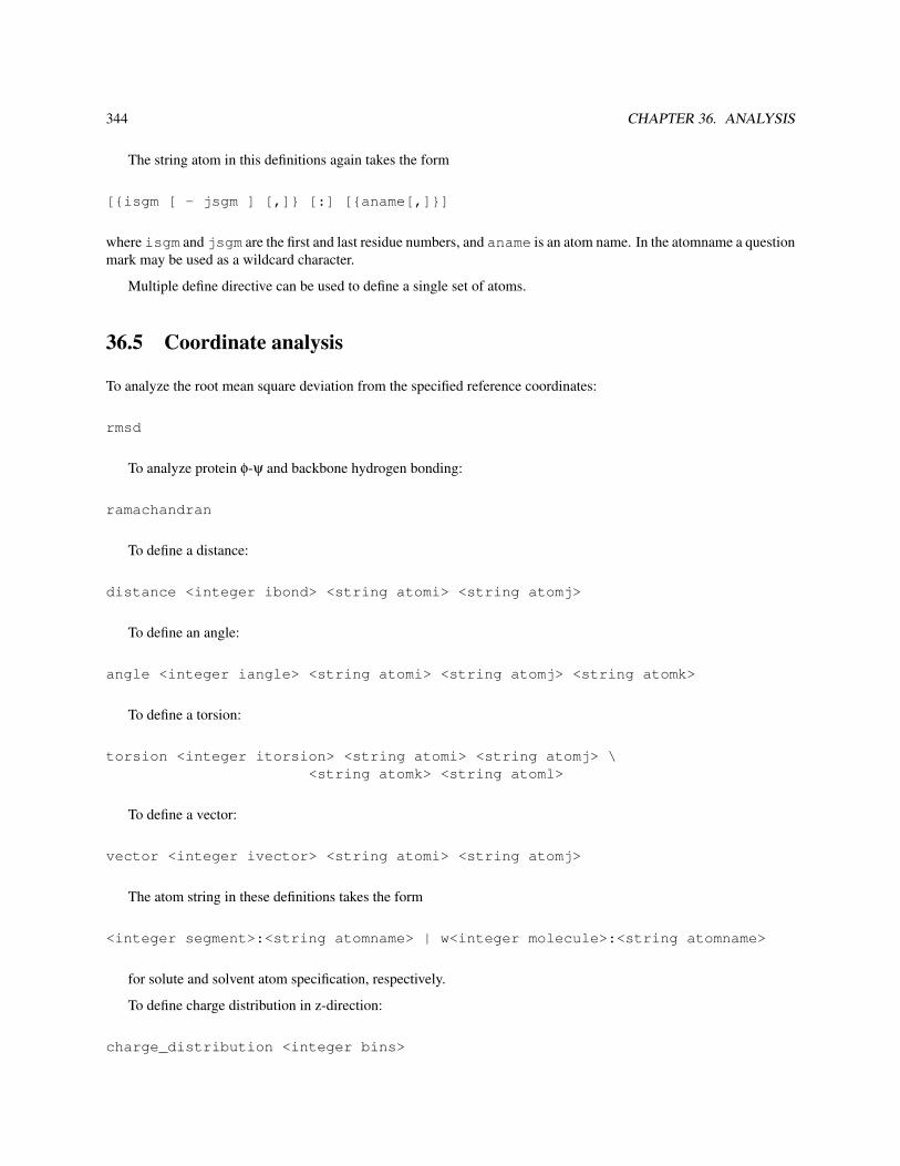
344 CHAPTER 36. ANALYSIS
The string atom in this definitions again takes the form
[{isgm [ - jsgm ] [,]} [:] [{aname[,]}]
where isgm and jsgm are the first and last residue numbers, and aname is an atom name. In the atomname a questionmark may be used as a wildcard character.
Multiple define directive can be used to define a single set of atoms.
36.5 Coordinate analysis
To analyze the root mean square deviation from the specified reference coordinates:
rmsd
To analyze protein φ-ψ and backbone hydrogen bonding:
ramachandran
To define a distance:
distance <integer ibond> <string atomi> <string atomj>
To define an angle:
angle <integer iangle> <string atomi> <string atomj> <string atomk>
To define a torsion:
torsion <integer itorsion> <string atomi> <string atomj> \<string atomk> <string atoml>
To define a vector:
vector <integer ivector> <string atomi> <string atomj>
The atom string in these definitions takes the form
<integer segment>:<string atomname> | w<integer molecule>:<string atomname>
for solute and solvent atom specification, respectively.
To define charge distribution in z-direction:
charge_distribution <integer bins>

36.5. COORDINATE ANALYSIS 345
Analyses on atoms in a predefined group are specified by
group [<integer igroup> [periodic <integer ipbc>] \( local [<real rsel default 0.0>] [<real rval default rsel>]
<string function> )
where igroup specifies the group of atoms defined with a define directive. Keyword periodic can be used tospecify the periodicity, ipbc=1 for periodicity in z, ipbc=2 for periodicity in x and y, and ipbc=3 for periodicityin x, y and z. Currently the only option is local which prints all selected solute atom with a distance between rseland rval from the atoms defined in igroup. The actual analysis is done by the scan deirective. A formatted reportis printed from group analyses using
report <string filename> local
Analyses on pairs of atoms in predefined groups are specified by
groups [<integer igroup> [<integer jgroup>]] [periodic [<integer ipbc default 3>]] \<string function> [<real value1> [<real value2>]] [<string filename>]
where igroup and jgroup are groups of atoms defined with a define directive. Keyword periodic specifiesthat periodic boundary conditions need to be applied in ipbc dimensions. The type of analysis is define by f unction,value1 and value2. If f ilename is specified, the analysis is applied to the reference coordinates and written to the spec-ified file. If no filename is given, the analysis is applied to the specified trajectory and performed as part of the scandirective. Implemented analyses defined by <string function> [<real value1> [<real value2>]]include
distance to calculate the distance between the centers of geometry of the two specified groups of atoms, anddistances to calculate all atomic distances between atoms in the specified groups that lie between value1 andvalue2.
Coordinate histograms are specified by
histogram <integer idef> [<integer length>] zcoordinate <string filename>
where ide f is the atom group definition number, length is the size of the histogram, zcoordinate is the cur-rently only histogram option, and f ilename is the filname to which the histogram is written.
Order parameters are evalated using
order <integer isel> <integer jsel> <string atomi> <string atomj>
This is an experimental feature.
To write the average coordinates of a trajectory
average [super] <string filename>
To perform the coordinate analysis:
scan [ super ] <string filename>
which will create, depending on the specified analysis options files filename.rms and filename.ana. After the scandirective previously defined coordinate analysis options are all reset. Optional keyword super specifies that framesread from the trajectory file(s) are superimposed to the reference structure before the analysis is performed.
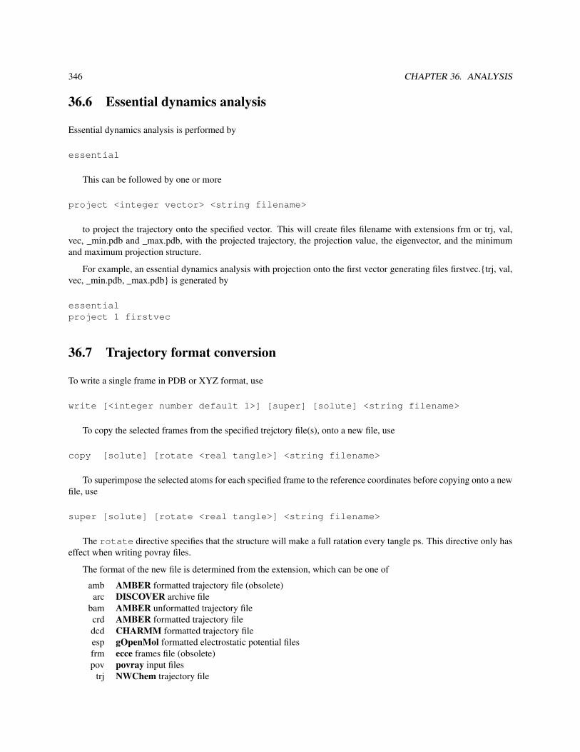
346 CHAPTER 36. ANALYSIS
36.6 Essential dynamics analysis
Essential dynamics analysis is performed by
essential
This can be followed by one or more
project <integer vector> <string filename>
to project the trajectory onto the specified vector. This will create files filename with extensions frm or trj, val,vec, _min.pdb and _max.pdb, with the projected trajectory, the projection value, the eigenvector, and the minimumand maximum projection structure.
For example, an essential dynamics analysis with projection onto the first vector generating files firstvec.{trj, val,vec, _min.pdb, _max.pdb} is generated by
essentialproject 1 firstvec
36.7 Trajectory format conversion
To write a single frame in PDB or XYZ format, use
write [<integer number default 1>] [super] [solute] <string filename>
To copy the selected frames from the specified trejctory file(s), onto a new file, use
copy [solute] [rotate <real tangle>] <string filename>
To superimpose the selected atoms for each specified frame to the reference coordinates before copying onto a newfile, use
super [solute] [rotate <real tangle>] <string filename>
The rotate directive specifies that the structure will make a full ratation every tangle ps. This directive only haseffect when writing povray files.
The format of the new file is determined from the extension, which can be one of
amb AMBER formatted trajectory file (obsolete)arc DISCOVER archive file
bam AMBER unformatted trajectory filecrd AMBER formatted trajectory filedcd CHARMM formatted trajectory fileesp gOpenMol formatted electrostatic potential filesfrm ecce frames file (obsolete)pov povray input files
trj NWChem trajectory file

36.7. TRAJECTORY FORMAT CONVERSION 347
If no extension is specified, a trj formatted file will be written.
A special tag can be added to frm and pov formatted files using
label <integer itag> <string tag> [ <real rval default 1.0> ] \\[ <integer iatag> [ <integer jatag default iatag> ] [ <real rtag default 0.0> ] ][ <string anam> ]
where tag number itag is set to the string tag for all atoms anam within a distance rtag from segments iatagthrough jatag. A question mark can be used in anam as a wild card character.
Atom rendering is specified using
render ( cpk | stick ) [ <real rval default 1.0> ] \\[ <integer iatag> [ <integer jatag default iatag> ] [ <real rtag default 0.0> ] ][ <string anam> ]
for all atoms anam within a distance rtag from segments iatag through jatag, and a scaling factor of rval. Aquestion mark can be used in anam as a wild card character.
Atom color is specified using
color ( <string color> | atom ) \\[ <integer iatag> [ <integer jatag default iatag> ] [ <real rtag default 0.0> ] ][ <string anam> ]
for all atoms anam within a distance rtag from segments iatag through jatag. A question mark can be used inanam as a wild card character.
For example, to display all carbon atoms in segments 34 through 45 in green and rendered cpk in povray files canbe specified with
render cpk 34 45 _C??color green 34 45 _C??
Coordinates written to a pov file can be scaled using
scale <real factor>
A zero or negative scaling factor will scale the coordinates to lie within [-1,1] in all dimensions.
The cpk rendering in povray files can be scaled by
cpk <real factor default 1.0>
The stick rendering in povray files can be scaled by
stick <real factor default 1.0>
The initial sequence number of esp related files is defined by

348 CHAPTER 36. ANALYSIS
index <integer index default 1>
A sequence of trajectory files with unequal lengths can be converted to files with all nclean frames using
clean <integer nclean>
36.8 Electrostatic potentials
A file in plt format of the electrostatic potential resulting from partial charges generated by the ESP module is generatedby the command
esp [ <integer spacing default 10> ] \[ <real rcut default 1.0> ] [periodic [<integer iper default 3>]] \[ <string xfile> [ <string pltfile> ] ]
The input coordinates are taken from the xyzq file that can be generated from a rst by the prepare module. Param-eter spacing specifies the number of gridpoints per nm, rcut specifies extent of the charge grid beyond the molecule.Periodic boundaries will be used if periodic is specified. If iper is set to 2, periodic boundary conditions areapplied in x and y dimensions only. If periodic is specified, a negative value of rcut will extend the grid in theperiodic dimensions by abs(rcut), otherwise this value will be ignored in the periodic dimensions. The resulting pltformatted file pltfile can be viewed with the gOpenMol program. The resulting electrostatic potential grid is in unitsof kJ mol−1e−1. If no files are specified, only the parameters are set. This analysis applies to solute(s) only.
The electrostatic potential at specific point are evaluated using
esp_points [<string filpin> [<string filhol> [<string filpou> [<string filavg>]]]]
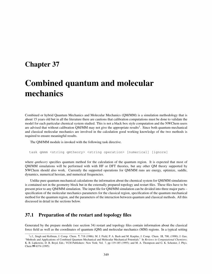
Chapter 37
Combined quantum and molecularmechanics
Combined or hybrid Quantum Mechanics and Molecular Mechanics (QM/MM) is a simulation methodology that isabout 15 years old but in all the literature there are cautions that calibration computations must be done to validate themodel for each particular chemical system studied. This is not a black box style computation and the NWChem usersare advised that without calibration QM/MM may not give the appropriate results1. Since both quantum-mechanicaland classical molecular mechanics are involved in the calculation good working knowledge of the two methods isrequired to ensure meaningful results.
The QM/MM module is invoked with the following task directive.
task qmmm <string qmtheory> <string operation> [numerical] [ignore]
where qmtheory specifies quantum method for the calculation of the quantum region. It is expected that most ofQM/MM simulations will be performed with with HF or DFT theories, but any other QM theory supported byNWChem should also work. Currently the supported operations for QM/MM runs are energy, optimize, saddle,dynamics, numerical hessian, and numerical frequencies.
Unlike pure quantum mechanical calculations the information about the chemical system for QM/MM simulationsis contained not in the geometry block but in the externally prepared topology and restart files. These files have to bepresent prior to any QM/MM simulation. The input file for QM/MM simulation can be divided into three major parts –specification of the molecular mechanics parameters for the classical region, specification of the quantum mechanicalmethod for the quantum region, and the parameters of the interaction between quantum and classical methods. All thisdiscussed in detail in the sections below.
37.1 Preparation of the restart and topology files
Generated by the prepare module (see section 34) restart and topology files contain information about the classicalforce field as well as the coordinates of quantum (QM) and molecular mechanics (MM) regions. In a typical setting
1c.f., Singh and Kollman, J. Comp. Chem. 7, 718 (1986); M. J. Field, P. A. Bash and M. Karplus, J. Comp. Chem. 11, 700, (1990); J. Gao,“Methods and Applications of Combined Quantum Mechanical and Molecular Mechanical Potentials.” In Reviews in Computational Chemistry;K. B. Lipkowitz, D. B. Boyd, Eds.; VCH Publishers: New York; Vol. 7, pp 119-185 (1995); and M. A. Thompson and G. K. Schenter, J. Phys.Chem 99 6374 (1995)
349

350 CHAPTER 37. COMBINED QUANTUM AND MOLECULAR MECHANICS
this "preparation stage" would be run separately from main QM/MM simulation. This will require a properly formattedPDB file for the system. In more complex cases (e.g.non-standard residues or nucleotides) additional fragment andparameter files might have to be provided by the user. The definition of the quantum region in the input for the preparemodule is specified by either modify atom directive (see Section 34):
modify atom <integer isgm>:<string atomname> quantum
or modify segment directive
modify segment <integer isgm> quantum
Here isgm and atomname refer to the residue number and atom name record as given in the PDB file. It isimportant to note that that the leading blanks in atom name record should be indicated with underscores. Per PDBformat quidelines the atom name record starts at column 13. If, for example, the atom name record "OW" startsin the 14th column in PDB file, it will appear as "_OW" in the modify atom directive in the prepare block. In thecurrent implementation only solute atoms can be declared as quantum. If part of the solvent has to be treated quantummechanically then it has to redeclared to be solute. In addition to modify commands the prepare input block shouldalso contain update lists and ignore directives. There are other options that can be used in the input block for theprepare module ( e.g. solvating the structure, etc ), those discussed in more details in Section 34. The successful runof the prepare module will result in generation of topology and restart files. Similar to classical MD, both files arerequired for QM/MM simulations and have to be placed in the same directory as the input file. Here is an exampleinput file that will generate QM/MM restart and topology files for the ethanol molecule
title "Prepare QM/MM calculation of ethanol"start etl
prepare#--name of the pdb file
source etl0.pdb#--generate new topology and sequence file
new_top new_seq#--generate new restart file
new_rst#--define quantum region (note the use of underscore)
modify atom 1:_C1 quantummodify atom 1:2H1 quantummodify atom 1:3H1 quantummodify atom 1:4H1 quantum
#update listsignore
endtask prepare
These are contents of etl0.pdb file used in the above input file.
ATOM 1 O etl 1 1.201 -0.271 -0.000 1.00 0.00 OATOM 2 H etl 1 1.995 0.329 -0.000 1.00 0.00 HATOM 3 C1 etl 1 -1.180 -0.393 0.000 1.00 0.00 C

37.1. PREPARATION OF THE RESTART AND TOPOLOGY FILES 351
ATOM 4 2H1 etl 1 -2.128 0.155 -0.000 1.00 0.00 HATOM 5 3H1 etl 1 -1.130 -1.030 0.887 1.00 0.00 HATOM 6 4H1 etl 1 -1.130 -1.030 -0.887 1.00 0.00 HATOM 7 C2 etl 1 0.006 0.573 0.000 1.00 0.00 CATOM 8 2H2 etl 1 -0.042 1.220 0.890 1.00 0.00 HATOM 9 3H2 etl 1 -0.042 1.220 -0.890 1.00 0.00 HEND
Running the input shown above will produce (among other things) the topology file (etl.top) and the restart file(etl_md.rst). The naming of the topology file follows after the rtdb name specified in the start directive in the input(i.e. "start etl"), while the "_md" suffix in the restart file name is specific to the way prepare module works in thisparticular case. If necessary, this particular naming scheme can be altered using system keyword in the prepare inputblock (for more details see Section 34).
Here is more complicated example where the entire ethanol molecule is declared quantum and solvated in a boxof spce waters:
title "Prepare QM/MM calculation of solvated ethanol"start etlpreparesource etl0.pdbnew_top new_seqnew_rst#center and orient prior to solvationcenterorient#solvation in 1 nm by 2 nm by 3 nm boxsolvate box 1.0 2.0 3.0#the whole ethanol is declared quantum nowmodify segment 1 quantum
update listsignoreendtask prepare
Fixing atoms outside a certain distance from the QM region can also be accomplished using prepare module. Theseconstraints will then be permanently embedded in the resulting restart file, which may be advantageous for cerataintypes of QM/MM simulations. The actual format for the constraint directive to fix whole residues is
fix segments beyond <real radius> <integer residue number>:<string atom name>
or to fix on atom basis
fix atoms beyond <real radius> <integer residue number>:<string atom name>
The following input file illustrated the use of fix segments directive
start etl

352 CHAPTER 37. COMBINED QUANTUM AND MOLECULAR MECHANICS
preparesource etl0.pdbnew_top new_seqnew_rstcenterorient#solvation in 40 A cubic boxsolvate cube 4.0modify segment 1 quantum#fix residues more than 20 A away from ethanol oxygen atomfix segments beyond 2.0 1:_Oupdate listsignoreendtask prepare
37.2 Molecular Mechanics Parameters
The molecular mechanics parameters are given in the form of standard MD input block as used by the MD module (c.f.Section 35). This input block is required for QM/MM simulations. It specifies the restart and topology file that willbe used in the calculation. It also contains information relevant to the calculation of the classical region (e.g. cutoffdistances, constraints, optimization and dynamics parameters, etc) in the system. In this input block one can also setfixed atom constraints on both classical and quantum atoms. Continuing with our example for ethanol molecule hereis a simple input block that may be used for this system.
md# this specifies that etl_md.rst will be used as a restart file# and etl.top will be a topology file
system etl_md# if we ever wanted to fix C1 atom
fix solute 1 _C1end
37.3 Quantum Mechanical Parameters
The parameters defining calculation of the QM region (including basis sets) must be present in the traditional NWCheminput format except for the geometry block. The geometrical information will be constructed automatically usinginformation contained in the restart file
37.4 QM/MM interface parameters
The QM/MM interface parameters define the interaction between classical and quantum regions. The input followsstandard NWChem format:
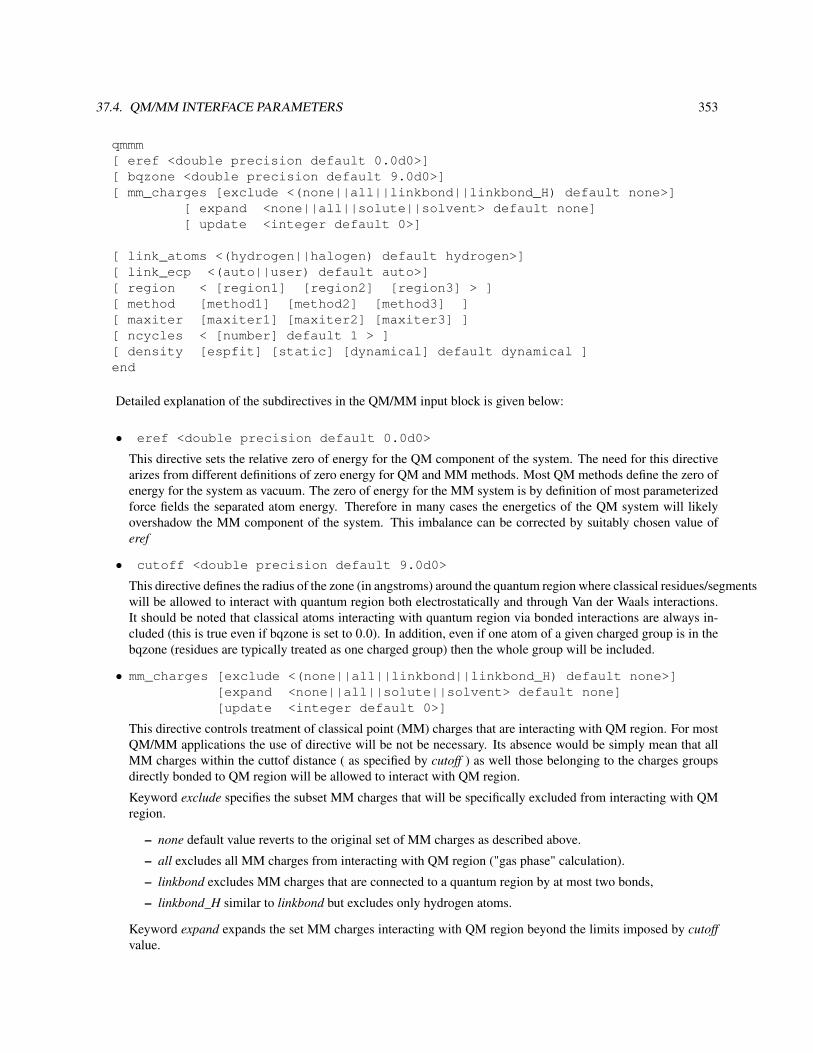
37.4. QM/MM INTERFACE PARAMETERS 353
qmmm[ eref <double precision default 0.0d0>][ bqzone <double precision default 9.0d0>][ mm_charges [exclude <(none||all||linkbond||linkbond_H) default none>]
[ expand <none||all||solute||solvent> default none][ update <integer default 0>]
[ link_atoms <(hydrogen||halogen) default hydrogen>][ link_ecp <(auto||user) default auto>][ region < [region1] [region2] [region3] > ][ method [method1] [method2] [method3] ][ maxiter [maxiter1] [maxiter2] [maxiter3] ][ ncycles < [number] default 1 > ][ density [espfit] [static] [dynamical] default dynamical ]end
Detailed explanation of the subdirectives in the QM/MM input block is given below:
• eref <double precision default 0.0d0>
This directive sets the relative zero of energy for the QM component of the system. The need for this directivearizes from different definitions of zero energy for QM and MM methods. Most QM methods define the zero ofenergy for the system as vacuum. The zero of energy for the MM system is by definition of most parameterizedforce fields the separated atom energy. Therefore in many cases the energetics of the QM system will likelyovershadow the MM component of the system. This imbalance can be corrected by suitably chosen value oferef
• cutoff <double precision default 9.0d0>
This directive defines the radius of the zone (in angstroms) around the quantum region where classical residues/segmentswill be allowed to interact with quantum region both electrostatically and through Van der Waals interactions.It should be noted that classical atoms interacting with quantum region via bonded interactions are always in-cluded (this is true even if bqzone is set to 0.0). In addition, even if one atom of a given charged group is in thebqzone (residues are typically treated as one charged group) then the whole group will be included.
• mm_charges [exclude <(none||all||linkbond||linkbond_H) default none>][expand <none||all||solute||solvent> default none][update <integer default 0>]
This directive controls treatment of classical point (MM) charges that are interacting with QM region. For mostQM/MM applications the use of directive will be not be necessary. Its absence would be simply mean that allMM charges within the cuttof distance ( as specified by cutoff ) as well those belonging to the charges groupsdirectly bonded to QM region will be allowed to interact with QM region.
Keyword exclude specifies the subset MM charges that will be specifically excluded from interacting with QMregion.
– none default value reverts to the original set of MM charges as described above.
– all excludes all MM charges from interacting with QM region ("gas phase" calculation).
– linkbond excludes MM charges that are connected to a quantum region by at most two bonds,
– linkbond_H similar to linkbond but excludes only hydrogen atoms.
Keyword expand expands the set MM charges interacting with QM region beyond the limits imposed by cutoffvalue.
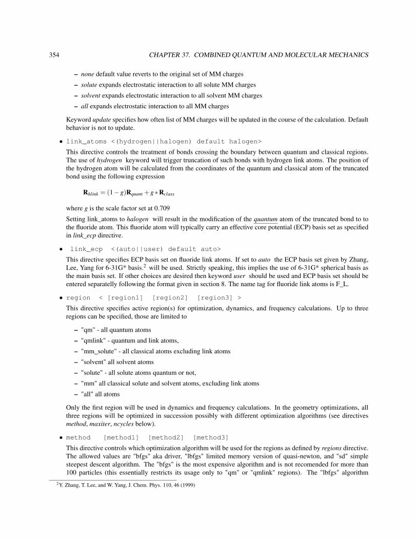
354 CHAPTER 37. COMBINED QUANTUM AND MOLECULAR MECHANICS
– none default value reverts to the original set of MM charges
– solute expands electrostatic interaction to all solute MM charges
– solvent expands electrostatic interaction to all solvent MM charges
– all expands electrostatic interaction to all MM charges
Keyword update specifies how often list of MM charges will be updated in the course of the calculation. Defaultbehavior is not to update.
• link_atoms <(hydrogen||halogen) default halogen>
This directive controls the treatment of bonds crossing the boundary between quantum and classical regions.The use of hydrogen keyword will trigger truncation of such bonds with hydrogen link atoms. The position ofthe hydrogen atom will be calculated from the coordinates of the quantum and classical atom of the truncatedbond using the following expression
Rhlink = (1−g)Rquant +g∗Rclass
where g is the scale factor set at 0.709
Setting link_atoms to halogen will result in the modification of the quantum atom of the truncated bond to tothe fluoride atom. This fluoride atom will typically carry an effective core potential (ECP) basis set as specifiedin link_ecp directive.
• link_ecp <(auto||user) default auto>
This directive specifies ECP basis set on fluoride link atoms. If set to auto the ECP basis set given by Zhang,Lee, Yang for 6-31G* basis.2 will be used. Strictly speaking, this implies the use of 6-31G* spherical basis asthe main basis set. If other choices are desired then keyword user should be used and ECP basis set should beentered separatelly following the format given in section 8. The name tag for fluoride link atoms is F_L.
• region < [region1] [region2] [region3] >
This directive specifies active region(s) for optimization, dynamics, and frequency calculations. Up to threeregions can be specified, those are limited to
– "qm" - all quantum atoms
– "qmlink" - quantum and link atoms,
– "mm_solute" - all classical atoms excluding link atoms
– "solvent" all solvent atoms
– "solute" - all solute atoms quantum or not,
– "mm" all classical solute and solvent atoms, excluding link atoms
– "all" all atoms
Only the first region will be used in dynamics and frequency calculations. In the geometry optimizations, allthree regions will be optimized in succession possibly with different optimization algorithms (see directivesmethod, maxiter, ncycles below).
• method [method1] [method2] [method3]
This directive controls which optimization algorithm will be used for the regions as defined by regions directive.The allowed values are "bfgs" aka driver, "lbfgs" limited memory version of quasi-newton, and "sd" simplesteepest descent algorithm. The "bfgs" is the most expensive algorithm and is not recomended for more than100 particles (this essentially restricts its usage only to "qm" or "qmlink" regions). The "lbfgs" algorithm
2Y. Zhang, T. Lee, and W. Yang, J. Chem. Phys. 110, 46 (1999)

37.4. QM/MM INTERFACE PARAMETERS 355
is recomended for both small and large regions and should be used whenever is possible (in many cases itoutperforms "bfgs"). Finally "sd" the most ineficient and slow way to optimize regions, yet it is the only optionavailable for the optimization of solvent regions. The default is to assign "sd" to optimization involving solventregion (if any), and "lbfgs" to all others.
• maxiter [maxiter1] [maxiter2] [maxiter3]
This directive controls maximum number of iterations for the optimizations of regions as defined by by regionsdirective.
• density [espfit] [static] [dynamical] default dynamical
This directive controls the way electron density of the quantum region is treated when calculating electrostaticinteractions with classical charges. This directive affects QM/MM calculations where both quantum and linkatoms are inactive ( i.e. active region is "mm_solute","solvent", or "mm" ). If set to "espfit" electron density ofthe quantum region will be approximated to by point charges fitted by ESP procedure. This can dramaticallyspeed up both dynamical and optimization tasks that involve purely classical regions. Note that "espfit" optiondoes require movecs file which for example can be obtained by running qmmm energy calculation prior tooptimization. The "static" option will freeze the electron density when quantum and link atoms are inactive. Itis more accurate than "espfit" option but also more expensive. Finally, the default "dynamical" option means thatthe electron density is treated the normal way throught the solution of Schrodinger equation. All calculationsthat involve any geometry changes in quantum or links atoms will automatically use this option.
• ncycles < [number] default 1 >
This directive controls the number of optimization cycles where the defined regions will be optimized in suc-cession. See also etol
• load < esp > [<filename>]
This directive instructs to load external file (located in permanent directory) containing esp charges for QMregion. If filename is not provided it will be constructed from the name of the restart file by replacing ".rst"suffix with ".esp". Note that file containing esp charges is always generated whenever esp charge calculation isperformed,
• convergence < double precision etol default 1.0d-4>
This directive controls convergence of geometry optimization. The optimization is deemed converged if absolutedifference in total energies between consequitive optimization cycles becomes less than etol

356 CHAPTER 37. COMBINED QUANTUM AND MOLECULAR MECHANICS

Chapter 38
File formats
38.1 Format fragment file
38.2 Format segment file
38.3 Format sequence file
38.4 Format trajectory file
38.5 Format free energy file
38.6 Format root mean square deviation file
38.7 Format property file
357
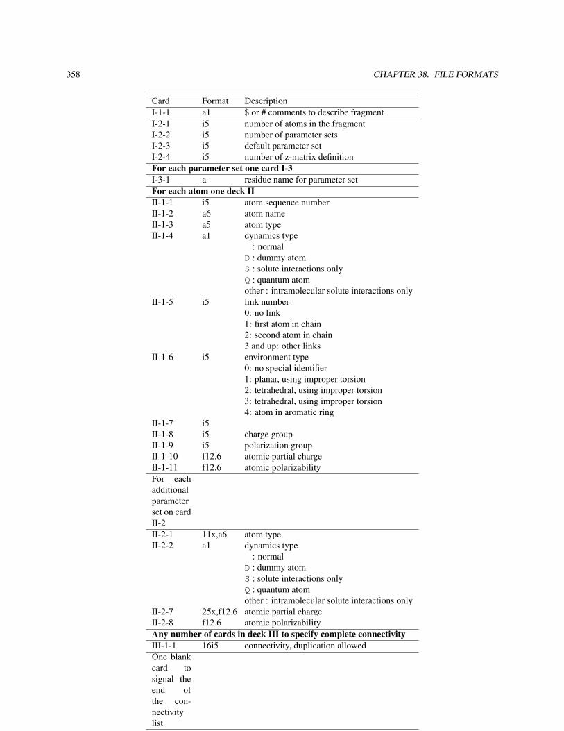
358 CHAPTER 38. FILE FORMATS
Card Format DescriptionI-1-1 a1 $ or # comments to describe fragmentI-2-1 i5 number of atoms in the fragmentI-2-2 i5 number of parameter setsI-2-3 i5 default parameter setI-2-4 i5 number of z-matrix definitionFor each parameter set one card I-3I-3-1 a residue name for parameter setFor each atom one deck IIII-1-1 i5 atom sequence numberII-1-2 a6 atom nameII-1-3 a5 atom typeII-1-4 a1 dynamics type
: normalD : dummy atomS : solute interactions onlyQ : quantum atomother : intramolecular solute interactions only
II-1-5 i5 link number0: no link1: first atom in chain2: second atom in chain3 and up: other links
II-1-6 i5 environment type0: no special identifier1: planar, using improper torsion2: tetrahedral, using improper torsion3: tetrahedral, using improper torsion4: atom in aromatic ring
II-1-7 i5II-1-8 i5 charge groupII-1-9 i5 polarization groupII-1-10 f12.6 atomic partial chargeII-1-11 f12.6 atomic polarizabilityFor eachadditionalparameterset on cardII-2II-2-1 11x,a6 atom typeII-2-2 a1 dynamics type
: normalD : dummy atomS : solute interactions onlyQ : quantum atomother : intramolecular solute interactions only
II-2-7 25x,f12.6 atomic partial chargeII-2-8 f12.6 atomic polarizabilityAny number of cards in deck III to specify complete connectivityIII-1-1 16i5 connectivity, duplication allowedOne blankcard tosignal theend ofthe con-nectivitylistFor eachz-matrixdefinitionone cardIVIV-1-1 i5 atom iIV-1-2 i5 atom jIV-1-3 i5 atom kIV-1-4 i5 atom lIV-1-5 f12.6 bond length i-jIV-1-6 f12.6 angle i-j-kIV-1-7 f12.6 torson i-j-k-l
Table 38.1: The format of fragment files.
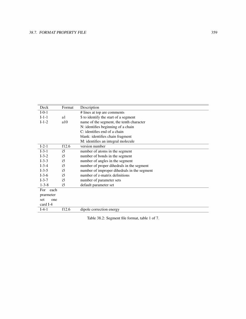
38.7. FORMAT PROPERTY FILE 359
Deck Format DescriptionI-0-1 # lines at top are commentsI-1-1 a1 $ to identify the start of a segmentI-1-2 a10 name of the segment, the tenth character
N: identifies beginning of a chainC: identifies end of a chainblank: identifies chain fragmentM: identifies an integral molecule
I-2-1 f12.6 version numberI-3-1 i5 number of atoms in the segmentI-3-2 i5 number of bonds in the segmentI-3-3 i5 number of angles in the segmentI-3-4 i5 number of proper dihedrals in the segmentI-3-5 i5 number of improper dihedrals in the segmentI-3-6 i5 number of z-matrix definitionsI-3-7 i5 number of parameter sets1-3-8 i5 default parameter setFor eachprarmeterset onecard I-4I-4-1 f12.6 dipole correction energy
Table 38.2: Segment file format, table 1 of 7.

360 CHAPTER 38. FILE FORMATS
Deck Format DescriptionFor each atom one deck IIII-1-1 i5 atom sequence numberII-1-2 a6 atom nameII-1-3 i5 link numberII-1-4 i5 environment type
0: no special identifier1: planar, using improper torsion2: tetrahedral, using improper torsion3: tetrahedral, using improper torsion4: atom in aromatic ring
II-1-5 i5II-1-6 i5 charge groupII-1-7 i5 polarization groupFor eachparameterset onecard II-2II-2-1 5x,a5 atom typeII-2-2 a1 dynamics type
: normalD : dummy atomS : solute interactions onlyQ : quantum atomother : intramolecular solute interactions only
II-2-3 f12.6 atomic partial charge in eII-2-4 f12.6 atomic polarizability/4πεo in nm3
Table 38.3: Segment file format, table 2 of 7.
Deck Format DescriptionFor each bond a deck IIIIII-1-1 i5 bond sequence numberIII-1-2 i5 bond atom iIII-1-3 i5 bond atom jIII-1-4 i5 bond type
0: harmonic1: constrained bond
III-1-5 i5 bond parameter origin0: from database, next card ignored1: from next card
For eachparameterset onecard III-2III-2-1 f12.6 bond length in nmIII-2-2 e12.5 bond force constant in kJ nm2 mol−1
Table 38.4: Segment file format, table 3 of 7.

38.7. FORMAT PROPERTY FILE 361
Deck Format DescriptionFor each angle a deck IVIV-1-1 i5 angle sequence numberIV-1-2 i5 angle atom iIV-1-3 i5 angle atom jIV-1-4 i5 angle atom kIV-1-5 i5 angle type
0: harmonicIV-1-6 i5 angle parameter origin
0: from database, next card ignored1: from next card
For eachparameterset onecard IV-2IV-2-1 f10.6 angle in radiansIV-2-2 e12.5 angle force constant in kJ mol−1
Table 38.5: Segment file format, table 4 of 7.
Deck Format DescriptionFor each proper dihedral a deck VV-1-1 i5 proper dihedral sequence numberV-1-2 i5 proper dihedral atom iV-1-3 i5 proper dihedral atom jV-1-4 i5 proper dihedral atom kV-1-5 i5 proper dihedral atom lV-1-6 i5 proper dihedral type
0: C cos(mφ−δ)V-1-7 i5 proper dihedral parameter origin
0: from database, next card ignored1: from next card
For eachparameterset onecard V-2V-2-1 i3 multiplicityV-2-2 f10.6 proper dihedral in radiansV-2-3 e12.5 proper dihedral force constant in kJ mol−1
Table 38.6: Segment file format, table 5 of 7.
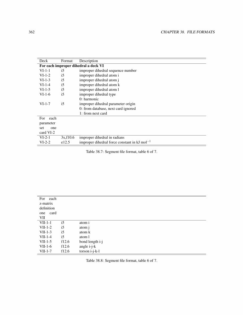
362 CHAPTER 38. FILE FORMATS
Deck Format DescriptionFor each improper dihedral a deck VIVI-1-1 i5 improper dihedral sequence numberVI-1-2 i5 improper dihedral atom iVI-1-3 i5 improper dihedral atom jVI-1-4 i5 improper dihedral atom kVI-1-5 i5 improper dihedral atom lVI-1-6 i5 improper dihedral type
0: harmonicVI-1-7 i5 improper dihedral parameter origin
0: from database, next card ignored1: from next card
For eachparameterset onecard VI-2VI-2-1 3x,f10.6 improper dihedral in radiansVI-2-2 e12.5 improper dihedral force constant in kJ mol−1
Table 38.7: Segment file format, table 6 of 7.
For eachz-matrixdefinitionone cardVIIVII-1-1 i5 atom iVII-1-2 i5 atom jVII-1-3 i5 atom kVII-1-4 i5 atom lVII-1-5 f12.6 bond length i-jVII-1-6 f12.6 angle i-j-kVII-1-7 f12.6 torson i-j-k-l
Table 38.8: Segment file format, table 6 of 7.

38.7. FORMAT PROPERTY FILE 363
Card Format DescriptionI-1-1 a1 $ to identify the start of a sequenceI-1-2 a10 name of the sequenceAny number of cards 1 and 2 in deck II to specify the systemII-1-1 i5 segment numberII-1-2 a10 segment name, last character will be determined from chainII-2-1 a break to identify a break in the molecule chainII-2-1 a molecule to identify the end of a solute moleculeII-2-1 a fraction to identify the end of a solute fractionII-2-1 a5 link to specify a linkII-2-2 i5 segment number of first link atomII-2-3 a4 name of first link atomII-2-4 i5 segment number of second link atomII-2-5 a4 name of second link atomII-2-1 a solvent to identify solvent definition on next cardII-2-1 a stop to identify the end of the sequenceII-2-1 a6 repeat to repeat next ncard cards ncount timesII-2-2 i5 number of cards to repeat (ncards)II-2-3 i5 number of times to repeat cards (ncount)Any number of cards in deck II to specify the system
Table 38.9: Sequence file format.

364 CHAPTER 38. FILE FORMATS
Card Format DescriptionI-1-1 a6 keyword headerI-2-1 i10 number of atoms per solvent moleculeI-2-2 i10 number of solute atomsI-2-3 i10 number of solute bondsI-2-4 i10 number of solvent bondsI-2-5 i10 number of solvent moleculesI-2-6 i10 precision of the coordinates. 0=standard, 1=highFor each atom per solvent molecule one card I-3I-3-1 a5 solvent nameI-3-2 a5 atom nameFor each solute atom one card I-4I-4-1 a5 segment nameI-4-2 a5 atom nameI-4-3 i6 segment numberI-4-4 i10 solute atom counterI-4-5 i5 integer 1For each solvent bond one card I-5I-5-1 i8 atom index i for bond between i and jI-5-2 i8 atom index j for bond between i and jFor each solute bond one card I-6I-6-1 i8 atom index i for bond between i and jI-6-2 i8 atom index j for bond between i and jFor each frame one deck IIII-1-1 a5 keyword frameII-2-1 f12.6 time of frame in psII-2-2 f12.6 temperature of frame in KII-2-3 e12.5 pressure of frame in PaII-2-4 a10 dateII-2-5 a10 timeII-3-1 f12.6 box dimension xII-3-2 12x,f12.6 box dimension yII-3-3 24x,f12.6 box dimension zII-4-1 l1 logical lxw for solvent coordinatesII-4-2 l1 logical lvw for solvent velocitiesII-4-3 l1 logical lfw for solvent forcesII-4-4 l1 logical lpw for solvent induced dipolesII-4-5 l1 logical lxs for solute coordinatesII-4-6 l1 logical lvs for solute velocitiesII-4-7 l1 logical lfs for solute forcesII-4-8 l1 logical lps for solute induced dipolesII-4-5 i10 number of solvent moleculesII-4-6 i10 number of solvent atomsII-4-7 i10 number of solute atoms
Table 38.10: Trajectory file format.

38.7. FORMAT PROPERTY FILE 365
Card Format DescriptionFor each solvent molecule one card II-5 for each atom, if stardard precisionII-5-1 3f8.3 solvent atom coordinates, if lxw or lvwII-5-4 3f8.3 solvent atom velocities, if lvwII-5-7 3f8.1 solvent atom forces, if lfwFor each solute atom one card II-6 for each atom, if stardard precisionII-6-1 3f8.3 solute atom coordinates, if lxs or lvsII-6-4 3f8.3 solute atom velocities, if lvsII-6-7 3f8.1 solute atom forces, if lfsFor each solvent molecule one card II-5 for each atom, if high precisionII-5-1 3e12.6 solvent atom coordinates, if lxw or lvwII-5-4 3e12.6 solvent atom velocities, if lvwII-5-7 3e12.6 solvent atom forces, if lfw (on new card if both lxw and lvw)For each solute atom one card II-6 for each atom, if high precisionII-6-1 3e12.6 solute atom coordinates, if lxs or lvsII-6-4 3e12.6 solute atom velocities, if lvsII-6-7 3e12.6 solute atom forces, if lfs (on new card if both lxs and lvs)
Table 38.11: continued trajectory file format.
Card Format DescriptionFor each step in λ one deck II-1-1 i7 number nderiv of data summed in derivative decomposition array derivI-1-2 i7 length ndata of total derivative array dr fI-1-3 f12.6 current value of λ
I-1-4 f12.6 step size of λ
I-2-1 4e12.12 derivative decomposition array deriv(1 : 24)I-3-1 4e12.12 total derivative array d f r(1 : nda)I-4-1 i10 size of ensemble at current λ
I-4-2 e20.12 average temperature at current λ
I-4-3 e20.12 average exponent reverse perturbation energy at current λ
I-4-4 e20.12 average exponent forward perturbation energy at current λ
Table 38.12: Free energy file format.

366 CHAPTER 38. FILE FORMATS
Card Format DescriptionFor each analyzed time step one card I-1I-1-1 f12.6 time in psI-1-2 f12.6 total rms deviation of the selected atoms before superimpositionI-1-3 f12.6 total rms deviation of the selected atoms after superimpositionII-1-1 a8 keyword analysisFor each solute atom one card II-2II-2-1 a5 segment nameII-2-2 a5 atom nameII-2-3 i6 segment numberII-2-4 i10 atom numberII-2-5 i5 selected if 1II-2-6 f12.6 average atom rms deviation after superimpositionIII-1-1 a8 keyword analysisFor each solute segment one card III-2III-2-1 a5 segment nameIII-2-2 i6 segment numberIII-2-3 f12.6 average segment rms deviation after superimposition
Table 38.13: Root mean square deviation file format.
Card Format DescriptionI-1-1 i7 number nprop of recorded propertiesI-1-2 1x,2a10 date and timeFor each of the nprop properties one card I-2I-2-1 a50 description of recorded propertyFor each recorded step one deck IIII-1-1 4(1pe12.5) value of property
Table 38.14: Property file format.

Chapter 39
Dynamical Nucleation Theory Monte Carlo
1.) Schenter, G. K.; Kathmann, S. M.; Garrett, B. C. J. Chem. Phys. (1999), 110, 7951. 2.)Crosby, L. D.; Kathmann,S. M.; Windus, T. L. J. Comput. Chem. (2008), submitted.
The Dynamical Nucleation Theory Monte Carlo (DNTMC) module utilizes Dynamical Nucleation Theory (DNT)to compute monomer evaporation rate constants at a given temperature. The reactant is a molecular cluster of i rigidmonomers while the product is a molecular cluster with i− 1 monomers plus a free monomer. A Metropolis MonteCarlo (MC) methodology is utilized to sample the configurational space of these i rigid monomers. Both homogenousand heterogenous clusters are supported.
39.1 SubGroups
The DNTMC module supports the use of subgroups in the MC simulations. The number of subgroups is defined inthe input through a set directive:
set subgroup_number <integer number>
,where the number of subgroups requested is the argument. The number of processors that each subgroup has accessto is determined by Total/subgroup_number. A separate MC simulation is performed within each subgroup. To usethis functionality, NWChem must be compiled with the USE_SUBGROUPS environmental variable set.
Each MC simulation starts at a different starting configuration, which is equally spaced along the reaction co-ordinate. The statistical distributions which these MC simulations produce are averaged to form the final statisticaldistribution. Output from these subgroups consists of various files whose names are of the form (*.#num). These filesinclude restart files and other data files. The NWChem runtime database (RTDB) is used as input for these subgroupsand must be globally accessible (set through the Permanent_Dir directive) to all processes.
367

368 CHAPTER 39. DYNAMICAL NUCLEATION THEORY MONTE CARLO
39.2 Input Syntax
The input block has the following form:
DNTMC[nspecies <integer number>][species <list of strings name[nspecies]][nmol <list of integers number[nspecies]>]
[temp <real temperature>][rmin <real rmin>][rmax <real rmax>][nob <integer nob>][mcsteps <integer number>][tdisp <real disp>][rdisp <real rot>][rsim || rconfig][mprnt <integer number>][convergence <real limit>][norestart][dntmc_dir <string directory>]
[print &&|| noprint]
[procrestart <integer number>]END
39.3 Definition of Monomers
Geometry information is required for each unique monomer (species). See the geometry input section 6 for moreinformation. A unique label must be given for each monomer geometry. Additionally, the noautosym and nocenteroptions are suggested for use with the DNTMC module to prevent NWChem from changing the input geometries.Symmetry should also not be used since cluster configurations will seldom exhibit any symmetry; although monomersthemselves may exhibit symmetry.
GEOMETRY [<string name species_1>] noautosym nocenter ......
symmetry c1END
GEOMETRY [<string name species_2>] noautosym nocenter ......
symmetry c1END
...
The molecular cluster is defined by the number of unique monomers (nspecies). The geometry labels for eachunique monomer is given in a space delimited list (species). Also required are the number of each unique monomer

39.4. DNTMC RUNTIME OPTIONS 369
in the molecular cluster given as a space delimited list (nmol). These keywords are required and thus have no defaultvalues.
[nspecies <integer number>][species <list of strings name[nspecies]][nmol <list of integers number[nspecies]>]
An example is shown in section 39.9 for a 10 monomer cluster consisting of a 50/50 mixture of water and ammonia.
39.4 DNTMC runtime options
Several options control the behavior of the DNTMC module. Some required options such as simulation temperature(temp), cluster radius (rmin and rmax), and maximum number of MC steps (mcsteps) are used to control the MCsimulation.
[temp <real temperature>]
This required option gives the simulation temperature in which the MC simulation is run. Temperature is given inkelvin.
[rmin <real rmin>][rmax <real rmax>][nob <integer nob>]
These required options define the minimum and maximum extent of the projected reaction coordinate (The radiusof a sphere centered at the center of mass). Rmin should be large enough to contain the entire molecular cluster ofmonomers and Rmax should be large enough to include any relevant configurational space (such as the position of thereaction bottleneck). These values are given in Angstroms.
The probability distributions obtain along this projected reaction coordinate has a minimum value of Rmin and amaximum value of Rmax. The distributions are created by chopping this range into a number of smaller sized bins.The number of bins (nob) is controlled by the option of the same name.
[mcsteps <integer number>][tdisp <real disp default 0.04>][rdisp <real rot default 0.06>][convergence <real limit default 0.00>]
These options define some characteristics of the MC simulations. The maximum number of MC steps (mcsteps) totake in the course of the calculation run is a required option. Once the MC simulation has performed this number ofsteps the calculation will end. This is a per Markov chain quantity. The maximum translational step size (tdisp) androtational step size (rdisp) are optional inputs with defaults set at 0.04 Angstroms and 0.06 radians, respectively. Theconvergence keyword allows the convergence threshold to be set. The default is 0.00 which effectively turns off thischecking. Once the measure of convergence goes below this threshold the calculation will end.
[rsim || rconfig]

370 CHAPTER 39. DYNAMICAL NUCLEATION THEORY MONTE CARLO
These optional keywords allow the selection of two different MC sampling methods. rsim selects a Metropolis MCmethodology which samples configurations according to a Canonical ensemble. The rconfig keyword selects a MCmethodology which samples configurations according to a derivative of the Canonical ensemble with respect to theprojected reaction coordinate. These keywords are optional with the default method being rconfig.
[mprnt <integer number default 10>][dntmc_dir <string directory default ./>][norestart]
These three options define some of the output and data analysis behavior. mprnt is an option which controls howoften data analysis occurs during the simulation. Currently, every mprnt*nob MC steps data analysis is performed andresults are output to files and/or to the log file. Restart files are also written every mprnt number of MC steps duringthe simulation. The default value is 10. The keyword dntmc_dir allows the definition of an alternate directory to placeDNTMC specific ouputfiles. These files can be very large so be sure enough space is available. This directory shouldbe accessible by every process (although not necessarily globally accessible). The default is to place these files in thedirectory which NWChem is run (./). The keyword norestart turns off the production of restart files. By default restartfiles are produced every mprnt number of MC steps.
39.5 Print Control
The DNTMC module supports the use of PRINT and NOPRINT Keywords. The specific labels which DNTMCrecognizes are included below.
Name Print Level Description“debug” debug Some debug information written in Output file.
“information” none Some information such as energies and geometries.
“mcdata” lowProduction of a set of files (Prefix.MCdata.#num). These files are aconcatenated list of structures, Energies, and Dipole Moments for eachaccepted configuration sampled in the MC run.
“alldata” lowProduction of a set of files (Prefix.Alldata.#num). These files includethe same information as MCdata files. However, they include ALLconfigurations (accepted or rejected).
“mcout” debug – lowProduction of a set of files (Prefix.MCout.#num). These files contain aset of informative and debug information. Also included is the set ofinformation which mirrors the Alldata files.
“fdist” lowProduction of a file (Prefix.fdist) which contains a concatenated list ofdistributions every mprnt*100 MC steps.
“timers” debug
Enables some timers in the code. These timers return performancestatistics in the output file every time data analysis is performed. Twotimers are used. One for the mcloop itself and one for the communica-tion step.

39.6. SELECTED FILE FORMATS 371
39.6 Selected File Formats
Several output files are available in the DNTMC module. This section defines the format for some of these files.
1. *.fdist
This file is a concatenated list of radial distribution functions printed out every mprnt MC steps. Each distributionis normalized (sum equal to one) with respect to the entire (all species) distribution. The error is the RMSdeviation of the average at each point. Each entry is as follows:
[1] # Total Configurations
[2] Species number #
[3](R coordinate in Angstroms) (Probability) (Error)
[Repeats nob times]
[2 and 3 Repeats for each species]
[4] *** separator.
2. *.MCdata.#
This file is a concatenated list of accepted configurations. Each file corresponds to a single Markov chain. Thedipole is set to zero for methods which do not produce a dipole moment with energy calculations. Rsim is eitherthe radial extent of the cluster (r-config) or the simulation radius (r-simulation). Each entry is as follows:
[1] (Atomic label) (X Coord.) (Y Coord.) (Z Coord.)
[1 Repeats for each atom in the cluster configuration, units are in angstroms]
[2] Ucalc = # hartree
[3] Dipole = (X) (Y) (Z) au
[4] Rsim = # Angstrom
[1 through 4 repeats for each accepted configuration]
3. *.MCout.#
This file has the same format and information content as the MCdata file except that additional output is included.This additional output includes summary statistics such as acceptance ratios, average potential energy, andaverage radius. The information included for accepted configurations does not include dipole moment or radius.
4. *.MCall.#
This file has the same format as the MCdata file expect that it includes information for all configurations forwhich an energy is determined. All accepted and rejected configurations are included in this file.
5. *.restart.#
This file contains the restart information for each subgroup. Its format is not very human readable but the basicfields are described in short here.
Random number seed
Potential energy in hartrees
Sum of potential energy
Average potential energy
Sum of the squared potential energy
Squared potential energy

372 CHAPTER 39. DYNAMICAL NUCLEATION THEORY MONTE CARLO
Dipole moment in au (x) (Y) (Z)
Rmin and Rmax
Rsim (Radius corresponds to r-config or r-sim methods)
Array of nspecies length, value indicates the number of each type of monomer which lies at radius Rsimfrom the center of mass [r-simulation sets these to zero]
Sum of Rsim
Average of Rsim
Number of accepted translantional moves
Number of accepted rotational moves
Number of accepted volume moves
Number of attempted moves (volume) (translational) (rotational)
Number of accepted moves (Zero)
Number of accepted moves (Zero)
Number of MC steps completed
[1] (Atom label) (X Coord.) (Y Coord.) (Z Coord.)
[1 repeats for each atom in cluster configurations, units are in angstroms]
[2] Array of nspecies length, number of configurations in bin
[3] Array of nspecies length, normalized number of configurations in each bin
[4] (Value of bin in Angstroms) (Array of nspecies length, normalized probability of bin)
[2 through 4 repeats nob times]
39.7 DNTMC Restart
[procrestart <integer number>]
Flag to indicate restart postprocessing. It is suggested that this postprocessing run is done utilizing only one processor.
In order to restart a DNTMC run, postprocessing is required to put required information into the runtime database(RTDB). During a run restart information is written to files (Prefix.restart.#num) every mprnt MC steps. This infor-mation must be read and deposited into the RTDB before a restart run can be done. The number taken as an argumentis the number of files to read and must also equal the number of subgroups the calculation utilizes. The start directivemust also be set to restart for this to work properly. All input is read as usual. However, values from the restart filestake precedence over input values. Some keywords such as mcsteps are not defined in the restart files. Task directivesare ignored. You must have a RTDB present in your permanent directory.
Once postprocessing is done a standard restart can be done from the RTDB by removing the procrestart keywordand including the restart directive.
39.8 Task Directives
The DNTMC module can be used with any level of theory which can produce energies. Gradients and Hessians arenot required within this methodology. If dipole moments are available, they are also utilized. The task directive forthe DNTMC module is shown below:

39.9. EXAMPLE 373
task <string theory> dntmc
39.9 Example
This example is for a molecular cluster of 10 monomers. A 50/50 mixture of water and ammonia. The energies aredone at the SCF/6-31++G** level of theory.
start# start or restart directive if a restart runMEMORY 1000 mb
PERMANENT_DIR /home/bill# Globally accessible directory which the# rtdb (*.db) file will/does reside.
basis "ao basis" spherical noprint
* library 6-31++G**end# basis set directive for scf energies
scfsingletrhftol2e 1.0e-12vectors input atomicthresh 1.0e-06maxiter 200print none
end# scf directive for scf energies
geometry geom1 units angstroms noautosym nocenter noprintO 0.393676503613369 -1.743794626956820 -0.762291912129271H -0.427227157125777 -1.279138812526320 -0.924898279781319H 1.075463952717060 -1.095883929075060 -0.940073459864222symmetry c1end# geometry of a monomer with title "geom1"
geometry geom2 units angstroms noautosym nocenter noprintN 6.36299e-08 0.00000 -0.670378H 0.916275 0.00000 -0.159874H -0.458137 0.793517 -0.159874H -0.458137 -0.793517 -0.159874symmetry c1end# geometry of another monomer with title "geom2"# other monomers may be included with different titles

374 CHAPTER 39. DYNAMICAL NUCLEATION THEORY MONTE CARLO
set subgroups_number 8# set directive which gives the number of subgroups# each group runs a separate MC simulation
dntmc# DNTMC input block
nspecies 2# The number of unique species (number of titled geometries# above)species geom1 geom2# An array of geometry titles (one for each# nspecies/geometry)nmol 5 5# An array stating the number of each# monomer/nspecies/geometry in simulation.temp 243.0mcsteps 1000000rmin 3.25rmax 12.25mprnt 10tdisp 0.04rdisp 0.06print none fdist mcdata# this print line first sets the print-level to none# then it states that the *.fdist and *.mcdata.(#num)# files are to be writtenrconfigdntmc_dir /home/bill/largefile# An accessible directory which to place the *.fdist,# *.mcdata.(#num), and *.restart.(#num) files.convergence 1.0D+00
end
task scf dntmc# task directive stating that energies are to be done at the scf#level of theory.

Chapter 40
Controlling NWChem with Python
Python (version 1.5.1) programs may be embedded into the NWChem input and used to control the execution ofNWChem. Python is a very powerful and widely used scripting language that provides useful things such as variables,conditional branches and loops, and is also readily extended. Example applications include scanning potential energysurfaces, computing properties in a variety of basis sets, optimizing the energy w.r.t. parameters in the basis set,computing polarizabilities with finite field, and simple molecular dynamics.
Look in the NWChem contrib directory for useful scripts and examples. Visit the Python web-site http://www.python.orgfor a full manual and lots of useful code and resources.
40.1 How to input and run a Python program inside NWChem
A Python program is input into NWChem inside a Python compound directive.
python [print|noprint]...
end
The END directive must be flush against the left margin (see the Troubleshooting section for the reason why).
The program is by default printed to standard output when read, but this may be disabled with the noprint key-word. Python uses indentation to indicate scope (and the initial level of indentation must be zero), whereas NWChemuses optional indentation only to make the input more readable. For example, in Python, the contents of a loop,or conditionally-executed block of code must be indented further than the surrounding code. Also, Python attachesspecial meaning to several symbols also used by NWChem. For these reasons, the input inside a PYTHON compounddirective is read verbatim except that if the first line of the Python program is indented, the same amount of indentationis removed from all subsequent lines. This is so that a program may be indented inside the PYTHON input block forimproved readability of the NWChem input, while satisfying the constraint that when given to Python the first line haszero indentation.
E.g., the following two sets of input specify the same Python program.
pythonprint ’Hello’print ’Goodbye’
375

376 CHAPTER 40. CONTROLLING NWCHEM WITH PYTHON
end
pythonprint ’Hello’print ’Goodbye’end
whereas this program is in error since the indentation of the second line is less than that of the first.
pythonprint ’Hello’
print ’Goodbye’end
The Python program is not executed until the following directive is encountered
task python
which is to maintain consistency with the behavior of NWChem in general. The program is executed by all nodes.This enables the full functionality and speed of NWChem to be accessible from Python, but there are some gotchas
• Print statements and other output will be executed by all nodes so you will get a lot more output than probablydesired unless the output is restricted to just one node (by convention node zero).
• The calls to NWChem functions are all collective (i.e., all nodes must execute them). If these calls are not madecollectively your program may deadlock (i.e., cease to make progress).
• When writing to the database (rtdb_put()) it is the data from node zero that is written.
• NWChem overrides certain default signal handlers so care must be taken when creating processes (see Section40.3.11).
40.2 NWChem extensions
Since we have little experience using Python, the NWChem-Python interface might change in a non-backwardly com-patible fashion as we discover better ways of providing useful functionality. We would appreciate suggestions aboutuseful things that can be added to the NWChem-Python interface. In principle, nearly any Fortran or C routine withinNWChem can be extended to Python, but we are also interested in ideas that will enable users to build completelynew things. For instance, how about being able to define your own energy functions that can be used with the existingoptimizers or dynamics package?
Python has been extended with a module named "nwchem" which is automatically imported and contains the fol-lowing NWChem-specific commands. They all handle NWChem-related errors by raising the exception "NWChemError",which may be handled in the standard Python manner (see Section 40.3.9).
• input_parse(string) — invokes the standard NWChem input parser with the data in string as input.Note that the usual behavior of NWChem will apply — the parser only reads input up to either end of input oruntil a TASK directive is encountered (the task directive is not executed by the parser).
• task_energy(theory)— returns the energy as if computed with the NWChem directive TASK ENERGY <THEORY>.

40.2. NWCHEM EXTENSIONS 377
• task_gradient(theory) — returns a tuple (energy,gradient) as if computed with the NWChemdirective TASK GRADIENT <THEORY>.
• task_optimize(theory) — returns a tuple (energy,gradient) as if computed with the NWChemdirective TASK OPTIMIZE <THEORY>. The energy and gradient will be those at the last point in the opti-mization and consistent with the current geometry in the database.
• task_freq(theory) — returns a tuple directive TASK FREQ <THEORY>. They will be consistent withthe current geometry in the database.
• task_property(theory)— returns the energy as if computed with the NWChem directive TASK PROPERIY <THEORY>.
• task_stress(theory) — returns a tuple (energy,gradient,stress) as if computed with theNWChem directive TASK STRESS <THEORY>. The energy and gradient will be consistent with the currentgeometry in the database.
• task_lstress(theory) — returns a tuple (energy,gradient,lstress). The energy and gradientwill be consistent with the current geometry in the database.
• task_hessian(theory) — performs a hessian calculation as if requested with the NWChem directiveTASK HESSIAN <THEORY>. They will be consistent with the current geometry in the database.
• task_saddle(theory) — returns a tuple (energy,gradient) as if computed with the NWChemdirective TASK SADDLE <THEORY>. The energy and gradient will be those at the last point in the search andconsistent with the current geometry in the database.
• task_coulomb(theory) — returns the couloumb energy. It will be consistent with the current geometryin the database.
• task_coulomb_ref(theory) — returns the couloumb reference energy. It will be consistent with thecurrent geometry in the database.
• ga_nodeid() — returns the GA number of the parallel process.
• ga_groupid() — returns the GA group ID.
• pgroup_create(num) — create num process groups. Must be called by all members of current group.
• pgroup_destroy() — destroy current group. Must be called by all members of current group.
• pgroup_sync() — a barrier that all processes in a goup must get to before they are allowed to continue.
• pgroup_sync_all() — sync all processes regardless of process groups.
• pgroup_global_op() — a global operation within a group. This is like the MPI DGOP/IGOP commands.This input list or numbers or single number must be the same on all nodes. If no operation is included then “+”is assumed.
• pgroup_global_op_all() — a global operation regardless of process groups.
• pgroup_global_op_zero() — a global operation among the zero nodes of the current set of groups. ie.one level up from the lowest level.
• pgroup_broadcast() — a broadcast within a group. This is like the MPI broadcst command. Node zeroof the group always does the talking. All nodes must pass in the same sized object (list of numbers or a singlenumber) and will recieve the same sized object.
• pgroup_broadcast_all() — a broadcast regardless of process groups.

378 CHAPTER 40. CONTROLLING NWCHEM WITH PYTHON
• pgroup_broadcast_zero() — a broadcast among the zero nodes of the current set of groups. ie. onelevel up from the lowest level.
• pgroup_nnodes() — the number of nodes within the current group.
• pgroup_nodeid() — the node ID within the current group.
• pgroup_groupid() — the group ID of the current group.
• pgroup_ngroups() — the number of groups at the current group level.
• rtdb_print(print_values) — prints the contents of the RTDB. If print_values is 0, only the keysare printed, if it is 1 then the values are also printed.
• rtdb_put(name, values) or rtdb_put(name, values, type)— puts the values into the databasewith the given name. In the first form, the type is inferred from the first value, and in the second form the typeis specified using the last argument as one of INT, DBL, LOGICAL, or CHAR.
• rtdb_get(name) — returns the data from the database associated with the given name.
An example below (Section 40.3.10) explains, in lieu of a Python wrapper for the geometry object, how to obtainthe Cartesian molecular coordinates directly from the database.
40.3 Examples
Several examples will provide the best explanation of how the extensions are used, and how Python might prove useful.
40.3.1 Hello world
pythonprint ’Hello world from process ’, ga_nodeid()
end
task python
This input prints the traditional greeting from each parallel process.
40.3.2 Scanning a basis exponent
geometry units auO 0 0 0; H 0 1.430 -1.107; H 0 -1.430 -1.107
end
pythonexponent = 0.1while (exponent <= 2.01):
input_parse(’’’basis noprint
H library 3-21g; O library 3-21g; O d; %f 1.0

40.3. EXAMPLES 379
end’’’ % (exponent))print ’ exponent = ’, exponent, ’ energy = ’, task_energy(’scf’)exponent = exponent + 0.1
end
print none
task python
This program augments a 3-21g basis for water with a d-function on oxygen and varies the exponent from 0.1 to2.0 in steps of 0.1, printing the exponent and energy at each step.
The geometry is input as usual, but the basis set input is embedded inside a call to input_parse() in thePython program. The standard Python string substitution is used to put the current value of the exponent into the basisset (replacing the %f) before being parsed by NWChem. The energy is returned by task_energy(’scf’) andprinted out. The print none in the NWChem input switches off all NWChem output so all you will see is theoutput from your Python program.
Note that execution in parallel may produce unwanted output since all process execute the print statement insidethe Python program.
Look in the NWChem contrib directory for a routine that makes the above task easier.
40.3.3 Scanning a basis exponent revisited.
geometry units auO 0 0 0; H 0 1.430 -1.107; H 0 -1.430 -1.107
end
print none
pythonif (ga_nodeid() == 0): plotdata = open("plotdata",’w’)
def energy_at_exponent(exponent):input_parse(’’’
basis noprintH library 3-21g; O library 3-21g; O d; %f 1.0
end’’’ % (exponent))return task_energy(’scf’)
exponent = 0.1while exponent <= 2.01:
energy = energy_at_exponent(exponent)if (ga_nodeid() == 0):
print ’ exponent = ’, exponent, ’ energy = ’, energyplotdata.write(’%f %f\n’ % (exponent , energy))
exponent = exponent + 0.1

380 CHAPTER 40. CONTROLLING NWCHEM WITH PYTHON
if (ga_nodeid() == 0): plotdata.close()end
task python
This input performs exactly the same calculation as the previous one, but uses a slightly more sophisticated Pythonprogram, also writes the data out to a file for easy visualization with a package such as gnuplot, and protects writestatements to prevent duplicate output in a parallel job. The only significant differences are in the Python program. Afile called "plotdata" is opened, and then a procedure is defined which given an exponent returns the energy. Nextcomes the main loop that scans the exponent through the desired range and prints the results to standard output and tothe file. When the loop is finished the additional output file is closed.
40.3.4 Scanning a geometric variable
pythongeometry = ’’’
geometry noprint; symmetry d2hC 0 0 %f; H 0 0.916 1.224
end’’’x = 0.6while (x < 0.721):
input_parse(geometry % x)energy = task_energy(’scf’)print ’ x = %5.2f energy = %10.6f’ % (x, energy)x = x + 0.01
end
basis; C library 6-31g*; H library 6-31g*; end
print none
task python
This scans the bond length in ethene from 1.2 to 1.44 in steps of 0.2 computing the energy at each geometry. Sinceit is using D2h symmetry the program actually uses a variable (x) that is half the bond length.
Look in the NWChem contrib directory for a routine that makes the above task easier.
40.3.5 Scan using the BSSE counterpoise corrected energy
basis sphericalNe library cc-pvdz; BqNe library Ne cc-pvdzHe library cc-pvdz; BqHe library He cc-pvdz
end
mp2; tight; freeze core atomic; end
print none

40.3. EXAMPLES 381
python noprintsupermolecule = ’geometry noprint; Ne 0 0 0; He 0 0 %f; end\n’fragment1 = ’geometry noprint; Ne 0 0 0; BqHe 0 0 %f; end\n’fragment2 = ’geometry noprint; BqNe 0 0 0; He 0 0 %f; end\n’
def energy(geometry):input_parse(geometry + ’scf; vectors atomic; end\n’)return task_energy(’mp2’)
def bsse_energy(z):return energy(supermolecule % z) - \
energy(fragment1 % z) - \energy(fragment2 % z)
z = 3.3while (z < 4.301):
e = bsse_energy(z)if (ga_nodeid() == 0):
print ’ z = %5.2f energy = %10.7f ’ % (z, e)z = z + 0.1
end
task python
This example scans the He—Ne bond-length from 3.3 to 4.3 and prints out the BSSE counterpoise corrected MP2energy.
The basis set is specified as usual, noting that we will need functions on ghost centers to do the counterpoisecorrection. The Python program commences by defining strings containing the geometry of the super-molecule andtwo fragments, each having one variable to be substituted. Next, a function is defined to compute the energy given ageometry, and then a function is defined to compute the counterpoise corrected energy at a given bond length. Finally,the bond length is scanned and the energy printed. When computing the energy, the atomic guess has to be forced inthe SCF since by default it will attempt to use orbitals from the previous calculation which is not appropriate here.
Since the counterpoise corrected energy is a linear combination of other standard energies, it is possible to computethe analytic derivatives term by term. Thus, combining this example and the next could yield the foundation of a BSSEcorrected geometry optimization package.
40.3.6 Scan the geometry and compute the energy and gradient
basis noprint; H library sto-3g; O library sto-3g; end
python noprintprint ’ y z energy gradient’print ’ ----- ----- ---------- ------------------------------------’y = 1.2while y <= 1.61:
z = 1.0while z <= 1.21:
input_parse(’’’geometry noprint units atomic
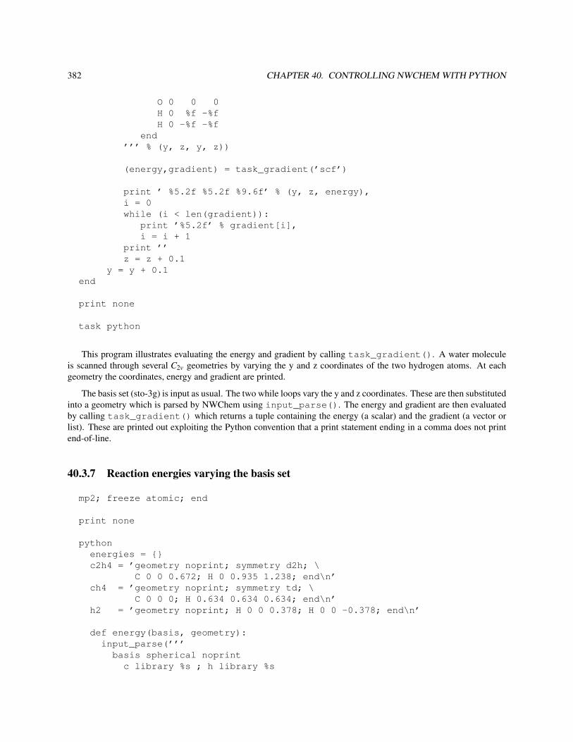
382 CHAPTER 40. CONTROLLING NWCHEM WITH PYTHON
O 0 0 0H 0 %f -%fH 0 -%f -%f
end’’’ % (y, z, y, z))
(energy,gradient) = task_gradient(’scf’)
print ’ %5.2f %5.2f %9.6f’ % (y, z, energy),i = 0while (i < len(gradient)):
print ’%5.2f’ % gradient[i],i = i + 1
print ’’z = z + 0.1
y = y + 0.1end
print none
task python
This program illustrates evaluating the energy and gradient by calling task_gradient(). A water moleculeis scanned through several C2v geometries by varying the y and z coordinates of the two hydrogen atoms. At eachgeometry the coordinates, energy and gradient are printed.
The basis set (sto-3g) is input as usual. The two while loops vary the y and z coordinates. These are then substitutedinto a geometry which is parsed by NWChem using input_parse(). The energy and gradient are then evaluatedby calling task_gradient() which returns a tuple containing the energy (a scalar) and the gradient (a vector orlist). These are printed out exploiting the Python convention that a print statement ending in a comma does not printend-of-line.
40.3.7 Reaction energies varying the basis set
mp2; freeze atomic; end
print none
pythonenergies = {}c2h4 = ’geometry noprint; symmetry d2h; \
C 0 0 0.672; H 0 0.935 1.238; end\n’ch4 = ’geometry noprint; symmetry td; \
C 0 0 0; H 0.634 0.634 0.634; end\n’h2 = ’geometry noprint; H 0 0 0.378; H 0 0 -0.378; end\n’
def energy(basis, geometry):input_parse(’’’
basis spherical noprintc library %s ; h library %s

40.3. EXAMPLES 383
end’’’ % (basis, basis))input_parse(geometry)return task_energy(’mp2’)
for basis in (’sto-3g’, ’6-31g’, ’6-31g*’, ’cc-pvdz’, ’cc-pvtz’):energies[basis] = 2*energy(basis, ch4) \
- 2*energy(basis, h2) - energy(basis, c2h4)if (ga_nodeid() == 0): print basis, ’ %8.6f’ % energies[basis]
end
task python
In this example the reaction energy for 2H2 +C2H4 → 2CH4 is evaluated using MP2 in several basis sets. Thegeometries are fixed, but could be re-optimized in each basis. To illustrate the useful associative arrays in Python, thereaction energies are put into the associative array energies — note its declaration at the top of the program.
40.3.8 Using the database
pythonrtdb_put("test_int2", 22)rtdb_put("test_int", [22, 10, 3], INT)rtdb_put("test_dbl", [22.9, 12.4, 23.908], DBL)rtdb_put("test_str", "hello", CHAR)rtdb_put("test_logic", [0,1,0,1,0,1], LOGICAL)rtdb_put("test_logic2", 0, LOGICAL)
rtdb_print(1)
print "test_str = ", rtdb_get("test_str")print "test_int = ", rtdb_get("test_int")print "test_in2 = ", rtdb_get("test_int2")print "test_dbl = ", rtdb_get("test_dbl")print "test_logic = ", rtdb_get("test_logic")print "test_logic2 = ", rtdb_get("test_logic2")
end
task python
This example illustrates how to access the database from Python.
40.3.9 Handling exceptions from NWChem
geometry; he 0 0 0; he 0 0 2; endbasis; he library 3-21g; endscf; maxiter 1; end
pythontry:

384 CHAPTER 40. CONTROLLING NWCHEM WITH PYTHON
task_energy(’scf’)except NWChemError, message:
print ’Error from NWChem ... ’, messageend
task python
The above test program shows how to handle exceptions generated by NWChem by forcing an SCF calculation onHe2 to fail due to insufficient iterations.
If an NWChem command fails it will raise the exception "NWChemError" (case sensitive) unless the error wasfatal. If the exception is not caught, then it will cause the entire Python program to terminate with an error. This Pythonprogram catches the exception, prints out the message, and then continues as if all was well since the exception hasbeen handled.
If your Python program detects an error, raise an unhandled exception. Do not call exit(1) since this maycircumvent necessary clean-up of the NWChem execution environment.
40.3.10 Accessing geometry information — a temporary hack
In an ideal world the geometry and basis set objects would have full Python wrappers, but until then a back-doorsolution will have to suffice. We’ve already seen how to use input_parse() to put geometry (and basis) data intoNWChem, so it only remains to get the geometry data back after it has been updated by a geometry optimzation orsome other operation.
The following Python procedure retrieves the coordinates in the same units as initially input for a geometry of agiven name. Its full source is included in the NWChem contrib directory.
def geom_get_coords(name):try:
actualname = rtdb_get(name)except NWChemError:
actualname = namecoords = rtdb_get(’geometry:’ + actualname + ’:coords’)units = rtdb_get(’geometry:’ + actualname + ’:user units’)if (units == ’a.u.’):
factor = 1.0elif (units == ’angstroms’):
factor = rtdb_get(’geometry:’+actualname+’:angstrom_to_au’)else:
raise NWChemError,’unknown units’i = 0while (i < len(coords)):
coords[i] = coords[i] / factori = i + 1
return coords
A geometry (see Section 6) with name NAME has its coordinates (in atomic units) stored in the database entrygeometry:NAME:coords. A minor wrinkle here is that indirection is possible (and used by the optimizers) so thatwe must first check if NAME actually points to another name. In the program this is done in the first try...exceptsequence. With the actual name of the geometry, we can get the coordinates. Any exceptions are passed up to the

40.3. EXAMPLES 385
caller. The rest of the code is just to convert back into the initial input units — only atomic units or Angstrøms arehandled in this simple example. Returned is a list of the atomic coordinates in the same units as your initial input.
The routine is used as follows
coords = geom_get_coords(’geometry’)
or, if you want better error handling
try:coords = geom_get_coords(’geometry’)
except NWChemError,message:print ’Coordinates for geometry not found ’, message
else:print coords
This is very dirty and definitely not supported from one release to another, but, browsing the output of rtdb_print()at the end of a calculation is a good way to find stuff. To be on safer ground, look in the programmers manual sincesome of the high-level routines do pass data via the database in a well-defined and supported manner. Be warned— you must be very careful if you try to modify data in the database. The input parser does many important thingsthat are not immediately apparent (e.g., ensure the geometry is consistent with the point group, mark the SCF as notconverged if the SCF options are changed, . . . ). Where at all possible your Python program should generate standardNWChem input and pass it to input_parse() rather than setting parameters directly in the database.
40.3.11 Scaning a basis exponent yet again — plotting and handling child processes
geometry units auO 0 0 0; H 0 1.430 -1.107; H 0 -1.430 -1.107
end
print none
pythonimport Gnuplot, time, signal
def energy_at_exponent(exponent):input_parse(’’’
basis noprintH library 3-21g; O library 3-21g; O d; %f 1.0
end’’’ % (exponent))return task_energy(’scf’)
data = []exponent = 0.5while exponent <= 0.6:
energy = energy_at_exponent(exponent)print ’ exponent = ’, exponent, ’ energy = ’, energydata = data + [[exponent,energy]]exponent = exponent + 0.02

386 CHAPTER 40. CONTROLLING NWCHEM WITH PYTHON
if (ga_nodeid() == 0):signal.signal(signal.SIGCHLD, signal.SIG_DFL)g = Gnuplot.Gnuplot()g(’set data style linespoints’)g.plot(data)time.sleep(30) # 30s to look at the plot
end
task python
This illustrates how to handle signals from terminating child processes and how to generate simple plots on UNIXsystems. The example from Section 40.3.3 is modified so that instead of writing the data to a file for subsequentvisualization, it is saved for subsequent visualization with Gnuplot (you’ll need both Gnuplot and the correspondingpackage for Python in your PYTHONPATH. Look at http://monsoon.harvard.edu/ mhagger/download).
The issue is that NWChem traps various signals from the O/S that usually indicate bad news in order to providebetter error handling and reliable clean-up of shared, parallel resources. One of these signals is SIGCHLD whichis generated whenever a child process terminates. If you want to create child processes within Python, then theNWChem handler for SIGCHLD must be replaced with the default handler. There seems to be no easy way to restorethe NWChem handler after the child has completed, but this should have no serious side effect.
40.4 Troubleshooting
Common problems with Python programs inside NWChem.
1. You get the message
0:python_input: indentation must be >= that of first line: 4
This indicates that NWChem thinks that a line is less indented than the first line. If this is not the case thenperhaps there is a tab in your input which NWChem treats as a single space character but appears to you as morespaces. Try running untabify in Emacs. The problem could also be the END directive that terminates thePYTHON compound directive — since Python also has an end statement. To avoid confusion the END directivefor NWChem must be at the start of the line.
2. Your program hangs or deadlocks — most likely you have a piece of code that is restricted to executing on asubset of the processors (perhaps just node 0) but is calling (perhaps indirectly) a function that must execute onall nodes.

Chapter 41
Interfaces to Other Programs
NWChem has interfaces to several different packages which are listed below. In general, the NWChem authors workwith the authors of the other packages to make sure that the interface works. However, any problems with the interfaceshould be reported to the [email protected] e-mail list.
41.1 DIRDYVTST— DIRect Dynamics for Variational Transition State The-ory
by Bruce C. Garrett,Environmental Molecular Sciences Laboratory,Pacific Northwest Laboratory, Richland, Washington
Yao-Yuan Chuang and Donald G. Truhlar,Department of Chemistry and Super Computer Institute,University of Minnesota, MN 55455-0431
and interfaced to NWChem by
Ricky A. Kendall,Scalable Computing Laboratory,Ames Laboratory and Iowa State University, Ames, IA 50011
Theresa L. Windus,Environmental Molecular Sciences Laboratory,Pacific Northwest Laboratory, Richland, Washington
If you use the DIRDYVTST portion of NWChem, please use following citation in addition to the usual NWChemcitation from Section 1:
DIRDYVTST, Yao-Yuan Chuang and Donald G. Truhlar, Department of Chemistry and Super ComputerInstitute, University of Minnesota; Ricky A. Kendall,Scalable Computing Laboratory, Ames Laboratoryand Iowa State University; Bruce C. Garrett and Theresa L. Windus, Environmental Molecular SciencesLaboratory, Pacific Northwest Laboratory.
387

388 CHAPTER 41. INTERFACES TO OTHER PROGRAMS
41.1.1 Introduction
By using DIRDYVTST, a user can carry out electronic structure calculations with NWChem and use the resultingenergies, gradients, and Hessians for direct dynamics calculations with POLYRATE. This program prepares the file30input for POLYRATE from NWChem electronic structure calculations of energies, gradients and Hessians at thereactant, product, and saddle point geometries and along the minimum energy path. Cartesian geometries for thereactants, products, and saddle points need to be input to this program; optimization of geometries is not performed inthis program. Note that DIRDYVTST is based on the DIRDYGAUSS program and is similar to two other programs:DDUTILITIES and GAUSSRATE. Users of this module are encouraged to read the POLYRATE manual since theywill need to create the file fu5 input to run calculations with POLYRATE.
Notes about the code:
Input. The code has been written to parallel, as much as possible, the POLYRATE code.
Output. There is one default output file for each DIRDYVTST run - .file30.
Integrators for following the reaction path. Currently the Euler and three Page-McIver (PM) methods are imple-mented. The PM methods are the local quadratic approximation (LQA), the corrected LQA (CLQA), and the cubic(CUBE) algorithm. The PM methods are implemented so that the Hessian can be reused at intermediate steps at whichonly the gradient is updated.
41.1.2 Files
Test runs are located in directories in $NWCHEM_TOP/QA/tests. Test runs are available for two systems: H +H2and OH +H2.
The H +H2 test uses the Euler integration method at the SCF/3-21G level of theory to calculate points along thereaction path. This test is located in the $NWCHEM_TOP/QA/tests/h3tr1 directory.
The OH +H2 test uses the Page-McIver CUBE algorithm to calculate points on the SCF/3-21G surface and doesadditional single point calculations at the SCF/6-31G* level of theory. This test is located in the $NWCHEM_TOP/QA/tests/oh3tr3directory.
Note: These tests are set up with SCF, however, other levels of theory can be used. The initial hessian calculationsat the reactants, products and saddle point can cause some problems when numerical hessians are required (especiallywhen there is symmetry breaking in the wavefunction).
41.1.3 Detailed description of the input
The input consists of keywords for NWChem and keywords related to POLYRATE input. The first set of inputs are forNWChem with the general input block of the form:
DIRDYVTST [autosym [real tol default 1d-2] | noautosym][THEORY <string theory> [basis <string basis default "ao basis">] \
[ecp <string ecp>] [input <string input>]][SPTHEORY <string theory> [basis <string basis default "ao basis">] \
[ecp <string ecp>] [input <string input>]]...
END

41.1. DIRDYVTST — DIRECT DYNAMICS FOR VARIATIONAL TRANSITION STATE THEORY 389
Use of symmetry
The use of symmetry in the calculation is controlled by the keyword autosym | noautosym which is used asdescribed in the geometry directive (see Section 6). Autosym is on by default. A couple words of warning here.The tolerance related to autosym can cause problems when taking the initial step off of the transition state. If thetolerance is too large and the initial step relatively small, the resulting geometry will be close to a higher symmetrythan is really wanted and the molecule will be symmetrized into the higher symmetry. To check this, the code printsout the symmetry at each geometry along the path. It is up to the user to check the symmetry and make sure that it isthe required one. In preverse cases, the user may need to turn autosym off (noautosym) if changing the tolerancedoesn’t produce the desired results. In the case that autosym is used, the user does not need to worry about the differentalignment of the molecule between NWChem and POLYRATE, this is taken care of internally in the DIRDYVTSTmodule.
Basis specification
The basis name on the theory or sptheory directive is that specified on a basis set directive (see Section 7) and not thename of a standard basis in the library. If not specified, the basis set for the sptheory defaults to the theory basis whichdefaults to "ao basis".
Effective core potentials
If an effective core potential is specified in the usual fashion (see Section 8) outside of the DIRDYVTST input thenthis will be used in all calculations. If an alternative ECP name (the name specified on the ECP directive in the samemanner as done for basis sets) is specified on one of the theory directives, then this ECP will be used in preference forthat level of theory.
General input strings
For many purposes, the ability to specify the theory, basis and effective core potential is adequate. All of the optionsfor each theory are determined from their independent input blocks. However, if the same theory (e.g., DFT) is tobe used with different options for theory and sptheory, then the general input strings must be used. These strings areprocessed as NWChem input each time the theoretical calculation is invoked. The strings may contain any NWCheminput, except for options pertaining to DIRDYVTST and the task directive. The intent is that the strings be used just tocontrol the options pertaining to the theory being used.
A word of caution. Be sure to check that the options are producing the desired results. Since the NWChemdatabase is persistent, the input strings should fully define the calculation you wish to have happen.
For instance, if the theory model is DFT/LDA/3-21g and the sptheory model is DFT/B3LYP/6-311g**, theDIRDYVTST input might look like this
dirdyvtsttheory dft basis 3-21g input "dft\; xc\; end"sptheory dft basis 6-311g** input "dft\; xc b3lyp\; end"....
end
The empty XC directive restores the default LDA exchange-correlation option (see Section 11.3). Note that semi-colons and other quotation marks inside the input string must be preceded by a backslash to avoid special interpretation.

390 CHAPTER 41. INTERFACES TO OTHER PROGRAMS
POLYRATE related options
These keyword options are simlar to the POLYRATE input format, except there are no ENERGETICS, OPTIMIZA-TION, SECOND, TUNNELING, and RATE sections.
GENERAL section The GENERAL section has the following format:
*GENERAL[TITLE <string title>]ATOMS
<integer num> <string tag> [<real mass>]...
END[SINGLEPOINT][SAVEFILE (vecs || hess || spc)
Descriptions
TITLE is a keyword that allows the user to input a description of the calculation. In this version, the user can onlyhave a single-line description.
For example: TITLE Calculation of D + HCl reaction
ATOMS is a list keyword that is used to input a list of the atoms. It is similar to POLYRATE in that the order ofthe atom and the atomic symbol are required in a single line. If isotope of the element is considered then the atomicmass is required in units of amu.
For example:
ATOMS1 H 2.0142 H3 Cl
END
SINGLEPOINT is a keyword that specifies that a single point calculation is to be performed at the reactants,products and saddle point geometries. The type of single point calculation is specified in the sptheory line.
SAVEFILE is a keyword that specifies that NWChem files are to be saved. Allowed values of variable inputto SAVEFILE are vecs, hess, and spc for saving the files base theory movecs, base theory hessian and singlepointcalculation movecs.
REACT1, REACT2, PROD1, PROD2, and START sections These sections have the following format:
*(REACT1 || REACT2 || PROD1 || PROD2 || START)GEOM
<integer num> <real x y z>...
ENDSPECIES (ATOMIC || LINRP || NONLINRP || LINTS || NONLINTS default NONLINRP)

41.1. DIRDYVTST — DIRECT DYNAMICS FOR VARIATIONAL TRANSITION STATE THEORY 391
REACT1 and REACT2 are input for each of the reactants and PROD1 and PROD2 are input for each of theproducts. REACT1 and PROD1 are required. START is the input for the transition state if one exists, or starting pointto follow downhill the MEP.
Descriptions
GEOM is a list keyword that indicates the geometry of the molecule in Cartesian coordinates with atomic unit.
For example:
GEOM1 0.0 0.0 0.02 0.0 0.0 1.5
END
SPECIES is a variable keyword that indicates the type of the molecule. Options are: ATOMIC (atomic reactantor product), LINRP (linear reactant or product), NONLINRP (nonlinear reactant or product), LINTS (linear transitionstate), and NONLINTS (nonlinear transition state).
For example: SPECIES atomic
PATH section The Path section has the format:
*PATH[SCALEMASS <real scalemass default 1.0>][SSTEP <real sstep default 0.01>][SSAVE <real ssave default 0.1>][SHESS <real shess default SSAVE>][SLP <real slp default 1.0>][SLM <real slm default -1.0>][SIGN (REACTANT || PRODUCT default REACTANT)][INTEGRA (EULER || LQA || CLQA || CUBE default EULER)][PRINTFREQ (on || off default off)]
Descriptions
SCALEMASS is a variable keyword that indicates the arbitrary mass (in amu) used for mass-scaled Cartesiancoordinates. This is the variable called mu in published papers. Normally, this is taken as either 1.0 amu or, forbimolecular reactions, as the reduced mass of relative translation of the reactants.
SSTEP is a variable keyword that indicates the numerical step size (in bohrs) for the gradient grid. This is the stepsize for following the minimum energy path.
SSAVE is a variable keyword that indicates the numerical step size (in bohrs) for saving the Hessian grid. At eachsave point the potential and its first and second derivatives are recalculated and written to the .file30 file. For example,if SSTEP=0.01 and SSAVE=0.1, then the potential information is written to .file30 every 10 steps along the gradientgrid.
SHESS is a variable keyword that indicates the numerical step size (in bohrs) for recomputing the Hessian whenusing a Page-McIver integrator (e.g., LQA, CLQA, or CUBE). For Euler integration SHESS = SSAVE. For interme-diate points along the gradient grid, the Hessian matrix from the last Hessian calculation is reused. For example, ifSSTEP=0.01 and SHESS=0.05, then the Hessian matrix is recomputed every 5 steps along the gradient grid.
SLP is a variable keyword that indicates the positive limit of the reaction coordinate (in bohrs).

392 CHAPTER 41. INTERFACES TO OTHER PROGRAMS
SLM is a variable keyword that indicates the negative limit of the reaction coordinate (in bohrs).
SIGN is a variable keyword used to ensure the conventional definition of the sign of s, s < 0 for the reactant sideand s > 0 for the product side, is followed. PRODUCT should be used if the eigenvector at the saddle point pointstoward the product side and REACTANT if the eigenvector points toward the reactant side.
INTEGRA is a variable keyword that indicates the integration method used to follow the reaction path. Optionsare: EULER, LQA, CLQA, and CUBE.
PRINTFREQ is a variable keyword that indicates that projected frequencies and eigenvectors will be printed alongthe MEP.
Restart
DIRDYVTST calculations should be restarted through the normal NWChem mechanism (See Section 5.1). The userneeds to change the start directive to a restart directive and get rid of any information that will overwriteimportant information in the RTDB. The file.db and file.file30 need to be available for the calculation torestart properly.
Example
This is an example that creates the file30 file for POLYRATE for H +H2. Note that the multiplicity is that of theentire supermolecule, a doublet. In this example, the initial energies, gradients, and Hessians are calculated at theUHF/3-21G level of theory and the singlepoint calculations are calculated at the MP2/cc-pVDZ level of theory with atighter convergence threshold than the first SCF.
start h3test
basish library 3-21G
end
basis singlepointh library cc-pVDZ
end
scfuhfdoubletthresh 1.0e-6
end
dirdyvtst autosym 0.001theory scf input "scf\; uhf\; doublet\; thresh 1.0e-06\; end"sptheory mp2 basis singlepoint input \
"scf\; uhf\; doublet\; thresh 1.0e-07\; end"
*GENERALTITLE
Test run: H+H2 reaction, Page-McIver CLQA algorithm, no restart
ATOMS

41.1. DIRDYVTST — DIRECT DYNAMICS FOR VARIATIONAL TRANSITION STATE THEORY 393
1 H2 H3 H
END
SINGLEPOINT
*REACT1GEOM
1 0.0 0.0 0.02 0.0 0.0 1.3886144
END
SPECIES LINRP
*REACT2GEOM
3 0.0 0.0 190.3612132END
SPECIES ATOMIC
*PROD2GEOM
1 0.0 0.0 190.3612132END
SPECIES ATOMIC
*PROD1
GEOM2 0.0 0.0 1.38861443 0.0 0.0 0.0
END
SPECIES LINRP
*START
GEOM1 0.0 0.0 -1.765319732 0.0 0.0 0.03 0.0 0.0 1.76531973
END
SPECIES LINTS
*PATHSSTEP 0.05SSAVE 0.05

394 CHAPTER 41. INTERFACES TO OTHER PROGRAMS
SLP 0.50SLM -0.50SCALEMASS 0.6718993INTEGRA CLQA
end
task dirdyvtst

Chapter 42
Acknowledgments
This work was supported by funds from the Environmental and Molecular Sciences Laboratory Construction Projectat Pacific Northwest National Laboratory. Development of some of the parallel programming tools and algorithmsemployed by NWChem was performed under the auspices of the High Performance Computing and CommunicationsProgram of the Mathematical, Information, and Computational Sciences Division, U.S. Department of Energy. PacificNorthwest National Laboratory is operated by Battelle Memorial Institute for the U.S. Department of Energy underContract DE-AC05-76RL01830.
395

396 CHAPTER 42. ACKNOWLEDGMENTS

Appendix A
Standard Basis Sets
Basis sets and effective core potentials were obtained (1/1/2002) from the Extensible Computational Chemistry En-vironment (ECCE) Basis Set Database, as developed and distributed by the Molecular Science Computing Facility,Environmental and Molecular Sciences Laboratory which is part of the Pacific Northwest National Laboratory, P.O.Box 999, Richland, Washington 99352, USA, and is funded by the U.S. Department of Energy. The Pacific NorthwestNational Laboratory is a multi-program laboratory operated by Battelle Memorial Institute for the U.S. Departmentof Energy under contract DE-AC05-76RL01830. Contact David Feller ([email protected]) or Deborah Gracio([email protected]) for further information.
The names in the NWChem library are consistent with those in the ECCE database and thus may include spaces.The standard NWChem input routines require that strings including spaces are enclosed in quotation marks ("...")or that blanks are escaped with a backslash. As a convenience, basis set names may also have the blanks replaced withunderscores. Thus, the following all yield the same basis set for oxygen
oxygen library "DZP + Diffuse (Dunning)"oxygen library DZP\ +\ Diffuse\ (Dunning)oxygen library DZP_+_Diffuse_(Dunning)
Case may be ignored when specifying basis set names, but otherwise names should be specified exactly as providedbelow. A good method is just to cut/paste from the WWW pages since they were generated electronically from thelibrary source.
Errors found in the basis set library of NWChem version 4.4 have been corrected in the current library of NWChemversion 4.6. The changes are listed below:
1. Basis Set "Stuttgart RLC ECP"Element: IEffective core potential has been changed and now conforms to the published from by Bergner et al. (Mol. Phys.1993).
Errors found in the basis set library of NWChem version 4.0 have been corrected in the current library of NWChemversion 4.1. The changes are listed below:
1. Basis Set "aug-cc-pVTZ"Element: BrCorrection of the diffuse s-exponent from 0.041601 to 0.045593.
397
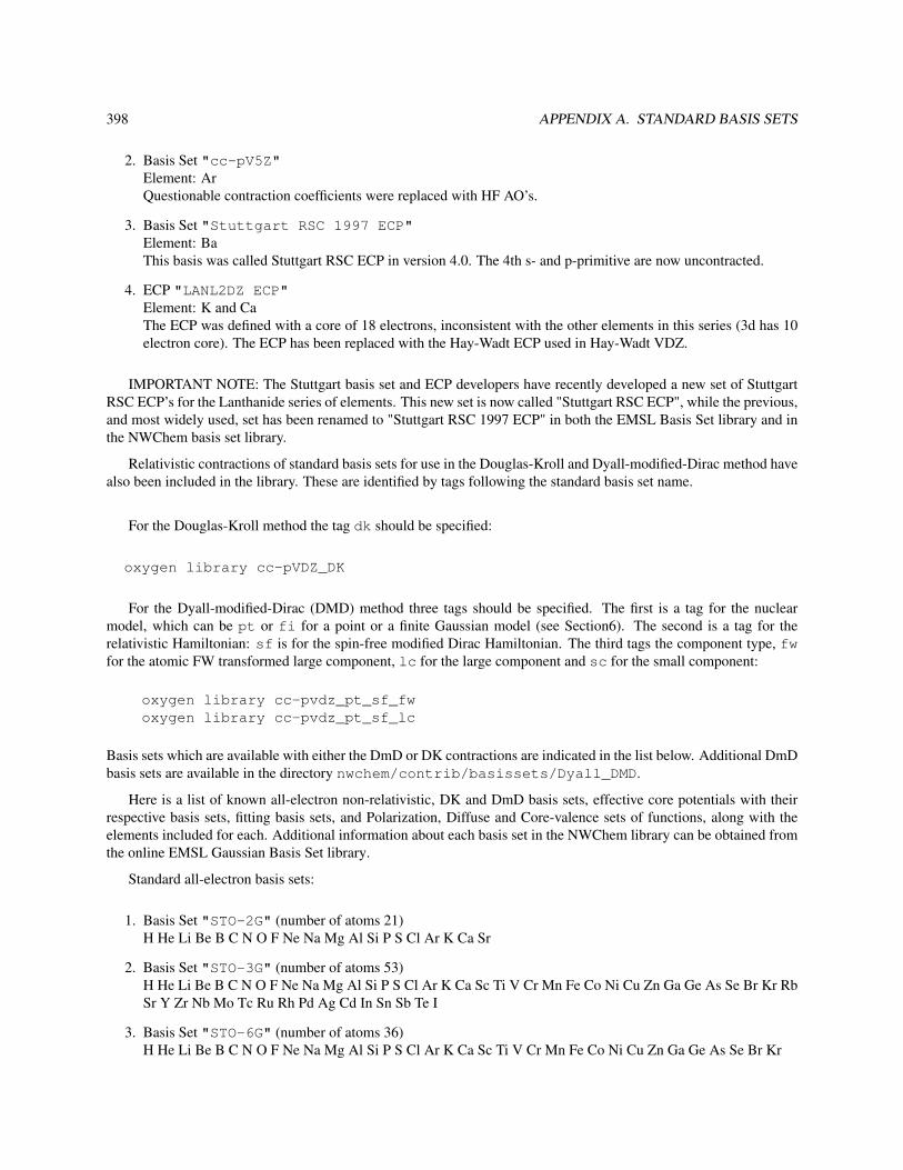
398 APPENDIX A. STANDARD BASIS SETS
2. Basis Set "cc-pV5Z"Element: ArQuestionable contraction coefficients were replaced with HF AO’s.
3. Basis Set "Stuttgart RSC 1997 ECP"Element: BaThis basis was called Stuttgart RSC ECP in version 4.0. The 4th s- and p-primitive are now uncontracted.
4. ECP "LANL2DZ ECP"Element: K and CaThe ECP was defined with a core of 18 electrons, inconsistent with the other elements in this series (3d has 10electron core). The ECP has been replaced with the Hay-Wadt ECP used in Hay-Wadt VDZ.
IMPORTANT NOTE: The Stuttgart basis set and ECP developers have recently developed a new set of StuttgartRSC ECP’s for the Lanthanide series of elements. This new set is now called "Stuttgart RSC ECP", while the previous,and most widely used, set has been renamed to "Stuttgart RSC 1997 ECP" in both the EMSL Basis Set library and inthe NWChem basis set library.
Relativistic contractions of standard basis sets for use in the Douglas-Kroll and Dyall-modified-Dirac method havealso been included in the library. These are identified by tags following the standard basis set name.
For the Douglas-Kroll method the tag dk should be specified:
oxygen library cc-pVDZ_DK
For the Dyall-modified-Dirac (DMD) method three tags should be specified. The first is a tag for the nuclearmodel, which can be pt or fi for a point or a finite Gaussian model (see Section6). The second is a tag for therelativistic Hamiltonian: sf is for the spin-free modified Dirac Hamiltonian. The third tags the component type, fwfor the atomic FW transformed large component, lc for the large component and sc for the small component:
oxygen library cc-pvdz_pt_sf_fwoxygen library cc-pvdz_pt_sf_lc
Basis sets which are available with either the DmD or DK contractions are indicated in the list below. Additional DmDbasis sets are available in the directory nwchem/contrib/basissets/Dyall_DMD.
Here is a list of known all-electron non-relativistic, DK and DmD basis sets, effective core potentials with theirrespective basis sets, fitting basis sets, and Polarization, Diffuse and Core-valence sets of functions, along with theelements included for each. Additional information about each basis set in the NWChem library can be obtained fromthe online EMSL Gaussian Basis Set library.
Standard all-electron basis sets:
1. Basis Set "STO-2G" (number of atoms 21)H He Li Be B C N O F Ne Na Mg Al Si P S Cl Ar K Ca Sr
2. Basis Set "STO-3G" (number of atoms 53)H He Li Be B C N O F Ne Na Mg Al Si P S Cl Ar K Ca Sc Ti V Cr Mn Fe Co Ni Cu Zn Ga Ge As Se Br Kr RbSr Y Zr Nb Mo Tc Ru Rh Pd Ag Cd In Sn Sb Te I
3. Basis Set "STO-6G" (number of atoms 36)H He Li Be B C N O F Ne Na Mg Al Si P S Cl Ar K Ca Sc Ti V Cr Mn Fe Co Ni Cu Zn Ga Ge As Se Br Kr

399
4. Basis Set "STO-3G*" (number of atoms 18)H He Li Be B C N O F Ne Na Mg Al Si P S Cl Ar
5. Basis Set "3-21G" (number of atoms 55)H He Li Be B C N O F Ne Na Mg Al Si P S Cl Ar K Ca Sc Ti V Cr Mn Fe Co Ni Cu Zn Ga Ge As Se Br Kr RbSr Y Zr Nb Mo Tc Ru Rh Pd Ag Cd In Sn Sb Te I Xe Cs
6. Basis Set "3-21++G" (number of atoms 18)H He Li Be B C N O F Ne Na Mg Al Si P S Cl Ar
7. Basis Set "3-21G*" (number of atoms 18)H He Li Be B C N O F Ne Na Mg Al Si P S Cl Ar
8. Basis Set "3-21++G*" (number of atoms 18)H He Li Be B C N O F Ne Na Mg Al Si P S Cl Ar
9. Basis Set "3-21GSP" (number of atoms 18)H He Li Be B C N O F Ne Na Mg Al Si P S Cl Ar
10. Basis Set "4-22GSP" (number of atoms 18)H He Li Be B C N O F Ne Na Mg Al Si P S Cl Ar
11. Basis Set "4-31G" (number of atoms 13)H He Li Be B C N O F Ne P S Cl
12. Basis Set "6-31G" (number of atoms 30)H He Li Be B C N O F Ne Na Mg Al Si P S Cl Ar K Ca Sc Ti V Cr Mn Fe Co Ni Cu Zn
13. Basis Set "6-31G*" (number of atoms 30)H He Li Be B C N O F Ne Na Mg Al Si P S Cl Ar K Ca Sc Ti V Cr Mn Fe Co Ni Cu Zn
14. Basis Set "6-31G**" (number of atoms 30)H He Li Be B C N O F Ne Na Mg Al Si P S Cl Ar K Ca Sc Ti V Cr Mn Fe Co Ni Cu Zn
15. Basis Set "6-31++G" (number of atoms 20)H He Li Be B C N O F Ne Na Mg Al Si P S Cl Ar K Ca
16. Basis Set "6-31++G*" (number of atoms 18)H He Li Be B C N O F Ne Na Mg Al Si P S Cl Ar
17. Basis Set "6-31++G**" (number of atoms 18)H He Li Be B C N O F Ne Na Mg Al Si P S Cl Ar
18. Basis Set "6-31+G*" (number of atoms 18)H He Li Be B C N O F Ne Na Mg Al Si P S Cl Ar
19. Basis Set "6-31G(3df,3pd)" (number of atoms 18)H He Li Be B C N O F Ne Na Mg Al Si P S Cl Ar
20. Basis Set "6-31G-Blaudeau" (number of atoms 2)K Ca
21. Basis Set "6-31G*-Blaudeau" (number of atoms 2)K Ca
22. Basis Set "6-311G" (number of atoms 25)H He Li Be B C N O F Ne Na Mg Al Si P S Cl Ar Ga Ge As Se Br Kr I

400 APPENDIX A. STANDARD BASIS SETS
23. Basis Set "6-311G*" (number of atoms 25)H He Li Be B C N O F Ne Na Mg Al Si P S Cl Ar Ga Ge As Se Br Kr I
24. Basis Set "6-311G**" (number of atoms 25)H He Li Be B C N O F Ne Na Mg Al Si P S Cl Ar Ga Ge As Se Br Kr I
25. Basis Set "6-311++G**" (number of atoms 10)H He Li Be B C N O F Ne
26. Basis Set "6-311++G(2d,2p)" (number of atoms 20)H He Li Be B C N O F Ne Na Mg Al Si P S Cl Ar K Ca
27. Basis Set "6-311G(2df,2pd)" (number of atoms 12)H He Li Be B C N O F Ne K Ca
28. Basis Set "6-311+G*" (number of atoms 10)H He Li Be B C N O F Ne
29. Basis Set "6-311++G(3df,3pd)" (number of atoms 18)H He Li Be B C N O F Ne Na Mg Al Si P S Cl Ar
30. Basis Set "MINI (Huzinaga)" (number of atoms 20)H He Li Be B C N O F Ne Na Mg Al Si P S Cl Ar K Ca
31. Basis Set "MINI (Scaled)" (number of atoms 20)H He Li Be B C N O F Ne Na Mg Al Si P S Cl Ar K Ca
32. Basis Set "MIDI (Huzinaga)" (number of atoms 19)H He Li Be B C N O F Ne Na Al Si P S Cl Ar K Cs
33. Basis Set "MIDI!" (number of atoms 11)H C N O F Si P S Cl Br I
34. Basis Set "SV (Dunning-Hay)" (number of atoms 9)H Li Be B C N O F Ne
35. Basis Set "SVP (Dunning-Hay)" (number of atoms 9)H Li Be B C N O F Ne
36. Basis Set "SVP + Diffuse (Dunning-Hay)" (number of atoms 9)H Li Be B C N O F Ne
37. Basis Set "TZ (Dunning)" (number of atoms 8)H Li B C N O F Ne
38. Basis Set "Chipman DZP + Diffuse" (number of atoms 6)H B C N O F
39. Basis Set "DZ (Dunning)" (number of atoms 13)H Li B C N O F Ne Al Si P S Cl
40. Basis Set "DZP (Dunning)" (number of atoms 13)H Li B C N O F Ne Al Si P S Cl
41. Basis Set "DZP + Diffuse (Dunning)" (number of atoms 7)H B C N O F Ne

401
42. Basis Set "cc-pVDZ" (number of atoms 24)H He Li Be B C N O F Ne Na Mg Al Si P S Cl Ar Ga Ge As Se Br Kr
43. Basis Set "cc-pVTZ" (number of atoms 24)H He Li Be B C N O F Ne Na Mg Al Si P S Cl Ar Ga Ge As Se Br Kr
44. Basis Set "cc-pVQZ" (number of atoms 22)H He Li Be B C N O F Ne Na Mg Al Si P S Cl Ar Ga Ge As Se
45. Basis Set "cc-pV5Z" (number of atoms 24)H He Li Be B C N O F Ne Na Mg Al Si P S Cl Ar Ga Ge As Se Br Kr
46. Basis Set "cc-pV6Z" (number of atoms 14)H He B C N O F Ne Al Si P S Cl Ar
47. Basis Set "pV6Z" (number of atoms 4)H C N O
48. Basis Set "cc-pVDZ(seg-opt)" (number of atoms 24)H He Li Be B C N O F Ne Na Mg Al Si P S Cl Ar Ga Ge As Se Br Kr
49. Basis Set "cc-pVTZ(seg-opt)" (number of atoms 24)H He Li Be B C N O F Ne Na Mg Al Si P S Cl Ar Ga Ge As Se Br Kr
50. Basis Set "cc-pVQZ(seg-opt)" (number of atoms 4)H He C O
51. Basis Set "cc-pCVDZ" (number of atoms 12)Li Be B C N O F Ne Na Mg Si Cl
52. Basis Set "cc-pCVTZ" (number of atoms 13)Li Be B C N O F Ne Na Mg Si P Cl
53. Basis Set "cc-pCVQZ" (number of atoms 13)Li Be B C N O F Ne Na Mg Si P Cl
54. Basis Set "cc-pCV5Z" (number of atoms 8)B C N O F Ne Na Mg
55. Basis Set "cc-pCV6Z" (number of atoms 1)O
56. Basis Set "aug-cc-pVDZ" (number of atoms 24)H He Li Be B C N O F Ne Na Mg Al Si P S Cl Ar Ga Ge As Se Br Kr
57. Basis Set "aug-cc-pVTZ" (number of atoms 23)H He Li Be B C N O F Ne Na Mg Al Si P S Cl Ar Ga Ge As Se Br
58. Basis Set "aug-cc-pVQZ" (number of atoms 24)H He Li Be B C N O F Ne Na Mg Al Si P S Cl Ar Ga Ge As Se Br Kr
59. Basis Set "aug-cc-pV5Z" (number of atoms 20)H He B C N O F Ne Al Si P S Cl Ar Ga Ge As Se Br Kr
60. Basis Set "aug-cc-pV6Z" (number of atoms 14)H He B C N O F Ne Al Si P S Cl Ar

402 APPENDIX A. STANDARD BASIS SETS
61. Basis Set "aug-cc-pCVDZ" (number of atoms 7)B C N O F Na Mg
62. Basis Set "aug-cc-pCVTZ" (number of atoms 8)B C N O F Ne Na Mg
63. Basis Set "aug-cc-pCVQZ" (number of atoms 6)B C N O F Ne
64. Basis Set "aug-cc-pCV5Z" (number of atoms 5)B C N O F
65. Basis Set "d-aug-cc-pVDZ" (number of atoms 8)H He B C N O F Ne
66. Basis Set "d-aug-cc-pVTZ" (number of atoms 8)H He B C N O F Ne
67. Basis Set "d-aug-cc-pVQZ" (number of atoms 8)H He B C N O F Ne
68. Basis Set "d-aug-cc-pV5Z" (number of atoms 8)H He B C N O F Ne
69. Basis Set "d-aug-cc-pV6Z" (number of atoms 5)H B C N O
70. Basis Set "cc-pV(D+d)Z" (number of atoms 6)Al Si P S Cl Ar
71. Basis Set "cc-pV(T+d)Z" (number of atoms 6)Al Si P S Cl Ar
72. Basis Set "cc-pV(Q+d)Z" (number of atoms 6)Al Si P S Cl Ar
73. Basis Set "cc-pV(5+d)Z" (number of atoms 6)Al Si P S Cl Ar
74. Basis Set "cc-pV(6+d)Z" (number of atoms 6)Al Si P S Cl Ar
75. Basis Set "aug-cc-pV(D+d)Z" (number of atoms 6)Al Si P S Cl Ar
76. Basis Set "aug-cc-pV(T+d)Z" (number of atoms 6)Al Si P S Cl Ar
77. Basis Set "aug-cc-pV(Q+d)Z" (number of atoms 6)Al Si P S Cl Ar
78. Basis Set "aug-cc-pV(5+d)Z" (number of atoms 6)Al Si P S Cl Ar
79. Basis Set "aug-cc-pV(6+d)Z" (number of atoms 6)Al Si P S Cl Ar

403
80. Basis Set "Feller Misc. CVDZ" (number of atoms 1)K
81. Basis Set "Feller Misc. CVTZ" (number of atoms 1)K
82. Basis Set "Feller Misc. CVQZ" (number of atoms 1)K
83. Basis Set "GAMESS VTZ" (number of atoms 16)H Be B C N O F Ne Na Mg Al Si P S Cl Ar
84. Basis Set "GAMESS PVTZ" (number of atoms 8)H Be B C N O F Ne
85. Basis Set "Partridge Uncontr. 1" (number of atoms 36)Li Be B C N O F Ne Na Mg Al Si P S Cl Ar K Ca Sc Ti V Cr Mn Fe Co Ni Cu Zn Ga Ge As Se Br Kr Rb Sr
86. Basis Set "Partridge Uncontr. 2" (number of atoms 34)Li Be B C N O F Ne Na Mg Al Si P S Cl Ar K Ca Sc Ti V Cr Mn Fe Co Ni Cu Zn Ga Ge As Se Br Kr
87. Basis Set "Partridge Uncontr. 3" (number of atoms 28)Li Be B C N O F Ne Na Mg Al Si P S Cl Ar K Ca Sc Ti V Cr Mn Fe Co Ni Cu Zn
88. Basis Set "Ahlrichs VDZ" (number of atoms 36)H He Li Be B C N O F Ne Na Mg Al Si P S Cl Ar K Ca Sc Ti V Cr Mn Fe Co Ni Cu Zn Ga Ge As Se Br Kr
89. Basis Set "Ahlrichs pVDZ" (number of atoms 36)H He Li Be B C N O F Ne Na Mg Al Si P S Cl Ar K Ca Sc Ti V Cr Mn Fe Co Ni Cu Zn Ga Ge As Se Br Kr
90. Basis Set "Ahlrichs VTZ" (number of atoms 36)H He Li Be B C N O F Ne Na Mg Al Si P S Cl Ar K Ca Sc Ti V Cr Mn Fe Co Ni Cu Zn Ga Ge As Se Br Kr
91. Basis Set "Ahlrichs TZV" (number of atoms 34)Li Be B C N O F Ne Na Mg Al Si P S Cl Ar K Ca Sc Ti V Cr Mn Fe Co Ni Cu Zn Ga Ge As Se Br Kr
92. Basis Set "Binning/Curtiss SV" (number of atoms 6)Ga Ge As Se Br Kr
93. Basis Set "Binning/Curtiss VTZ" (number of atoms 6)Ga Ge As Se Br Kr
94. Basis Set "Binning/Curtiss SVP" (number of atoms 6)Ga Ge As Se Br Kr
95. Basis Set "Binning/Curtiss VTZP" (number of atoms 6)Ga Ge As Se Br Kr
96. Basis Set "McLean/Chandler VTZ" (number of atoms 8)Na Mg Al Si P S Cl Ar
97. Basis Set "SV + Rydberg (Dunning-Hay)" (number of atoms 9)H Li Be B C N O F Ne
98. Basis Set "SVP + Rydberg (Dunning-Hay)" (number of atoms 9)H Li Be B C N O F Ne

404 APPENDIX A. STANDARD BASIS SETS
99. Basis Set "SVP + Diffuse + Rydberg" (number of atoms 9)H Li Be B C N O F Ne
100. Basis Set "DZ + Rydberg (Dunning)" (number of atoms 12)H B C N O F Ne Al Si P S Cl
101. Basis Set "DZP + Rydberg (Dunning)" (number of atoms 12)H B C N O F Ne Al Si P S Cl
102. Basis Set "DZ + Double Rydberg (Dunning-Hay)" (number of atoms 12)H B C N O F Ne Al Si P S Cl
103. Basis Set "SV + Double Rydberg (Dunning-Hay)" (number of atoms 9)H Li Be B C N O F Ne
104. Basis Set "Wachters+f" (number of atoms 9)Sc Ti V Cr Mn Fe Co Ni Cu
105. Basis Set "Bauschlicher ANO" (number of atoms 9)Sc Ti V Cr Mn Fe Co Ni Cu
106. Basis Set "NASA Ames ANO" (number of atoms 12)H B C N O F Ne Al P Ti Fe Ni
107. Basis Set "NASA Ames cc-pVTZ" (number of atoms 1)Ti
108. Basis Set "NASA Ames cc-pVQZ" (number of atoms 1)Ti
109. Basis Set "NASA Ames cc-pV5Z" (number of atoms 1)Ti
110. Basis Set "NASA Ames cc-pCVTZ" (number of atoms 1)Ti
111. Basis Set "NASA Ames cc-pCVQZ" (number of atoms 1)Ti
112. Basis Set "NASA Ames cc-pCV5Z" (number of atoms 1)Ti
113. Basis Set "Sadlej pVTZ" (number of atoms 19)H Li Be C N O F Na Mg Si P S Cl K Ca Br Rb Sr I
114. Basis Set "WTBS" (number of atoms 84)He Li Be B C N O F Ne Na Mg Al Si P S Cl Ar K Ca Sc Ti V Cr Mn Fe Co Ni Cu Zn Ga Ge As Se Br Kr RbSr Y Zr Nb Mo Tc Ru Rh Pd Ag Cd In Sn Sb Te I Xe Cs Ba La Ce Pr Pm Sm Eu Gd Tb Dy Ho Er Tm Yb LuHf Ta W Re Os Ir Pt Au Hg Tl Pb Bi Po At Rn
Resolution of Identity (RI) fitting basis sets:
1. Basis Set "cc-pVDZ-fit2-1" (number of atoms 10)H He Li Be B C N O F Ne
2. Basis Set "cc-pVTZ-fit2-1" (number of atoms 10)H He Li Be B C N O F Ne

405
Density functional specific basis sets:
1. Basis Set "DZVP (DFT Orbital)" (number of atoms 54)H He Li Be B C N O F Ne Na Mg Al Si P S Cl Ar K Ca Sc Ti V Cr Mn Fe Co Ni Cu Zn Ga Ge As Se Br Kr RbSr Y Zr Nb Mo Tc Ru Rh Pd Ag Cd In Sn Sb Te I Xe
2. Basis Set "DZVP2 (DFT Orbital)" (number of atoms 25)H He Li Be B C N O F Al Si P S Cl Ar Sc Ti V Cr Mn Fe Co Ni Cu Zn
3. Basis Set "TZVP (DFT Orbital)" (number of atoms 11)H C N O F Al Si P S Cl Ar
Density functional Coulomb and Exchange fitting basis sets:
1. Basis Set "DGauss A1 DFT Coulomb Fitting" (number of atoms 54)H He Li Be B C N O F Ne Na Mg Al Si P S Cl Ar K Ca Sc Ti V Cr Mn Fe Co Ni Cu Zn Ga Ge As Se Br Kr RbSr Y Zr Nb Mo Tc Ru Rh Pd Ag Cd In Sn Sb Te I Xe
2. Basis Set "DGauss A1 DFT Exchange Fitting" (number of atoms 54)H He Li Be B C N O F Ne Na Mg Al Si P S Cl Ar K Ca Sc Ti V Cr Mn Fe Co Ni Cu Zn Ga Ge As Se Br Kr RbSr Y Zr Nb Mo Tc Ru Rh Pd Ag Cd In Sn Sb Te I Xe
3. Basis Set "DGauss A2 DFT Coulomb Fitting" (number of atoms 28)H He Li Be B C N O F Ne Na Mg Al Si P S Cl Ar Sc Ti V Cr Mn Fe Co Ni Cu Zn
4. Basis Set "DGauss A2 DFT Exchange Fitting" (number of atoms 64)H He Li Be B C N O F Ne Na Mg Al Si P S Cl Ar Sc Ti V Cr Mn Fe Co Ni Cu Zn
5. Basis Set "Ahlrichs Coulomb Fitting" (number of atoms 70)H He Li Be B C N O F Ne Na Mg Al Si P S Cl Ar K Ca Sc Ti V Cr Mn Fe Co Ni Cu Zn Ga Ge As Se Br Kr RbSr Y Zr Nb Mo Tc Ru Rh Pd Ag Cd In Sn Sb Te I Xe Cs Ba Hf Ta W Re Os Ir Pt Au Hg Tl Pb Bi Po At
6. Basis Set "DeMon Coulomb Fitting" (number of atoms 54)H He Li Be B C N O F Ne Na Mg Al Si P S Cl Ar K Ca Sc Ti V Cr Mn Fe Co Ni Cu Zn Ga Ge As Se Br Kr RbSr Y Zr Nb Mo Tc Ru Rh Pd Ag Cd In Sn Sb Te I Xe
Effective core potentials and their respective basis sets:
1. Basis Set "Hay-Wadt MB (n+1) ECP" (number of atoms 32)K Ca Sc Ti V Cr Mn Fe Co Ni Cu Rb Sr Y Zr Nb Mo Tc Ru Rh Pd Ag Cs Ba La Ta W Re Os Ir Pt Au
2. ECP "Hay-Wadt MB (n+1) ECP" (number of atoms 32)K Ca Sc Ti V Cr Mn Fe Co Ni Cu Rb Sr Y Zr Nb Mo Tc Ru Rh Pd Ag Cs Ba La Ta W Re Os Ir Pt Au
3. Basis Set "Hay-Wadt VDZ (n+1) ECP" (number of atoms 32)K Ca Sc Ti V Cr Mn Fe Co Ni Cu Rb Sr Y Zr Nb Mo Tc Ru Rh Pd Ag Cs Ba La Ta W Re Os Ir Pt Au
4. ECP "Hay-Wadt VDZ (n+1) ECP" (number of atoms 32)K Ca Sc Ti V Cr Mn Fe Co Ni Cu Rb Sr Y Zr Nb Mo Tc Ru Rh Pd Ag Cs Ba La Ta W Re Os Ir Pt Au
5. Basis Set "LANL2DZ ECP" (number of atoms 67)H Li Be B C N O F Ne Na Mg Al Si P S Cl Ar K Ca Sc Ti V Cr Mn Fe Co Ni Cu Zn Ga Ge As Se Br Kr Rb SrY Zr Nb Mo Tc Ru Rh Pd Ag Cd In Sn Sb Te I Xe Cs Ba La Hf Ta W Re Os Ir Pt Au U Np Pu

406 APPENDIX A. STANDARD BASIS SETS
6. ECP "LANL2DZ ECP" (number of atoms 58)Na Mg Al Si P S Cl Ar K Ca Sc Ti V Cr Mn Fe Co Ni Cu Zn Ga Ge As Se Br Kr Rb Sr Y Zr Nb Mo Tc Ru RhPd Ag Cd In Sn Sb Te I Xe Cs Ba La Hf Ta W Re Os Ir Pt Au U Np Pu
7. Basis Set "LANL2DZdp ECP" (number of atoms 19)H C N O F Si P S Cl Ge As Se Br Sn Sb Te I Pb Bi
8. ECP "LANL2DZdp ECP" (number of atoms 13)Si P S Cl Ge As Se Sn Sb Te I Pb Bi
9. Basis Set "SBKJC VDZ ECP" (number of atoms 73)H He Li Be B C N O F Ne Na Mg Al Si P S Cl Ar K Ca Sc Ti V Cr Mn Fe Co Ni Cu Zn Ga Ge As Se Br Kr RbSr Y Zr Nb Mo Tc Ru Rh Pd Ag Cd In Sn Sb Te I Xe Cs Ba La Ce Hf Ta W Re Os Ir Pt Au Hg Tl Pb Bi Po AtRn
10. ECP "SBKJC VDZ ECP" (number of atoms 71)Li Be B C N O F Ne Na Mg Al Si P S Cl Ar K Ca Sc Ti V Cr Mn Fe Co Ni Cu Zn Ga Ge As Se Br Kr Rb Sr YZr Nb Mo Tc Ru Rh Pd Ag Cd In Sn Sb Te I Xe Cs Ba La Ce Hf Ta W Re Os Ir Pt Au Hg Tl Pb Bi Po At Rn
11. Basis Set "CRENBL ECP" (number of atoms 116)H Li Be B C N O F Ne Na Mg Al Si P S Cl Ar K Ca Sc Ti V Cr Mn Fe Co Ni Cu Zn Ga Ge As Se Br Kr Rb SrY Zr Nb Mo Tc Ru Rh Pd Ag Cd In Sn Sb Te I Xe Cs Ba La Ce Pr Nd Pm Sm Eu Gd Tb Dy Ho Er Tm Yb LuHf Ta W Re Os Ir Pt Au Hg Pb Bi Po At Rn Fr Ra Ac Th Pa U Np Pu Am Cm Bk Cf Es Fm Md No Lr Rf DbSg Bh Hs Mt Un Uu Ub Ut Uq Up Uh Us Uo
12. ECP "CRENBL ECP" (number of atoms 115)Li Be B C N O F Ne Na Mg Al Si P S Cl Ar K Ca Sc Ti V Cr Mn Fe Co Ni Cu Zn Ga Ge As Se Br Kr Rb Sr YZr Nb Mo Tc Ru Rh Pd Ag Cd In Sn Sb Te I Xe Cs Ba La Ce Pr Nd Pm Sm Eu Gd Tb Dy Ho Er Tm Yb Lu HfTa W Re Os Ir Pt Au Hg Pb Bi Po At Rn Fr Ra Ac Th Pa U Np Pu Am Cm Bk Cf Es Fm Md No Lr Rf Db SgBh Hs Mt Un Uu Ub Ut Uq Up Uh Us Uo
13. Basis Set "CRENBS ECP" (number of atoms 50)Sc Ti V Cr Mn Fe Co Ni Cu Zn Y Zr Nb Mo Tc Ru Rh Pd Ag Cd La Hf Ta W Re Os Ir Pt Au Hg Pb Bi Po AtRn Rf Db Sg Bh Hs Mt Un Uu Ub Ut Uq Up Uh Us Uo
14. ECP "CRENBS ECP" (number of atoms 50)Sc Ti V Cr Mn Fe Co Ni Cu Zn Y Zr Nb Mo Tc Ru Rh Pd Ag Cd La Hf Ta W Re Os Ir Pt Au Hg Pb Bi Po AtRn Rf Db Sg Bh Hs Mt Un Uu Ub Ut Uq Up Uh Us Uo
15. Basis Set "Stuttgart RLC ECP" (number of atoms 57)Li Be B C N O F Ne Na Mg Al Si P S Cl Ar K Ca Zn Ga Ge As Se Br Kr Rb Sr In Sn Sb Te I Xe Cs Ba Hg TlPb Bi Po At Rn Ac Th Pa U Np Pu Am Cm Bk Cf Es Fm Md No Lr
16. ECP "Stuttgart RLC ECP" (number of atoms 57)Li Be B C N O F Ne Na Mg Al Si P S Cl Ar K Ca Zn Ga Ge As Se Br Kr Rb Sr In Sn Sb Te I Xe Cs Ba Hg TlPb Bi Po At Rn Ac Th Pa U Np Pu Am Cm Bk Cf Es Fm Md No Lr
17. Basis Set "Stuttgart RSC 1997 ECP" (number of atoms 64)K Ca Sc Ti V Cr Mn Fe Co Ni Cu Zn Rb Sr Y Zr Nb Mo Tc Ru Rh Pd Ag Cd Cs Ba Ce Pr Nd Pm Sm Eu GdTb Dy Ho Er Tm Yb Hf Ta W Re Os Ir Pt Au Hg Ac Th Pa U Np Pu Am Cm Bk Cf Es Fm Md No Lr Db
18. ECP "Stuttgart RSC 1997 ECP" (number of atoms 64)K Ca Sc Ti V Cr Mn Fe Co Ni Cu Zn Rb Sr Y Zr Nb Mo Tc Ru Rh Pd Ag Cd Cs Ba Ce Pr Nd Pm Sm Eu GdTb Dy Ho Er Tm Yb Hf Ta W Re Os Ir Pt Au Hg Ac Th Pa U Np Pu Am Cm Bk Cf Es Fm Md No Lr Db

407
19. Basis Set "Stuttgart RSC Segmented/ECP" (number of atoms 15)La Ce Pr Nd Pm Sm Eu Gd Tb Dy Ho Er Tm Yb Lu
20. ECP "Stuttgart RSC Segmented/ECP" (number of atoms 15)La Ce Pr Nd Pm Sm Eu Gd Tb Dy Ho Er Tm Yb Lu
21. Basis Set "Stuttgart RSC ANO/ECP" (number of atoms 15)La Ce Pr Nd Pm Sm Eu Gd Tb Dy Ho Er Tm Yb Lu
22. ECP "Stuttgart RSC ANO/ECP" (number of atoms 15)La Ce Pr Nd Pm Sm Eu Gd Tb Dy Ho Er Tm Yb Lu
23. Basis Set "SDB-cc-pVTZ" (number of atoms 12)Ga Ge As Se Br Kr In Sn Sb Te I Xe
24. ECP "SDB-cc-pVTZ" (number of atoms 12)Ga Ge As Se Br Kr In Sn Sb Te I Xe
25. Basis Set "SDB-cc-pVQZ" (number of atoms 12)Ga Ge As Se Br Kr In Sn Sb Te I Xe
26. ECP "SDB-cc-pVQZ" (number of atoms 12)Ga Ge As Se Br Kr In Sn Sb Te I Xe
27. Basis Set "SDB-aug-cc-pVTZ" (number of atoms 10)Ga Ge As Se Br In Sn Sb Te I
28. ECP "SDB-aug-cc-pVTZ" (number of atoms 30)Ga Ge As Se Br In Sn Sb Te I Ga Ge As Se Br In Sn Sb Te I
29. Basis Set "SDB-aug-cc-pVQZ" (number of atoms 10)Ga Ge As Se Br In Sn Sb Te I
30. ECP "SDB-aug-cc-pVQZ" (number of atoms 10)Ga Ge As Se Br In Sn Sb Te I
Douglas-Kroll (DK) all-electron basis sets:
1. Basis Set "cc-pVDZ DK" (number of atoms 20)H He B C N O F Ne Al Si P S Cl Ar Ga Ge As Se Br Kr
2. Basis Set "cc-pVTZ DK" (number of atoms 20)H He B C N O F Ne Al Si P S Cl Ar Ga Ge As Se Br Kr
3. Basis Set "cc-pVQZ DK" (number of atoms 20)H He B C N O F Ne Al Si P S Cl Ar Ga Ge As Se Br Kr
4. Basis Set "cc-pV5Z DK" (number of atoms 20)H He B C N O F Ne Al Si P S Cl Ar Ga Ge As Se Br Kr
Dyall’s Modified Dirac (DmD) all-electron basis sets:
1. Basis Set "cc-pvdz fi sf fw" (number of atoms 20)H He B C N O F Ne Al Si P S Cl Ar Ga Ge As Se Br Kr

408 APPENDIX A. STANDARD BASIS SETS
2. Basis Set "cc-pvdz fi sf lc" (number of atoms 20)H He B C N O F Ne Al Si P S Cl Ar Ga Ge As Se Br Kr
3. Basis Set "cc-pvdz fi sf sc" (number of atoms 20)H He B C N O F Ne Al Si P S Cl Ar Ga Ge As Se Br Kr
4. Basis Set "cc-pvdz pt sf fw" (number of atoms 20)H He B C N O F Ne Al Si P S Cl Ar Ga Ge As Se Br Kr
5. Basis Set "cc-pvdz pt sf lc" (number of atoms 20)H He B C N O F Ne Al Si P S Cl Ar Ga Ge As Se Br Kr
6. Basis Set "cc-pvdz pt sf sc" (number of atoms 20)H He B C N O F Ne Al Si P S Cl Ar Ga Ge As Se Br Kr
7. Basis Set "cc-pvtz fi sf fw" (number of atoms 20)H He B C N O F Ne Al Si P S Cl Ar Ga Ge As Se Br Kr
8. Basis Set "cc-pvtz fi sf lc" (number of atoms 20)H He B C N O F Ne Al Si P S Cl Ar Ga Ge As Se Br Kr
9. Basis Set "cc-pvtz fi sf sc" (number of atoms 20)H He B C N O F Ne Al Si P S Cl Ar Ga Ge As Se Br Kr
10. Basis Set "cc-pvtz pt sf fw" (number of atoms 20)H He B C N O F Ne Al Si P S Cl Ar Ga Ge As Se Br Kr
11. Basis Set "cc-pvtz pt sf lc" (number of atoms 20)H He B C N O F Ne Al Si P S Cl Ar Ga Ge As Se Br Kr
12. Basis Set "cc-pvtz pt sf sc" (number of atoms 20)H He B C N O F Ne Al Si P S Cl Ar Ga Ge As Se Br Kr
13. Basis Set "cc-pvqz fi sf fw" (number of atoms 20)H He B C N O F Ne Al Si P S Cl Ar Ga Ge As Se Br Kr
14. Basis Set "cc-pvqz fi sf lc" (number of atoms 20)H He B C N O F Ne Al Si P S Cl Ar Ga Ge As Se Br Kr
15. Basis Set "cc-pvqz fi sf sc" (number of atoms 20)H He B C N O F Ne Al Si P S Cl Ar Ga Ge As Se Br Kr
16. Basis Set "cc-pvqz pt sf fw" (number of atoms 20)H He B C N O F Ne Al Si P S Cl Ar Ga Ge As Se Br Kr
17. Basis Set "cc-pvqz pt sf lc" (number of atoms 20)H He B C N O F Ne Al Si P S Cl Ar Ga Ge As Se Br Kr
18. Basis Set "cc-pvqz pt sf sc" (number of atoms 20)H He B C N O F Ne Al Si P S Cl Ar Ga Ge As Se Br Kr
19. Basis Set "cc-pv5z fi sf fw" (number of atoms 20)H He B C N O F Ne Al Si P S Cl Ar Ga Ge As Se Br Kr
20. Basis Set "cc-pv5z fi sf lc" (number of atoms 20)H He B C N O F Ne Al Si P S Cl Ar Ga Ge As Se Br Kr

409
21. Basis Set "cc-pv5z fi sf sc" (number of atoms 20)H He B C N O F Ne Al Si P S Cl Ar Ga Ge As Se Br Kr
22. Basis Set "cc-pv5z pt sf fw" (number of atoms 20)H He B C N O F Ne Al Si P S Cl Ar Ga Ge As Se Br Kr
23. Basis Set "cc-pv5z pt sf lc" (number of atoms 20)H He B C N O F Ne Al Si P S Cl Ar Ga Ge As Se Br Kr
24. Basis Set "cc-pv5z pt sf sc" (number of atoms 20)H He B C N O F Ne Al Si P S Cl Ar Ga Ge As Se Br Kr
Polarization functions:
1. Basis Set "STO-3G* Polarization" (number of atoms 8)Na Mg Al Si P S Cl Ar
2. Basis Set "3-21G* Polarization" (number of atoms 8)Na Mg Al Si P S Cl Ar
3. Basis Set "6-31G* Polarization" (number of atoms 27)Li Be B C N O F Ne Na Mg Al Si P S Cl Ar K Ca Sc Ti V Cr Mn Co Ni Cu Zn
4. Basis Set "6-31G** Polarization" (number of atoms 29)H He Li Be B C N O F Ne Na Mg Al Si P S Cl Ar K Ca Sc Ti V Cr Mn Co Ni Cu Zn
5. Basis Set "6-311G* Polarization" (number of atoms 23)Li Be B C N O F Ne Na Mg Al Si P S Cl Ar Ga Ge As Se Br Kr I
6. Basis Set "6-311G** Polarization" (number of atoms 25)H He Li Be B C N O F Ne Na Mg Al Si P S Cl Ar Ga Ge As Se Br Kr I
7. Basis Set "Pople (2d,2p) Polarization" (number of atoms 26)H He Li Be B C N O F Ne Na Mg Al Si P S Cl Ar K Ca Ga Ge As Se Br Kr
8. Basis Set "Pople (2df,2pd) Polarization" (number of atoms 12)H He Li Be B C N O F Ne K Ca
9. Basis Set "Pople (3df,3pd) Polarization" (number of atoms 18)H He Li Be B C N O F Ne Na Mg Al Si P S Cl Ar
10. Basis Set "HONDO7 Polarization" (number of atoms 17)H He Be B C N O F Ne Na Mg Al Si P S Cl Ar
11. Basis Set "Huzinaga Polarization" (number of atoms 22)K Ca Ga Ge As Se Br Kr Rb Sr In Sn Sb Te I Xe Tl Pb Bi Po At Rn
12. Basis Set "DHMS Polarization" (number of atoms 15)H He Li Be B C N O F Ne Al Si P S Cl
13. Basis Set "Binning-Curtiss (1d) Polarization" (number of atoms 6)Ga Ge As Se Br Kr
14. Basis Set "Binning-Curtiss (df) Polarization" (number of atoms 6)Ga Ge As Se Br Kr

410 APPENDIX A. STANDARD BASIS SETS
15. Basis Set "Ahlrichs Polarization" (number of atoms 36)H He Li Be B C N O F Ne Na Mg Al Si P S Cl Ar K Ca Sc Ti V Cr Mn Fe Co Ni Cu Zn Ga Ge As Se Br Kr
16. Basis Set "Glendening Polarization" (number of atoms 3)K Rb Cs
17. Basis Set "Blaudeau Polarization" (number of atoms 2)K Ca
18. Basis Set "LANL2DZdp ECP Polarization" (number of atoms 19)H C N O F Si P S Cl Ge As Se Br Sn Sb Te I Pb Bi
19. Basis Set "Dunning-Hay Rydberg" (number of atoms 12)B C N O F Ne Al Si P S Cl Ar
20. Basis Set "Dunning-Hay Double Rydberg" (number of atoms 12)B C N O F Ne Al Si P S Cl Ar
Diffuse functions:
1. Basis Set "Pople-style Diffuse" (number of atoms 19)H Li Be B C N O F Ne Na Mg Al Si P S Cl Ar K Ca
2. Basis Set "Dunning-Hay Diffuse" (number of atoms 9)H Li Be B C N O F Ne
3. Basis Set "aug-cc-pVDZ Diffuse" (number of atoms 24)H He Li Be B C N O F Ne Na Mg Al Si P S Cl Ar Ga Ge As Se Br Kr
4. Basis Set "aug-cc-pVTZ Diffuse" (number of atoms 23)H He Li Be B C N O F Ne Na Mg Al Si P S Cl Ar Ga Ge As Se Br
5. Basis Set "aug-cc-pVQZ Diffuse" (number of atoms 24)H He Li Be B C N O F Ne Na Mg Al Si P S Cl Ar Ga Ge As Se Br Kr
6. Basis Set "aug-cc-pV5Z Diffuse" (number of atoms 20)H He B C N O F Ne Al Si P S Cl Ar Ga Ge As Se Br Kr
7. Basis Set "aug-cc-pV6Z Diffuse" (number of atoms 14)H He B C N O F Ne Al Si P S Cl Ar
8. Basis Set "d-aug-cc-pVDZ Diffuse" (number of atoms 8)H He B C N O F Ne
9. Basis Set "d-aug-cc-pVTZ Diffuse" (number of atoms 8)H He B C N O F Ne
10. Basis Set "d-aug-cc-pVQZ Diffuse" (number of atoms 8)H He B C N O F Ne
11. Basis Set "d-aug-cc-pV5Z Diffuse" (number of atoms 8)H He B C N O F Ne
12. Basis Set "d-aug-cc-pV6Z Diffuse" (number of atoms 5)H B C N O

411
13. Basis Set "aug-cc-pV(D+d)Z Diffuse" (number of atoms 6)Al Si P S Cl Ar
14. Basis Set "aug-cc-pV(T+d)Z Diffuse" (number of atoms 6)Al Si P S Cl Ar
15. Basis Set "aug-cc-pV(Q+d)Z Diffuse" (number of atoms 6)Al Si P S Cl Ar
16. Basis Set "aug-cc-pV(5+d)Z Diffuse" (number of atoms 6)Al Si P S Cl Ar
17. Basis Set "aug-cc-pV(6+d)Z Diffuse" (number of atoms 6)Al Si P S Cl Ar
18. Basis Set "SDB-aug-cc-pVTZ Diffuse" (number of atoms 10)Ga Ge As Se Br In Sn Sb Te I
19. Basis Set "SDB-aug-cc-pVQZ Diffuse" (number of atoms 10)Ga Ge As Se Br In Sn Sb Te I
Core-valence functions:
1. Basis Set "Core/val. Functions (cc-pCVDZ)" (number of atoms 12)Li Be B C N O F Ne Na Mg Si Cl
2. Basis Set "Core/val. Functions (cc-pCVTZ)" (number of atoms 13)Li Be B C N O F Ne Na Mg Si P Cl
3. Basis Set "Core/val. Functions (cc-pCVQZ)" (number of atoms 13)Li Be B C N O F Ne Na Mg Si P Cl
4. Basis Set "Core/val. Functions (cc-pCV5Z)" (number of atoms 8)B C N O F Ne Na Mg
5. Basis Set "Core/val. Functions (cc-pCV6Z)" (number of atoms 1)O

412 APPENDIX A. STANDARD BASIS SETS
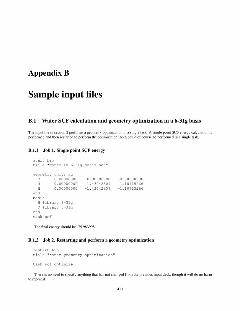
Appendix B
Sample input files
B.1 Water SCF calculation and geometry optimization in a 6-31g basis
The input file in section 2 performs a geometry optimization in a single task. A single point SCF energy calculation isperformed and then restarted to perform the optimization (both could of course be performed in a single task).
B.1.1 Job 1. Single point SCF energy
start h2otitle "Water in 6-31g basis set"
geometry units auO 0.00000000 0.00000000 0.00000000H 0.00000000 1.43042809 -1.10715266H 0.00000000 -1.43042809 -1.10715266
endbasis
H library 6-31gO library 6-31g
endtask scf
The final energy should be -75.983998.
B.1.2 Job 2. Restarting and perform a geometry optimization
restart h2otitle "Water geometry optimization"
task scf optimize
There is no need to specify anything that has not changed from the previous input deck, though it will do no harmto repeat it.
413

414 APPENDIX B. SAMPLE INPUT FILES
B.2 Compute the polarizability of Ne using finite field
B.2.1 Job 1. Compute the atomic energy
start netitle "Neon"geometry; ne 0 0 0; endbasis spherical
ne library aug-cc-pvdzendscf; thresh 1e-10; endtask scf
The final energy should be -128.496350.
B.2.2 Job 2. Compute the energy with applied field
An external field may be simulated with point charges. The charges here apply a field of magnitude 0.01 atomic unitsto the atom at the origin. Since the basis functions have not been reordered by the additional centers we can also restartfrom the previous vectors, which is the default for a restart job.
restart netitle "Neon in electric field"geometry units atomic
bq1 0 0 100 charge 50ne 0 0 0bq2 0 0 -100 charge -50
endtask scf
The final energy should be -128.496441, which together with the previous field-free result yields an estimate forthe polarizability of 1.83 atomic units. Note that by default NWChem does not include the interaction between thetwo point charges in the total energy (section 6).
B.3 SCF energy of H2CO using ECPs for C and O
The following will compute the SCF energy for formaldehyde with ECPs on the Carbon and Oxygen centers.
title "formaldehyde ECP deck"
start ecpchho
geometry units auC 0.000000 0.000000 -1.025176O 0.000000 0.000000 1.280289H 0.000000 1.767475 -2.045628H 0.000000 -1.767475 -2.045628

B.3. SCF ENERGY OF H2CO USING ECPS FOR C AND O 415
end
basisC SP0.1675097360D+02 -0.7812840500D-01 0.3088908800D-010.2888377460D+01 -0.3741108860D+00 0.2645728130D+000.6904575040D+00 0.1229059640D+01 0.8225024920D+00
C SP0.1813976910D+00 0.1000000000D+01 0.1000000000D+01
C D0.8000000000D+00 0.1000000000D+01
C F0.1000000000D+01 0.1000000000D+01
O SP0.1842936330D+02 -0.1218775590D+00 0.5975796600D-010.4047420810D+01 -0.1962142380D+00 0.3267825930D+000.1093836980D+01 0.1156987900D+01 0.7484058930D+00
O SP0.2906290230D+00 0.1000000000D+01 0.1000000000D+01
O D0.8000000000D+00 0.1000000000D+01
O F0.1100000000D+01 0.1000000000D+01
H S0.1873113696D+02 0.3349460434D-010.2825394365D+01 0.2347269535D+000.6401216923D+00 0.8137573262D+00
H S 1 1.000.1612777588D+00 0.1000000000D+01
end
ecpC nelec 2C ul
1 80.0000000 -1.600000001 30.0000000 -0.400000002 0.5498205 -0.03990210
C s0 0.7374760 0.638108320 135.2354832 11.009162302 8.5605569 20.13797020
C p2 10.6863587 -3.246842802 23.4979897 0.78505765
O nelec 2O ul
1 80.0000000 -1.600000001 30.0000000 -0.400000002 1.0953760 -0.06623814
O s0 0.9212952 0.39552179

416 APPENDIX B. SAMPLE INPUT FILES
0 28.6481971 2.516548432 9.3033500 17.04478500
O p2 52.3427019 27.977907702 30.7220233 -16.49630500
end
scfvectors input hcoremaxiter 20
end
task scf
This should produce the following output:
Final RHF results------------------
Total SCF energy = -22.507927218024One electron energy = -71.508730162974Two electron energy = 31.201960019808
Nuclear repulsion energy = 17.798842925142
B.4 MP2 optimization and CCSD(T) on nitrogen
The following performs an MP2 geometry optimization followed by a CCSD(T) energy evaluation at the convergedgeometry. A Dunning correlation-consistent triple-zeta basis is used. The default of Cartesian basis functions must beoverridden using the keyword spherical on the BASIS directive. The 1s core orbitals are frozen in both the MP2and coupled-cluster calculations (note that these must separately specified). The final MP2 energy is -109.383276, andthe CCSD(T) energy is -109.399662.
start n2
geometrysymmetry d2hn 0 0 0.542
end
basis sphericaln library cc-pvtz
end
mp2freeze core
end
task mp2 optimize

B.4. MP2 OPTIMIZATION AND CCSD(T) ON NITROGEN 417
ccsdfreeze core
end
task ccsd(t)

418 APPENDIX B. SAMPLE INPUT FILES
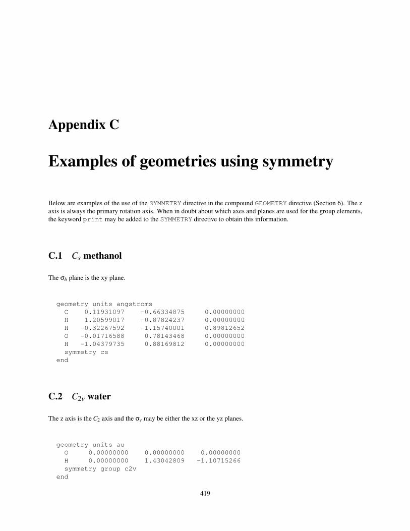
Appendix C
Examples of geometries using symmetry
Below are examples of the use of the SYMMETRY directive in the compound GEOMETRY directive (Section 6). The zaxis is always the primary rotation axis. When in doubt about which axes and planes are used for the group elements,the keyword print may be added to the SYMMETRY directive to obtain this information.
C.1 Cs methanol
The σh plane is the xy plane.
geometry units angstromsC 0.11931097 -0.66334875 0.00000000H 1.20599017 -0.87824237 0.00000000H -0.32267592 -1.15740001 0.89812652O -0.01716588 0.78143468 0.00000000H -1.04379735 0.88169812 0.00000000symmetry cs
end
C.2 C2v water
The z axis is the C2 axis and the σv may be either the xz or the yz planes.
geometry units auO 0.00000000 0.00000000 0.00000000H 0.00000000 1.43042809 -1.10715266symmetry group c2v
end
419

420 APPENDIX C. EXAMPLES OF GEOMETRIES USING SYMMETRY
C.3 D2h acetylene
Although acetylene has symmetry D∞h the subgroup D2h includes all operations that interchange equivalent atomswhich is what determines how much speedup you gain from using symmetry in building a Fock matrix.
The C2 axes are the x, y, and z axes. The σ planes are the xy, xz and yz planes. Generally, the unique atoms areplaced to use the z as the primary rotational axis and use the xz or yz planes as the σ plane.
geometry units ausymmetry group d2hC 0.000000000 0.000000000 -1.115108538H 0.000000000 0.000000000 -3.106737425
end
C.4 D2h ethylene
The C2 axes are the x, y, and z axes. The σ planes are the xy, xz and yz planes. Generally, the unique atoms are placedto use the z as the primary rotational axis and use the xz or yz planes as the σ plane.
geometry units angstromsC 0 0 0.659250H 0 0.916366 1.224352symmetry d2h
end
C.5 Td methane
For ease of use, the primary C3 axis should be the x=y=z axis. The 3 C2 axes are the x, y, and z.
geometry units auc 0.0000000 0.0000000 0.0000000h 1.1828637 1.1828637 1.1828637symmetry group Td
end
C.6 Ih buckminsterfullerene
One of the C5 axes is the z axis and the point of inversion is the origin.
geometry units angstroms # Bonds = 1.4445, 1.3945symmetry group Ihc -1.2287651 0.0 3.3143121
end

C.7. S4 PORPHYRIN 421
C.7 S4 porphyrin
The S4 and C2 rotation axis is the z axis. The reflection plane for the S4 operation is the xy plane.
geometry units angstromssymmetry group s4
fe 0.000 0.000 0.000h 2.242 6.496 -3.320h 1.542 4.304 -2.811c 1.947 6.284 -2.433c 1.568 4.987 -2.084h 2.252 8.213 -1.695c 1.993 7.278 -1.458h 5.474 -1.041 -1.143c 1.234 4.676 -0.765h 7.738 -1.714 -0.606c 0.857 3.276 -0.417h 1.380 -4.889 -0.413c 1.875 2.341 -0.234h 3.629 3.659 -0.234c 0.493 -2.964 -0.229c 1.551 -3.933 -0.221c 5.678 -1.273 -0.198c 1.656 6.974 -0.144c 3.261 2.696 -0.100n 1.702 0.990 -0.035
end
C.8 D3h iron penta-carbonyl
The C3 axis is the z axis. The σh plane is the xy plane. One of the perpendicular C2 axes is the x=y axis. One ofthe σv planes is the plane containing the x=y axis and the z axis. (The other axes and planes are generated by the C3operation.)
geometry units ausymmetry group d3h
fe 0.0 0.0 0.0
c 0.0 0.0 3.414358o 0.0 0.0 5.591323
c 2.4417087 2.4417087 0.0o 3.9810552 3.9810552 0.0
end

422 APPENDIX C. EXAMPLES OF GEOMETRIES USING SYMMETRY
C.9 D3d sodium crown ether
The C3 axis is the z axis. The point of inversion is the origin. One of the perpendicular C2 axes is the x=y axis. One ofthe σd planes is the plane containing the -x=y axis and the z axis.
Note that the oxygen atom is rotated in the x-y plane 15 degrees away from the y-axis so that it lies in a mirrorplane. There is a total of six atoms generated from the unique oxygen, in contrast to twelve from each of the carbonand hydrogen atoms.
geometry units ausymmetry D3d
NA .0000000000 .0000000000 .0000000000O 1.3384771885 4.9952647969 .1544089284H 6.7342048019 -0.6723850379 2.6581562148C 6.7599180056 -0.4844977035 .6136583870H 8.6497577017 0.0709194071 .0345361934
end
C.10 C3v ammonia
The C3 axis is the z axis. One of the σv planes is the plane containing the x=y axis and the z axis.
geometry units angstromsN 0 0 -0.055H 0.665 0.665 -0.481symmetry c3v
end
C.11 D6h benzene
The C6 axis is the z axis. The point of inversion is the origin. One of the 6 perpendicular C′2 axes is the x=y axis. (-x=yworks as a C′′2 axis.) The σh plane is the xy plane. The σd planes contain the C′′2 axis and the z axis. The σv planescontain the C′2 axis and the z axis.
geometry units auC 1.855 1.855 0H 3.289 3.289 0symmetry D6h
end
C.12 C3h BO3H3
The C3 axis is the z axis. The σh plane is the xy plane.

C.13. D5D FERROCENE 423
geometry units aub 0 0 0o 2.27238285 1.19464491 0.00000000h 2.10895420 2.97347707 0.00000000symmetry C3h
end
C.13 D5d ferrocene
The C5 axis is the z axis. The center of inversion is the origin. One of the perpendicular C2 axes is the x axis. One ofthe σd planes is the yz plane.
geometry units angstromssymmetry d5d
fe 0 0 0c 0 1.194 1.789h 0 2.256 1.789
end
C.14 C4v SF5Cl
The C4 axis is the z axis. The σv planes are the yz and the xz planes. The σd planes are: 1) the plane containing thex=y axis and the z axis and 2) the plane containing the -x=y axis and the z axis.
geometry units auS 0.00000000 0.00000000 -0.14917600Cl 0.00000000 0.00000000 4.03279700F 3.13694200 0.00000000 -0.15321800F 0.00000000 0.00000000 -3.27074500
symmetry C4vend
C.15 C2h trans-dichloroethylene
The C2 axis is the z axis. The origin is the inversion center. The σh plane is the xy plane.
geometry units angstromsC 0.65051239 -0.08305064 0Cl 1.75249381 1.30491767 0H 1.14820954 -1.04789741 0symmetry C2h
end

424 APPENDIX C. EXAMPLES OF GEOMETRIES USING SYMMETRY
C.16 D2d CH2CCH2
The C2 axis is the z axis (z is also the S4 axis). The x and y axes are the perpendicular C′2s. The σd planes are: 1) theplane containing the x=y axis and the z axis and 2) the plane containing the -x=y axis and the z axis.
geometry units angstromssymmetry d2dc 0 0 0c 0 0 1.300h 0.656 0.656 1.857
end
C.17 D5h cyclopentadiene anion
The C5 axis is the z axis (z is also the S5 axis). The y axis is one of the perpendicular C2 axes. The σh plane is the xyplane and one of the σd planes is the yz plane.
charge -1geometry units angstroms
symmetry d5hc 0 1.1853 0h 0 2.2654 0
end
C.18 D4h gold tetrachloride
The C4 axis is the z axis (z is also the S4 axis). The C′2 axes are the x and y axes and the C′′2 axes are the x=y axis andthe x=-y axis. The inversion center is the origin. The σh plane is the xy plane. The σv planes are the xz and yz planesand the σd planes are 1) the plane containing the x=-y axis and the z axis and 2) the plane containing the x=y axis andthe z axis.
geometry units auAu 0 0 0Cl 0 4.033 0symmetry D4h
end

Appendix D
Running NWChem
The command required to invoke NWChem is machine dependent, whereas most of the NWChem input is machineindependent1 .
D.1 Sequential execution
To run NWChem sequentially on nearly all UNIX-based platforms simply use the command nwchem and provide thename of the input file as an argument (See section 2.1 for more information). This does assume that either nwchem isin your path or you have set an alias of nwchem to point to the appropriate executable.
Output is to standard output, standard error and Fortran unit 6 (usually the same as standard output). Files arecreated by default in the current directory, though this may be overridden in the input (section 5.2).
Generally, one will run a job with the following command:
nwchem input.nw >& input.out &
D.2 Parallel execution on UNIX-based parallel machines including work-station clusters using TCGMSG
These platforms require the use of the TCGMSG2 parallel command and thus also require the definition of aprocess-group (or procgroup) file. The process-group file describes how many processes to start, what program to run,which machines to use, which directories to work in, and under which userid to run the processes. By convention theprocess-group file has a .p suffix.
The process-group file is read to end-of-file. The character # (hash or pound sign) is used to indicate a commentwhich continues to the next new-line character. Each line describes a cluster of processes and consists of the followingwhitespace separated fields:
userid hostname nslave executable workdir
1Machine dependence within the input arises from file names, machine specific resources, and differing services provided by the operatingsystem.
2Where required TCGMSG is automatically built with NWChem.
425

426 APPENDIX D. RUNNING NWCHEM
• userid – The user-name on the machine that will be executing the process.
• hostname – The hostname of the machine to execute this process. If it is the same machine on which parallelwas invoked the name must match the value returned by the command hostname. If a remote machine it mustallow remote execution from this machine (see man pages for rlogin, rsh).
• nslave – The total number of copies of this process to be executing on the specified machine. Only “clusters”of identical processes specified in this fashion can use shared memory to communicate. If no shared memory issupported on machine <hostname> then only the value one (1) is valid.
• executable – Full path name on the host <hostname> of the image to execute. If <hostname> is thelocal machine then a local path will suffice.
• workdir – Full path name on the host <hostname> of the directory to work in. Processes execute a chdir()to this directory before returning from pbegin(). If specified as a “.” then remote processes will use the logindirectory on that machine and local processes (relative to where parallel was invoked) will use the currentdirectory of parallel.
For example, if your file "nwchem.p" contained the following
d3g681 pc 4 /msrc/apps/bin/nwchem /scr22/rjh
then 4 processes running NWChem would be started on the machine pc running as user d3g681 in directory"/scr22/rjh". To actually run this simply type:
parallel nwchem big_molecule.nw
N.B. : The first process specified (process zero) is the only process that
• opens and reads the input file, and
• opens and reads/updates the database.
Thus, if your file systems are physically distributed (e.g., most workstation clusters) you must ensure that process zerocan correctly resolve the paths for the input and database files.
N.B. In releases of NWChem prior to 3.3 additional processes had to be created on workstation clusters to supportremote access to shared memory. This is no longer the case. The TCGMSG process group file now just needs to referto processes running NWChem.
D.3 Parallel execution on UNIX-based parallel machines including work-station clusters using MPI
To run with MPI, parallel should not be used. The way we usually run nwchem under MPI are the following
• using mpirun:
mpirun -np 8 $NWCHEM_TOP/bin/$NWCHEM_TARGET/nwchem input.nw
• If you have all nodes connected via shared memory and you have installed the ch_shmem version of MPICH,you can do
$NWCHEM_TOP/bin/$NWCHEM_TARGET/nwchem -np 8 h2o.nw

D.4. PARALLEL EXECUTION ON MPPS 427
D.4 Parallel execution on MPPs
All of these machines require use of different commands in order to gain exclusive access to computational resources.
D.5 IBM SP
If using POE (IBM’s Parallel Operating Environment) interactively, simply create the list of nodes to use in the file"host.list" in the current directory and invoke NWChem with
nwchem <input_file> -procs <n>
where n is the number of processes to use. Process 0 will run on the first node in "host.list" and must haveaccess to the input and other necessary files. Very significant performance gains may be had by setting the followingenvironment variables before running NWChem (or setting them using POE command line options).
• setenv MP_EUILIB us — dedicated user space communication over the switch (the default is IP over theswitch which is much slower).
• setenv MP_CSS_INTERRUPT yes — enable interrupts when a message arrives (the default is to pollwhich significantly slows down global array accesses).
In addition, if the IBM is running PSSP version 3.1, or later
• setenv MP_MSG_API lapi, or
• setenv MP_MSG_API mpi,lapi (if using both GA and MPI)
For batch execution, we recommend use of the llnw command which is installed in /usr/local/bin on theEMSL/PNNL IBM SP. If you are not running on that system, the llnw script may be found in the NWChem distribu-tion directory contrib/loadleveler. Interactive help may be obtained with the command llnw -help. Otherwise, thevery simplest job to run NWChem in batch using Load Leveller is something like this
#!/bin/csh -x# @ job_type = parallel# @ class = small# @ network.lapi = css0,not_shared,US# @ input = /dev/null# @ output = <OUTPUT_FILE_NAME># @ error = <ERROUT_FILE_NAME># @ environment = COPY_ALL; MP_PULSE=0; MP_SINGLE_THREAD=yes; MP_WAIT_MODE=yield; restart=no# @ min_processors = 7# @ max_processors = 7# @ cpu_limit = 1:00:00# @ wall_clock_limit = 1:00:00# @ queue#
cd /scratch
nwchem <INPUT_FILE_NAME>

428 APPENDIX D. RUNNING NWCHEM
Substitute <OUTPUT_FILE_NAME>, <ERROUT_FILE_NAME> and <INPUT_FILE_NAME> with the full pathof the appropriate files. Also, if you are using an SP with more than one processor per node, you will need to substitute
# @ network.lapi = css0,shared,US# @ node = NNODE# @ tasks_per_node = NTASK
for the lines
# @ network.lapi = css0,not_shared,US# @ min_processors = 7# @ max_processors = 7
where NNODE is the number of physical nodes to be used and NTASK is the number of tasks per node.
These files and the NWChem executable must be in a file system accessible to all processes. Put the above into afile (e.g., "test.job") and submit it with the command
llsubmit test.job
It will run a 7 processor, 1 hour job in the queue small. It should be apparent how to change these values.
Note that on many IBM SPs, including that at EMSL, the local scratch disks are wiped clean at the beginning ofeach job and therefore persistent files should be stored elsewhere. PIOFS is recommended for files larger than a fewMB.
D.6 Cray T3E
mpprun -n <npes> $NWCHEM_TOP/bin/$NWCHEM_TARGET/nwchem <input_file>
where npes is the number of processors and input_file is the name of your input file.
D.7 Alpha systems with Quadrics switch
prun -n <npes> $NWCHEM_TOP/bin/$NWCHEM_TARGET/nwchem <input_file>
where npes is the number of processors and input_file is the name of your input file.
D.8 Windows 98 and NT
$NWCHEM_TOP/bin/win32/nw32 <input_file>
where and input_file is the name of your input file. If you use WMPI, you must have a file named nw32.pgin the $NWCHEM_TOP/bin/win32 directory; the file must only contains the following single line
local 0

D.9. TESTED PLATFORMS AND O/S VERSIONS 429
D.9 Tested Platforms and O/S versions
• IBM SP with Power 3 and Power 4 nodes, AIX 5.1 and PSSP 3.4; IBM RS6000 workstation, AIX 5.1. Xlf8.1.0.0 and 8.1.0.1 are known to produce bad code.
• SGI R12000 IRIX 6.5
• SUN workstations with Solaris 2.6 and 2.8. Fujitsu SPARC systems (thanks to Herbert Früchtl) with Parallelnavicompilers.
• HP DEC alpha workstation , Tru64 V5.1, Compaq Fortran V5.3, V5.4.2, V5.5.1
• Linux with Intel x86 cpus. NWChem Release 4.5 has been tested on RedHat 6.x and 7.x, Mandrake 7.x. Wehave tested NWChem on Linux for the Power PC Macintosh with Yellow Dog 2.4. These all use the GCCcompiler at different levels. The Intel Fortran Compiler version 7 is supported. The Portland Group Compilerhas been tested in a less robust manner. Automatic generation of SSE2 optimized code is available when theIntel compiler is used (ifc vs g77 performances gain of 40% in some benchmarks) A somewhat Athlon optimizedcode can be generated under the GNU or Intel compilers by typing make _CPU=k7. GCC3 specific optionscan be turned on by typing make GCC31=y
• HP 9000/800 workstations with HPUX B.11.00. f90 must be used for compilation.
• Intel x86 with Windows 2000 has been tested with Compaq Visual Fortran 6.0 and 6.1 with WMPI 1.3 orNT-Mpich. NT-MPICH is available from http://www-unix.mcs.anl.gov/˜ashton/mpich.nt/
• Intel IA64 under Linux (with Intel compilers version 7 and later) and under HPUX.
• Fujitsu VPP computers.