AN INTRODUCTION TO MCSCF: PART 2

ORBITAL APPROXIMATION

•  Hartree product (hp) expressed as a product of spinorbitals ψι = φiσi

•  φi = space orbital, σi = spin function (α,β)•  Pauli Principle requires antisymmetry:

•  Closed Shells:

ORBITAL APPROXIMATION

•  For more complex species (one or more open shells) antisymmetric wavefunction is generally expressed as a linear combination of Slater determinants

•  For example, consider simple excited state represented by excitation φi->φa out of closed shell:

•  For more complex open shell species (e.g., low-spin open shells with multiple partially filled orbitals, such as s1d7 Fe) wavefunctions are linear combinations of several determinants.

•  But, the coefficients on these determinants are determined by spin and symmetry, not by the Variational Principle

HARTREE-FOCK METHOD •  Optimization of the orbitals (minimization of

the energy with respect to all orbitals), based on the Variational Principle) leads to Hartree-Fock equations (closed shells):

•  For open shells, there are multiple Fock operators, one for each type of orbital occupancy; e.g. UHF:

LCAO METHOD

•  Generally solve HF problem by LCAO expansion: expand φi as linear combination of basis functions (AOs), χµ:

•  The Cµi are expansion coefficients obtained via the Variational Principle –  FC = SCε –  HFR matrix equation, solved iteratively

MCSCF METHOD

•  Hartree-Fock (or DFT) is most common zeroth order wavefunction, but

•  Many problems are not well represented by single configuration wavefunctions: –  Diradicals (broadly defined) –  Excited states –  Transition states (frequently) –  Unsaturated transition metals –  High energy species –  Generally, any system with near degeneracies

•  In such cases, the correct zeroth order wavefunction is MCSCF:

•  Φ is the MCSCF wavefunction •  ΨK is a configuration wavefunction

– Can be a single determinant – Could be a linear combination of

determinants in order to be spin-correct – Generally called configuration state function

(CSF), meaning spin-correct, symmetry- correct configuration wavefunction

•  Generally, two approaches to treating Φ in computer codes: –  Expand in terms of CSFs

•  Most commonly GUGA (graphical unitary group approach)

•  Made feasible by Shavitt, Schaefer –  Expand directly in terms of determinants

•  Can be faster code •  More determinants to deal with •  Each determinant not spin-correct, but easily dealt with •  Not as robust: GUGA code is generally preferred •  Some applications only available for determinant code

– Both available in GAMESS

•  AK are CI expansion coefficients –  Determined variationally using linear variation

theory

•  Solution of this (non-iterative) matrix eigenvalue equation yields –  MCSCF energies EM for each electronic state –  CI coefficients AKM corresponding to state M

MCSCF METHOD

•  Solution of MCSCF problem requires two sets of iterations to solve for two sets of coefficients –  For each set of CI coefficients AK, solve for LCAO

coefficients Cµi (micro-iterations) –  For given set of Cµi, solve CI equations for new

AK

– Continue until self-consistency

MCSCF METHOD

•  Most common implementation is FORS (fully optimized reaction space)/CASSCF (complete active space) SCF – Define active space in terms of orbitals and

electrons – Perform full CI within active space – Very “chemical” approach – Can be computationally demanding

•  Ideal active space is full valence •  Not always feasible; upper limit is ~(16,16)

– Sometimes tricky to choose active space

•  Two sets of coefficient optimizations – CI coefficients optimized by solving linear

variation secular equation – Orbital optimization analogous to, but

more complex than, simple HF solutions •  Need to optimize mixing between sets of

subspaces:core, active, virtual – Core-active –  Active-virtual – Core-virtual

•  Cf., HF high-spin open shell: Fock operators for

– Doubly occupied-singly occupied – Doubly occupied-virtual –  Singly occupied virtual

•  Orbital optimizations – As for HF, each subspace invariant to

internal mixing – Only mixing between subspaces will change

energy –  Exception: if MCSCF is not FORS/

CASSCF (CI is not Full CI), must also optimize active-active mixing: •  FORS simpler although more demanding

computationally •  Non-FORS less robust, more difficult to

converge – Can think of optimization variables as

rotation angles connecting orbitals in different subspaces (recall UHF)

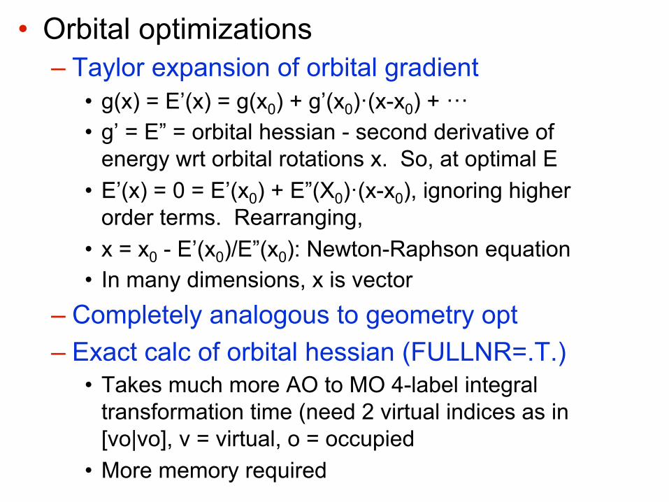
•  Orbital optimizations – Taylor expansion of orbital gradient

•  g(x) = E’(x) = g(x0) + g’(x0)·(x-x0) + ··· •  g’ = E” = orbital hessian - second derivative of

energy wrt orbital rotations x. So, at optimal E •  E’(x) = 0 = E’(x0) + E”(X0)·(x-x0), ignoring higher

order terms. Rearranging, •  x = x0 - E’(x0)/E”(x0): Newton-Raphson equation •  In many dimensions, x is vector

– Completely analogous to geometry opt – Exact calc of orbital hessian (FULLNR=.T.)

•  Takes much more AO to MO 4-label integral transformation time (need 2 virtual indices as in [vo|vo], v = virtual, o = occupied

•  More memory required

– As in geom opt, alternative to FULLNR is approximate updating of orbital hessian

•  SOSCF=.T.: calc diagonal, guess off-diagonal •  Takes more iterations, but less time. •  Convergence less robust •  Easily can do 750 basis functions on workstation

– Alternatives are •  JACOBI: simple pairwise rotations, similar to

SCFDM •  FOCAS: uses only orbital gradients, not even

diagonal hessian elements as in SOSCF. Each iteration is faster, but many more required

– Best strategy •  Start with SOSCF •  Use FULLNR as backup

CHOOSING ACTIVE SPACES

•  Full valence active space – Occupied orbitals are usually easy: choose

all of them. – Virtual orbitals not always easy:

•  # of orbitals wanted = minimal valence basis set •  # of available virtuals generally much larger •  Virtuals are generally more diffuse and not easy

to identify, especially with –  Large basis sets, especially diffuse functions –  Transition metals – High symmetry

•  Strategies for full valence active space – MVOQ in $SCF

•  Since virtual MOs are typically diffuse, ease of identification is improved if they are made more compact

•  MVOQ = n removes n electrons from SCF calculation •  Generates a cation with +n charge - pulls orbitals in •  Easier to find correct virtuals for active space •  Improved convergence

•  Strategies for full valence active space – Localized orbitals (LMOs)

•  Specify LOCAL=BOYS or RUDNBERG in $CONTRL •  Transforms orbitals to bonds, lone pairs •  Easier to understand occupied FV space •  Can use these to construct virtual part of FV active

space •  Disadvantage: LMOs destroy symmetry, so the size of

the problem (# of determinants) increases •  Partial solution: symmetry localized orbitals can be

specified using SYMLOC=.T. in $LOCAL –  Localizes orbitals only within each irrep –  Sometimes not localized enough

•  Strategies for less than FV active space – Need to identify “chemically important” orbitals

•  Orbitals directly involved in the chemical process •  Orbitals that may interact strongly with reacting orbitals

– Examples •  Recall H2:

–  Active space includes H-H bonding orbital and H-H* –  FORS(2,2): 2 electrons in 2 orbitals

•  Internal rotation in ethylene – Full Valence active space is (12,12) – Minimum active space includes only CC σ,π,π∗,σ∗: (4,4) –  The two active spaces give ~same internal rotation barrier –  This active space cannot account for other processes, such as

C-H bond cleavage

– More Examples •  Internal rotation in H2C=NH

– Start with analogous active space to ethylene: CN (4,4) – Recognize that N lone pair will interact with π system as

internal rotation takes place – Add N lone pair to active space: (6,5), 6 electrons in 5 orbitals – Also correctly describes dissociation to H2C + NH: NH

fragment will be correctly described by σ2πx1πy

1

•  Dissociation of H2C=O -> H2C + O –  Again, start with CO (4,4) – Recognize O has two lone pairs, one 2s, one 2p – Recognize that 2s lone pair has low energy & likely inactive –  Including 2p lone pair [(6,5) active space] ensures three 2p

orbitals are treated equally in dissociated oxygen –  Isomerization to HCOH requires additional (4,4) from CH/OH

•  Important to consider both reactant and product when choosing active space – Ensures number of active electrons & orbitals are

same – Verifies reactant orbitals will be able to convert

smoothly into product orbitals. – Transition state orbitals can help make this

transition smooth

– Consider isomerization of bicyclobutane to 1,3-butadiene

•  Superficially only need to break two bonds: FORS(4,4) •  But, to treat all peripheral bonds equally, need all of

them in active space: FORS(10,10) –  Now, consider isoelectronic NO dimer, N2O2

•  Replace two bridge CH groups with nitrogens •  Replace two peripheral CH2 groups with oxygens •  Very high energy species: important HEDM compound •  First guess at good active space might be (10,10) •  But, one O lone pair on each O interacts strongly and

must be included in active space for smooth PES •  Correct active space is (14,12) •  Pay attention to orbitals along reaction path!

MULTI-REFERENCE DYNAMIC CORRELATION

•  Multi-reference CI: MRCI – CI from set of MCSCF configurations – Most commonly stops at singles and doubles

•  MR(SD)CI: Very demanding •  ~ very difficult to go past 16 electrons in 16 orbitals

•  Multi-reference perturbation theory – Several flavors: CASPT2, MRMP2, GVVPT2 – Mostly second order (except CASPT3) – More efficient than MRCI – Not usually as accurate as MRCI – Can “blow up” if perturbation is too big

MULTI-REFERENCE DYNAMIC CORRELATION

•  MRCI, MRPT generally not size-consistent – +Q correction can make MRCI nearly size

consistent – MRPT developers like to say the method is

“nearly size-consistent” Not really true

– Cf., GN methods are “slightly empirical”

STRATEGIES FOR INCONSISTENT ACTIVE SPACES

•  Sometimes different parts of PES require different active spaces. Strategies – Optimize geometries, obtain frequencies with

separate active spaces – Final MRPT or MRCI with composite active

space –  If composite active space is too large

•  Optimize geometries with separate active spaces •  Use MRPT with separate active spaces to correlate

all electrons

NATURAL ORBITAL ANALYSIS •  Complex wavefunctions like MCSCF are very

useful, but qualitative interpretations are important

•  Two useful tools are – Natural orbitals – Localized orbitals

•  Natural orbitals introduced by Löwdin in 1955 –  Diagonalize the 1st order density matrix ρ– Simply the HF orbitals for HF theory

NATURAL ORBITAL ANALYSIS

–  For fully variational methods (HF, MCSCF), 1st order density matrix is simply obtained from ΨΨ∗

–  For other methods (MPn, CC, MRMP), must also calculate non-Hellmann-Feynman contribution: requires gradient of energy

–  Eigenvectors of 1st order density matrix are natural orbitals

–  Eigenvalues are natural orbital occupation numbers (NOON): λi

NATURAL ORBITAL ANALYSIS – For RHF & ROHF, NOON are integers: 2,1,0 – For other methods,NOON are not integers

•  Deviation from 2 (occupied orbitals) or 0 (virtual orbitals) indicate importance of configurational mixing

•  For H2, λ1~2, λ2∼0 near Re; λ1, λ2 ∼1 near dissociation – NOON are also good diagnostic for need for

MCSCF zeroth order wavefunction •  NOON for single reference assume non-physical values

when such methods start to break down. – Examples

MCSCF/LMO/CI METHOD •  See Gordon&Cundari, Coord Chem Rev.,

147, 87-115 (1996) – Choose active space for particular bond type – Determine MCSCF LMOs within active space

•  These are atom-like in nature – Perform CI within LMO MCSCF space – Applied to analyze TM-MG double bonds

•  TM=transition metal (or Tom) •  MG=main group (or Mark Gordon)

•  Possible resonance contributors

–  Straight line = covalent structure, electrons shared –  Arrow = ionic structure, both electrons on atom at

base of arrow –  Lower arrow = σ, upper arrow = π

Table 1. Percent contributors of covalent and ionic resonancestructures in H2M=EH2 compounds. Nucleophilic structures aredefined as those with M+E- ionicity, electrophilic means M-E+

--- Ti --- --- Zr --- --- Nb --- --- Ta --- Si C Si C Si C Si C A 44.6 36.5 40.0 32.8 41.5 37.4 39.7 34.1 B 3.8 2.6 4.7 2.9 7.6 4.5 6.5 3.9

C 1.9 9.7 5.5 14.1 4.8 11.7 6.3 13.4

D 34.6 36.2 31.5 30.9 24.1 26.3 26.5 28.2

E 8.2 7.3 8.6 6.8 13.2 8.1 11.0 7.6

F 0.3 2.6 1.6 6.3 0.9 3.7 1.5 5.5

G 5.4 2.6 5.7 3.1 5.3 4.4 5.5 3.7

H 0.2 0.1 0.4 0.1 0.5 0.2 0.5 0.2

I 0.8 2.3 2.0 3.1 1.9 3.5 2.3 3.3

Neut. 53.6 46.1 50.6 42.7 56.0 49.0 53.0 45.0

Nucl. 36.8 48.5 38.6 51.4 29.8 41.7 35.3 47.1

Elec. 9.4 5.3 10.8 6.1 13.4 9.1 12.5 7.8

–  This method 1st to show σ ylide structure D is an important resonance contributor

STEPS TO RUN CASSCF •  RUN HF TO GET STARTING ORBITALS

– Grab $vec group from .dat & insert in input file •  Set up MCSCF input file

H2 INPUT FILE $CONTRL SCFTYP=MCSCF RUNTYP=ENERGY MULT=1 $END $BASIS GBASIS=N31 NGAUSS=6 NDFUNC=1 $END $GUESS GUESS=MOREAD NORB=4 $END $DATARHF/6-31G(d) H2DNH 2

HYDROGEN 1.0 .0000000000 .0000000000 .3650000000 $END--- CLOSED SHELL ORBITALS --- GENERATED AT Mon Aug 25 10:56:56 2008RHF/6-31G(d) H2E(RHF)= -1.1268278242, E(NUC)= 0.7249003414, 7 ITERS $VEC 1 1 3.28562555E-01 2.69295789E-01 3.28562555E-01 2.69295789E-01 2 1 1.20677971E-01 1.74055284E+00-1.20677971E-01-1.74055284E+00 3 1 7.61861020E-01-6.85623406E-01 7.61861020E-01-6.85623406E-01 4 1-1.13103226E+00 1.35731210E+00 1.13103226E+00-1.35731210E+00 $END $DRT NMCC=0 NDOC=1 NVAL=1 FORS=.T. GROUP=D2H $END $MCSCF CISTEP=GUGA FORS=.T. $END

H2 LOG FILE

$CONTRL SCFTYP=MCSCF RUNTYP=ENERGY NZVAR=3 COORD=ZMT $END $SYSTEM TIMLIM=5 MEMORY=300000 $END $BASIS GBASIS=STO NGAUSS=3 $END $DATA Methylene...1-A-1 state...MCSCF/STO-3G Cnv 2 C H 1 rCH H 1 rCH 2 aHOH rCH=1.09 aHOH=130.0 $END $GUESS GUESS=MOREAD NORB=7 $END $MCSCF CISTEP=GUGA $END $DRT NMCC=3 NDOC=1 NVAL=1 FORS=.T. GROUP=C2V $END --- RHF ORBITALS --- GENERATED AT 21:48:01 10-13-1999 Methylene...1-A-1 state...MCSCF/STO-2G E(RHF)= -38.3704886597, E(NUC)= 6.1450312399, 8 ITERS $VEC 1 1 9.93050334E-01 3.06416919E-02 0.00000000E+00 0.00000000E+00 7.13949414E-03 1 2-7.56284556E-03-7.56284556E-03 2 1-2.13664212E-01 6.49200772E-01 0.00000000E+00 0.00000000E+00 1.82338446E-01 2 2 2.71289288E-01 2.71289288E-01 3 1 0.00000000E+00 0.00000000E+00 5.42052798E-01 0.00000000E+00 0.00000000E+00 3 2-4.66619722E-01 4.66619722E-01 4 1 1.43219334E-01-6.53818237E-01 0.00000000E+00 0.00000000E+00 7.44709913E-01 4 2 2.24175347E-01 2.24175347E-01 5 1 0.00000000E+00 0.00000000E+00 0.00000000E+00 1.00000000E+00 0.00000000E+00 5 2 0.00000000E+00 0.00000000E+00 6 1 0.00000000E+00 0.00000000E+00 1.08196576E+00 0.00000000E+00 0.00000000E+00 6 2 8.37855220E-01-8.37855220E-01 7 1-1.69243066E-01 1.08779602E+00 0.00000000E+00 0.00000000E+00 8.71412547E-01 7 2-9.04841898E-01-9.04841898E-01 $END

! EXAM06. ! 1-A-1 CH2 MCSCF methylene geometry optimization. ! ! At the initial geometry: ! The initial energy is -37.187342653, ! the FINAL E= -37.2562020559 after 14 iterations, ! the RMS gradient is 0.0256396. ! ! After 4 steps, ! FINAL E= -37.2581791686, RMS gradient=0.0000013, ! r(CH)=1.1243359, ang(HCH)=98.8171674 ! $CONTRL SCFTYP=MCSCF RUNTYP=OPTIMIZE NZVAR=3 COORD=ZMT $END $SYSTEM TIMLIM=5 MEMORY=300000 $END $BASIS GBASIS=STO NGAUSS=2 $END $DATA Methylene...1-A-1 state...MCSCF/STO-2G Cnv 2 C H 1 rCH H 1 rCH 2 aHOH rCH=1.09 aHOH=99.0 $END $ZMAT ZMAT(1)=1,1,2, 1,1,3, 2,2,1,3 $END ! ! Normally one starts a MCSCF run with converged SCF orbitals $GUESS GUESS=HUCKEL $END ! ! two active electrons in two active orbitals. ! must find at least two roots since ground state is 3-B-1 ! $DET NCORE=3 NACT=2 NELS=2 NSTATE=2 $END

“ALTERNATIVES” TO MCSCF •  SINGLE REFERENCE METHODS

– Spin-Flip: Anna Krylov – Completely renormalized CCSD(T): Piecuch

•  Adds a denominator to CCSD(T) that permits correct single bond breaking

•  Potentially huge impact: Treats diradicals correctly •  Open or closed shells •  CCTYP=CR-CCL in GAMESS

RECENT DEVELOPMENTS •  ORMAS (Joe Ivanic)

– Occupation restricted multiple active spaces – Method for expanding size of MCSCF

•  Identify several smaller subspaces •  Also ORMAS-PT2

•  Eliminating deadwood from MCSCF, CI – Ruedenberg, Ivanic, Bytautas – Extrapolate to complete basis set –  Interpolate to exact Full CI – Allows full CI on much larger systems

•  Parallel MCSCF, CI