NWC Distinguished Lecture

Blind-source signal decomposition according to a general mathematical model

Charles K. Chui*

Hong Kong Baptist university and Stanford University

Norbert Wiener Center, UMD February 16, 2017

*Research supported by ARO Grant # W911NF-15-1-0385

Contents of presentation

1. Need of scientific models

2. From ARMA to exponential sums and damped sinusoids, and to a more general signal model (GSM)

3. Is this GSM natural and useful for real-world signal representation?

4. Time-scale-frequency approach: Synchrosqueezing transform (SST)

5. A direct time-frequency approach: Phase-preserving sub-signal separation operation (or operators) (PSSO)

6. Remarks and discussions

2

I. Need of scientific models

3

Can we find the “truth” by just “thinking” without using any scientific models?

Who am I? Where did I come from? Where will I be in afterlife?

Thinking man in deep thoughts

4

Origin of the universe and what next?Model for extrapolation in time

(13.8 billion years ago and some 40 billion years from now)

Big Bang theory and prediction models

5

Origins of life

Darwin’s “Evolution Theory: Ape and human chromosomes are 98% identical.” This has been proven incorrect.

In addition, humans have 23 pairs of chromosomes, while apes have 24 pairs. In fact, all primates, including: apes, gorillas, chimpanzees, and orangutans, have more chromosome pairs than humans. Dogs have 39 pairs.

If humans lose a pair of chromosomes, they cannot reproduce!

Although life’s beginnings on earth billions of years ago, “homo sapiens” discovered in Ethiopia were believed to be the oldest 'modern' human beings, and lived only 160,000 years ago.

6

Every real-world problem requires a justifiable model

Returning to earthly problems, consider the linear model

for seismic survey

7

Sound signals are used as impulse input with (unit) impulse response output

to locate oil traps

8

The main objective is to locate structural traps

Two types of oil & gas traps

9

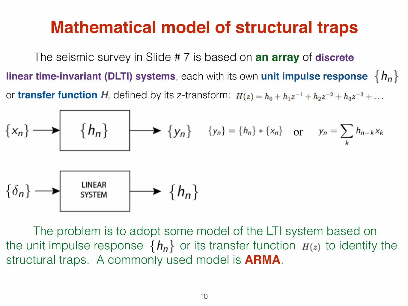
Mathematical model of structural traps The seismic survey in Slide # 7 is based on an array of discrete

linear time-invariant (DLTI) systems, each with its own unit impulse response

or transfer function H, defined by its z-transform:

The problem is to adopt some model of the LTI system based on the unit impulse response or its transfer function to identify the structural traps. A commonly used model is ARMA.

10

or

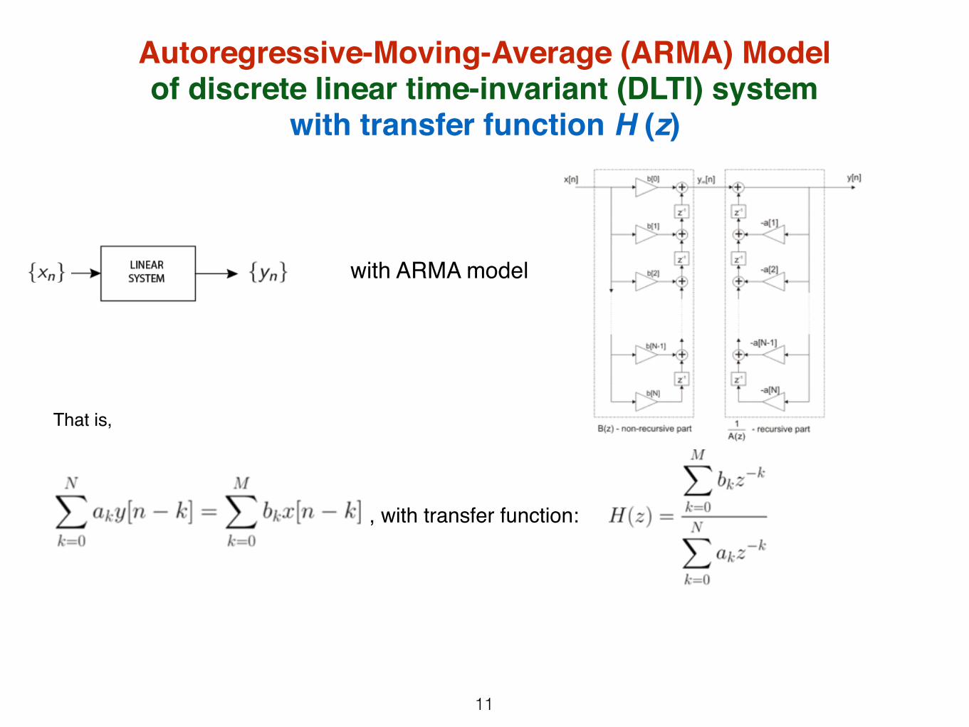
Autoregressive-Moving-Average (ARMA) Modelof discrete linear time-invariant (DLTI) system

with transfer function H (z)

with ARMA model

That is,

, with transfer function:

11

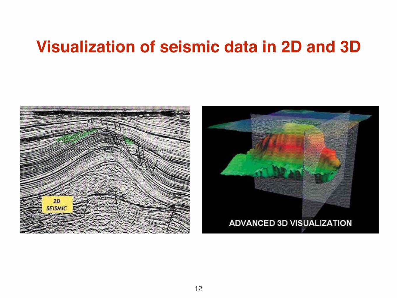
Visualization of seismic data in 2D and 3D

12

2. From ARMA to

Exponential sums and Damped sinusoids,and to

a more general signal model (GSM)

13

Continuous linear time-invariant (CLTI) System

We next consider continuous LTI systems h(t), with continuous-time input signal x(t) and output y(t). The transfer function H(s) of this system is now the Laplace transform of h(t)

14

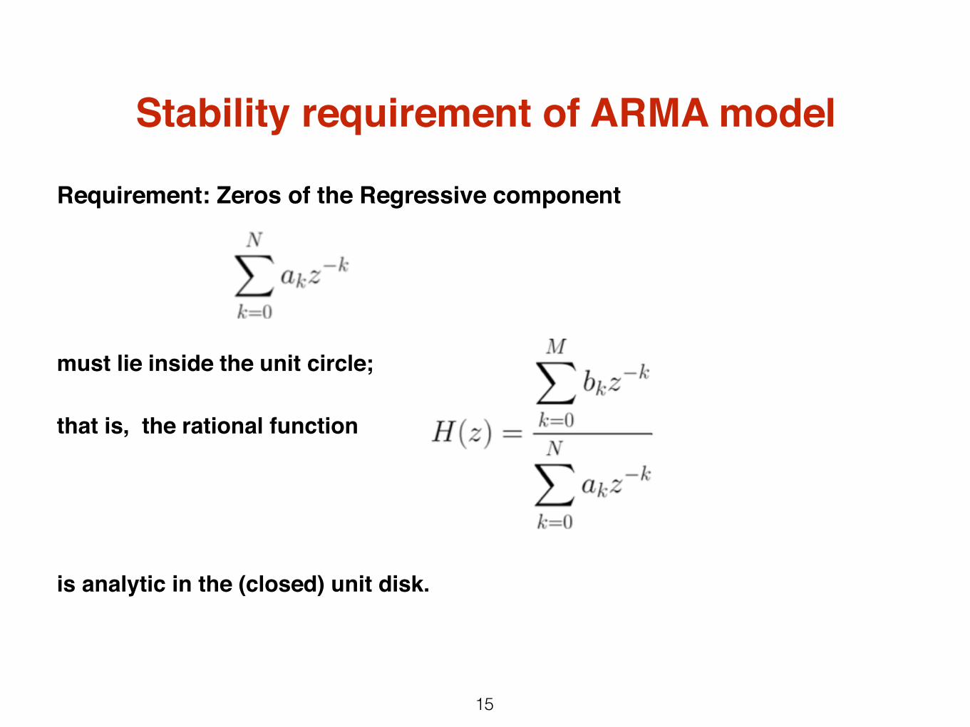
Stability requirement of ARMA model

Requirement: Zeros of the Regressive component

must lie inside the unit circle;

that is, the rational function

is analytic in the (closed) unit disk.

15

Stability requirement of CLTI systems

For convenience, we consider the model with transfer function, given by

16

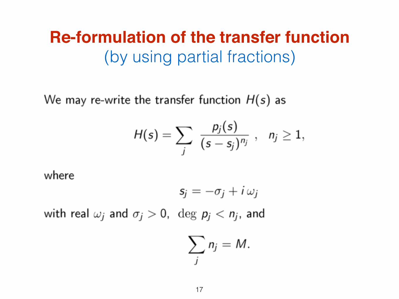
Re-formulation of the transfer function(by using partial fractions)

17

From time-domain formulationto

Exponential sums

(1)

18

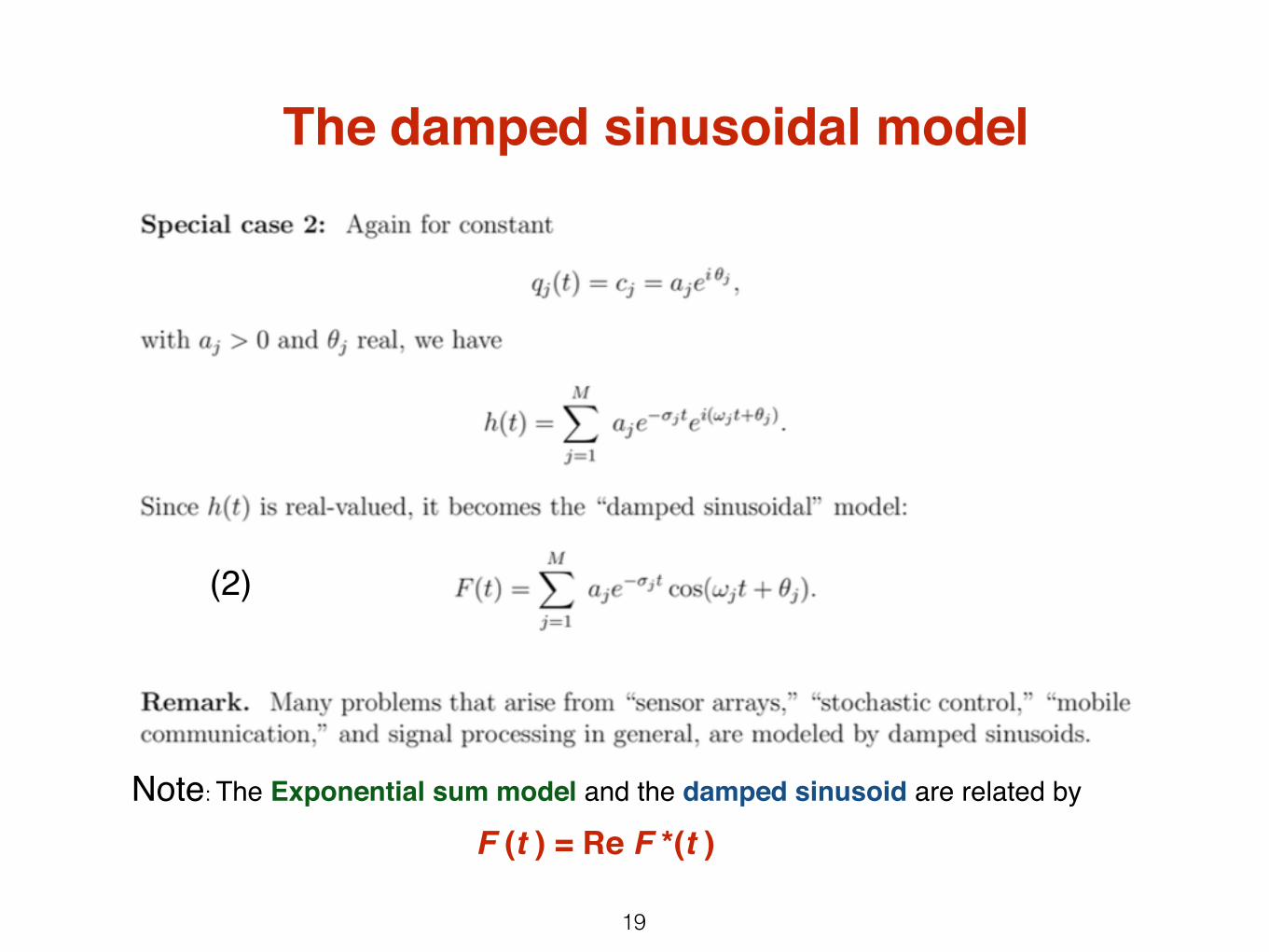
The damped sinusoidal model

19

Note: The Exponential sum model and the damped sinusoid are related by F (t ) = Re F *(t )

(2)

Early development in system identification of

LTI dynamic systems

In 1795, Gaspard de Prony (1755 -1839), a French Mathematician and Engineer, introduced a clever algorithm (called “Prony's method”) to fit an exponential sum model, for estimating the parameters of an LTI system, by using 2M evenly spaced samples h (k) = F *(k) (that is, the output with delta distribution at t = k input):

for k = 1, … , N, with N = 2M - 1. In other words, de Prony initiated the more general

where M is unknown, by choosing sufficiently large N > 2M - 2.

20

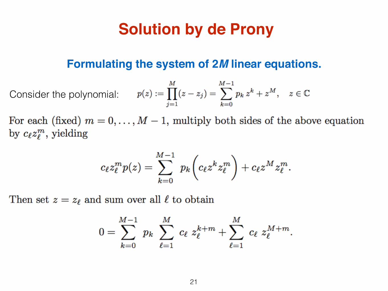
Solution by de Prony

Formulating the system of 2M linear equations.

Consider the polynomial:

21

The system of 2M linear equationsSince

for k = 0, . . . 2M -1, we have

By introducing the Hankel matrix

the above system of linear equations has the following matrix formulation:

22

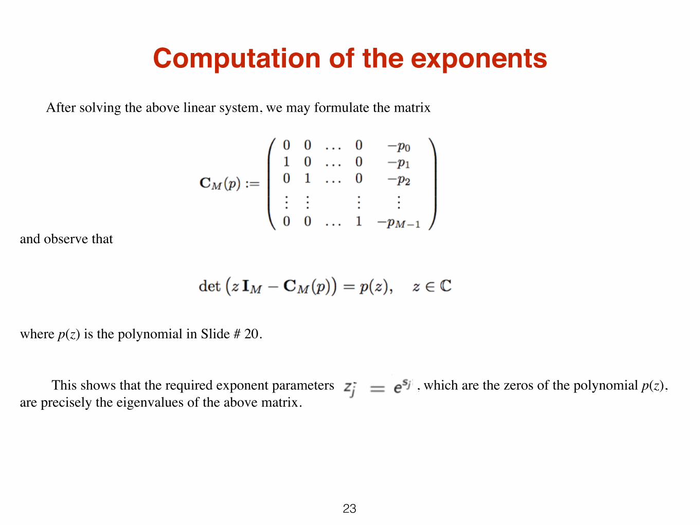
Computation of the exponents After solving the above linear system, we may formulate the matrix

and observe that

where p(z) is the polynomial in Slide # 20.

This shows that the required exponent parameters , which are the zeros of the polynomial p(z), are precisely the eigenvalues of the above matrix.

23

Computation of the coefficients

From the formulation of Prony’s problem in Slide # 20, the coefficients of the exponential sum

24

A more general signal model (GSM)

25

3. Is this GSM natural and useful for real-world signal representation?

26

Extension to analytic signals from Hilbert to Hardy-Littlewood and to Gabor

The Hilbert transform of a real-valued function f (on the real line or a bounded interval) is given, respectively, by:

In view of the development by Hardy (of Hardy spaces) and Littlewood (of the boundary value problem), the notion of “complex signal extension”

introduced in the pioneering paper, “Theory of Communication”, published in 1946 by J. IEE, by the Nobel Laureate Dennis Gabor using the Hilbert transform, can be called “analytic extension”, since the extended function is analytic in the upper half complex plane.

Taking the real part of the polar formulation of the analytic extension yields:

with

27

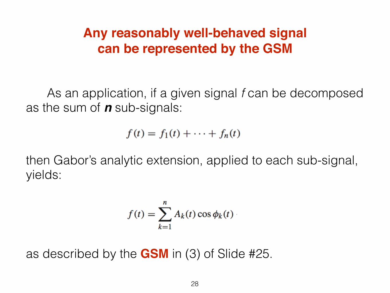
Any reasonably well-behaved signal can be represented by the GSM

As an application, if a given signal f can be decomposed as the sum of n sub-signals:

then Gabor’s analytic extension, applied to each sub-signal, yields:

as described by the GSM in (3) of Slide #25.

28

Challenges in decomposition of real-world signals

• Are there acceptable decomposition methods and effective computational schemes that could be applied to separate real-world signals into sub-signals?

• As in the consideration of damped sinusoids or exponential sums, it was already a challenge to determine the exact number M of sub-signals when some of the exponents are very close to one other.

• Prony’s method and its more recent modifications and generalizations often fail, particularly in the presence of additive noise.

29

Example: Empirical mode decomposition (EMD) is a popular computational scheme

introduced by N. Huang along with 8 co-authors published in the 1998 Proc. London Royal Society

EMD consists of two stages:

• The sifting process is applied to decompose the given signal f(t) as a finite sum of, say K, “Intrinsic mode functions” (IMF’s) and a remainder, R(t), which is an “almost” monotone function, with no noticeable oscillations.

• Extension of each sub-signal to an analytic signal via the Hilbert transform, followed by taking the real part of the polar representation of the extension, to meet the GSM signal format (3), as introduced in Slide # 24, namely:

30

The sifting process to decompose the given signal into sub-signals, called intrinsic mode functions (IMF’s)

Sifting process (see top image on right)

• Apply cubic spline interpolation to the local maxima of the data function to yield an upper envelope

• Apply cubic spline interpolation to the local minima of the data function to yield a lower envelope

• Compute the mean of the upper and lower envelopes • Subtract this mean from the data function • Repeat the above procedure to the difference of the

data function and the mean • Iterate the same procedure till the mean of the upper

and lower envelopes is near “0”

Intrinsic mode functions, IMF’s (see 6 IMF’s in bottom image)

• The difference of the given data function and the (first) sum of the means obtained from the sifting process is called the first IMF C_1

• Consider the sum of the means as a new “data function” and apply the sifting process to obtain the “second sum” of means. The second IMF C_2 is the difference of the first and second sums of the means

• Repeat the same procedure till the sum of means does not have any local extrema; i.e. is monotonic increasing or decreasing

• The monotone residue function may be considered as the “trend” of the the data function

31

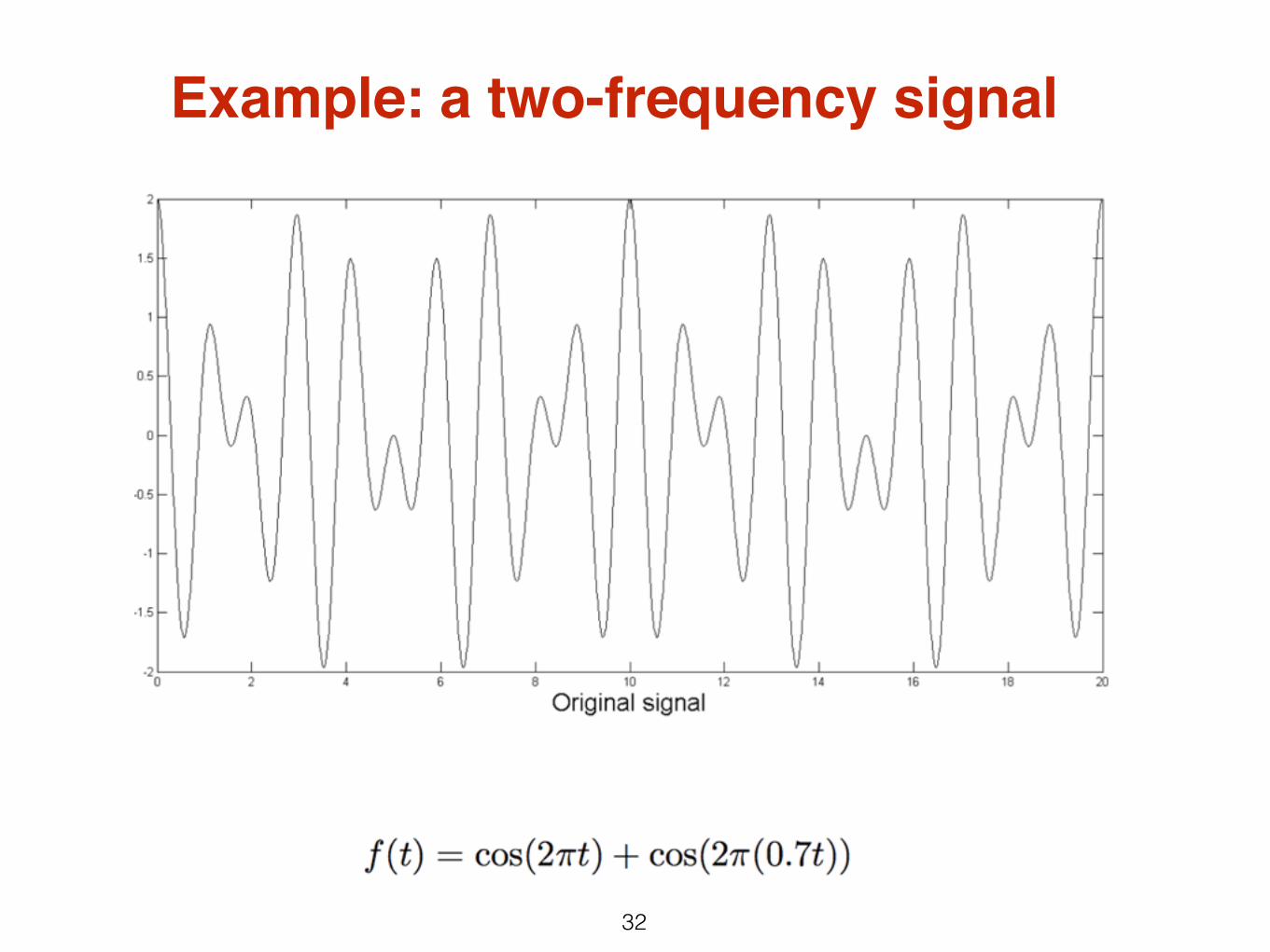
Example: a two-frequency signal

32

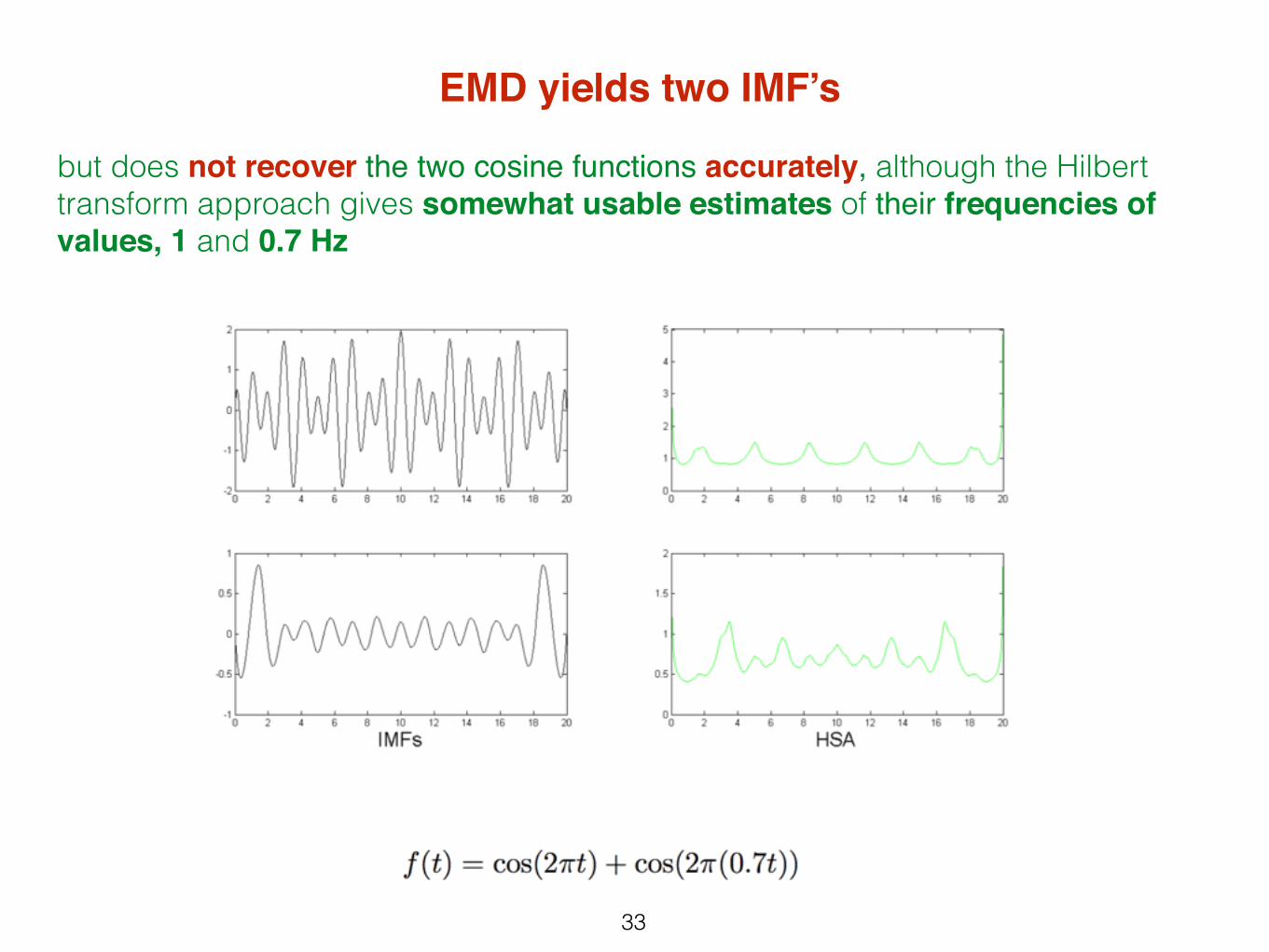
EMD yields two IMF’s

but does not recover the two cosine functions accurately, although the Hilbert transform approach gives somewhat usable estimates of their frequencies of values, 1 and 0.7 Hz

33

Model specifications required for theoretical development

Although the EMD scheme decomposes “any” blind-source signal according to the GSM format, the performance is poor, even for the above toy example of the sum of two cosines with well separated frequencies.

34

Adaptive harmonic model

35

4. Time-scale-frequency approach:

Synchrosqueezing transform, (SST)

based on the AHM, with certain restrictive specifications

36

Synchrosqueezing transform (SST) This innovative approach is to introduce an “instantaneous frequency information function” (IFIF) of two variables, in time and scale, and then to squeeze out all the instantaneous frequencies (IF’s) of all “possible sub-signals” at the same (fixed) time instant b, for each chosen b. For this approach to work, certain restrictive technical specifications are imposed on the AHM.

First introduced, in:

Then rigorously developed, in:

Samples of more recent development:

H. Yang, Synchrosqueezed wave packet transforms and diffeomorphism-based spectral analysis for 1D general mode decompositions, Applied and Computational Harmonic Analysis, Vol. 39(1) (2015), 33-66.

J. Xu, H. Yang, and I. Daubechies, Recursive diffeomorphism-based regression for shape functions. arXiv:1610.03819, submitted to SIAM J. on Math Anal.

B. Cornelis, H. Yang, A. Goodfriend, N. Ocon, J. Lu, and I. Daubechies, Removal of canvas patterns in digital acquisitions of painting. IEEE Trans. Image Proc. 26(1)(2017), 160-171.

37

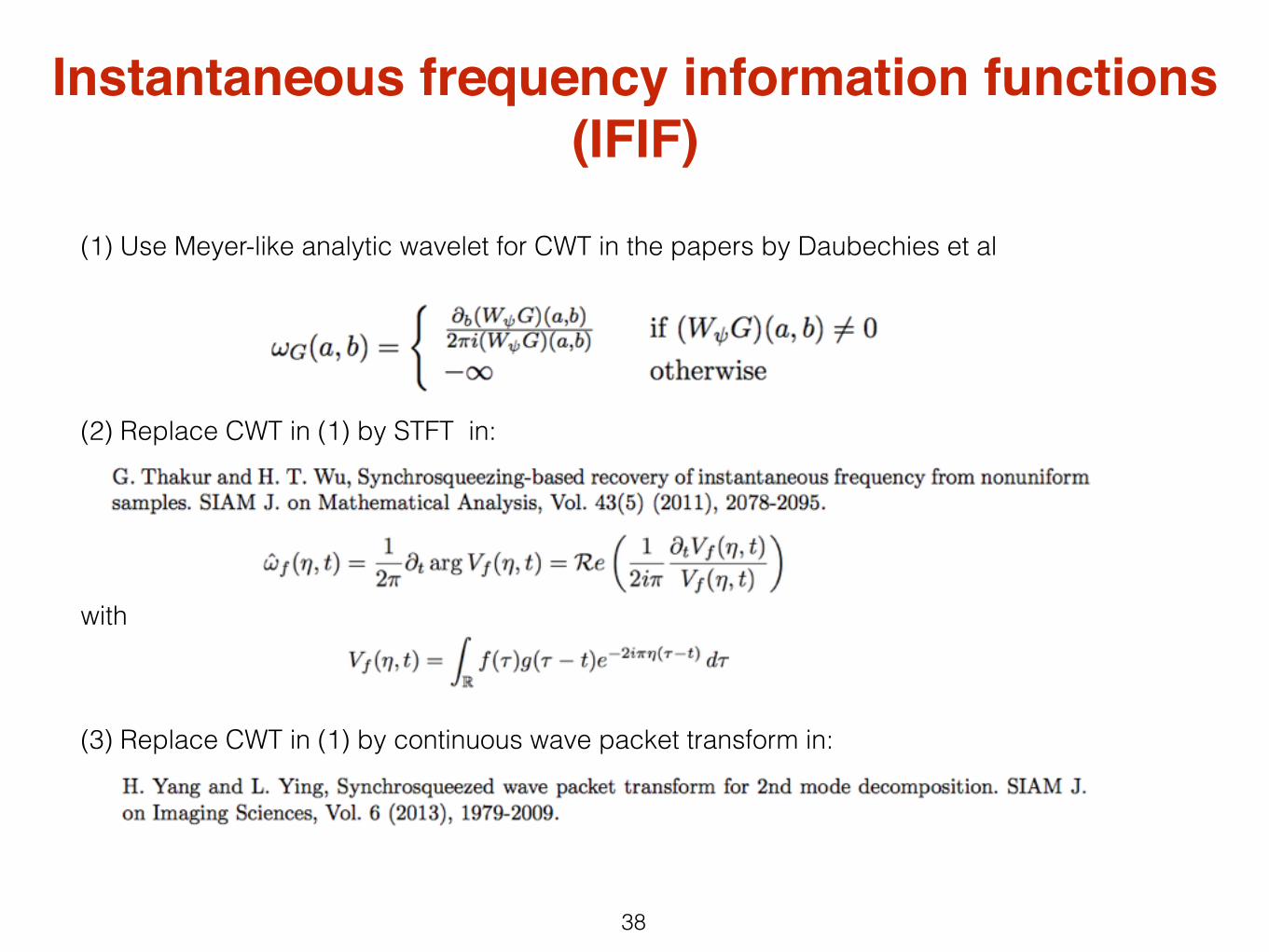
Instantaneous frequency information functions (IFIF)

(1) Use Meyer-like analytic wavelet for CWT in the papers by Daubechies et al

(2) Replace CWT in (1) by STFT in:

with

(3) Replace CWT in (1) by continuous wave packet transform in:

38

Synchrosqueezing transforms (SST)

The IF’s of possible sub-signals are estimated from one of the two point-sets

by curve fitting or other “interpolation” schemes, depending on CWT or STFT are to being used.

Note: t=b, and the other two symbols are used to denote the same frequency variable.

39

or

or

SST recovery of sub-signals from IF’s

Note: Since the IF’s are used as the limits of integration, they could be very poor estimates (as a result of their dependence on “curve fitting”), so that the results of signal decomposition may not be satisfactory.

Also, the big challenge by applying SST is to guess correctly the number (“M” in the AHM) of IF curves to be fitted, or equivalently the number of sub-signals to be recovered.

40

Outline of SST for IF estimation and recovery of sub-signals

• The three steps in instantaneous frequency (IF) estimation are:

1. Computation of an IF information function (IFIF).

2. For each fixed time instant, threshold the IFIF, and apply SST integral formula at this fixed time instant to extract the desired well-separated IF data.

3. Apply curve fitting or a desirable “interpolation” scheme to compute the estimated (continuous-time) IF functions.

• Using the estimated IF functions, apply certain integral formula to recover the sub-signals.

41

Some limitations of the SST approach for blind-source signal decomposition

• Number of IF functions cannot be determined in general.

• As a result, not all sub-signals can be recovered in practice.

• It is difficult, if at all feasible to separate two sub-signals with the same IF but different phases (say, by some additive constant).

• Sub-signal recovery integral formula suffer from inaccurate IF estimation and phase distortion.

42

Example 1: Extraction of frequencies from two-frequency signals

Source: Hau-tieng Wu, Patrick Flandrin and Ingrid Daubechies (Adv. Adapt. Data Anal., 2011)

See Slides # 31, 32 on the unacceptable EMD IF extraction result by using Hilbert transform of the two IMF’s

43

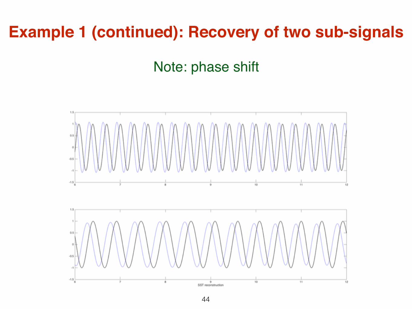
Example 1 (continued): Recovery of two sub-signals

Note: phase shift

44

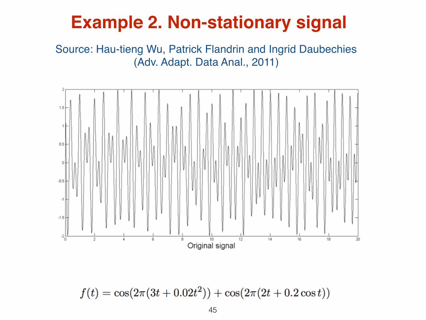
Example 2. Non-stationary signalSource: Hau-tieng Wu, Patrick Flandrin and Ingrid Daubechies

(Adv. Adapt. Data Anal., 2011)

45

SST extracts the IF information function for

curve fitting (below) and

two sub-signals (in black, on right) Note: phase shift

46

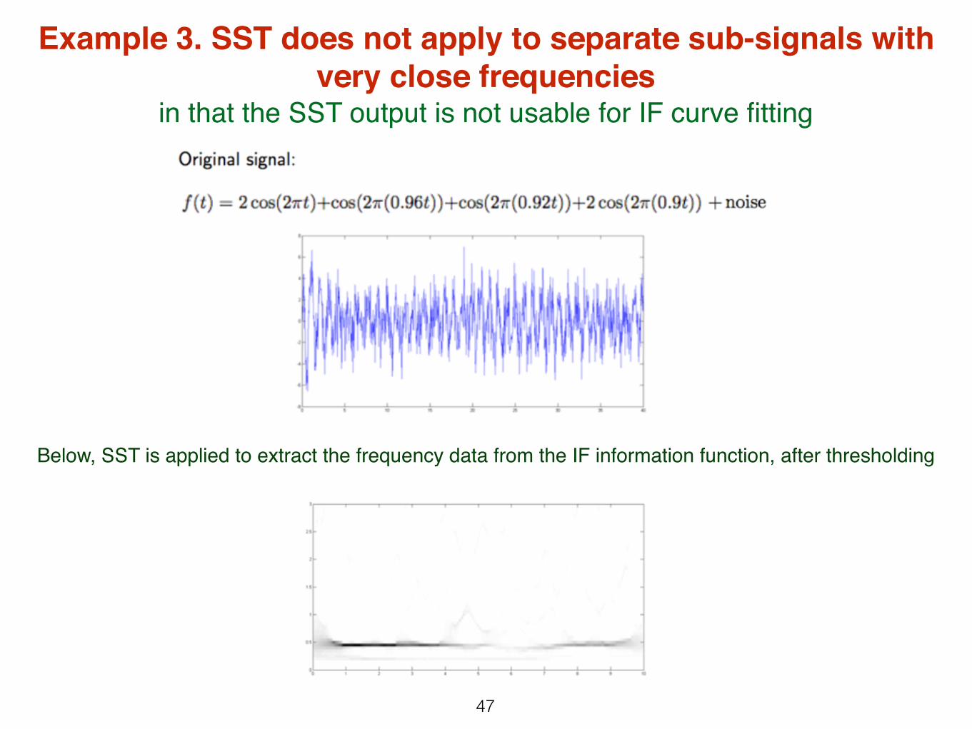
Example 3. SST does not apply to separate sub-signals with very close frequencies

in that the SST output is not usable for IF curve fitting

47

Below, SST is applied to extract the frequency data from the IF information function, after thresholding

5. Direct time-frequency approach:

Phase-preserving sub-signal separation operation (or operators), (PSSO)

using the AHM, under certain mild specifications

48

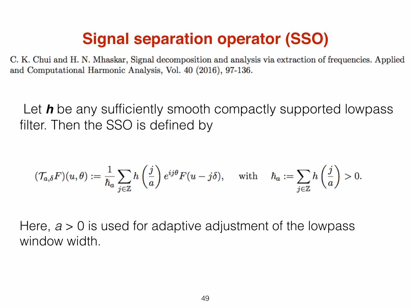
Signal separation operator (SSO)

Let h be any sufficiently smooth compactly supported lowpass filter. Then the SSO is defined by

Here, a > 0 is used for adaptive adjustment of the lowpass window width.

49

Computation flow diagram of PSSO

50

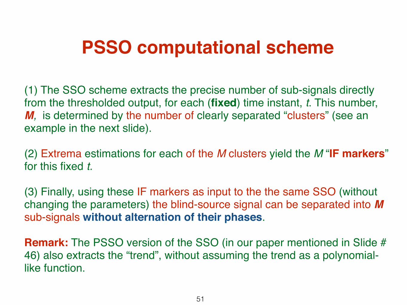
PSSO computational scheme

(1) The SSO scheme extracts the precise number of sub-signals directly from the thresholded output, for each (fixed) time instant, t. This number, M, is determined by the number of clearly separated “clusters” (see an example in the next slide).

(2) Extrema estimations for each of the M clusters yield the M “IF markers” for this fixed t.

(3) Finally, using these IF markers as input to the the same SSO (without changing the parameters) the blind-source signal can be separated into M sub-signals without alternation of their phases.

Remark: The PSSO version of the SSO (in our paper mentioned in Slide # 46) also extracts the “trend”, without assuming the trend as a polynomial-like function.

51

Illustration of SSO output clusters for each fixed time instance t

Source of example: Hau-tieng Wu, Patrick Flandrin, and Ingrid Daubechies (Adv. Adapt. Data Anal., 2011)

52

Illustration of SSO output clusters after thresholding

53

Returning to Example 2 (See Slides # 42, 43)

SSO extracts M = 2 components and yields 2 IF’s (in black, below),

from the IF pointers and

2 sub-signals (in black, on right)

54

Returning to Example 3 (see Slide #44)

where the original (input) function f (t ) (minus the noise) is unknown

55

PSSO discovers 4 IF pointers and extracts 4 IF’s

56

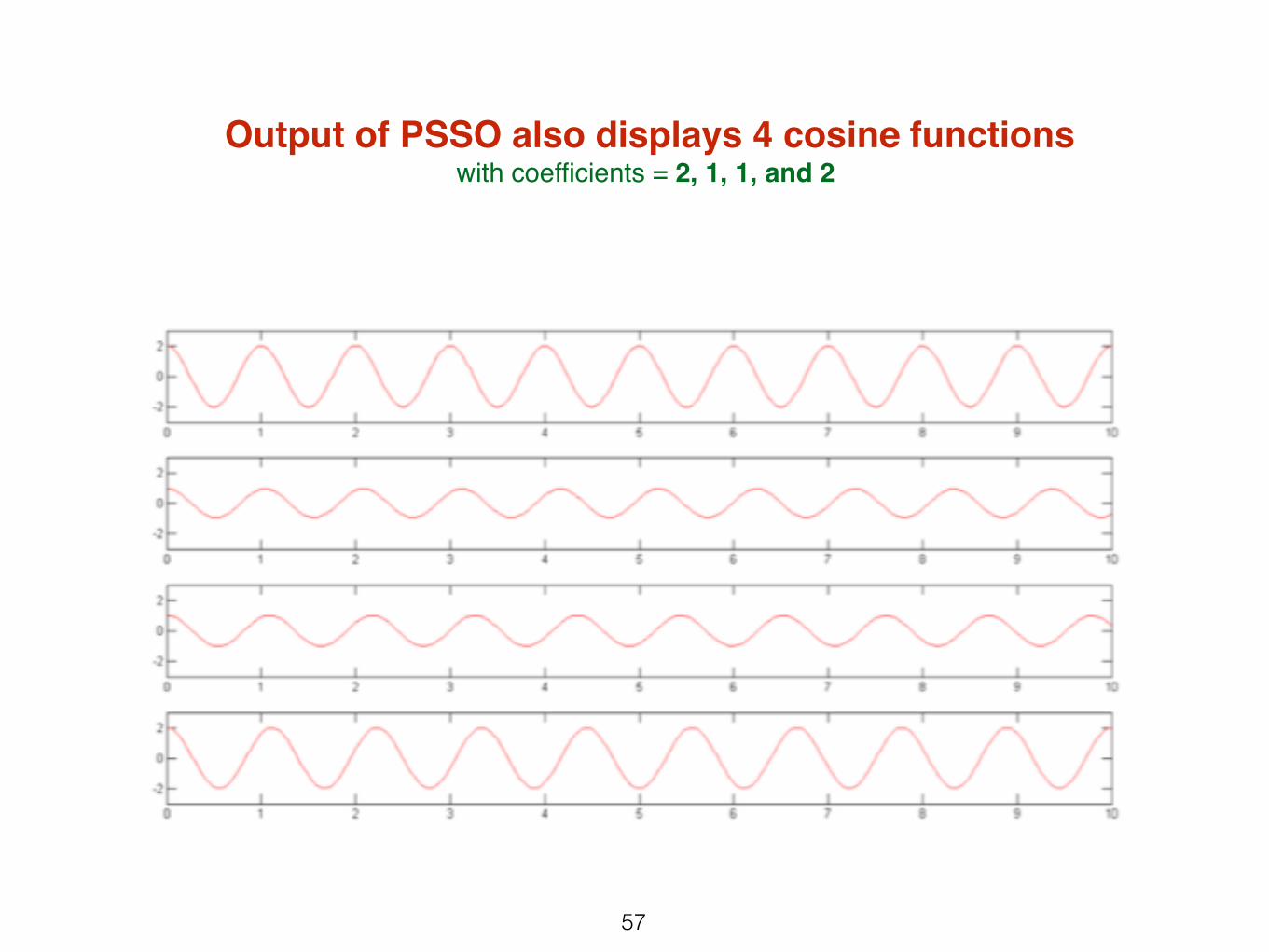
Output of PSSO also displays 4 cosine functions with coefficients = 2, 1, 1, and 2

57

6. Remarks and discussions

58

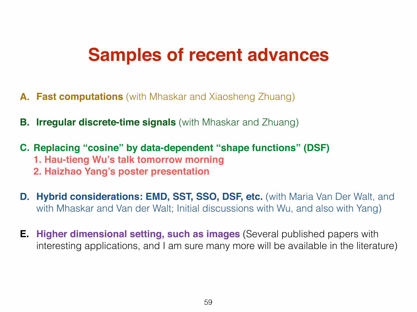
Samples of recent advances A. Fast computations (with Mhaskar and Xiaosheng Zhuang)

B. Irregular discrete-time signals (with Mhaskar and Zhuang)

C. Replacing “cosine” by data-dependent “shape functions” (DSF) 1. Hau-tieng Wu’s talk tomorrow morning 2. Haizhao Yang’s poster presentation

D. Hybrid considerations: EMD, SST, SSO, DSF, etc. (with Maria Van Der Walt, and with Mhaskar and Van der Walt; Initial discussions with Wu, and also with Yang)

E. Higher dimensional setting, such as images (Several published papers with interesting applications, and I am sure many more will be available in the literature)

59

Thank you for

your attention

60